power consumption of reed-solomon decoder...

EXAMENSARBETE

2002:289 CIV

MASTER OF SCIENCE PROGRAMME

Department of Computer Science and Electrical EngineeringDivision of Computer Engineering

2002:289 CIV • ISSN: 1402 - 1617 • ISRN: LTU - EX - - 02/289 - - SE

Power Consumption ofReed-Solomon Decoder Algorithms

STEFAN RYSTEDT

Power consumption of Reed-Solomon

decoder algorithms

Master’s Thesis in Computer Science

Stefan Rystedt

May 2001

Examiner:

Per Lindgren

Division of Computer Engineering

Department of Computer Science and

Electrical Engineering

Luleå University of Technology

Supervisor:

Martin Malmström

UN/D

Ericsson Microwave Systems AB

Mölndal

Abstract

The Core Unit ASIC Technology & System on Silicon at Ericsson Micro Wave Systems has a

project on STM-1 / SDH communication over a microwave link called Mini Link. They want to

have a power effective Reed-Solomon encoder to correct bit errors. In this master’s thesis three

different algorithms for Reed-Solomon codes are implemented in hardware using VHDL and

then compared by power consumption. The Reed-Solomon code implemented is an RS(255,239)

that handles errors but not erasures.

The different algorithms used are Berlekamp-Massey, Gröbner basis by Fitzpatrick and Welch-

Berlekamp. They are implemented in VHDL and first compared by the size after being

synthesized, then compared by power dissipation estimated for non, four and eight errors per

block with Watt Watcher from Sequence. The Berlekamp-Masey had the lowest power

dissipation for all error rates and the smallest size. However, no real winner could be selected

among the algorithms since the differences in size and power dissipation where so small.

Acknowledgements

I would like to thank my fiancée for being supportive when nothing seemed to go my way. I

also want to thank the people at Ericsson Microwave Systems AB in Mölndal where this

master’s thesis is written. Especially Anders Persson for the Unix support. Martin Uddeborg,

Magnus Carlsson, Carl Gustafsson and Joachim Strömbergson for their pranks and incredibly

intelligent conversations that kept me alert at all times, and my supervisor Martin Malmström for

all support and material.

I also would like to thank Paul Rowley from Sequence for helping me with Watt Watcher,

Patrick Fitzpatrick for explaining details in his algorithm. Last, I would like to thank my

supervisor at Luleå University of Technology (LTU) for his quick responses.

Stefan Rystedt

Table of contents

1 Introduction 1

2 Power Dissipation 3

3 Galois field 5

4 Reed-Solomon code 74.1 Encoding 7

4.2 Decoding Algorithms 8

4.2.1 Berlekamp-Massey & Fitzpatrick 8

4.2.2 Welch-Berlekamp 11

5 Implementation 155.1 Parallelism 16

5.2 Galois field operations 16

5.2.1 Multiplication 17

5.2.2 Inversion 18

5.2.3 Division 18

5.3 Berlekamp-Massey 18

5.3.1 Syndrome block 18

5.3.2 Key equation block 18

5.3.3 Error Locator and Error Corrector blocks 19

5.4 Fitzpatrick 19

5.5 Welch-Berlekamp 19

6 Verification 21

7 Comparisons 237.1 Size 23

7.2 Power estimations 24

8 Conclusions 27

9 Future works 29

10 Glossary 31

11 References 33

Appendix A Berlekamp-Massey key equation I

Appendix B Fitzpatrick key equation III

Appendix C Welch-Berlekamp key equation V

1

1 Introduction

The Core Unit ASIC Technology & System on Silicon at Ericsson Micro Wave Systems

has a project on STM-1 / SDH1 communication over Mini Link

2. In all communications

with digital data, it is likely to have bit errors in the transmission. This is also the case in

the communication over the Mini Link. Several error-control codings (ECCs) can be used

to find and correct errors in a digital data stream. The different ECCs have different

advantages; some are good at random errors and others at burst errors. One ECC that is

good at correcting burst errors is Reed-Solomon. It will be used together with the Viterbi

coding (which are better at random errors) to find and correct the errors in the data stream

transmitted over the Mini Link.

Ericsson Micro Wave Systems already has an implementation of the Viterbi encoder/

decoder that they can use and they have bought a Reed-Solomon encoder/decoder as an IP

(Intellectual Property). However, they would like to have an own implementation of the

Reed-Solomon encoder/decoder that is fit for their special needs. What they want is a

decoder that can correct up to eight symbol errors of 255 symbols where the symbol size is

eight bits. The ASIC with the implemented Reed-Solomon code will be in the Mini Link

together with several other ASICs and they want to keep the temperature down. The power

consumption is getting a larger and larger problem when putting more and more in the

same chip, therefore it is more important to have low power implementation in mind when

building hardware.

There are several different algorithms for the Reed-Solomon coding. In this master’s

thesis, three of them have been implemented in hardware. They are compared by power

dissipation to see if there are any big advantages to choose one over the others.

1 SDH is a transmission standard for digital telecommunication. STM-1 gives that the transfer rate are

155.52Mb/s2 Mini Link is an Ericsson product to wireless transfer digital data from one point to another with

microwaves.

3

2 Power Dissipation

The sources of power dissipation can be divided into two categories, dynamic and static.

The dynamic power dissipation consists of the power consumed to switch the signals. The

static is the power consumed to hold the signals.

According to Demmer [1], about 99% of the total power dissipation is dynamic. This

means that unless there is almost no activity in the design, the static power dissipation can

be discarded. However, this might not be true for future technologies. With smaller

geometry’s the leakage in transistors increase and hence the static power dissipation.

The dynamic power dissipation can be divided into a few categories. First, there is the

clock tree that will consume power every time the clock signal switches. To reduce the

power dissipation for the clock tree, the supply voltage can be minimized. A lower supply

voltage will result in slower gates so that the maximum clock frequency will become

lower. Another approach is to make the design parallel and in that way lower the clock

frequency needed. Clock gating could also be used to stop the clock for the part of the

design that does not do any work at the present. Since both the clock frequency and the

supply voltage were already decided in the specification for the Reed-Solomon, and the

clock gating is quite complex, no power optimization was done for the clock tree.

The second block is the registers. They also consume power as the clock switches,

regardless of the input signals. However, they consume more power if the input switches.

To minimize the power dissipation from the registers the number of registers should be

minimized as much as possible. The switching on the input should also be kept as low as

possible.

Last, there is the logic between the registers. This logic only consumes power when the

signal in the logic switches. The signals that switch often should travel through as little

logic as possible and let the signals that more seldom switch take the longer way. The size

of the logic should also be kept at a minimum. One way to do that is to reduce the number

of complex operations by transforming mathematical expressions like X2+aX+b to

X(X+a)+b .

5

3 Galois field

Reed-Solomon codes are based on Galois fields, see Waltrich [2], also known as finite

fields. The Galois field consist of a finite number of elements and has the property that

arithmetic operations (+,- ,* , / ) on field elements always have a result in the field. The

notation GF(q) where q=pm

is used to denote a Galois field. If p equals two then m is

equal to the number of bits in each symbol. In the rest of this master’s thesis, p is assumed

to be two, since the binary representation is well suited for hardware implementation. The

elements in the field are usually denoted a0,a1

,…,aq - 1. To construct a Galois field, the

degree of the field (i.e. the value of q ) and a primitive polynomial most be decided. For

GF(256) there are 16 such polynomials. To calculate a you can use the formula

a i=2

imod(P(2)) (4.1)

where P(x) is the primitive polynomial. Note that in a Galois field aq - 1 always equals

one. The primitive polynomials can be found by calculating aq - 1 for all different poly-

nomials with degree m . The polynomials that gives aq - 1=1 are primitive polynomials.

To calculate a i + 1 from the m bits symbol a i

, shift the bits of a i left one step and check if

the bit m+1 is set. If it is, do a xor between the result of the left shift of a i and the

primitive polynomial P(2) .

In table 1, The field for GF(16) with the primitive polynomial P(x)=x4+x+1Ú

x4=x+1 is calculated. GF(16) has four bits per symbol, a0

,a1,a2

,a3 represents the

four bits. a0 is the LSB (Least Significant Bit) and a3

is the MSB (Most Significant Bit)

and as shown in table 1 the rest of the symbols is built upon combining these.

6

a0=1

a1=a1

a2=a2

a3=a3

a4=a+1

a5=a2

+aa6

=a3+a2

a7=a4

+a3=(a+1)+(a3

)=a3+a+1

a8=a4

+a2+a=(a+1)+(a2

+a)=a2+1

a9=a3

+aa1 0

=a4+a2

=(a+1)+(a2)=a2

+a+1

a1 1=a3

+a2+a

a1 2=a4

+a3+a2

=(a+1)+(a3+a2

)=a3+a2

+a+1

a1 3=a4

+a3+a2

+a=(a+1)+(a3+a2

+a)=a3+a2

+1

a1 4=a4

+a3+a=(a+1)+(a3

+a)=a3+1

a1 5=a4

+a=(a+1)+(a)=1

Table 1 GF(16) with the primitive polynomial P(x)=x4+x+1Úx

4=x+1

Adding and subtracting in Galois field is exactly the same thing namely a xor function, e.g.

with the Galois field in table 1 a5+a8

=a5-a8

=(a2+a)+(a2

+1)=a+1=a4. Multipli-

cation is simply an addition of the powers modulus the number of elements in the field

minus one.

aa³a b=a ( a + b ) m o d ( q - 1 )

(4.2)

Division is subtraction of the powers modulus the number of elements minus one.

( )1mod)( --= qba

b

a

aaa

(4.3)

Inversion is done by taking the exponent modulus the number of elements minus one.

a - a=a - a m o d ( q - 1 )

(4.4)

7

4 Reed-Solomon code

The Reed-Solomon code is an error correcting code with which bit errors in transmitted

words can be found and corrected. It has become an important coding technique when

transmitting digital data due to its large burst error correction capability with minimal

added data bits. It is a block code, which means that the data is sent in blocks of symbols

where the number of symbols per block is in relation to the number of bits in each symbol.

The formula is

n=2b-1 (5.1)

where n is the number of symbols per block and b the number of bits per symbol. There

are d data symbols, which is the actual data to send, and p parity symbols, which is

redundant data built on the data symbols. Reed-Solomon codes are often denoted as

RS(n,d) so in an RS(15,11) there are 15 symbols per block, 11 data symbols and 15-

11=4 parity symbols. As mentioned earlier the number of bits per symbol decides the

Galois field, so for the RS(15,11) a GF(16) is used. To correct an error in one symbol

two parity symbols are needed, so the total number of errors ( t ) that can be corrected are

2

pt = . (5.2)

In the RS(15,11) code, up to two symbol errors can be corrected since 2

4=t . If some

symbols that are received are highly unreliable, they can be marked as erased. To correct

an erased symbol only one parity symbol is needed since the location of the broken

symbols is known. Therefore, the total number of errors ( t ) and erasures (s) that can be

corrected are

p=2t+s . (5.3)

If 2t+s>p one thing of two can happen, either the decoder will detect that it can not

recover the code word and flag this, or it will miss-decode and recover an incorrect word.

4.1 Encoding

Most Reed-Solomon codes are systematic codes; this means that the encoder just adds the

parity symbols without modifying the data symbols.

To generate a systematic code a generator polynomial is needed. All valid code words are

exactly divisible by this polynomial. The general formula to calculate the polynomial is.

( ) ( )Ô-

=

++=1

0

p

i

ijxxG a (5.4)

where j is an integer and p is the number of parity symbols.

One easy way to calculate the parity symbols in hardware is to use a p stage feedback shift

register, see figure 1.

8

Figure 1. Reed-Solomon decoder using a p stage feedback shift register.

The constants b1 to bP are calculated from the coefficients of the generator polynomial,

G(x)=gpxp+gp - 1x

p - 1+…+g1x+g0 by the formula.

0g

gb i

i = (5.5)

The data symbols are fed one by one to the encoder. The data is put on the output through

multiplexer B and to the registers through multiplexer A. So the data symbols are

immediate put on the output without any altering. When the decoder has received all data

symbols. Multiplexer A sends zeros to the registers and multiplexer B sends the, by the

registers, calculated parity symbols. When p parity symbols ha been sent all registers are

cleared and the decoder is ready to decode next block of data.

4.2 Decoding Algorithms

There are several different algorithms to decode reed-Solomon codes. In this master’s

thesis three of them are implemented and then compared regarding to the power

consumption. The three different algorithms are Berlekamp-Massey Johannesson et al [3],

Gröbner basis by Fitzpatrick [4] and Welch-Berlekamp Chambers et al [5]. The decoder

for the Mini Link only has to handle errors and not erasures. Therefore, the part of the

algorithms that handles erasures has been left out.

4.2.1 Berlekamp-Massey & Fitzpatrick

The Berlekamp-Massey algorithm was chosen because it is a well-known algorithm and

has often been used in hardware implementations. The Fitzpatrick algorithm has the same

architecture as the Berlekamp-Massey, see figure 2, only the key equation to calculate the

Error Locator Polynomial differs. It was chosen since it is claimed to be more efficient to

implement in hardware than the Berlekamp-Massey key equation.

Figure 2 The design of Berlekamp-Massey or Fitzpatricks algorithm.

0

Encoded data

In d

ata

1b2-Pb1-PbPb 2b

GF multiplication

GF addition

A

B

Syndrom

Error LocationPolynomial

Berlekamp-Masey

orFitzpatric key

equation

ErrorLocation

Chien search

ErrorMagnitude

Forney’salgorith

S(x)

R(x)

ELP(x) ix

ii xe

9

First, a Syndrome is calculated, this is used to calculate an error polynomial. The degree of

the error polynomial is the same as the number of errors. From the roots of the error

polynomial, the error locations can be calculated. Last, the Syndrome, the error locations

and the error polynomial are used to calculate the error magnitude.

When using the feed back shift register decoder, the formula to calculate the generator

polynomial (eq 5.4) has to be modified. The new formula is

( ) ( )Ô=

-+=p

i

ixxG1

a . (5.6)

Say that the sent word is V(x) and the received code word is R(x) then

R(x)=V(x)+E(x) , (5.7)

The error polynomial E(x)=Se ixi, where e i is the Magnitude of the error and x

i is the

position of the error.

Taking the Discreet Fourier transform (DFT) gives

R(x)=V(x)+E(x) (5.8)

where R and V are the Fourier transform of R and V respectively.

It can be proved that

V j=0, j=d,d+1,…,n-1 (5.9)

and hence from (eq 5.8)

R j=E j j=d,d+1,…,n-1 (5.10)

i.e. n-d consecutive components of the DFT of the error patterns can be computed at the

receiver. If the remaining d components could be found, the inverse Fourier Transform

(IDFT) could be used to obtain the error polynomial E(x).

If there are at most t errors the cyclic complexity of E(x) is at most t . This means that

there is a polynomial L(x) of degree at most t that can generate E(x) from t consecutive

components of E(x) by the formula

( ) 1,,1,0,1

-=L= ä=

=+ nj

tl

l

2nlmodjlj EE (5.11)

When the n-d components of E(x) are calculated, an Error Locator Polynomial L(x) can

be found with L0=1 that can generate E(x) with the equation (5.11), by solving a system

of t linear equations

10

öööööö

÷

õ

ææææææ

ç

å

=

öööööö

÷

õ

ææææææ

ç

å

L

LLL

öööööö

÷

õ

ææææææ

ç

å

+

+

+

++++

-+-+-+

-+++-+

-+++++

d

3-td

2-td

1-td

td3d2d

tdd

1tdtdd

2td1tdtd

E

E

E

E

EEEE

EEEE

EEEE

EEEE

44

3

4444

4

4

4

1

3

21

1

1

312

21

1

td

ntdt

nt

n

(5.12)

The Error Locator Polynomial has the form

( ) ( )Ô=

+=Lk

1l

ixx la (5.13)

where i l , l=1,2,…,k¢ t is the error locations for the at most t errors.

Since the IDFT of E(x) is quite complex to implement in hardware the Forney algorithm

is used. The Forney algorithm uses the n-d components of E(x) and the Error Locator

Polynomial to calculate E(x) .

4.2.1.1 Syndrome calculation

The calculation of the Syndrome S(x) with degree p-1 is done by calculate the DFT for

Ej, j=d,d+1,…,n-1 where

( )( )( )

( ) öööööö

÷

õ

ææææææ

ç

å

=

öööööö

÷

õ

ææææææ

ç

å

=

öööööö

÷

õ

ææææææ

ç

å

-

-

-

-d

n

n

n

p R

R

R

R

S

S

S

S

a

aaa

444

3

2

1

1

2

1

0

d

3-n

2-n

1-n

E

E

E

E

(5.14)

4.2.1.2 Error Locator Polynomial

From the Syndrome, the Error Locator Polynomial L(x) can be found from the equation

(5.12). The Berlekamp-Masey or the Fitzpatrick key equation is used to solve it. The

Berlekamp-Masey key equation is shown in appendix A and the Fitzpatrick key equation

in appendix B.

4.2.1.3 Error locations

To calculate the error location; the roots of the error polynomial L has to be calculated.

This is done by Chien search. Calculate the result of the error polynomial for every

element in the Galois field and see if it equals zero. If L(a i)=0, i=0,1,…,n-1 then a i

is a root and the location of the error is xi.

If the number of roots does not match the degree of the polynomial, there are more errors

than can be corrected.

11

4.2.1.4 Error Magnitude

When the error locations are known the error magnitude can be calculated using the

Forney algorithm.

Calculate the modified error locator polynomial W.

W (x)=S(x)L(x )mod(xp) . (5.15)

Calculate L’ (x) .

The error magnitude at the error location xi is

( )( )i

i

ieaa

L¡W

= . (5.16)

Last, subtract the error polynomial E(x) with the received word R(X) to get the sent word

V(x) .

4.2.2 Welch-Berlekamp

Figure 3 The design of the Welch-Berlekamp algorithm

The Welch-Berlekamp algorithm has a different architecture than the two above, see figure

3.

First it has a recoding stage where new parity symbols are calculated, then there is a

calculation of a key-equation and last a Chine search to find the roots and from them the

error magnitude.

First, some definitions have to be made.

Let U be the set {0,1…n-1} and V any subset of U then define

( ) ÔÍ

-=Vi

ixxVf )(; a . (5.17)

If V is the empty set then f (V;x)=1 .

We also define

f ’ (V;x)=f(V-{i};x) . (5.18)

Here V-{i} denotes deletion of the member {i} from the set V .

Recoder Key

ErrorLocation

Chien search

ErrorMagnitudeY(x)

R(x)

Q(x) ix

ii xe

P(x)

12

Let D be the data symbols set {0,1,…,d-1} and P be the parity symbols set P=U-

D={d,d+1,…,n-1} .

4.2.2.1 Recoding

Say that the sent word is V(x) and the received code word is R(x), recode the data

symbols D in R(X) , i.e. calculate new parity symbols, to get a new code word RC(X).

Then calculate Y(x) by subtracting the parity symbols from the recoded word with the

parity symbols from the received word and multiply the result with a constant.

y i=(rc i + d-r i + d )f ’ (P;a i + d) , i=0,1,…,p-1. (5.19)

Y(x) is then used when solving the key equation below. Notice that if there are no errors

the parity symbols for the recoded word and the received word are the same and rc i + d-

r i + d=0 hence Y(X) will be the zero polynomial.

4.2.2.2 Key equation

The key equation to solve is

y iQ(a i + d)=P(a i + d

) , i=0,1,…,p-1. (5.20)

Where the error location can be calculated from Q(x) and the error magnitude from P(x)

and the derivate of Q(x) . The key equation can be found in appendix C.

4.2.2.3 Calculating the error location.

The roots of the polynomial Q(x) have to be found. This is done with Chien search as in

the two algorithms above.

If a i is a root to Q(x) then the error location is x

i.

If the number of roots does not match the degree of the polynomial, there are more errors

than can be corrected.

13

4.2.2.4 Calculating the error magnitude.

The error magnitude e i at error location xi are calculated by the equation

( )( ) ( ) Di

PfQ

Pe

ii

i

i Í¡

= ,;aa

a(5.21)

There are also equations to calculate the error magnitude for the parity symbols, but they

are left out in this master’s thesis.

15

5 Implementation

The Reed-Solomon code that should be implemented in hardware is an RS(255,239)

code over the GF(256) , which means that the symbol length is 8 bits. The primitive

polynomial for the GF(256) is x8+x

4+x

3+x

2+1 . The decoder should not handle

erasures only errors. It should be able to fetch and process a new symbol every clock cycle.

Since the minimum data rate it should be able to handle is 155.52 Mbit, the clock

frequency has to be at least

khz8.20

8*255

239

10*52.155 6

º

The Hardware implementation was made in Renoir where the design blocks were created

and connected. All the blocks were then implemented as VHDL code using Emacs. All

three implementations have the same interface of the decoder see figure 4.

Figure 4 The symbol for the decoders.

When DV_RS_DEC is set the symbol on the D_RS_DEC is read and the internal number

of symbols per block count is increased by one. When the LB_RS_DEC and DV_RS_DEC

are both set the symbol on D_RS_DEC is considered the last symbol for this block. If the

number of symbols for this block is not equal to 255, the block is thrown away without any

reports. If the number of symbols equals 255, the block is processed to find the error

locations and magnitudes if any.

When DV_RS_DEC_O is set the decoded symbol on D_RS_DEC_O is valid. If both

DV_RS_DEC and LB_RS_DEC are set, the last symbol in this block is valid on the

output.

If the ERR_RS_DEC_O is set with the LB_RS_DEC_O there are too many errors in this

block to be corrected.

16

All algorithms take more than 2³255=510 clock cycles but less than 3³255=765 clock

cycles to decode a symbol. Since all algorithms only calculates the error magnitude of the

erroneous symbol all the data symbols received in the decoder has to be stored in the

decoder. The block length is 255 symbols that means that 3 blocks of data has to be stored,

but it is only the data symbols that are of interest. Therefore only 3³239=717 symbols

have to be stored. This could be done with simple registers but since registers tends to

consume much power, a dual port synchronous SRAM is used instead.

5.1 Parallelism

All the algorithms are described in a serial style, which is okay, if implemented in

software. In hardware on the other hand, parallelism is desirable. Therefore, an analysis of

the algorithm has to be done to see what can and should be made in parallel. Parallelism

increases the speed at which the calculation can be performed, i.e. the number of clock

cycles it takes. It can also increase the size of the implementation. Since the decoder

should be able to receive one symbol per clock cycle, no stages can take more than 255-

clock cycles to complete. Hence, some parallelism has to be implemented.

The calculation of type y=F(a i) is never done in parallel. Taking the power of a Galois

field element is very complex, which has to be done if the degree of F is larger than 1.

Therefore the fact that ax3+bx

2+cx=d is equal to x(x(xa+b)+c)+d is used. This

calculation is then easily done in four steps with only one single Galois field multiplication

and addition.

1. y=xa

2. y=x(y+b)

3. y=x(y+c)

4. y=y+d

The calculation of type Y(x)=F(x)³a i can be described as

y1=f1³a i

y 2=f2³a i

4

yd=fd³a i

which is best implemented in parallel with 16 Galois field multiplications. For the different

key equations there are many different calculations made in parallel.

5.2 Galois field operations

The more complex operations in the Galois field: inversion, multiplication and division are

implemented as functions in a VHDL package.

17

5.2.1 Multiplication

As mentioned before, multiplication in Galois Field is only addition of the powers. The

problem is that in hardware there is only the binary representation of the symbols. Since

the hardware can not say directly what the symbol representation is by looking at the bit

representation. There has to be a look up table with 255 entries to translate the bit

representation to the symbol representation. This would result in very large hardware since

there are many multiplications in the algorithms. What is known is that a0,a1

,…,a7

represents the eight bits. a0 is the LSB and a7

is the MSB and all the rest of the symbols

are made of adding this symbols together. By using that if a³b=c and a=d+e then

(d+e)b=d³b+e³b=c . The multiplication of two symbols can be divided into several

multiplications where one of the multiplicands is one of a0,a1

,…,a7. As example take

a³b , where a and b is element in the GF(256) used for the encoder. Say that a=a3 5, the

bit representation of a3 5 is “10011100” or a7

+a4+a3

+a2 so the multiplication can be

rewritten as a7³b+a4³b+a3³b+a2³b .

To calculate a i³b, i>0 , repeat the following i times; left shift all bits in b one step then if

the ninth bit in b is set take b modulus the primitive polynomial.

The VHLD code for the multiplication is

- The primitive polynomial: x^8+x^4+x^3+x^2+1

constant PRIMITIVE_POLYNOMIAL : std_logic_vector(8 downto 0) := "10001111";

function GF_MULT (A,B : in std_logic_vector (7 downto 0))

return std_logic_vector is

variable I,J : integer; -- Counters

variable TEMP : std_logic_vector (8 downto 0);

variable ANSWER : std_logic_vector (7 downto 0);

begin

if A(0) = '1' then

ANSWER := B;

else

ANSWER := (others => '0');

end if;

GF_MULT : for I in 1 to 7 loop

if A(I) = '1' then

TEMP(8) := '0';

TEMP(7 downto 0) := B;

GF : for j in 1 to I loop

TEMP := TEMP(7 downto 0) & '0';

if TEMP(8) = '1' then

TEMP := TEMP xor PRIMITIVE_POLYNOMIAL;

end loop GF;

ANSWER := TEMP(7 downto 0) xor ANSWER;

end loop GF_MULT;

return ANSWER;

end GF_MULT;

18

5.2.2 Inversion

The inversion is very complex in Galois field to which no easy solution was found.

Therefore the inversion is simply done by a truth table with 255 entries, all optimizations

are then left to the synthesis tools. This result in a much bigger hardware than for the

multiplication, fortunately inversion is quite rare in all the algorithms.

5.2.3 Division

The division is simply done by inverting one of the terms before the multiplication.

This of course results in even larger hardware than the inversion it self, but also division is

rare in the different algorithms.

5.3 Berlekamp-Massey

5.3.1 Syndrome block

The 16 syndrome elements are calculated in parallel as in figure 5. When all symbols in a

block are received the calculation of S(X) is finished and sent to the next block and all the

registers are cleared.

There is the same amount of calculations done regardless of the error rates. Therefore is

the power dissipation for this step not dependent upon the number of errors in the block.

Figure 5 The parallel calculation of the syndrome.

5.3.2 Key equation block

The calculation of the Error Locator Polynomial with the Berlekamp-Massey algorithm,

see appendix A, is divided in two steps that are repeated 16 times. One that calculates)(kD (Appendix A step 3) this takes L clock cycles. The other calculates the rest in just one

clock cycle.

1a0S

2a 1S

16a 15S

( )xS

ReceivedSymbol

GF multiplication

GF addition

19

The number of times D ( k ) not equal to zero is dependent upon the number of errors. Since

there is less calculation done if D ( k ) equals to zero there will be less signals that are

shifting values and hence less power dissipation. Therefore, with low error rates the power

dissipation will be less than with high error rates for this block

5.3.3 Error Locator and Error Corrector blocks

The calculations of type F(a i) , with degree deg, are done by a piped calculation as in

figure 6. In the Error Locator block the calculation of the Modified Polynomial and the

derivate of the Error Locator Polynomial, which is needed by the Error Corrector block,

are made. The calculation in the Error Corrector block is only performed when the Error

Locator has found an error so the power dissipation for this block is dependent upon the

error rates. The Chien search on the Error Locator Polynomial in the Error Corrector block

takes 255 clock cycles to test all possible roots, regardless of the number of errors.

However, the degree of the Error Locator Polynomial is dependent of the number of errors.

With a low degree most of the GF multiplication in the piped calculation will be zero, so

there will be less signal switching and hence less power dissipation.

Figure 6 The piped calculation of F.

5.4 Fitzpatrick

The Syndrome, Chien search and the Forney calculation is done exactly as in the

Berlekamp-Massey algorithm only the key equation to calculate the Error Locator

polynomial differs, See appendix B for the Fitzpatrick algorithm.

The key equation calculation is divided in two steps repeated 16 times. The first calculates

a j (Appendix B step 3) and this takes the degree of bj clock cycles. The other step does

the rest of the calculation and takes one clock cycle. The degree of bj and the number of

times a j are not zero is dependent upon the number of errors. Few errors produce a low

degree of bj and a j is zero more often. Therefore, the power dissipation will be less with

low error rates than with high.

5.5 Welch-Berlekamp

Since f (P;x) , needed by the Error Locator, and f ’ (P;x) , needed by the Recoder, do not

depend upon the data received. They are pre calculated and inserted in the VHDL code as

constants.

The recoding is done exactly as the encoding except for a Galois Field addition between

the old, the new parity symbols, and then a Galois fields multiplication, see equation 5.19.

The power dissipation for the Recoder does not depend on the error rates.

ia

degF 1deg-F

2deg-F 0F

1F

GF multiplication

GF addition

20

The Key equation, see appendix C, is divided in 3 steps repeated 16 times. The first step

calculates d (Appendix C, step 2), it takes the degree of Q(x) clock cycle. The second step

calculates c (Appendix C, step 8), this takes the degree of W(x) clock cycle, and the third

calculates the rest in one clock cycle. If d equals zero there is no need for the second step.

With fewer errors the degree of Q(x) and W(x) is smaller and hence the power

dissipation.

The Error Locator and the Error Corrector block are very similar to those used by the other

two algorithms except that there is no calculation of a modified Error Locator Polynomial.

21

6 Verification

To verify the hardware a software implementation was made in Java. The implementation

in Java was done in a generic way, so that the block length, number of parity symbols and

the Galois field used where variable. This made it possible to verify that the different

stages in the algorithm worked, by using different examples. Operations that seemed

complex to implement in hardware, like Galois field multiplication, was first implemented

in a software style and then as close to hardware as possible.

Constants needed for the algorithm to work were calculated by the software

implementation. It also produces data files that can be used in a Test bench to verify the

correctness of the Hardware implementation. The data files produced can be used either for

the whole design or for some block in the design.

The hardware was verified by a test bench that produce encoded data with errors for the

decoder and then checked that the decoder corrected the blocks that had 8 symbol error or

less. All the implementations passed the test.

23

7 Comparisons

7.1 Size

The VHDL was synthesized to TSMC technology using Ambit from Cadence. It was

synthesized with high effort for area optimization; the clock speed set to 100MHz. The size

of the synthesized design can be seen in figure 7; the size is in number of cells. Since the

size of a cell differs from different vendors and it is the size relative to each other that is

interesting, no axes are given.

Figure 7 The size for the different block and different implementations

As can be seen in figure 7 the size of the implemented algorithms does not differ too much.

Remember that only the Key Equation differs between the Berlekamp-Massey and the

Fitzpatrick algorithm. This means that the other blocks will consume about the same power

in both algorithms. It can also be noted that the size of their key equations is quite small in

comparison to the size of the common blocks. This indicates that the power consumption

will be much higher for the common blocks than for the key equation. This implies that the

algorithm choice for the Key Equation is of secondary importance.

The Syndrome/Recoder is the only block where the power dissipation does not depend

upon the error rates. Since this is the smallest block in the algorithms, the over all power

dissipation probably depends a lot on the error rates of the received symbols.

Size

Syndrom/Recoder Key Equation Error Location Error Magnitude Total with out

memory

Berlekamp-Masye Fitzpatrick Welche-Berlekamp

24

7.2 Power estimations

The power estimation was done with a tool from Sequnce called Watt Watcher. This tool

takes the VHDL code and simulation data and estimates the power consumption. The

estimation would be more accurate if it was done on the synthesized circuit rather then the

VHDL code. This could also be done with Watt Watcher unfortunately there was not time

enough to do that. The Watt Watcher version used was brand new and not so tested since

the design was too complex for the old version. This makes the estimation even more

uncertain. Since the power dissipation should depend on the error rates, the power

dissipation was estimated for none, middle and high error rates. The simulation data is 50

blocks of random generated data with all blocks having the same number of errors. The

errors where inserted at random places with random magnitude. The middle error

estimation contained four errors per block and the high error estimation contained eight

errors per block.

Figure 8 The average power dissipation of the different algorithm at different error rates

The Berlekamp-Masey has the lowest dissipation of the algorithm regardless of the error

rates and Welch-Berlekamp the highest, see figure 8. The Berlekamp-Masey and

Fitzpatrick algorithm has very similar power dissipation as expected from the size

comparison. The differences in power dissipation between low and high error rates are not

as high as expected from the size comparison.

So how is the power dissipation divided among the building blocks in the algorithms?

Total power dissipation

0,000

0,005

0,010

0,015

0,020

0,025

0,030

0,035

0,040

0 errors 4 errors 8 errors

W

Berlekamp-Masey Fitzpatrick Welch-Berlekamp

25

Figure 9 Power dissipation for the different blocks with no errors

Figure 10 Power dissipation for the different blocks with 8 errors

The most of the power dissipation comes from the Syndrome/Recoder block, which was

the only block that did not depend upon the error rates. This would explain why the

differences between none and high error rates are quite small.

In the Syndrome/Recoder 16 Galois field multiplication is done for every symbol in a

block. To process one block of data 16³255=4096 multiplications are performed. The

Syndrome/Recoder might be the smallest block in size, but for every symbol it receives

almost every signal in it switches hence the high power dissipation.

Power dissipation with 8 errors

0,000

0,002

0,004

0,006

0,008

0,010

0,012

0,014

0,016

Syndrome/Recoder Key Equation Error Locator Error Corrector

W


Power dissiaption with no errors

0,000

0,002

0,004

0,006

0,008

0,010

0,012

0,014

0,016

Syndrome/Recoder Key Equation Error Locator Error Corrector

W


27

8 Conclusions

The first block in all the designs dissipates more than half of the total power with no errors.

It is the block with the highest power dissipation even with high error rates. Even if the

estimation is uncertain, it can be seen that a large portion of the power dissipation comes

from the first block. This means that the power optimization should be concentrated on this

block, by finding better ways to calculate the Syndrome or some other way to do the

recoding.

The Key Equation and Error Locator blocks do very little work when there are no errors.

The average power dissipation for these two blocks is therefore approximately the same as

the power consumption due to clock switching in registers. By shutting down the clock for

these two blocks when no work is done, they would consume almost no power at all. The

gain would be greatest for the Welch-Berlekamp since its key equation consumes much

more power than the other two designs.

The Berlekamp-Masey algorithm had the lowest power dissipation for all error rates and

the smallest size. The differences between the Fitzpatrick algorithm and Berlekamp-Masey

where so small that the Fitzpatrick algorithm as well can be chosen. The Welch-Berlekamp

had a little bigger power dissipation than the other two. Mainly because there are more

registers in the key equation and that the recoding is a little more complex than the

syndrome calculation. By finding a more power effective recoding algorithm and using

clock gating it might be more power effective then the other two.

The conclusion is that none of the algorithm has any big advantage over the others when it

comes to power dissipation. The power dissipation is to close and the uncertainty to high.

29

9 Future works

More time could be spent on the power optimisation for the different algorithms. As

mentioned earlier clock gating can be a way to reduce power dissipation. Unfortunately, it

was not possible to use clock gating in this work, but it would be interesting to see how

much gain it would have been when using this.

Today there are power optimisation programs on the market that, by looking at the VHDL

code, give suggestions how to change the code to reduce the power dissipation. It would be

interesting to look at such programs and test them to see how much they can reduce.

The power estimation was now done on the VHDL code. By doing it on the synthesised

circuit, the estimation should be much more accurate.

31

10 Glossary

ASIC Application Specific Integrated Circuit.

DFT Discrete Fourier Transform

GTL Gate Transfer Level.

IDFT Inverse Discrete Fourier Transform

IP Intellectual Property.

LSB Least Significant Bit.

MSB Most Significant Bit.

RTL Register Transfer Level.

SDH Synchronous Digital Hierarchy.

SRAM Synchronous Random Access Memory.

STM-1 Synchronous Transport Module-1.

VHDL Very high speed integrated circuit Hardware Description Language.

33

11 References

[1] Demmer, Christian. Study in Optimization of Low Power ASIC Design on RT-Level,

Ericsson Gothenburg, April 1999.

[2] Waltrich, Joe. Understanding Reed-Solomon Error Correction. Multimedia Systems

Design. December 1998 volume 2, number 12

[3] Johannesson, Rolf & Zigangirov, Kamil Sh. Fundamentals of Convolutional Codes. In

appendix A Reed-Solomon codes. Dec 1996

[4] Fitzpatrick, Patrick. Errors-and-Erasures Decoding of BCH Codes. Dept of

Mathematics, College Cork University, Ireland January 1998.

[5] W. G. Chambers & Zien, Nader F. On the Welch-Berlekamp scheme for decoding

Reed-Solomon codes: a review. Agust 2, 1997

I

Appendix A Berlekamp-Massey key equation

The variables k and L are integers, ( )kD is an element in the Galois field.

( )kL and ( )xT

is polynomial in the Galois field.

1. Initialize the variables ( ) 1,0,0 0 =L== Lk and ( ) xxT = .

2. Set 1+= kk .

3. Compute ( )kD as follows

( ) ( )ä=

---

- L=DL

i

ik

k

k

k ss1

1

1

1 .

4. If( ) 0=D k

, then goto step 8.

5. Modify the polynomial( ) ( ) ( ) ( )xTkkk D-L=L -1

.

6. If kL ²2 , then goto step 8.

7. Set LkL -= and ( )( )

( )k

k

xTDL

=-1

.

8. Set ( ) ( )xxTxT =

9. If pk < goto step 3, where p is the number of parity symbols.

10. The error polynomial L is ( )pL .

III

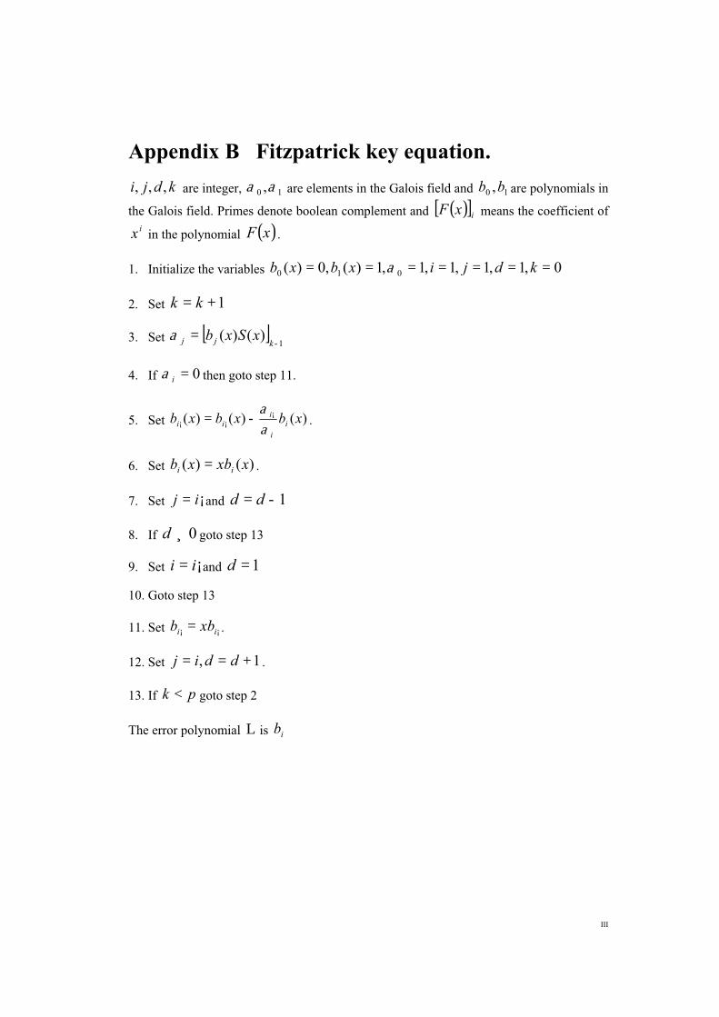
Appendix B Fitzpatrick key equation.

kdji ,,, are integer, 10 ,aa are elements in the Galois field and 10 ,bb are polynomials in

the Galois field. Primes denote boolean complement and ( )[ ]ixF means the coefficient of

ix in the polynomial ( )xF .

1. Initialize the variables 0,1,1,1,1,1)(,0)( 010 ======= kdjixbxb a

2. Set 1+= kk

3. Set [ ]1

)()(-

=kjj xSxba

4. If 0=ia then goto step 11.

5. Set )()()( xbxbxb i

i

iii a

a ¡¡¡ -= .

6. Set )()( xxbxb ii = .

7. Set ij ¡= and 1-= dd

8. If 0¸d goto step 13

9. Set ii ¡= and 1=d

10. Goto step 13

11. Set ii xbb ¡¡ = .

12. Set 1, +== ddij .

13. If pk < goto step 2

The error polynomial L is ib

V

Appendix C Welch-Berlekamp key equation

ji, are integer, d, c are elements in the Galois field and W(x), V(X), P(X), Q(X) are

polynomials in the Galois field.

1. Initialize ( ) ( ) ( ) ( ) 1,0,1,0,0,1 0000 ====== xQxPxVxWji .

2. Calculate ( ) ( )1

1

1

11

-+-

-+-- += di

i

di

ii PQyd aa .

3. If 0¸d then goto step 8.

4. Set ( ) ( ) ( ) ( )xWxxWxVxxV i

di

ii

di

i 1

1

1

1 )(,)( --+

--+ +=+= aa .

5. Set ( ) ( ) ( ) ( )xQxQxPxP iiii 11 , -- == .

6. Set 1+= jj .

7. Goto 13.

8. Calculate( ) ( )

d

VWyc

di

i

di

ii

1

1

1

11

-+-

-+-- +

=aa

.

9. Set ( ) ( ) ( ) ( ) ( ) ( )xcQxWxWxcPxVxV iiiiii 1111 , ---- +=+= .

10. Set ( ) ( ) ( ) ( ) ( )xQxQxPxxP i

di

ii

di

i 1

1

1

1 , --+

--+ +=+= aa .

11. If 0=j then interchange (swap) the values V with P and W with Q.

12. If 0¸j set 1-= jj .

13. 1+= ii .

14. If pi ¢ then goto step 2.

15. Return ( )xQi and ( )xPi .

power consumption of reed-solomon decoder...

Documents