potential of demand response in mitigating the reserve ...sgemfinalreport.fi/files/humayun dtyo...

Muhammad Humayun

Potential of Demand Response in Mitigating

the Reserve Requirements of HV Grid

School of Electrical Engineering

Thesis submitted for examination for the degree of Master of

Science in Technology

Espoo 29.05. 2012

Thesis supervisor:

Prof. Matti Lehtonen Thesis instructor:

Shahram Kazemi

AALTO UNIVERSITY SCHOOL OF ELECTRICAL ENGINEERING ABSTRACT of MASTER’S THESIS

Author: Muhammad Humayun

Title: Potential of Demand Response in mitigating the reserve requirements of HV Grid. Date:29.05.2012 Language: English Number of pages:15+90

Department: Electrical Engineering

Professorship: Power systems and High voltage Engineering Code: S-18

Supervisor: Prof. Matti Lehtonen Instructed by: Mr. Shahram Kazemi

Due to high electricity load growth there is requirement of enhancement of power

system network capacity. However, additional capacity requires huge investment. These

investments correspondingly increase cost of electricity on customers. To sustain in

competitive electricity market, high network efficiency is also necessary. Therefore,

there is need to find a way to utilize already kept reserve capacity in the network. Can

Demand Response and Electrical Vehicles, Smart Grid features, be utilized to mitigate

the reserve capacity requirement?

To find the potential of DR in mitigating the reserve requirements, analysis is conducted

in the thesis. Network outage cost is calculated considering different load growths

without investing into network. Then decrease in outage cost due to DR in same network

is computed. The difference expresses the required potential of DR.

The results of various case studies show that EVs are not able to decrease reserve

requirement of grid mainly because their availability at required time is very low. DR

potential is also not convincing. Even for low load growth, huge DR resources are

required to mitigate the reserve capacity requirement. Study results can be exercised to

delay investment in capacity for low growth after comparing with investment cost

required. Further evaluation of Potential of DR along with Distributed Energy Resources

(DER) is needed.

Keywords: Demand Response, Electric Vehicle, Reserve Requirement, HV Grid, MV Grid

iii

DEDICATION

To Chaudhry Zaheer Sadiq Chattha, for his guidance on how to live simple life with positive frame of mind.

iv

ACKNOWLEDGEMENT The work in this Master’s thesis was carried out at Aalto University School of

Electrical Engineering as part of the SGEM project under the supervision of

Professor Matti Lehtonen.

First of all, thanks should be forwarded to God, most gracious, most merciful,

who guides me in every step I take. I would like to express my deepest gratitude

to my supervisor Prof. Matti Lehtonen, for accepting and giving me this

wonderful research project. His supervision both helped me to channel and

specify the discussed ideas and at the same time provided much appreciated

freedom and support to explore new ways and concepts. His endless drive for

new and better results is highly appreciated. I would also like to take this

opportunity to acknowledge my instructor Shahram Kazemi for all his guidance

and encouragement. Several ideas in this dissertation have been benefited from

his insightful discussions. I am very grateful for his endless support, positive and

motivating attitude and for his kind assistance.

My gratitude to all my friends for their joyous company specially to Waseem

Rasheed, Amjad Hussain, Muhammad Yasir, Muhammad Usman Sheikh, Waqas

Ali and Muhammad Shafiq, who have been supportive and motivating for me.

Special thanks to my colleagues John Millar, Matti Koivisto and Merkebu

Degefa.

Finally, I would like to thank my whole family, who have always been by my

side and provided me with unwavering support throughout my life.

Espoo, May 2012.

Muhammad Humayun

v

Table of ContentsABSTRACT ................................................................................................................... ii

DEDICATION ............................................................................................................... iii

ACKNOWLEDGEMENT .............................................................................................. iv

LIST OF TABLES ........................................................................................................ vii

LIST OF FIGURES ..................................................................................................... viii

LIST OF SYMBOLS AND ABBREVIATIONS ............................................................. x

1 INTRODUCTION ............................................................................................. 1

1.1 Research Problem .........................................................................................................1

1.2 Thesis Organization ......................................................................................................2

2 DEMAND RESPONSE (DR) ............................................................................ 3

2.1 DR Definition: ..............................................................................................................3

2.2 Benefits of Demand Response .......................................................................................3 2.2.1 Participant Benefits ......................................................................................................... 3 2.2.2 Market and System Benefits ............................................................................................ 4

2.3 Types of Demand Response ..........................................................................................4 2.3.1 Reliability-Based DR Programs ...................................................................................... 4 2.3.2 Rate-Based DR Programs................................................................................................ 4 2.3.3 Demand Reduction Bids ................................................................................................. 5

2.4 Role of Enabling Technology ........................................................................................5

2.5 DR Research .................................................................................................................5

2.6 DR Potential in Finland .................................................................................................6

2.7 Electric Vehicles ...........................................................................................................6

3 RELIABILITY ASSESSMENT AND OUTAGE COST.................................... 7

3.1 Power Quality and Reliability........................................................................................7

3.2 Electrical Component Behavior .....................................................................................7

3.3 Reliability Assessment Method .....................................................................................8 3.3.1 Component Model .......................................................................................................... 8 3.3.2 State Enumeration......................................................................................................... 10 3.3.3 Fault Effect Analysis .................................................................................................... 10

3.4 Reliability Indices ....................................................................................................... 10 3.4.1 Frequency ..................................................................................................................... 11 3.4.2 Duration ....................................................................................................................... 11 3.4.3 Severity ........................................................................................................................ 11 3.4.4 Outage Cost .................................................................................................................. 11

4 METHODOLOGY .......................................................................................... 13

4.1 Basic Models for Network Components ...................................................................... 14

vi

4.1.1 Sub-transmission Line Segment .................................................................................... 14 4.1.2 Distribution Network Components (HV/MV Transformer, MV Busbars and MV Cables) 16 4.1.3 High Voltage Busbars ................................................................................................... 19

4.2 Demand Reduction Due To DR ................................................................................... 19

4.3 Modified Model Incorporating DR .............................................................................. 20 4.3.1 Sub-transmission Line Segment with DR ...................................................................... 21 4.3.2 HV/MV Transformer with DR ...................................................................................... 23 4.3.3 MV Cables with DR ..................................................................................................... 27 4.3.4 Busbars with DR........................................................................................................... 29

4.4 Outage Cost Calculation for Complete Network .......................................................... 29

5 STUDY RESULTS ......................................................................................... 36

5.1 Test System................................................................................................................. 36

5.2 Load Profile ................................................................................................................ 39

5.3 Analysis Assumptions ................................................................................................. 41

5.4 Case Studies ................................................................................................................ 43 5.4.1 Base Cases: Case 1 ....................................................................................................... 43 5.4.2 Demand Response (DR) Cases ...................................................................................... 47 5.4.3 Electrical Vehicle (EV) Cases ....................................................................................... 74

5.5 DR for Full Compensation of Load Growth ................................................................. 77

6 CONCLUSION AND FUTURE WORK ......................................................... 79

6.1 Conclusion .................................................................................................................. 79

6.2 Future Work ................................................................................................................ 79

REFERENCES ............................................................................................................. 80

APPENDIX .................................................................................................................. 84

Markov Process [8] ............................................................................................................... 84

vii

LIST OF TABLES Table 5-1: Basic data for test network. ................................................................ 37

Table 5-2: Basic data for distribution test network. ............................................. 38

Table 5-3: Component reliability data for test network. [10, 16] ......................... 38

Table 5-4: Outage cost for base cases.................................................................. 44

Table 5-5: Decrease in Outage Cost due to DR (Case 2) ..................................... 48





Table 5-10: Decrease in Outage Cost due to DR (Case 7) ................................... 65



Table 5-13: Decrease in Outage Cost due to EV load (Case 10) .......................... 75

Table 5-14: Decrease in Outage Cost due to EV load (Case 11) .......................... 76

Table 5-15: DR Capacity required for Full compensation of Load Growth. ......... 78

viii

LIST OF FIGURES Figure 3-1: Bathtub curve, failure rate character of many electrical components. ..8

Figure 3-2: 2-State Markov Model ........................................................................9

Figure 3-3: 3-State Markov Model. .......................................................................9

Figure 4-1: Basic model for sub-transmission line segments. .............................. 14

Figure 4-2: Basic model for distribution network components. ........................... 17

Figure 4-3: Modified model for sub-transmission line segments. ........................ 21

Figure 4-4: Modified model for HV/MV transformer. ......................................... 23

Figure 4-5: Modified model for MV Cables. ....................................................... 27

Figure 4-6: Flow diagram for calculating reliability indices and total outage cost.

........................................................................................................................... 35

Figure 5-1: Single-line diagram of typical Finish sub-transmission (110kV) and

primary distribution (20kV) network which is used as test network..................... 37

Figure 5-2: Annual Load profile at each MV/LV substation fed through T1 & T2.

........................................................................................................................... 39

Figure 5-3: Load profile of specific week at each MV/LV substation fed through

T1 & T2.............................................................................................................. 40


........................................................................................................................... 40

Figure 5-5: Load profile of specific week at each MV/LV substation fed through

T3 & T4.............................................................................................................. 41

Figure 5-6: Annual interruption frequency for MV/LV substations (Base cases 1-

1d) ...................................................................................................................... 45

Figure 5-7: Annual interruption frequency for MV/LV substations (Base cases 1e-

1h) ...................................................................................................................... 46

Figure 5-8: Annual outage duration for MV/LV substations (Base cases 1-1d).... 46

Figure 5-9: Annual outage duration for MV/LV substation (Base cases 1e-1h) ... 47

Figure 5-10: Decrease in Outage Cost due to DR (Case 2) .................................. 49

Figure 5-11: Annual interruption duration for MV/LV substations (Case 2a-2c) . 50

Figure 5-12: Annual interruption duration for MV/LV substations (Case 2d-2f) . 50

Figure 5-13: Annual interruption duration for MV/LV substations (Case 2g-2i) .. 51

Figure 5-14: Decrease in outage cost due to DR (Case 3) .................................... 52


ix



























Figure 5-42: Decrease in Outage Cost due to EV load (Case 10) ......................... 75

Figure 5-43: Decrease in Outage Cost due to EV load (Case 11) ......................... 76

x

LIST OF SYMBOLS AND ABBREVIATIONS a Year

Transition rate from state ‘i’ to state ‘j’ (Nos. per hour).

A Transition rate matrix of Markov Model.

c Contingency counter or contingency variable.

CIC1 Customer Interruption Cost Parameter 1 (€/kW/fault).

CIC2 Customer Interruption Cost Parameter 2 (€/kWh).

C Capacity of Demand Response (%)

DR Demand Response

DER Distributed Energy Resources

DLC Direct Load Control

Mean sojourn time, time spent in any state before transition to

next state.

EV Electric Vehicle

EVs Electric Vehicles

€

Euros

Function of

F1 MV feeder number 1.




xi





h Hour or hours

HV High Voltage

i State variable

int Interruption

I & C Interruptible & Curtailable Load

IEEE Institute of Electrical and Electronics Engineers

ISO Independent System Operator

km Kilometer

kV Kilovolt

kW Kilowatt

kWh Kilowatt-hour

L Load at load point (kW)

L Decrease in load due to DR

LC Load Curtailment

LD Load disconnected in any state (kW).

LP Load Point

m Number of load points in the network.

xii

MV Medium Voltage

MW Megawatt

Nos. Numbers

NR Number of available reserves.

occ Occurrence

OC Outage Cost of complete network (€/a).

Outage cost for network in state ‘i’ (€).

Outage cost for network considering faults at hour ‘t’ (€).

Outage duration of load point ‘x’ per year (h/a).

( ) Outage duration of load point ‘x’ in state ‘i’ (h).

( ) Outage duration of load point ‘x’ considering faults at hour ‘t’

(h).

Outage frequency of load point ‘x’ per year (int / a).

( ) Outage frequency of load point ‘x’ during contingency ‘c’.

( )

Outage frequency of load point ‘x’ in state ‘i’. If a contingency

has multiple states in Markov Model then it is considered only

once.

( ) Outage frequency of load point ‘x’ considering faults at hour

‘t’.

Outage power of load point ‘x’ (kW).

( ) Outage power of load point ‘x’ in state ‘i’ (kW).

p.u. per unit

xiii

P Probability matrix for Markov Model of whole network.

Probability value of system in state ‘i’.

( ) Probability of system in state ‘j’ at hour ‘t’ if present state is

‘i’.

Number of states in Markov Model of whole network

excluding state ‘0’.

+ 1 Total number of states in Markov Model of whole network.

Reserve state 1.

Reserve state 2.

std. Standard

SS Substation

t Hour counter or hour variable.

t Switching time for circuit breaker (including fault detection

and isolation).

t DR activation time.

t Distribution network rearrangement time (h).

t Time span required to reach state ‘4’ from state ‘1’, through

state ‘3’ (h).

T.L. Transmission Line

T Demand postponement time without customer interruption

cost (hours per day)

Time spent in state ‘i’ before transition to state ‘j’.

T Time required to curtail load (h).

xiv

T Repair time for component (h).

T1 HV/MV transformer number 1.




Rate of transition to state ‘i’.

Mean duration of visit of state ‘j’ (h).

v Visit frequency of state ‘j’.

Frequency of departure from state ‘j’.

Frequency of arrival to state ‘j’.

Failure rate of component.

Transition rate from one state to another.

Transition rate from state ‘1’ to state ‘0’.








xv






( ) Transition rate from state ‘n’ to state ‘n+1’.

( ) Transition rate from state ‘n+1’ to state ‘0’.

% Percentage

1

1 INTRODUCTION

1.1 Research Problem Nowadays, reliable electricity source is considered basic right. To transport

electricity from generation stations to load point power system transmission and

distribution infrastructure is required, which makes one of the largest system in the

world. The yearly electricity load growth is around 3% worldwide and 2-3% in

Europe [5]. Some reserve capacity is always kept in the network which is utilized in

minimizing the worse effects of contingencies. A common design of N-1 reliability

is used in power system network, which means no loss of supply should be

experienced for any single contingency [9].

Due to load growth and limited available capacity of transmission and distribution

system there is requirement to enhance the capacity of network. One obvious

solution of this problem is to upgrade installation or add new capacity. However,

this solution is

1. Expensive as new material is required and right of way for transmission is

required.

2. Complex, as right of way need approvals from different authorities.

3. Lengthy

4. May disturb inhabitant and surrounding environment.

5. Cost of electricity increases with increase in investment in the network.

The competitive environment in electricity market has also forced to increase the

efficiency of power network already installed. This efficiency can be increased by

maximum using the installations. Therefore it is required to search for other possible

solutions to cope with increased demand instead of going for huge investments in

the network.

With advent in technology, Smart Grid paradigm has developed. One of feature of

Smart Grid is Demand Response (DR). DR is utilized to decrease the demand of

2

load in stress situation. This dynamic controllable load can be considered as reserve

capacity. Consequently the requirement to keep reserve capacity in network can be

mitigated and available reserve can be used for growing load. The conversion of

grid to Smart Grid requires investments; to justify investments in DR this thesis

evaluates the benefit that can be gained from DR.

The main object of this thesis is to find the potential of DR in mitigating the reserve

requirement of grid. Due to faults in the power system network there are

corresponding financial losses in form of outage cost. These losses are decreased

with increase in redundancy. Potential of DR will be evaluated by considering

increased load without investing in network capacity, such that reserve capacity of

components is same as initial normal network, then decrease in outage cost due to

DR will be calculated. In this thesis outage cost due to contingencies is calculated

using reliability assessment method of Markov Model.

1.2 Thesis Organization Thesis consists of six chapters. After introductory chapter, Chapter 2 provides brief

description of Demand Response and Electrical Vehicles. Chapter 3 introduces the

reliability assessment method and outage cost. Methodology followed for

calculation of outage cost incorporating DR is described in Chapter 4. In Chapter 5

test network details are given and various cases are presented for outage cost

comparison. Finally, concluding remarks and future work is presented in Chapter 6.

3

2 DEMAND RESPONSE (DR) Demand response is not a new concept; it existed long before the vision of Smart

Grids in form of higher tariff in the day and a lower tariff at night. But here, the term

demand response is used to denote in a more modern way.

2.1 DR Definition: Demand Response (DR) is defined as. [19]

"Changes in electric usage by end-use customers from their normal consumption

patterns in response to changes in the price of electricity over time, or to incentive

payments designed to induce lower electricity use at times of high wholesale market

prices or when system reliability is jeopardized."

The decrease in use of electricity at time of high market price is helpful to reduce

the peak demand. Less efficient expensive generators are not required to take into

system. Lesser peak demand also delays the investment in power system equipment.

Customer response to incentive or utility call is useful during of reserve shortage or

contingency.

2.2 Benefits of Demand Response DR benefits for participant, market and system are mentioned in this section. [28]

2.2.1 Participant Benefits

Financial Benefits

Savings can be made in electricity bill by shifting the load to lower price time.

Discounts or benefits can be taken from utility by signing in the different demand

response agreements.

Reliability Benefits Considerable available DR results into lesser unwanted interruption thus reliability

of supply increases and higher outage cost is avoided.

4

2.2.2 Market and System Benefits

Short-Term Market Impacts

Least efficient generators are operated for peak demand. By DR peak demand is

reduced. Thus price of electricity in market is reduced.

Long-Term Market Impacts By reducing peak demand the requirement of additional generation facility,

transmission or distribution infrastructure is delayed.

System Reliability Benefits

DR activated during contingencies can act as reserve and reduces load to be

interrupted, thus increases overall reliability of system.

2.3 Types of Demand Response Based on the initiator of demand reduction action there are three type of DR. [20]

2.3.1 Reliability-Based DR Programs These are also called incentive based programs. DR signal is sent to customer by

utility in the stress situation. A customer may have contract with utility of volunteer

or compulsory demand reduction in response to DR signal. Direct Load Control

(DLC), Interruptible & Curtailable Load (I & C), Emergency Demand Response and

Capacity-Market programs lie in this category. DLC loads can be controlled by

utility remotely, normally include household appliances e.g. dryer, washer and

electric vehicles. I & C load are normally commercial or industrial loads e.g.

lighting, process heating, cooling. The response time of DLC loads is faster than I &

C loads.

2.3.2 Rate-Based DR Programs The price of electricity changes dynamically with time such that price is highest for

peak hours and lowest for off peak hours. This change in price enforces volunteer

reduction in demand from customer. Price of electricity is set prior to actual time of

use.

5

2.3.3 Demand Reduction Bids Demand reduction bid can be sent by customer to utility with reduction capacity and

asked price. Usually large customers participate in this category.

DR can also be classified into Market DR and Physical DR [26].Market DR is

used for real-time pricing via price signals. Physical DR is used for grid

management via emergency signals if the grid or parts of its infrastructure (power

lines, transformers, substations, etc.) are in a reduced performance due to

maintenance or failure. If DR resource is being used as physical DR then it cannot

be used as market DR.

2.4 Role of Enabling Technology For implementation of most of DR programs technology is required. Interval meters

with 2 way communications are required to record usage of electricity for each time

interval and communicate to utility. Energy-information tools that enable near-real-

time access to interval load data, analyze load curtailment performance relative to

baseline usage, and provide diagnostics to facility operators on potential loads to

target for curtailment. Demand reduction strategies are essential to implement

differing high-price or electric system emergency scenarios. Automation of load

controls is necessary for control of load under DR. The decrease in cost of advance

technology with time has enabled the use of DR. [29]

2.5 DR Research DR is hot topic in research these days. However, research related to DR has focused

on how to shave off peak demand of load. Reduced peak load is used to decrease

electricity market price, to increase security of supply in case of generation failure

and for capacity deferrals.

Few of reviewed papers conclude that, by load curtailment and DR load restored

increases and numbers of switch operations are reduced in the distribution system

[21]. Nodal and system reliability is improved by DR in deregulated power system

[22, 24, and 25]. Demand and load shape can be changed by ISO (Independent

6

System Operator) policy for running DR programs [23]. By taking off the peak load

using DR programs substantial investments can be avoided in local distribution grid

[27].

2.6 DR Potential in Finland Based on survey conducted in 2005, only in large scale industries there is technical

potential of about 9% from the peak power of Finland [30]. DR resources will

increase as 80% of customers within Distribution Company will have smart meters

by 2014.

2.7 Electric Vehicles There are social, environmental and economic advantages in switching to electricity

vehicles [31]. Electric vehicles are often promoted for their environmental

performances and are expected to achieve a high share of the commercial market of

passenger cars in the future. EV penetration of 100% corresponds to 10% of

Finland's annual consumption [35]. EVs act as DR resource when charging unit can

be controlled. It is necessary to develop EV interface devices and technology in

order to control and schedule the charges [32]. Daily usage and time for connecting

to network is different for each user. So, availability of EVs when required as DR

resource is low. Charging infrastructure and time of charging of EVs is in the

research focus these days [33, 34].

7

3 RELIABILITY ASSESSMENT AND OUTAGE COST

3.1 Power Quality and Reliability Consumers use electric power to run their electrical appliances. Power quality is

satisfied when it is possible without exceptions. Thus Power quality can be defined

as a measure for the ability of the system to let the customers use their electrical

equipment. Any event or fault in the power system that prevents the use of

appliances when required is lack of power quality. The power quality events can be

divided into two groups:

• Interruptions

• Other voltage quality events

The number and severity of power system interruptions are studied in Reliability

analysis. Reliability analysis is divided into the field of security analysis and

adequacy analysis. Security analysis calculates the number of interruptions due to

the transition from one situation to the other. Adequacy analysis looks at

interruptions which are due to the outage of one or more primary components in the

system. [2]

3.2 Electrical Component Behavior Failure rate of most of the electrical equipment follow bathtub curve characteristics

as shown in Figure 3-1. Failure rate is high for newly installed and aged equipment.

High failure rate in beginning is due to manufacturing defects, shipment damages

and installation errors. During useful life failure rate is constant and can be

represented by scalar quantity. After useful life equipment wears out and fault rate

increases again. The behavior of equipment during useful life can be represented by

exponential distribution [6]

8

Figure 3-1: Bathtub curve, failure rate character of many electrical components.

A hidden failure (e.g. failure in protection system) may cause multiple component

outages. In this thesis hidden failures in protection systems are not taken into

account.

3.3 Reliability Assessment Method Power system behavior is stochastic in nature such as component outages. The

development and application of probabilistic techniques for modeling the bulk

power system have received considerable attention. In the probabilistic modeling

method, uncertainties affecting power system reliability are accounted by using

probabilistic techniques. Markov model is widely used; it enables the calculation of

probability, frequency, and duration indices of system failures. [1]

3.3.1 Component Model The transmission and distribution system components can be simply considered of

having two operating characteristics either working or failed. Such an operating

9

characteristic can be modeled with a two-state Markov model, as shown in Figure 3-

2. [1, 3]

Figure 3-2: 2-State Markov Model

To consider switching after fault three state Markov model is used. Three state

Markov model for single component is shown in Figure 3-3. [7, 13, 14, 15]

Figure 3-3: 3-State Markov Model.

10

State ‘0’ is state before fault, state ‘1’ is component failed state and state ‘2’ is state

after isolation of faulty component but before repair is complete.

3.3.2 State Enumeration For a system with n components, number of state possible in two state Markov

model will be 2 .

= 100

= 2 1.3 × 10 Eq. 3-1

If all possible system states (contingencies) are analyzed one by one, the

contingency analysis procedure requires too much computational effort and

becomes impractical. Therefore, state space reduction technique is required [1]. One

method used to reduce state space is by neglecting contingencies with very small

probabilities [3]. We can neglect multiple component faults at any time as

probability of failure of multi components at a time is low.

= + = + = 101 Eq. 3-2

3.3.3 Fault Effect Analysis In this step each failure is analyzed. Switching action is visualized and interruption

cost is calculated for disconnected loads [2]. There can be two approaches;

adequacy check or security check [3]. In this thesis adequacy shall be checked, that

is whether the system is capable of supplying the electric load under the specified

contingency without operating constraint violations.

3.4 Reliability Indices The reliability of power system can be measured by frequency and impact of

unwanted events (faults) [4]. There are two types of reliability indices; load point

and system. In this section load point indices are considered.

11

3.4.1 Frequency The number of interruptions experienced at load point. It is measured in

interruptions per year (int /a).

3.4.2 Duration The duration for which supply is not connected to load. It is measured in hours per

year (h /a).

3.4.3 Severity The amount of load (kW) de-energized due to fault in power system.

3.4.4 Outage Cost The outage cost consists of two parts ;( 1) loss in revenue to utility for energy not

supplied (2) Damages to customer in the form of loss in production, waste of under

process material, equipment breakdown, man hour loss, etc. Outage cost observed

by customer is very high as compared to utility revenue loss. [10]

There are two parameters for customer damage function; (1) to incorporate the

effect of frequency of interruptions, here will be called CIC1-customer interruption

cost parameter 1(unit of CIC1 is €/kW/fault) (2) to incorporate the effect of duration

of interruption, here will be called CIC2- Customer interruption cost parameter2

(unit of CIC2 is €/kWh). The values of these parameters vary widely depending on

the customer type e.g. for domestic customer interruption of supply will not affect

much, however for industrial customer losses will be very high. Thus corresponding

values of parameters will be high for industrial customer compared to domestic

customer. [10]

The equation for calculating the outage cost is

= × ( × 1+ × 2)

Eq. 3-3

12

The outage cost of whole network can be calculated by adding the outage cost of all

loads (customers) connected to network

= Eq. 3-4

The advantage of calculating outage cost is that it can be directly used in cost

benefit analysis. [4, 10]

13

4 METHODOLOGY At first basic Markov model for each network component is drawn. These models are

required to be modified to incorporate the effect of DR. Considering model of complete

network, outage cost of network is calculated by finding variables (frequency, duration,

loads disturbed and outage cost) for each state.

When fault occurs in power system following steps are taken

Fault detection and clearance by protection

Fault isolation

Power restoration by reserve (if available)

Fault repair

Re-connection as normal condition

Most of the time in the power system network, reserve capacity for components is

available. When a component fails this reserve capacity or reserve component is used to

decrease effects of fault. If reserve is able to take all the load disturbed then there will

not be any outage after reserve is connected. In case reserve is able to take only partial

load then partial load curtailment is required. While transferring load to reserve it is

made sure that

The distribution lines are not overloaded.

Load on the transformers is within capacity limits.

Bus-bars are capable of carrying load currents.

Transmission lines loading limits are not violated.

If reserve connection or supply is not available during the repair, failed component will

be out of service, and all customers that cannot be supplied will be interrupted for the

duration of the repair [2].

14

4.1 Basic Models for Network Components In this section model for each of network components under consideration are

drawn. These components are HV sub-transmission line segments, HV busbars,

HV/MV transformers, MV busbars and MV cables (distribution feeder segments).

4.1.1 Sub-transmission Line Segment Normally transmission fulfills criteria of N-1 contingency and fault is automatically

cleared by transmission line protection. Therefore single line segment does not

result into outage of load. If N-1 criterion is not fulfilled then fault in line segment

will result into disconnection of area. Based on the capacity of remaining

transmission system there is requirement of curtailment of only portion of load

which cannot be supplied. Model for transmission line segments is shown in Figure

4-1.

Figure 4-1: Basic model for sub-transmission line segments.

15

State 0: is normal up state. It represents that all of sub-transmissions line segments

are working.

State 1: is failed state. This state shows that one of sub-transmission line segment is

in failed state due to fault. Transition from state ‘0’ to state ‘1’ depends on fault rate

of lines. If capacity of remaining network is enough to take entire load of network

then system will remain in this state till repair of fault. After repair, system goes

back to state ‘0’.

State 2: is load curtailment state. If capacity of remaining network is not enough to

take entire load of network then load curtailment is required to avoid thermal

heating of lines due to overload. Transition rate from state ‘1’ to state ‘2’ depends

on the load curtailment time. When load curtailment is required, sub-transmission

lines are allowed to carry load up to short term emergency loading in state ‘1’. The

load curtailed in state ‘2’ will remain unsupplied until repair is complete.

If

=Failure rate of component (sub-transmission line).

=Time required to repair and reconnect component (sub-transmission line).

=Time required to curtail load.

The transition rates between states are conditional and equal to reciprocal of

transition time. Transition time required from any state to state ‘0’ is equal to repair

time of component minus time required to reach that from state ‘1’. Assuming

exponential distribution, switching rates from one state to the other are given below.

=1

.

0 Eq. 4-1

=1

.

0 Eq. 4-2

16

=1

Eq. 4-3

4.1.2 Distribution Network Components (HV/MV Transformer, MV

Busbars and MV Cables) The distribution network is usually operated radial. Any fault is distribution network

component will produce interruption to loads. There may be multiple reserves

available e.g. reserve transformer capacity may be available in the same substation

or neighboring substation. During fault of a transformer, if reserve capacity of

transformer in the same substation is not enough to carry the entire load then after

switching rearrangement partial load can be shifted to neighboring substation

transformer. Model for transformers is shown in Figure 4-2. This model is

modification of previously built models in research paper [12]. Markov Model

design is influenced by switching strategy.

17

Figure 4-2: Basic model for distribution network components.

State 0: is normal up state. It represents that transformer is working.

State 1: is failed state. This state shows that transformer is in failed state due to

fault. The load connected with faulty transformer will be out of supply in this state.

Transition from state ‘0’ to state ‘1’ is equal to fault rate of transformer. If reserve is

not available then system will remain in this state until repair is completed.

State 2: is first reserve state. The supply of disconnected load is restored in this

state. Transition rate from state ‘1’ to state ‘2’ depends on the time required to

switch first reserve transformer. If capacity of first reserve transformer is enough to

take entire load disconnected then system will remain in this state till repair of fault.

After repair, system goes back to state ‘0’. If capacity of first reserve transformer is

not enough to take entire load then partial load will remain unsupplied in this state,

18

and it is required to transfer load to next reserve. Transition from state ‘1’ to state

‘2’ can be achieved in multiple steps e.g. if disconnected feeders are to be energized

one by one.

State 3: is second reserve state. The supply of un-energized load in state 2 is

restored here. Transition rate from state ‘2’ to state ‘3’ depends on the time required

to switch second reserve transformer. If capacity of second reserve transformer is

enough to take entire load disconnected then system will remain in this state till

repair of fault. After repair, system goes back to state ‘0’. If capacity of second

reserve transformer is not enough to take remaining load then partial load will

remain unsupplied in this state, and it is required to transfer load to next reserve.

Similarly State ‘4’ is third reserve state and state ‘n+1’ is last reserve state.

The transition rate from one state to another is function of time, number of reserves

and load disconnected. These transition rates are conditional, number of reserve and

load disconnected decide whether rate is zero or some value.

= ( , , ) Eq. 4-4

Where

is transition rate from one state to another state.

is time required for switching.

is number of reserves available.

is amount of load disconnected in any state.

Just like transformers, there can be multiple MV busbars to support system in case

of busbar faults. Also more than one feeder may be present for loads of higher

priority. Hence, Markov model for MV busbars and cables is same as shown in

Figure 4-2 for transformers.

19

4.1.3 High Voltage Busbars High voltage busbar configuration can be one of several possible configurations;

single bus, sectionalized single bus, breaker-and-a-half, double breaker-double bus

and ring bus [11]. Single bus or sectionalized single busbars are normally used on

receiving end of power system [36]. Markov model for HV busbars depends on

configuration.

For single bus or sectionalized single bus at receiving end of power near load station

Markov model will be same as shown in Figure 4-2. Other busbar configurations in

transmission network will follow model as shown in Figure 4-1.

4.2 Demand Reduction Due To DR The decrease in load due to DR ( ) for duration of repair time of components

depends on following factors.

1. Demand Response capacity ( in %)

2. Demand postponement time without customer interruption cost ( in hours

per day)

3. Load at load point ( in kW)

4. Repair time for component ( in hours)

The mathematical expression is shown in Eq.4-5.

= < < 24

24 24

Eq. 4-5

Demand reduction due to DR increases with increase in DR capacity and demand

postponement time. Repair time influences if it is between demand postponement

20

time and 24 hours. Where ever required sequential curtailment of DR resources

should be done.

If repair time is lesser than or equal to demand postponement time then entire DR

resource can be used at same time. The decrease in load demand will be highest in

this case. For cases where repair time of component is higher than demand

postponement time, entire DR resource cannot be used at same time. To make sure

load demand is reduced for repair duration, DR resources are activated sequentially

in form of groups. The number of groups is decided by difference in repair time and

demand postponement time. Repair time higher than 24 hours will not affect

demand reduction as a DR resource is available in a day (24 hours) and after this

period same resource can be used again.

4.3 Modified Model Incorporating DR DR not only decreases the load during contingency but there are other parameters

that enforce component model should be different.

1. DR activation time ( ): Time span required for decreasing load from moment

fault observed. Faults on the power system network occur randomly, this

parameter gives the idea how fast DR facility can be utilized. Minimum will

give maximum benefit.

2. Control level of load: At the level of MV feeder, loads are MV/LV substations.

Switching control at this level may result into situation sometimes where load to

be interrupted during contingency is same with or without DR e.g. let during

contingency there is requirement of load curtailment of 500kW, available

decrease in load due to DR activation 100 kW and minimum load that can be

curtailed 500kW. In such case DR should not be activated as there is no use of it.

Following sections show the modified models incorporating DR.

21

4.3.1 Sub-transmission Line Segment with DR Modified model for sub-transmission line segments is shown in Figure 4-3.

Figure 4-3: Modified model for sub-transmission line segments.

State 0: is normal up state. It represents that all of sub-transmissions line segments

are working.

State 1: is failed state. This state shows that one of sub-transmission line segment is

in failed state and before load curtailment or activation of DR. Transition from state

‘0’ to state ‘1’ depends on fault rate of lines. If capacity of remaining network is

enough to take entire load of network then system will remain in this state till repair

of fault. After repair, system goes back to state ‘0’. If capacity of remaining network

is not enough to take entire load then network can be loaded till short term

emergency loading capacity in this state before transition to next state.

If

=Failure rate of component (sub-transmission line).

22

=Time required to repair and reconnect component (sub-transmission line).


=Demand Response (DR) activation time.

=1

.

0 Eq. 4-6

State 2: is Demand Response (DR) state. This state is visited from state ‘1’ after DR

activation time, if DR activation reduces the LC requirement. If LC is not required

after DR activation (load at network less than capacity) then system will move to

state ‘0’ by completion of repair otherwise state ‘3’ will be visited. Transition time

required from state ‘2’ to state ‘0’ is equal to repair time minus time required to

reach state ‘2’ from state ‘1’.

=1

.

0 Eq. 4-7

=

1.

0 Eq. 4-8

State 3: is load curtailment state. Transition to state ‘3’ can be possible either from

state ‘2’ or directly from state ‘1’. If DR does not reduce LC requirement then there

is no need to visit state ‘2’, state ‘3’ will be achieved directly from state’1’. After

completion of repair system will move to state ‘0’ (Up state).

=1

.

0 Eq. 4-9

23

=1

.

0 Eq. 4-10

=

1.

1 Eq. 4-11

4.3.2 HV/MV Transformer with DR To simplify, here it is considered that reserve capacity for a transformer may be

available in two other transformers, first in same substation and second in

neighboring substation. Modified model for HV/MV transformer is shown in Figure

4-4.

Figure 4-4: Modified model for HV/MV transformer.

24

State 0: is normal up state. It represents that transform is working.

State 1: is failed state. This state shows that transformer is in failed state due to

fault. The load connected with faulty transformer will be out of supply in this state.

Transition rate from state ‘0’ to state ‘1’ is equal to fault rate of transformer. If

reserve and DR not available, system will remain in this this till completion of

repair.

=

1.

0 Eq. 4-12

State 2: is stage 1 of first reserve state. After circuit breaker switching time

(including fault detection and isolation) disturbed feeders are connected to reserve

transformer in the same substation. It is made sure that transformer is not loaded

more than short term emergency rating. If long term emergency capacity of first

reserve transformer is enough to take entire load disconnected then system will

remain in this state till repair of fault. After repair, system goes back to state ‘0’. If

long term emergency capacity of first reserve transformer is not enough to take

entire load then partial load will remain unsupplied in this state, and it is required to

either activate DR or transfer load to next reserve. Transition from state ‘1’ to state

‘2’ can be further divided in multiple steps e.g. if disconnected feeders are to be

energized one by one

If

= Failure rate of component (transformer).

= Time required to repair and reconnect component (transformer).


= Demand Response (DR) activation time.

= Circuit breaker switching time (including fault detection and isolation).

25

= Distribution network rearrangement time.

=Reserve 1 state.

= Reserve 2 state.

=1

Eq. 4-13

=1

( ) .

0 Eq. 4-14

State 3: is stage 2 of first reserve state. If DR activation will not able to reduce LC

in first stage of reserve 1 then after load curtailment time this state is achieved.

Transformer is loaded not more than long term emergency load rating. As some

quantity of load is disconnected in this state thus transition from this state to second

reserve state will always happen.

=1

, ( ) .

0 Eq. 4-15

State 5: is first reserve with demand response state. This state is achieved if DR

activation is able to reduce LC in reserve 1. Transformer is loaded not more than

long term emergency load rating. If DR activation eliminates LC requirement then

after DR activation time state ‘5’ is visited and state ‘0’ is achieved after it.

Otherwise this transition need sum of DR activation and load curtailment time and

state ‘4’ is visited after it

=

1( )

1+ ( )

0

Eq. 4-16

26

=1

( ) .

0

Eq. 4-17

State 4: is second reserve state, corresponds to transformer in neighboring

substation. The supply of un-energized load in reserve 1 is restored here. This state

is visited after network rearrangement time either from state ‘3’ or state ‘5’. If long

term emergency capacity of second reserve transformer is enough to take balance

load or DR activation does not reduce LC requirement in reserve 2 then system will

remain in this state till repair of fault. If DR activation is required then short term

emergency loading can be applied on this transformer.

=1

Eq. 4-18

=1

( ) .

0 Eq. 4-19

= + + Eq. 4-20

=

1( )

1( ), ( )

0

Eq. 4-21

Here is time required to reach state ‘4’ from state ‘1’ through state ‘3’. Additional

DR activation time needed if state ‘4’ is accessed through state ‘5’.So, is

reciprocal of repair time minus state ‘4’ reach time.

27

State 6: is second reserve with demand response state. This state is achieved from

state ‘4’ if DR activation is able to reduce LC in reserve 2. From here, next state will

always state ‘0’, after completion of repair.

=1

( ) .

0 Eq. 4-22

=

1( ) .

12

Eq. 4-23

is reciprocal of repair time minus state ‘6’ reach time.

4.3.3 MV Cables with DR If more than one cable is connected to load point, first reserve cable is used to

supply load during cable contingency. Second reserve cable is used if first reserve

also fails during repair time. In this thesis maximum single fault at a time is

considered, so, Morkov Model considering DR for MV Cables with single reserve

available is drawn in Figure 4-5.

Figure 4-5: Modified model for MV Cables.

28

State 0: is normal up state. It represents that cable is working.

State 1: is failed state. This state shows that cable is in failed state due to fault. The

load connected with faulty cable will be out of supply in this state. Transition rate

from state ‘0’ to state ‘1’ is equal to fault rate of cable.

State 2: is reserve state. After manual switching time (including fault detection and

isolation) faulty cable section is taken out of system and supply is restored to

disturbed loads via healthy section of cable and reserve cable. It is considered that

switches at load points are manual. If DR activation is needed to take disturbed load

then during this manual switch time DR is activated for load present at reserve

cable. It is made sure that cable is not overloaded. If emergency capacity of reserve

cable is enough to take entire load disconnected then system will remain in this state

till repair of fault. After repair, system goes back to state ‘0’. If emergency capacity

of reserve cable is not enough to take entire load then partial load will remain

unsupplied.

State 3: is reserve with demand response state. This state is achieved if DR

activation is required in reserve state. DR is activated for Load which was initially

disconnected due to fault and energized in state ‘2’. State ‘0’ is achieved after it.

Load disconnected in this state will remain unsupplied till repair.

If

= Fault rate of component (cable).

= Time required to repair and reconnect component (cable).

= Manual switching time (including detection and reconnection).

= Demand Response (DR) activation time.

Based on above mentioned conditions for each state, transition rates are given in

below equations.

29

=1

Eq. 4-24

=1

. .

0 Eq. 4-25

=1

. .

0 Eq. 4-26

=1

Eq. 4-27

4.3.4 Busbars with DR Modified model for MV busbars will be same as of HV/MV transformer model. For

HV single bus or sectionalized single bus at receiving end of power near load station

Markov model will be same as shown in Figure 4-4. Other HV busbar

configurations in transmission network will follow model as shown in Figure 4-3.

4.4 Outage Cost Calculation for Complete Network Flow diagram for calculating reliability indices at load point and total outage cost of

network is shown in Figure 4-6.

Module 1: In this module data related to network is obtained. The data may include

Electrical components types (e.g. Overhead lines, underground cables,

transformers and busbars).

Rating of components (e.g. voltage, current, normal capacity, long term

emergency capacity and short term emergency capacity).

Interconnection of components.

Fault rates of components.

Repair time of components.

Operation procedures.

Network configuration.

Load point data (e.g. load pattern, power factor and interruption cost).

30

Module 2: Faults in power system occur randomly. For hourly varying load outage

cost of network depends on the fault instant. So, it is required to calculate the effect of

fault considering fault occurrence at each hour. Hour counter or hour variable ‘t’ is

initialized here.

Module 3: There are multiple components in power system network and each

component is prone to faults. It is required to analyze each contingency in order to

calculate outage cost. Contingency counter or contingency variable ‘c’ is initialized

here.

Module 4: In this module, variables corresponding to disconnected load point due to

contingency are stored; variables contain information whether load is disconnected

due to contingency. If reserve or DR is available, variables for load points to be

disconnected even after activation of DR or switching of reserve are also calculated.

This module is revisit until load point disconnection for all contingencies has been

calculated.

Module 5: In this module, Markov Model for network considering all contingencies

at hour ‘t’ is formed. This model is combination of individual component model built

in section 4.1 and 4.3. Mathematically Markov Model is presented as a transition rate

matrix (A). Transition rate matrix is of order ‘r+1× r+1’.

=

…

Eq. 4-28 [8]

Where is transition rate from state to state and is such that sum

of elements in a row is zero. + 1 is equal to number of states in model.

Probability of system in state ( ) is calculated from these two equations.

= 0 Eq. 4-29 [8]

31

= 1 Eq. 4-30 [8]

Where

= [ ] Eq. 4-31 [8]

Module 6: Here, visit frequency( ) of each state ( ) and Mean duration of visit( )

are calculated from transition rate matrix( ) and probability matrix( ). Derivation of

these is explained in Appendix.

=,

Eq. 4-32 [8]

= Eq. 4-33 [8]

Load points disconnected in each state are also evaluated in this module.

Module 7: In this module outage frequency of each load, outage duration of each

load and outage cost for faults at hour ‘t’ is calculated.

Outage frequency for a load point ‘x’ considering fault at instant ‘t’ is sum of outage

frequencies for all contingencies at ‘t’.

( ) = ( ) × Eq. 4-34

Where

= Contingency counter or contingency variable.

= Total number of contingencies.

=Visit frequency of contingency ‘c’ (visit frequency of state corresponding to ‘c’).

32

( ) = Outage frequency of load point ‘x’ during contingency ‘c’.

( ) = 1 .0

( ) = Outage frequency of load point ‘x’ considering faults at hour ‘t’.

Outage duration for load point ‘x’ considering fault at instant ‘t’ is sum of outage

durations for ‘x’ in all the states of Markov Model.

( ) = ( ) Eq. 4-35

Where

= State counter or state variable.

= Total number of states in Markov Model excluding state ‘0’.

( ) = = Outage duration of load point ‘x’ in state ‘i’ (if load is disconnected)

(h).

( ) = Outage duration of load point ‘x’ considering faults at hour ‘t’ (h).

Outage cost for network in state ‘i’ is calculated by following equation

= ( ) × (( ) × 1 + ( ) × 2) Eq. 4-36

Where


= Load point counter or load point variable.

= Total number of load points in the network.

33

( ) = Outage power of load point ‘x’ in state ‘i’ (kW).

( ) = Outage frequency of load point ‘x’ in state ‘i’. If a contingency has multiple

stated in Markov Model then it is considered only once.

( ) = Outage duration of load point ‘x’ in state ‘i’ (h).

1 = Customer interruption cost parameter 1 (€/kW/fault)

2 = Customer interruption cost parameter 2 (€/kWh)

= Outage cost for network in state ‘i’ (€).

Outage cost of network considering faults at instant ‘t’ is sum of outage costs in all

states.

= Eq. 4-37

Where


= Total number of states in Markov Model excluding state ‘0’.

= Outage cost for network in state ‘i’ (€).

= Outage cost for network considering faults at hour ‘t’ (€).

A year consists of 8760 hours; steps from module 3 to module 7 are repeated 8760

times.

Module 8: Finally results of previous modules are added to calculate outage

frequency, outage duration and outage cost for whole network per year.

34

= ( ) Eq. 4-38

= ( ) Eq. 4-39

= Eq. 4-40

Where

= Hour counter or hour variable.

( ) = Outage frequency of load point ‘x’ considering faults at hour ‘t’.

= Outage frequency of load point ‘x’ per year (int / a).

( ) = Outage duration of load point ‘x’ considering faults at hour ‘t’ (h).

= Outage duration of load point ‘x’ per year (h/a).

= Outage cost for network considering faults at hour ‘t’ (€)

= Total outage cost for network per year (€/a).

35

Figure 4-6: Flow diagram for calculating reliability indices and total outage cost.

36

5 STUDY RESULTS During thesis, a program has been developed to calculate reliability indices and

outage cost due to faults in sub-transmission and primary distribution network. With

help of this program, results for different case studies have been produced and are

discussed in this chapter.

5.1 Test System A typical Finish sub-transmission (110kV) and primary distribution (20 kV)

network is considered as test system. Single line diagram of test system is shown in

Figure 5-1. Overall data for test system is listed in Tables 5-1and 5-2. There are 12

sub-transmission lines to supply power to two HV/MV substations. Each HV/MV

substation has two 110/20 kV transformers. These transformers are connected to two

MV feeders via MV busbars. Each MV feeder consists of two sections, normally

open from midpoint, operated independently.

Components reliability data is considered as mentioned in Table 5-3. [10, 16]

37

Figure 5-1: Single-line diagram of typical Finish sub-transmission (110kV) and primary distribution (20kV) network which is used as test network.

Table 5-1: Basic data for test network.

Attribute Value (Nos.)

110 kV Lines 12

110 kV Busbars 7 110/20 kV

Transformers 4

20 kV Busbars 4

20 kV Feeders 8

38

Table 5-2: Basic data for distribution test network.

Distribution Feeder

Number of Distribution Substations

Peak Load (MW)

F1 8 8

F2 11 11

F3 8 8

F4 11 11

F5 8 8

F6 11 11

F7 8 8

F8 11 11

Total 76 76

Table 5-3: Component reliability data for test network. [10, 16]

Component Failure Rate Repair Time (h)

110 kV Line 0,0218 (occ/km-a) 48

110kV Busbars 0,0068 (occ/a) 200

110/20 kV Transformer 0,023 (occ/a) 120

20 kV Busbar 0,0068 (occ/a) 12

20 kV Feeder (Cables) 0,006 (occ/km-a) 10

39

5.2 Load Profile The load profile at MV/LV transformers depends on the type of customers

connected to it. Here it is considered that two types of consumers are connected to

each MV/LV substation. Load of each type of consumer is typical hourly varying

load. The load pattern of each MV/LV substation fed through HV/MV transformers

T1 and T2 is shown in Figure 5-2. T1 and T2 are supplying power to area where

consumers are office, shops and district/oil heating houses. There is not much

difference in load demand between summer and winter working week as shown in

Figure 5-3.


0100200300400500600700800900

1000

133

867

510

1213

4916

8620

2323

6026

9730

3433

7137

0840

4543

8247

1950

5653

9357

3060

6764

0467

4170

7874

1577

5280

8984

26

Cons

umpt

ion

(kW

h/h)

Hours

Load at each MV/LV SS Fed through T1 & T2

40

Figure 5-3: Load profile of specific week at each MV/LV substation fed through T1 & T2.

The load pattern of MV/LV substations fed through HV/MV transformers T3 and

T4 is shown in Figure 5-4. T3 and T4 are supplying power to area where consumers

are two types of houses, with electric and district/oil heating. There is considerable

difference in load demand between summer and winter working week as shown in

Figure 5-5.


0

200

400

600

800

1000

1 8 15 22 29 36 43 50 57 64 71 78 85 92 99 106

113

120

127

134

141

148

155

162

169

Cons

umpt

ion

(kW

h/h)

Hours


Second week of January (Week 2) Last week of June (Week 26)

0100200300400500600700800900

1000

132

665

197

613

0116

2619

5122

7626

0129

2632

5135

7639

0142

2645

5148

7652

0155

2658

5161

7665

0168

2671

5174

7678

0181

2684

51

Cons

umpt

ion

(kW

h/h)

Hours


41

Figure 5-5: Load profile of specific week at each MV/LV substation fed through T3 & T4.

5.3 Analysis Assumptions For the analysis of test system, following assumptions are made.

The length of each 110 kV line segment is 10 km.

The length of each 20 kV feeder segment is 0,5 km.

The long term emergency capacity of each transformer at present is equal to

total load at HV/MV substation at present. In case of failure of one transformer

other transformer is able to take all the load of substation.

Capacity of Feeders F1 is such that it can take load of all (8 Nos.) MV/LV

substation on that feeder.


substation on that feeder.


substation on feeders F3 and F5.



0

200

400

600

800

10001 8 15 22 29 36 43 50 57 64 71 78 85 92 99 106

113

120

127

134

141

148

155

162

169

Cons

umpt

ion

(kW

h/h)

Hours

Load at each MV/LV SS Fed through T3 & T4Second week of January (Week 2) Last week of June (Week 26)

42









N-1 reliability criterion is satisfied for all types of faults at present.

Transformers are loaded 60% normally. Long term emergency loading capacity

is 120% and short term emergency loading capacity is 150%. Short term

emergency loading is used during switching actions.

Overhead lines long term emergency load capacity is 100 % and short term

emergency loading capacity is 110%. Short term emergency loading is used

during switching actions.

Underground cables are never overloaded.

All the switches in the distribution network are manual, switching time = 0,5

hours.[10]

Switching time of circuit breaker = 0,0015 hours.

Distribution network rearrangement time is 3 hours, when load of one HV/MV

substation to be shifted to other HV/MV substation in case of capacity constraint

due to transformers or busbar failure.

All the loads in the network have the same value of customer damage function

parameters. Parameter1 (CIC1 =) 1€/kW/fault and parameter 2 (CIC2=) 10

€/kWh.

Electrical Vehicles (EVs) are connected to network 3 h in a day for charging

(probability of cars being in the network is 3/24).

Demand Response (DR) activation time from moment of fault observed is 5,4

seconds. It is considered very short so that DR capacity can be utilized

maximum.

43

Transformer 1 (T1) is connected to Feeder 1 and 4 (F1 and F4) through MV

busbar 1. Transformer 2 (T2) is connected to Feeder 2 and 3 (F2 and F3) through

MV busbar 2. Transformer 3 (T3) is connected to Feeder 5 and 8 (F5 and F8)

through MV busbar 3. Transformer 4 (T4) is connected to Feeder 6 and 7 (F6

and F7) through MV busbar 4.

Load at feeders F1 and F2, F7 and F8 are of low priority. In case of capacity

limitation these will be disconnected.

IEEE std.1159-2009 defines an interruption as an event during which the voltage

is lower than 0,1 p.u.[17]. A sustained interruption is defined as an interruption

with duration longer than 1 minute in IEEE std.1366-2003 [18].Here in

mathematical analysis only when a load is disconnected from the system, it is

called an interruption. [2]

DR programs are fully functional for cases where DR is considered.

Power factor of network is 1, which means reactive power is neglected.

5.4 Case Studies The aim of the case studies is to show the decrease in outage cost due to DR for

increased load without investing in the capacity of the network. Load side indices

will also be found. First, outage cost will be calculated for increased load without

increasing capacity of any component. Then outage cost will be found incorporating

different values of DR. The decrease in outage cost is the benefit of DR. Similarly

effect of EVs will be evaluated.

5.4.1 Base Cases: Case 1 Considering loading and other parameters as mentioned in the previous section, the

outage cost at present of network is found. At present there is no outage due to

capacity; outage cost is only because certain time span is required to connect the

reserve supply in case of faults in distribution network.

If components capacity is proportionally increased along with increase in load each

year, the interruption frequency and duration remains same. However, outage cost

44

will increase due to increase in load. In case reserve capacity of components is not

increased with load growth then difference in outage cost depends on load growth.

For different load growth outage cost per year with and without reserve capacity

increase is shown in Table 5-4.

Table 5-4: Outage cost for base cases.

Base Case

Load Growth

(%)

Outage Cost with Capacity Increase

(€/a)

Outage Cost without Capacity Increase

(€/a)

Increase in Outage Cost

(€/a)

1 0 4 057,49 4 057,49 -

1a 5 4 260,36 87 643,05 83 382,68

1b 10 4 463,24 372 946,10 368 482,86

1c 15 4 666,11 827 756,15 823 090,04

1d 20 4 868,99 1 591 934,35 1 587 065,36 1e 25 5 071,86 2 626 270,67 2 621 198,80

1f 30 5 274,74 3 766 802,25 3 761 527,51

1g 40 5 680,49 6 480 238,22 6 474 557,73

1h 50 6 086,24 9 486 861,76 9 480 775,53

Increase in outage cost is due to following reasons.

1. During fault in sub-transmission network, load at HV/MV substation is higher

than capacity of network. Load is required to be curtailed for duration of HV

line repair.

2. For fault on HV busbar 7, loads are required to transfer to neighboring HV/MV

substation. During this fault, after removing faulty section of busbar with help of

tie, only one transformer remains energized.

45

3. For transformer and MV busbar faults loads are required to transfer to

neighboring HV/MV substation as reserve in same substation can only take load

partially.

4. For MV feeder faults on F1 and F2 near HV/MV substation, load curtailment is

required to avoid overload of feeder.

For higher load growth more load is required to be curtailed or transferred to

neighboring substation. In Figure 5-6 through 5-9 it can be observed that

interruption frequency and duration increases with load growth for low priority

loads (loads on F1, F2, F7 and F8).

Figure 5-6: Annual interruption frequency for MV/LV substations (Base cases 1-1d)

0

0,2

0,4

0,6

0,8

1

1,2

1,4

1.1

1.4

1.7

2.2

2.5

2.8

2.11 3.

33.

64.

14.

44.

74.

10 5.2

5.5

5.8

6.3

6.6

6.9

7.1

7.4

7.7

8.2

8.5

8.8

8.11

Inte

rrup

tion

Freq

uenc

y (in

t/a)

MV/LV Substation Number

Case 1 Case 1a Case 1b Case 1c Case 1d

46

Figure 5-7: Annual interruption frequency for MV/LV substations (Base cases 1e-1h)

Figure 5-8: Annual outage duration for MV/LV substations (Base cases 1-1d)

0,01

0,1

1

10

1.1

1.4

1.7

2.2

2.5

2.8

2.11 3.

33.

64.

14.

44.

74.

10 5.2

5.5

5.8

6.3

6.6

6.9

7.1

7.4

7.7

8.2

8.5

8.8

8.11

Inte

rrup

tion

Freq

uenc

y (in

t/a)


Case 1 Case 1e Case 1f Case 1g Case 1h

0

5

10

15

20

25

30

35

40

45

50

1.1

1.4

1.7

2.2

2.5

2.8

2.11 3.

33.

64.

14.

44.

74.

10 5.2

5.5

5.8

6.3

6.6

6.9

7.1

7.4

7.7

8.2

8.5

8.8

8.11

Inte

rrup

tion

Dura

tion

(h/a

)

MV/LV Distribution Substation Number

Case 1 Case 1a Case 1b Case 1c Case 1d

47

Figure 5-9: Annual outage duration for MV/LV substation (Base cases 1e-1h)

5.4.2 Demand Response (DR) Cases Outage cost increase calculated in previous section is very high. These high outage

costs are not acceptable. For following scenarios of DR capacity ( ) and demand

postponement time ( ) the decrease in outage cost is calculated.

a) = 20% and = 1

b) = 20% and = 2

c) = 20% and = 5

d) = 35% and = 1

e) = 35% and = 2

f) = 35% and = 5

g) = 50% and = 1

h) = 50% and = 2

i) = 50% and = 5

.

0,001

0,01

0,1

1

10

100

1.1

1.4

1.7

2.2

2.5

2.8

2.11 3.

33.

64.

14.

44.

74.

10 5.2

5.5

5.8

6.3

6.6

6.9

7.1

7.4

7.7

8.2

8.5

8.8

8.11

Inte

rrup

tion

Dura

tion

(h/a

)


Case 1 Case 1e Case 1f Case 1g Case 1h

48

Case 2: Load Growth 5% with DR

The interruption frequency remains same as base case 1a; however, interruption

duration of loads changes depending on the capacity and postponement time of

DR. With the increase in either DR capacity or load postponement time,

interruption duration of load will decrease. Consequently outage cost will be

decreased. Decrease in outage cost is shown in Table 5-5 and Figure 5-10.

Corresponding interruption durations of distribution substations are indicated in

Figures 5-11 to 5-13

Table 5-5: Decrease in Outage Cost due to DR (Case 2)

Case 2

DR Capacity

(%)

DR Postponement

Time (h)

Outage Cost with capacity Increase

(€/a)

Outage Cost

without Capacity Increase

(€/a)

Outage Cost with

DR (€/a)

Decrease in Outage

Cost (%)

a 20 1 4260,36 87 643,05 72933,33 17,64 b 20 2 4260,36 87 643,05 59822,19 33,37 c 20 5 4260,36 87 643,05 14817,04 87,34 d 35 1 4260,36 87 643,05 60134,30 32,99 e 35 2 4260,36 87 643,05 23923,09 76,42 f 35 5 4260,36 87 643,05 4260,36 100,00 g 50 1 4260,36 87 643,05 43683,27 52,72 h 50 2 4260,36 87 643,05 14817,04 87,34 i 50 5 4260,36 87 643,05 4260,36 100,00

49

Figure 5-10: Decrease in Outage Cost due to DR (Case 2)

For cases 2a, 2b and 2d decrease in load due to DR is small, all types of faults

results in capacity constraint and loads are required to be curtailed or transferred.

Thus no considerable decrease in outage cost is gained.

For case 2g there is improvement in decrease in outage cost as DR is able to

compensate capacity constraint for cables faults. Cables have shortest repair time.

All other types of faults results in capacity constraint and loads are required to be

curtailed or transferred.

For cases 2c, 2e and 2h even more improvement is observed because DR is able to

compensate capacity constraint for cables and MV busbars faults. MV busbars and

cables repair times are shorter and lesser than 24 hours. However, still DR is not

able to compensate fully for HV network and HV/MV transformer faults as repair

time of these are higher than 24 hours. Due to repair time higher than 24 hours,

entire DR resource cannot be used at same time; DR resources are required to be

used sequentially in form of small groups.

For cases 2f and 2i decrease in outage cost is 100% because DR is able to fully

compensate capacity constraint for all types of faults.

1

2

5

0

20

40

60

80

100

2035

50

DR P

ostp

onm

ent (

h)

Decr

ease

in O

utag

e Co

st(%

)

DR Capacity (%)

50

Figure 5-11: Annual interruption duration for MV/LV substations (Case 2a-2c)

Figure 5-12: Annual interruption duration for MV/LV substations (Case 2d-2f)

0

1

2

3

4

5

6

7

8

1.1

1.4

1.7

2.2

2.5

2.8

2.11 3.

33.

64.

14.

44.

74.

10 5.2

5.5

5.8

6.3

6.6

6.9

7.1

7.4

7.7

8.2

8.5

8.8

8.11

Inte

rrup

tion

Dura

tion

(h/a

)


Case 1a Case 2a Case 2b Case 2c

0

1

2

3

4

5

6

7

8

1.1

1.4

1.7

2.2

2.5

2.8

2.11 3.

33.

64.

14.

44.

74.

10 5.2

5.5

5.8

6.3

6.6

6.9

7.1

7.4

7.7

8.2

8.5

8.8

8.11

Inte

rrup

tion

Dura

tion

(h/a

)


Case 1a Case 2d Case 2e Case 2f

51

Figure 5-13: Annual interruption duration for MV/LV substations (Case 2g-2i)


Decrease in outage cost and corresponding interruption durations of distribution

substations are shown in Table 5-6 and Figures 5-14 to 5-17. Higher decrease in

outage cost with increase in capacity and postponement time of DR is due to

reduced requirement of load curtailment or transfer (similar to case 2). However

overall decrease in outage cost is reduced due to higher load growth.

0

1

2

3

4

5

6

7

8

1.1

1.4

1.7

2.2

2.5

2.8

2.11 3.

33.

64.

14.

44.

74.

10 5.2

5.5

5.8

6.3

6.6

6.9

7.1

7.4

7.7

8.2

8.5

8.8

8.11

Inte

rrup

tion

Dura

tion

(h/a

)


Case 1a Case 2g Case 2h Case 2i

52


Case 3

DR Capacity

(%)

DR Postponement

Time (h)


(€/a)

Outage Cost without

Capacity Increase

(€/a)

Outage Cost with

DR (€/a)

Decrease in Outage

Cost (%)

a 20 1 4 463,24 372 946,10 311 068,25 16,79 b 20 2 4 463,24 372 946,10 206 422,12 45,19 c 20 5 4 463,24 372 946,10 87 820,73 77,38 d 35 1 4 463,24 372 946,10 233 663,40 37,80 e 35 2 4 463,24 372 946,10 150 916,24 60,26 f 35 5 4 463,24 372 946,10 25 164,91 94,38 g 50 1 4 463,24 372 946,10 199 097,93 47,18 h 50 2 4 463,24 372 946,10 87 820,73 77,38 i 50 5 4 463,24 372 946,10 4 463,24 100,00

Figure 5-14: Decrease in outage cost due to DR (Case 3)

For cases 3a, 3b, 3d, 3e and 3g decrease in load due to DR is small, all types of

faults results in capacity constraint and loads are required to be curtailed or

transferred. Thus decrease in outage cost is not worthwhile.

For cases 3c and 3h, there is improvement in decrease in outage cost as DR is able

to compensate capacity constraint for cables faults. Cables have shortest repair time.

1

2

5

0

20

40

60

80

100

2035

50

DR P

ostp

onm

ent (

h)

Decr

ease

in O

utag

e Co

st(%

)

DR Capacity (%)

53



For case 3f even more improvement is observed because DR is able to compensate

capacity constraint for cables and MV busbars faults. MV busbars and cables repair

times are shorter and lesser than 24 hours. However, still DR is not able to

compensate fully for HV network and HV/MV transformer faults as repair time of

these are higher than 24 hours. Due to repair time higher than 24 hours, entire DR

resource cannot be used at same time; DR resources are required to be used

sequentially in form of small groups.

For case 3i decrease in outage cost is 100% because DR is able to fully compensate

capacity constraint for all types of faults.


0

2

4

6

8

10

12

14

16

18

1.1

1.4

1.7

2.2

2.5

2.8

2.11 3.

33.

64.

14.

44.

74.

10 5.2

5.5

5.8

6.3

6.6

6.9

7.1

7.4

7.7

8.2

8.5

8.8

8.11

Inte

rrup

tion

Dura

tion

(h/a

)


Case 1b Case 3a Case 3b Case 3c

54



0

2

4

6

8

10

12

14

16

18

1.1

1.4

1.7

2.2

2.5

2.8

2.11 3.

33.

64.

14.

44.

74.

10 5.2

5.5

5.8

6.3

6.6

6.9

7.1

7.4

7.7

8.2

8.5

8.8

8.11

Inte

rrup

tion

Dura

tion

(h/a

)


Case 1b Case 3d Case 3e Case 3f

0

2

4

6

8

10

12

14

16

18

1.1

1.4

1.7

2.2

2.5

2.8

2.11 3.

33.

64.

14.

44.

74.

10 5.2

5.5

5.8

6.3

6.6

6.9

7.1

7.4

7.7

8.2

8.5

8.8

8.11

Inte

rrup

tion

Dura

tion

(h/a

)


Case 1b Case 3g Case 3h Case 3i

55








Case 4

DR Capacity

(%)

DR Postponement

Time (h)


(€/a)

Outage Cost

without Capacity Increase

(€/a)

Outage Cost with

DR (€/a)

Decrease in

Outage Cost (%)

a 20 1 4 666,11 827 756,15 639 541,20 22,87 b 20 2 4 666,11 827 756,15 551 725,09 33,54 c 20 5 4 666,11 827 756,15 298 858,52 64,26 d 35 1 4 666,11 827 756,15 556 842,11 32,91 e 35 2 4 666,11 827 756,15 353 704,20 57,59 f 35 5 4 666,11 827 756,15 152 063,00 82,09 g 50 1 4 666,11 827 756,15 497 530,49 40,12 h 50 2 4 666,11 827 756,15 298 858,52 64,26 i 50 5 4 666,11 827 756,15 52 953,58 94,13

56


For cases 4a, 4b, 4c, 4d, 4e, 4g and 4h decrease in load due to DR is small, all types

of faults results in capacity constraint and loads are required to be curtailed or

transferred. Thus decrease in outage cost is not worthwhile.

For case 4f, there is improvement in decrease in outage cost as DR is able to




For case 4i even more improvement is observed because DR is able to compensate

capacity constraint for cables and MV busbars faults. MV busbars and cables repair

times are shorter and lesser than 24 hours. However, still DR is not able to

compensate fully for HV network and HV/MV transformer faults as repair time of

these are higher than 24 hours. Due to repair time higher than 24 hours, entire DR

resource cannot be used at same time; DR resources are required to be used

sequentially in form of small groups.

For 15% load growth none of considered DR case is able to fully compensate

capacity constraint due to high load growth compared to DR load reduction.

1

2

5

0

20

40

60

80

100

2035

50

DR P

ostp

onm

ent (

h)

Decr

ease

in O

utag

e Co

st(%

)

DR Capacity (%)

57



0

5

10

15

20

25

30

35

1.1

1.4

1.7

2.2

2.5

2.8

2.11 3.

33.

64.

14.

44.

74.

10 5.2

5.5

5.8

6.3

6.6

6.9

7.1

7.4

7.7

8.2

8.5

8.8

8.11

Inte

rrup

tion

Dura

tion

(h/a

)


Case 1c Case 4a Case 4b Case 4c

0

5

10

15

20

25

30

35

1.1

1.4

1.7

2.2

2.5

2.8

2.11 3.

33.

64.

14.

44.

74.

10 5.2

5.5

5.8

6.3

6.6

6.9

7.1

7.4

7.7

8.2

8.5

8.8

8.11

Inte

rrup

tion

Dura

tion

(h/a

)


Case 1c Case 4d Case 4e Case 4f

58








0

5

10

15

20

25

30

35

1.1

1.4

1.7

2.2

2.5

2.8

2.11 3.

33.

64.

14.

44.

74.

10 5.2

5.5

5.8

6.3

6.6

6.9

7.1

7.4

7.7

8.2

8.5

8.8

8.11

Inte

rrup

tion

Dura

tion

(h/a

)


Case 1c Case 4g Case 4h Case 4i

59


Case 5

DR Capacity

(%)

DR Postponement

Time (h)

Outage Cost with

capacity Increase

(€/a)

Outage Cost without

Capacity Increase

(€/a)

Outage Cost with DR

(€/a)

Decrease in

Outage Cost (%)

a 20 1 4 868,99 1 591 934,35 1 393 327,44 12,51 b 20 2 4 868,99 1 591 934,35 986 565,14 38,14 c 20 5 4 868,99 1 591 934,35 551 120,04 65,58 d 35 1 4 868,99 1 591 934,35 1 084 954,46 31,94 e 35 2 4 868,99 1 591 934,35 662 015,54 58,59 f 35 5 4 868,99 1 591 934,35 330 337,82 79,49 g 50 1 4 868,99 1 591 934,35 843 812,84 47,14 h 50 2 4 868,99 1 591 934,35 551 120,04 65,58 i 50 5 4 868,99 1 591 934,35 187 624,47 88,48


For cases 5a to 5h decrease in load due to DR is small, all types of faults results in

capacity constraint and loads are required to be curtailed or transferred. Thus

decrease in outage cost is not worthwhile.

1

2

5

0

20

40

60

80

100

2035

50

DR P

ostp

onm

ent (

h)

Decr

ease

in O

utag

e Co

st(%

)

DR Capacity (%)

60

For case 5i improvement is observed because DR is able to compensate capacity

constraint for cables and MV busbars faults. MV busbars and cables repair times are

shorter and lesser than 24 hours. However, still DR is not able to compensate fully

for HV network and HV/MV transformer faults as repair time of these are higher

than 24 hours. Due to repair time higher than 24 hours, entire DR resource cannot be

used at same time; DR resources are required to be used sequentially in form of

small groups.

For 20% load growth none of considered DR cases is able to fully compensate

capacity constraint due to high load growth compared to DR load reduction.


0

5

10

15

20

25

30

35

40

45

50

1.1

1.4

1.7

2.2

2.5

2.8

2.11 3.

33.

64.

14.

44.

74.

10 5.2

5.5

5.8

6.3

6.6

6.9

7.1

7.4

7.7

8.2

8.5

8.8

8.11

Inte

rrup

tion

Dura

tion

(h/a

)


Case 1d Case 5a Case 5b Case 5c

61



0

5

10

15

20

25

30

35

40

45

50

1.1

1.4

1.7

2.2

2.5

2.8

2.11 3.

33.

64.

14.

44.

74.

10 5.2

5.5

5.8

6.3

6.6

6.9

7.1

7.4

7.7

8.2

8.5

8.8

8.11

Inte

rrup

tion

Dura

tion

(h/a

)


Case 1d Case 5d Case 5e Case 5f

0

5

10

15

20

25

30

35

40

45

50

1.1

1.4

1.7

2.2

2.5

2.8

2.11 3.

33.

64.

14.

44.

74.

10 5.2

5.5

5.8

6.3

6.6

6.9

7.1

7.4

7.7

8.2

8.5

8.8

8.11

Inte

rrup

tion

Dura

tion

(h/a

)


Case 1d Case 5g Case 5h Case 5i

62






overall decrease in outage cost compared to previous cases is reduced due to

higher load growth.


Case 6

DR Capacity

(%)

DR Postponement

Time (h)

Outage Cost with

capacity Increase

(€/a)

Outage Cost without

Capacity Increase

(€/a)

Outage Cost with DR

(€/a)

Decrease in

Outage Cost (%)

a 20 1 5 071,86 2 626 270,67 2 169 853,57 17,41 b 20 2 5 071,86 2 626 270,67 1 819 130,98 30,79 c 20 5 5 071,86 2 626 270,67 937 410,75 64,43 d 35 1 5 071,86 2 626 270,67 1 928 332,23 26,63 e 35 2 5 071,86 2 626 270,67 1 094 672,85 58,43 f 35 5 5 071,86 2 626 270,67 624 353,44 76,37 g 50 1 5 071,86 2 626 270,67 1 611 121,11 38,73 h 50 2 5 071,86 2 626 270,67 937 410,75 64,43 i 50 5 5 071,86 2 626 270,67 379 978,48 85,70

63


For cases 6a to 6h decrease in load due to DR is small, all types of faults results in

capacity constraint and loads are required to be curtailed or transferred. Thus

decrease in outage cost is not worthwhile.

For case 6i, there is improvement in decrease in outage cost as DR is able to





capacity constraint due to high load growth.

1

2

5

0

20

40

60

80

100

2035

50

DR P

ostp

onm

ent (

h)

Decr

ease

in O

utag

e Co

st(%

)

DR Capacity (%)

64



0,001

0,01

0,1

1

10

100

1.1

1.4

1.7

2.2

2.5

2.8

2.11 3.

33.

64.

14.

44.

74.

10 5.2

5.5

5.8

6.3

6.6

6.9

7.1

7.4

7.7

8.2

8.5

8.8

8.11

Inte

rrup

tion

Dura

tion

(h/a

)


Case 1e Case 6a Case 6b Case 6c

0,001

0,01

0,1

1

10

100

1.1

1.4

1.7

2.2

2.5

2.8

2.11 3.

33.

64.

14.

44.

74.

10 5.2

5.5

5.8

6.3

6.6

6.9

7.1

7.4

7.7

8.2

8.5

8.8

8.11

Inte

rrup

tion

Dura

tion

(h/a

)


Case 1e Case 6d Case 6e Case 6f

65




substations are shown in Table 5-10 and Figures 5-30 to 5-33.


Case 7

DR Capacity

(%)

DR Postponement

Time (h)

Outage Cost with

capacity Increase

(€/a)

Outage Cost without

Capacity Increase

(€/a)

Outage Cost with DR

(€/a)

Decrease in

Outage Cost (%)

a 20 1 5 274,74 3 766 802,25 2 926 753,08 22,33 b 20 2 5 274,74 3 766 802,25 2 447 563,06 35,07 c 20 5 5 274,74 3 766 802,25 1 456 444,96 61,42 d 35 1 5 274,74 3 766 802,25 2 585 565,07 31,40 e 35 2 5 274,74 3 766 802,25 1 645 212,27 56,40 f 35 5 5 274,74 3 766 802,25 1 031 719,68 72,71 g 50 1 5 274,74 3 766 802,25 2 147 036,25 43,06 h 50 2 5 274,74 3 766 802,25 1 456 444,96 61,42 i 50 5 5 274,74 3 766 802,25 672 759,19 82,25

0,001

0,01

0,1

1

10

100

1.1

1.4

1.7

2.2

2.5

2.8

2.11 3.

33.

64.

14.

44.

74.

10 5.2

5.5

5.8

6.3

6.6

6.9

7.1

7.4

7.7

8.2

8.5

8.8

8.11

Inte

rrup

tion

Dura

tion

(h/a

)


Case 1e Case 6g Case 6h Case 6i

66


For cases 7a to 7i decrease in load due to DR is small, all types of faults results in

capacity constraint and loads are required to be curtailed or transferred. Higher

decrease in outage cost with increase in capacity and postponement time of DR is due

to reduced requirement of load curtailment or transfer.


capacity constraint of any component, due to high load growth compared to load

reduction due to DR.

1

2

5

0

20

40

60

80

100

2035

50

DR P

ostp

onm

ent (

h)

Decr

ease

in O

utag

e Co

st(%

)

DR Capacity (%)

67



0,001

0,01

0,1

1

10

100

1.1

1.4

1.7

2.2

2.5

2.8

2.11 3.

33.

64.

14.

44.

74.

10 5.2

5.5

5.8

6.3

6.6

6.9

7.1

7.4

7.7

8.2

8.5

8.8

8.11

Inte

rrup

tion

Dura

tion

(h/a

)


Case 1f Case 7a Case 7b Case 7c

0,001

0,01

0,1

1

10

100

1.1

1.4

1.7

2.2

2.5

2.8

2.11 3.

33.

64.

14.

44.

74.

10 5.2

5.5

5.8

6.3

6.6

6.9

7.1

7.4

7.7

8.2

8.5

8.8

8.11

Inte

rrup

tion

Dura

tion

(h/a

)


Case 1f Case 7d Case 7e Case 7f

68




substations are shown in Table 5-11 and Figures 5-34 to 5-37. Similar to case 7

none of considered DR cases is able to fully compensate capacity constraint of any

component due to high load growth. Higher decrease in outage cost with increase

in capacity and postponement time of DR is due to reduced requirement of load

curtailment or transfer.

0,001

0,01

0,1

1

10

100

1.1

1.4

1.7

2.2

2.5

2.8

2.11 3.

33.

64.

14.

44.

74.

10 5.2

5.5

5.8

6.3

6.6

6.9

7.1

7.4

7.7

8.2

8.5

8.8

8.11

Inte

rrup

tion

Dura

tion

(h/a

)


Case 1f Case 7g Case 7h Case 7i

69


Case 8

DR Capacity

(%)

DR Postponement

Time (h)

Outage Cost with

capacity Increase

(€/a)

Outage Cost without

Capacity Increase

(€/a)

Outage Cost with DR

(€/a)

Decrease in

Outage Cost (%)

a 20 1 5 680,49 6 480 238,22 5 356 069,84 17,36 b 20 2 5 680,49 6 480 238,22 4 258 869,40 34,31 c 20 5 5 680,49 6 480 238,22 2 527 406,77 61,05 d 35 1 5 680,49 6 480 238,22 4 611 695,00 28,86 e 35 2 5 680,49 6 480 238,22 2 957 094,57 54,42 f 35 5 5 680,49 6 480 238,22 2 050 322,45 68,42 g 50 1 5 680,49 6 480 238,22 3 713 458,16 42,73 h 50 2 5 680,49 6 480 238,22 2 527 406,77 61,05 i 50 5 5 680,49 6 480 238,22 1 560 779,03 75,98


1

2

5

0

20

40

60

80

100

2035

50

DR P

ostp

onm

ent (

h)

Decr

ease

in O

utag

e Co

st(%

)

DR Capacity (%)

70



0,001

0,01

0,1

1

10

100

1.1

1.4

1.7

2.2

2.5

2.8

2.11 3.

33.

64.

14.

44.

74.

10 5.2

5.5

5.8

6.3

6.6

6.9

7.1

7.4

7.7

8.2

8.5

8.8

8.11

Inte

rrup

tion

Dura

tion

(h/a

)


Case 1g Case 8a Case 8b Case 8c

0,001

0,01

0,1

1

10

100

1.1

1.4

1.7

2.2

2.5

2.8

2.11 3.

33.

64.

14.

44.

74.

10 5.2

5.5

5.8

6.3

6.6

6.9

7.1

7.4

7.7

8.2

8.5

8.8

8.11

Inte

rrup

tion

Dura

tion

(h/a

)


Case 1g Case 8d Case 8e Case 8f

71




substations are shown in Table 5-12 and Figures 5-38 to 5-41. Similar to case 7

none of considered DR cases is able to fully compensate capacity constraint of any

component due to high load growth. Higher decrease in outage cost with increase

in capacity and postponement time of DR is due to reduced requirement of load

curtailment or transfer.

0,001

0,01

0,1

1

10

100

1.1

1.4

1.7

2.2

2.5

2.8

2.11 3.

33.

64.

14.

44.

74.

10 5.2

5.5

5.8

6.3

6.6

6.9

7.1

7.4

7.7

8.2

8.5

8.8

8.11

Inte

rrup

tion

Dura

tion

(h/a

)


Case 1g Case 8g Case 8h Case 8i

72


Case 9

DR Capacity

(%)

DR Postponement

Time (h)

Outage Cost with

capacity Increase

(€/a)

Outage Cost without

Capacity Increase

(€/a)

Outage Cost with DR

(€/a)

Decrease in

Outage Cost (%)

a 20 1 6 086,24 9 486 861,76 8 118 954,71 14,43 b 20 2 6 086,24 9 486 861,76 6 490 421,64 31,61 c 20 5 6 086,24 9 486 861,76 3 580 503,10 62,30 d 35 1 6 086,24 9 486 861,76 7 078 926,46 25,40 e 35 2 6 086,24 9 486 861,76 4 271 345,94 55,01 f 35 5 6 086,24 9 486 861,76 3 171 515,50 66,61 g 50 1 6 086,24 9 486 861,76 5 751 051,90 39,40 h 50 2 6 086,24 9 486 861,76 3 580 503,10 62,30 i 50 5 6 086,24 9 486 861,76 2 672 768,89 71,87


1

2

5

0

20

40

60

80

100

2035

50

DR P

ostp

onm

ent (

h)

Decr

ease

in O

utag

e Co

st(%

)

DR Capacity (%)

73



0,001

0,01

0,1

1

10

100

1.1

1.4

1.7

2.2

2.5

2.8

2.11 3.

33.

64.

14.

44.

74.

10 5.2

5.5

5.8

6.3

6.6

6.9

7.1

7.4

7.7

8.2

8.5

8.8

8.11

Inte

rrup

tion

Dura

tion

(h/a

)


Case 1h Case 9a Case 9b Case 9c

0,001

0,01

0,1

1

10

100

1.1

1.4

1.7

2.2

2.5

2.8

2.11 3.

33.

64.

14.

44.

74.

10 5.2

5.5

5.8

6.3

6.6

6.9

7.1

7.4

7.7

8.2

8.5

8.8

8.11

Inte

rrup

tion

Dura

tion

(h/a

)


Case 1h Case 9d Case 9e Case 9f

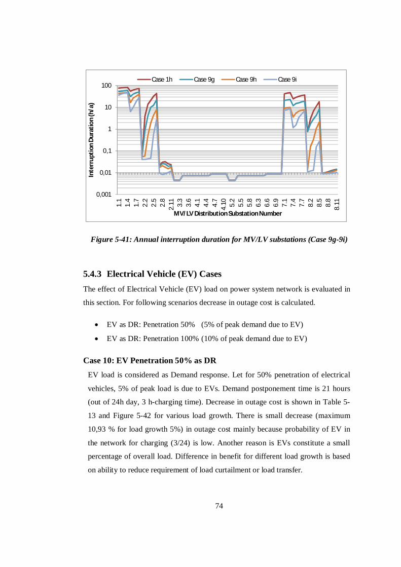
74


5.4.3 Electrical Vehicle (EV) Cases The effect of Electrical Vehicle (EV) load on power system network is evaluated in

this section. For following scenarios decrease in outage cost is calculated.

EV as DR: Penetration 50% (5% of peak demand due to EV)

EV as DR: Penetration 100% (10% of peak demand due to EV)

Case 10: EV Penetration 50% as DR

EV load is considered as Demand response. Let for 50% penetration of electrical

vehicles, 5% of peak load is due to EVs. Demand postponement time is 21 hours

(out of 24h day, 3 h-charging time). Decrease in outage cost is shown in Table 5-

13 and Figure 5-42 for various load growth. There is small decrease (maximum

10,93 % for load growth 5%) in outage cost mainly because probability of EV in

the network for charging (3/24) is low. Another reason is EVs constitute a small

percentage of overall load. Difference in benefit for different load growth is based

on ability to reduce requirement of load curtailment or load transfer.

0,001

0,01

0,1

1

10

100

1.1

1.4

1.7

2.2

2.5

2.8

2.11 3.

33.

64.

14.

44.

74.

10 5.2

5.5

5.8

6.3

6.6

6.9

7.1

7.4

7.7

8.2

8.5

8.8

8.11

Inte

rrup

tion

Dura

tion

(h/a

)


Case 1h Case 9g Case 9h Case 9i

75

Table 5-13: Decrease in Outage Cost due to EV load (Case 10)

Load Growth

(%)

Outage Cost with capacity Increase (€/a)

Outage Cost without Capacity

Increase (€/a)

Outage Cost considering EVs

(€/a)

Decrease in Outage Cost

(%)

5 4 260,36 87 643,05 78 525,42 10,93 10 4 463,24 372 946,10 336 516,50 9,89 15 4 666,11 827 756,15 760 337,51 8,19 20 4 868,99 1 591 934,35 1 461 675,60 8,21 25 5 071,86 2 626 270,67 2 411 499,35 8,19 30 5 274,74 3 766 802,25 3 472 360,61 7,83 40 5 680,49 6 480 238,22 5 981 353,95 7,71 50 6 086,24 9 486 861,76 8 742 095,45 7,86

Figure 5-42: Decrease in Outage Cost due to EV load (Case 10)

CASE 11: EV Penetration 100% as DR

Similar to case 10, EV load is considered as Demand response. Let for 100%

penetration of electrical vehicles, 10% of peak load is due to EVs. Demand

postponement time is 21 hours (out of 24h day, 3 h-charging time). Decrease in

outage cost is shown in Table 5-14 and Figure 5-43 for various load growth. There

is small decrease (maximum 12,5 % for load growth 5%) in outage cost mainly

0

2

4

6

8

10

12

5 10 15 20 25 30 40 50

Decr

ease

in O

utag

e Co

st (%

)

Load Growth (%)

% Decrease in OC Considering EV's

76

because probability of EV in the network for charging (3/24) is low. Another

reason is EVs constitute a small percentage of overall load. Difference in benefit

for different load growth is based on ability to reduce requirement of load

curtailment or load transfer. Compared to case 10 only small improvement in

decrease in outage cost is observed, which is due to high EV penetration.

Table 5-14: Decrease in Outage Cost due to EV load (Case 11)

Load Growth

(%)


(€/a)

Outage Cost without Capacity Increase

(€/a)

Outage Cost considering EVs

(€/a)

Decrease in Outage Cost

(%)

5 4 260,36 76 782,72 67 720,80 12,50 10 4 463,24 335 120,68 295 210,70 12,07 15 4 666,11 744 875,12 662 312,58 11,15 20 4 868,99 1 431 375,94 1 284 462,96 10,30 25 5 071,86 2 370 927,49 2 137 364,52 9,87 30 5 274,74 3 419 794,30 3 098 782,01 9,40 40 5 680,49 5 916 489,93 5 406 858,50 8,62 50 6 086,24 8 692 092,68 7 977 678,09 8,22

Figure 5-43: Decrease in Outage Cost due to EV load (Case 11)

0

2

4

6

8

10

12

14

5 10 15 20 25 30 40 50

Decr

ease

in O

utag

e Co

st (%

)

Load Growth (%)

% Decrease in OC Considering EV's

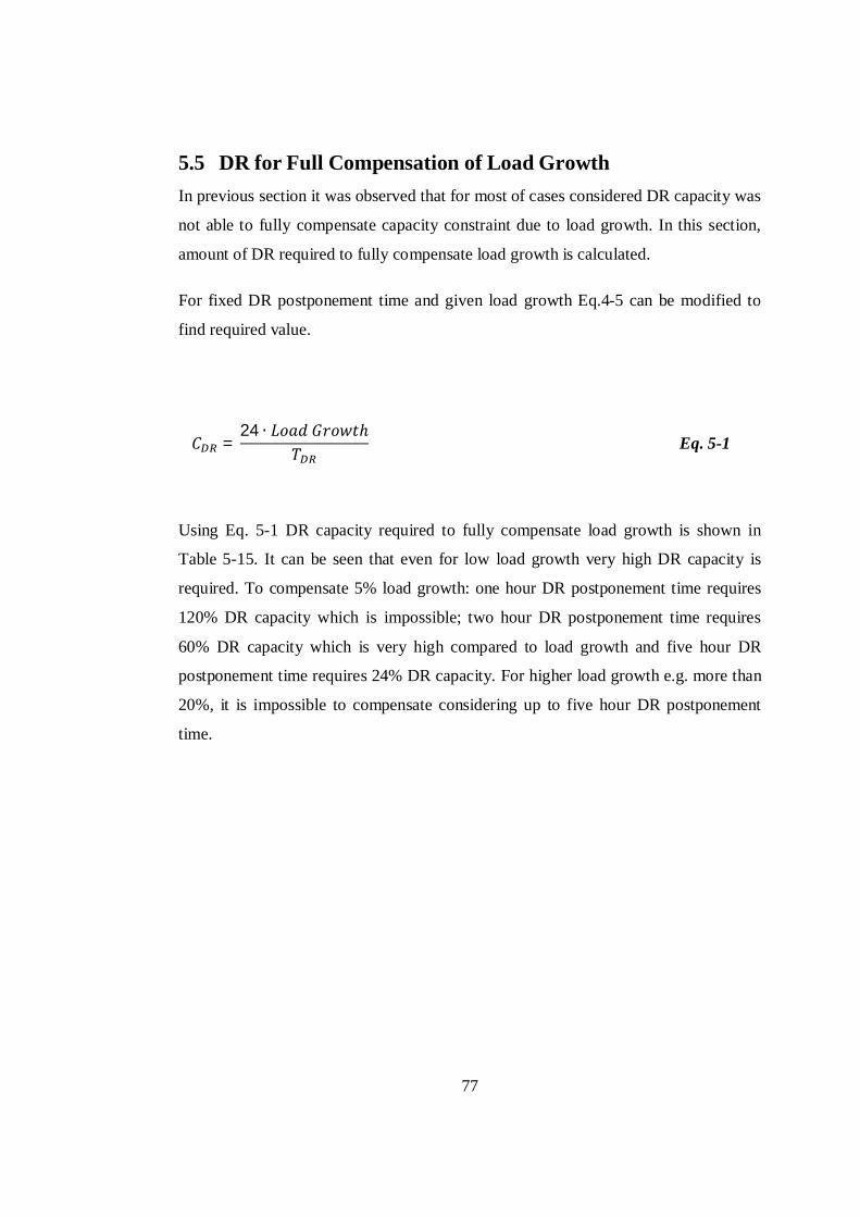
77

5.5 DR for Full Compensation of Load Growth In previous section it was observed that for most of cases considered DR capacity was

not able to fully compensate capacity constraint due to load growth. In this section,

amount of DR required to fully compensate load growth is calculated.

For fixed DR postponement time and given load growth Eq.4-5 can be modified to

find required value.

=24

Eq. 5-1

Using Eq. 5-1 DR capacity required to fully compensate load growth is shown in

Table 5-15. It can be seen that even for low load growth very high DR capacity is

required. To compensate 5% load growth: one hour DR postponement time requires

120% DR capacity which is impossible; two hour DR postponement time requires

60% DR capacity which is very high compared to load growth and five hour DR

postponement time requires 24% DR capacity. For higher load growth e.g. more than

20%, it is impossible to compensate considering up to five hour DR postponement

time.

78

Table 5-15: DR Capacity required for Full compensation of Load Growth.

Load Growth (%)

DR Postponement Time (h)

Required DR Capacity

(%) Comments

5 1 120 Impossible

5 2 60 5 5 24 10 1 240 Impossible

10 2 120 Impossible

10 5 48 15 1 360 Impossible

15 2 180 Impossible

15 5 72 20 1 480 Impossible

20 2 240 Impossible

20 5 96 25 1 600 Impossible

25 2 300 Impossible

25 5 120 Impossible

30 1 720 Impossible

30 2 360 Impossible

30 5 144 Impossible

40 1 960 Impossible

40 2 480 Impossible

40 5 192 Impossible

50 1 1200 Impossible

50 2 600 Impossible

50 5 240 Impossible

79

6 CONCLUSION AND FUTURE WORK

6.1 Conclusion The purpose of this thesis is to assess the possibility of reducing reserve requirement

of network components in the grid by Demand Response and Electrical Vehicles.

The method followed is; to consider load growth, calculate the outage cost without

investing into network, calculate the outage cost without investing into network

considering DR and EVs, then compare both the outage cost. Different load growth

and DR capacities are considered in the analysis.

For a particular load growth benefit of DR depends on DR capacity and

postponement time. Even for low load growth (e.g. 5%), to completely mitigate

reserve requirement, high capacity DR resources are required. Results are not

motivating, however, may be DR along with distributed energy resources (DER) can

make reasonable effect. These results can be used in estimating the advantage /

disadvantage of delaying investing in network, by comparing cost of adding

capacity and outage cost if capacity is not increased with load growth.

It can also be concluded that EVs are not feasible in mitigating the reserve

requirements of grid. The main reason is low probability of availability of EVs at

the time of requirement. Also Electrical Vehicles constitute only small portion of

overall load at grid. However, this does not mean EVs are not useful; these may be

helpful in other scenarios e.g. to store energy when excess quantity is available.

6.2 Future Work The analysis in thesis is conducted for single fault at a time and load point reliability

indices are calculated.

Analysis can be improved by considering effect of multiple contingencies.

Reliability indices at different system levels shall be calculated.

Distributed Energy Resources (DER) will be added in further study.

Load profile of EV’s will be included in future analysis.

80

REFERENCES

1. Fang Yang, “A Comprehensive Approach for Bulk Power System Reliability

Assessment”, Doctoral Dissertation, Georgia Institute of Technology, May

2007.

2. Jasper van Casteren, “Assessment of Interruption Costs in Electric Power

Systems using the Weibull-Markov Model”, Doctoral Dissertation, Chalmers

University of Technology, Göteborg, Sweden, 2003.

3. Sakis Meliopoulos and David Taylor and Chanan Singh, “Comprehensive

Power System Reliability Assessment”, PSERC report 05-13, April 2005.

4. Leonard L. Grigsby, “Electric Power Engineering Handbook Power Systems”,

CRC Press, May 30, 2007.

5. Marko C epin, “Assessment of Power System Reliability: Methods and

Applications”, Springer, August 4, 2011.

6. Richard E. Brown, “Electric Power Distribution Reliability”, CRC Press,

Second Edition, 2008.

7. Roy Billinton and Ronald N. Allan, “Reliability Evaluation of Power Systems”,

Plenum Press, Second Edition, 1996.

8. Marvin Rausand and Arnljot Hoylanc, “System Reliability Theory: Models and

Statistical Methods”, John Wiley & Sons, Inc., 2004.

9. R Billinton and R. Allan “Reliability Evaluation of Engineering Systems-

Concepts and Techniques” Plenum Press 1992 New York.

10. Markku Hyvärinen, “Electrical networks and economies of load density”,

Doctoral Dissertation, Helsinki University of Technology, Finland, 2008.

11. “Design Guide for Rural Substations, Issued June 2001, online available:

http://www.usda.gov/rus/electric/pubs/1724e300/1724e300.pdf

81

12. R. Billinton and Hua Chen and Jiaqi Zhou, “Generalized n+2 State System

Markov Model for Station-Oriented Reliability Evaluation”, IEEE Transactions

on Power Systems, Vol. 12, No. 4, November 1997.

13. Murty P. Bhavaraju and Roy Billinton, “TRANSMISSION SYSTEM

RELIABILITY METHODS”, IEEE Winter Power Meeting, New York, N.Y.,

January 31-February 5, 1971.

14. Robert J. Ringlee and Sheila D. Goode, “On Procedures for Reliability

Evaluations of Transmission Systems”, IEEE TRANSACTIONS ON POWER

APPARATUTS AND SYSTEMS, VOL. PAS-89, NO. 4, APRIL 1970.

15. J. Endrenyi, “Three-State Models in Power System Reliability Evaluations”,

IEEE Trans. Power Apparatus and Systems, Volume PAS-90, pp. 1909 - 1916,

July 1971.

16. Shahram Kazemi, “Reliability Evaluation of Smart Distribution Grids”, Doctoral

Dissertation, Aalto University, Finland, 2011.

17. IEEE Guide for Electric Power Distribution Reliability Indices, IEEE Standard

1366, New York, 2003.

18. IEEE Recommended Practice for Monitoring Electric Power Quality, IEEE

Standard 1159, New York, 2009.

19. U. S. Department of Energy, “Energy policy Act of 2005”, section 1252,

February 2006.

20. U. S. Department of Energy, “Assessment of Demand Response and Advanced

Metering Staff Report”, Docket AD06-2-000, August 2006 (Revised December

2008).

21. Michael R. Kleinberg and Karen Miu and Hsiao-Dong Chiang, “Improving

Service Restoration of Power Distribution Systems through Load Curtailment of

In-Service Customers”, IEEE TRANSACTIONS ON POWER SYSTEMS,

Volume 26, Issue 3, Aug. 2011.

82

22. L. Goel and Qiuwei Wu and Peng Wang, “Reliability enhancement of a

deregulated power system considering demand response”, IEEE Power

Engineering Society General Meeting, June 2006.

23. H. Aalami, G. R. Yousefi, and M. P. Moghadam, “Demand response model

considering EDRP and TOU programs,” in Proc. IEEE PES Transmission and

Distribution Conf. Expo., Apr. 2008, pp. 1–6.

24. Rahmat Azami, and Amir Faraji Fard, “Impact of Demand Response Programs

on System and Nodal Reliability of a Deregulated Power System”, ICSET, 2008

25. Salman Mohagheghi and Fang Yang and Bamdad Falahati, IEEE Power and

Energy Society General Meeting, July 2011.

26. P. Palensky and D. Dietrich, “Demand side management: Demand response,

intelligent energy systems, and smart loads”, IEEE Trans. Ind. Inform., vol. 7,

no. 3, pp.381 - 388, 2011.

27. Gustaf Nissen, “Cost Reduction Opportunities in Local Distribution Grids with

Demand Response”, Master’s thesis, Energy Systems Engineering at Uppsala

University, Sweden, June 2010.

28. U. S. Department of Energy, “Benefits of Demand Response and

Recommendations, Epact report”, February 2006.

29. Charles Goldman, “Grayson Heffner, and Michael Kintner-Meyer, "Do

Enabling Technologies Affect Customer Performance in Price-Responsive Load

Programs?”, August 2002, available online: http://certs.lbl.gov/pdf/50328.pdf

30. Seppo Kärkkäinen, “Demand Response activities in Finland”, DR Workshop

Copenhagen November 13, 2006.

31. Anna Cain and Iain MacGill and A. Bruce, “Assessing the potential impacts of

electricity vehicles on the electricity distribution network”, in Proc. 2010 the

48th Australian Solar Energy Society (AuSES), pp. 1- 10.

32. Trovao, L. and Jorge, H.M., “Power demand impacts of the charging of Electric

Vehicles on the power distribution network in a residential area”, Proceedings of

83

the 2011 3rd International Youth Conference on Energetics (IYCE), July 2011,

pp. 1- 6.

33. Aoife Foley, Brian O’Gallachoir and Ian Winning, “State-of the Art in Electric

Vehicles Charging Infrastructure”, in Proc. 6th IEEE Vehicle Power and

Propulsion Conference (VPPC'10), Lille, France, September 2010.

34. Marwan, M. and Kamel, F., “Optimum demand side response of Smart Grid

with renewable energy source and electrical vehicles”, 21st Australasian

Universities Power Engineering Conference (AUPEC), 2011, pp. 1- 5.

35. Wikipedia (2012), http://en.wikipedia.org/wiki/Electric_vehicle#Finland

(accessed 08 February 2012).

36. Website, http://askramadhan.wordpress.com/2009/03/22/busbar-configuration-

in-single-line-diagram/ (accessed 19 May 2012).

84

APPENDIX

Markov Process [8] A stochastic process satisfying the condition of Markov property is called Markov

process.

Markov property in words, if present state of process is given, the future state is

independent of previous states. Below is the equation form of Markov property

( ( + ) = | ( ) = , ( ) = ( ), 0 < )

= ( ( + ) = | ( ) = )( ), 0 <

Eq. 1 [8]

Where

{X(t), t 0} is continuous time stochastic process.

X = {0, 1, 2, … , r} is state space.

X(s) = State of process at time s is i.

Pr(X (t + s)) = j – Probability that the process will be in state j at time t + s.

{ x (u), 0 u < } is history of process.

The transitional probabilities of Markov process may be arranged in matrix form as

( ) =

( ) ( ) … ( )( ) ( ) ( )

( ) ( ) ( )

Eq. 2 [8]

Where P (t) = Pr(X(t) = j | X(0) = i) for all i, j X

85

The entries in row represents the transitions out of state ( ) , and entries in

the column represents the transition into state ( ). Since all the entities in

( ) are probabilities, so

( ) 1 0, , X

( ) = 1 Eq. 3 [8]

The amount of time spent in the state ( ) before making transition to other state is

exponentially distributed (rate= ). The mean sojourn time in state is

=1

The transition rate from state to is defined as

= Eq. 4 [8]

Since = 1, therefore

=,

Eq. 5 [8]

For a given a other two quantities and P can be found, thus a Markov process

can be defined by state space and transition rates. Transition rates arranged in matrix

form is called transition rate matrix of Markov process.

=

…

Eq. 6 [8]

86

For diagonal elements special notion used is given below

= =,

Eq. 7 [8]

Let is the time process spends in state before transition to state ( ). The

time is exponentially distributed with rate . Considering small time interval

we have

( ) = Pr =

( ) = Pr = 1

From these equations we find and

1 ( )=

<= Eq. 8 [8]

( )=

<= Eq. 9 [8]

By using Markov property and the law of total probability Chapman-Kolmogorov

equations are

( ) = ( ) ( )

Splitting interval (0, ) in two parts: transition from state to in small

interval (0, )and transition from state to in remaining interval. Now consider

( ) ( ) =,

( ) ( ) [1 ( )] ( )

Dividing by and taking limit as 0

87

( + ) ( )

=( )

,

( )

( ) Eq. 10 [8]

Since the summing index is finite, interchanging the limit and summation on the

RHS and using Eq.8 & Eq.9 along with ( ) = ( ), we get Kolmogorov

backward equations.

( ) =,

( ) ( ) = ( ) Eq. 11 [8]

In matrix form

( ) = ( ) Eq. 12 [8]

Similarly Kolmogorov forward equations are

( ) = ( ) Eq. 13 [8]

Assuming initial state of process is ( = 0) . . (0) =

So (0) = 1 and (0) = 0

As initial state is known, notion ( ) may be simplified as ( ). The vector

( ) = [P (t), P (t), … , P (t)] denotes the distribution of process at time t. The new

form of equations from Kolmogorov forward equations will be

[ ( ) ( ) ( )]

…

= ( ) ( ) ( )

Eq. 14 [8]

88

Another form

( ) = ( ) Eq. 15 [8]

Since the sum of entries in each row in A is zero, matrix is singular. Consequently

above equations does not have unique solution. By using fact ( ) = 1 and

initial state, often solution can be found.

Considering steady state probabilities i.e.(t ): lim ( ) = tends to constant

thus derivative is zero. Hence

0 = Eq. 16 [8]

With = 1 and out of + 1 equations from above Eq. 16 steady state

probabilities can be calculated.

Visit Frequency:

By putting values for steady state situation Kolmogorov forward equations can be

written as

0 =,

=,

Eq. 17 [8]

89

The probability of departure from state j in the time interval (t, t + t) is

( ( + ) = ) ( ( ) = ),

= ( ( + ) = )|( ( ) = ),

· ( ( ) = )

= ( ),

· ( )

Eq. 18 [8]

For steady state (t ) frequency of departure from state is given as

=( ), ·

= Eq. 19 [8]

Similarly, the frequency of departure from state into is . Therefore, total

frequency of arrival into state is

=,

Eq. 20 [8]

Above two equations show that frequency of departure from state is equal to

frequency of arrival into state . Thus steady state visit frequency to state is

defined as

= =,

Eq. 21 [8]

90

Mean Duration Of Visit:

It is given as reciprocal of rate of exponentially distributed function.

=1

= 0,1, … , Eq. 22 [8]

By putting value of from visit frequency Eq. 21

= = 0,1, … , Eq. 23 [8]

potential of demand response in mitigating the reserve ...sgemfinalreport.fi/files/humayun dtyo...

Documents