posterior predictive analysis for evaluating dsge … predictive analysis for evaluating dsge models...
TRANSCRIPT

NBER WORKING PAPER SERIES
POSTERIOR PREDICTIVE ANALYSIS FOR EVALUATING DSGE MODELS
Jon FaustAbhishek Gupta
Working Paper 17906http://www.nber.org/papers/w17906
NATIONAL BUREAU OF ECONOMIC RESEARCH1050 Massachusetts Avenue
Cambridge, MA 02138March 2012
The views expressed herein are those of the authors and do not necessarily reflect the views of theNational Bureau of Economic Research. Jon Faust was supported by a fellowship from the Departmentof Economics, Johns Hopkins University.
NBER working papers are circulated for discussion and comment purposes. They have not been peer-reviewed or been subject to the review by the NBER Board of Directors that accompanies officialNBER publications.
© 2012 by Jon Faust and Abhishek Gupta. All rights reserved. Short sections of text, not to exceedtwo paragraphs, may be quoted without explicit permission provided that full credit, including © notice,is given to the source.

Posterior Predictive Analysis for Evaluating DSGE ModelsJon Faust and Abhishek GuptaNBER Working Paper No. 17906March 2012JEL No. C52,E1,E32,E37
ABSTRACT
While dynamic stochastic general equilibrium (DSGE) models for monetary policy analysis have comea long way, there is considerable difference of opinion over the role these models should play in thepolicy process. The paper develops three main points about assessing the value of these models. First,we document that DSGE models continue to have aspects of crude approximation and omission. Thismotivates the need for tools to reveal the strengths and weaknesses of the models--both to direct developmentefforts and to inform how best to use the current flawed models. Second, posterior predictive analysisprovides a useful and economical tool for finding and communicating strengths and weaknesses. Inparticular, we adapt a form of discrepancy analysis as proposed by Gelman, et al. (1996). Third, weprovide a nonstandard defense of posterior predictive analysis in the DSGE context against long-standingobjections. We use the iconic Smets-Wouters model for illustrative purposes, showing a number ofheretofore unrecognized properties that may be important from a policymaking perspective.
Jon FaustJohns Hopkins UniversityDepartment of EconomicsMergenthaler Hall 4563400 N. Charles StreetBaltimore, MD 21218and [email protected]
Abhishek GuptaNational Institute of Public Finance and Policy18/2, Satsang Vihar MargSpecial Institutional AreaNew [email protected]

1 Introduction
Dynamic stochastic general equilibrium (DSGE) models have come a long way. After
Kydland and Prescott (1982) demonstrated that a small DSGE model could match a
few simple features of the macro dataset, there ensued a 20-year research program of
adding both complexity to the model and data features to account for, and the models
gradually began to approximate some of the richness we see in the macroeconomy.
A watershed event came in 2003 when Smets and Wouters (2003) demonstrated that
the family of DSGE models had reached the point that it ‘fit’ 7 key variables about as
well as some conventional benchmarks. They explain their main contribution:
[Our results] suggests that the current generation of DSGE models with
sticky prices and wages is sufficiently rich to capture the time-series prop-
erties of the data, as long as a sufficient number of structural shocks is
considered. These models can therefore provide a useful tool for monetary
policy analysis in an empirically plausible setup. (2003, p.1125)
While the first sentence is arguably true, the second is a non sequitur. For example,
Sims (1980) famous critique of the 1970s models was more or less that those models
were highly problematic for policy analysis despite their fit. Perhaps surprisingly, the
debate over the adequacy of DSGE models recently rose to the level of a Congressional
hearing. Solow (2010) argued that the models were deeply deficient:
The national—not to mention the world—economy is unbelievably compli-
cated, and its nature is usually changing underneath us. So there is no
chance that anyone will ever get it quite right, once and for all. Economic
theory is always and inevitably too simple; that can not be helped. But
it is all the more important to keep pointing out foolishness wherever it
appears. Especially when it comes to matters as important as macroeco-
nomics, a mainstream economist like me insists that every proposition must
2

pass the smell test: does this really make sense? I do not think that the
currently popular DSGE models pass the smell test. (p.1)
Chari (2010), (p.7), agreed that “We do not fully understand the sources of the
various shocks that buffet the economy over the business cycle,” but testified that
“[Policy advice from DSGE models] is one ingredient, and a very useful ingredient, in
policy making.”
Of course, these views reflect a long standing schism in macro.
We set aside this familiar argument over whether the glass is virtually empty or
essentially full. To push the tired glass metaphor to the breaking point, we take the
view that there is a nontrivial amount of something in the glass, and argue for focusing
on just what we are being asked to swallow.
That is, we take it as given that the DSGE models may be of significant value for as-
sessing certain questions, of less value for other purposes, and downright misleading for
others. We seek to provide tools for discovering and documenting particular strengths
and weaknesses of the models as they pertain to the intended task of monetary policy-
making. Thus, we follow Tiao and Xu (1993), (p.640), in arguing for “. . . development
of diagnostic tools with a greater emphasis on assessing the usefulness of an assumed
model for specific purposes at hand rather than on whether the model is true.”1
This paper supports three claims:
First, while DSGE modelling has come a long way, there remain important omissions
and areas of coarse approximation that may be materially important for policymaking.
The models remain in an ongoing state of material refinement. We think this claim
should be entirely uncontroversial but documenting some particulars provides a basis
for the later illustrations of our inference tools.
Second, prior and, particularly, posterior predictive analysis can be valuable tools in
assessing strengths and weaknesses of the DSGE models. Predictive analysis was origi-
nally popularized by Box (1980) and has been extended in many ways. Our contribution
1see also, e.g., Hansen (2005).
3

is to adapt these tools to the DSGE context and illustrate their usefulness. Most no-
tably, perhaps, we adapt the discrepancy analysis of Gelman et al. (1996), which seems
to have gotten little use in macro, to analyze the causal channels in DSGE models.
While prior and posterior predictive analysis have been widely used in many areas,
these techniques have also been criticized as being inconsistent with coherent inference.
Our third claim is that standard criticisms of prior and posterior predictive analysis,
whatever their merits in other contexts, miss the point in the DSGE context. In practi-
cal terms, posterior predictive analysis can be viewed as a natural pragmatic Bayesian
response to a very murky inference problem. The essence of our argument is that, in
practice, the DSGE literature stands conventional Bayesian inference reasoning on its
head.
The three main points come in the next three sections. From a purely practical
standpoint, our main goal is to illustrate that posterior predictive analysis is a conve-
nient way to discover and communicate complex issues about these complicated models
work. The proof of convenience comes mainly in the using of the tool, of course. We
make our case for the practical merits in section 3, where we take a version of the iconic
Smets Wouters model and highlight several important strengths and weaknesses. Smets
and Wouters have been incredibly gracious in helping us complete this work.
2 Standard Approaches to Bayesian DSGE Mod-
elling for Monetary Policymaking
2.1 The Macro Modelling Problem
We take largely as given a basic knowledge of the monetary policymaking process and
of DSGE modelling for use in the policymaking process. We provide the following
sketch. The policymakers of the central bank meet periodically to assess changes to
the values of the policy instruments under their control—the policy interest rates and
4

other policy tools. Taking as given the view adopted at the last meeting, a major task
at this meeting is to process the information that has arrived since the last meeting.
This processing is complicated by a number of features of the problem. The po-
tentially relevant information set is high dimensional. While there is no consensus on
how high dimensional, the ongoing policymaking process closely monitors hundreds of
variables.2 Certain research supports the view that forecasts of relevant variables based
on datasets of, say, 70 or more variables outperform others3 and that large-scale subjec-
tive forecast processes that focuss on even broader information sets may do better still
(Faust and Wright (2009)). Further, there is a rich set of dynamic feedbacks among the
myriad potentially relevant variables. By general consensus, general equilibrium effects
involving the expectations of a large set of heterogeneous agents may be central to the
policymaking problem.4
The existing policy process relies on many more and less formal tools, but is ulti-
mately heavily judgmental. The goal in DSGE modelling is to build a new model to aid
in the process of interpreting incoming data, forecasting, and simulation of alternative
policies.
From a modelling standpoint, forecasting does not strictly require a structural
model—that is, a model with explicit causal channels. The simulation of likely out-
comes under alternative counterfactual policy assumptions does require a structural
model, as does the attribution of unexpected movements in incoming data to particular
causes. To fix ideas, a standard textbook example of the latter involves attempting
to sort out whether an unexpected rise in GDP growth is primarily due to supply or
demand shocks. As these two causes may have different implications for policy, much
policy analysis involves this sort of inference.
Ideally, then, we need a model with fully articulated causal structure of a very large
2For example, see the Federal Reserve’s policy meeting briefing materials that are now available athttp://www.federalreserve.gov/monetarypolicy/fomc historical.htm
3e.g., Bernanke et al. (2005a); Bernanke and Boivin (2003); Faust and Wright (2009); Forni et al.(2005); Giannone et al. (2004); Stock and Watson (1999, 2002, 2003, 2005).
4For example, policy is often described as expectations management. See, e.g., Bernanke et al.(2005b).
5

and complicated system where theory provides limited guidance on important aspects
of the dynamics. The final complication is that we have a single historical sample for the
process we are modelling, the world macroeconomy. The models will be specified and
refined on this familiar dataset. New information arrives only with the passage of time.
By general consensus, the historical sample is not large enough to definitively resolve
all important issues. The ongoing lack of consensus on basic questions in macro is clear
testament to the idea that our only available sample is not resoundingly informative on
all relevant policymaking issues.
2.2 Description of DSGE Modelling and the SW Model
The approach in DSGE modelling is to explicitly state the decision problems of groups
of agents—e.g., households and firms—including objective functions and constraints.
For example, households choose consumption (hence, saving) and labor supply to max-
imize a utility function. Firms choose investment and labor input to maximize a profit
function. Ultimately the solutions to these individual optimization problems, when
combined with overall adding up constraints, imply the dynamic behavior of the vari-
ables modelled. Given the complexity of the models, we generally end up working with
some approximation to the full model-implied dynamics—for example, a log-linear ap-
proximation to the deviations from some steady state implied by the model.
A key feature of this kind of modelling is that agents are forward looking. In the
simplest forms of the decision problems, forward looking agents immediately react to
news about future conditions, and adjust their behavior much more quickly than is
consistent with the available macroeconomic data. Thus, ‘frictions’ are added to the
decision problems in order to slow down what would otherwise be excessively jumpy
behavior by agents.
Our example model is a version of the SW model described in Smets and Wouters
(2007).5 The model is an extension of a standard closed economy DSGE model with
5Readers are referred to Smets and Wouters (2007) for a thorough explanation of the model equa-
6
sticky wages and sticky prices, largely based on Christiano et al. (2005). The model
explains seven observables, with quantity variables in real, per capita terms: GDP
growth, consumption growth, and investment growth, hours worked, inflation, real
wage growth, and a short-term nominal interest rate.
The model has a rich set of frictions—the Calvo friction for prices and wages, (exter-
nal) habit formation in consumption, partial backward indexation of prices and wages,
and adjustment costs on the level of investment. The seven structural shocks are inter-
preted as shocks to overall productivity, investment productivity, a risk premium, the
wage markup, the price markup, the monetary policy interest rate rule, and, finally,
a shock Smets and Wouters variously refer to as an exogenous spending or govern-
ment spending shock. We will call it a government spending shock. Typically in this
literature, the shocks follow mutually independent autoregressive processes of order 1
(AR(1)). This is also true in SW with some exceptions. The price and wage markup
shocks follow ARMA(1,1) processes (autoregressive-moving average processes with each
part of order 1). Further, the exogenous government spending process is correlated with
the overall productivity shock.6
Because we will focus on consumption as an example later, it is worth going into a
bit more detail on the consumption problem. Consumers are assumed to maximize the
expected value of a discounted sum of period utility given by,
Ut =
(
1
1− σc
(Ct − hCt−1)1−σc
)
exp
(
σc − 1
1 + σl
L(1+σl)t
)
where Ct is consumption at time t, Lt is labor hours at t and h, σc and σl are scalar
parameters. The consumption portion of the utility function has (external) habit per-
sistence parameterized by h and risk aversion parameterized by σc, the coefficient of
tions and frictions.6In particular,
εgt = ρgεgt−1
+ ηgt + ρgaηat
where ρg and ρga are parameters, and ηg and ηa are the exogenous innovations to government spendingand overall productivity and εgt is the exogenous spending at t.
7
relative risk aversion (CRRA). Larger values of h tend to imply that agents will be
more reluctant to change consumption.
2.3 Estimation
Explicitly Bayesian inference methods are now the norm in DSGE modelling. The
methods used are, at a general level, a straightforward application of what we will
call the plain vanilla Bayesian approach.7 In a nutshell, this approach requires data,
a parameterized model, and a joint prior distribution for the parameters of the model.
The model implies a likelihood function for the data, and the model and prior together
exhaustively characterize the state of knowledge of the researcher before the new data
arrive. The plain vanilla Bayesian scheme tells us how to update the view reflected in
the prior density in light of new information that arrives.
Specifically, call the data Y and the model Mθ, with parameter vector θ ∈ Θ. In
the DSGE case, the likelihood, L(θ|Y ), is implied by the specification of the economic
model.8
In general, the data for DSGE exercises tend to be taken from the standard macro
data set; the sample period tends to be the longest continuous sample for which data are
available and for which the structure of the economy is believed to have been reasonably
stable. This latter involves a judgement call. SW estimate the model using US data
from 1966Q1 to 2004Q4.
Often there are multiple choices to be made in choosing model-based analogs to
key quantities in the model. For example, analysts sometimes use only nondurables
plus services consumption as the measure of consumption, since the model does not
7Plain vanilla here describes the application of Bayesian principles to a plain vanilla context. Thisdoes not tell us what Bayesian principles imply in a richer context such as—we argue—the one describedhere.
8 Once one has specified the model and processes for the exogenous driving processes, the decisionproblems of the agents can be solved and this solution implies a likelihood function. Generally forcomputational reasons we use a log-linear approximation to the exact solution of the model where theapproximation is centered on a non-stochastic steady-state of the model. This approximation givesrise to a linear, vector ARMA structure for the dynamics of the model.
8

explicitly model durables. SW’s consumption measure includes durables.
The prior, p0 is a joint density for θ over the parameter space Θ. The conventional
prior used in DSGE modelling varies, but in general terms the formal prior is often
specified as a set of marginal distributions for each individual parameter. These are
taken to be independent, implying the joint distribution for the prior. Generally, some
natural support for each parameter is implied by economic principles, technical stability
conditions for the model, and/or earlier applied work. The prior is specified to be fairly
dispersed over this support. Through trial and error, the analyst may find regions of
the parameter space in which the model seems ill behaved in some way, and the support
is narrowed.
While the papers often contain arguments justifying the support of the prior and,
perhaps, where it is centered, we have seen no argument that the joint prior implied by
the independent specification of marginal priors for the parameters has any justification
or has any tendency to produce results that are consistent with any subjective prior
beliefs over the joint outcomes implied by the parameter choices. Indeed, we have good
reason to think otherwise.9
Given the state of knowledge reflected in what we will call the model+prior and the
new information in the sample, Y r, a straightforward application of Bayes’s law gives
us,
p1(θ) ≡ pr(θ|Y r) = κp0(θ)L(Yr|θ)
where κ is the constant that makes the integral of the expression on the right (with
respect to θ) integrate to one.
The prior and posterior densities for the two key consumption parameters are shown
in fig. 1. Both posteriors are centered at about the same place as the prior, but the
posteriors are considerably more peaked, indicating that the data are somewhat in-
formative. The habit persistence parameter is fairly large, suggesting that agents are
9Del Negro and Schorfheide (2008) illustrate this very clearly and propose a partial solution in theform of training samples. We take this up in the final section.
9

highly averse to changing consumption; the CRRA parameter is in the range that has
become conventional for estimates of models like SW on this sample.
2.4 Material Deficiencies, Omissions and Coarse Approxima-
tions
Given the size of the system being modelled and the current stage of understanding of
the relevant mechanisms and modelling techniques and related algorithms, it remains
the case that existing DSGE models involve coarse approximation to some economic
mechanisms believed relevant for policymaking and omit other such mechanisms en-
tirely. This is meant to be a description of the current state of development, not a
criticism. To motivate the remainder of the paper, it is useful to provide some detail
on the state of modelling.
Consider omitted mechanisms and phenomena. Most standard DSGE models do
not separately treat durable goods, inventories, or housing, despite conventional wis-
dom that these items play an important role in business cycles. Many experts believe
that credit spreads have important predictive content that might be important for pol-
icymaking (e.g., Gilchrist et al. (2009)), but defaultable debt is not modelled. Indeed,
until the crisis, the financial sector of standard models was entirely trivial; current ef-
forts are attempting to remedy this omission. This list of omissions could obviously go
much longer.
It is also true that the modelling of phenomena that are included in the model is
often best viewed as a coarse approximation relative to the best knowledge of specialists
in the particular area.
For example, important aspects of individual behavior toward risk is parameter-
ized by the coefficient of relative risk aversion. In the best tradition of microfounded
modelling, we might ask experts in individual behavior toward risk what values for this
parameter might be appropriate. Unfortunately, expert opinion is overwhelmingly clear
on one point: individual behavior toward risk is a rich phenomenon not well captured
10

by this single parameter.10 Many micro phenomena simply cannot be accounted for un-
der this assumption. Suppose we tell the expert we are viewing this as a representative
agent approximation to underlying behavior, but would still like guidance on the value.
The expert should then remind us that different values will be best depending on the
goals of the approximation: to fit the equity premium from 1889 to 1978, CRRA > 10
(Mehra and Prescott (1985)); to fit aggregate lottery revenue using these preferences
probably requires risk loving; to fit the reaction of consumption to changes in monetary
policy, probably some value not too far from one is appropriate.
As a description of individual behavior, the CRRA specification is a crude approxi-
mation. It is difficult to view the choice of the CRRA parameter value as anything other
than choosing how best to center the crude approximation for a particular purpose.
Analogous issues can be raised about the treatment of habits. At the individual
level there is little evidence for strong habits (Dynan (2000)), but strong habits in
the model seem to be needed to ‘fit’ the smooth evolution of aggregate consumption
data. Alternative explanations for the aggregate persistence include serially correlated
measurement error (Wilcox (1992)), aggregation biases (Attanasio and Weber (1993)),
and ‘sticky expectations’ (Carroll et al. (forthcoming)). The choice of a habit parameter
value cannot coherently be viewed as anything but choosing how best to center the
crude approximation for a particular purpose. We could do a similar analysis of crude
approximations in the labor market, investment, and the financial sector.
Finally, it also the case that the prior used in these analysis is far from the idealized
case in which the model+prior fully reflects the subjective views of the relevant analysts.
As Del Negro and Schorfheide (2008) note, there is no reason to suppose that taking
reasonable marginal priors for the parameters and treating these as independent will
lead to reasonable general equilibrium implications for the model as a whole. As we
shall see below, it is not difficult to find examples where the prior is highly informative
and at odds with conventional wisdom.
10For a good review, see Camerer (1995).
11
Our goal here is only to put some concrete meaning to the claim that the models
continue to have areas of omission and crude approximation that may be relevant for
policy making. An alternative way to make this point is simply to cite the revealed
preferences of modelers at central banks. The models remain in a state of substantial
ongoing refinement and revision.
3 Prior and Posterior Predictive Analysis
The plain vanilla scheme described above tells us how optimally to shift our views on
the relative plausibility of different parameter values θ ∈ Θ. But it can never cast
doubt on whether the model as whole, Mθ, θ ∈ Θ, is adequate. In many contexts, this
might be troubling—George Box famously reminds us, all models are wrong–but it is
particularly troubling in a context where we are using an ad hoc prior over a model
with materially important aspects of approximation error and omission.
Box popularized a family of tools for checking whether an admittedly wrong model
might be useful based on prior and posterior predictive analysis. Box’s ideas have been
elaborated in a number of ways in the statistics and economics literature.11
In this section, we set aside conceptual criticisms of the approach, and illustrate the
way posterior predictive analysis can be used to highlight strengths and weaknesses of
DSGE models.12 The basic analytics of prior and posterior predictive analysis are all
well established in the statistics literature. Our contribution is to adapt these tools in
ways particularly useful in DSGE work.
3.1 Prior and Posterior Predictive Analysis Defined
Predictive analysis relies on simple idea: if the available sample is too freakish from the
standpoint of the model+prior or model+posterior, then perhaps the model or prior
11For example, Geweke (2005, 2007, 2010); Bernardo (1999); Gelman et al. (1996); Lancaster (2004).12It might seem more natural to give the theoretical justification before the applications. Our
theoretical arguments, however, turn on unique practical aspects of the DSGE context that are bestdiscussed after seeing some concrete examples.
12

should be refined.13
The essence of the argument can be seen in a simple example. We are considering
building a dam 6 meters high, but would like to know the probability that peak water
levels will overtop the dam in any given year. We have 50 annual observations on peak
annual water level. Our model states that the draws are independent and identically
distributed (iid) draws from a Gaussian distribution with unknown mean and variance
one. Our prior for the mean is uniform on [3, 4] meters. We draw a histogram of the
sample (fig. 2(a)) and notice that it is highly skewed to the right. This is disturbing
for a couple of reasons. It seems as if such a sample might be very unlikely to arise if
our peak water levels were really iid and Gaussian with constant mean. Further, the
particular way in which the sample is problematic is quite salient to our intended use
of the model: that excess mass in the right tail represents the cases in which the dam
is overtopped.
Of course, one sensible option would be to obtain another sample. But we are
imagining a case (like the macro modelling case) in which additional information will
only arrive slowly.
Predictive analysis provides a way to formalize the degree to which particular fea-
tures of the sample are peculiar. To perform the analysis, first we pick a formal data
feature to focus on. By data feature we mean any well-behaved function of the data:
h(Y ).14 Following the spirit in much macroeconomics one might think of these features
as empirical measures corresponding to some ‘stylized fact.’ In the example just given,
it would be natural to use the sample skewness as the data feature.15
The sample skewness for our sample is 1.05, whereas the population skewness of
13It might seem most natural to change the model, but in cases like DSGE modelling where theprior is substantially arbitrary, it is not unnatural to think of deciding that the arbitrary choice ofprior had put mass in ‘the wrong place.’
14Box called these model checking functions.15
h(Y ) =
T∑
t=1
(yt − y)3/(
T∑
t=1
(yt − y)2)3/2
where yt is the tth observation and y is the sample mean.
13
under the Gaussian maintained model is zero. However, one might wonder how likely
one would be to observe a sample skewness of 1.05 in a sample of size 50 if the sample
were in fact drawn from the model+prior at hand.
The model+prior imply a marginal distribution for any h(Y d), where Y d is a sample
of the size at hand drawn according to the model+prior:
Fh(c) ≡ pr(h(Y d) ≤ c) (1)
The function Fh is called the prior predictive distribution for h. One can plot the
implied prior predictive density, fh(c), along with the realized value h(Y r) for the sample
to get a sense of whether the realized value is freakish. Our example model+prior can
indeed produce samples with large positive and negative values for the sample skewness,
but would do so very rarely—the sample value of 1.05 is far in the tail of the predictive
distribution.
Where large values are considered unlikely, Box suggested a prior predictive p-value
defined as,
1− Fh(h(Yr)).
This is the probability of observing h(Y ) greater than the realized value in repeated
sampling if the data were generated by the model+prior. For our example, the p-value
is 0.003, or 0.3 percent.
There are, of course, dangers in summarizing a distribution with a single number
such as a p-value. Such crude summaries should be used with caution, and we will
largely report the entire predictive density. Still at times, p-values provide a convenient
and compact summary.
We can use the posterior distribution for the parameters of the model, p1, instead
of p0 in (1) in computing the predictive density, to obtain the posterior predictive
distribution and posterior predictive p-value. Once again, these predictive densities
depict the likelihood of observing specified sample features in repeated sampling from
14
the model+prior or model+posterior.
The features we have discussed so far are a function of Y alone. In modeling causal
channels we are not only interested in description, but in why events happen the way
they do. To shed light on causal channels, it is also useful to consider features that are
a function of the sample and θ: h(Y, θ). We will call the former ‘descriptive’ features
and the latter ‘structural’ features, to emphasize the dependence of the latter on the
structural parameter.
Gelman et al. (1996) have written extensively on what we call structural features.16
These seem to have received little application in macroeconometrics.
An example structural feature in the macro modelling case would be the sample
variance share of output growth attributed to demand shocks. Associated with any θ
there will be a population variance share of output attributed to demand shocks. On
any finite sample, however, demand or supply shocks might dominate. Using the model
to identify the shocks, we can then compute this sample variance share. Suppose we
find that demand shocks contributed 90 percent to the variance of output growth on
our sample. As with the sample skewness in the simple example above, we can ask
whether the model+prior or +posterior would be likely to produce a sample in which
demand shocks were this dominant.
There is an important complication, however, in the case of structural features.
Even after observing the sample, there is no single realized value on the sample at hand
since the true θ remains unknown. Gelman et al. note that conditional on any fixed
θ∗, we can compute h(Y r, θ∗) and, thus, could compute
pr(h(Y d, θ∗) > h(Y r, θ∗))
where Y d is a random sample of the same size as Y r drawn according to θ∗. Conditional
on θ∗, this corresponds to the p-value computed above. As always we can integrate out
16Gelman et al. call h(Y, θ) a discrepancy variable or simply discrepancy. The idea is that the featureis meant to help detect a discrepancy between the model and sample.
15
the dependence on the unobserved θ∗ using the prior or posterior to get, pr(h(Y d, θd) >
h(Y r, θd)), where θd is drawn according to the prior or posterior. This is analogous to
the p-value computed above.17
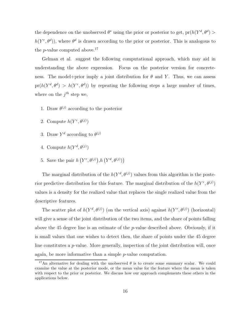
Gelman et al. suggest the following computational approach, which may aid in
understanding the above expression. Focus on the posterior version for concrete-
ness. The model+prior imply a joint distribution for θ and Y . Thus, we can assess
pr(h(Y d, θd) > h(Y r, θd)) by repeating the following steps a large number of times,
where on the jth step we,
1. Draw θ(j) according to the posterior
2. Compute h(Y r, θ(j))
3. Draw Y d according to θ(j)
4. Compute h(Y d, θ(j))
5. Save the pair h(
Y r, θ(j))
,h(
Y d, θ(j)))
The marginal distribution of the h(Y d, θ(j)) values from this algorithm is the poste-
rior predictive distribution for this feature. The marginal distribution of the h(Y r, θ(j))
values is a density for the realized value that replaces the single realized value from the
descriptive features.
The scatter plot of h(Y d, θ(j)) (on the vertical axis) against h(Y r, θ(j)) (horizontal)
will give a sense of the joint distribution of the two items, and the share of points falling
above the 45 degree line is an estimate of the p-value described above. Obviously, if it
is small values that one wishes to detect then, the share of points under the 45 degree
line constitutes a p-value. More generally, inspection of the joint distribution will, once
again, be more informative than a simple p-value computation.
17An alternative for dealing with the unobserved θ is to create some summary scalar. We couldexamine the value at the posterior mode, or the mean value for the feature where the mean is takenwith respect to the prior or posterior. We discuss how our approach complements these others in theapplications below.
16

Note that the predictive p-value for descriptive statistics can be computed using a
simplified version of the same algorithm exploiting the fact that h does not depend on
θ. Thus, the second step above may be computed outside the loop and the density for
the realized value collapses to a point. All we have to plot is the predictive density
and the realized point value. These are the algorithms we use in the examples reported
below.
3.2 Illustrations I: Descriptive Features
In this section, we illustrate how these techniques can be used to discover and highlight
strengths and weaknesses of DSGE models using the SW model. This is not intended
as a thorough substantive critique of this model; rather, we present examples meant to
illustrate the functionality of the methods and how they relate to methods commonly
used.18
It is useful to keep in mind two forms of analysis that are complementary to what we
are advocating: moment matching and full blown (Bayesian or frequentist) likelihood
analysis. In traditional moment matching with a DSGE model, one selects values for the
parameter, θ, and then compares population moments implied by the model to the cor-
responding sample moments for the sample at hand. In a full-blown Bayesian-inspired
likelihood analysis, the emphasis is on comparing models or parameter values based on
the relative likelihoods, perhaps, as weighted by the prior. We seek to emphasize how
posterior predictive analysis can be a complement to each.
In traditional moment matching in the DSGE literature, one might focus, say, on
standard deviations, correlations, and autocorrelations. In SW for example, the uncon-
ditional correlation of inflation and output growth at the posterior mode is -0.22, while
the corresponding sample correlation is -0.31. Based on the closeness of these two in
some informal metric, we might declare the model a success or failure.
18We provide a more complete analysis in other papers (Gupta (2010), Faust and Gupta (2010b),Faust (2009)).
17

These comparisons fail to represent two potential areas of uncertainty. First, sum-
marizing the model only by the correlation at a single θ does not reflect uncertainty
in the choice of parameter. Perhaps other similarly plausible θs imply very different
correlations. Replacing the single value of the correlation at the posterior mode θ with
a density implied by the posterior density for θ will bring the uncertainty in θ into the
comparison (fig. 3, dashed line). The solid line is the posterior density for the popu-
lation correlation implied by θ. Since the sample value is relatively far into the tail of
the posterior density, one might take this as evidence against the model.
There is a second aspect of uncertainty, however: the sample correlation is not
a precise estimate of the population correlation of the underlying process driving the
economy. Regardless of the population correlation, the model+prior could, in principle,
imply that any sample correlation might be likely to be observed in a small sample.
The posterior predictive density tells us what sort of values we would expect to see
for the sample correlation in repeated sampling with sample size equal to the sample
size at hand. It turns out (fig. 3, solid line) that under the model+posterior, there
is nothing particularly freakish about seeing sample correlations of -0.31 when the
population value is -0.22 at the posterior mode. In this case, the model is consistent
with the data essentially because the model+posterior imply that the sample correlation
will be poorly measured—correlations like that observed in the data are likely to be
observed even when the true correlation is substantially different.
Posterior predictive analysis of data features can also help examine the basic business
cycle properties of the model. For example, we could take as features the variance
shares of output growth occurring at business cycle frequencies. Early DSGE models
did not produce the persistent variation that is required to have a substantial share
of the variance in output occur at business cycle frequencies. In fig. 4, we report the
predictive densities for the output growth variance shares falling below, at, and above
business cycle frequencies.19 Both the posterior predictive densities are near the sample
19The business cycle region is bounded by periodicities of 8 and 40 quarters per cycle.
18
value in this case: from the standpoint of the model+posterior there is nothing freakish
about the sample distribution of variance across the spectrum. This is largely true for
the prior-predictive as well.20
Given that we are working with and refining a family of models with known ongo-
ing problems, posterior predictive analysis provides a way to investigate and highlight
known problem areas of the model. For example, the correlation of consumption and
investment growth in DSGE models has been a continuing problem. For most coun-
tries consumption and investment growth are strongly positively correlated: booms
and busts tend to involve both consumption and investment. There are forces in the
model, however, that tend to drive this correlation toward zero.21 In the SW model,
the posterior for this correlation is centered on low values (fig. 5, panel(a), solid line),
and the sample value of about 0.5 is far in the tail of the posterior. In this case, the
posterior predictive density is slightly more dispersed (fig. 5, panel(b), solid line), but
the p-value remains well below 1 percent. Formally, if samples were repeatedly drawn
from the model+posterior, less than 1 percent of draws would give values as extreme
as that observed on the sample.
In cases where the model+posterior suggest that the sample at hand is freakish,
there are three natural diagnoses: i) strange samples happen, ii) the model needs re-
finement, and iii) the prior needs refinement. This last possibility, of course, arises
particularly when the prior has ad hoc, yet highly informative, elements as is often the
case in the DSGE literature. To shed some light on this latter possibility we can look at
the prior predictive density. If the prior predictive density strongly favors low or nega-
tive correlations of investment and consumption growth, then the posterior result could
be due to the unfortunate choice of prior. In the current example, however, this is not
20The prior very strongly implies essentially no mass at lower than business cycle frequencies, whereasthe data want a bit of variance in this range. It is worth emphasizing that the estimate of the variancein this range is quite sensitive to the measurement method. Of course, we use the same measurementmethod on both the realized and predictive samples. But this should serve to emphasize that wheneverwe speak of a data feature, we should think of it as a feature measured in a particular manner.
21For example, a productivity shock that raises real interest rates may raise investment but reduceconsumption due to the increased incentive to save.
19

the case (fig. 5, panel(b), dashed line). The marginal prior for this sample correlation
actually favors large positive correlations.
For the SW model, the update using the data overpowered the prior and pushed the
posterior estimate to the far side of the sample value. This illustrates the complexity
of working with large general equilibrium, dynamic systems. The θs that give large
positive correlations of consumption and investment must have been down weighted
by the likelihood because those θs have some other implication that is at odds with
the sample. Smets and Wouters (2007, fn. 3) state that the risk premium shock is
included to help explain the correlation of consumption and investment growth. This
shock seems to do the trick in the prior, but not the posterior. We return to this issue
below.
These examples are intended to illustrate how posterior predictive analysis could
complement or extend the sort of moment matching exercises that have been common
in the literature.
Of course, defenders of full-blown Bayesian analysis have long criticized moment
matching. Looking at a few marginal distributions for individual moments is no sub-
stitute for a metric on the whole system, and the likelihood itself is the natural way
of summarizing the full implications of the model. Full likelihood analysis may show,
for example, that posterior odds favor, say, DSGE model A over DSGE model B. In
the analysis suggested by Del Negro et al. (2007), one forms a Bayesian comparison of
the DSGE model to a general time series model. In this case, one can learn that data
shift posterior plausibility mass along a continuum from the fully articulated structural
model to the general model with no causal interpretability. This sort of comparison
may be very useful as an overall metric on how the model is doing.
We are considering model building for ongoing, real-time policy analysis, however.
All the models have material deficiencies and are under ongoing substantial revision.
Thus, echoing our second and third main points from the introduction, we argue that in
addition to full-blown likelihood analysis it is important systematically to explore the
20

particular strengths and weaknesses of the model salient to the purpose of policymaking.
The fact that the posterior shifts mass from one model towards another is not very
revealing of the particular strengths and weaknesses of either. We argue that by using
a richer set of data features than simple moments, some important aspects of the models
can be revealed.
For example, Gupta (2010) argues that an important part of policy analysis at
central banks is interpreting surprising movements in the data. Policy at one meeting
is set based on anticipated outcomes for the economy. At each successive meeting,
policymakers assess how new information has changed the outlook and what this implies
for the appropriate stance of policy. In a formal model, this amounts to interpreting
the one-step (where a step is one decision making period) ahead forecast errors from
the model.
The simplest substantive example of this perspective comes in the textbook aggre-
gate supply/aggregate demand model. If prices and output come in above expectation,
one deduces that there has been an unexpected positive shock to AD. If output is
higher but prices lower than expected, one deduces that a favorable supply shock has
shifted aggregate supply. In the textbook case, the two outcomes have different policy
implications.
The key insight Gupta argues for is that policymakers need more than a model that
forecasts well in some general sense. They need a model that properly captures the joint
stochastic structure of the forecast errors. As a simple way to examine the properties
of the model in this regard, we can take our descriptive feature to be the correlation of
one-step forecast errors out of a benchmark time series model estimated on the sample.
For example, one could use a first order vector autoregression (VAR), a Bayesian VAR,
or a VAR with lag length set by AIC. All that is required is that based on the sample
alone, one can evaluate the value of the feature. For our illustration example, we use a
VAR with lag length chosen by AIC with length between 1 and 4. As features we take
21

the sample correlation of the one-step ahead forecast errors.22
Note that the model+prior very strongly favors correlations near one for the forecast
errors in real variables (fig. 6). Loosely, speaking, the prior seems to strongly favor
a world dominated by demand shocks as opposed to, say, productivity shocks that
would differentially affect the forecast errors. This illustrates the important lesson that
although the marginal prior distributions for the parameters are fairly dispersed, the
joint implications of the largely ad hoc prior for questions of interest in policymaking
may be highly opinionated and, indeed, concentrated in regions that conflict with true
subjective prior judgements. For example, no expert believes that if we could just
forecast output growth properly we could also nail a forecast for hours of work, but this
view is reflected in the model+prior used here (fig. 6(a), dashed line).23
It is also true that the realized one-step error correlations in these key quantity vari-
ables are quite unlikely from the standpoint of the model+posterior. In all three cases,
the realized value for the correlation is in the 0.5-0.6 range. For hours and output,
the model+posterior says values this low are moderately unlikely; for the other two
pairs, the model+posterior says values as high as that observed are unlikely. As with
the unconditional correlation, the investment-consumption pair is particularly prob-
lematic. In the sample, when investment was surprisingly high, consumption tended
to be surprisingly high as well. The model+posterior says these two errors should be
approximately uncorrelated.
The second row of fig. 6 gives the correlation of one-step errors of key quantity vari-
ables with the most closely associated price measure: consumption with general infla-
tion, hours with wage inflation, and investment with the interest rate. The model+posterior
suggests we should observe values near zero for the correlation error between surprises
in these pairs. For consumption and hours, however, on the historical sample, when
22Note: the one-step ahead errors are based on full-sample (not rolling) estimation and, hence,correspond to the OLS residuals.
23A complete diagnosis of this result is beyond the scope here. However, it appears that this is dueto the fact that all the shocks enter the prior with the same parameters. Despite being ‘the same’ inthis nominal sense, a given variance shock means something different economically depending on howit enters the model. In this case the result seems to be that the prior is that demand shocks dominate.
22
wage or price inflation was surprisingly high, the associated quantity tended to be
surprisingly low.
Once again, the literal meaning is that the sample is freakish from the standpoint
of the model+posterior. More provocatively, this literal interpretation means that
in practice on the realized sample, policymakers were systematically faced with the
problem of interpreting inflation and consumption growth surprises of opposite signs
(negative realized correlation in (fig. 6(d)). The model+posterior says that this pattern
was a freak outcome and policymakers need not worry much about facing this problem
in the future.
This simple example is only illustrative. Policymakers will in practice use a more
sophisticated forecasting model. Thus, one might ideally choose a more sophisticated
benchmark forecasting model. Or one could analyze the properties of optimal model-
consistent forecast errors. Gupta (2010) provides a version of this more complete anal-
ysis.
3.3 Illustrations II: Structural Features
Ultimately, policymakers must go beyond the descriptive in order to draw inferences
about the causes of economic variation and the likely causes of policy responses. Iden-
tifying causal structure in macro is very contentious, and when using a large model,
the problem is multiplied by the complexity of the system. It is very difficult to look
at a model and judge whether the causal structure as a whole is broadly consistent
with any given view. One natural way to focus the examination is to analyze what
‘causal story’ the model tells of the fluctuations in the familiar sample. In doing so, we
shift the large and amorphous question, ‘How does the model say the world works?’ to
‘What light does the model shed on the sample that is the source of current expertise
and conventional wisdom?’
In the current literature it is common to present a historical decomposition of head-
line variables like GDP growth in terms of the underlying structural shocks. Technically,
23

for any value of θ, we can compute our best estimate of the underlying latent struc-
tural shocks. Given the linear Gaussian structure assumed for the model, these can be
computed with the Kalman smoother24. The standard practice seems to be to produce
a historical decomposition in terms of the smoothed shocks evaluated at the posterior
mode for the parameter. For example, (fig. 7) taken from Smets and Wouters (2007)
shows that the SW model attributes much of the deep recession in 1982 to the collective
effect of demand shocks in the model. Demand shocks also account for much of the
recession in 2001.
These decompositions can be a very useful tool for understanding the models, but
we believe that posterior predictive analysis of structural features can form a valuable
complement to these historical decompositions. First, note that making judgments
about the model based on decompositions like this has the same problems that arise
in the simple moment matching discussed above: it ignores uncertainty in θ and if
some result seems amiss, it provides no systematic way to judge just how implausible
or freakish the result is.
There are many ways to use posterior predictive analysis to provide more systematic
results complementary to the historical decompositions. For example, for a broad overall
check we can take our structural feature, our h(Y, θ), to be elements of the sample
correlation or matrix of the smoothed estimates of the structural shocks.
Remember that all but one pair (government spending and overall productivity) of
structural shocks are assumed to be mutually uncorrelated in the model. The smoothed
structural shocks in a finite sample need not share this property. We can ask how-
ever, whether the sample correlation of the smoothed shock looks like it would if the
model+posterior were generating the data. As discussed above, this information is
contained in the joint distribution of h(Y (θ), θ) and h(Y r, θ), where θ is distributed
according to the posterior. To preview, under the model+posterior at hand, the distri-
bution of the sample correlation of smoothed structural shocks is generally symmetric
24Harvey (1991)
24
about zero, so the sample correlation of the smoothed structural shocks roughly share
the population property of the true structural shocks.
Consider the correlation of the smoothed productivity and investment productivity
shocks (fig. 8(a)). The posterior predictive (h(Y (θ), θ)) is plotted on the vertical axis,
the posterior distribution for the realized value on the horizontal. The point cloud is
a contour plot where the three rings of decreasing intensity moving outward cover 50,
75, and 95 percent of the mass, respectively. If we project the points leftward to the
vertical axis we would get the posterior predictive density for this correlation, which you
can see is more or less symmetric around zero—that is, the model+posterior says that
the correlation of the two smoothed shocks tends to be near zero and is very unlikely
to exceed ±0.2. Projecting down to the horizontal axis, we see that the posterior for
the correlation on the realized sample is centered around -0.3. The fact that there is
very little mass near the 45 degree line implies that there are no θs with appreciable
posterior mass for which we would be likely to see the large negative values computed
for the realized sample.
In economic terms, the model+posterior needed a large negative correlation between
the general and investment productivity shocks in order to account for the sample.
Before we discuss the economic interpretation, it is useful to observe a more complete
set of freakish correlations that the model needed (fig. 8).
The investment productivity shock showed freakish correlation with four other
shocks (panels a–d). The government spending shock also showed freakish correla-
tions with four shocks— investment productivity, monetary policy, price markup, and
risk premium (panels d–g). The risk premium shock showed freakish correlation with
the two policy shocks (government spending and monetary policy), the price markup
shock (panels g–i) and the investment productivity shock (panel b).
Diagnosing this full complement of freakish sample correlations is beyond the scope
of this paper. But a few comments are in order. What we are finding is closely related
to an argument of Chari et al. (2007). They measure certain wedges, which are closely
25
related to our one-step ahead forecast errors. They note that if two wedges (or one-step
errors) are positively correlated, then it must be that at least one structural shock moves
both wedges in the same direction. If the there is no such shock, then the model can
only accomodate the correlated forecast errors by finding that the underlying structural
shocks are correlated.
For example, suppose we have a simple AS/AD model driven by two demand shocks.
Both shocks move prices and quantities in the same direction on impact and tend to
cause the one-step ahead errors to be positively correlated. Suppose we estimate the
reduced form for the model on a given sample and find that the one-step forecast errors
for prices and quantities (on this sample) are negatively correlated. The model can
only accommodate this sample by finding that the two demand shocks (on this sample)
happened to be negatively correlated with a positive value of one demand shock pushing
up quantity at times when a negative realization for the other demand shock pushed
down prices. Of course, another interpretation of the finding of the negatively correlated
demand shocks is that the model is misspecified and needs a supply shock. Gupta
(2010) argues more fully how the correlations of the structural shocks and one-step
errors provide a road map for diagnosing structural misspecification.
Another alternative is to simply suspend the assumption of no correlation of the
structural shocks. Curdia and Reis (2010) explore this option. This correlation might
either be estimated as a diagnostic, in which case it is similar in spirit to what we are
doing,25 or it might be taken to be a serious structural alternative. Our main intent
is to develop a diagnostic and not to advocate a particular new structure. In general,
however, we think that if there is some systematic channel that would lead what we call
structural shocks to be correlated, then it makes more sense to model these channels
than to posit a correlation of shocks. For example, consider the correlation we find in the
monetary policy and government spending shocks. It is perfectly sensible to think that
25Note one clear difference. In our work the sample correlation we are detecting came as a surpriseto the agents, who believe that the underlying shocks are uncorrelated. Thus, the model is exploitingnot only a systematic correlation, it is exploiting a systematically surprising correlation.
26
monetary policy is surprisingly restrictive when government spending is surprisingly
high (panel e). This could be consistent with inflation targeting, for example, if high
government spending tended to portend inflation. Under this view, the correlation of
the ‘shocks’ is a symptom of a misspecification of the monetary policy rule in the model,
which should reflect this systematic reaction of policy to inflation caused by government
spending shocks. It would probably be more natural to fix the monetary policy rule
than to posit correlation of the exogenous shocks.
Let us consider an additional family of structural data features that highlight sta-
bilization policy, focussing on how the model helps us understand the recessions in the
sample. In the U.S., it is well known that periods of at least two consecutive quarters of
negative GDP growth correspond fairly closely to the NBER’s definition of recessions.
Thus, on any sample, we can partition the the smoothed structural shocks into those
occurring in an episode of at least two quarters of negative GDP growth and the others.
We can then examine the posterior predictive description that the model provides for
recessions.
For example, we can compute the sample standard deviation of smoothed structural
shocks in recessions and expansions, separately, and then compute the percent difference
in these two. Thus, a number like 0.2 means that the sample standard deviation of
shocks in recessions was 20 percent higher than that in expansions for the sample.
We find that under the model+posterior, we ought to expect to find about an equal
sample standard deviation of shocks in recessions and expansions That is, if we project
the points in the top row of fig. 9 to the vertical axis, we find that the distribution
of the difference is centered on zero. On the realized sample (projecting points to the
horizonal axis), however, we find that the shocks tended to be between 20 percent
and more than 60 percent larger in recessions than in expansions. The shocks were
consistently abnormally large in recessions on the realized sample—where abnormal is
relative to what the model+posterior are likely to produce.
In the second row of fig. 9, the feature is the simple difference in the correlation of
27

two referenced shocks during recessions versus expansions (recession minus expansion,
not in percentage terms). For each of the 4 pairs of shocks portrayed, the correlation
during recessions and expansions differed between 0.3 and 0.5 in absolute terms on
the realized sample. Under the model+posterior, the difference in correlations under
this partition of the observations should be about zero. Note that the correlation of
the government spending and risk premium shocks on the realized sample is around
0.5 higher in expansions than in recessions. This sample phenomenon is very strange
according to the model+posterior.
Overall, then, recessions in the post-War sample, according to the model, were
a collective freak occurrence of abnormally large and abnormally correlated shocks
occurring regularly with a periodicity corresponding roughly to that of business cycles.
Our goal in this section was to illustrate how posterior predictive analysis could be used
to find and illustrate important properties of DSGEmodels that might be relevant to the
model’s use in monetary policy analysis. In our view, some of the properties illustrated
are troubling from this standpoint, but we leave the substantive implications of our
illustrations to more systematic work.
It is important to note that there are many thorough critiques of this model, includ-
ing very incisive critique by the authors themselves, especially in joint work with Del
Negro and Schorfheide (Del Negro et al. (2007)). We argue that the sort of posterior
predictive analysis illustrated above provides a complementary tool and is especially
useful for highlighting strengths and weaknesses of the models as they pertain to par-
ticular uses such as policymaking.
3.4 Elaborations and Abuses
We have presented fairly straightforward illustrations in the previous section in order to
introduce these tools. There are many natural elaborations. For example, as Gelman
et al. note, one might want to condition all the computations on certain data features.
We have examined many different features and myriad others might be considered.
28

Whenever one has multiple statistics there are multiple ways they might be combined
and consolidated. For example, one could take account of the full joint distribution of
some group of features. Thus, one could ask how likely the model would be to produce
sample jointly showing values as extreme as the realized values. One could also combine
the features into some portmanteau feature and consider the marginal distribution of
the overall combined feature. We have argued for the benefits of interpretability of the
features and such a portmanteau would probably lose much of the interpretability.
Any discussion of the myriad features one might combine naturally leads to a dis-
cussion of how this approach might be misused and abused. On any sample, we can,
by examining the sample, discover features that are as ‘freakish’ as we like in the sense
of being present in a small proportion of all samples. Indiscriminate assessment of long
lists of features will, with probability one, lead us to discover that every random sample
(like every child) is special in its own way. As Gelman et al. (1996), Hill (1996) and
many others emphasize, any tool like this must be used with judgement. In particu-
lar, we are suggesting using these tools to highlight areas of consonance or dissonance
between the model and any strongly held views about the only existing sample.
As we raise this topic, however, we begin to squarely face the third major point of
the paper: our nonstandard defense to the standard criticisms of prior and posterior
predictive analysis.
4 Standard Criticisms and a Nonstandard Defense
of Posterior Predictive Analysis
While we believe that posterior predictive analysis could be an extremely useful tool,
uses so far in the DSGE literature have been limited. This may, in part, be because of
the strong arguments often stated against the coherence of this form of inference.
For example, Geweke (2010), (p.24), argues, while prior predictive analysis and pos-
terior predictive analysis are designed to uncover the same problems, “[T]he former are
29

Bayesian and the later are not.” Paired with Sims (2007) Hotelling lecture admonition
that “Econometrics should always and everywhere be Bayesian,” posterior predictive
analysis seems to face real problems.
In this section, we argue that standard arguments against posterior predictive
analysis—which have great merits in other cases—are moot or miss the point in the
DSGE context. Indeed, posterior predictive analysis is arguably a natural pragmatic
attempt to apply Bayesian principles under challenging conditions. While more coher-
ent approaches may be in the offing, we argue that posterior predictive analysis is at
least as coherent as the plain vanilla scheme if we start from an accurate description of
the inference problem.
4.1 Standard Criticisms
Prior and posterior predictive analysis like all inference based on hypothetical other
samples, violate the likelihood principle, which “essentially states that all evidence,
which is obtained from an experiment, about an unknown quantity θ, is contained in
the likelihood function of θ for the given data. . . ” (Berger and Wolpert, 1984, p.1).
Given that prior and posterior predictive analysis share with frequentist analysis an
emphasis on behavior in repeated sampling, many of the objections echo the arguments
in the familiar frequentist vs. Bayesian debate.
One cannot deny that troubling problems can arise whenever one attempts to cast
doubt on a model based on the fact that what was observed in the sample was less likely
than other samples that were not in fact observed.26 One way of seeing the problem of
casting doubt on a model due to the fact that the sample at hand is unlikely is that this
approach begs the question ‘unlikely compared to what?’ Absent a model that renders
the existing sample more likely, the argument goes, the fact that the sample is unlikely
under the current model is neither here nor there.
Inference without an explicit alternative is fraught a host of problems, leading some
26The literature here is immense. For a recent treatment aimed at economists, see Geweke (2010).
30

to the summary judgement (Bayarri and Berger, 1999, p.72), “The notion of testing
whether or not data are compatible with a given model without specifying any alter-
native is indeed very attractive, but, unfortunately, it seems to be beyond reach.”
Geweke (2010), (p.25), argues further that, while both prior and posterior predic-
tive analysis violate the likelihood principle, posterior predictive analysis involves “a
violation of the likelihood principle that many Bayesians regard as egregious.” This is
in part because this analysis uses the data twice in an important sense:27 one checks
the freakishness of the sample using the posterior that was already updated using that
same sample. As Geweke shows, this must blunt whatever evidence there is against the
model.
Berger and Wolpert (1984) offer the following summary judgement about the use of
such techniques:
Of course, even this use of significance testing [as proposed by Box] as an
alert could be questioned, because of the matter of averaging over unob-
served x. It is hard to see what else could be done with [the maintained
model] alone, however, and it is sometimes argued that time constraints
preclude consideration of alternatives. This may occasionally be true, but
is probably fairly rare. Even cursory consideration of alternatives and a
few rough likelihood ratio calculations will tend to give substantially more
insight than will a significance level, and will usually not be much more
difficult than sensibly choosing T [the data feature] and calculating the sig-
nificance level. (p.109)
We begin our defense of posterior predictive analysis by accepting (or, at least, not
contesting) essentially all of Berger and Wolpert’s points. In particular, until recently,
Berger and Wolpert’s claim that specifying explicit alternatives, perhaps in a cursory
manner, is easy was nearly a tautology. Until fairly recently, Bayesian methods were
27Without taking formal account of this fact
31

computationally infeasible except in nearly trivial cases and constructing cursory alter-
natives to trivial models is probably easy. Constructing meaningful alternative models
of the world macroeconomy with fully articulated causal channels, we argue, is not
easy. Thus, we claim that vDSGE modelling may be one of the rare cases envisaged
by Berger and Wolpert. We also agree with Berger and Wolpert that when one comes
across a rare case where specifying alternatives is not trivial, it is difficult to imagine
any systematic way to proceed other than some variant of the basic idea laid out by
Box, and that is what we are proposing. Our defense of posterior predictive analysis
goes considerably deeper.
4.2 Nonstandard Defense of Posterior Predictive Analysis for
a Nonstandard Context
Three features of the current context render much of the above argumentation es-
sentially moot. First, we have a single sample being used repeatedly. There is no
prospect of ‘fresh’ information as envisioned by the plain vanilla scheme. Second, the
model+prior do not even approximately conform to the ideal of summarizing all our
prior expertise before confronting ‘fresh’ information. Third, despite the state of mod-
elling, the current model is actively used in the policy process.
Perhaps the strongest way to put this is that in the standard scheme, the model+prior
are pefectly understood ex ante (before the update step) but the researcher is ignorant
of the sample ex ante. In practice, we are intimately familiar with the sample ex ante,
but the model+prior are very imperfectly understood. In an important sense, we use
a familiar sample to learn about an imperfectly understood model+prior, rather than
the other way around. Let us draw out these issues a bit.
One slowly growing sample. In DSGE modeling, macroeconomists are attempting
to formalize and reify our understanding of the world economy. Unfortunately, while
the available sample regarding the general equilibrium process is growing, it grows
32

sufficiently slowly that we may treat it essentially as fixed.28 Many rounds of refinement
take place using essentially the same data and, hence, the model, the formal prior and
the formal posterior in all DSGE work are deeply intertwined with the only existing
sample.
As in any progressive area, the posterior for the current model will soon be replaced
by another posterior, in this area the new posterior will be for a revised model informed
by the current sample, and this new ‘posterior’ will be computed on essentially the same
data as were the many previous versions.
For the remainder of this section by posterior (in italics) we simply mean what this
term has come to mean in the DSGE literature: the result of the latest round of update
on both the model structure and parameter values using the same sample as many
previous updates.
The fact of a single sample, raises other issues. Given the intertwining of professional
expertise and the only sample, it is almost inevitable that experts have certain strongly
held prior views regarding the current sample. For example, at the most general level,
most macroeconomists believe that regularly repeated features of the business cycle in
the familiar sample are in fact systematic features of the underlying mechanism and
not a freak outcome.
Posterior predictive analysis can be seen as a pragmatic way to check the consistency
of the model+posterior with difficult-to-impose prior views about the familiar sample.
The current model by general consensus remains materially deficient. As noted
above, Geweke argues that prior predictive analysis is consistent with Bayesian prin-
ciples but posterior predictive analysis is not. According to Geweke, this is because
prior predictive analysis can be confined to a specification analysis step that precedes
formal inference. In the specification analysis step, we confirm that the model+prior
are adequate, in some minimal sense. Then we proceed to formal inference.
28By general consensus (confirmed over the 30 year development process) the new information in afew observations is unlikely to provide much additional information. Observations like those from therecent crisis are arguably highly informative, but generally raise more questions than answers.
33

This is a coherent view and may be useful in many contexts, but it is highly prob-
lematic in the context of large-scale DSGE modelling. Under the Geweke construct,
we have been in the specification step for at least 30 years, and it appears that we will
remain in this step for the indefinite future. Of course, when the specification step is
done, we still will have no fresh sample on which to conduct formal inference. Thus,
even then, the two-step construct is problematic.
The current best model is actively informing policy. In the policymaking context, the
thought that formal inference is postponed indefinitely is especially problematic because
refinement of the deficient model goes on in parallel with actual decision making based
on the current best model. In lieu of a better alternative, the current model+posterior
will inform policy decisions.
There can be no doubt that the formal underpinnings of inference are murky at
best in this area with only one meaningful sample and a materially deficient model.
As an overarching idea, we think it is difficult to contest that if the current flawed
model+posterior will be used in policy analysis, then inspecting strengths and weak-
nesses of this model+posterior must be consistent with good sense as well as pragmatic
Bayesian principles.
4.3 An Alternative: Patch up the Plain Vanilla Scheme
In our experience discussing these issues, there is a very strong and proper urge to
consider the possibility that we could—perhaps in some cursory way as suggested by
Berger and Wolpert—paper over the difficult aspects of the DSGE context and restore
some scheme that has a reasonable pragmatic interpretation as being consistent with
the plain vanilla Bayesian scheme. Obviously, these suggestions involve methods to
eliminate ad hoc aspects of the prior and to accommodate in some way the most gross
deficiencies of the model.
For example, much of the problem stems from the idea of inference on model ad-
equacy without an alternative. In policymaking, there is an alternative to the DSGE
34

model: the implicit model embedded in the current subjective policymaking process. A
natural inclination might be to argue that we should render the current implicit model
to be formal and explicit, and then we can bring this newly formalized model into the
model evaluation. Of course, this misses the point entirely.
The current DSGE models built for policymaking are probably best thought of as
the current state of our efforts to reify the current wisdom in the policymaking process—
where by reify we mean to formalize the good and throw out the bad. Empirically, this
appears to be a multi-decade process. Our defense of posterior predictive analysis is
that this analysis can help render the process of reifying the model more efficient by
focusing attention on areas that are most troubling from the standpoint of the task at
hand.
There are other partial fixes that are promising. For example, Del Negro and Schorfheide
(2008) propose a useful approach to training samples as a method to reducing the sort
of problems with the conventional DSGE prior. We should be clear, however, that
deriving a prior based on a particular partitioning of the same information on which
the model has been specified and refined does nothing to restore the conventional plain
vanilla interpretation of the exercise. Indeed, there is no particularly strong reason to
use any given portion of the very familiar sample as the training as opposed to update
sample.29 It might be most natural to consider many such partitions in a sort of cross
validation. In any case, at the end of this process, posterior predictive analysis remains
a complementary tool for diagnosing issues in the model+posterior that result form this
process.
Geweke (2010) has recently published a brilliant book on working with complete and
incomplete econometric models, which involves methods for comparing explicit models
based on particular features and setting aside certain aspects of the model. This work
will undoubtedly find many important uses and will have important applications in
29For example, if you tell a well-informed macroeconomist which portion of the sample was used toinform the prior, the economist will have a strong ‘prior’ about what the update on the remainder ofthe sample will show.
35

DSGE modelling. For example, Geweke gives illustrations using trivial DSGE models
to address nonstructural questions (questions not involving policy counterfactuals).
Where applicable, we agree that such methods should be used.
Tools like these cannot overturn the fact that the complete general equilibrium
model and its implied causal structure are to be used in policymaking but nonetheless
have remaining deficiencies. We argue that under these conditions, any coherent class
of analysis must allow for the examination of the flaws of the current model+posterior
that is informing the policymaking process.
5 Conclusions
The modelling of causal channels in a large, dynamic system, with forward looking
behavior is an incredibly daunting task. It is made even more challenging by the fact
that we have a single dataset on which to both develop and test our theories. That
dataset is small—weakly informative—in materially relevant senses.
Perhaps it is not surprising in such a challenging context that there is little consensus
in the profession on key substantive economic topics or on modelling methodology.
The unprecedented Congressional hearing on DSGE modelling underscores both the
unfortunate state of affairs and the fact that improving on this state of affairs might
have immense welfare implications.
We argue for taking as a starting point that these models will actively be used in
policy analysis while remaining in an ongoing state of material refinement. Seen in this
light, posterior predictive analysis, we argue, can be a very useful tool for highlighting
strengths and weaknesses pertinent to policy.
We use the familiar Smets-Wouters model to illustrate these tools. The results
highlight that the prior used by Smets and Wouters is highly informative in certain
dimensions and some of these informative parts are grossly at odds with both the sample
and with conventional economic wisdom. DSGE models are often lauded because they
36

tell a full causal story for the sample. We illustrate what we think is the dominant
problematic aspect of the SW model’s story of post-War business cycles: according to
the model+posterior, business cycles of the variety observed were a regularly repeated
freak occurence. Taken literally, the main message to policymakers should be to prepare
for something else because the existing sample is dominated by repeated events that
will essentially never be repeated again. The alternative view we are advocating is that
the model+prior giving rise to the posterior are flawed in some way. Our tools help
investigate this possibility.
There are two overarching motivations for this type of analysis. First, it can help us
inform policymakers of limitations of the current models so that these limitations can
be judgementally allowed for in policymaking. Second, the analysis can help to direct
resources of the model refinement efforts to areas most relevant to policymaking.
37

Appendix
Raw inputs. We started with several inputs provided by Smets and Wouters: the
realized data, a posterior for θ as represented in 2 Markov chain Monte Carlo chains
with 263,810 draws, and the Dynare model code.
The prior. We took the prior as described in the dynare file provided by Smets and
Wouters. The prior that SW used, as defined in the model file we start with, has a few
minor differences from the one Smets and Wouters (2007) report in Table 1A and 1B.
Our prior calculations are based on 200,000 draws from the prior.
Prior and posterior calculations for features. For computing prior and posterior
predictive distributions we follow the algoritm given in the text. For posterior calcu-
lations, we are conditioning on the chains provided—e.g., taking these as comprising
the true posterior distribution. Thus, in implementing the algorithm stated in the text,
instead of taking some large number of random draws from the posterior, we evaluate
the features for each posterior draw provided in the chains. There is one potential
ambiguity in what was just described. In the MCMC chains, certain parameters are
‘drawn’ multiple times (that is, the algorithm remains on a certain θ for multiple steps).
If a given θ appears 4 times in the posterior chain, then we draw four samples for this
θ.
Details on features. Population correlation is based on the standard (first order)
approximation computed by dynare; the sample correlation is computed in the standard
way.
Variance shares in various frequency ranges are computed using a properly scaled
sum of the relevant periodogram points in each frequency range.
Recession quarters include any quarter in a span of at least two negative quarters
of GDP growth. Expansion quarters are all others. Recessions or expansions at both
ends of the sample are censored and no adjustment is made for this.
The smoothed structural errors are computed by Dynare. The Kalman filter is
initialized at the unconditional distribution implied by the θ at hand.
38

The VAR had a constant and all 7 variables. The lag length was chosen on each
sample using AIC with a maximum of 4 and a minimum of 1.
Smoothers. Our density plots are smoothed using a normal kernel function. The
contour clouds are smoothed as in Eilers and Goeman (2004).
39

References
Attanasio, O., Weber, G., 1993. Consumption growth, the interest rate and aggregation.
The Review of Economic Studies 60 (3), 631–649.
Bayarri, M., Berger, J., 1999. Comment on Bayarri and Berger. Bayesian Statistics 6,
53–67.
Berger, J., Wolpert, R., 1984. The likelihood principle. Institute of Mathematical Statis-
tics.
Bernanke, B., Boivin, J., 2003. Monetary policy in a data-rich environment. Journal of
Monetary Economics 50 (3), 525–546.
Bernanke, B., Boivin, J., Eliasz, P., 2005a. Measuring the effects of monetary policy:
A factor-augmented vector autoregressive (FAVAR) approach. Quarterly Journal of
Economics 120 (1), 387–422.
Bernanke, B., Reinhart, V., Sack, B., 2005b. Monetary policy alternatives at the zero
bound: An empirical assessment. Brookings Papers on Economic Activity 2004 (2),
1–100.
Bernardo, J., 1999. Quantifying surprise in the data and model verification. Bayesian
Statistics 6, 72–73.
Box, G., 1980. Sampling and Bayes’ inference in scientific modelling and robustness.
Journal of the Royal Statistical Society. Series A (General) 143 (4), 383–430.
Camerer, C., 1995. Individual decision making. The handbook of experimental eco-
nomics 3, 587–704.
Carroll, C., Slacalek, J., Sommer, M., forthcoming. International evidence on sticky
consumption growth. The Review of Economics and Statistics.
40
Chari, V., July 2010. Testimony before the U.S. House of Representatives. House Com-
mittee on Science and Technology, Subcommittee on Investigations and Oversight.
Chari, V., Kehoe, P., McGrattan, E., 2007. Business cycle accounting. Econometrica
75, 781–836.
Christiano, L., Eichenbaum, M., Evans, C., 2005. Nominal rigidities and the dynamic
effects of a monetary policy shock. Journal of Political Economy 113 (1), 1–45.
Curdia, V., Reis, R., 2010. Correlated disturbances and us business cycles. NBER
Working Papers.
Del Negro, M., Schorfheide, F., 2008. Forming priors for DSGE models (and how it
affects the assessment of nominal rigidities). Journal of Monetary Economics 55 (7),
1191–1208.
Del Negro, M., Schorfheide, F., Smets, F., Wouters, R., 2007. On the fit of New Key-
nesian models. Journal of Business & Economic Statistics 25 (2), 123–143.
Dynan, K., 2000. Habit formation in consumer preferences: Evidence from panel data.
American Economic Review, 391–406.
Eilers, P., Goeman, J., 2004. Enhancing scatterplots with smoothed densities. Bioin-
formatics.
Faust, J., 2009. The New Macro Models: Washing Our Hands and Watching for Ice-
bergs. Economic Review, 45–68.
Faust, J., Gupta, A., 2010b. Are all recessions black swans? DSGE models and the
post-war U.S. business cycle. in progress, Johns Hopkins University.
Faust, J., Wright, J., 2009. Comparing Greenbook and reduced form forecasts using a
large realtime dataset. Journal of Business and Economic Statistics 27 (4), 468–479.
41

Forni, M., Hallin, M., Lippi, M., Reichlin, L., 2005. The generalized dynamic factor
model. Journal of the American Statistical Association 100 (471), 830–840.
Gelman, A., Meng, X., Stern, H., 1996. Posterior predictive assessment of model fitness
via realized discrepancies. Statistica Sinica 6, 733–759.
Geweke, J., 2005. Contemporary Bayesian econometrics and statistics. John Wiley.
Geweke, J., 2007. Bayesian model comparison and validation. American Economic Re-
view 97 (2), 60–64.
Geweke, J., 2010. Complete and incomplete econometric models. Princeton Univ Pr.
Giannone, D., Reichlin, L., Sala, L., 2004. Monetary policy in real time. NBER Macroe-
conomics Annual 19, 161–200.
Gilchrist, S., Yankov, V., Zakrajsek, E., 2009. Credit market shocks and economic
fluctuations: Evidence from corporate bond and stock markets. Journal of Monetary
Economics 56 (4), 471–493.
Gupta, A., 2010. A forecasting metric for evaluating DSGE models for policy analysis.
in progress, Johns Hopkins University.
Hansen, B., 2005. Challenges for econometric model selection. Econometric Theory
21 (01), 60–68.
Harvey, A., 1991. Forecasting, structural time series models and the Kalman filter.
Cambridge Univ Pr.
Hill, B., 1996. Comment on Gelman, et al. Statistica Sinica 6, 767–773.
Kydland, F., Prescott, E., 1982. Time to build and aggregate fluctuations. Econometrica
50 (6), 1345–1370.
Lancaster, T., 2004. An introduction to modern Bayesian econometrics. Wiley-
Blackwell.
42
Mehra, R., Prescott, E., 1985. The equity premium: A puzzle. Journal of monetary
Economics 15 (2), 145–161.
Sims, C., 1980. Macroeconomics and reality. Econometrica: Journal of the Econometric
Society 48 (1), 1–48.
Sims, C., 2007. Bayesian Methods in Applied Econometrics, or, Why Econometrics
Should Always and Everywhere Be Bayesian. Hotelling Lecture, Duke University.
Smets, F., Wouters, R., 2003. An estimated dynamic stochastic general equilibrium
model of the Euro area. Journal of the European Economic Association 1 (5), 1123–
1175.
Smets, F., Wouters, R., 2007. Shocks and frictions in US business cycles: A Bayesian
DSGE approach. The American Economic Review 97 (3), 586–606.
Solow, R., July 2010. Building a science of economics for the real world. House Com-
mittee on Science and Technology, Subcommittee on Investigations and Oversight.
Stock, J., Watson, M., 1999. Forecasting inflation. Journal of Monetary Economics
44 (2), 293–335.
Stock, J., Watson, M., 2002. Forecasting using principal components from a large num-
ber of predictors. Journal of the American Statistical Association 97 (460), 1167–1179.
Stock, J., Watson, M., 2003. Forecasting output and inflation: the role of asset prices.
Journal of Economic Literature 41 (3), 788–829.
Stock, J., Watson, M., 2005. An empirical comparison of methods for forecasting using
many predictors. Manuscript, Princeton University.
Tiao, G., Xu, D., 1993. Robustness of maximum likelihood estimates for multi-step
predictions: the exponential smoothing case. Biometrika 80 (3), 623–641.
43

Wilcox, D., 1992. The construction of US consumption data: Some facts and their
implications for empirical work. The American economic review 82 (4), 922–941.
44

0 0.3 0.6 0.9 1.20
2
4
6
8
a) Habit Persistence0 1 2 3
0
2
4
6
8
b) CRRA
Figure 1: Prior and posterior densities for habit persistence and CRRA parameters(Dashed line: prior; solid line: posterior).
45
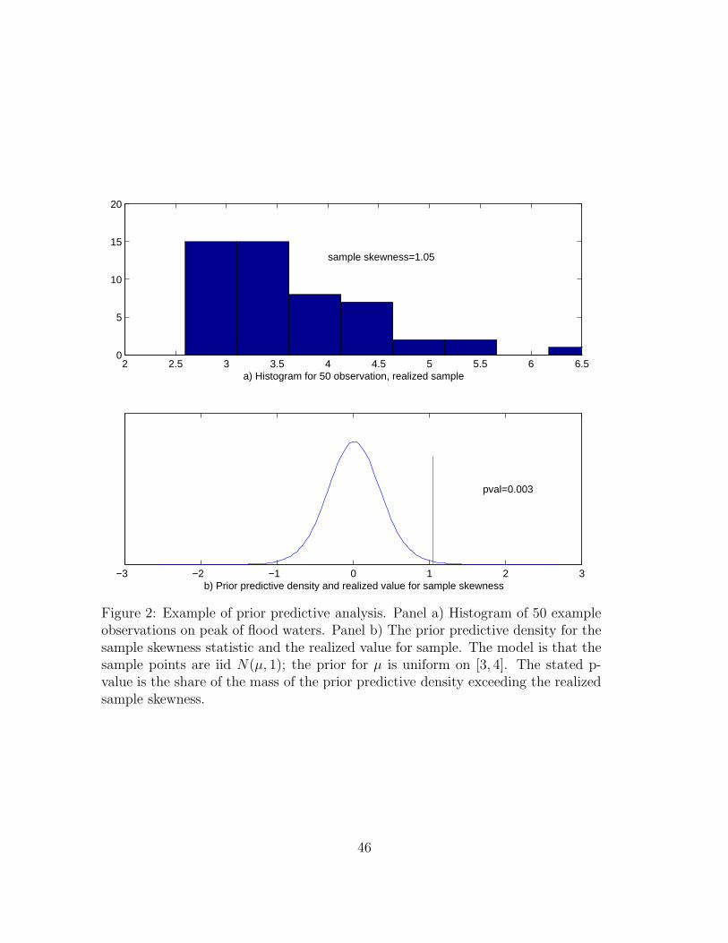
2 2.5 3 3.5 4 4.5 5 5.5 6 6.50
5
10
15
20
a) Histogram for 50 observation, realized sample
sample skewness=1.05
−3 −2 −1 0 1 2 3
pval=0.003
b) Prior predictive density and realized value for sample skewness
Figure 2: Example of prior predictive analysis. Panel a) Histogram of 50 exampleobservations on peak of flood waters. Panel b) The prior predictive density for thesample skewness statistic and the realized value for sample. The model is that thesample points are iid N(µ, 1); the prior for µ is uniform on [3, 4]. The stated p-value is the share of the mass of the prior predictive density exceeding the realizedsample skewness.
46
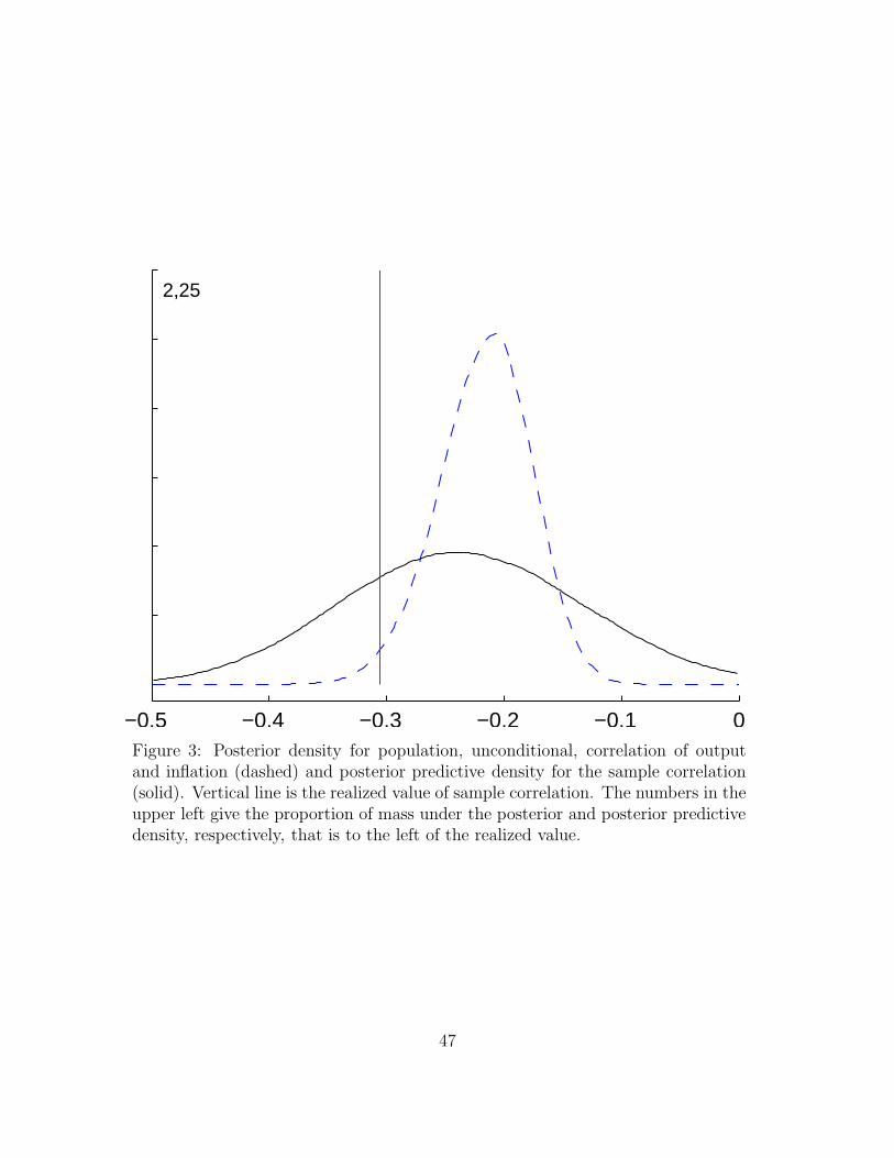
−0.5 −0.4 −0.3 −0.2 −0.1 0
2,25
Figure 3: Posterior density for population, unconditional, correlation of outputand inflation (dashed) and posterior predictive density for the sample correlation(solid). Vertical line is the realized value of sample correlation. The numbers in theupper left give the proportion of mass under the posterior and posterior predictivedensity, respectively, that is to the left of the realized value.
47
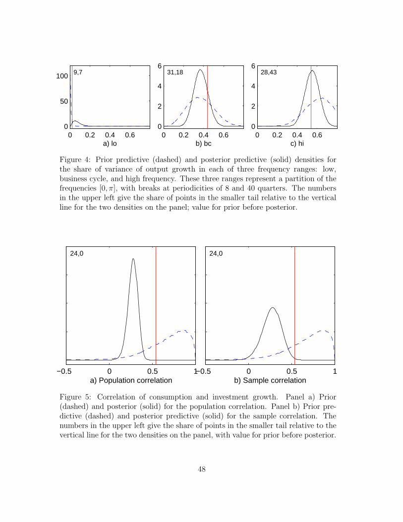
0 0.2 0.4 0.60
50
100 9,7
a) lo0 0.2 0.4 0.6
0
2
4
631,18
b) bc0 0.2 0.4 0.6
0
2
4
628,43
c) hi
Figure 4: Prior predictive (dashed) and posterior predictive (solid) densities forthe share of variance of output growth in each of three frequency ranges: low,business cycle, and high frequency. These three ranges represent a partition of thefrequencies [0, π], with breaks at periodicities of 8 and 40 quarters. The numbersin the upper left give the share of points in the smaller tail relative to the verticalline for the two densities on the panel; value for prior before posterior.
−0.5 0 0.5 1
24,0
a) Population correlation−0.5 0 0.5 1
24,0
b) Sample correlation
Figure 5: Correlation of consumption and investment growth. Panel a) Prior(dashed) and posterior (solid) for the population correlation. Panel b) Prior pre-dictive (dashed) and posterior predictive (solid) for the sample correlation. Thenumbers in the upper left give the share of points in the smaller tail relative to thevertical line for the two densities on the panel, with value for prior before posterior.
48

0
205,6
a) Y−h
7,4
b) Y−C
15,0
c) I−C
−0.5 0 0.5 1
0
4.53,1
d) C−pi−0.5 0 0.5 1
2,0
e) h−w−0.5 0 0.5 1
40,2
f) I−r
Figure 6: Sample correlation of one-step ahead forecast errors from VAR. Priorpredictive (dashed) and posterior predictive (solid) densities for one-step-aheadforecast error correlations. Vertical line is the realized value. The numbers in theupper left give the share of points in the smaller tail relative to the vertical line forthe two densities on the panel; value for prior before posterior.
49
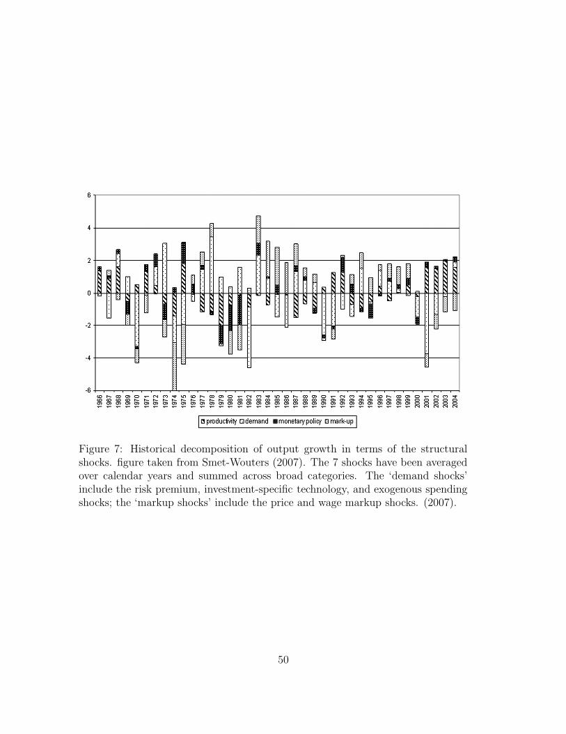
Figure 7: Historical decomposition of output growth in terms of the structuralshocks. figure taken from Smet-Wouters (2007). The 7 shocks have been averagedover calendar years and summed across broad categories. The ‘demand shocks’include the risk premium, investment-specific technology, and exogenous spendingshocks; the ‘markup shocks’ include the price and wage markup shocks. (2007).
50

0
a) ai−a−0.5
0
0.59
b) ai−rp
2
c) ai−wm
1
d) g−ai−0.5
0
0.53
e) g−mp
0
f) g−pm
0
g) rp−g−0.5 0 0.5
−0.5
0
0.56
h) rp−mp−0.5 0 0.5
0
i) rp−pm−0.5 0 0.5
Figure 8: Posterior predictive contour plots for the correlations of various struc-tural shocks. Each panel portrays the joint distribution of h(Y (θ), θ) (verticalaxis) and h(Y r, θ) (horizontal) where θ is distributed according to the posterior,Y comprises two structural shocks, and h is the sample correlation between thetwo shocks. The shock labels are: a, productivity, ai: investment productivity,rp, risk premium; pm: price markup; wm: wage markup; g: government spend-ing; mp: monetary policy. The number in the upper left is smaller of the shareof points on either side of the 45 degree line.
51

0
a) mp
−0.5
0
0.51
b) g
3
c) ai
0
d) rp
6
e) g−rp−0.5 0 0.5
−0.5
0
0.5 1
f) ai−rp−0.5 0 0.5
5
g) mp−ai−0.5 0 0.5
4
h) mp−wm−0.5 0 0.5
Figure 9: Posterior predictive contour plots for differences in properties of struc-tural shock in recessions and expansions. Each panel portrays the joint distribu-tion of h(Y (θ), θ) (vertical axis) and h(Y r, θ) (horizontal) where θ is distributedaccording to the posterior, Y is two smoothed structural shocks, and h is eitherthe the proportional difference (recession minus expansion over expansion) inshock standard deviation in the top row, and the simple difference in correla-tion (recession minus expansion) in the second row. The shock labels are: a,productivity, ai: investment productivity, rp, risk premium; pm: price markup;wm: wage markup; g: government spending; mp: monetary policy. The numberin the upper left is smaller of the share of points on either side of the 45 degreeline.
52