possibilistic analysis of arity-monotonic aggregation operators and its relation to bibliometric...

International Journal of Approximate Reasoning 52 (2011) 1312–1324

Contents lists available at ScienceDirect

International Journal of Approximate Reasoning

journal homepage: www.elsevier .com/locate / i jar

Possibilistic analysis of arity-monotonic aggregation operatorsand its relation to bibliometric impact assessment of individuals

Marek Ga�golewski ⇑, Przemysław GrzegorzewskiSystems Research Institute, Polish Academy of Sciences, ul. Newelska 6, 01-447 Warsaw, PolandFaculty of Mathematics and Information Science, Warsaw University of Technology, pl. Politechniki 1, 00-661 Warsaw, Poland

a r t i c l e i n f o a b s t r a c t

Article history:Available online 15 February 2011

Keywords:Aggregation operatorsPossibility theoryS-statisticsh-IndexOWMax

0888-613X/$ - see front matter � 2011 Elsevier Incdoi:10.1016/j.ijar.2011.01.010

⇑ Corresponding author at: Systems Research Inst+48 22 38 10 105.

E-mail addresses: [email protected] (M.

A class of arity-monotonic aggregation operators, called impact functions, is proposed. Thisfamily of operators forms a theoretical framework for the so-called Producer AssessmentProblem, which includes the scientometric task of fair and objective assessment of scien-tists using the number of citations received by their publications.

The impact function output values are analyzed under right-censored and dynamicallychanging input data. The qualitative possibilistic approach is used to describe this kindof uncertainty. It leads to intuitive graphical interpretations and may be easily appliedfor practical purposes.

The discourse is illustrated by a family of aggregation operators generalizing the well-known Ordered Weighted Maximum (OWMax) and the Hirsch h-index.

� 2011 Elsevier Inc. All rights reserved.

1. Introduction

In many areas of human activity like engineering, science, statistics, economy or social sciences, data summarization isoften required for further reasoning and decision making. A kind of synthesis of all individual inputs can be achieved byan appropriate aggregation.

Aggregation operators merge several numerical values into a single, representative one. Thus, from the perspective ofmathematics, aggregation operators are just projections from a multidimensional state space into a single dimension. Apartfrom particular applications, the theory of aggregation operators is a rapidly developing mathematical domain (we refer thereader to [1] for the recent state of the art monograph).

Most often, aggregation operators are considered for a fixed number of arguments. This might be too restrictive in someapplications. We face such situation in the so-called Producer Assessment Problem (PAP) described in Section 3, where givenalternatives are rated not only with respect to the quality of delivered items but also to their productivity. The issue of fairassessment of scientists based on the number of citations gained by their papers is the most representative instance of thePAP. The h-index proposed by Hirsch [2] is one of the most widely known tools used in this domain. This is the reason whyaggregation operators defined for arbitrary number of arguments are of interest.

The paper is organized as follows. In Section 2 we present the conventional notation used throughout the article and re-call some general information on aggregation functions and possibility measures. In Section 3 we describe the class of impactfunctions which form a model for the Producer Assessment Problem. Also we present some basic properties of impactfunctions.

. All rights reserved.

itute, Polish Academy of Sciences, ul. Newelska 6, 01-447 Warsaw, Poland. Tel.: +48 22 38 10 393; fax:

Ga�golewski), [email protected] (P. Grzegorzewski).

http://dx.doi.org/10.1016/j.ijar.2011.01.010

mailto:[email protected]

mailto:[email protected]

http://dx.doi.org/10.1016/j.ijar.2011.01.010

http://www.sciencedirect.com/science/journal/0888613X

http://www.elsevier.com/locate/ijar

M. Ga�golewski, P. Grzegorzewski / International Journal of Approximate Reasoning 52 (2011) 1312–1324 1313

Then, in Section 4, we study a class of aggregation operators, called the S-statistics [3,4]. These functions generalize theOrdered Weighted Maximum (OWMax) and the h-index.

In Section 5 we analyze the behavior of impact functions from a dynamic perspective, in which two possible situations aretaken into consideration. Firstly, some of the elements of the input vector may be likely to increase their values, e.g. whenpapers gain more citations. Secondly, we may also be faced with right-censored data, e.g. when we gather bibliometric re-cords from databases that do not cover the whole spectrum of journals, i.e. that underestimate the true number of citations.In both cases we are interested in predicting the effects of input vector alteration on the impact function’s output value. Herewe utilize possibility theory to express this kind of uncertainty. Our results are then illustrated in Section 6. Finally, Section 7summarizes the paper.

2. Preliminaries

2.1. Basic notation

Let I ¼ ½a; b� denote any nonempty closed interval of extended real numbers R ¼ ½�1;1�. The family of all subsets of I

will be denoted by PðIÞ. Unless stated otherwise, n;m 2 N. We assume that N0 ¼ f0;1;2; . . .g denotes the set of all nonneg-ative integers while [n] = {1,2, . . . ,n}.

Given any x ¼ ðx1; . . . ; xnÞ; y ¼ ðy1; . . . ; ynÞ 2 In, we write x 6 y iff ("i 2 [n]) xi 6 yi. Similarly, we say that x < y when x 6 yand x – y. Additionally, x ffi y iff there exists a permutation r of [n] such that (x1, . . . ,xn) = (yr(1), . . . ,yr(n)).

Let x(i) denote the ith-smallest value of x = (x1, . . . ,xn) and (n � x) the n-tuple ðx; x; . . . ; xÞ 2 In.The set of all vectors of arbitrary length with elements in I, i.e.

S1n¼1I

n, will be denoted by I1;2;.... For any x 2 In; y 2 Im andany function g defined on Inþm the notation g(x,y) stands for g(x1, . . . ,xn,y1, . . . ,ym).

2.2. Aggregation functions

To establish a point of reference for further discussion, let us first recall the notion of the aggregation function extended toany number of arguments. Here is the definition given in [1]. Note that much more restrictive sine qua non conditions wereproposed by Calvo et al. [5,6] by means of so-called a- and b-orderings.

From now on, let EðIÞ denote the family of all aggregation operators in I1;2;..., i.e. all the functions from I1;2;... to R. Thisdescription reflects the very general idea of data summarization/synthesis mentioned in the Introduction.

Definition 1. An (extended) aggregation function in I1;2;... is any function A 2 EðIÞ such that for any n

(A1) is nondecreasing in each variable, i.e. ð8x; y 2 InÞx 6 y) AðxÞ 6 AðyÞ,(A2) fulfills the lower boundary condition: infx2In AðxÞ ¼ a,(A3) fulfills the upper boundary condition: supx2In AðxÞ ¼ b.

Typical examples of aggregation functions are: the sample minimum, maximum, arithmetic mean, median, Bonferronimean [7], OWA [8] and OWMax [9] operators. On the other hand, the sample size, sum or any constant function generallyare not aggregation functions in the sense of Definition 1.

It is worth noting that axioms (A1) and (A2) imply A(n � a) = a. We also have A(n � b) = b by (A1) and (A3).The set of all extended aggregation functions in I1;2;... will be denoted by EAðIÞ.

2.3. Possibility theory

Let us recall here some definitions and concepts relevant to fuzzy measures that will be useful in further considerations.

Definition 2. A function l : PðIÞ ! ½0;1� is a fuzzy measure (also called normalized capacity) if

(a) l(;) = 0 and lðIÞ ¼ 1 (normalization),(b) for all A;B 2 PðIÞ, if A # B, then l(A) 6 l(B) (monotonicity).

Possibility theory is one of the formal representations of uncertainty. It may be used to describe the knowledge of anagent about the value of some quantity ranging on I; some states may be marked on a scale with ‘‘impossible’’ state onone side and ‘‘normal’’ or ‘‘unsurprising’’ on the other.

Definition 3. A fuzzy measure Pos is called a possibility measure iff for any family fAk 2 PðIÞ : k 2 Kg and an arbitrary indexset K,

Pos[k2K

Ak

!¼ sup

k2KPosðAkÞ: ð1Þ

1314 M. Ga�golewski, P. Grzegorzewski / International Journal of Approximate Reasoning 52 (2011) 1312–1324

With each possibility measure Pos we may associate another fuzzy measure Nec, called necessity measure, defined by

Table 1The Pro

ABCDE

NecðAÞ :¼ 1� Posð�AÞ; ð2Þ

where A 2 PðIÞ and �A denotes the complement of A. It may be shown that for every A 2 PðIÞ and for any possibility measurePos with the associated necessity measure Nec the following relations hold:

(a) Nec(A) > 0) Pos(A) = 1,(b) Pos(A) < 1) Nec(A) = 0.

Moreover, every possibility measure Pos is uniquely determined by a possibility distribution p : I! ½0;1�, i.e. for anyA 2 PðIÞ

PosðAÞ ¼ supx2A

pðxÞ: ð3Þ

The possibility distribution plays a central role in possibility theory. It represents the knowledge distinguishing what isplausible from what is surprising, e.g. p(x) = 0 means that x is considered impossible, while p(x) = 1 means that x is totallypossible. For more details concerning possibility theory, further references and other representations of uncertainty thereader is referred, e.g. to [10–14].

3. Impact functions and their properties

3.1. The Producer Assessment Problem

Consider a producer (e.g. a writer, scientist, artist, craftsman) and a nonempty set of his products (e.g. books, papers,works, goods). Suppose that each product is given a rating (of quality, popularity, etc.) which is a single number inI ¼ ½a; b�, where a denotes the lowest admissible valuation. Some typical examples of such situation are listed in Table 1.

It is clear that each possible state of producer’s activity can be described by a point in I1;2;.... The Producer AssessmentProblem (or PAP for short) involves constructing and analyzing aggregation operators which can be used for rating produc-ers [4]. A family of such functions should take into account the two following aspects of producer’s quality:

� the ability to make highly-rated products,� overall productivity.

Clearly, the first component can be properly described by a very broad class of (extended) aggregation functions (Defini-tion 1). However, note that any two restrictions AjIn and AjIm of an extended aggregation function A, where n – m, are gen-erally not necessarily related. Formally, we say that the family EAðIÞ is arity-free, i.e. ð8n – mÞ ð8fðnÞ 2 EAðIÞjIn Þ it holds

AjIm : A 2 EAðIÞ; AjIn ¼ fðnÞ� �

¼ EAðIÞjIm :

As stated above, in practice we are also interested in distinguishing between entities of different productivities. Therefore,we need some sine qua non requirements which should be satisfied by such assessing functions.

3.2. Impact functions

Consider the following definition. Its slightly modified version was given in [4].

Definition 4. An impact function in I1;2;... is a function J 2 EðIÞ; I ¼ ½a; b�, which

(I1) is nondecreasing in each variable: ð8nÞ ð8x; y 2 InÞx 6 y) JðxÞ 6 JðyÞ,(I2) fulfills the weak lower boundary condition: infx2I1;2;... JðxÞ ¼ a,(I3) fulfills the weak upper boundary condition: supx2I1;2;... JðxÞ ¼ b,

ducer Assessment Problem – typical examples.

Producer Products Rating method Discipline

Scientist Scientific articles Number of citations ScientometricsScientific institute Scientists The h-index ScientometricsWeb server Web pages Number of in-links WebometricsArtist Paintings Auction price AuctionsBillboard company Advertisements Sale results Marketing


(I4) is arity-monotonic, i.e. ð8n;mÞ ð8x 2 InÞ ð8y 2 ImÞ JðxÞ 6 Jðx; yÞ,(I5) is symmetric, i.e. ð8nÞ ð8x; y 2 InÞx ffi y) JðxÞ ¼ JðyÞ.

Conditions (I1) and (I4) correspond to the principle called ‘‘the more the better’’, which is justified in many practical in-stances of the PAP. According to (I5) each product is of equal importance and the overall rating is not affected by the pre-sentation order of the products.

Such formal model given for the PAP allows us to abstract from its context-dependent interpretation (to avoid any bias)and focus solely on the analysis of its mathematical properties.

The family of all impact functions will be denoted by EI ðIÞ. Note that the set of requirements given in Definition 4 is sim-ilar to the axiomatization proposed by Woeginger [15,16] for the so-called bibliometric impact indices (for other axiomati-zations see [17–20]).

It should be stressed that impact functions are not necessarily extended aggregation functions (in the sense of Definition1), because axioms (A2) and (A3) are replaced by their weaker forms (I2), (I3), respectively. For example, (A3) in conjunctionwith (I1), (I4), (I5) yields ð8x 2 InÞ ð9i 2 ½n�Þxi ¼ b) Jðx1; . . . ; xnÞ ¼ b, which generally is not a desirable property.

Moreover, (I1), (I4) and the closedness of I imply that (I2) is equivalent to the condition J(a) = a, and (I3) holds ifflimn?1J(n � b) = b.

3.3. Alternative definition

From now on, let P(I1) stand for the family of nondecreasing functions (i.e. functions satisfying axiom (I1) in Definition 4),P(I2) denote the functions fulfilling (I2), and so on. For example, P(A1) = P(I1), P(A2) # P(I2), P(A3) # P(I3) and EI ðIÞ ¼PðI1Þ \ PðI2Þ \ � � � \ PðI5Þ.

Consider the following relation E on I1;2;... which will be needed in further discussions. For any x 2 In and y 2 Im

x E y() n 6 m and xðn�iþ1Þ 6 yðm�iþ1Þ for all i 2 ½n�: ð4Þ

Of course, E is a partial order. Moreover, we write x / y if x E y and x – y.The following result is very important when considering the class of impact functions.

Theorem 5. Let F 2 EðIÞ. Then F 2 P(I1) \ P(I4) \ P(I5) if and only if ("x,y) x E y) F(x) 6 F(y).

Proof. ()) Let F 2 P(I1) \ P(I4) \ P(I5) and take any x E y; x 2 In; y 2 Im. We consider two cases.

(a) n = m. As ("i 2 [n]) x(i) 6 y(i), then by (I1) and (I5) it holds F(x) 6 F(y).(b) n < m. Let y0 ¼ ðyðmÞ; yðm�1Þ; . . . ; yðm�nþ1ÞÞ 2 In. By (I1) and (I5) we have F(x) 6 F(y0) and by (I4) F(y0) 6 F(y).

(�) Take any r;r0 2 S½n� and x 2 In. We have ðxrð1Þ; . . . ; xrðnÞÞ E ðxr0ð1Þ; . . . ; ðxr0 ðnÞÞ and ðxr0ð1Þ; . . . ; xr0ðnÞÞ E ðxrð1Þ; . . . ; xrðnÞÞ.Therefore Fðxrð1Þ; . . . ; xrðnÞÞ ¼ Fðxr0ð1Þ; . . . ; ðxr0ðnÞÞ and hence F is symmetric (axiom (I5)).

Now, take any x; y 2 In such that x 6 y. As x 6 y implies that x E y, we have F(x) 6 F(y) and so F is nondecreasing in eachvariable (axiom (I1)).

Lastly, for all x 2 In and any y 2 Im, (x) E (x,y), hence F(x) 6 F(x,y). Therefore F is arity-monotonic (axiom (I4)) and theproof is complete. h

Therefore, the class of impact functions is equivalent to the set of order-preserving maps (morphisms) from the partiallyordered set ðI1;2;...;EÞ to ðR;6Þ that fulfill (I2) and (I3).

3.4. Basic properties

Axiomatic modeling in decision making dates back to de Finetti [21], von Neumann and Morgenstern [22], Arrow [23](impossibility theorem in the problem of social states ordering) and May [24] (group decision functions).

Formally, a property P of functions in EðIÞ is an appropriate subset of EðIÞ.Below we discuss some basic properties which may be useful to describe the behavioral aspects of aggregation operators.

Some of them are desirable in particular instances of the PAP.

It can sometimes be justifiable to treat a ¼ min I as the ‘‘minimal admissible quality’’. Then adding new products withsuch rating should not affect the overall ranking (such elements are treated as negligible). By formalizing this idea we obtainthe following property.

Definition 6. We say that a function F 2 P(I2) \ P(I3) is a-insensitive iff F(x,a) = F(x) for any x 2 I1;2;....The family of a-insensitive functions will be denoted P(a0). By Definition 4 we get

Pða0Þ \ PðI1Þ # PðI4Þ \ PðI1Þ:


The above property may be strengthened as follows.

Definition 7. We say that a function F 2 P(I2) \ P(I3) is F-insensitive iff ð8x 2 I1;2;...Þ ð8y 2 IÞy 6 FðxÞ ) Fðx; yÞ ¼ FðxÞ.The family of F-insensitive aggregation operators will be denoted by P(F0). Note that if F 2 EIðIÞ then F 2 P(F0) iff

ð8x 2 I1;2;...ÞFðx;FðxÞÞ ¼ FðxÞ. We may also see that P(F0) # P(a0).On the other hand, in some applications it would be admissible that the function is sensitive for the addition of elements

greater that F(x).

Definition 8. We say that a function F 2 P(I2) \ P(I3) is F + sensitive iff ð8x 2 I1;2;...Þ ð8y 2 IÞ y > FðxÞ ) Fðx; yÞ > FðxÞ.The family of F + sensitive functions will be denoted by P(F+).For certain aggregation operators such a vector x may exist that any increment of the values of its coordinates never re-

sults in a change of the aggregator’s output. We say then that such operator is saturated at x. In this case only the addition(concatenation) of elements to x may increase the output value. Here is a formal definition of a saturable operator.

Definition 9. We say that a function F 2 P(I1) \ P(I4) is saturable (denoted F 2 P(sat)) iff ð8nÞ ð9x 2 In; x – n � bÞ ð8y 2 InÞ ifx < y then F(x) = F(y) and ð9z 2 Inþ1Þ FðzÞ > FðxÞ.

4. S-statistics

In this section we present a particular family of aggregation operators, called S-statistics (or ordered conditional maxi-mum). We then show which S-statistics are impact functions and in which cases the above-proposed properties are fulfilled.

For a different example of such analysis, we refer the reader to [4], where the class of L-statistics (or ordered linear com-bination), which generalize the ordered weighted averaging operator (OWA), is also considered.

Definition 10. A triangle of coefficients (compare [5,6]) is a sequence M ¼ ðci;n 2 I : i 2 ½n�;n 2 NÞ.Note that such object can be represented graphically by

c1;1

c1;2 c2;2

c1;3 c2;3 c3;3

..

. ... ..

. . ..

Definition 11. The S-statistic associated with a triangle of coefficients M ¼ ðci;n 2 I : i 2 ½n�;n 2 NÞ is a function SM 2 EðIÞsuch that

SMðxÞ ¼_ni¼1

ci;n ^ xðn�iþ1Þ ð5Þ

for x ¼ ðx1; . . . ; xnÞ 2 I1;2;..., where _ and ^ denote the supremum (and hence the name) and infimum operators, respectively.Without loss of generality we assume further on that ("n) c1,n 6 c2,n 6 � � � 6 cn,n. Actually, because if

Kn ¼ k ¼ 2;3; . . . ;n : ck;n 6_k�1

i¼1

ci;n

( )

then

_ni¼1

ci;n ^ xðn�iþ1Þ ¼_n

i¼1;iRKn

ci;n ^ xðn�iþ1Þ:

The Ordered Weighted Maximum operator (OWMax) defined for a fixed n, I ¼ ½0;1� and M such thatWn

i¼1ci;n ¼ 1 is anexample of a function SMjIn . It was first introduced in [9].

This extension of the OWMax operator to arbitrary number of arguments is analogous to the construction in [6,25] donefor OWA. For some general OWA operator weights construction methods see, e.g. [26,27].

The class of S-statistics was introduced in [4] as the ordered conditional maximum (OCM) operator. Some of its basic sta-tistical properties were examined in [3]. For instance, it turns out that for random input data (continuous i.i.d. random vari-ables) the distribution of an S-statistic is asymptotically normal.

It is worth noting that S-statistics generalize the well-known Hirsch h-index mainly used in the field of scientometrics.This index was originally defined in [2] for input vectors with elements in N0 as a function H such that

Hðx1; . . . ; xnÞ ¼ maxfi ¼ 0; . . . ;n : xðn�iþ1Þ P ig;

where we assume that x(n+1) = x(n). The h-index was proposed as a method of assessing the scientific merit of individualresearchers by means of the number of citations received by their scientific papers. It quickly received much attention in


the academic community [28,29]. Its popularity possibly arose from an appealing interpretation: the author of n papers hash-index of, say H, if H of his papers gained at least H, while the remaining n � H papers — at most H citations. Interestingly, asimilar object was defined earlier in the context of Bonferroni-type multiple significance testing (see, e.g. [30]).

For the expression of the h-index as a Sugeno integral (for more details compare [1]) of some function with respect to afuzzy counting measure see [31]. The next proposition is inspired by this result. Let N ¼ ðci;nÞi2½n�;n2N be the triangle of coef-ficients which may be represented graphically as follows:

11 21 2 3... ..

. ... . .

.

It may be easily shown (compare Theorem 14) that SN is an impact function in I ¼ ½0;1�.

Proposition 12. Let I ¼ ½0;1�. If N ¼ ðci;nÞi2½n�;n2N such that ci,n = i for n 2 N and i 2 [n]. Then for any m 2 N; x1; . . . ; xm 2 N0,

SNðx1; . . . ; xmÞ ¼ Hðx1; . . . ; xmÞ:

Proof. Let H = max{i : x(n�i+1) P i}. We haveWH

i¼1i ^ xðn�iþ1Þ ¼ H andWn

i¼Hþ1i ^ xðn�iþ1Þ ¼ xðn�HÞ < H þ 1. However, sincexðn�HÞ 2 N0, then x(n�H) 6 H and therefore

Wni¼1i ^ xðn�iþ1Þ ¼ H. h

Note that we have H(2,1.5) = 1 but SN(2,1.5) = 1.5. Generally, for arbitrary x, SN(x) = max{H,x(n�H)} 2 [H,H + 1) or, on theother hand, H(x) = bSN(x)c, where byc is the greatest integer 6y. Therefore H is equivalent to SN transformed by a particularnon-decreasing function.

One may be interested for which triangles of coefficients the S operator is an aggregation function and/or impact function.The answer is given in Theorem 14. However, for its proof we need the following lemma.

Lemma 13. Let I ¼ ½a; b� and n 2 N. Consider c; c0 2 In such that ci 6 cj and c0i 6 c0j for all i 6 j. Then we have

ð8x 2 InÞ_ni¼1

ci ^ xðn�iþ1Þ P_ni¼1

c0i ^ xðn�iþ1Þ () ð8k 2 ½n�Þ ck P c0k: ð6Þ

Proof. (�) Trivial.

()) Assume conversely. Let k be such that ck < c0k. Take any x ffi ðk � c0k; ðn� kÞ � aÞ. As c, c0 are nondecreasing, we haveWni¼1ci ^ xðn�iþ1Þ ¼ ck <

Wni¼1c0i ^ xðn�iþ1Þ ¼ c0k, a contradiction. Therefore the proof is complete. h

Additionally, it is easily seen that we have equality at the left side of (6) iff ð8k 2 ½n�Þ ck ¼ c0k.

Theorem 14. Let I ¼ ½a; b�. Then for any M ¼ ðci;nÞi2½n�;n2N; ci;n 2 I such that ci,n 6 cj,n for i 6 j we have

(a) SM 2 EAðIÞ iff ("n) cn,n = b,(b) SM 2 EIðIÞ iff ("n) ("i 2 [n]) ci,n+1 P ci,n P a and limn?1cn,n = b.

We omit the simple proof, which bases on the previous lemma and the fact that for arbitrary M always SM 2 P(I1) \ P(I5).We now characterize the S-statistics fulfilling the properties given in the previous section.

Proposition 15. For any I ¼ ½a; b� and any M ¼ ðci;nÞi2½n�;n2N; ci;n 6 cj;n for i 6 j, such that SM 2 EIðIÞ, the following holds:

(a) SM 2 P(a0) iff ("n) ("i 2 [n])ci,n+1 = ci,n.(b) SM 2 P(F0) iff SM 2 P(a0).(c) SM 2 P(F+) iff ("n) if c1,n < b then c1;nþ1 >

Wi2½n�;ci;n<bci;n.

(d) SM 2 P(sat) iff ("n)cn,n < cn+1,n+1 < b.

Sketch of the proof.

(a) It follows from the remark to Lemma 13.(b) Let us fix n. We should only show that ð8i 2 ½n�Þ

Wij¼1cj;n ¼

Wij¼1cj;nþ1 implies SM 2 P(s�). Let SM(x) = cj,n ^ x(n�j+1) for some

j. But as SM(x) 6 x(n�j+1) and xðn�jþ1Þ ^Wnþ1

i¼jþ1ci;nþ1 6 xðn�jþ1Þ, it holds SM(x,SM(x)) = cj,n+1 ^ x(n�j+2) = cj,n ^ x(n�j+1) = SM(x).


(c) Let us fix n and let cj;n ¼W

i2½n�;ci;n<bci;n for some j 2 [n]. Take x = (n � cj,n). Then for any e > 0SM(x,cj,n + e) > cj,n = SM(x) iffc1,n+1 > cj,n. Now take any y 2 In. Let SM(y) = cj,n ^ y(n�j+1) for some j. Then cj,n ^ y(n�j+1) < c1,n+1 ^ ((cj,n ^ y(n�j+1)) + e).

(d) SM(n � cn,n) = cn,n and ð8y 2 In : y > ðn � cn;nÞÞ SMðyÞ ¼ cn;n. There exists z 2 Inþ1 such that F(z) > F(x) iff b > cj,n+1 > cn,n forsome j 2 [n + 1] (z = ((n + 1) � cj,n+1)). But ci,n+1 6 cj,n+1 for i 6 j so it holds iff cn+1,n+1 > cn,n, and the proof is complete. h

For example, the generalized h-index, SN, is clearly an F-insensitive and saturable impact function.Moreover, the only SM 2 EIðIÞ which is both F-insensitive and F + sensitive is equivalent to the sample maximum (x(n)).

This is because for F-insensitive S-statistics we have c1,n = c1,m for all n < m. However, F + sensitivity requires that whenc1,n < b, then it should increase at c1,m. Therefore c1,n = b for any n. This indicates that the two properties together are toorestrictive.

5. Quality assessment in the dynamic perspective

5.1. Motivation

In this section we discuss a problem strongly related to ‘‘the more the better’’ principle of the PAP. To be more illustrativelet us focus our attention on the scientometric interpretation (Table 1A).

The problem is twofold. Firstly, perfect knowledge of the author’s publications and number of their citations is assumed.In practice we gather bibliometric data from large databases, such as Thomson Web of Science, Elsevier Scopus or Google Scho-lar (see, e.g. [32,33]). The coverage of digital libraries is limited, so in most cases we are dealing with right-censored data (see[29] for discussion). In other words, the true number of citations received by a paper is at least equal to the value obtainedfrom a given database.

Secondly, citations are merely an indicator of a paper’s quality as actually perceived by the scientific community. Everypaper, even the most influential one, has its initial number of citations equal to 0. That number grows as the work is recog-nized to be valuable (for some attempts to construct theories of citations in the social sciences see, e.g. [34–36]). Note thatthe acceptance of a paper for publication only expresses the fact this contribution meets at least some minimal journalstandards.

Therefore, we may say that the process of publishing and citing in its very nature is dynamic, i.e. an input vector x showsonly the current state of the producer and not its overall capability/potential. This state is very likely to change in the futureas he publishes more works and his papers gain more citations. This process itself is always accumulative as the statesx(1),x(2), . . . in consecutive time intervals form a chain w.r.t. the relation E, that is x(1)

E x(2)E � � �

Suppose someone described by x is applying for an academic tenure and he should determine his current impact F(x) forsome F 2 EI ðIÞ. Can he be sure that his rating is not about to increase shortly, due to the fact that some new papers citing hiswork will have been published before his application will be considered?

On the other hand, in case of saturable impact functions, the real values of input vector coordinates are sometimes ig-nored. Consider SN (discussed in Proposition 12) and I ¼ ½0;1�. The function value of SN(x) = 4 may be obtained for uncount-ably many x 2 I4: we have SN(x) = 4 iff x(n�3) P 4. However, it is not a sufficient condition for SN(x,5) = 5.

For another illustration let us consider the two vectors:

x ¼ ð4;4;4;4;0;0;0;0Þ; andy ¼ ð9;8;7;6;4;4;3;1Þ:

In both cases we have SN(x) = SN(y) = 4. However, not much is needed to increase SN(y) even to 6 (actually, some incrementsof y(3) and y(4) or appropriate element additions are only necessary).

Generally, given an impact function F 2 EI ðIÞ and a vector x 2 In we may try to raise the value of F(x) < b either by

(o1) increasing the value of some of the elements of x, i.e. finding y 2 In such that F(x + y) > F(x), or(o2) adding (concatenating) some elements to x, i.e. finding z 2 Im such that F(x,z) > F(x), or(o3) increasing the value of some of the elements and adding other elements simultaneously, i.e. finding y0 2 In and z0 2 Im

such that F(x + y0,z0) > F(x).

In each case some effort/cost (e.g. a publication of another paper, a marketing campaign) is required to improve the ratingof the producer described by x. However, one should be aware that there are impact functions and input vectors for whichsome of the above-mentioned actions do not result in the desired rating improvement. For example, in case of (o1), if F issaturable such y may sometimes not exist.

5.2. Effort-measurable functions

In this paragraph we distinguish a class of aggregation operators, called effort-measurable functions and its subclass,effort-dominable functions. Then we propose some general methods of creating possibility distributions that can help to


describe how the aggregation operator’s output value is likely to change when the above-mentioned operations (o1)–(o3)are applied to an input vector.

Let F 2 P(I1) \ P(I4) \ P(I5) and let VF ¼ F½I1;2;...� (the image of F). Moreover, for each v 2 VF let F�1½v � :¼ fx 2 I1;2;... : FðxÞ ¼ vgdenote the level set of v. (Note that, technically, in the level set we should retain only the elements that are unique w.r.t. therelation ffi to avoid ambiguities.)

Definition 16. We say that F 2 P(I1) \ P(I4) \ P(I5) is an effort-measurable function (denoted as F 2 P(em)) iff for every v 2 VF,(F�1[v], E) is a partially ordered set with a least element.

In other words, F 2 P(em) iff (F�1[v], E) is a bounded semi-lattice for all v 2 VF.Not all impact functions are effort-measurable. For example, some L-statistics, i.e. aggregation operators of the form

LMðxÞ ¼Pn

i¼1ci;nxðn�iþ1Þ, such that LM 2 EIðIÞ, do not belong to P(em).Let us denote the least element of F�1[v] by lv, i.e. lv = minF�1[v]. Moreover, let MF denote the set of all least elements

corresponding to level sets for all v, i.e. MF = {lv : v 2 VF}.For example, consider the impact function Max(x) = x(n). We have Max�1½v� ¼ fx 2 I1;2;... : xðnÞ ¼ vg and lv = minMax�1[v] = (v).

Definition 17. We say that an effort-measurable function F is effort-dominable (denoted as F 2 P(ed)) iff (MF,E) is a chain.

Every effort-dominable function F 2 P(ed) may be defined as follows. For any x 2 I1;2;...

FðxÞ ¼ maxlv2MF :lvEx

v;

hence for v,v0 2 VF we have lv / lv 0 () v < v 0.For example, the rp-indices discussed in [37,38] are effort-dominable. Their definition will be recalled in Section 6, see (8).Of course, not all effort-measurable functions are effort-dominable, e.g.

FðxÞ ¼ aþ ðb� aÞ=5 �max i ¼ 0; . . . ;minfn;4g : i ¼ 0 or xðn�iþ1Þ P 5� i� �

is a counterexample ðI ¼ ½a; b�; x 2 InÞ.Now we turn back to our exemplary class of functions. We check which of the S-statistics are effort-dominable and effort

measurable.

Proposition 18. Let M ¼ ðci;nÞi2½n�;n2N; ci;n 6 cj;n for i 6 j, such that SM 2 EI ðIÞ; I ¼ ½a; b�. Then the following conditions areequivalent:

(a) given any n and k = min{i:ci,n = cn,n} we have ("i < k) ci,n+1 = ci,n and ("j P k) cj,n+1 P ck,n,(b) SM is effort-dominable,(c) SM is effort-measurable.

Proof

(a) b) Let v 2 VSM ; n be the smallest number such that cn, n P v. For any m P n,

minfx 2 Im : SMðxÞ ¼ vg ffi ðkm � v ; ðm� kmÞ � aÞ;

for some km 2 [m] (min is w.r.t.E). ci,m = ci,n for i < kn and ckn ;m P ckn ;n implies that km = kn, so lv ffi (kn � v, (n � kn) � a)is the least element of S�1

M½v�. However, given arbitrary v 0 > v ;v 0 2 VSM , there exists n0 P n such that

ðkn � v ; ðn� knÞ � aÞ / ðkn0 � v 0; ðn0 � kn0 Þ � aÞ ffi lv 0 .
(b) c) By Definition 17.(c) a) Please note that for any effort-measurable operator SM 2 EIðIÞ we have lv ffi (k � v, (n � k)⁄a), where n = min{i :
ci,i P v} and k = min{i : ci,n P v}. ("m P n) ("i < k)ci,m < v, because otherwise SM(i � v, (m � i) � a) = v and lv 5 (i � v,(m � i) � a) which leads to contradiction.By Theorem 14, ci,n 6 ci,m < v 6 ck,n. However, considering any v 2 VSM , this statement implies ci,n = ci,m for i < min{j :cj,n = cn,n} and the proof is complete. h

Moreover, this result implies that SM 2 P(a0)) SM 2 P(ed).

5.3. Possibilistic approach

The modeling of complex processes underlying the changes of products’ ratings can hardly be described by stochasticmethods, even if we accept drastic simplifications and idealizations. Hence, we should try to develop approximate methodsthat can help to answer the question: Which input vectors are more likely to entail greater impact function values?


Thus our final goal is to establish a framework for some qualitative possibility relations between values of the impactfunction under study for different input data. Such possibility distribution functions might be useful for comparing the ef-fects of increment and/or addition of elements on the aggregation operator’s value.

Definition 19. An impact possibility distribution for an effort-measurable function F 2 P(em) is a mapping pF : I1;2;...�R! ½0;1� such that for any x 2 I1;2;... the following conditions hold:

(a) pF(x;F(x)) = 1,(b) if v < F(x) or v R VF then pF(x;v) = 0,(c) if x E y and v P F(y), then pF(x;v) 6 pF(y;v),(d) if v,v0 2 VF are such that F(x) 6 v < v0 and lv / lv 0 , then pF(x;v) P pF(x;v0).

The first condition states that the actual rating F(x) is obviously fully possible. Secondly, due to the accumulative natureof particular production-rating processes of concern, the values smaller that the actual one can not be obtained. The last twoconditions ensure monotonicity with respect to input vectors and the relation E in (c), and, on the other hand, the outputvalues of the impact function F and the standard ordering of reals in (d).

Further on we will write pF, x(v) instead of pF(x;v) for convenience.It might be seen easily that if F 2 P(ed) then pF, x is non-increasing on SupppF,x = {v : pF,x(v) > 0} because, by definition, we

have v < v 0 ) lv / lv 0 ) pF;xðvÞP pF;xðv 0Þ.Below we suggest two general methods for constructing impact possibility distributions.

5.4. Prediction based on effort metrics

The first method may be applied for effort-measurable functions. It is based on calculation of quasi-distances between aninput vector x and the least elements of F�1[v], v 2 VF, i.e. vectors in MF.

Definition 20. We say that a function d : I1;2;... � I1;2;... ! R is an effort metric for an effort-measurable function F 2 P(em) ifand only if for any x; y; z 2 I1;2;...

(a) d(x,y) P 0 (non-negativity),(b) if y E z then d(z,y) = 0 (left-to-right-flow),(c) d(x,y) 6 d(x,z) + d(z,y) (triangle inequality).

Effort metrics may be used to express numerically the intuitive idea of the cost required to upgrade one input vector toanother by means of the operations (o1)–(o3).

Each effort metric d is a quasi-metric. This is because it is non-negative, it satisfies the triangle inequality and d(x,x) = 0.

Proposition 21. Given an effort metric d for F 2 P(em) and a non-increasing function g : [0,1] ? [0,1] such that g(0) = 1, thefollowing function

pF;xðvÞ ¼gðdðx;lvÞÞ for v P FðxÞ and v 2 VF

0 otherwise

�

is an impact possibility distribution for F.

Proof. Conditions (a) and (b) in Definition 19 obviously hold.Consider x E y and any v P F(y), v 2 VF. By Definition 20 we get d(y,lv) 6 d(x,lv). Therefore pF,x(v) 6 pF,y(v).Now let v,v0 2 VF such that F(x) 6 v < v0 and lv / lv 0 . Hence dðlv 0 ;lvÞ ¼ 0 and consequently pF,x(v) P pF,x(v0). h

An example of prediction based on such construction will be considered in the next section.

5.5. Prediction based on exploring sets

The second approach utilizes a parameterized class {Dq : q 2 [0,1]} that consists of effort-dominable functions, that isDq 2 P(ed) for any q 2 [0,1]. This very general method is applicable to impact functions which often ignore full information(e.g. saturable aggregation operators).

Definition 22. A set DF ¼ fDq 2 PðedÞ : q 2 ½0;1�g is called an exploring set for an effort-dominable function F 2 P(ed) iff

(a) F 2 DF,(b) ð8q 2 ½0;1�ÞVDq ¼ VF,(c) ð8v 2 VFÞð8q; q0 2 ½0;1� : q 6 q0Þmin D�1

q ½v�Emin D�1q0 ½v � E F�1½v �.


Intuitively, the functions in the exploring set require the same or even less effort to reach given impact rating v than F.Note that if q 6 q0 then DqðxÞP Dq0 ðxÞ. This fact may be used to derive an immediate proof of the following proposition.

Proposition 23. If DF ¼ fDq : q 2 ½0;1�g is an exploring set for F 2 P(ed), and ("x) ("v 2 VF \ v 2 [D1(x),D0(x)]) ($q 2 [0,1])Dq(x) = v then

pF;xðvÞ ¼max q 2 ½0;1� : DqðxÞ ¼ v

� �for v 2 VF \ ½D1ðxÞ;D0ðxÞ�

0 otherwise

(

is an impact possibility distribution for F.

6. Examples

In this section we illustrate two prediction methods introduced above in a typical real-life PAP. Our data set consists ofthree vectors listed in Table 2 representing the number of citations of papers written by Polish computer scientists, Prof. Awith nA = 19 publications, Prof. B with nB = 29 and Prof. C with nC = 18 publications (the citation data were gathered fromScopus on January 20, 2009, and the names of the authors were intentionally masked).

Thus our PAP concerns scientists considered as producers and publications treated as their products (see Table 1A). Final-ly, the effort-dominable SN operator discussed in Proposition 12, i.e. the generalized Hirsch index, is considered as a ratingmethod. Assume that I ¼ ½0;1�.

From the first glance at Table 2 it is clear that the outputs of our three authors differ. However, SN(xA) = SN(xB) = SN(xC) = 7so our aggregation operator does not discriminate between them.

Note that the least element of S�1N½v �, i.e. lv is equal to (dve � v) (compare the proof of Proposition 18), where

dve ¼minfn 2 Z : n P vg denotes the ceiling function. That is just seven items with rating 7 in the input vector x are suffi-cient to obtain SN(x) = 7.

Below we present two examples. It should be stressed here that the choice of appropriate effort metrics or exploring setsis always dependent on the context. Some more formal approach to the topic deserves consideration in further research.

6.1. Example 1: Prediction based on an effort metric

Let us consider the following exemplary effort metric. For y 2 In; z 2 Im let

d2� ðy; zÞ ¼

Pmi¼1ð0 _ ðzðm�iþ1Þ � yðn�iþ1ÞÞÞ

2 for n P m;

Pni¼1ð0 _ ðzðm�iþ1Þ � yðn�iþ1ÞÞÞ

2 þPm

i¼nþ1z2ðm�iþ1Þ for n < m:

8>>><>>>:

ð7Þ

Also, let g1(v) = (0 _ 1 � v/22) (some non-increasing function). Thus we may obtain, by Proposition 21, an impact possibilitydistribution associated with d⁄. Of course, the choice of d⁄ and g1 here is somehow arbitrary. As we suggested above, thedevelopment of some general effort metrics construction methods is left for further research.

The impact possibility distributions for each of our three authors are given in Fig. 1. We may easily conclude that, in thiscase, the author B is more plausible to reach a greater impact function value than the others.

6.2. Example 2: Prediction based on an exploring set

Consider a family of rp-indices proposed in [37]. The rp-index for p P 1 is defined as follows:

rpðxÞ ¼max r : ð8i ¼ 1; . . . ; dreÞðrp � ði� 1ÞpÞ1p 6 xðn�iþ1Þ

n o: ð8Þ

One can find its limit as r1 SN. It follows directly from the definition that it is an effort-dominable impact function for eachp. Moreover (as shown in [37]), rp(x) 6 rq(x) for any 1 6 q 6 p.

This illustration is equivalent to the one given in [38].It can be shown that, e.g. D� ¼ fr2�21=q : q 2 ½0;1�g is an exploring set for SN. It has a nice property that if r1(x) = r1(x) then

the impact possibility distribution pSN ;x associated with D� is a function given by (see [38] for the proof)

Table 2State vectors representing the three authors.

xA (103,20,16,16,10,9,8,5,4,4,4,3,2,2,2,1,0,0,0)xB (56,30,17,14,11,11,9,7,6,6,5,4,4,3,3,3,2,2,2,2,1,1,1,0, 0,0,0,0,0)xC (39,34,23,17,16,7,7,5,2,2,1,1,0,0,0,0, 0,0)

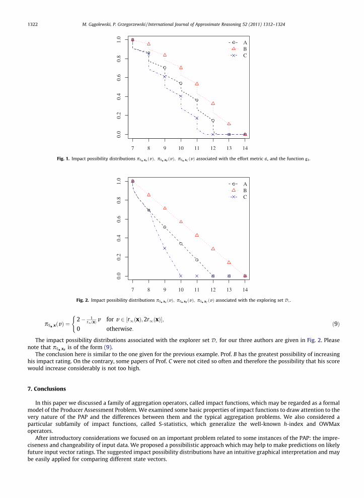
Fig. 1. Impact possibility distributions pSN ;xAðvÞ; pSN ;xB ðvÞ; pSN ;xC ðvÞ associated with the effort metric d⁄ and the function g1.

Fig. 2. Impact possibility distributions pSN ;xAðvÞ; pSN ;xB ðvÞ; pSN ;xC ðvÞ associated with the exploring set D� .


pSN ;xðvÞ ¼2� 1

r1ðxÞv for v 2 ½r1ðxÞ;2r1ðxÞ�;0 otherwise:

(ð9Þ

The impact possibility distributions associated with the explorer set D� for our three authors are given in Fig. 2. Pleasenote that pSN ;xB is of the form (9).

The conclusion here is similar to the one given for the previous example. Prof. B has the greatest possibility of increasinghis impact rating. On the contrary, some papers of Prof. C were not cited so often and therefore the possibility that his scorewould increase considerably is not too high.

7. Conclusions

In this paper we discussed a family of aggregation operators, called impact functions, which may be regarded as a formalmodel of the Producer Assessment Problem. We examined some basic properties of impact functions to draw attention to thevery nature of the PAP and the differences between them and the typical aggregation problems. We also considered aparticular subfamily of impact functions, called S-statistics, which generalize the well-known h-index and OWMaxoperators.

After introductory considerations we focused on an important problem related to some instances of the PAP: the impre-ciseness and changeability of input data. We proposed a possibilistic approach which may help to make predictions on likelyfuture input vector ratings. The suggested impact possibility distributions have an intuitive graphical interpretation and maybe easily applied for comparing different state vectors.


All tools proposed in this paper may support the decision process and hence be useful in many areas, e.g. in scientomet-rics, marketing, management, etc. The proposed impact possibility distributions may for example be recommended as acomplement to the Hirsch index.

However, many questions related to impact functions and the proposed prediction methods are still open. For example,the prediction based on the effort metrics may take into account different weights attributed to particular products, e.g.when it is much easier to increase the rating of a ‘‘good’’ product than of the ‘‘worse’’ one or when the costs required forgetting a new product seem to be higher than those needed for the improvement of an existing one.

On the other hand, the prediction based on the exploring sets enables a precise requirement specification for each stage ofthe improvement process. It might be of special interest if the impact function under study takes a countable number of val-ues only.

Of course, the choice of appropriate exploring sets or effort metrics is always dependent on the context or application ofconcern. However, some more formal, property-based approach to the topic deserves consideration in further research.

Moreover, we still lack some general S-statistics coefficient triangles construction methods. For related work on OWA andsimilar operators compare, e.g. [26,39,27,40].

Acknowledgments

The authors would like to express their gratitude to the Editor and the anonymous referees for their careful attention andprecious suggestions to improve the manuscript.

References

[1] M. Grabisch, E. Pap, J.-L. Marichal, R. Mesiar, Aggregation Functions, Cambridge, 2009.[2] J.E. Hirsch, An index to quantify individual’s scientific research output, PNAS 102 (46) (2005) 16569–16572.[3] M. Gagolewski, P. Grzegorzewski, S-statistics and their basic properties, in: C. Borgelt et al. (Eds.), Combining Soft Computing and Statistical Methods

in Data Analysis, Springer-Verlag, 2010, pp. 281–288.[4] M. Gagolewski, P. Grzegorzewski, Arity-monotonic extended aggregation operators, CCIS 80 (2010) 693–702.[5] G. Mayor, T. Calvo, On extended aggregation functions, Proc. IFSA 1997, vol. 1, Academia, Prague, 1997, pp. 281–285.[6] T. Calvo, A. Kolesarova, M. Komornikova, R. Mesiar, Aggregation operators: properties, classes and construction methods, in: T. Calvo, G. Mayor, R.

Mesiar (Eds.), Aggregation Operators. New Trends and Applications, Studies in Fuzziness and Soft Computing, vol. 97, Physica-Verlag, New York, 2002,pp. 3–104.

[7] R.R. Yager, On generalized Bonferroni mean operators for multi-criteria aggregation, International Journal of Approximate Reasoning 50 (2009) 1279–1286.

[8] R.R. Yager, On ordered weighted averaging aggregation operators in multictriteria decision making, IEEE Transactions on Systems, Man, andCybernetics 18 (1) (1988) 183–190.

[9] D. Dubois, H. Prade, C. Testemale, Weighted fuzzy pattern matching, Fuzzy Sets and Systems 28 (1988) 313–331.[10] D. Dubois, H. Prade, Formal representations of uncertainty, in: D. Bouyssou, D. Dubois, M. Pirlot, H. Prade (Eds.), Decision-Making Process, ISTE, London,

UK, 2009 (Chapter 3).[11] G.J. Klir, B. Yuan, Fuzzy Sets and Fuzzy Logic. Theory and Applications, Prentice-Hall, PTR, New Jersey, 1995.[12] S. Destercke, D. Dubois, E. Chojnacki, Unifying practical uncertainty representations. I: Generalized p-boxes, International Journal of Approximate

Reasoning 49 (3) (2008) 649–664.[13] S. Destercke, D. Dubois, E. Chojnacki, Unifying practical uncertainty representations. II: Clouds, International Journal of Approximate Reasoning 49 (3)

(2008) 664–677.[14] D. Dubois, H. Prade, P. Smets, A definition of subjective possibility, International Journal of Approximate Reasoning 48 (2) (2008) 352–364.[15] G.J. Woeginger, An axiomatic analysis of Egghe’s g-index, Journal of Informetrics 2 (4) (2008) 364–368.[16] G.J. Woeginger, An axiomatic characterization of the Hirsch-index, Mathematical Social Sciences 56 (2) (2008) 224–232.[17] T. Marchant, An axiomatic characterization of the ranking based on the h-index and some other bibliometric rankings of authors, Scientometrics 80 (2)

(2009) 325–342.[18] T. Marchant, Score-based bibliometric rankings of authors, Journal of the American Society for Information Science and Technology 60 (6) (2009)

1132–1137.[19] I. Palacios-Huerta, O. Volij, The measurement of intellectual influence, Econometrica 72 (3) (2004) 963–977.[20] A. Quesada, More axiomatics for the Hirsch index, Scientometrics 82 (2010) 413–418.[21] B. de Finetti, Sul significato soggettivo della probabilitá, Fundamenta Mathematicae 17 (1931) 298–329.[22] J. von Neumann, O. Morgenstern, Theory of Games and Economic Behavior, Princeton University Press, Princeton, 1947.[23] K.J. Arrow, A difficulty in the concept of social welfare, Journal of Political Economy 58 (4) (1950) 328–346.[24] K.O. May, A set of independent necessary and sufficient conditions for simple majority decision, Econometrica 20 (4) (1952) 680–684.[25] T. Calvo, G. Mayor, Remarks on two types of extended aggregation functions, Tatra Mountains Mathematical Publications 16 (1999) 235–253.[26] B.S. Ahn, Parameterized OWA operator weights: an extreme point approach, International Journal of Approximate Reasoning 51 (7) (2010) 820–831.[27] T. Calvo, G. Mayor, J. Torrens, J. Suner, M. Mas, M. Carbonell, Generation of weighting triangles associated with aggregation functions, International

Journal of Uncertainty, Fuzziness and Knowledge-based Systems 8 (4) (2000) 417–451.[28] P. Ball, Index aims for fair ranking of scientists, Nature 436 (2005) 900.[29] S. Alonso, F.J. Cabrerizo, E. Herrera-Viedma, F. Herrera, h-index: a review focused on its variants, computation and standardization for different

scientific fields, Journal of Informetrics 3 (2009) 273–289.[30] Y. Benjamini, Y. Hochberg, Controlling false discovery rate: a practical and powerful approach to multiple testing, Journal of the Royal Statistical

Society. Series B 57 (1) (1995) 289–300.[31] V. Torra, Y. Narukawa, The h-index and the number of citations: two fuzzy integrals, IEEE Transactions on Fuzzy Systems 16 (3) (2008) 795–797.[32] M. Franceschet, A comparison of bibliometric indicators for computer science scholars and journals on Web of Science and Google Scholar,

Scientometrics 83 (1) (2010) 243–258.[33] E.S. Vieira, J.A.N.F. Gomes, A comparison of Scopus and Web of Science for a typical university, Scientometrics 81 (2) (2009) 587–600.[34] E. Garfield, Can citation indexing be automated? in: M.E. Stevens, V.E. Giuliano, L.B. Heilprin (Eds.), Proceedings of the Statistical Association Methods

for Mechanized Documentation, Washington, 1964, pp. 189–192.[35] L. Bornmann, H.-D. Daniel, What do citation counts measure? A review of studies on citing behavior, Journal of Documentation 64 (1) (2008) 45–80.[36] P.M. Davis, Reward or persuation? The battle to define the meaning of a citation, Learned Publishing 21 (2009) 5–11.


[37] M. Gagolewski, P. Grzegorzewski, A geometric approach to the construction of scientific impact indices, Scientometrics 81 (3) (2009) 617–634.[38] M. Gagolewski, P. Grzegorzewski, Possible and necessary h-indices, in: Proceedings of the IFSA/Eusflat, 2009, pp. 1691–1695.[39] B.S. Ahn, Preference relation approach for obtaining OWA operators weights, International Journal of Approximate Reasoning 47 (2) (2008) 166–178.[40] R.R. Yager, Prioritized aggregation operators, International Journal of Approximate Reasoning 48 (1) (2008) 263–274.

possibilistic analysis of arity-monotonic aggregation operators and its relation to bibliometric...

Documents