positioning in wireless communications systems (sand/positioning in wireless communications systems)...
TRANSCRIPT

4Position Estimation
In this chapter, we address how to calculate the MT position, given a set of measurements
according to Chapter 3 in a static scenario, using the position principles presented in Chapter 2.
We assume that the MT is stationary during the position estimation process. Thus, the MT
position is deterministic. In Chapter 5, we extend the static position estimation to the dynamic
position tracking.
In this chapter, we consider ideal and erroneous measurements. With erroneous measure-
ments, we mean measurements that are noisy or biased, for example, due to thermal noise or
unknown MT clock offset for TOA measurements. However, we do not consider in this chapter
measurement errors due to multipath and NLOS propagation. For that, we refer the reader
to Chapter 7.
In the following section, we present the navigation equations for the positioning principles in
Chapter 2. To allow a simple visualization, we restrict ourselves to a two-dimensional planar
space. By default, we assume Cartesian coordinates. Where appropriate, we will extend our
considerations to three-dimensional space.
The BSs are located at
xi =(xi yi
)T, i = 1, … ,N
and the MT is located at
x =(x y
)T.
The distance between i-th BS and the MT is given by
di = di(x) = ||x − xi||2 =√
(x − xi)2 + (y − yi)2.
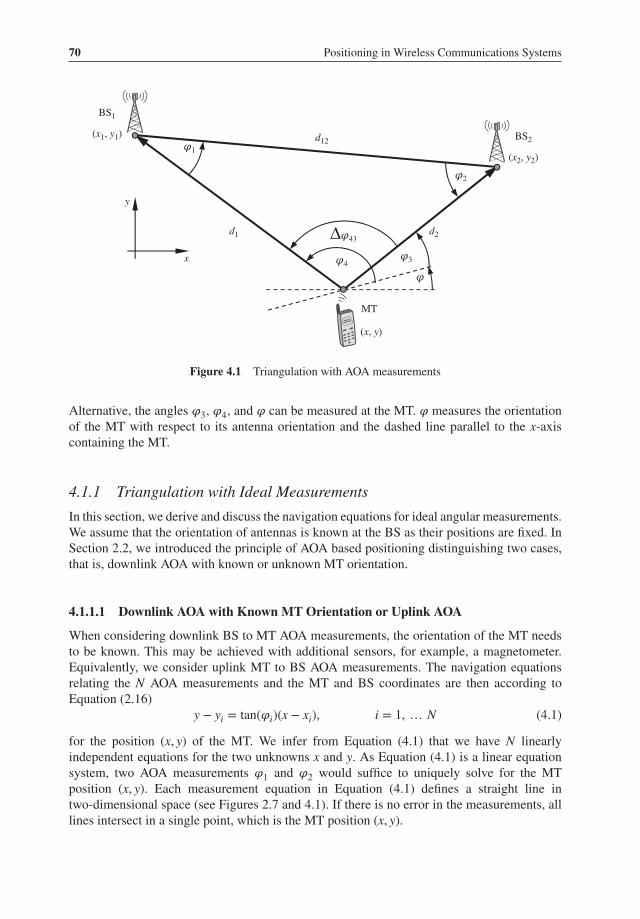
4.1 Triangulation
In triangulation, the MT and two BSs form a triangle, where the length and orientation of
the base line d12 between the two BSs is known and the AOAs 𝜑1 = ∠BS2BS1MT and 𝜑2 =∠MTBS2BS1 are measured in uplink transmissions from the MT to the BSs (see Figure 4.1).
Positioning in Wireless Communications Systems, First Edition. Stephan Sand, Armin Dammann and Christian Mensing.© 2014 John Wiley & Sons, Ltd. Published 2014 by John Wiley & Sons, Ltd.
70 Positioning in Wireless Communications Systems
d12𝜑1
𝜑2
MT
x
y
BS1
(x1, y1) BS2
(x2, y2)
(x, y)
d1 d2Δ𝜑43
𝜑3𝜑4
𝜑
Figure 4.1 Triangulation with AOA measurements
Alternative, the angles 𝜑3, 𝜑4, and 𝜑 can be measured at the MT. 𝜑 measures the orientationof the MT with respect to its antenna orientation and the dashed line parallel to the x-axiscontaining the MT.
4.1.1 Triangulation with Ideal Measurements
In this section, we derive and discuss the navigation equations for ideal angular measurements.We assume that the orientation of antennas is known at the BS as their positions are fixed. InSection 2.2, we introduced the principle of AOA based positioning distinguishing two cases,that is, downlink AOA with known or unknown MT orientation.
4.1.1.1 Downlink AOA with Known MT Orientation or Uplink AOA
When considering downlink BS to MT AOA measurements, the orientation of the MT needsto be known. This may be achieved with additional sensors, for example, a magnetometer.Equivalently, we consider uplink MT to BS AOA measurements. The navigation equationsrelating the N AOA measurements and the MT and BS coordinates are then according toEquation (2.16)
y − yi = tan(𝜑i)(x − xi), i = 1, … N (4.1)
for the position (x, y) of the MT. We infer from Equation (4.1) that we have N linearlyindependent equations for the two unknowns x and y. As Equation (4.1) is a linear equationsystem, two AOA measurements 𝜑1 and 𝜑2 would suffice to uniquely solve for the MTposition (x, y). Each measurement equation in Equation (4.1) defines a straight line intwo-dimensional space (see Figures 2.7 and 4.1). If there is no error in the measurements, alllines intersect in a single point, which is the MT position (x, y).

Position Estimation 71
Analytical Solution to Triangulation EquationsTo solve Equation (4.1), the BSs measure the AOAs 𝜑1 and 𝜑2 in Figure 4.1 (see Section 3.3).
Further, the coordinates (x1, y1) and (x2, y2) of the two BSs need to be known. Then, we can
relate the MT coordinates with the measured angles and the BS coordinates as
tan𝜑1 =y − y1
x − x1
and tan𝜑2 =y − y2
x − x2
.
Solving this equation for y, we obtain
y = (tan𝜑1)x + y1 − tan𝜑1x1 = a1x + b1,
y = (tan𝜑2)x + y2 − tan𝜑2x2 = a2x + b2. (4.2)
These two equations represent two lines, whose intersection point (x, y) is the MT position.
Solving Equation (4.2) for the constants b1 and b2, and using vector-matrix notation, we obtain(−a1 1
−a2 1
)(xy
)=(
b1
b2
). (4.3)
To solve the linear equation system (4.3), we simply invert the 2 × 2 matrix(xy
)=(−a1 1
−a2 1
)−1(b1
b2
)= 1
a2 − a1
(1 a2
−1 −a1
)(b1
b2
)= 1
tan𝜑2 − tan𝜑1
(y1 − tan𝜑1x1 + tan𝜑2
(y2 − tan𝜑2x2
)−y1 + tan𝜑1x1 − tan𝜑1(y2 − tan𝜑2x2)
). (4.4)
Note that Equation (4.4) only holds if a1 = tan𝜑1 ≠ a2 = tan𝜑2, that is, the two AOAs are
not measured from exactly the same or opposite direction.
4.1.1.2 Downlink AOA with Unknown MT Orientation
In general, the orientation 𝜑 of the MT is unknown when using downlink AOA measurements
(see Figure 4.1). Thus, it becomes an additional parameter that needs to be estimated to obtain
the MT position (x, y). Therefore, Equation (4.1) becomes
y − yi = tan(𝜑i + 𝜑)(x − xi), i = 1, … N. (4.5)
As explained in Section 2.2.1, Equation (4.5) is nonlinear in 𝜑. When 𝜑 is unknown and we
have only two AOA measurements 𝜑1 and 𝜑2, the location of the MT is limited to an arc
of a circle inscribing a triangle defined with baseline d =√(x1 − x2)2 + (y1 − y2)2 and angle
𝜑2 − 𝜑1 opposite the baseline d. Thus, at least three AOA measurements are needed to esti-
mate the MT position uniquely in contrast to Equation (4.1). Alternative, we can rearrange
Equation (4.5) so it is linear with respect to the angles 𝜑i and 𝜑, but nonlinear with respect to
the coordinates x and y:
arctan
(y − yi
x − xi
)= 𝜑i + 𝜑, i = 1, … N. (4.6)

72 Positioning in Wireless Communications Systems
Thus, the unknown MT orientation in Equation (4.6) is similar to the unknown clockbias b between the MT and BSs for TOA measurements (see Section 2.1.1.2). For TOAmeasurements, we computed the difference between a reference TOA and the other TOAmeasurements to remove the unknown clock bias b. This resulted in TDOA based positioning(see Section 2.1.2). Thus, we can subtract Equation (4.6) for i = 1 from Equation (4.6) fori = 2, … ,N to obtain
Δ𝜑i1 = arctan
(y − yi
x − xi
)− arctan
(y − y1
x − x1
), i = 2, … N. (4.7)
Here, Δ𝜑i1 = 𝜑i − 𝜑1 denotes the AOA difference (AOAD) measurements.In the following, we present an alternative approach for AOA positioning with unknown MT
orientation 𝜑. For that, we use the law of cosines, that is,
c2 = a2 + b2 − 2ab cosΔ𝜑,
to obtain the set of nonlinear equations
d21i = d2
1+ d2
i − 2d1di cos(𝜑i − 𝜑1)
(x1 − xi)2 + (y1 − yi)2 = (x − x1)2 + (y − y1)2 + (x − xi)2 + (y − yi)2
− 2
√(x − x1)2 + (y − y1)2
√(x − xi)2 + (y − yi)2 ⋅ cos (𝜑i − 𝜑1)
⏟⏞⏞⏟⏞⏞⏟=∶Δ𝜑i1
,
i = 2, … ,N. (4.8)
The cosines in Equation (4.8) are calculated for AOAD measurements Δ𝜑i1 = 𝜑i − 𝜑1 fromthe AOA measurements 𝜑i, i = 2, … ,N and the arbitrarily chosen AOA reference measure-ment 𝜑1. In Figure 4.1, we used 𝜑3 as reference measurement. Thus, the orientation 𝜑 of theMT is removed compared to Equation (4.5) and only N − 1 equations remain. This is similarto TDOA based positioning, when the unknown clock bias b between the MT and the BS forTOA measurements is removed by computing the difference between a reference TOA andthe other TOA measurements (see Section 2.1.2). Similar to Equations (4.5) and (4.6), we cansolve Equation (4.8) for Δ𝜑i1
Δ𝜑i1 =
arccos
((x − x1
)2 + (y − y1)2 + (x − xi)2 + (y − yi)2 − (x1 − xi)2 − (y1 − yi)2
2√(x − x1)2 + (y − y1)2
√(x − xi)2 + (y − yi)2
)i = 2, … ,N. (4.9)
The benefits of Equations (4.6), (4.7), and (4.9) will be explained in Section 4.1.2.We can obtain a polynomial equation system with respect to the unknowns x and y from
Equation (4.8) by solving for the square root terms and squaring each equation, that is,
4((
x − x1
)2 + (y − y1)2)((
x − xi
)2 + (y − yi)2)⋅ cos2(Δ𝜑i1) =((
x − x1
)2 + (y − y1)2 + (x − xi)2 + (y − yi)2 − (x1 − xi)2 − (y1 − yi)2)2
,
i = 2, … ,N. (4.10)

Position Estimation 73
Comparing Equation (4.10) with Equations (4.7) or (4.9), we note that the first equation sys-
tem is polynomial in x and y whereas the later ones are transcendental. Thus, the navigation
equation (4.10) promises a lower complexity and possibly a more numerically stable solu-
tion than Equation (4.7). Nevertheless, Equations (4.7) and (4.9) are beneficial for erroneous
measurements (see Section 4.1.2).
Given three independent AOA measurements from three different BSs, we obtain two inde-
pendent polynomial equations with maximum degree of four for both x and y according to
Equation (4.10). As two circles intersect at most at two places the resulting four circles inter-
sect at most at 12 places.
Example 4.1.1 (AOAD solution geometry) Here, BS1 is located at (x, y) = (0 m, 0 m), BS2
at (100 m, 0 m), and BS3 at (0 m, 100 m). The MT measured the AOADs Δ𝜑21 = 150∘ andΔ𝜑31 = −75∘. The solution geometry defined by Equation (4.10) is plotted in Figure 4.2. Asexplained, the two polynomial equations with a maximum degree of 4 in Equation (4.10) resultin two pairs of circles (one small and one large pair) that intersect at 12 points. The intersec-tion points 1, 2, 3, 4,BS2, and BS3 have a multiplicity of one and the intersection point BS1
a multiplicity of six. Due to the squaring to obtain Equation (4.10), any of the intersectionpoints between the pair of small and large circles, that is, 1, 2, 3, 4, and BS1, could be a pos-sible position of the MT. However, assuming a non-zero distance to BS1 and given the AOADmeasurements Δ𝜑21 = 150∘ and Δ𝜑31 = −75∘, only point 4 is the valid position solution.
1
23
4MT
BS2BS1
BS3
200
150
100
50
−50
−100
−150
−200−200 −150 −100 −50 0
x [m]
50 100 150 200
0
y [m
]
Figure 4.2 AOAD measurements from three BSs and solution geometry according to Equation (4.10)
74 Positioning in Wireless Communications Systems
Numerical Solution to Triangulation with Unknown MT OrientationIn this case, we have to solve one of the nonlinear Equations (4.5)–(4.10). To the best of
our knowledge, only the Equations (4.8) and (4.10) might have rather complex closed form
solutions. Nevertheless, we will present here two iterative algorithms, the Newton–Raphson
and Gauss–Newton algorithms (Kay 1993; Press et al. 1992), to solve the nonlinear navigation
equations of Section 4.1 adapted to the nonlinear least squares problem. Apart from these two
algorithms, other algorithms such as steepest descent or Levenberg–Marquardt exist to solve
the nonlinear navigation equations (see Sections 4.2.2.3 and 4.3.2.1).
Newton–Raphson algorithm. Given the previous equations for unknown MT orientation, we
could try to directly solve the nonlinear equations, that is,
f (𝜽) =(f1 (𝜽) · · · fN(𝜽)
)T, (4.11)
where fi(𝜽) = 0 corresponds to the i-th element in Equations (4.5)–(4.10), for example,
fi(𝜽) = fi((x, 𝜑)T) = y − yi − tan(𝜑i + 𝜑)(x − xi) = 0 for Equation (4.5). Note that for
Equations (4.7) or (4.8)–(4.10) we have, instead of N, only N − 1 equations. Nevertheless,
the following derivations and equations also hold for Equations (4.7)–(4.10) assuming that
we have reduced the dimensions of vectors and matrices accordingly. The vector 𝜃 ∈ ℝM
contains the M unknowns, for example, x, y, and 𝜑 for Equation (4.5). Instead of directly
computing the solution to Equation (4.11), it is numerically more stable to minimize the
quadratic cost function (Press et al. 1992)
C(𝜽) = 1
2fT (𝜽) f (𝜽) = 1
2
N∑i= 0
f 2i (𝜽). (4.12)
Note that C(𝜽) defines the nonlinear least squares problem (Kay 1993). Next, we compute the
gradient of C(𝜽) and set it equal to zero to minimize Equation (4.12):
g(𝜽) = ∇𝜽C(𝜽) =N∑
i= 0
∇𝜽 fi(𝜽) fi(𝜽) = (∇𝜽 ⊗ fT (𝜽))⏟⏞⏞⏞⏞⏞⏞⏟⏞⏞⏞⏞⏞⏞⏟
=∶𝚽T (𝜽)
f (𝜽) = 𝚽T (𝜽) f (𝜽)!= 𝟎M , (4.13)
where ∇𝜽 =(
𝜕
𝜕𝜃1, … 𝜕
𝜕𝜃M
)T
, ⊗ denotes the Kronecker product, and 𝚽(𝜽) the N × M
Jacobian matrix. Note, Equation (4.13) is a system of M simultaneous nonlinear equations
with respect to 𝜽. To solve these equations, we apply the Newton–Raphson method (Kay
1993) to the function g(𝜽) in Equation (4.13). Then, the k-th iteration is given by
𝜽(k+1) = 𝜽(k) −((Γ (𝜽))−1g(𝜽)
)|||𝜽=𝜽(k) , (4.14)
with the M × M Jacobian matrix
Γ(𝜽) = ∇T
𝜽⊗ g(𝜽) = ∇T
𝜽⊗ ((∇𝜽 ⊗ fT (𝜽))f (𝜽))
= 𝚽T (𝜽)𝚽 (𝜽) +N∑
i=1
fi(𝜽)Hfi(𝜽)(4.15)

Position Estimation 75
and the M × M Hessian matrix
Hfi(𝜽)= (∇𝜽 ⊗ ∇T
𝜽)fi(𝜽) =
⎛⎜⎜⎜⎜⎜⎜⎝
𝜕2fi(𝜽)𝜕𝜃2
1
𝜕2fi(𝜽)𝜕𝜃1𝜕𝜃2
· · · 𝜕2fi(𝜽)𝜕𝜃1𝜕𝜃M
𝜕2fi(𝜽)𝜕𝜃2𝜕𝜃1
𝜕2fi(𝜽)𝜕𝜃2
2
· · · 𝜕2fi(𝜽)𝜕𝜃2𝜕𝜃M
⋮ ⋱ ⋱ ⋮𝜕2fi(𝜽)𝜕𝜃M𝜕𝜃1
· · · 𝜕2fi(𝜽)𝜕𝜃M𝜕𝜃M−1
𝜕2fi(𝜽)𝜕𝜃2
M
⎞⎟⎟⎟⎟⎟⎟⎠. (4.16)
Example 4.1.2 (Newton–Raphson iteration for triangulation with AOAD) In the fol-lowing, we apply the Newton–Raphson iterations (see Equations 4.14–4.16) to the AOADEquation (4.10) and the parameters of Example 4.1.1. Thus, the parameter vector only con-tains the x- and y-coordinates of the MT, that is, 𝜽 = (x, y)T. The function f (𝜽) then becomes
f (𝜽) = 4
((x2 + y2 − xx2
)2 − cos2(Δ𝜑21
) (x2 + y2
) (x2 + y2 − 2xx2 + x2
2
)(x2 + y2 − yy3
)2 − cos2(Δ𝜑31
) (x2 + y2
) (x2 + y2 − 2yy3 + y2
3
)) ,
with x2 = y3 = 100 m, Δ𝜑21 = 150∘, and Δ𝜑31 = −75∘. Thus, given f (𝜽) in the previousequation, we can compute a Newton–Raphson iteration by calculating
1. g(𝜽) in Equation (4.13),2. Γ(𝜽) in Equation (4.15), and3. finally, evaluating Equation (4.14) at 𝜽 = 𝜽(k) to obtain the estimate 𝜽(k+1).
We start this algorithm with an initial value of 𝜽(0). Then, we repeat the three steps until anew update changes less than a predefined tolerance 𝜖TOL, that is,||||||𝜽(k+1) − 𝜽(k)
||||||2 < 𝜖TOL.
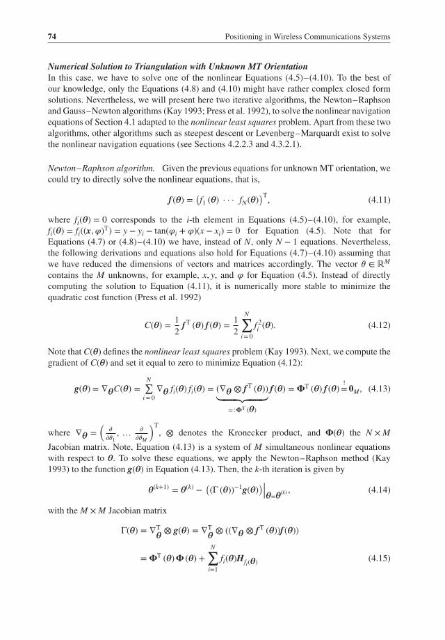
Figure 4.3 shows the scenario including the Newton–Raphson iterations (+ markers). Weinitialize the algorithm with the starting point (100 m, 100 m). The algorithm converges tothe correct MT position at (50 m, 13.4 m) after 11 iterations. Note that the algorithm is verysensitive to the starting point. For instance, it converges to the point (16.14 m, 7.5 m) if wechose the mean position of the measured BSs, that is, x̂(0) = 1∕N
∑Ni=1 xi = (33.3 m, 33.3 m)T.
This point is a valid solution to Equation (4.10). However, if we check the estimated solutionwith the measured AOADs, we see that Δ𝜑31 = 105∘ instead of the correct 75∘. Thus, theposition estimation could chose another starting point until the position solution yields thecorrect AOADs.
Gauss–Newton Algorithm. Instead of directly working with the nonlinear function f (𝜽), wenow linearize Equation (4.11) at 𝜽(k):
f (𝜽) ≈ f̃ (𝜽) = f(𝜽(k))+ 𝚽 (𝜽)|
𝜽=𝜽(k)(𝜽 − 𝜽(k)
). (4.17)
Thus the N × M Jacobian matrix of the linearized function f̃ (𝜽) is
�̃�(𝜽) = ∇T
𝜽⊗ f̃ (𝜽) = 𝚽 (𝜽)|
𝜽=𝜽(k) . (4.18)
76 Positioning in Wireless Communications Systems
MTBS2BS1
BS3
Newton–Raphsoniterations
200
150
100
50
−50
−100
−150
−200−200 −150 −100 −50 0
x [m]
50 100 150 200
0
y [m
]
Figure 4.3 Solution to the navigation equation for AOAD measurements from three BSs with
Newton–Raphson method: Pluses indicate the Newton–Raphson iterations starting at (100 m, 100 m).Convergence is achieved after 11 iterations
Consequently, the function
g̃(𝜽) = 𝚽T (𝜽)|||𝜽=𝜽(k)
(f(𝜽(k))+ 𝚽 (𝜽)|
𝜽=𝜽(k)(𝜽 − 𝜽(k)
))(4.19)
is now linear in 𝜽. Hence, setting g̃(𝜽)!= 0 and solving for 𝜽 yields the Gauss–Newton iteration
𝜽(k+1) = 𝜽(k) −((
𝚽T (𝜽)𝚽(𝜽))−1𝚽T (𝜽)
)||||𝜽=𝜽(k)f(𝜽(k)). (4.20)
4.1.1.3 Extension to Three Dimensions
In the remainder of this section, we extend these considerations to three-dimensional naviga-
tion (see Section 2.2.2). Figure 2.9 depicts the three-dimensional setup. In three-dimensional
space, we can measure, in addition to the two azimuth angles 𝜑1 and 𝜑2, two elevation angles
𝜗1 and 𝜗2. The relations between the x- and y-coordinates in Equation (4.5) still hold in
three-dimensional space. Thus, we can obtain from Section 2.2.2 and Figure 2.9 the following
relations for the azimuth and elevation angles:(y − yi
)= tan
(𝜑i + 𝜑
) (x − xi
),
cos(𝜑i + 𝜑
) (z − zi
)= tan
(𝜗i + 𝜗
) (x − xi
), i = 1, … ,N,
(4.21)
Position Estimation 77
or with di,𝟐D =√(x − xi)2 + (y − yi)2 for the second line in Equation (4.21)(
z − zi
)= tan
(𝜗i + 𝜗
)di,2D, i = 1, … ,N. (4.22)
In Equation (4.21), we have the five unknowns x, y, z, 𝜑, and 𝜗. Thus, at least five AOA
measurements are needed, for example, three azimuth and two elevation AOAs. Similar
to Equations (4.5), (4.6), and (4.7), we formulate the modified navigation equations for
Equation (4.21) as
arctan
(y − yi
x − xi
)= 𝜑i + 𝜑,
arctan
(z − zi
di,2D
)= 𝜗i + 𝜗, i = 1, … ,N.
(4.23)
and as
arctan
(y − yi
x − xi
)− arctan
(y − y1
x − x1
)= Δ𝜑i1
arctan
(z − zi
di,2D
)− arctan
(z − z1
d1,2D
)= Δ𝜗i1 i = 2, … ,N.
(4.24)
Besides Equations (4.23) and (4.24), we can alternatively compute the z-coordinate of the
MT position according to Figure 4.4 and the law of cosines as
a2i =(x − xi
)2 +(y − yi
)2 +(z − zi
)2,
b2i =(x − x1
)2 +(y − y1
)2 +(z − z1
)2,
c2i =(√(
x − xi
)2 +(y − yi
)2 −√(
x − x1
)2 +(y − y1
)2)2
+(zi − z1
)2,
= a2i + b2
i − 2aibi cos(Δ𝜗i1
), i = 2, … ,N,
(4.25)
or
Δ𝜗i1 = arccos
(a2
i + b2i − c2
i
2aibi
), i = 2, … ,N, (4.26)
where Δ𝜗i1 = 𝜗i − 𝜗1 is the elevation AOAD. Thus, we can obtain the z-coordinate of the MT
position with one AOAD measurement from Equation (4.25), which is an algebraic equation
in z. By squaring the last line of Equation (4.25), we obtain a fourth order polynomial equation
in z, that is, a quartic equation, which can be solved analytically.
As the relations between the azimuth angles and the x- and y-coordinates are independent of
the z-coordinate, we can compute the position of the MT in two steps:
1. We compute the Cartesian coordinates of the MT in the xy-plane according to Equation (4.1)
for known 𝜑 or according to Equations (4.5)–(4.10) for unknown 𝜑.
2. We compute the z-coordinate of the MT according to one of the Equations (4.21)–(4.26)
given the estimates for x, y, and possibly 𝜑, and at least one elevation AOA 𝜗i for known 𝜗,
or two elevation AOAs for unknown 𝜗.

78 Positioning in Wireless Communications Systems
rxy
(x, y)
(x–x1)2 + (y–y1)2
zi –z1
(x–xi)2 + (y–yi)
2
� x2
i + y2i, zi
�
� x2
1 + y21 , z1
�
MT
z
BS1
BSi
b
ca
𝜗1 + 𝜗
𝜗i + 𝜗
Δ𝜗i1
Figure 4.4 Step 2 of 3D AOA estimation with AOAD Δ𝜗i1
Note that for computing the three-dimensional position of the MT, we only need to measurethree angles, for example, the two azimuth angles 𝜑1 and 𝜑2 as well as the elevation angle 𝜗1
if the MT orientation is known. From Figure 2.9, we may geometrically interpret this as fol-lows: When computing the x- and y-coordinates of the MT first, the three-dimensional positionsolution to the MT lies on the intersection of two planes. These planes are perpendicular to thexy-plane and contain the points (x1, y1) and (x, y) or (x2, y2) and (x, y). The intersection of thetwo planes forms a line parallel to the z-coordinate, on which the MT lies. Given one elevationangle as third measurement, we uniquely determine the MT position (x, y, z). However, we needto measure at least five angles if the MT orientation is unknown, that is, 𝜑1, 𝜑2, 𝜑3, 𝜗1, and 𝜗2.
Analytical Solution to the Triangulation Equations with Known MT OrientationThe previous calculations show that it is sufficient to just have two azimuth angle measure-ments for planar navigation if the MT orientation is known or uplink AOAs are measured at theBSs. In the case of three-dimensional navigation, three angular measurements, for example,two azimuth angles and one elevation angle, are necessary to compute the MT position. Thus,the z-coordinate of the MT position is calculated from Equation (4.21) as
z = z1 + tan(𝜗1)d1,2D,
where d1,2D =√(x − x1)2 + (y − y1)2 can be calculated given the solution from Equation (4.4).
Numerical Solution to the Triangulation Equations with Unknown MT OrientationIn this case, we have to solve one of the nonlinear Equations (4.21)–(4.26). To the best ofour knowledge, only Equation (4.25) might have a rather complex closed form solutions.
Position Estimation 79
In Section 4.1.1.2, we presented the Newton–Raphson and Gauss–Newton algorithmfor the two-dimensional Equations (4.5)–(4.10). The extension to the three-dimensionalEquations (4.21)–(4.26) is straightforward. We simply have to modify f (𝜽) in Equation (4.11)and then, subsequently in Equations (4.12)–(4.20).
4.1.2 Triangulation with Erroneous Measurements
In contrast to the previous section, any practical system cannot provide ideal measurements.The measurements are erroneous due to various effects, such as thermal noise in the electriccircuits, limited angular resolution of the measurement equipment, uncertainties in the BSpositions, and so on. A common assumption is that the AOA measurement errors are disturbedby AWGN (see Section 3.3.2, Figueiras and Frattasi 2010; Zekavat and Buehrer 2012):
�̂�i = 𝜑i + 𝜑𝜖i, 𝜑𝜖i
∼ (0, 𝜎2
𝜑𝜖i
), i = 1, … ,N (4.27)
and
�̂�i = 𝜗i + 𝜗𝜖i, 𝜗𝜖i
∼ (0, 𝜎2
𝜗𝜖i
), i = 1, … ,N. (4.28)
Hence, the navigation equations for triangulation with erroneous measurements can be simplyobtained from the ones for ideal measurements through replacing 𝜑i with �̂�i and 𝜗i with �̂�i inEquations (4.1), (4.5)–(4.10) and (4.21)–(4.26). Note that the AWGN on the AOAs �̂�i and �̂�iin Equations (4.27) and (4.28) is transformed through the trigonometric functions cos and tan toa multiplicative, non-Gaussian noise in the triangulation equations, that is, in Equations (4.1),(4.5), (4.8), (4.10), (4.21), (4.22), and (4.25). This will complicate the derivation of positionsolution algorithms, especially, the ML algorithms. Thus, the triangulation equations definedby Equations (4.6), (4.7), (4.9), (4.23), (4.24), and (4.26) are more suitable for noisy AOAmeasurements.
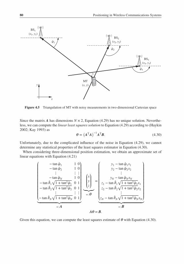
Figure 4.5 depicts a possible measurement scenario for two-dimensional navigation withnoisy measurements. Let us assume that N BS have measured the AOA of the MT receivedsignal, that is, �̂�i and �̂�i (i = 1, … ,N) according to Equation (4.27) and (4.28).
4.1.2.1 Linear Least Squares Solution to Erroneous AOA Measurements with KnownMT Orientation
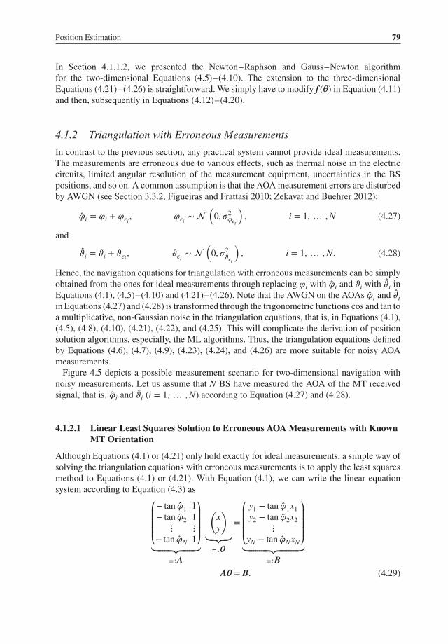
Although Equations (4.1) or (4.21) only hold exactly for ideal measurements, a simple way ofsolving the triangulation equations with erroneous measurements is to apply the least squaresmethod to Equations (4.1) or (4.21). With Equation (4.1), we can write the linear equationsystem according to Equation (4.3) as⎛⎜⎜⎜⎝
− tan �̂�1 1
− tan �̂�2 1
⋮ ⋮− tan �̂�N 1
⎞⎟⎟⎟⎠⏟⏞⏞⏞⏞⏞⏟⏞⏞⏞⏞⏞⏟
=∶A
(xy
)⏟⏟⏟=∶𝜽
=⎛⎜⎜⎜⎝
y1 − tan �̂�1x1
y2 − tan �̂�2x2
⋮yN − tan �̂�NxN
⎞⎟⎟⎟⎠⏟⏞⏞⏞⏞⏞⏞⏞⏞⏟⏞⏞⏞⏞⏞⏞⏞⏞⏟
=∶BA𝜽 = B. (4.29)
80 Positioning in Wireless Communications Systems
𝜑1ˆ
𝜑2ˆ
𝜑3ˆ
x
y
BS1
BS2
MT
(x1, y1)
(x2, y2)
BS3
(x3, y3)
(x, y)
Figure 4.5 Triangulation of MT with noisy measurements in two-dimensional Cartesian space
Since the matrix A has dimensions N × 2, Equation (4.29) has no unique solution. Neverthe-
less, we can compute the linear least squares solution to Equation (4.29) according to (Haykin
2002; Kay 1993) as
𝜽 =(ATA
)−1ATB. (4.30)
Unfortunately, due to the complicated influence of the noise in Equation (4.29), we cannot
determine any statistical properties of the least squares estimator in Equation (4.30).
When considering three-dimensional position estimation, we obtain an approximate set of
linear equations with Equation (4.21)
⎛⎜⎜⎜⎜⎜⎜⎜⎜⎜⎝
− tan �̂�1 1 0
− tan �̂�2 1 0
⋮ ⋮ ⋮− tan �̂�N 1 0
− tan �̂�1
√1 + tan2�̂�1 0 1
− tan �̂�2
√1 + tan2�̂�2 0 1
⋮ ⋮ ⋮− tan �̂�N
√1 + tan2�̂�N 0 1
⎞⎟⎟⎟⎟⎟⎟⎟⎟⎟⎠⏟⏞⏞⏞⏞⏞⏞⏞⏞⏞⏞⏞⏞⏞⏞⏞⏞⏞⏞⏞⏟⏞⏞⏞⏞⏞⏞⏞⏞⏞⏞⏞⏞⏞⏞⏞⏞⏞⏞⏞⏟
=∶A
⎛⎜⎜⎝xyz
⎞⎟⎟⎠⏟⏟⏟=∶𝜽
=
⎛⎜⎜⎜⎜⎜⎜⎜⎜⎜⎝
y1 − tan �̂�1x1
y2 − tan �̂�2x2
⋮yN − tan �̂�NxN
z1 − tan �̂�1
√1 + tan2�̂�1x1
z2 − tan �̂�2
√1 + tan2�̂�2x2
⋮zN − tan �̂�N
√1 + tan2�̂�NxN
⎞⎟⎟⎟⎟⎟⎟⎟⎟⎟⎠⏟⏞⏞⏞⏞⏞⏞⏞⏞⏞⏞⏞⏞⏞⏞⏞⏞⏞⏞⏞⏞⏟⏞⏞⏞⏞⏞⏞⏞⏞⏞⏞⏞⏞⏞⏞⏞⏞⏞⏞⏞⏞⏟
=∶BA𝜽 = B.
Given this equation, we can compute the least squares estimate of 𝜽 with Equation (4.30).

Position Estimation 81
4.1.2.2 Maximum Likelihood Solution to Erroneous Downlink AOA Measurementswith Unknown MT Orientation
In this section, we develop the ML position estimator for erroneous AOA measurements in
the downlink with unknown MT orientation. Similar to Section 4.1.1.2 we present the itera-
tive Newton–Raphson and Gauss–Newton algorithms to solve the weighted nonlinear leastsquares problem when the AOA measurements are corrupted by AWGN.
Given the navigation equation in Equation (4.6), we define the vector function
f (𝜽) =(f1 (𝜽) · · · fN(𝜽)
)T, (4.31)
where fi(𝜽) is given by
fi(𝜽) = arctan
(y − yi
x − xi
)− 𝜑, i = 1, … ,N.
The measurement vector is then
�̂� = f (𝜽) + 𝝋𝝐 =(f1 (𝜽) + 𝜑𝜖1
· · · fN(𝜽) + 𝜑𝜖N
)T,
with
𝝋𝝐 ∼ (𝟎N ,𝚺𝝋𝝐
)and 𝚺𝝋𝝐 = E
{𝝋𝝐𝝋
T𝝐
}.
If the AOA measurements are uncorrelated, 𝚺𝝋𝝐 ∈ ℝN × N becomes a diagonal matrix. For
the random vector �̂�, the log-likelihood function given f (𝜽) is
ln p ( �̂�| f (𝜽)) = −N2
ln (2𝜋) − 1
2ln det𝚺𝝋𝝐 − 1
2
((�̂� − f (𝜽)) T𝚺−1
𝝋𝝐(�̂� − f (𝜽))
).
Only the last term in the previous equation is a function of 𝜽. Thus, we define the ML cost
function as
L(𝜽) = −1
2(�̂� − f (𝜽)) T𝚺−1
𝝋𝝐(�̂� − f (𝜽)) . (4.32)
This cost function defines the weighted nonlinear least squares problem. To find the ML solu-
tion for Equation (4.32), we compute the gradient of L(𝜽) and equate it to the zero vector:
g(𝜽) = ∇𝜽L(𝜽) = ∇𝜽 ln p ( �̂�| f (𝜽))=
(∇𝜽 ⊗ fT (𝜽)
)𝚺−1𝝋𝝐
(�̂� − f (𝜽)) = 𝚽T (𝜽)𝚺−1𝝋𝝐
(�̂� − f (𝜽))!= 𝟎M . (4.33)
In the remainder of this subsection, we present the specifics for the iterative Newton–
Raphson and Gauss–Newton algorithms with respect to Equations (4.32) and (4.33).
Although, the derivations strictly hold only for the navigation equation defined by
Equation (4.6), it is very simple to modify the derivation so that we obtain the solutions for
Equations (4.7), (4.9), (4.23), (4.24), or (4.26).

82 Positioning in Wireless Communications Systems
Newton–Raphson AlgorithmAnalogously to Section 4.1.1.2, the Newton–Raphson iteration for the weighted nonlinearleast squares problem with erroneous AOA measurements in the downlink and unknown MTorientation is given by
𝜽(k+1) = 𝜽(k) −((Γ(𝜽)−1
)g(𝜽)
)|||𝜽=𝜽(k) ,
with the M × M Jacobian matrix
Γ(𝜽) = ∇T
𝜽⊗ g(𝜽) = ∇T
𝜽⊗
((∇𝜽 ⊗ fT (𝜽)
)𝚺−1𝝋𝝐
(�̂� − f (𝜽)))
=N∑
i=1
Hfi(𝜽)
(𝚺−1𝝋𝝐
(�̂� − f (𝜽)))
i−𝚽T (𝜽)𝚺−1
𝝋𝝐𝚽(𝜽),
where (⋅)i denotes the i-th element of a vector, and the M × M Hessian matrix
Hfi(𝜽)=
(∇𝜽 ⊗ ∇T
𝜽
)fi(𝜽) =
⎛⎜⎜⎜⎜⎜⎜⎝
𝜕2fi(𝜽)𝜕𝜃2
1
𝜕2fi(𝜽)𝜕𝜃1𝜕𝜃2
· · · 𝜕2fi(𝜽)𝜕𝜃1𝜕𝜃M
𝜕2fi(𝜽)𝜕𝜃2𝜕𝜃1
𝜕2fi(𝜽)𝜕𝜃2
2
· · · 𝜕2fi(𝜽)𝜕𝜃2𝜕𝜃M
⋮ ⋱ ⋱ ⋮𝜕2fi(𝜽)𝜕𝜃M𝜕𝜃1
· · · 𝜕2fi(𝜽)𝜕𝜃M𝜕𝜃M−1
𝜕2fi(𝜽)𝜕𝜃2
M
⎞⎟⎟⎟⎟⎟⎟⎠.
Gauss–Newton AlgorithmSimilar to Section 4.1.1.2, we now linearize Equation (4.31) at 𝜽(k):
f (𝜽) ≈ f̃ (𝜽) = f(𝜽(k)
)+ 𝚽 (𝜽)|
𝜽=𝜽(k)(𝜽 − 𝜽(k)
).
Thus, the N × M Jacobian matrix of the linearized function f̃ (𝜽) is
�̃�(𝜽) = ∇T
𝜽⊗ f̃ (𝜽) = 𝚽 (𝜽)|
𝜽=𝜽(k) .
Consequently, the function
g̃(𝜽) = 𝚽T (𝜽)|||𝜽=𝜽(k)𝚺−1𝝋𝝐
(�̂� − f
(𝜽(k)
)− 𝚽 (𝜽)|
𝜽=𝜽(k)(𝜽 − 𝜽(k)
))is now linear in 𝜽. Hence, setting g̃(𝜽)
!= 0 and solving for 𝜽 yields the Gauss–Newton iteration
𝜽(k+1) = 𝜽(k) +((
𝚽T (𝜽)𝚺−1𝝋𝝐
𝚽(𝜽))−1
𝚽T (𝜽))|||||𝜽=𝜽(k)
𝚺−1𝝋𝝐
(�̂� − f
(𝜽(k)
)).
4.2 Trilateration
In this section, we consider trilateration based on measured quantities whose values are afunction of the distance between the MT and BSs. Examples of such measurements are theTOA measurement (see Section 3.2) and the RSS (see Section 2.3.2).
For TOA, the relation between the distance the signal propagates and the time is
di = c(Ti − T0),
where c denotes the speed of light, Ti denotes the time instance at which the signal wasreceived, and T0 the time instance at which the signal was transmitted (see Section 2.1.1).

Position Estimation 83
For RSS, the relationship between the received signal power and the distance depends on thepropagation environment. Under ideal free space propagation conditions, the relationship is
di ∝
√Pt
Pr.
For more details, the reader may refer to Section 2.3.2.In the remainder of this section, we focus on trilateration with TOA measurements.
4.2.1 Trilateration with Ideal Measurements
For ideal TOA measurements, the navigation equation in two dimensions is given by (seeEquation 2.1)
di = c(Ti − T0) =√
(x − xi)2 + (y − yi)2, i = 1, … ,N. (4.34)
Squaring Equation (4.34), we obtain
d2i = (x − xi)2 + (y − yi)2 i = 1, … ,N, (4.35)
which defines N circles with center (xi, yi) and radius di. As shown in Figure 2.1, two circlesdefined by the TOA measurements intersect in two points, for example, BS1 and BS2. Onlywith a third circle defined by another TOA measurement, for example, BS3, the ambiguity canbe resolved. Thus, we expect that at least three independent measurements are needed in twodimensions to solve the TOA navigation equation (4.34).
The extension from two- to three-dimensional TOA-based positioning is straightforward.Instead of circles, the TOA measurements define spheres. Due to the additional unknownz-coordinate, we expect that at least four independent measurements are needed in threedimensions.
4.2.1.1 Analytical Solution to the Trilateration Equations
In this section, we derive the analytical solution to the trilateration navigation equation withideal measurements. Given the N circles defined by Equation (4.35), we subtract the equationfor i = 1 from the others:
(x − xi)2 + (y − yi)2 − (x − x1)2 − (y − y1)2 = d2i − d2
1i = 2, … ,N.
Next, we simplify this equation to obtain the linear equation system for the MT position (x, y)
−2x(xi − x1) − 2y(yi − y1) + x2i − x2
1+ y2
i − y21= d2
i − d21
i = 2, … ,N. (4.36)
We can reformulate Equation (4.36) in vector-matrix notation with r2i = x2
i + y2i as
2
⎛⎜⎜⎜⎝x2 − x1 y2 − y1
x3 − x1 y3 − y1
⋮ ⋮xN − x1 yN − y1
⎞⎟⎟⎟⎠⏟⏞⏞⏞⏞⏞⏞⏞⏞⏞⏞⏞⏟⏞⏞⏞⏞⏞⏞⏞⏞⏞⏞⏞⏟
=∶A
(xy
)⏟⏟⏟=∶𝜽
=
⎛⎜⎜⎜⎜⎝r2
2− d2
2− r2
1+ d2
1
r23− d2
3− r2
1+ d2
1⋮
r2N − d2
N − r21+ d2
1
⎞⎟⎟⎟⎟⎠⏟⏞⏞⏞⏞⏞⏞⏞⏞⏞⏞⏞⏟⏞⏞⏞⏞⏞⏞⏞⏞⏞⏞⏞⏟
=∶BA𝜽 = B.
84 Positioning in Wireless Communications Systems
For N = 3, this equation yields the unique solution
𝜽 = A−1B
given that A is invertible, that is,
detA = (x2 − x1)(y3 − y1) − (x3 − x1)(y2 − y1)
= x1(y2 − y3) + x2(y3 − y1) + x3(y1 − y2) ≠ 0.
As expected, we obtain a unique solution with 3 TOA measurements, that is, three circles
intersecting at one point (see Figure 2.1).
The extension to three dimensions is straightforward and hence, omitted for brevity.
4.2.2 Trilateration with Erroneous Measurements
4.2.2.1 Noisy Measurements
As explained in Section 2.1.1, the TOA measurements are usually corrupted by the
omnipresent thermal noise. Thus, Equation (4.34) becomes
d̂i = di + 𝜖i = c(Ti − T0) + 𝜖i =√
(x − xi)2 + (y − yi)2 + 𝜖i, i = 1, … ,N. (4.37)
Here 𝜖i denotes the AWGN with zero mean and standard deviation 𝜎𝜖i. In this case, the circles
do not necessarily intersect any more in one point. Instead, we can depict the noise uncertainty
by a ring around the mean di as in Figure 2.2.
4.2.2.2 Clock Bias
In general, we cannot assume that the MT clock is synchronized to the system time T0 of the
BSs. Thus, the distance estimates in Equation (4.37) become biased pseudo-range estimatesd̂i, that is,
d̂i = c(Ti − T0) + c(T0 − TM)⏟⏞⏞⏞⏟⏞⏞⏞⏟
=∶b
+ 𝜖i = di + b + 𝜖i
=√
(x − xi)2 + (y − yi)2 + b + 𝜖i i = 1, … ,N, (4.38)
where TM, b, and d̂i denote the local MT time, the clock bias between the reference time T0 and
TM, and the pseudo-range including the effect of the clock bias. The navigation equation (4.38)
is linear in the clock bias, but nonlinear in the coordinates x and y. One way of interpreting
Equation (4.38) is to consider b as an uncertainty to the true radius di. In Figure 4.6, we plot
the corresponding solution geometries. The horizontal plane displays the x- and y-coordinates
whereas the vertical axis displays the clock bias b. For b = 0, the MT position would be
the intersection of the three dashed circles. Due to the clock bias b = c(T0 − TM), the circles
defined by the pseudo-range measurements d̂i, i = 1, 2, 3, do not intersect in one point. Thus, an
algorithm solving Equation (4.38) needs to adjust the clock bias until the three measurements

Position Estimation 85
x
y
b
03
BS1b = c (T0 − TM)
BS2
BS3
MT
Figure 4.6 Trilateration with TOA measurements to determine unknown MT position (x, y) and clock
bias b: Unknown MT clock bias yields pseudo-range measurements, which do not intersect at a single
point. The solution geometry comes from the intersections of ‘light’ cones
intersect at one point. The solution for x, y, b can be ambiguous with only three pseudo-rangemeasurements. Hence, an additional independent pseudo-range measurement from a fourthBS could be required to solve Equation (4.38) uniquely assuming no additional uncertaintiesare introduced by the noise terms 𝜖i. The solution geometry in Figure 4.6 for x, y, and b fromEquation (4.38) are the intersections of ‘light’ cones (see Wikipedia 2013a). Each cone has arotational symmetry axis parallel to the b-axis and through the BS position. At b = c(T0 − TM),the radius of the cone is d̂i for BSi.
In the following, we rewrite Equation (4.38) in vector-matrix notation. For that, we col-
lect all pseudo-ranges d̂i in the vector d̂ =(d̂1, … , d̂N
)T, all true ranges di between BSs
and the MT in the vector d = (d1, … , dN)T, and the noise terms 𝜀i for all BSs in the vector𝝐 = (𝜖1, … , 𝜖N)T. Then, we can write Equation (4.38) in vector notation as
d̂ = d + b𝟏N + 𝝐,
where 𝟏N is the N-dimensional vector containing only ones. For the noise vector 𝝐, we definethe correlation matrix
𝚺𝝐 = E{𝝐𝝐T
}. (4.39)
The matrix 𝚺𝝐 takes into account all errors such as noise and residual errors, for example, aftermultipath mitigation (see Section 7.3). Assuming that the link-level ‘TOA’ measurements are

86 Positioning in Wireless Communications Systems
independent with covariances 𝜎2𝜖1, … , 𝜎2
𝜖N, Equation (4.39) becomes a diagonal matrix
𝚺𝝐 =⎛⎜⎜⎜⎝𝜎2𝜖1
0 · · · 0
0 𝜎2𝜖2
⋱ ⋮⋮ ⋱ ⋱ 0
0 · · · 0 𝜎2𝜖N
⎞⎟⎟⎟⎠ . (4.40)
4.2.2.3 Numerical Solution to the Trilateration Equations
For erroneous measurements, we chose an approach similar to the ML TOA estimation inAWGN (see Section 3.2.2) or the ML position estimation with erroneous AOA measurementsin the downlink and unknown MT orientation (see Section 4.1.2.2). Given Equation (4.38)
and (4.39), we can write the log-likelihood of the noisy pseudorange measurements d̂ giventhe true distance d and the clock bias b as
ln p(d̂||| d (x) , b) = −N
2ln (2𝜋) –
1
2ln det𝚺𝝐
− 1
2
((d̂ − d (x) − b𝟏N
)T
𝚺−1𝝐
(d̂ − d (x) − b𝟏N
)).
As only the last term in the previous equation depends on the unknown MT position x and theMT clock bias b, we define the cost function
L (x, b) = −1
2
(d̂ − d (x) − b𝟏N
)T
𝚺−1𝝐
(d̂ − d (x) − b𝟏N
), (4.41)
Equation (4.41) defines the weighted nonlinear least squares problem for trilateration. TheML estimate can be found by computing the gradient of the cost function L (x, b) and settingit equal to zero (Kay 1993):
∇x,bL (x, b) = ∇x,b ln p(d̂||| d (x) , b)
=(∇x,b ⊗
(d (x) + b𝟏N
)T)𝚺−1𝝐
(d̂ − d (x) − b𝟏N
)= 𝟎3, (4.42)
where ∇x,b =(
𝜕
𝜕x, 𝜕
𝜕y, 𝜕
𝜕b
)T and 𝟎3 = (0, 0, 0) T. For uncorrelated TOA measurements,
Equation (4.42) simplifies to
∇x,bL (x, b) =N∑
i=0
⎛⎜⎜⎜⎝x−xi
di(x)y−yi
di(x)1
⎞⎟⎟⎟⎠d̂i−di(x)−b
𝜎2𝜖i
= 𝟎3, (4.43)
Then, the ML estimate is the solution of Equation (4.42) or (4.43) that minimized the costfunction in Equation (4.41) (
x̂b̂
)= argmin
x,bL (x, b) .
In general, there exists no analytical solution to this nonlinear three-dimensional problem.Hence, we have to apply iterative algorithms.

Position Estimation 87
Gauss–Newton AlgorithmA standard algorithm to minimize the weighted nonlinear least squares cost function L (x, b) isthe Gauss–Newton algorithm (Foy 1976). The Gauss–Newton algorithm linearizes the systemmodel about some initial value x(0) yielding
d (x) ≈ d(x(0)
)+𝚽 (x) |x=x(0) (x − x(0)
)with the elements of the N × 3 Jacobian matrix
𝚽 (x) = ∇Tx,b ⊗ d (x) =
⎛⎜⎜⎜⎜⎜⎝
x−x1
d1
y−y1
d11
x−x2
d2
y−y2
d21
⋮ ⋮ ⋮x−xN
dN
y−yN
dN1
⎞⎟⎟⎟⎟⎟⎠.
Next, the standard linear least squares method (Kay 1993) is applied resulting in the iteratedsolution (
x̂(k+1)
b̂(k+1)
)=
(x̂(k)
b̂(k)
)+
(𝚽T
(x̂(k)
)𝚺−1𝝐 𝚽
(x̂(k)
)−1)
⏟⏞⏞⏞⏞⏞⏞⏞⏞⏞⏞⏞⏞⏞⏞⏞⏞⏞⏟⏞⏞⏞⏞⏞⏞⏞⏞⏞⏞⏞⏞⏞⏞⏞⏞⏞⏟
A(k),−1
⋅
𝚽T(x̂(k)
)𝚺−1𝝐
(d̂ − d
(x̂(k)
)− b(k)𝟏N
)⏟⏞⏞⏞⏞⏞⏞⏞⏞⏞⏞⏞⏞⏞⏞⏞⏞⏞⏞⏞⏞⏞⏞⏞⏞⏞⏞⏞⏟⏞⏞⏞⏞⏞⏞⏞⏞⏞⏞⏞⏞⏞⏞⏞⏞⏞⏞⏞⏞⏞⏞⏞⏞⏞⏞⏞⏟
=∶g(k)
=(x̂(k)
b̂(k)
)+ A(k),−1g(k).
The Gauss–Newton algorithm provides very fast convergence and accurate estimates for goodinitial values. For example, we may choose as initial value(
x̂(0)
b̂(0)
)= 𝟎3,
if the origin of the coordinate system is close to the measured BSs. Alternative, we may chosethe mean position of the measured BSs, that is, x̂(0) = 1∕N
∑Ni=1 xi. For poor initial values and
bad geometric conditions the algorithm results in a rank-deficient, and thus, non-invertiblematrix A(k) for certain BS and MT constellations. In this case the algorithm diverges. Thus,we next present two more robust algorithms.
Steepest Descent AlgorithmContrary to Gauss–Newton, the steepest descent algorithm (Kay 1993) is gradient based pro-cedure with search direction ∇x,b = L (x, b) and step size 𝜇 yielding(
x̂(k+1)
b̂(k+1)
)=
(x̂(k)
b̂(k)
)+ 𝜇(k)𝚽T
(x̂(k)
)𝚺−1𝝐
(d̂ − d
(x̂(k)
)− b(k)𝟏N
)⏟⏞⏞⏞⏞⏞⏞⏞⏞⏞⏞⏞⏞⏞⏞⏞⏞⏞⏞⏞⏞⏞⏞⏞⏞⏞⏞⏞⏟⏞⏞⏞⏞⏞⏞⏞⏞⏞⏞⏞⏞⏞⏞⏞⏞⏞⏞⏞⏞⏞⏞⏞⏞⏞⏞⏞⏟
=∶g(k)
=(x̂(k)
b̂(k)
)+ 𝜇(k)g(k).
88 Positioning in Wireless Communications Systems
The easiest way to find a step size is to choose a constant 𝜇(k) = 𝜇 for all iterations. Alterna-
tively, a line-search procedure can be performed to find the optimum step-size per iteration.
The main drawbacks of the steepest descent method are the possibility to run in local minima
and the slow convergence in the final iterations.
Levenberg–Marquardt AlgorithmTo cope with the problems of Gauss–Newton and steepest descent (robustness and slow con-
vergence), a method introduced by Levenberg and Marquardt (Levenberg 1944; Marquardt
1963) is adapted to the positioning problem (Mensing and Plass 2006). It is based on a damped
Gauss–Newton procedure given by(x̂(k+1)
b̂(k+1)
)=
(x̂(k)
b̂(k)
)+
(𝚽T
(x̂(k)
)𝚺−1𝝐 𝚽
(x̂(k)
)⏟⏞⏞⏞⏞⏞⏞⏞⏞⏞⏞⏞⏞⏞⏟⏞⏞⏞⏞⏞⏞⏞⏞⏞⏞⏞⏞⏞⏟
A(k)
+ 𝜆(k)I3
)−1
⋅
𝚽T(x̂(k)
)𝚺−1𝝐
(d̂ − d
(x̂(k)
)− b(k)𝟏N
)⏟⏞⏞⏞⏞⏞⏞⏞⏞⏞⏞⏞⏞⏞⏞⏞⏞⏞⏞⏞⏞⏞⏞⏞⏞⏞⏞⏞⏟⏞⏞⏞⏞⏞⏞⏞⏞⏞⏞⏞⏞⏞⏞⏞⏞⏞⏞⏞⏞⏞⏞⏞⏞⏞⏞⏞⏟
=∶g(k)
=(x̂(k)
b̂(k)
)+
(A(k) + 𝜆(k)I3
)−1g(k).
The damping parameter 𝜆(k) makes sure that the appropriate matrix–in comparison to
Gauss–Newton–can always be inverted yielding a much more robust implementation.
The damping parameter can be calculated using a computational efficient algorithm that
is based on a suboptimum line search procedure (Mensing and Plass 2006). Note that for
𝜆(k) = 0, the Levenberg–Marquardt algorithm yields the Gauss–Newton solution whereas
for ||𝜆(k)|| ≫ 1 the Levenberg–Marquardt algorithm yields the steepest descent solution. The
Levenberg–Marquardt algorithm provides fast convergence and is very robust against the
initial value problem of the Gauss–Newton.
4.3 Multilateration
In this section, we examine multilateration based on measured quantities whose values are a
function of the distance difference di − dp of the two distances between the MT and BSi and the
MT and BSp. Examples of such measurements are the TDOA measurement (see Section 2.1.2)
or the Frequency Difference of Arrival (FDOA) measurement (Ho and Chan 1997). In the
following, we will focus only on TDOA measurements as these are widely used in wireless
communications systems (see Chapter 8).
4.3.1 Multilateration with Ideal Measurements
For ideal TDOA measurements, the navigation equation in two dimensions is given by (see
Equation 2.4)

Position Estimation 89
Δdi,p = di − dp = c(Ti − T0) − c(Tp − T0) = c(Ti − Tp) = c ⋅ ΔTi,p
i ≠ p, i = 1, … ,N. (4.44)
Without loss of generality, we choose p = 1. As discussed in Section 2.1.2, the time difference
in Equation (4.44) removes the dependence on the system time T0. Thus, it is not required that
the MT clock is synchronized to the system time, that is, T0 ≠ TM or equivalent the clock bias
b (see Section 4.2.2.2) can be unknown. Further, the TDOA navigation equation (4.44) con-
tains only N − 1 equations compared to the N equations of the TOA navigation equation (see
Equation (4.34), (4.37), or (4.38)). The solution geometry of Equation (4.44) are hyperbolas
in two dimensions as demonstrated in Section 2.1.2.
4.3.1.1 Analytic solution to the Multilateration Equations
In the following, we derive the analytical solution to the multilateration navigation equation
with ideal measurements. First, we take the first equality in Equation (4.44), solve it for di and
square the equation to obtain
d2i =
(Δdi,1 + d1
)2 = Δd2i,1 + 2Δdi,1d1 + d2
1i = 2, … ,N. (4.45)
Next, we rearrange Equation (4.45) and divide it by Δdi,1:
0 = Δd2i,1 + 2Δdi,1d1 + d2
1− d2
i
0 = Δdi,1 + 2d1 +d2
1− d2
i
Δdi,1i = 2, … ,N. (4.46)
Note, we assumed that Δdi,1 ≠ 0. Next, we subtract Equation (4.46) for i = 2 from Equation
(4.46) for i = 3, … ,N
0 = Δdi,1 − Δd2,1 +d2
1− d2
i
Δdi,1−
d21− d2
2
Δd2,1
i = 3, … ,N. (4.47)
Further, we have, according to Equation (4.36)
d21− d2
i = 2(xi − x1
)x + 2
(yi − y1
)y + x2
1+ y2
1− x2
i − y2i i = 2, … ,N.
This equation implicitly assumes that there is no clock bias, that is, b = 0. Plugging the previ-
ous equation into Equation (4.47), we obtain the linear equations in x and y
0 = Δdi,1 − Δd2,1 +x2
1+ y2
1− x2
i − y2i
Δdi,1−
x21+ y2
1− x2
2− y2
2
Δd2,1
+ 2
(xi − x1
Δdi,1−
x2 − x1
Δd2,1
)x + 2
(yi − y1
Δdi,1−
y2 − y1
Δd2,1
)y i = 3, … ,N.
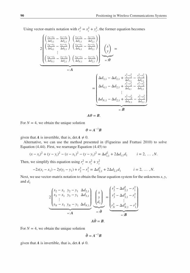
90 Positioning in Wireless Communications Systems
Using vector-matrix notation with r2i = x2
i + y2i , the former equation becomes
2
⎛⎜⎜⎜⎜⎜⎜⎝
(x3−x1
Δd3,1− x2−x1
Δd2,1
) (y3−y1
Δd3,1− y2−y1
Δd2,1
)(x4−x1
Δd4,1− x2−x1
Δd2,1
) (y4−y1
Δd4,1− y2−y1
Δd2,1
)⋮(
xN−x1
ΔdN,1− x2−x1
Δd2,1
) (yN−y1
ΔdN,1− y2−y1
Δd2,1
)⎞⎟⎟⎟⎟⎟⎟⎠
⏟⏞⏞⏞⏞⏞⏞⏞⏞⏞⏞⏞⏞⏞⏞⏞⏞⏞⏞⏞⏞⏞⏞⏞⏞⏞⏞⏞⏟⏞⏞⏞⏞⏞⏞⏞⏞⏞⏞⏞⏞⏞⏞⏞⏞⏞⏞⏞⏞⏞⏞⏞⏞⏞⏞⏞⏟=∶A
(xy
)⏟⏟⏟=∶𝜽
=
=
⎛⎜⎜⎜⎜⎜⎜⎝
Δd3,1 − Δd2,1 +r21−r2
3
Δd3,1−
r21−r2
2
Δd2,1
Δd4,1 − Δd2,1 +r21−r2
4
Δd4,1−
r21−r2
2
Δd2,1
⋮
ΔdN,1 − Δd2,1 +r21−r2
N
ΔdN,1−
r21−r2
2
Δd2,1
⎞⎟⎟⎟⎟⎟⎟⎠⏟⏞⏞⏞⏞⏞⏞⏞⏞⏞⏞⏞⏞⏞⏞⏞⏞⏞⏞⏞⏞⏞⏞⏟⏞⏞⏞⏞⏞⏞⏞⏞⏞⏞⏞⏞⏞⏞⏞⏞⏞⏞⏞⏞⏞⏞⏟
=∶B
A𝜽 = B.
For N = 4, we obtain the unique solution
𝜽 = A−1B
given that A is invertible, that is, detA ≠ 0.Alternative, we can use the method presented in (Figueiras and Frattasi 2010) to solve
Equation (4.44). First, we rearrange Equation (4.45) to
(x − xi)2 + (y − yi)2 − (x − x1)2 − (y − y1)2 = Δd2i,1 + 2Δdi,1d1 i = 2, … ,N.
Then, we simplify this equation using r2i = x2
i + y2i
−2x(xi − x1) − 2y(yi − y1) + r22− r2
1= Δd2
2,1 + 2Δd2,1d1 i = 2, … ,N.
Next, we use vector-matrix notation to obtain the linear equation system for the unknowns x, y,and d1
2
⎛⎜⎜⎜⎝x2 − x1 y2 − y1 Δd2,1
x3 − x1 y3 − y1 Δd3,1
⋮xN − x1 yN − y1 ΔdN,1
⎞⎟⎟⎟⎠⏟⏞⏞⏞⏞⏞⏞⏞⏞⏞⏞⏞⏞⏞⏞⏞⏞⏞⏟⏞⏞⏞⏞⏞⏞⏞⏞⏞⏞⏞⏞⏞⏞⏞⏞⏞⏟
=∶A
⎛⎜⎜⎝xyd1
⎞⎟⎟⎠⏟⏟⏟
=∶�̂�
=
⎛⎜⎜⎜⎜⎝r2
2− Δd2
2,1− r2
1
r23− Δd2
3,1− r2
1
⋮r2
N − Δd2N,1
− r21
⎞⎟⎟⎟⎟⎠⏟⏞⏞⏞⏞⏞⏞⏞⏞⏞⏟⏞⏞⏞⏞⏞⏞⏞⏞⏞⏟
=∶B
A�̂� = B.
For N = 4, we obtain the unique solution
�̂� = A−1B
given that A is invertible, that is, detA ≠ 0.
Position Estimation 91
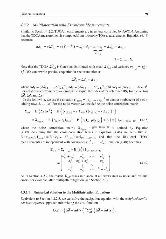
4.3.2 Multilateration with Erroneous Measurements
Similar to Section 4.2.2, TDOA measurements are in general corrupted by AWGN. Assumingthat the TDOA measurement is computed from two noisy TOA measurements, Equation (4.44)becomes
Δd̂i,1 = cΔT̂i,1 = c(T̂i − T̂1
)= di − d1 + 𝜖i − 𝜖1
⏟⏟⏟=∶𝜖i,1
= Δdi,1 + Δ𝜖i,1,
i = 2, … ,N.
Note that the TDOA Δd̂i,1 is Gaussian distributed with mean Δdi,1 and variance 𝜎2Δ𝜖i,1
= 𝜎2𝜖i+
𝜎2𝜖1
. We can rewrite previous equation in vector notation as
Δd̂1 = Δd1 + Δ𝝐1,
where Δd̂1 = (Δd̂2,1,… ,Δd̂N,1)T, Δd1 = (Δd2,1,… ,ΔdN,1)T, and Δ𝝐1 = (Δ𝜖2,1,… ,Δ𝜖N,1)T.For notational convenience, we omit in the sequel the index of the reference BS1 for the vectors
Δd̂, Δd, and Δ𝝐.
In the following, we use the notation 𝝐(2∶N) =(𝜖2, … , 𝜖N
)Tto denote a subvector of 𝝐 con-
taining rows 2, … ,N. For the noise vector Δ𝝐, we define the noise correlation matrix
𝚺Δ𝝐 = E{Δ𝝐Δ𝝐T
}= E
{(𝝐(2∶N) − 𝜖1𝟏N−1
) (𝝐(2∶N) − 𝜖1𝟏N−1
)T}
= 𝚺𝝐(2∶N)− E
{𝝐(2∶N)𝜖1𝟏T
N−1
}− E
{𝜖1𝟏N−1𝝐
T(2∶N)
}+ E
{𝜖2
1
}𝟏(N−1) × (N−1), (4.48)
where the noise correlation matrix 𝚺𝝐(2∶N)∈ ℝ(N−1)×(N−1) is defined by Equation
(4.39). Assuming that the cross-correlation terms in Equation (4.48) are zero, that is,
E{𝝐(2∶N)𝜖1𝟏T
N−1
}= E
{𝜖1𝟏N−1𝝐
T(2∶N)
}= 𝟎(N−1)×(N−1) and that the link-level ‘TOA’
measurements are independent with covariances 𝜎2𝜖1, … , 𝜎2
𝜖N, Equation (4.48) becomes
𝚺Δ𝝐 = 𝚺𝝐(2∶N)+ E
{𝜖2
1
}𝟏(N−1)×(N−1)
=⎛⎜⎜⎜⎝𝜎2𝜖1+ 𝜎2
𝜖2𝜎2𝜖1
· · · 𝜎2𝜖1
𝜎2𝜖1
𝜎2𝜖1+ 𝜎2
𝜖3· · · 𝜎2
𝜖1
⋮ ⋮ ⋱ ⋮𝜎2𝜖1
𝜎2𝜖1
· · · 𝜎2𝜖1+ 𝜎2
𝜖N
⎞⎟⎟⎟⎠ . (4.49)
As in Section 4.2.2, the matrix 𝚺Δ𝝐 takes into account all errors such as noise and residualerrors, for example, after multipath mitigation (see Section 7.3).
4.3.2.1 Numerical Solution to the Multilateration Equations
Equivalent to Section 4.2.2.3, we can solve the navigation equation with the weighted nonlin-ear least squares approach minimizing the cost function
L (x) =(Δd̂ − Δd (x)
)T𝚺−1
Δ𝝐
(Δd̂ − Δd (x)
).

92 Positioning in Wireless Communications Systems
with respect to the unknown MT position. Here, Δd̂ ∈ ℝN−1 includes the N − 1 measuredTDOAs and Δd (x) the ideal, real TDOAs. As before, a suitable algorithm provides the MTposition estimate
x̂ = argminx
L (x) .
In general, there exists no analytical solution to this nonlinear two or three-dimensional prob-lem. Hence, we have to apply iterative algorithms.
Gauss–Newton AlgorithmAs for solving the trilateration navigation equations, we can apply the Gauss–Newton algo-rithm (Foy 1976) to solve the multilateration navigation equations. In this case, the lineariza-tion step is given by
Δd (x) ≈ Δd(x(0)
)+𝚽 (x) |x=x(0) (x − x(0)
)with the elements of the (N − 1) × 2 Jacobian matrix
𝚽 (x) = ∇xT ⊗ Δd (x) =
⎛⎜⎜⎜⎜⎜⎝
x−x2
d2− x−x1
d1
y−y2
d2− y−y1
d1
x−x3
d3− x−x1
d1
y−y3
d3− y−y1
d1
⋮ ⋮x−xN
dN− x−x1
d1
y−yN
dN− y−y1
d1
⎞⎟⎟⎟⎟⎟⎠,
where ∇x =(
𝜕
𝜕x, 𝜕
𝜕y
)T. Similar to Section 4.2.2.3, the linear least squares method is applied
resulting in the iterated Gauss–Newton algorithm
x̂(k+1) = x̂(k) +(𝚽T
(x̂(k)
)𝚺−1Δ𝝐𝚽
(x̂(k)
)−1)
⏟⏞⏞⏞⏞⏞⏞⏞⏞⏞⏞⏞⏞⏞⏞⏞⏞⏞⏟⏞⏞⏞⏞⏞⏞⏞⏞⏞⏞⏞⏞⏞⏞⏞⏞⏞⏟
A(k),−1TDOA
𝚽T(x̂(k)
)𝚺−1Δ𝝐
(Δd̂ − Δd
(x̂(k)
))⏟⏞⏞⏞⏞⏞⏞⏞⏞⏞⏞⏞⏞⏞⏞⏞⏞⏞⏞⏞⏞⏞⏞⏟⏞⏞⏞⏞⏞⏞⏞⏞⏞⏞⏞⏞⏞⏞⏞⏞⏞⏞⏞⏞⏞⏞⏟
=∶g(k)TDOA
= x̂(k) + A(k),−1
TDOAg(k)
TDOA.
Note that the noise correlation matrix for TDOAs 𝚺Δ𝝐 in this equation always containsnon-zero off-diagonal entries (see Equations 4.48 and 4.49) in contrast to the noise correlation
matrix for TOAs (see Equations 4.39 and 4.40). Thus, the matrix A(k)TDOA
can become singularfor bad geometric conditions or bad initial values. Then, the Gauss–Newton algorithm can
have convergence problems due to such an ill-conditioned matrix A(k)TDOA
. For these scenarios,the hyperbolic character of the TDOA measurements needs more robust approaches. Two ofthem are presented next.
Steepest Descent AlgorithmIn contrast to Gauss–Newton, the gradient based steepest descent algorithm with search direc-tion ∇x = L (x) and step size 𝜇 yields
x̂(k+1) = x̂(k) + 𝜇(k)𝚽T(x̂(k)
)𝚺−1Δ𝝐
(Δd̂ − Δd
(x̂(k)
))⏟⏞⏞⏞⏞⏞⏞⏞⏞⏞⏞⏞⏞⏞⏞⏞⏞⏞⏞⏞⏞⏞⏞⏟⏞⏞⏞⏞⏞⏞⏞⏞⏞⏞⏞⏞⏞⏞⏞⏞⏞⏞⏞⏞⏞⏞⏟
=∶g(k)TDOA
= x̂(k) + 𝜇(k)g(k)TDOA
.

Position Estimation 93
The step size can be either chosen constant 𝜇(k) = 𝜇 for all iterations or a line-search procedurecan be performed to find the optimum step size per iteration. As in Section 4.2.2.3, the maindrawbacks of the steepest descent method are the possibility of running in local minima andslow convergence in the final iterations.
Levenberg–Marquardt AlgorithmTo cope with the problems of Gauss–Newton and steepest descent (robustness and slow con-vergence), the Levenberg–Marquardt algorithm is adapted to the TDOA-based positioningproblem (Mensing and Plass 2006), that is,
x̂(k+1) = x̂(k) +(𝚽T
(x̂(k)
)𝚺−1Δ𝝐𝚽
(x̂(k)
)⏟⏞⏞⏞⏞⏞⏞⏞⏞⏞⏞⏞⏞⏞⏟⏞⏞⏞⏞⏞⏞⏞⏞⏞⏞⏞⏞⏞⏟
A(k)TDOA
+ 𝜆(k)I2
)−1
⋅
𝚽T(x̂(k)
)𝚺−1Δ𝝐
(Δd̂ − Δd
(x̂(k)
))⏟⏞⏞⏞⏞⏞⏞⏞⏞⏞⏞⏞⏞⏞⏞⏞⏞⏞⏞⏞⏞⏞⏞⏟⏞⏞⏞⏞⏞⏞⏞⏞⏞⏞⏞⏞⏞⏞⏞⏞⏞⏞⏞⏞⏞⏞⏟
=∶g(k)TDOA
= x̂(k) +(A(k)
TDOA+ 𝜆(k)I2
)− 1g(k)
TDOA.
Similar to TOA in Section 4.2.2.3, the damping parameter 𝜆(k) ensures that the appropriatematrix–in comparison to Gauss–Newton–can always be inverted yielding a much more robustimplementation.
4.4 Fingerprinting
In Section 2.3, we introduced the fingerprinting positioning method. We defined a fingerprintin wireless positioning as a set of measurable signal characteristics that depend on the posi-tion of transmission or reception. Thus, the previously considered AOA, AOAD, RSS, TOA,and TDOA measurements are wireless fingerprints. In general, fingerprinting also considersmeasurements that cannot be expressed through explicit functional relations between the loca-tion dependent measurements and the MT position. Therefore, fingerprinting usually buildsup a database, which contains the fingerprints, that is, the set of signal characteristics for eachposition in the environment. The database is often created in an off-line phase. During theonline phase, a fingerprinting method then compares a measured fingerprint to the fingerprintentries of that database in order to determine the database fingerprint that matches best andthus, the corresponding MT position. Consequently, the fingerprinting database can be seen asa generalization of the previously presented navigation equations.
Many different algorithms for fingerprinting exist (Liu et al. 2007a), which can be classi-fied as probabilistic, k-nearest neighbor, neural network, support vector machine, or smallestM-vertex polygon algorithms.
The probabilistic algorithms determine for each measurement in the database and for theactual measurement a probability that the measured fingerprint corresponds to a specific loca-tion. Then, the algorithm chooses the location with the highest probability.
The k-nearest neighbor algorithms use the online measured fingerprint to determine from thedatabase k closest matching fingerprints. From these fingerprints, the algorithm then estimatesan average position.

94 Positioning in Wireless Communications Systems
Neural network algorithms learn during the off-line phase the implicit relation between thefingerprints and the measured locations by obtaining appropriate weights. During the onlinephase these weights are applied to the measured fingerprints to estimate the MT position.
For further details on fingerprinting algorithms, we refer the interested reader to (Liu et al.2007a) and references therein.
4.5 Performance Bounds and Measures
This section presents some performance bounds and measures to asses the accuracy of thepreviously presented positioning algorithms. Specifically, we consider the positioning rootmean square error (RMSE), the cumulative distribution function (CDF) and the circular errorprobability (CEP) of the positioning error, the positioning CRLB, the dilution of precision(DOP), and the complexity.
4.5.1 Root Mean Square Error–RMSE
The RMSE of an position estimator x̂ is defined as
𝜖RMSE =√
E{||x − x̂||22}.
Note that the RMSE takes into account both the variance and the bias of an estimator, that is,
𝜖2RMSE
= VAR {x̂} + ||Bias (x̂)||22 with
VAR {x̂} = E{||x̂ − E {x̂}||22} and Bias (x̂) = E {x̂} − x.
Thus, we can compare through the RMSE both biased and unbiased estimators.
4.5.2 Cumulative Distribution Function – CDF
With the CDF, usually outage probabilities can be analyzed, that is, at what probability willa positioning method fail to achieve a certain accuracy. The CDF of the positioning error in[m] is defined as the probability that the absolute two-dimensional position error is below thevalue ‘error’, that is,
CDF (error) = P(||x − x̂||2 ≤ error
).
The CDF is usually obtained over several MT positions and noise realizations, for example,Section 5.3.
4.5.3 Circular Error Probability–CEP
The CEP is defined as the probability for which a measurement will fall into a circle withradius r (Gustafsson and Gunnarsson 2005)
CEPp (r) = P(||x − x̂||2 < r
)= p.
Typical CEPs are p = 67% and p = 95%.
Position Estimation 95
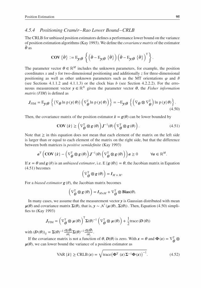
4.5.4 Positioning Cramér–Rao Lower Bound–CRLB
The CRLB for unbiased position estimators defines a performance lower bound on the varianceof position estimation algorithms (Kay 1993). We define the covariance matrix of the estimator�̂� as
COV{�̂�}∶= Ey|𝜽
{(�̂� − Ey|𝜽 {
�̂�})(
�̂� − Ey|𝜽 {�̂�})T
}.
The parameter vector 𝜽 ∈ ℝM includes the unknown parameters, for example, the positioncoordinates x and y for two-dimensional positioning and additionally z for three-dimensionalpositioning as well as other unknown parameters such as the MT orientations 𝜑 and 𝜗(see Sections 4.1.1.2 and 4.1.1.3) or the clock bias b (see Section 4.2.2.2). For the erro-neous measurement vector y ∈ ℝN given the parameter vector 𝜽, the Fisher informationmatrix (FIM) is defined as
JFIM = Ey|𝜽 {(∇𝜽 ln p (y|𝜽)) (∇T
𝜽ln p (y|𝜽))} = −Ey|𝜽 {(
∇𝜽 ⊗ ∇T
𝜽
)ln p (y|𝜽)} .
(4.50)
Then, the covariance matrix of the position estimator x̂ = g(𝜽) can be lower bounded by
COV {x̂} ≥ (∇T
𝜽⊗ g (𝜽)
)J−1(𝜽)
(∇T
𝜽⊗ g (𝜽)
). (4.51)
Note that ≥ in this equation does not mean that each element of the matrix on the left sideis larger than or equal to each element of the matrix on the right side, but that the differencebetween both matrices is positive semidefinite (Kay 1993)
aT(
COV {x̂} −(∇T
𝜽⊗ g (𝜽)
)J−1(𝜽)
(∇T
𝜽⊗ g (𝜽)
))a ≥ 0 ∀a ∈ ℝM .
If x = 𝜽 and g (𝜃) is an unbiased estimator, i.e. E {g (𝜽)} = 𝜽, the Jacobian matrix in Equation(4.51) becomes (
∇T
𝜽⊗ g (𝜽)
)= IM × M .
For a biased estimator g (𝜃), the Jacobian matrix becomes(∇T
𝜽⊗ g (𝜽)
)= IM×M + ∇T
𝜽⊗ Bias(𝜽).
In many cases, we assume that the measurement vector y is Gaussian distributed with mean𝝁(𝜽) and covariance matrix 𝚺(𝜽), that is, y ∼ (𝝁 (𝜽) ,𝚺(𝜽)) . Then, Equation (4.50) simpli-fies to (Kay 1993)
JFIM =(∇T
𝜽⊗ 𝝁 (𝜽)
)T
𝚺(𝜽)−1(∇T
𝜽⊗ 𝝁 (𝜽)
)+ 1
2trace (D (𝜽))
with (D (𝜽))ij = 𝚺(𝜽)−1 𝜕𝚺(𝜽)𝜕𝜃i
𝚺(𝜽)−1 𝜕𝚺(𝜽)𝜕𝜃j
.
If the covariance matrix is not a function of 𝜽, D(𝜽) is zero. With x = 𝜽 and 𝚽 (x) = ∇T
𝜽⊗
𝝁(𝜽), we can lower bound the variance of a position estimator as
VAR {x̂} ≥ CRLB (x) =√
trace(𝚽T (x)𝚺−1𝚽 (x)
)−1. (4.52)

96 Positioning in Wireless Communications Systems
Here, x, 𝚽 (x), and 𝚺 denote the M-dimensional position vector, the N × M Jacobian matrix
of the measurement model, which takes into account the geometry of the BSs and MT, and
the N × N noise covariance matrix of the measurements. Thus, the CRLB takes into account
the geometry of the considered scenario, the measurement accuracies, and the measurement
dependencies.
Figure 4.7 shows the positioning CRLB for trilateration (TOA) without and with clock
bias, multilateration (TDOA), and triangulation (AOA). We calculated the CRLB according
to (4.52) for TOA and AOA measurements with 𝜎2𝜖i= 1 m and 𝜎2
𝜑𝜖i= 0.01∘. For triangulation,
we analyze the downlink AOA with unknown MT orientation according to Equations (4.6),
(4.7), and (4.9). The maximum plotted variance of the estimated position is 3 m. Comparing
the different methods, clearly the trilateration with TOAs and no clock bias provides the best
accuracy for this scenario. Both TOA with clock bias and TDOA provide only a good accuracy
within the triangle formed by the three BSs. Note that the CRLBs for TOA and TDOA are the
same in accordance with (Urruela et al. 2006) although the gray shading is not exactly the same
due to some numerical effects along the x-axis for TDOA. To achieve a similar performance
with the triangulation methods as with TDOA, we have to choose 𝜎2𝜑𝜖i
= 0.01∘. The CRLBs
for downlink AOA and AOAD with unknown MT orientation and the nonlinear arctan func-
tion from Equations (4.6) and (4.7) are the same similar to TOA with clock bias and TDOA.
In contrast the CRLB for downlink AOAD with unknown MT orientation and the arccos from
Equation (4.9) is different due to the different nonlinear functions.
4.5.5 Dilution of Precision–DOP
The DOP is strongly related to the CRLB. With DOP the geometric influence of the positioning
scenario on the overall positioning performance is described. For trilateration with unknown
MT clock bias, the matrix
Ξ =(𝚽T (x)𝚽 (x)
)−1 =⎛⎜⎜⎜⎝EDOP2 ⋅ ⋅ ⋅
⋅ NDOP2 ⋅ ⋅⋅ ⋅ VDOP2 ⋅⋅ ⋅ ⋅ TDOP2
⎞⎟⎟⎟⎠can be separated in different DOP parts: east DOP (EDOP), north DOP (NDOP), verticalDOP (VDOP), and time DOP (TDOP). Hence, the position DOP (PDOP) is defined as
PDOP =√
EDOP2 + NDOP2 + VDOP2,
and the overall DOP or geometric DOP (GDOP) is defined as
DOP = GDOP =√
PDOP2 + TDOP2 =√
trace (Ξ).
The DOP analysis can help to estimate the expected RMSE if the measurement accuracy on
all links is assumed equal. Then, the DOP is due to geometrical properties of the current
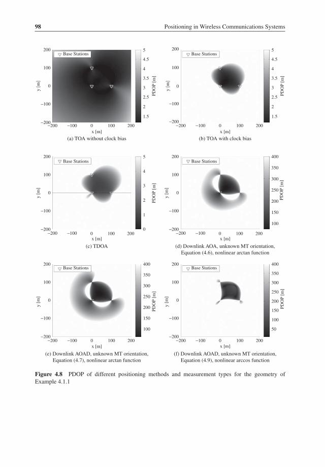
scenario. For instance, Figure 4.8 compares the PDOP of different positioning methods and
measurement types for the geometry of Example 4.1.1. Similar to the CRLBs in Figure 4.7, the
trilateration method for TOA without clock bias shows the best performance. For the PDOP,
the performance of TDOA is better than that of TOA with clock bias in Figure 4.8, which is

Position Estimation 97
200
100
y [m
]
−100
−200−200 −100 0
x [m]
(a) TOA without clock bias
100 200
0
3
2.5
CR
LB
[m
]
1.5
2
200Base Stations
100
y [m
]
−100
−200−200 −100 0
x [m]
(b) TOA with clock bias
x [m]
(c) TDOA
x [m]
(d) Downlink AOA, unknown MT orientation,
Equation (4.6), nonlinear arctan function
x [m]
(e) Downlink AOAD, unknown MT orientation,
Equation (4.7), nonlinear arctan function
x [m]
(f) Downlink AOAD, unknown MT orientation,
Equation (4.9), nonlinear arccos function
100 200
0
3
2.5
CR
LB
[m
]
1.5
2
200
100
y [m
]
−100
−200−200 −100 0 100 200
0
3
2
2.5C
RL
B [m
]
0.5
0
1.5
1
200Base Stations
100y [m
]
−100
−200−200 −100 0 100 200
0
3
2.5
CR
LB
[m
]
1.5
1
2
200
100
y [m
]
−100
−200−200 −100 0 100 200
0
3
2.5
CR
LB
[m
]
1.5
1
2
200Base Stations
Base Stations
Base Stations
Base Stations
100
y [m
]
−100
−200−200 −100 0 100 200
0
3
2.5
2
CR
LB
[m
]
1
0.5
1.5
Figure 4.7 Positioning CRLB of different positioning methods and measurement types for the geom-
etry of Example 4.1.1, 𝜎2𝜖i= 1 m for TOA measurements and 𝜎2
𝜑𝜖i= 0.01∘ for AOA measurements
98 Positioning in Wireless Communications Systems
200
100
y [m
]
−100
−200−200 −100 0
x [m]
(a) TOA without clock bias
100 200
0
5
4
4.5
PD
OP
[m
]P
DO
P [m
]P
DO
P [m
]
1.5
2
2.5
3
3.5
5
4
4.5
PD
OP
[m
]P
DO
P [m
]
1.5
2
2.5
3
3.5
200Base Stations
100
y [m
]
−100
−200−200 −100 0
x [m]
(b) TOA with clock bias
x [m]
(c) TDOA
x [m]
(e) Downlink AOAD, unknown MT orientation,
Equation (4.7), nonlinear arctan function
(f) Downlink AOAD, unknown MT orientation,
Equation (4.9), nonlinear arccos function
100 200
0
200
100
y [m
]
−100
−200−200 −100 0 100 200
0
5
4
1
0
3
2
200
y [m
]
0
−100
−200−200 −100 0 100 200
100
400
250
200
150
100
350
300
x [m]
200
y [m
]
0
−100
−200−200 −100 0 100 200
100
400
200
150
100
50
300
350
250
PD
OP
[m
]
x [m]
(d) Downlink AOA, unknown MT orientation,
Equation (4.6), nonlinear arctan function
200
100
y [m
]
−100
−200−200 −100 0 100 200
0
400
350
150
100
250
300
200
Base Stations
Base Stations
Base Stations Base Stations
Base Stations
Figure 4.8 PDOP of different positioning methods and measurement types for the geometry of
Example 4.1.1
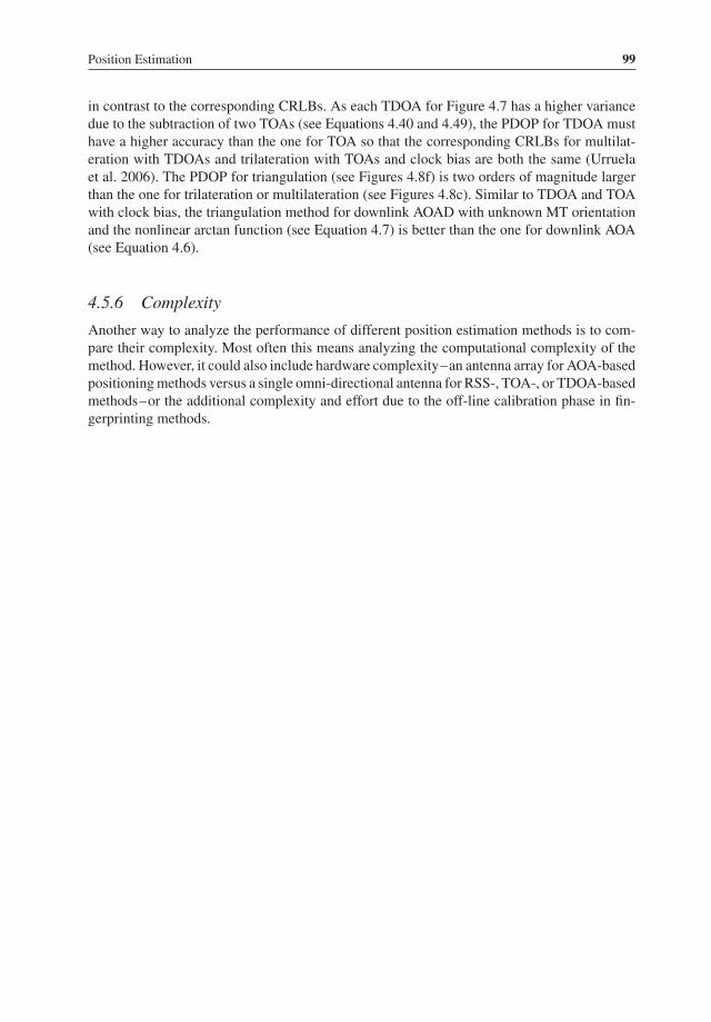
Position Estimation 99
in contrast to the corresponding CRLBs. As each TDOA for Figure 4.7 has a higher variance
due to the subtraction of two TOAs (see Equations 4.40 and 4.49), the PDOP for TDOA must
have a higher accuracy than the one for TOA so that the corresponding CRLBs for multilat-
eration with TDOAs and trilateration with TOAs and clock bias are both the same (Urruela
et al. 2006). The PDOP for triangulation (see Figures 4.8f) is two orders of magnitude larger
than the one for trilateration or multilateration (see Figures 4.8c). Similar to TDOA and TOA
with clock bias, the triangulation method for downlink AOAD with unknown MT orientation
and the nonlinear arctan function (see Equation 4.7) is better than the one for downlink AOA
(see Equation 4.6).
4.5.6 Complexity
Another way to analyze the performance of different position estimation methods is to com-
pare their complexity. Most often this means analyzing the computational complexity of the
method. However, it could also include hardware complexity–an antenna array for AOA-based
positioning methods versus a single omni-directional antenna for RSS-, TOA-, or TDOA-based
methods–or the additional complexity and effort due to the off-line calibration phase in fin-
gerprinting methods.