porosity concepts in gassmann fluid substitution: a

Third EAGE Workshop on Rock Physics 15-18 November 2015, Istanbul, Turkey

RP06Porosity Concepts in Gassmann FluidSubstitution: A Simulator to Seismic ModellingPerspectiveH. Amini* (Heriot-Watt University) & C. MacBeth (Heriot-Watt University)

SUMMARYIn this study, porosity concepts in Gassmann’s fluid substitution model are examined and theirimplications for quantitative 4D seismic studies are discussed. Three porosity models (total porosity,effective porosity, and a movable fluid model) are compared from a simulator to seismic (sim2seis)modelling perspective. From the three selected models, total porosity predicts the largest softening effectdue to gas breakout and the smallest hardening effect from water-flooding; whereas the movable fluidmodel predicts the least softening due to gas breakout and the largest effects for water-flooding. Effectiveporosity predictions lie between the total porosity and movable fluid models. The differences betweenthese models are due to the proportion of fluids in the mixture which are input into Gassmann’s equations.Sim2seis results based on different porosity models were evaluated against the observed 4D seismic. Thiscomparison shows that the magnitude of the saturation-induced hardening and softening signals due to themovable fluid model is closer to the observed seismic. The total porosity model is in least agreement withthe observed 4D seismic.


Introduction

Fluid substitution is an essential part of the petro-elastic modelling (PEM) for 4D seismic studies. It concerns the prediction of changes in density and elastic moduli of saturated rocks due to the changes in pore fluid phases or changes in the acoustic properties of the existing fluids. Gassmann’s model is by far the most common theory used for fluid substitution. It is appreciated in the literature that different porosity choices (total or effective) exist for Gassmann fluid substitution (May 2005). However, a thorough assessment of these models is not covered, and approaches attempt to validate Gassmann’s model with little reference to the underlying porosity models. In addition to total and effective porosity, a third choice – here, referred to as the “movable fluid model” – also exists for porosity in Gassmann’s model. In this study, the 4D seismic responses of the three porosity models (total porosity, effective porosity, and movable fluid model) are examined in an application of the petro-elastic model to a simulation model from a deep-water turbidite reservoir in the UKCS West of Shetland region. Simulator to seismic modelling (sim2seis) is used to compare the synthetic 4D seismic amplitude maps based on the different porosity models with the observed 4D seismic response.

Methods and application

Following Wang (2001), Gassmann’s model requires that the pore fluid pressure induced by the passing wave be in full equilibrium within the time-frame of half of a seismic wave period. To fulfil this criterion, all the pores need to be interconnected. Wang (2001) and Simm (2007) reported that the effective porosity model fulfils the underlying assumptions of Gassmann’s theory regarding full pore-space interconnectivity, and the clay-bound water should be considered as a part of the dry-frame. However, using numerical and analytical analyses, Grechka (2009) showed that under some conditions (aspect ratios of the pores greater than approximately 0.2), the presence of disconnected porosity is unlikely to invalidate Gassmann’s model predictions. The use of total porosity has also been reported in a number of fluid substitution studies and laboratory measurements (e.g. Grochau and Gurevich 2009). It should be noted that maintaining the effective porosity conditions for laboratory measurements is difficult; hence, most laboratory measurements tend to be based on total porosity (Taggart 2002).

Yan et al. (2013) suggested that the porosity in Gassmann’s equation should include the volume fraction of pore fluids that is connected and relaxed, while the other fraction of pore fluids should be included in the rock matrix. They used irreducible water saturation to quantify the pore fluids that cannot be driven out by hydraulic force. In fact, similar to clay-bound water, capillary-bound fluids will not be replaced during fluid substitution. One can therefore limit the fluid substitution exercise to the portion of the pore space occupied by movable fluids only. In this setting, both the clay-bound water and capillary-bound fluids are considered to be a part of the rock frame. The uncertainties associated with the estimation of the irreducible fluids volume fractions is one of the issues in the application of the movable fluid model. Matthews et al. (2013) utilised the movable fluids model in a fluid substitution exercise. They reported that, compared to the effective porosity model, this model derives a more reasonable range for the dry-frame bulk moduli. Also, by replacing gas with brine, they reported a lower fluid effect (i.e. less change in impedance) compared to the model based on effective porosity, and argued that the results based on the movable fluid model are more realistic.

The petrophysical definitions of the three porosity models and their corresponding components for the Gassmann’s model are shown in Figure 1. Simulator to seismic (sim2seis) modelling is used here to examine the synthetic 4D response based on these models. The pore volume fraction in the geomodel is equivalent to the effective porosity. To calculate the total porosity, the volume fraction of the clay-bound water is estimated using a multi-linear regression based on and and added to the effective porosity. To calculate the volume fraction of the movable fluids, the saturation end members based on the relative permeability curves are used to exclude the volume fractions of the capillary-bound fluids from effective porosity.


Modelling results

The results of applying PEM to the simulation model for the three porosity models are shown in Table 1 and Figure 2. The movable fluids model predicts a higher impedance change due to oil being replaced by water; however, in the case of gas breakout, the movable fluids model has lower impedance change. As shown in Figure 3, the differences between these models are mainly due to the different values of effective bulk modulus of fluids ( ) in each case due to the different proportion of fluid phases. Matthews et al. (2013) also reported a similar response of the movable fluids model for gas being replaced by water. Nonetheless, it is clear that their generalisation of the gas response to fluids, in stating that the ‘movable fluids model represents a lower magnitude of fluid effects’, is not applicable to the case where oil is replaced with water.

Comparison with the observed data

Figure 4 compares the observed 4D amplitude map with the sim2seis results based on the three porosity models. In the observed 4D map (Figure 4a), the absolute value of the amplitude changes due to water-flooding signals (in blue circles) and gas breakout signals (in red circles) are comparable. On the other hand, in the sim2seis results (Figure 4b-d), the gas breakout signal appears to have a higher amplitude compared to the water-flooding signal. However, by comparison, the magnitude of the hardening and softening signals for movable fluid model (Figure 4d) are closer to the observed 4D map. The total porosity model is in least agreement with the observed 4D seismic, where the absolute value of the amplitude changes due to gas breakout is much higher than the amplitude change due to water-flooding.

Conclusions and discussions

Three porosity models, (total, effective, and movable fluid models) were adapted for Gassmann’s fluid substitution model. From these three models, total porosity predicted the largest softening due to gas breakout and the smallest hardening effect from water-flooding; whereas the movable fluid model predicted the least softening due to gas breakout and the largest effects for water-flooding. Sim2seis results based on these porosity models were evaluated against the observed 4D seismic. This comparison shows that the magnitude of the saturation induced hardening and softening signals for the movable fluid model are the closest to the observed seismic, whereas the total porosity model is in least agreement with the observed 4D seismic data.

Acknowledgments

We thank the sponsors of the Edinburgh Time Lapse Project, Phase V, for their support (BG, BP, Chevron, CGG, ConocoPhillips, ENI, ExxonMobil, Hess, Ikon Science, Landmark, Maersk, Norsar, RSI, Nexen, Petoro, Petrobras, Shell, Statoil, Suncor, Taqa, TGS and Total). Thanks are extended to Schlumberger for providing the Petrel and Eclipse software.

References

Grechka V. 2009. Fluid-solid substitution in rocks with disconnected and partially connected porosity. Geophysics 74, WB89-WB95.

Grochau M. and Gurevich B. 2009. Testing Gassmann fluid substitution: sonic logs versus ultrasonic core measurements. Geophysical Prospecting 57, 1365-2478.

Hook J.R. 2003. An introduction to porosity. Petrophysics 44, 205-212. Matthews S.A., Lovell M.A., Davies S.J., Pritchard T., Abdelkarim A. and Sirju C. 2013. Fluid

substitution in laminated sand-shale sequences: an innovative approach to Gassmann’s equation. Petroleum Geoscience Conference & Exhibition, Kuala Lumpur, Malaysia.

May A. 2005. Using wet shale and effective porosity in a petrophysical velocity model. Offshore Technology Conference, Houston, Texas. OTC No. 17643-MS.

Simm R. 2007. Practical Gassmann fluid substitution in sand/shale sequences. First Break 25, 61-68. Taggart I. 2002. Effective versus total porosity based geostatistical models: Implications for upscaling

and flow simulations. Transport in Porous Media 46, 251-268. Wang Z. 2001. Fundamentals of seismic rock physics. Geophysics 66, 398-412.


Yan F., Han D. and Yao Q. 2013. Effective porosity for Gassmann fluid substitution. 83rd SEG meeting, Houston, USA, Expanded Abstracts, 2861-2865.

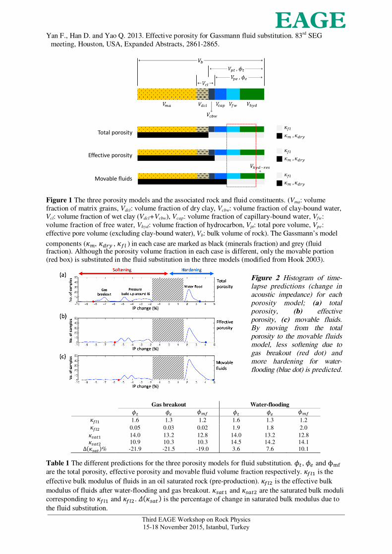
Figure 1 The three porosity models and the associated rock and fluid constituents. (Vma: volume fraction of matrix grains, Vdcl: volume fraction of dry clay, Vcbw: volume fraction of clay-bound water, Vcl: volume fraction of wet clay (Vdcl+Vcbw), Vcap: volume fraction of capillary-bound water, Vfw: volume fraction of free water, Vhyd: volume fraction of hydrocarbon, Vpt: total pore volume, Vpe: effective pore volume (excluding clay-bound water), Vb: bulk volume of rock). The Gassmann’s model

components ( , , ) in each case are marked as black (minerals fraction) and grey (fluid fraction). Although the porosity volume fraction in each case is different, only the movable portion (red box) is substituted in the fluid substitution in the three models (modified from Hook 2003).

Figure 2 Histogram of time-lapse predictions (change in acoustic impedance) for each porosity model; (a) total porosity, (b) effective porosity, (c) movable fluids. By moving from the total porosity to the movable fluids model, less softening due to gas breakout (red dot) and more hardening for water-flooding (blue dot) is predicted.

Gas breakout Water-flooding

1.6 1.3 1.2 1.6 1.3 1.20.05 0.03 0.02 1.9 1.8 2.0

14.0 13.2 12.8 14.0 13.2 12.8 10.9 10.3 10.3 14.5 14.2 14.1% -21.9 -21.5 -19.0 3.6 7.6 10.1

Table 1 The different predictions for the three porosity models for fluid substitution. , and are the total porosity, effective porosity and movable fluid volume fraction respectively. is the effective bulk modulus of fluids in an oil saturated rock (pre-production). is the effective bulk modulus of fluids after water-flooding and gas breakout. and are the saturated bulk moduli corresponding to and . is the percentage of change in saturated bulk modulus due tothe fluid substitution.


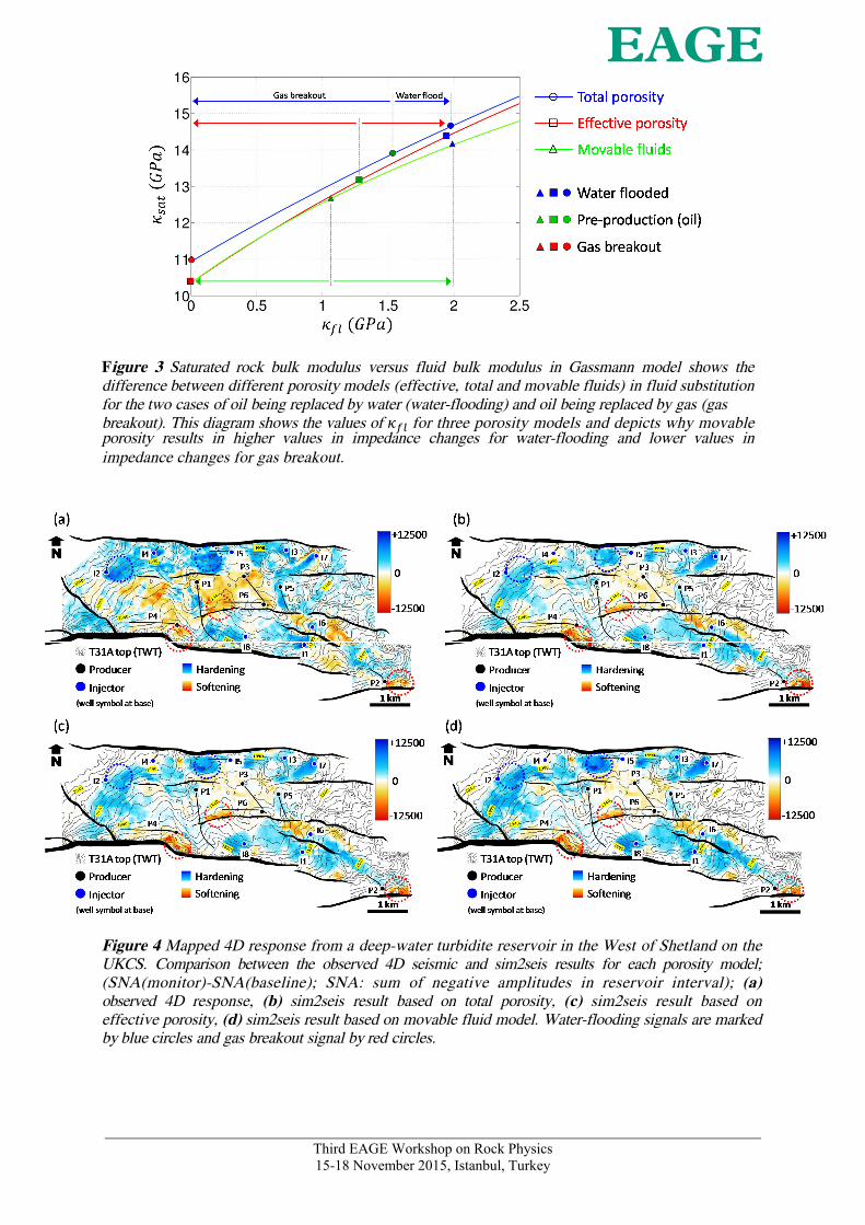
Figure 3 Saturated rock bulk modulus versus fluid bulk modulus in Gassmann model shows the difference between different porosity models (effective, total and movable fluids) in fluid substitution for the two cases of oil being replaced by water (water-flooding) and oil being replaced by gas (gas breakout). This diagram shows the values of for three porosity models and depicts why movable porosity results in higher values in impedance changes for water-flooding and lower values in impedance changes for gas breakout.

Figure 4 Mapped 4D response from a deep-water turbidite reservoir in the West of Shetland on the UKCS. Comparison between the observed 4D seismic and sim2seis results for each porosity model; (SNA(monitor)-SNA(baseline); SNA: sum of negative amplitudes in reservoir interval); (a) observed 4D response, (b) sim2seis result based on total porosity, (c) sim2seis result based on effective porosity, (d) sim2seis result based on movable fluid model. Water-flooding signals are marked by blue circles and gas breakout signal by red circles.

porosity concepts in gassmann fluid substitution: a

Documents