population structure of striped marlin kajikia audax) in ...appraise the presence of distinct stocks...

Population structure of striped marlin(Kajikia audax) in the Pacific Ocean based onanalysis of microsatellite and mitochondrial DNA

Jan R. McDowell and John E. Graves

Abstract: Genetic variation was surveyed at five microsatellite loci and the mitochondrial control region (819 bp) to testfor the presence of genetic stock structure in striped marlin (Kajikia audax) collections taken from seven locations through-out the Pacific Ocean. Temporal replicates separated by 9 years were taken off Japan, and three temporal samples spanning11 years were collected off the coast of eastern Australia. Analyses of multilocus microsatellite genotypes and mitochon-drial control region sequences showed no significant heterogeneity among collections taken from the same location in dif-ferent years; however, significant spatial genetic heterogeneity was observed across all samples for microsatellite markers(FST = 0.013, P < 0.001). Mitochondrial control region sequences were not different across all samples (�ST = –0.01, P =0.642). Analyses of molecular variance (AMOVA) revealed significant genetic differentiation between geographic regionsfor both microsatellite and mitochondrial markers. These results suggest the presence of genetically discrete populationswithin the Pacific Ocean and are supported by both the results of tagging studies, which show limited dispersal, and thepresence of geographically separated spawning grounds.

Resume : Nous avons analyse la variation genetique a cinq locus microsatellites et dans la region mitochondriale de con-trole (819 pb) pour verifier la presence de structure genetique dans des echantillons de stocks de marlins rayes (Kajikia au-dax) provenant de sept sites repartis dans tout le Pacifique. Nous avons pris des echantillons temporels a un intervalle de9 annees au large du Japon et trois echantillons temporels sur une periode de 11 ans au large de la cote de l’Australie ori-entale. Des analyses des genotypes a locus microsatellites multiples et des sequences de la region mitochondriale de con-trole n’indiquent aucune heterogeneite significative entre les recoltes prises au meme site durant des annees differentes; onobserve, cependant, une heterogeneite genetique spatiale significative parmi l’ensemble des echantillons chez les mar-queurs microsatellites (FST = 0,013, P < 0,001). Les sequences des regions mitochondriales de controle ne different pasdans l’ensemble des echantillons (�ST = –0,01, P = 0,642). Des analyses de la variance moleculaire (AMOVA) montrentune differenciation genetique significative entre les regions geographiques, tant chez les marqueurs microsatellites quemitochondriaux. Ces resultats font croire a l’existence de populations genetiquement distinctes au sein du Pacifique, ce quiest corrobore a la fois par les resultats des etudes de marquage qui revelent une dispersion limitee et par la presence desites de fraie separes geographiquement.

[Traduit par la Redaction]

Introduction

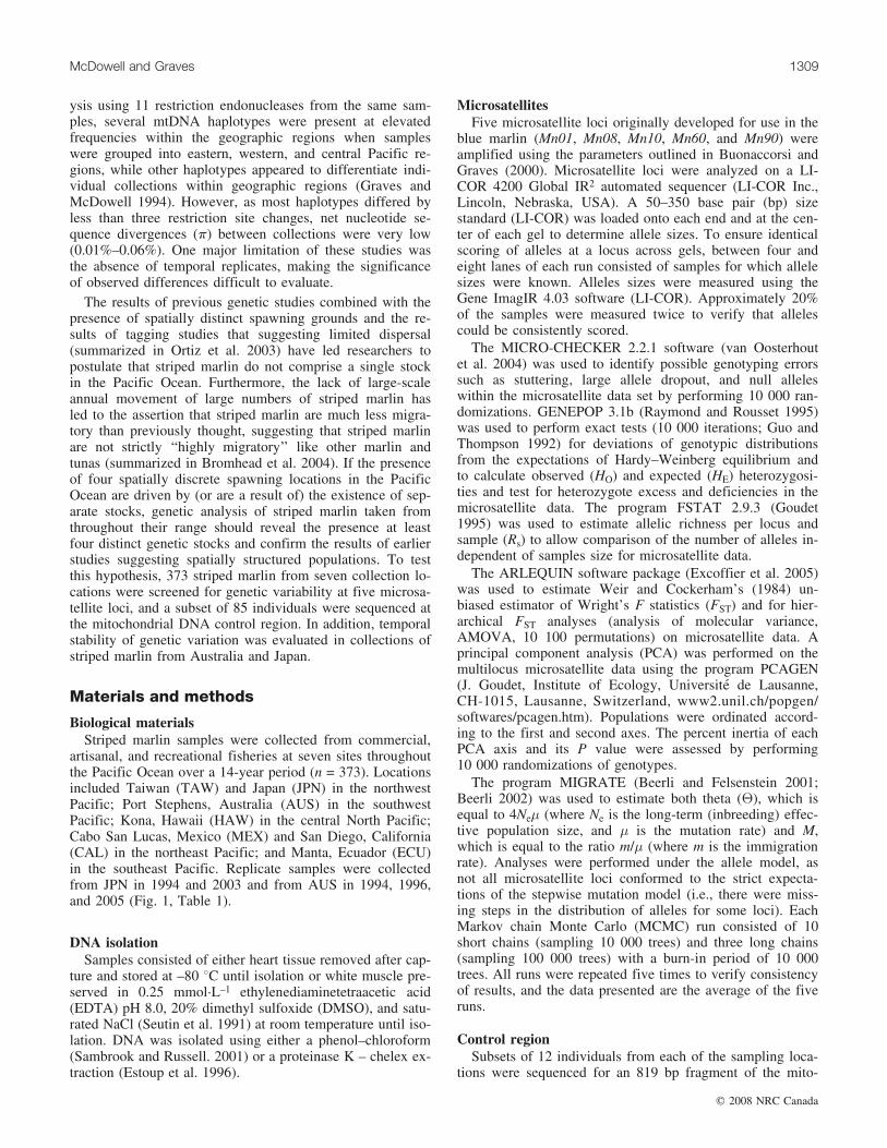
The factors leading to population structure in large pela-gic species, such as istiophorid billfishes, have been subjectto much speculation. Unlike less mobile organisms, pelagicspecies have a vast potential for dispersal and a lack ofapparent physical barriers (Graves 1998). In theory, thesefactors are thought to preclude the development of popula-tion genetic structure (Waples 1998; Smedbol et al. 2002).In addition, information that has traditionally been used toappraise the presence of distinct stocks in other marinefishes, such as where and when they spawn, preferred mi-

gratory routes, and what comprises suitable habitat, is lim-ited for istiophorid billfishes, making it difficult to assesspopulation structure (Graves and McDowell 2003).

Members of the Istiophoridae, which include the marlins,spearfishes, and sailfish (Istiophorus platypterus), generallyexhibit limited genetic structure between geographicallydisjunct samples. The black marlin (Istiompax indica)showed no evidence of spatially structured populations be-tween samples collected from throughout the Indo-Pacific(Australia, Vietnam, South Africa, Taiwan, and the easternPacific) using either five tetranucleotide microsatellites orrestriction fragment length polymorphism (RFLP) analysisof the mitochondrial control region (Falterman 1999). Simi-larly, the blue marlin (Makaira nigricans) showed no evi-dence of population structure within either the Atlantic orIndo-Pacific oceans based on either nuclear (allozymes,anonymous single copy nuclear DNA), or mitochondrialDNA markers (Graves and McDowell 1995, 2003; Buonac-corsi et al. 1999). However, there were distinct differencesbetween collections of blue marlin from different ocean ba-sins resulting from differences in the distribution of twoevolutionarily distinct mitochondrial lineages (Finnerty and

Received 25 April 2007. Accepted 6 December 2007. Publishedon the NRC Research Press Web site at cjfas.nrc.ca on 21 May2008.J19940

J.R. McDowell1 and J.E. Graves. Virginia Institute of MarineScience, School of Marine Science, College of William andMary, Rt. 1208, Greate Road, Gloucester Point, VA 23062-1346,USA.

1Corresponding author (e-mail: [email protected]).

1307

Can. J. Fish. Aquat. Sci. 65: 1307–1320 (2008) doi:10.1139/F08-054 # 2008 NRC Canada

Block 1992; Graves and McDowell 1995; Buonaccorsi et al.2001). Within the Kajikia, whole molecule mtDNA RFLPanalysis of the white marlin (Kajikia albidus) showed noevidence of population structure in the Atlantic among sam-ples taken from the US east coast, the Caribbean, Brazil, andMorocco (Graves and McDowell 2001, 2006).

The striped marlin (Kajikia audax) is the most widely dis-tributed (latitudinally) of the billfish species, occurringthroughout the tropical, subtropical, and temperate waters ofthe Pacific and Indian oceans (Nakamura 1985), with occa-sional observations reported from the Atlantic Ocean nearthe Cape of Good Hope (Talbot and Penrith 1962; Penrithand Cram 1974). In the Pacific Ocean, striped marlin is dis-tributed between about 458N and 458S. Fishery data sug-gests a horseshoe-shaped distribution across the centralNorth and central South Pacific, with a continuous distribu-tion along the west coast of Central America (Nakamura1985; Fig. 1). Abundances of striped marlin are highest inthe central North Pacific and the eastern tropical Pacific ascompared with the southern and western Pacific based onlongline data (Ueyanagi and Wares 1975). Pacific stripedmarlin generally occur between the 20 and 25 8C degreesurface isotherms and prefer more temperate waters thanother billfishes, which are tropically and subtropically dis-tributed (Nakamura 1985). Striped marlin larvae are primar-ily found during the late spring and early summer in bothhemispheres of the Pacific (Nakamura 1983) and occur infour spatially discrete regions: the eastern North Pacific, the

eastern South Pacific, the western North Pacific, and thecentral South Pacific, suggesting the potential for spawningsite fidelity (Fig. 1).

Striped marlin represent an important commercial andrecreational resource throughout its range, with the largestcatches taken as bycatch by the pelagic longline fisheriestargeting tunas (Thunnus spp.) (Hinton and Maunder 2003).It has been estimated that 90% of the global commercialcatch of billfishes are taken by fisheries targeting otherspecies (King 1990). Pacific-wide landings of striped marlinaverage around 12 000 t and represent 86% of worldlandings (Southwest Fisheries Science Center, La Jolla,California). The status of striped marlin as a bycatch spe-cies, despite its importance as a recreational species, has re-sulted in a lack of basic information necessary for effectivefishery management, including knowledge of the number ofindependent stocks and their boundaries (Hinton and Maun-der 2003). The inability of traditional fisheries data to re-solve the population structure of striped marlin has hinderedaccurate assessment of the status of striped marlin stocks(Skillman 1990).

In contrast with other billfish species, previous geneticstudies of striped marlin have indicated heterogeneity amongPacific striped marlin collections. Allozyme analysis foundslight but statistically significant differences among stripedmarlin samples from Mexico, Ecuador, Australia, and Ha-waii in the Pacific (Morgan 1992). Similarly, in an analysisof whole molecule mitochondrial DNA based on RFLP anal-

Fig. 1. Distribution of striped marlin (Kajikia audax) in the Pacific Ocean as indicated by mean annual Japanese longline catch per uniteffort (CPUE) for the period 1970–2000. Hatched boxes indicate identified spawning grounds based on the presence of larvae (reproducedfrom Bromhead et al. 2004). Collection locations are noted.

1308 Can. J. Fish. Aquat. Sci. Vol. 65, 2008

# 2008 NRC Canada

ysis using 11 restriction endonucleases from the same sam-ples, several mtDNA haplotypes were present at elevatedfrequencies within the geographic regions when sampleswere grouped into eastern, western, and central Pacific re-gions, while other haplotypes appeared to differentiate indi-vidual collections within geographic regions (Graves andMcDowell 1994). However, as most haplotypes differed byless than three restriction site changes, net nucleotide se-quence divergences (p) between collections were very low(0.01%–0.06%). One major limitation of these studies wasthe absence of temporal replicates, making the significanceof observed differences difficult to evaluate.

The results of previous genetic studies combined with thepresence of spatially distinct spawning grounds and the re-sults of tagging studies that suggesting limited dispersal(summarized in Ortiz et al. 2003) have led researchers topostulate that striped marlin do not comprise a single stockin the Pacific Ocean. Furthermore, the lack of large-scaleannual movement of large numbers of striped marlin hasled to the assertion that striped marlin are much less migra-tory than previously thought, suggesting that striped marlinare not strictly ‘‘highly migratory’’ like other marlin andtunas (summarized in Bromhead et al. 2004). If the presenceof four spatially discrete spawning locations in the PacificOcean are driven by (or are a result of) the existence of sep-arate stocks, genetic analysis of striped marlin taken fromthroughout their range should reveal the presence at leastfour distinct genetic stocks and confirm the results of earlierstudies suggesting spatially structured populations. To testthis hypothesis, 373 striped marlin from seven collection lo-cations were screened for genetic variability at five microsa-tellite loci, and a subset of 85 individuals were sequenced atthe mitochondrial DNA control region. In addition, temporalstability of genetic variation was evaluated in collections ofstriped marlin from Australia and Japan.

Materials and methods

Biological materialsStriped marlin samples were collected from commercial,

artisanal, and recreational fisheries at seven sites throughoutthe Pacific Ocean over a 14-year period (n = 373). Locationsincluded Taiwan (TAW) and Japan (JPN) in the northwestPacific; Port Stephens, Australia (AUS) in the southwestPacific; Kona, Hawaii (HAW) in the central North Pacific;Cabo San Lucas, Mexico (MEX) and San Diego, California(CAL) in the northeast Pacific; and Manta, Ecuador (ECU)in the southeast Pacific. Replicate samples were collectedfrom JPN in 1994 and 2003 and from AUS in 1994, 1996,and 2005 (Fig. 1, Table 1).

DNA isolationSamples consisted of either heart tissue removed after cap-

ture and stored at –80 8C until isolation or white muscle pre-served in 0.25 mmol�L–1 ethylenediaminetetraacetic acid(EDTA) pH 8.0, 20% dimethyl sulfoxide (DMSO), and satu-rated NaCl (Seutin et al. 1991) at room temperature until iso-lation. DNA was isolated using either a phenol–chloroform(Sambrook and Russell. 2001) or a proteinase K – chelex ex-traction (Estoup et al. 1996).

MicrosatellitesFive microsatellite loci originally developed for use in the

blue marlin (Mn01, Mn08, Mn10, Mn60, and Mn90) wereamplified using the parameters outlined in Buonaccorsi andGraves (2000). Microsatellite loci were analyzed on a LI-COR 4200 Global IR2 automated sequencer (LI-COR Inc.,Lincoln, Nebraska, USA). A 50–350 base pair (bp) sizestandard (LI-COR) was loaded onto each end and at the cen-ter of each gel to determine allele sizes. To ensure identicalscoring of alleles at a locus across gels, between four andeight lanes of each run consisted of samples for which allelesizes were known. Alleles sizes were measured using theGene ImagIR 4.03 software (LI-COR). Approximately 20%of the samples were measured twice to verify that allelescould be consistently scored.

The MICRO-CHECKER 2.2.1 software (van Oosterhoutet al. 2004) was used to identify possible genotyping errorssuch as stuttering, large allele dropout, and null alleleswithin the microsatellite data set by performing 10 000 ran-domizations. GENEPOP 3.1b (Raymond and Rousset 1995)was used to perform exact tests (10 000 iterations; Guo andThompson 1992) for deviations of genotypic distributionsfrom the expectations of Hardy–Weinberg equilibrium andto calculate observed (HO) and expected (HE) heterozygosi-ties and test for heterozygote excess and deficiencies in themicrosatellite data. The program FSTAT 2.9.3 (Goudet1995) was used to estimate allelic richness per locus andsample (Rs) to allow comparison of the number of alleles in-dependent of samples size for microsatellite data.

The ARLEQUIN software package (Excoffier et al. 2005)was used to estimate Weir and Cockerham’s (1984) un-biased estimator of Wright’s F statistics (FST) and for hier-archical FST analyses (analysis of molecular variance,AMOVA, 10 100 permutations) on microsatellite data. Aprincipal component analysis (PCA) was performed on themultilocus microsatellite data using the program PCAGEN(J. Goudet, Institute of Ecology, Universite de Lausanne,CH-1015, Lausanne, Switzerland, www2.unil.ch/popgen/softwares/pcagen.htm). Populations were ordinated accord-ing to the first and second axes. The percent inertia of eachPCA axis and its P value were assessed by performing10 000 randomizations of genotypes.

The program MIGRATE (Beerli and Felsenstein 2001;Beerli 2002) was used to estimate both theta (�), which isequal to 4Ne� (where Ne is the long-term (inbreeding) effec-tive population size, and � is the mutation rate) and M,which is equal to the ratio m/� (where m is the immigrationrate). Analyses were performed under the allele model, asnot all microsatellite loci conformed to the strict expecta-tions of the stepwise mutation model (i.e., there were miss-ing steps in the distribution of alleles for some loci). EachMarkov chain Monte Carlo (MCMC) run consisted of 10short chains (sampling 10 000 trees) and three long chains(sampling 100 000 trees) with a burn-in period of 10 000trees. All runs were repeated five times to verify consistencyof results, and the data presented are the average of the fiveruns.

Control regionSubsets of 12 individuals from each of the sampling loca-

tions were sequenced for an 819 bp fragment of the mito-

McDowell and Graves 1309

# 2008 NRC Canada

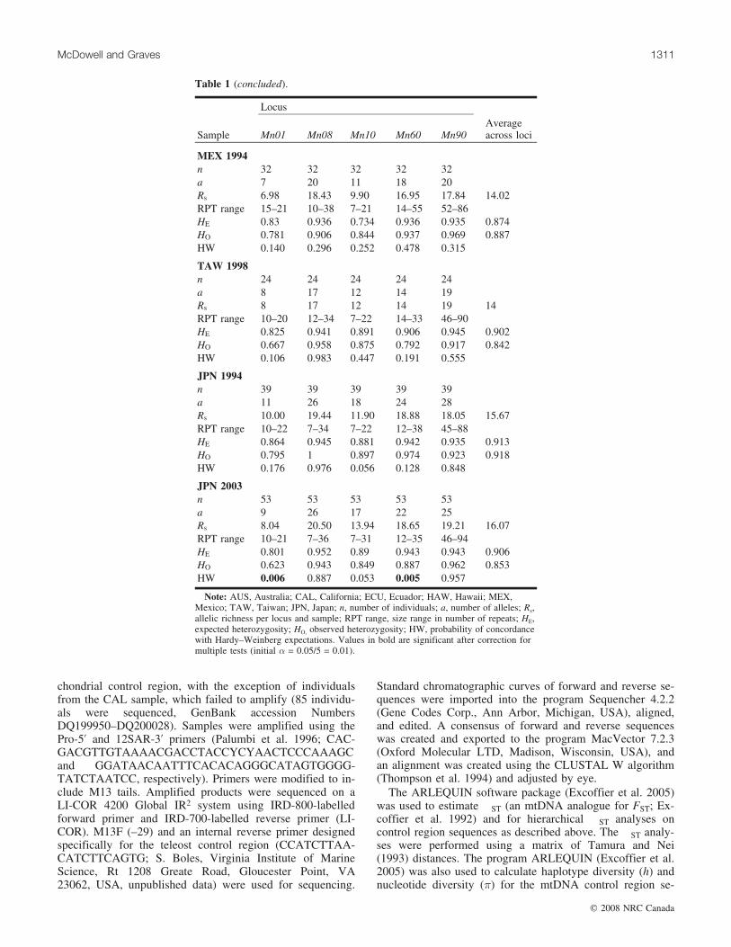
Table 1. Summary statistics for five microsatellite loci among striped marlin(Kajikia audax) samples.

Locus

Sample Mn01 Mn08 Mn10 Mn60 Mn90Averageacross loci

AUS 1994n 37 37 37 37 37a 9 20 12 23 25Rs 7.93 17.25 11.08 19.54 21.50 15.46RPT range 14–22 7–35 7–24 12–38 22–88HE 0.77 0.93 0.89 0.94 0.95 0.896HO 0.78 0.92 0.94 0.95 0.97 0.912HW 0.359 0.323 0.392 0.972 0.979



CAL 2000n 39 39 39 39 39a 9 22 14 23 24Rs 8.60 18.33 12.09 20.51 19.91 15.89RPT range 14–22 10–35 7–22 12–52 22–90HE 0.853 0.937 0.884 0.952 0.938 0.913HO 0.795 0.923 0.897 0.923 0.923 0.982HW 0.326 0.447 0.878 0.550 0.186

ECU 1995n 39 39 39 39 39a 8 22 15 25 22Rs 7.73 18.50 12.44 20.06 18.60 15.46RPT range 14–21 10–38 7–24 14–51 46–90HE 0.775 0.935 0.871 0.941 0.941 0.893HO 0.795 0.949 0.846 0.974 0.974 0.908HW 0.471 0.331 0.004 0.682 0.864

HAW 1998n 48 48 48 48 48a 10 23 14 27 23Rs 8.19 18.84 12.60 20.97 19.00 15.92RPT range 14–39 3–37 7–22 12–53 30–90HE 0.837 0.947 0.891 0.955 0.931 0.745HO 0.75 0.937 0.937 0.875 0.771 0.854HW 0.110 0.325 0.503 0.380 0.186


# 2008 NRC Canada

chondrial control region, with the exception of individualsfrom the CAL sample, which failed to amplify (85 individu-als were sequenced, GenBank accession NumbersDQ199950–DQ200028). Samples were amplified using thePro-5’ and 12SAR-3’ primers (Palumbi et al. 1996; CAC-GACGTTGTAAAACGACCTACCYCYAACTCCCAAAGCand GGATAACAATTTCACACAGGGCATAGTGGGG-TATCTAATCC, respectively). Primers were modified to in-clude M13 tails. Amplified products were sequenced on aLI-COR 4200 Global IR2 system using IRD-800-labelledforward primer and IRD-700-labelled reverse primer (LI-COR). M13F (–29) and an internal reverse primer designedspecifically for the teleost control region (CCATCTTAA-CATCTTCAGTG; S. Boles, Virginia Institute of MarineScience, Rt 1208 Greate Road, Gloucester Point, VA23062, USA, unpublished data) were used for sequencing.

Standard chromatographic curves of forward and reverse se-quences were imported into the program Sequencher 4.2.2(Gene Codes Corp., Ann Arbor, Michigan, USA), aligned,and edited. A consensus of forward and reverse sequenceswas created and exported to the program MacVector 7.2.3(Oxford Molecular LTD, Madison, Wisconsin, USA), andan alignment was created using the CLUSTAL W algorithm(Thompson et al. 1994) and adjusted by eye.

The ARLEQUIN software package (Excoffier et al. 2005)was used to estimate �ST (an mtDNA analogue for FST; Ex-coffier et al. 1992) and for hierarchical �ST analyses oncontrol region sequences as described above. The �ST analy-ses were performed using a matrix of Tamura and Nei(1993) distances. The program ARLEQUIN (Excoffier et al.2005) was also used to calculate haplotype diversity (h) andnucleotide diversity (�) for the mtDNA control region se-

Table 1 (concluded).

Locus

Sample Mn01 Mn08 Mn10 Mn60 Mn90Averageacross loci

MEX 1994n 32 32 32 32 32a 7 20 11 18 20Rs 6.98 18.43 9.90 16.95 17.84 14.02RPT range 15–21 10–38 7–21 14–55 52–86HE 0.83 0.936 0.734 0.936 0.935 0.874HO 0.781 0.906 0.844 0.937 0.969 0.887HW 0.140 0.296 0.252 0.478 0.315

TAW 1998n 24 24 24 24 24a 8 17 12 14 19Rs 8 17 12 14 19 14RPT range 10–20 12–34 7–22 14–33 46–90HE 0.825 0.941 0.891 0.906 0.945 0.902HO 0.667 0.958 0.875 0.792 0.917 0.842HW 0.106 0.983 0.447 0.191 0.555

JPN 1994n 39 39 39 39 39a 11 26 18 24 28Rs 10.00 19.44 11.90 18.88 18.05 15.67RPT range 10–22 7–34 7–22 12–38 45–88HE 0.864 0.945 0.881 0.942 0.935 0.913HO 0.795 1 0.897 0.974 0.923 0.918HW 0.176 0.976 0.056 0.128 0.848

JPN 2003n 53 53 53 53 53a 9 26 17 22 25Rs 8.04 20.50 13.94 18.65 19.21 16.07RPT range 10–21 7–36 7–31 12–35 46–94HE 0.801 0.952 0.89 0.943 0.943 0.906HO 0.623 0.943 0.849 0.887 0.962 0.853HW 0.006 0.887 0.053 0.005 0.957

Note: AUS, Australia; CAL, California; ECU, Ecuador; HAW, Hawaii; MEX,Mexico; TAW, Taiwan; JPN, Japan; n, number of individuals; a, number of alleles; Rs,allelic richness per locus and sample; RPT range, size range in number of repeats; HE,expected heterozygosity; HO, observed heterozygosity; HW, probability of concordancewith Hardy–Weinberg expectations. Values in bold are significant after correction formultiple tests (initial � = 0.05/5 = 0.01).


# 2008 NRC Canada

quence data. PAUP* 4.0 (Swofford 2000) was used to gen-erate the table of variable sites and a neighbor-joining(Saitou and Nei 1987) tree based on the Tamura–Nei dis-tance (Tamura and Nei 1993; Fig. 2). DnaSP 4.0 (Rozas etal. 2003) was used to estimate the nearest-neighbor statistic,Snn (Hudson 2000), for the mtDNA control region sequencesusing 10 000 permutations and gaps excluded in pairwisecomparisons. The Snn statistic measures how often the near-est neighbors in sequence space are from the same localityin geographical space and is particularly appropriate when his large and sample sizes are small (Hudson 2000). Signifi-cance levels were adjusted using the sequential Bonferronitechnique (Rice 1989) in all cases of multiple tests.

Results

Genetic variationFor microsatellite data, the number of alleles per locus

varied from 7 at locus Mn01 to 27 at locus Mn60 (Table 1).Allelic richness per locus and sample ranged from 6.98 atlocus Mn01 in the MEX 1994 sample to 24.16 in theAUS 2005 sample at locus Mn90; the average across lociranged from 14 in TAW 1998 to 16.87 in AUS 2005(Table 1). Average observed heterozygosities ranged from0.67 at locus Mn01 in the AUS 1996 and TAW 1998 sam-ples to 0.97 at the Mn60 (ECU 1995 and JPN 1994) andMn90 (AUS 1994, ECU 1995, MEX 1994) loci; the averageacross loci ranged from 0.84 in TAW 1998 to 0.913 inCAL 2000 (Table 1). Average expected heterozygositiesranged from 0.73 in the MEX 1994 sample at Mn10 to 0.96in the HAW 1998 sample at Mn60 and from 0.74 forHAW 1998 to 0.91 for CAL 2000 and JPN 1994 (Table 1).Three of the 50 tests for conformance to the expectations toHardy–Weinberg equilibrium differed significantly after cor-rections for multiple tests. The ECU 1995 sample had a gen-otypic distribution that differed significantly at Mn10, andthe JPN 2003 sample differed at Mn01 and Mn60 (heterozy-gote deficits; Table 1). Analysis with the MICRO-CHECKER software showed no evidence that null alleles,stuttering, or large allele dropout affected any of the loci,and rescoring of samples confirmed that alleles were beingsized consistently across gels; consequently, all loci wereincluded in all analyses.

Aligned mitochondrial control region sequences rangedfrom 781 to 807 bp, excluding gaps. Overall, 570 characterswere constant, 249 were variable, and 58 insertions–deletionswere observed. Of the 249 variable sites, 162 were parsimonyinformative. For mtDNA, there were 79 haplotypes detectedamong the 83 striped marlin sequenced at the control region,and no haplotype was detected more than twice. Among thefour haplotypes that were shared, one was common to twoJPN samples, one occurred in JPN and TAW, one in JPNand HAW, and one in HAW and MEX (Fig. 2). Haplotypediversity (h) was 0.998 over all samples and ranged from0.98 to 1.0. Nucleotide diversity (p) was 0.044 ± 0.021 overall samples and ranged from 0.039 ± 0021 in the AUS sampleto 0.054 ± 0.029 in the TAW sample.

Population structure based on microsatellitesThe presence of temporal stability of the AUS (1994,

1996, 2005) and JPN (1994, 2003) samples was assessed us-

ing pairwise multilocus FST values (10 000 permutations ofthe data). In addition, an AMOVA was conducted for thethree AUS samples. The FST between the two JPN sampleswas –0.0001 (P = 0.540). FST values for the three Australiansamples ranged from –0.0035 (P = 0.872) betweenAUS 1994 and AUS 2005 to 0.0047 (P = 0.093) betweenAUS 1996 and AUS 2005; no values were significant. AnAMOVA among the AUS collections indicated that only0.12% of the variation was among samples (P = 0.252, Ta-ble 2) while 99.88% was within samples.

To examine whether results of multilocus FST analyseswere being driven by a single locus, population pairwiseFST values were calculated separately for each locus. In pop-ulation pairwise FST comparisons across all loci, 18/21(85.7%) were significant (P < 0.05, data not shown), and re-sults for individual loci ranged from 8/21 (38%) for Mn60 to14/21 (66.7%) for Mn01. The global multilocus FST acrossall samples was 0.013 (P < 0.001), and single locus valuesranged from 0.0336 at Mn01 to 0.0067 at Mn90; all valueswere highly significant (P < 0.001).

Since there was no evidence of temporal variation amongsamples in the microsatellite data, the temporal replicate col-lections were pooled for subsequent analyses. The globalFST among all samples was 0.0134 (P < 0.001). Pairwisemultilocus FST values ranged from 0.0004 (P = 0.435) be-tween CAL and JPN to 0.0276 (P < 0.001) between MEXand AUS; in general, FST values were highest between theMEX sample and all other locations (Table 3). AMOVAswere performed to maximize the amount of variance due tovariation among groups of samples (regions). Since the JPN,HAW, and CAL samples were not significantly different inpairwise comparisons (Table 3), they were grouped togetherfor AMOVA analysis and collectively designated‘‘northern’’ resulting in an FST of 0.002 (P = 0.089). Addi-tion of TAW to the northern sample resulted in an FST of0.004 (P = 0.005), a small but significant difference amongcollections within the group. Grouping samples into strictlynorthern (JPN, TAW, HAW, CAL) and southern (AUS,ECU, MEX) groups revealed small but significant spatialdifferences among regions (FCT = 0.004, P < 0.001).However, grouping samples into strictly east (JPN, TAW,AUS) and west (CAL, MEX, ECU) collections revealed nosignificant spatial differentiation among the samples(FCT = –0.002, P = 0.696). Differences among regions (%variation and fixation index) were maximized and variationwithin regions was minimized when the northern collectionwas grouped and all remaining collections (AUS, MEX,ECU) were held separately (FCT = 0.014, P < 0.0001).Likewise, the PCA analysis (Fig. 3) indicated that theJPN, TAW, CAL, and HAW composed a single (northern)group, while the AUS, MEX, and ECU collections ap-peared to represent distinct groups. The two principal axestogether explained 50.67% of the total genetic diversity.The first principal component explained 29.81% (P < 0.001)of the variance among the populations, and the second axisaccounted for 20.86% of the variance (P < 0.001). Thethird component accounted for 11.84% of the variance andwas not significant (P = 0.989).

Population structure based on mtDNAUnlike results from the microsatellite markers, there were


# 2008 NRC Canada

no significant pairwise comparisons of �ST based onTamura–Nei distances (Tamura and Nei 1993). Valuesranged from –0.0587 between HAW and TAW to 0.0430between ECU and AUS. However, the nearest-neighbor sta-tistic (Snn) revealed a significant, nonrandom association be-

tween mtDNA sequence similarity and geographic location(Snn = 0.202, P < 0.0001). An AMOVA indicated that popu-lation divisions were essentially the same as those obtainedfrom microsatellite data. Grouping the JPN, TAW, andHAW collections into the northern group and holding all

Fig. 2. Neighbour-joining tree of striped marlin (Kajikia audax) mitochondrial control region sequences (819 bp) based on the Tamura andNei (1993) distances. Sample designations are as follows: Japan, Jpn; Taiwan, Taw; Australia, Aus; Hawaii, Haw; California, Cal; Mexico,Mex; and Ecuador, Ecu.


# 2008 NRC Canada

other samples separate resulted in a �CT = 0.034 (P <0.0001; Table 4).

Migration and effective population sizeThe average Q values estimated with the MIGRATE soft-

ware for the microsatellite data set ranged from 0.2923(SE = 0.0277) in AUS to 1.0512 (SE = 0.1258) in JPN(Fig. 4). The estimates of per generation immigration rateswere also variable among samples (only values >20 areshown in Fig. 4 to facilitate presentation of data). Analysisof the historical migration rate (M) indicates that gene flowhas historically been asymmetrical, and JPN has been themost important contributor to gene flow. For JPN, TAW,and ECU, mutation has likely been more important thangene flow for introducing variation into the population,while gene flow appears to have been more important forbringing new alleles into MEX and CAL. Interestingly,AUS appears to have received immigrants from the North

Pacific, but has been an important source of immigrants forCAL and MEX in the eastern Pacific.

Discussion

Stock structureThe results of the AMOVA and PCA analyses clearly

delineate the presence of at least four genetically discretegroups of striped marlin within the Pacific Ocean, whichcorrespond to the four described striped marlin spawningareas. As with previous genetic studies, our results show ge-netic homogeneity between temporal replicates, indicatingthat the observed genetic heterogeneity among samplesfrom different locations reflects geographical differences inthe genetic structure rather than sampling error. For the mi-crosatellite data, a locus-by-locus analysis shows that the ob-served structure was not driven by any single locus or pairof loci (data not shown). These results are corroborated by

Table 2. Analysis of molecular variance (AMOVA) among regions and locations for striped marlin (Kajikia audax) based on thenumber of alleles (FST) for microsatellite data.

Source of variation (FST) % variationFixationindex P

SamplesAll samples Among samples 1.35 0.013 <0.0001

Within samples 98.65Temporal stability Among samples 0.12 0.001 0.252

(AUS 1994, 1996, 2005) Within samples 99.88Temporal stability Among samples –0.01 0.000 0.543

(JPN 1994, 2003) Within samples 100.01North Among samples 0.20 0.002 0.089

(JPN, HAW, CAL) Within samples 99.80North Among samples 0.40 0.004 0.005

(JPN, TAW, HAW, CAL) Within samples 99.60South Among samples 2.03 0.020 <0.0001

(AUS, ECU, MEX) Within samples 97.97South Among samples 2.13 0.021 <0.0001

(AUS, ECU, MEX, TAW) Within samples 97.87North and South Among regions 0.50 0.004 <0.0001

(North: HAW, JPN, TAW, CAL; Among populations and regions 1.05 0.011 <0.0001South: AUS, ECU, MEX) Within populations 98.45 0.015 <0.0001

North and South Among regions 0.22 0.002 0.210(North: HAW, JPN, CAL; Among populations and regions 1.22 0.012 <0.0001South: AUS, ECU, MEX, TAW) Within populations 98.56 0.014 <0.0001

East and West Among regions –0.15 –0.002 0.696(East: JPN, TAW, AUS; Among populations and regions 1.6 0.016 <0.0001West: CAL, MEX, ECU) Within populations 98.55 0.014 <0.0001

RegionsNorth; Southwest; Southeast Among regions 0.70 0.007 0.008

(North: JPN, HAW; Southwest: AUS, TAW; Among populations and regions 0.82 0.008 <0.0001Southeast: MEX, ECU) Within populations 98.48 0.152 <0.0001

North; MEX; ECU; (AUS, TAW) Among regions 0.75 0.008 0.038(North: JPN, HAW, CAL) Among populations and regions 0.76 0.008 <0.0001

Within populations 98.48 0.015 <0.0001North; MEX; ECU; AUS Among regions 1.28 0.012 <0.0001

(North: JPN, HAW, CAL, TAW) Among populations and regions 0.40 0.004 <0.0001Within populations 98.32 0.017 <0.0001

Note: Significance was assessed using 10 100 permutations. See Table 1 for location abbreviations.


# 2008 NRC Canada

our observation of population structure based on data fromthe mtDNA locus and suggest the presence of a minimumof four long-term, temporally stable genetic stocks of stripedmarlin in the Pacific Ocean.

In the southwest Pacific, our temporal samples spanning11 years off Port Stephens, Australia, suggest that geneticvariation in striped marlin is temporally stable, at least inthis area. Pairwise comparisons of the AUS collection withother all collections were highly significant, and the AUScollections were clearly separated from the other collectionsin the PCA analysis. These results are consistent with otherfisheries data. Striped marlin are known to spawn off easternAustralia based on the presence of larvae. In addition, tag-ging data shows that the majority of striped marlin releasedoff Australia are recaptured within several hundred nauticalmiles (1 n.m. = 1.852 km) of release even after 6–9 monthsat liberty and have a mean displacement of 200 n.m., sug-gesting that striped marlin in this area are residential (Ortizet al. 2003). Additionally, no tag–recaptures of marlin re-leased in the southwest Pacific have been recorded in theeastern Pacific or vice versa (Ortiz et al. 2003).

Like the southwest Pacific, the ECU collection in thesoutheast Pacific was significantly different from all othersamples based on microsatellite data. Pairwise FST compari-sons between ECU and other samples were all significant,and as with previous studies (Graves and McDowell 1994),ECU was distinct from the eastern Pacific (MEX) collection.Tagging studies have indicated that movements in the south-east Pacific are complex, but that there is a general move-ment towards the Galapagos and southern Central Americancoastline, which then expands offshore and southwest inOctober–March. This has been correlated to the migrationof mature individuals towards the spawning grounds (Kumeand Joseph 1969), as over 75% of fish caught in this area atthis time are mature, and supports the lack of mixing indi-cated by genetic data.

Several lines of evidence support the genetic clustering ofthe northern striped marlin samples (JPN, HAW, TAW, andCAL). The striped marlin has a continuous horseshoe-shaped distribution with one arm that extends across theNorth Pacific. Tag–recapture data have shown movementsinto the area around Hawaii by predominantly 40–60 kgstriped marlin migrating from Californian coastal watersfrom late autumn – early winter. However, there have beenno California recaptures of striped marlin tagged in Hawaii(Ortiz et al. 2003), nor are fish in spawning condition caughtoff the coast of California. Whether there is movement be-tween the central North Pacific (HAW) and western Pacific(JPN, TAW) is unknown because there has been negligibletagging effort in the northeast Pacific. However, althoughstriped marlin spawn in the region southeast of Japan(Squire and Suzuki 1990), few juveniles are caught in thisarea and it has been suggested that they may migrate fromthis region, returning when they become mature (Bromheadet al. 2004). This supposition is supported by the fact thatjuvenile striped marlin appear in the central North Pacific ataround 10 kg, and neither larger fish nor larvae are found inthis area, suggesting that juveniles use the central NorthPacific as a feeding ground (Matsumoto and Kazama 1974).Taken together, these data imply that juvenile striped marlinspawned off Japan may be moving east into the centralT

able

3.M

atri

xof

pair

wis

eF

STva

lues

base

don

mic

rosa

telli

teda

ta(b

elow

diag

onal

)an

dpa

irw

ise�

STva

lues

for

mtD

NA

sequ

ence

sba

sed

onth

eT

amur

a–N

eidi

stan

ce(T

amur

aan

dN

ei19

93)

(abo

vedi

agon

al).

AU

SC

AL

EC

UH

AW

ME

XT

AW

JPN

AU

S—

NA

0.04

30(0

.775

)0.

0184

(0.2

10)

0.01

43(0

.245

)0.

0045

(0.3

24)

0.01

67(0

.200

)C

AL

0.01

56(<

0.00

1)—

NA

NA

NA

NA

NA

EC

U0.

0174

(<0.

001)

0.01

04(<

0.00

1)—

–0.0

300

(0.7

75)

–0.0

130

(0.5

98)

–0.2

740

(0.6

88)

0.01

86(0

.199

)H

AW

0.01

04(<

0.00

1)0.

0028

(0.1

31)

0.01

45(<

0.00

1)—

0.02

25(0

.431

)–0

.058

7(0

.950

)0.

0003

(0.4

03)

ME

X0.

0276

(<0.

001)

0.02

32(<

0.00

1)0.

0114

(0.0

02)

0.02

24(<

0.00

1)—

–0.0

320

(0.6

99)

0.02

60(0

.151

)T

AW

0.02

31(<

0.00

1)0.

0082

(0.0

25)

0.01

87(<

0.00

1)0.

0118

(0.0

02)

0.02

74(<

0.00

1)—

–0.0

424

(0.1

51)

JPN

0.01

65(<

0.00

1)0.

0004

(0.4

35)

0.01

00(<

0.00

1)0.

0030

(0.0

52)

0.01

52(<

0.00

1)0.

0068

(0.0

20)

—

Not

e:Si

gnif

ican

ceva

lues

(in

pare

nthe

ses)

are

base

don

1000

0pe

rmut

atio

ns.

NA

,no

tav

aila

ble.

See

Tab

le1

for

loca

tion

abbr

evia

tion

s.


# 2008 NRC Canada

Pacific to feed and that some of these fish may end up offthe coast of California before returning to the spawninggrounds off Japan.

Although the TAW samples grouped most closely withthe other northern samples and no significant �ST differen-ces were noted between TAW and other northern samplesbased on mtDNA data, microsatellite data revealed smallbut significant pairwise differences between TAW and CALand between TAW and JPN. Striped marlin larvae have

been found in the eastern Indian Ocean off the northwestcoast of Australia (Nakamura 1983) as well as in the Timorand Banda seas (Ueyanagi and Wares 1975). Derivation ofthe TAW samples from a mixture of both the Indian Oceanand western North Pacific spawning stocks is one possibleexplanation for the observed differences, and the relation-ship between Pacific Ocean and Indian Ocean striped marlinshould be examined further in future studies.

One of the most interesting results of the current study is

Table 4. Analysis of molecular variance (AMOVA) among regions and locations for striped marlin (Kajikia audax)collections based on mtDNA data.

Source of variation (�ST) % variationFixationindex P

All samples Among samples –0.67 –0.007 0.642Within samples 100.67 — —

(JPN, TAW, HAW); (MEX, ECU); AUS Among regions 3.14 0.031 <0.0001Among populations and regions –2.77 –0.029 0.710Within populations 99.63 0.004 0.623

(JPN, HAW, TAW); MEX; ECU; AUS Among regions 3.40 0.034 <0.0001Among populations and regions –3.12 –0.032 0.377Within populations 99.71 0.003 0.633

(JPN, TAW); MEX; ECU; AUS; HAW Among regions 4.31 0.043 <0.0001Among populations and regions –4.39 –0.046 0.286Within populations 100.08 –0.001 0.637

(JPN, TAW); (MEX, ECU); AUS; HAW Among regions 3.47 0.035 0.005Among populations and regions — –3.49 –0.036Within populations 100.02 –0.000 0.632

Note: �ST was calculated based on Tamura–Nei distance (Tamura and Nei 1993). Significance was assessed using 10 100 permu-tations. The two years of JPN data were held separately in this analysis, although they are represented as a single year below. SeeTable 1 for location abbreviations.

Fig. 3. Principal component analysis (PCA) showing the genetic relationship among striped marlin (Kajikia audax). PCA axis 1 explains29.81% of the variance; axis 2 explains 20.86% of the variance. Circles are drawn around groups of collections based on results of pairwiseFST values; nonsignificant comparisons are grouped.


# 2008 NRC Canada

the presence of statistically significant differences betweenstriped marlin taken off California (CAL) and those takenoff Baja California (MEX), despite the fact that taggingstudies clearly demonstrate migration between these areas.Movements of Mexican fish northward towards Californiaduring the summer months have been documented (e.g., Ar-mas et al. 1999), and most tagged southern California fishare recaptured off Baja California (Ortiz et al. 2003). In ad-dition, longline data show that fluctuations in catch rates inthe Baja California region are correlated with fluctuations inthe rest of the eastern Pacific, suggesting considerable mix-ing within this area (Squire and Au 1990). Although our re-sults could be due to sampling error associated withinsufficient sample size, there are data to support our find-ing. In the Northeast Pacific off Baja California, 65% offish caught are mature (Squire and Suzuki 1990), while nofish in spawning condition are caught off the coast of Cali-fornia (M. Hinton, Inter-American Tropical Tuna Commis-sion, 8604 La Jolla Shores Drive, La Jolla, California,personal communication, 2006). In addition, most stripedmarlin recaptured off Baja California are caught within afew hundred nautical miles of release even after nearly2 years at liberty (Ortiz et al. 2003). Perhaps the most con-

vincing support for validity of results suggesting that theMEX and CAL collections are representative of distinctpopulations is based on data from satellite tagging. Since2000, 115 satellite tags have been put on striped marlinnear Magdelena Bay, Baja California, Mexico. Althoughthey have been tracked for up to 9 months (November–July), none have been found to range from Mexican waters(M. Domeier, Pfleger Institute of Environmental Research,Oceanside, California, personal communication). Takentogether, the available data suggest the presence of a self-sustaining resident population of striped marlin off the coastof Mexico. Since it is thought that striped marlin off thecoast of California are composed of subadult fish that arethought to travel to spawning grounds in the western Pacificupon maturity, it seems plausible that striped marlin fromboth stocks mix on offshore feeding grounds. This mixingcould explain the apparent conflict between the genetic andconventional tagging data. Other large pelagic species, mostnotably the bluefin tuna (Thunnus thynnus), have recentlybeen shown to mix on feeding grounds but maintain distinctstocks driven by spawning site fidelity (Carlsson et al.2006).

Microsatellite data are capable of detecting small genetic

Fig. 4. Historical effective population size (Q) and migration rate scaled by mutation (M) between populations, including the standard errorsacross the five runs using the program MIGRATE (Beerli and Felsenstein 2001). Values of M less than 20 are not shown. See Table 1 forlocation abbreviations.


# 2008 NRC Canada

differences between populations because of their high muta-tion rate. This has led to the realization that statistically sig-nificant differences between populations do not alwaysindicate biologically significant differences (Waples 1998;Hedrick 1999). However, the results of this study correlatewell with the other fishery data; the seemingly cyclicalmovements of adults with season combined with the pres-ence of distinct spawning grounds. In addition, just over60% of global recaptures of tagged striped marlin occurwithin 200 n.m. of the release point, and 84% occur within500 n.m., while less than 8% are recaptured over 1000 n.m.from the point of release, indicating at least some level ofregional fidelity (Ortiz et al. 2003; Bromhead et al. 2004).There are also morphological differences between northernand southern Pacific striped marlin; southern fish are largerthan northern fish and there are differences in pectoral finlength (Ueyanagi and Wares 1975). Finally, analysis oflongline data has shown that catch rates of striped marlinnear the equator in the western Pacific are exceptionallylow, which further implies the potential for separate north-ern and southern stocks particularly in the west (Ueyanagiand Wares 1975).

Historical migration and effective population sizeExamination of the asymmetric matrix of historical migra-

tion rates and relative effective population size estimatessuggest historical patterns that are not apparent using tradi-tional genetic analyses. Although no genetic differentiationwas noted among TAW, JPN, HAW, and CAL, estimates oflong-term effective population sizes (Q) in these samplesranged from 1.05 to 0. 37. This discrepancy may resultfrom sampling different components of the population inthe different areas; mature fish are not found in HAW orCAL, and the effective population sizes in these areas mayappear smaller owing to the exclusion of some age classes.Alternately, striped marlin may have arisen in the westernPacific and subsequently spread eastward to HAW andCAL, although this might be expected to result in fewer al-leles per locus in the HAW and CAL samples, which wasnot evident in this study. Finally, the larger effective popula-tion sizes of the JPN and TAW samples may be due to im-migration from other (Indian Ocean) source populations notincluded in this study, and the more immigrants from theunknown populations that are arriving in the sample popula-tions, the more inflated the estimated population sizes(Beerli 2004).

Interestingly, estimates of Q suggest that the relativelong-term inbreeding effective population size of the CALand MEX samples are nearly identical (0.377 vs. 0.337, re-spectively) and that of all pairwise comparisons, these twosamples have historically had the largest exchange of mi-grants between them (71 and 43, respectively), suggestingthat they comprise two samples from a single population.This corroborates the observed movements of fish betweenthe two areas seen in tagging studies (Armas et al. 1999; Or-tiz et al. 2003) but is contrary to the results of both the sat-ellite tagging data (M. Domeier, Pfleger Institute ofEnvironmental Research, Oceanside, California, personalcommunication) and the finding that these samples are ge-netically distinct. The discrepancy between the high level ofhistorical exchange and an apparent lack of contemporane-

ous gene flow is intriguing. If a subset of the samples takenfrom each location actually belonged to the other stock(some samples were taken at a time and place when stockswere mixed on feeding grounds), the apparent high level ofhistorical migration could simply be an artifact and thisseems the most likely scenario. This highlights the need forfurther study of population structure in striped marlin, assamples used in this study were taken from adult specimensof unknown natal origin rather from juveniles. Recent stud-ies of bluefin tuna (Carlsson et al. 2004) and loggerhead tur-tles, Caretta caretta, (Bowen et al. 2005) have demonstratedthat fine-scale population structure may not be fully eluci-dated by examination of a single life-history stage, andpopulation structure may in fact be obscured by impropersampling.

Results of our study suggest that striped marlin comprisesmultiple genetic stocks. Northern collections of striped mar-lin taken from Japan, Taiwan, Hawaii, and California appearto constitute a single genetic stock, while southern collec-tions from Australia, Mexico, and Ecuador are statisticallysignificantly different from each other as well as from thenorthern samples. These genetic stocks correspond wellwith the known distribution of larvae and provide supportfor the idea that striped marlin either exhibit spawning sitefidelity and (or) are less migratory than other billfishes. Fu-ture studies of striped marlin should include more collectionlocations as well as more temporal replicates and surveys atspawning grounds, as they may reveal the presence of addi-tional genetic stock structure. The presence of geneticallyindependent stocks should be factored into management andconservation decisions impacting striped marlin.

AcknowledgementsWe thank Michael Hinton and Jens Carlsson for helpful

comments and suggestions. We also thank Sandra Boles andJeanette Carlsson for technical assistance. We are indebtedto Ed Everett, Julian Pepperell, Narishito Chow, Dave Holts,and the staff of the Hotel Spa Buenavista for providing sam-ples. This study was supported by grants from NOAA–NMFS and is Virginia Institute of Marine Science, Collegeof William and Mary Contribution No. 2934.

ReferencesArmas, R.G., Sosa-Nishizaki, O., Rodriguez, R.F., and Perez,

V.A.L. 1999. Confirmation of the spawning area of the stripedmarlin, Tetrapturus audax, in the so-called core area of theeastern tropical Pacific off Mexico. Fish. Oceanogr. 8: 238–242.doi:10.1046/j.1365-2419.1999.00102.x.

Beerli, P. 2002. MIGRATE-N: estimation of population sizes andgene flow using the coalescent. Available from popgen.scs.fsu.edu/Migrate-n.html [accessed 8 May 2008].

Beerli, P. 2004. Effect of unsampled populations on the estimationof population sizes and migration rates between sampled popula-tions. Mol. Ecol. 13: 827–836. doi:10.1111/j.1365-294X.2004.02101.x. PMID:15012758.

Beerli, P., and Felsenstein, J. 2001. Maximum likelihood estimationof a migration matrix and effective population sizes in n sub-populations by using a coalescent approach. Proc. Natl. Acad.Sci. U.S.A. 98: 4563–4568. doi:10.1073/pnas.081068098. PMID:11287657.

Bowen, B.W., Bass, A.L., Soares, L., and Toonen, R.J. 2005. Con-


# 2008 NRC Canada

servation implications of complex population structure: lessonsfrom the loggerhead turtle Caretta caretta. Mol. Ecol. 14:2389–2402. doi:10.1111/j.1365-294X.2005.02598.x. PMID:15969722.

Bromhead, D., Pepperell, J., Wise, B., and Findlay, J. 2004. Stripedmarlin: biology and fisheries. Bureau of Rural Science, Can-berra. ISBN:0642475938.

Buonaccorsi, V.P., and Graves, J.E. 2000. Isolation and characteri-zation of novel polymorphic tetra-nucleotide microsatellite mar-kers from the blue marlin, Makaira nigricans. Mol. Ecol. 9:820–821. doi:10.1046/j.1365-294x.2000.00915-2.x. PMID:10849299.

Buonaccorsi, V.P., Morgan, L., Reece, K.S., and Graves, J.E. 1999.Geographic distribution of molecular variance within blue mar-lin Makaira nigricans: a hierarchical analysis of allozyme, sin-gle copy nuclear DNA, and mitochondrial DNA markers.Evolution, 53: 568–579. doi:10.2307/2640793.

Buonaccorsi, V.P., McDowell, J., and Graves, J.E. 2001. Reconcil-ing patterns of inter-ocean molecular variance from four classesof molecular markers in blue marlin Makaira nigricans. Mol.Ecol. 10: 1179–1196. doi:10.1046/j.1365-294X.2001.01270.x.PMID:11380876.

Carlsson, J., McDowell, J.R., Diaz-Jaimes, P., Carlsson, J.E.L.,Boles, S.B., Gold, J.R., and Graves, J.E. 2004. Microsatelliteand mitochondrial DNA analyses of Atlantic bluefin tuna(Thunnus thynnus thynnus) population structure in the Mediter-ranean Sea. Mol. Ecol. 13: 3345–3356. doi:10.1111/j.1365-294X.2004.02336.x. PMID:15487994.

Carlsson, J., McDowell, J.R., Carlsson, J.E.L., and Graves, J.E.2006. Genetic identity of YOY bluefin tuna from eastern andwestern Atlantic spawning areas. J. Hered. 98: 23–28. doi:10.1093/jhered/esl046. PMID:17158466.

Estoup, A., Largiader, C.R., Perrot, E., and Chourrout, D. 1996.Rapid one-tube DNA extraction for reliable PCR detection offish polymorphic markers and transgenes. Mol. Mar. Biol. Bio-technol. 5: 295–298.

Excoffier, L., Smouse, P.E., and Quattro, J.M. 1992. Analysis ofmolecular variance inferred from metric distances among DNAhaplotypes: application of human mitochondrial DNA restrictiondata. Genetics, 147: 915–925.

Excoffier, L., Laval, G., and Schneider, S. 2005. Arlequin ver. 3.0:An integrated software package for population genetics dataanalysis. Evol. Bioinf. Online, 1: 47–50.

Falterman, B.J. 1999. Indo-Pacific population structure of the blackmarlin, Makaira indica, inferred from molecular markers. M.Sc.thesis, Department of Fisheries Science, Virginia Institute ofMarine Science, School of Marine Science, College of Williamand Mary, Gloucester Point, Va.

Finnerty, J.K., and Block, B.A. 1992. Direct sequencing ofmitochondrial DNA detects highly divergent haplotypes in bluemarlin (Makaira nigricans). Mol. Mar. Biol. Biotechnol. 1: 200–211.

Goudet, J. 1995. FSTAT (version 1.2): a computer program to cal-culate F-statistics. J. Hered. 86: 485–486.

Guo, S.W., and Thompson, E.A. 1992. Performing the exact-testfor Hardy–Weinburg proportion for multiple alleles. Biometrics,48: 361–372. doi:10.2307/2532296. PMID:1637966.

Graves, J.E. 1998. Molecular insights into the population structuresof cosmopolitan marine fishes. J. Hered. 89: 427–437. doi:10.1093/jhered/89.5.427.

Graves, J.E., and McDowell, J.R. 1994. Genetic analysis of stripedmarlin (Tetrapturus audax) population structure in the PacificOcean. Can. J. Fish. Aquat. Sci. 51: 1762–1768. doi:10.1139/f94-177.

Graves, J.E., and McDowell, J.R. 1995. Inter-ocean genetic diver-gence of istiophorid billfishes. Mar. Biol. (Berl.), 122: 193–204.

Graves, J.E., and McDowell, J.R. 2001. A genetic perspective onthe stock structures of blue marlin and white marlin in theAtlantic Ocean. Coll. Vol. Sci. Papers. ICCAT, 53: 180–187.

Graves, J.E., and McDowell, J.R. 2003. Population structure of theworld’s istiophorid billfishes: a genetic perspective. Mar.Freshw. Res. 54: 287–298. doi:10.1071/MF01290.

Graves, J.E., and McDowell, J.R. 2006. Genetic analysis of whitemarlin (Tetrapturus albidus) stock structure. Bull. Mar. Sci. 79:469–482.

Hedrick, P.W. 1999. Highly variable genetic loci and their interpre-tation in evolution and conservation. Evolution, 53: 313–318.doi:10.2307/2640768.

Hinton, M.G., and Maunder, M.N. 2003. Status of striped marlin inthe eastern Pacific Ocean in 2002 and outlook for 2003–2004.Report 4. Inter-American Tropical Tuna Commission, La Jolla,Calif.

Hudson, R.R. 2000. A new statistic of detecting genetic differentia-tion. Genetics, 155: 2001–2014.

King, D.M. 1990. Economic trends affecting commercial billfishfisheries In Planning the Future of Billfishes. Research andManagement in the 90’s and Beyond. Proceedings of the 2ndInternational Billfish Symposium, Kailua–Kona, Hawaii, 1–5 August 1988. Part 2. Edited by R.H. Stroud. NationalCoalition for Marine Conservation, Leesburg, Va. pp. 89–102.

Kume, S., and Joseph, J. 1969. Size composition and sexualmaturity of billfish caught by the Japanese longline fishery inthe Pacific Ocean east of 130W. Bull. Far Seas Fish. Res. Lab.2: 115–162.

Matsumoto, W.M., and Kazama, T.K. 1974. Occurrence of youngbillfishes in the Central Pacific Ocean. In Proceedings of theInternational Billfish Symposium Kailua–Kona, Hawaii, 9–12 August 1972. Part 2. Edited by R.S. Shomura and F. Wil-liams. National Marine Fisheries, Service, Seattle, Wash.NOAA Tech. Rep. NMFS SSRF-675. pp. 238–247.

Morgan, L.W. 1992 Allozyme analysis of billfish population struc-ture. M.Sc. thesis, Department of Fisheries Science, Virginia In-stitute of Marine Science, School of Marine Science, College ofWilliam and Mary, Gloucester Point, Va.

Nakamura, I. 1983. Systematics of billfishes (Xiphiidae and Istio-phoridae). Publ. Seto Mar. Biol. Lab. 28: 255–396.

Nakamura, I. 1985. FAO species catalogue. Vol. 5. Billfishes of theworld. An annotated and illustrated catalogue of marlins, sail-fishes, spearfishes and swordfishes known to date. FAO Fish-eries Synopses 125, Rome, Italy.

Ortiz, M., Prince, E.D., Serafy, J.E., Holts, D.B., Davy, K.B.,Pepperell, J.G., Lowry, M.B., and Holdsworth, J.C. 2003. Aglobal overview of the major constituent-based billfish taggingprograms and their results since 1954. Mar. Freshw. Res. 54:489–507. doi:10.1071/MF02028.

Palumbi, S.R., Martin, A., and Romano, S. McMillan, W.O., Stice,L., and Grabowski, G. 1996. The simple fool’s guide to PCR.Kewalo Marine Laboratory and University of Hawaii, Honolulu,Hawaii.

Penrith, M.J., and Cram, D.L. 1974. The Cape of Good Hope: ahidden barrier to billfishes. In Proceedings of the InternationalBillfish Symposium Kailua–Kona, Hawaii, 9–12 August 1972.Part 2. Edited by R.S. Shomura and F. Williams. National Mar-ine Fisheries Service, Seattle, Wash. NOAA Tech. Rep. NMFSSSRF-675. pp. 175–187.

Raymond, M., and Rousset, F. 1995. GENEPOP (version 1.2)population genetics software for exact test and ecumenicism. J.Hered. 86: 248–249.


# 2008 NRC Canada

Rice, W.R. 1989. Analyzing tables of statistical tests. Evolution,43: 223–225. doi:10.2307/2409177.

Rozas, J., Sanchez-DelBarrio, J.C., Messeguer, X., and Rozas, R.2003. DnaSP, DNA polymorphism analyses by the coalescentand other methods. Bioinformatics, 19: 2496–2497. doi:10.1093/bioinformatics/btg359. PMID:14668244.

Saitou, N., and Nei, M. 1987. The neighbor-joining method: a newmethod for reconstructing phylogenetic trees. Mol. Biol. Evol. 4:406–425. PMID:3447015.

Sambrook, J., and Russell, D.W. 2001. Molecular cloning: a la-boratory manual. 3rd ed. Cold Spring Harbor Laboratory Press,Cold Spring Harbor, N.Y.

Seutin, G., White, B.N., and Boag, P.T. 1991. Preservation of avianblood and tissue samples for DNA analysis. Can. J. Zool. 69:82–90. doi:10.1139/z91-013 .

Skillman, R.A. 1990. Stock identification and billfish management.In Planning the Future of Billfishes: Research and Managementin the 90’s and Beyond. Proceedings of the 2nd InternationalBillfish Symposium, Kailua–Kona, Hawaii, 1–5 August 1988.Part 2. Edited by R.H. Stroud. National Coalition for MarineConservation, Leesburg, Va. pp. 207–213.

Smedbol, R.K., McPerson, A., Hansen, M.M., and Kenchington, E.2002. Myths and moderation in marine ‘metapopulations’? FishFish. Ser. 3: 20–35.

Squire, J.L., and Au, D.K.W. 1990. Striped marlin in the north-eastPacific — a case for local depletrion and core area management.In Planning the Future of Billfishes: Research and Managementin the 90’s and Beyond. Proceedings of the 2nd InternationalBillfish Symposium, Kailua–Kona, Hawaii, 1–5 August 1988.Part 2. Edited by R.H. Stroud. National Coalition for MarineConservation, Leesburg, Va. pp. 199–214.

Squire, J.L., Jr., and Suzuki, Z. 1990. Migration trends of stripedmarlin (Tetrapturus audax) in the Pacific Ocean. In Planningthe Future of Billfishes: Research and Management in the90’s and Beyond. Proceedings of the 2nd International Billfish

Symposium, Kailua–Kona, Hawaii, 1–5 August 1988. Part 2.Edited by R.H. Stroud. National Coalition for Marine Conser-vation, Leesburg, Va. pp. 67–80.

Swofford, D.L. 2000. PAUP*. Phylogenetic analysis using parsi-mony (*and other methods). Version 4. Sinauer Associates, Sun-derland, Mass.

Talbot, F.H., and Penrith, M.J. 1962. Tunnies and marlins of SouthAfrica. Nature (London), 193: 558–559. doi:10.1038/193558a0.

Tamura, K., and Nei, M. 1993. Estimation of the number of nu-cleotide substitutions in the control region of mitochondrialDNA in humans and chimpanzees. Mol. Biol. Evol. 10: 512–526. PMID:8336541.

Thompson, J.D., Higgins, D.G., and Gibson, T.J. 1994. CLUSTALW: improving the sensitivity of progressive multiple sequencealignment through sequence weighting, position-specific gappenalties and weight matrix choice. Nucleic Acids Res. 22:4673–4680. doi:10.1093/nar/22.22.4673. PMID:7984417.

Ueyanagi, S., and Wares, P.G. 1975. Synopsis of biological data onstriped marlin, Tetrapturus audax (Philippi, 1887). In Proceed-ings of the International Billfish Symposium, Kailua–Kona,Hawaii, 9–12 August 1972, Part 3. Species synopses. Edited byR.S. Shomura and F. Williams. National Marine Fisheries, Ser-vice, Seattle, Wash. NOAA Tech. Rep. NMFS SSRF-675.pp. 132–159.

van Oosterhout, C., Hutchinson, W.F., Wills, D.P.M., and Shipley,P. 2004. MICRO-CHECKER: software for identifying and cor-recting genotyping errors in microsatellite data. Mol. Ecol.Notes, 4: 535–538. doi:10.1111/j.1471-8286.2004.00684.x.

Waples, R.S. 1998. Separating wheat from the chaff: patterns ofgenetic differentiation in high gene flow species. J. Hered. 89:438–450. doi:10.1093/jhered/89.5.438.

Weir, B.S., and Cockerham, C.C. 1984. Estimating F-statistics forthe analysis of population structure. Evolution, 38: 1358–1370.doi:10.2307/2408641.


# 2008 NRC Canada

population structure of striped marlin kajikia audax) in ...appraise the presence of distinct stocks...

Documents