population pharmacokinetic and pharmacodynamic modelling
TRANSCRIPT

Population Pharmacokinetic and Pharmacodynamic Modelling to Describe the
Effects of APAP Overdose on Novel Biomarkers in UK Patients
Thesis submitted in accordance with the requirements of the University of Liverpool for the
degree of Doctor in Philosophy
By
Areej Turkistani
September 2018
ii
Abstract
Paracetamol (APAP) overdose is a major medical problem in the UK and the leading cause of
drug-induced liver injury (DILI) and acute liver failure. It is involved in 48% of poisoning
admissions to hospital resulting in at least 200 deaths per year. Stratification of risk and the use
of N-acetyl-cysteine (NAC) antidote therapy is sub-optimal and based on a timed determination
of plasma APAP concentration. The current assessment of drug-induced liver injury or
dysfunction in clinical practice is through liver function tests (LFT) obtained from a blood
sample. These tests include serum concentration of total bilirubin (TBL), activity assessment
of liver enzymes (alkaline phosphatase (ALP), aspartate aminotransferase (AST), alanine
aminotransferase (ALT)) and coagulation profile. However, the change in these enzymes’
activity is not specific to DILI and changes are confounded with different diseases of the liver
such as viral hepatitis, fatty liver disease and liver cancer.
Novel mechanistic biomarkers have been demonstrated to provide added value for the early
prediction of APAP-induced hepatotoxicity. These biomarkers are more specific to activity
within the liver, such as Glutamate Dehydrogenase (GLDH) which reflects mitochondrial
dysfunction, Keratin-18 (K18) as a monitor for apoptotic-necrotic dynamics, high mobility
group box-1 (HMGB1) that increases as a result of immune inflammatory system activation
and lastly, serum microRNA (miR-122), which is a highly liver-specific mRNA.
The primary objective of this thesis is to translate these novel biomarkers from mouse animal
models into human models, and then to assess their potential use in clinical practice via
simulation, examining the sensitivity of these biomarkers and their effectiveness in detecting
liver injury. Population Pharmacokinetic and Pharmacodynamic (Pop-PKPD) modelling of the
available data can enable greater understanding of APAP-induced liver injury and newly
identified biomarkers, and was applied to estimate mean population PK parameters of APAP
and PD parameters of each biomarker, taking into account inter and intra subject variability.
The final population PK model for APAP following overdose is a one-compartment disposition
model with first-order absorption, with an exponential residual error model, and alcoholism as
a categorical covariate on CL, with alcoholic patients having a 14% increase in APAP clearance
compared to non-alcoholic patients. The sequential combined effect compartment/indirect
response model for PKPD models was implemented to describe the time course effect of APAP
overdose on current and novel biomarkers. In the BIOPAR study, measured biomarker levels

iii
in most patients tended to fall within normal ranges, with time-courses relatively flat in shape,
and the PKPD models yielded parameter estimates reflecting these trends in the data.
These parameters estimate were used to simulate the individual time course of effect quantified
by each biomarker post-dose administration with a richer sampling timecourse than feasible
clinically. PKPD parameters and simulated biomarker levels at various timepoints were
explored with an ROC analysis to characterise their potential to predict DILI outcome as
assessed by ALT, and hence their potential utility in a clinical setting. It showed good potential
predictivity for HMGB1 and AK18 biomarkers measured at any timepoint across a 72h
timecourse following overdose.

iv
Acknowledgement
Doing my PhD in the UK would not have been possible without the financial support I received
from my sponsor in Saudi Arabia; Taif University. I do appreciate this support and I thank you
for it and for the advices you continue to offer.
First, and most importantly, I would like to thank Dr. Henry Pertinez for his immense support,
guidance and supervision that led to writing this PhD thesis. I appreciate the great amount of
time he spent to explain many concepts regarding my PhD project and suggestions he made
over the type of work which made it more professional. I truly feel grateful for working with
Dr. Henry who I learned from a lot and I will always take his advices into account for life. I
truly owe you this success.
Dr. Ben, thank you for the level of supervision you offered during my PhD, especially in the
Statistics part. Dr. Andrea I appreciate what you offered in that difficult time of my PhD during
the last year in terms of supervision.
My family, who I owe them this success too. I want to say that my PhD journey was a bit hard
on all of us, but it was a good time to be closer and to understand each other. I would like to
thank my husband; Abbas for his love, support and patience during the family stay in the UK.
Without my eldest son Abdulaziz, managing my life abroad alongside the PhD would have
been impossible. I feel like we grew up together and we learned from this experience and above
all, I made a friend for life. I know it was not easy but we both survived it and made the most
of our stay in the UK along with your brothers (Ahmed, Mohammed and Nouran) whom I
cannot wait to share the details of this experience with them when they grow up.
My father Ahmed and mother Asia, your prayers and love made me reach where I am now. I
cannot thank you enough for the endless love you granted me with. My brother Mohammed,
my sisters (Ahlam and Ala’a) thank you my first ever friends and loving siblings.
My friends and neighbours in Liverpool, you made my experience and stay in the UK an
invaluable one. The lessons I learned, the love I felt and the support I gained, all means a lot
for me and I will always cherish. Special thanks to Rana who gave me the final push I needed
to finish my PhD thesis under the difficult circumstances that I have been through.

v
Table of Contents
ABSTRACT ............................................................................................................................. II ACKNOWLEDGEMENT .................................................................................................... IV TABLE OF CONTENTS ....................................................................................................... V LIST OF FIGURES ........................................................................................................... VIII
LIST OF TABLES ............................................................................................................... XII LIST OF ABBREVIATIONS ........................................................................................... XIV CHAPTER 1. INTRODUCTION FOR PARACETAMOL OVERDOSE AND DRUG-
INDUCED LIVER INJURY ................................................................................................... 2 1.1. THE EVOLUTION OF APAP ................................................................................................................................. 2
1.2. PHARMACOLOGY REVIEW FOR APAP ................................................................................................................... 3
1.2.1. Pharmacokinetics ................................................................................................................................ 3
1.2.2. Pharmacodynamics ............................................................................................................................. 5
1.3. APAP TOXICOLOGY AND DRUG-INDUCED LIVER INJURY BIOMARKERS ........................................................................ 5
1.3.1. Mechanism of APAP Hepatotoxicity .................................................................................................... 6
1.4. CLINICAL ASSESSMENT OF APAP OVERDOSE ......................................................................................................... 9
1.4.1. Current Biomarkers to Assess DILI ..................................................................................................... 10
1.4.2. Novel Biomarkers to Assess DILI ........................................................................................................ 11
1.5. OBJECTIVES AND AIMS .................................................................................................................................... 15
1.5.1. Overall Objective ............................................................................................................................... 15
1.5.2. Specific Aims ...................................................................................................................................... 16
CHAPTER 2. PHARMACOMETRIC METHODS ........................................................... 18 2.1. BACKGROUND ............................................................................................................................................... 18
2.1.1. Pharmacokinetics .............................................................................................................................. 19
2.1.2. Pharmacodynamics ........................................................................................................................... 22
2.2. POPULATION MODELLING APPROACHES ............................................................................................................. 28
2.2.1. Nonparametric Methods ................................................................................................................... 31
2.2.2. Parametric Methods.......................................................................................................................... 32
CHAPTER 3. POPULATION PHARMACOKINETIC ANALYSIS OF APAP
FOLLOWING OVERDOSE IN U.K POPULATION ....................................................... 37 3.1. INTRODUCTION .............................................................................................................................................. 37
3.2. MATERIALS AND METHODS .............................................................................................................................. 38
3.2.1. Subjects ............................................................................................................................................. 38
3.2.2. Sample Collection, Measurement and Storage ................................................................................. 38
3.2.3. APAP Measurement .......................................................................................................................... 39
3.2.4. Dataset Limitations and Caveats....................................................................................................... 40
3.2.5. Population Pharmacokinetic Models ................................................................................................. 40
3.2.6. NLME Structural and Statistical Model Development ....................................................................... 40
3.2.7. Dealing with Outliers ......................................................................................................................... 49
3.2.8. Model Validation ............................................................................................................................... 49

vi
3.3. RESULTS ....................................................................................................................................................... 51
3.3.1. Data ................................................................................................................................................... 51
3.3.2. Base Model ........................................................................................................................................ 52
3.3.3. Covariate Screening........................................................................................................................... 56
3.3.4. Final Population PK Model ................................................................................................................ 62
3.4. DISCUSSION .................................................................................................................................................. 66
CHAPTER 4. POPULATION PHARMACOKINETIC/PHARMACODYNAMIC
ANALYSIS OF APAP OVERDOSE IN UK POPULATION ........................................... 69 4.1. INTRODUCTION .............................................................................................................................................. 69
4.2. METHODS .................................................................................................................................................... 70
4.2.1. Subjects, Sample Collection and Storage .......................................................................................... 70
4.2.2. Biomarkers Measurement ................................................................................................................. 70
4.2.3. Population Pharmacokinetics Pharmacodynamics Models ............................................................... 73
4.2.4. NLME Structural and Statistical Model Development ....................................................................... 74
4.2.5. NLME analysis of APAP overdose biomarker data ............................................................................ 80
4.3. RESULTS ....................................................................................................................................................... 82
4.3.1. Data ................................................................................................................................................... 82
4.3.2. HMGB1 PKPD Analysis ...................................................................................................................... 82
4.3.3. miR-122 PKPD Analysis ...................................................................................................................... 92
4.3.4. GLDH PKPD Analysis ........................................................................................................................ 101
4.3.5. Apoptosis K-18 PKPD Analysis ......................................................................................................... 110
4.3.6. Necrosis K-18 PKPD Analysis ........................................................................................................... 119
4.3.7. ALT PKPD Analysis ........................................................................................................................... 128
4.4. DISCUSSION ................................................................................................................................................ 137
CHAPTER 5. SIMULATION AND EXPLORATION OF NOVEL BIOMARKERS IN
APAP INDUCED LIVER INJURY INTRODUCTION .................................................. 142 5.1. INTRODUCTION ............................................................................................................................................ 142
5.1.1. Receiver Operating Characteristic (ROC) Analysis ........................................................................... 142
5.2. METHODS .................................................................................................................................................. 147
5.2.1. Simulation of Typical Patient and Population Biomarker Timecourse Effect Profiles ..................... 147
5.2.2. Simulation of Different Clinical Scenarios ....................................................................................... 147
5.2.3. Simulation of Individual Patient Timecourse Effect Profile and ROC Analysis ................................. 148
5.3. RESULTS ..................................................................................................................................................... 150
5.3.1. Simulation Results for Typical Patient and Population Biomarker Timecourse Effect Profiles. ....... 150
5.3.2. Simulation Results for Different Doses ............................................................................................ 156
5.3.3. Simulation Results for Staggered Doses .......................................................................................... 161
5.3.4. ROC –AUC Results for Novel Biomarkers ......................................................................................... 163
5.3.5. ROC Analysis for Novel Biomarkers PKPD Parameter Estimates ..................................................... 164
5.4. DISCUSSION ................................................................................................................................................ 167

vii
CHAPTER 6. CONCLUSIONS AND FURTHER DIRECTIONS ................................. 172 6.1. OVERVIEW .................................................................................................................................................. 172
6.2. LIMITATIONS AND RECOMMENDATIONS FOR FUTURE RESEARCH IN DILI WITH NOVEL BIOMARKERS .............................. 175
REFERENCES ..................................................................................................................... 180

viii
List of Figures
Figure 1-1: Three main pathways for APAP metabolism in Liver. ........................................... 4
Figure 1-2: Mechanism of APAP-induced liver injury.............................................................. 6
Figure 1-3: Rumack-Matthew nomogram. .............................................................................. 10
Figure 1-4: The utility of a novel biomarkers to define the mechanistic basis of APAP-induced
liver injury Reproduced from [67]. .......................................................................................... 12
Figure 2-1: Schematic description of Pharmacokinetics/Pharmacodynamics ......................... 18
Figure 2-2: Diagram description of the combination between PK and PD link together dose,
concentration and drug effect. .................................................................................................. 19
Figure 2-3: The process of drug ADME. ................................................................................. 20
Figure 2-4: The relationship between drug response and drug concentration. ........................ 23
Figure 2-5: Schematic representation of the pharmacokinetic-pharmacodynamic model for
lorazepam. ................................................................................................................................ 26
Figure 3-1 - Schematic outline of a Population Pharmacokinetics model. .............................. 41
Figure 3-2: Histograms of age and weight. .............................................................................. 52
Figure 3-3: Goodness of fit plots for population PK base model for APAP. .......................... 54
Figure 3-4: Residual scatter plots for population PK base model for APAP........................... 55
Figure 3-5: Visual predictive check plots for the base Pop_PK model. .................................. 55
Figure 3-6: Scatter plots for the covariates: weight (WT) and age. ......................................... 56
Figure 3-7: Box plot for clearance categorized by gender ....................................................... 57
Figure 3-8: Box plot for clearance categorized by INR ........................................................... 59
Figure 3-9: The Boxplot shows the relation between ALT (liver impairment function and liver
toxicity) on CL. ........................................................................................................................ 60
Figure 3-10: the boxplot shows the relation between chronic alcoholic patients on CL. ........ 61
Figure 3-11: Goodness of fit plots for population PK final model for APAP. ........................ 64
Figure 3-12: Residual scatter plots for population PK final model for APAP. ....................... 64
Figure 3-13: Visual predictive check plots for the final Pop_PK model. ................................ 65
Figure 4-1: Schematic description of effect compartment model ............................................ 75
Figure 4-2: First Order Kinetic Combined with Effect Compartment followed by Indirect
Response .................................................................................................................................. 77
Figure 4-3: The descriptive assumption of compartment models location related to APAP
metabolism. .............................................................................................................................. 80
Figure 4-4: Goodness of fit plots for population PKPD base model for HMGB1. ................. 85

ix
Figure 4-5: Residual scatter plots for population PKPD base model for HMGB1. ................. 85
Figure 4-6: Visual predictive check plots for the final HMGB1 Pop_PKPD model. .............. 86
Figure 4-7: Scatter plots for age covariate relationship with HMGB1 dynamic parameters. .. 88
Figure 4-8: Scatter plots for weight covariate relationship with HMGB1 dynamic parameters.
.................................................................................................................................................. 89
Figure 4-9: Boxplots of HMGB1 pharmacodynamic model parameters categorized by gender.
.................................................................................................................................................. 90
Figure 4-10: Boxplots of HMGB1 pharmacodynamic model parameters categorized by
alcoholism Status. .................................................................................................................... 91
Figure 4-11: Goodness of fit plots for population PKPD base model for miR-122. ............... 94
Figure 4-12: Residual scatter plots for population PKPD base model for miR-122. .............. 94
Figure 4-13: Visual predictive check plots for the final miR-122 Pop-PKPD model. ............ 95
Figure 4-14: Scatter plots for age covariate relationship with miR-122 dynamic parameters. 97
Figure 4-15: Scatter plots for weight covariate relationship with miR-122 dynamic parameters.
.................................................................................................................................................. 98
Figure 4-16: Boxplots of miR-122 pharmacodynamic model parameters categorized by gender.
.................................................................................................................................................. 99
Figure 4-17: Boxplots of miR-122 pharmacodynamic model parameters categorized by
Alcoholism Status. ................................................................................................................. 100
Figure 4-18: Goodness of fit plots for population PKPD base model for GLDH. ................ 103
Figure 4-19: Residual scatter plots for population PKPD base model for GLDH................. 103
Figure 4-20: Visual predictive check plots for the final GLDH Pop-PKPD model. ............. 104
Figure 4-21: Scatter plots for age covariate relationship with GLDH dynamic parameters. 106
Figure 4-22: Scatter plots for weight covariate relationship with GLDH dynamic parameters.
................................................................................................................................................ 107
Figure 4-23: Boxplots of GLDH pharmacodynamic model parameters categorized by gender.
................................................................................................................................................ 108
Figure 4-24: Boxplots of for GLDH pharmacodynamic model parameters categorized by
Alcoholism Status. ................................................................................................................. 109
Figure 4-25: Goodness of fit plots for population PKPD base model for AK-18. ................ 112
Figure 4-26: Residual scatter plots for population PKPD base model for AK-18................. 112
Figure 4-27: Visual predictive check plots for the final AK-18 Pop-PKPD model. ............. 113
Figure 4-28: Scatter plots for age covariate relationship with AK-18 dynamic parameters. 115
x
Figure 4-29: Scatter plots for weight covariate relationship with AK-18 dynamic parameters.
................................................................................................................................................ 116
Figure 4-30: Boxplots of AK-18 pharmacodynamic model parameters categorized by gender
................................................................................................................................................ 117
Figure 4-31: Boxplots of AK-18 pharmacodynamic model parameters categorized by
alcoholism Status. .................................................................................................................. 118
Figure 4-32: Goodness of fit plots for population PKPD base model for NK-18. ................ 121
Figure 4-33: Residual scatter plots for population PKPD base model for NK-18................. 121
Figure 4-34: Visual predictive check plots for the final NK-18 Pop_PKPD model. ............. 122
Figure 4-35: Scatter plots for age covariate relationship with NK-18 dynamic parameters. 124
Figure 4-36: Scatter plots for weight covariate relationship with NK-18 dynamic parameters.
................................................................................................................................................ 125
Figure 4-37: Boxplots of NK-18 pharmacodynamic model parameters categorized by gender
................................................................................................................................................ 126
Figure 4-38: Boxplots of NK-18 pharmacodynamic model parameters categorized by
alcoholism Status. .................................................................................................................. 127
Figure 4-39: Goodness of fit plots for population PKPD base model for ALT. .................... 130
Figure 4-40: Residual scatter plots for population PKPD base model for ALT. ................... 130
Figure 4-41: Visual predictive check plots for the final ALT Pop_PKPD model. ................ 131
Figure 4-42: Scatter plots for age covariate relationship with ALT dynamic parameters. .... 133
Figure 4-43: Scatter plots for weight covariate relationship with NK-18 dynamic parameters.
................................................................................................................................................ 134
Figure 4-44: Boxplots of for ALT pharmacodynamic model parameters categorized by gender
................................................................................................................................................ 135
Figure 4-45: Boxplots of for ALT pharmacodynamic model parameters categorized by
alcoholism Status ................................................................................................................... 136
Figure 4-46:Sequential effect compartment/indirect effect model – illustration of potential
positive feedback if Emax >100 for Kout dissipation process of indirect effect ................... 139
Figure 5-1: Concept and interpretation of ROC Curve Reproduced from [174]. .................. 145
Figure 5-2: Simulation of typical HMGB1 profile (blue line) with prediction interval from n =
1000 population simulation (blue shaded). ............................................................................ 151
Figure 5-3: As figure 5-1, overlaid with simulation of typical ALT profile (red line) with
prediction interval from n = 1000 population simulation (red shaded). ................................ 151

xi
Figure 5-4: Simulation of typical GLDH profile (blue line) with prediction interval from n =
1000 population simulation (blue shaded). ............................................................................ 152
Figure 5-5: As figure 5-3, overlaid with simulation of typical ALT profile (red line) with
prediction interval from n = 1000 population simulation (red shaded). ................................ 152
Figure 5-6: Simulation of typical miR-122 profile (blue line) with prediction interval from n =
1000 population simulation (blue shaded). ............................................................................ 153
Figure 5-7: As figure 5-5, overlaid with simulation of typical ALT profile (red line) with
prediction interval from n = 1000 population simulation (red shaded). ................................ 153
Figure 5-8: Simulation of typical AK-18 profile (blue line) with prediction interval from n =
1000 population simulation (blue shaded). ............................................................................ 154
Figure 5-9: As figure 5-7, overlaid with simulation of typical ALT profile (red line) with
prediction interval from n = 1000 population simulation (red shaded). ................................ 154
Figure 5-10: Simulation of typical HMGB1 profile (blue line) with prediction interval from n
= 1000 population simulation (blue shaded). ......................................................................... 155
Figure 5-11: As figure 5-9, overlaid with simulation of typical ALT profile (red line) with
prediction interval from n = 1000 population simulation (red shaded). ................................ 155
Figure 5-12: Effect Time-course simulations of HMGB1 at different doses of APAP. ........ 156
Figure 5-13: Time-course effect simulation of miR-122 at different doses. ......................... 157
Figure 5-14: Time-course effect simulation of GLDH at different doses. ............................ 158
Figure 5-15: Time-course effect simulation of AK-18 at different doses. ............................ 159
Figure 5-16: Time-course effect simulation of NK-18 at different doses. ............................ 160
Figure 5-17: Comparison of effect timecourses between staggered and single doses of APAP
for HMGB1 and miR-122 biomarkers ................................................................................... 161
Figure 5-18: Comparison of effect timecourses between staggered and single doses of APAP
for GLDH, AK-18 and NK-18 biomarkers ............................................................................ 162
Figure 5-19: ROC-AUC for novel biomarkers across a rich timepoint profile. .................... 163

xii
List of Tables
Table 1-1: Reference intervals for biomarkers of DILI ................................................................ 15
Table 3-1: Summary statistics of BIOPAR patients’ characteristics. ........................................... 51
Table 3-2: Population mean estimates of pharmacokinetic Base model parameters .................... 53
Table 3-3: Categorisation of Liver injury by LFT AND INR test value ....................................... 58
Table 3-4: Categorisation of Liver injury by ALT LFT test value ............................................... 58
Table 3-5: Categorisation of Liver injury by INR LFT test value ................................................ 58
Table 3-6: Summary of univariate analyses to determine the impact of covariates on APAP
overdose on Clearance .................................................................................................................. 62
Table 3-7 Population mean estimates of pharmacokinetic model parameters .............................. 63
Table 4-1: The Mechanistic Classification of Biomarkers[165]................................................... 73
Table 4-2: Clinical Biomarkers Measurements at the First Presentation to the Hospital. ............ 82
Table 4-3: Population Mean Estimates of HMGB1 Pharmacodynamic Model Parameters ......... 83
Table 4-4: Peak and time of HMGB1 response after APAP overdose and half life ..................... 86
Table 4-5: t-test statistical analysis for categorical covariate effects on HMGB1 biomarker PD
parameters ..................................................................................................................................... 87
Table 4-6: Population Mean Estimates of miR-122 Pharmacodynamic Model Parameters ........ 92
Table 4-7: Peak and time of miR-122 response after APAP overdose and half-life. ................... 95
Table 4-8: T. test statistical analysis for categorical covariate effects on miR-122 biomarker PD
parameters ..................................................................................................................................... 96
Table 4-9: Population Mean Estimates of GLDH Pharmacodynamic Model Parameters.......... 101
Table 4-10: Peak and time of GLDH response after APAP overdose and half-life. .................. 104
Table 4-11: T. test statistical analysis for categorical covariate effects on GLDH biomarker PD
parameters. .................................................................................................................................. 105
Table 4-12: Population Mean Estimates of Apoptosis K-18 Pharmacodynamic Model Parameters
..................................................................................................................................................... 110
Table 4-13: Peak and time of AK-18 response after APAP overdose and half-life. .................. 113
Table 4-14: T. test statistical analysis for categorical covariate effects on AK-18 biomarker PD
parameters ................................................................................................................................... 114

xiii
Table 4-15: Population Mean Estimates of Necrosis K-18 Pharmacodynamic Model Parameters.
..................................................................................................................................................... 119
Table 4-16: Peak and time of NK-18 response after APAP overdose and half-life. .................. 122
Table 4-17: T. test statistical analysis for categorical covariate effects on NK-18 biomarker PD
parameters ................................................................................................................................... 123
Table 4-18: Population Mean Estimates of ALT Pharmacodynamic Model Parameters ........... 128
Table 4-19: Peak of ALT response after APAP overdose and time to response and half life .... 131
Table 4-20: T. test statistical analysis for categorical covariate effects on ALT biomarker PD
parameters. .................................................................................................................................. 132
Table 4-21: Summary of the comparison PD biomarkers. ......................................................... 138
Table 5-1: Classification of ROC table ....................................................................................... 144
Table 5-2: Normal range for novel biomarkers .......................................................................... 150
Table 5-3: Clearance-ROC statistical analysis for pharmacokinetic parameters. ....................... 164
Table 5-4: HMGB1-ROC statistical analysis for pharmacodynamic parameters. ...................... 164
Table 5-5: miR-122-ROC statistical analysis for the pharmacodynamic parameters................. 165
Table 5-6: GLDH-ROC statistical analysis for the pharmacodynamic parameters. ................... 165
Table 5-7: AK-18-ROC statistical analysis for the pharmacodynamic parameters. ................... 165
Table 5-8: NK-18-ROC statistical analysis for the pharmacodynamic parameters. ................... 166

xiv
List of Abbreviations
ADME Absorption, distribution, metabolism and excretion
AK-18 Apoptosis keratin-18
ALI Acute liver Injury
ALP Alkaline phosphatase
ALP Alkaline phosphatase
ALT Alanine aminotransferase
ALT Alanine aminotransferase
APAP Acetyl-para-aminophenol
AST Aspartate aminotransferase
ATP Adenosine triphosphate
AUC Area under the curve
AUCconc Area under the curve of the measured concentration
C Concentration
Ce theoretical concentration in the effect compartment
CI Confidence interval
CL Clearance
CNS Central nervous system
COX Cyclo-oxygenase
Cp Plasma Concentration
CSF Cerebro-spinal fluid
CV Coefficient variation
CWRES Conditional weighted residuals
DILI Drug-induced liver injury
xv
DNA Deoxyribonucleic acid
E0 Baseline effect in the absence of a drug
EBEs Empirical Bayes estimates
EC50 Drug concentration producing half maximal effect
EEG Electroencephalogram
Emax The maximum response
FDA Food and Drug Administration
FNF False negative fraction
FO First-order
FOCE First-order conditional estimation
FOCEI First-order conditional estimation with interaction
FPF False positive fraction
GI Gastrointestinal
GLDH Glutamate Dehydrogenase
GSH Glutathione
GTS Global two stage
HMGB1 High mobility group box-1
I(C) Inhibitory factor as a function of drug concentration,
IFN-γ Gama interferon
IIV inter-individual variability
IL-1β Interleukin 1β
INR International normalised ratio
IPRE Individual predicted concentrations
IV Intravenous dosing
JNK Jun N-terminal kinase

xvi
K18 Keratin-18
Ka Absorption rate constant.
Ke Central compartment elimination rate constant
Ke0 The effect compartment equilibrium rate constant
Kel elimination rate constant
Kout first-order rate constant for removal of the response.
LC-MS/MS Liquid chromatography-tandem mass spectrometry
LFT Liver function test
miRNA miro-ribonucleic acid
NAC N-Acetylcysteine
NAD Naïve Average Data
NAPQI N-acetyl p-benzoquinone imine
NK-18 Necrosis keratin-18
NLME Nonlinear mixed-effect approach
NMDA N-methyl- D-aspartate
NPD Naïve Pooled Data Approach
NPEM Nonparametric estimation-maximisation
NPML Non-parametric maximum likelihood
NSAID Nonsteroidal analgesic drugs
OTC Over-the-counter
PD Pharmacodynamic
PG prostaglandins
PK Pharmacokinetic
PKPD Pharmacokinatics/pharmacodynamics
Pop-PK Population Pharmacokinetic
xvii
PRED Population predicted concentrations
R Observed response
ROC Receiver Operating Characteristic
ROC-AUC The area under the ROC curve
S(C) Stimulatory factor as a function of drug concentration
SD Standard deviation
STS Standard two stage
t1/2 Half-life
TBL Total bilirubin
TDM therapeutic drug monitoring
Tmax Time of maximum response
TNF True negative fraction
TNF Tumor necrosis factor
TPF True positive fraction
ULN Upper limits of normal
Vd Volume of distribution
VPC Visual predictive check
WHO World health organisation
WSV Within-subject variability
WT Weight
Chapter 1 – Introduction for Paracetamol Overdose and Drug-Induced Liver Injury
1
Chapter-1
Introduction for Paracetamol
Overdose and Drug-Induced
Liver Injury

Chapter 1 – Introduction for Paracetamol Overdose and Drug-Induced Liver Injury
2
Chapter 1. Introduction for Paracetamol Overdose and Drug-
Induced Liver Injury
The drug name “paracetamol” known as acetaminophen in the US, derives from its chemical
name acetyl-para-aminophenol (APAP). APAP has a place on the world health organisation
(WHO) analgesic ladder because it has use on all three steps of pain treatment intensity. It
works as a weak analgesic for moderate pain especially in conjunction with nonsteroidal
analgesic drugs (NSAID) or co-analgesics such as caffeine. In persistent or increasing pain,
APAP can be effectively combined with additional weak analgesia such as tramadol or even
analgesics of opioid strength [1].
However, APAP is also commonly known for being the most frequent cause of drug-induced
liver injury (DILI) by intentional or accidental overdose [2]. Acute single overdose is defined
as ingestion of >4 g (or >75 mg/kg) in a period of <1 hour (Toxbase 2016). In the USA in 2014,
about 67,187 cases of APAP overdose were recorded, with 996 (1.5%) cases considered of
major toxicity and 108 (10.8%) cases leading to death [3]. In the UK, more than 100,000
patients visited the emergency department in 2014 with APAP overdose, half of them being
admitted to hospital [4], and 196 cases resulted in death in 2017 [5]. Scientists and clinical
researchers have put further recent efforts into the study of APAP overdose to predict liver
injury by using biomarkers, improve antidote treatment to minimise hospitalisation and avoid
developing liver failure, and ultimately to increase survival rate [6].
1.1. The Evolution of APAP
APAP was first synthesised by Morse in Germany in 1878. One year later, Von Mering was
the first to use it clinically as an antipyretic treatment[7]. In 1948, Brodie and Axelrod
discovered that APAP had active hepatic metabolism and was safe to use as an analgesic
treatment [8]. Tylenol Elixir for children was the first brand introduced by McNeil Laboratories
in 1955 in the USA [9]. The following year, APAP was introduced to the UK market by
Frederick Stearns & Co as the brand Panadol [10], it was available only by prescription at that
time and became available over the counter but became available over the counter and as a

Chapter 1 – Introduction for Paracetamol Overdose and Drug-Induced Liver Injury
3
generic in the 1960s with 30 million packs containing APAP sold in the UK every year [13].
The maximum recommended therapeutic dose of APAP is four grams per 24 hours, which is 1
g every 6 hours in adult [11]. .
APAP is safe and effective at therapeutic doses but has serious consequences through both
accidental and intentional overdose [14], particularly hepatotoxicity. Accidental APAP
overdose is often seen in patients with poorly controlled pain, and where there is the use of
multiple paracetamol-containing medications [15], both of which are risk factors and are
common in the elder population.
1.2. Pharmacology Review for APAP
1.2.1. Pharmacokinetics
1.2.1.1. Absorption and distribution
The therapeutic dose of APAP is 1g per dose with maximum daily dose 4g. After oral ingestion
of regular tablets, APAP is rapidly absorbed by the GI tract, and the absorption occurs through
passive diffusion. The bioavailability of APAP is about 85% to 95% with maximum plasma
concentration of APAP occurring within approximately 45 minutes after ingestion at a range
between 8-32 mg/L. By 6 hours later, plasma concentration typically ranges from 1-4 mg/L
[16].
APAP is widely distributed in most of the body fluids except fat and it can pass through the
blood-brain barrier and placenta within 30 minutes of ingestion [17]. The estimated typical
volume of distribution (Vd) is 0.95 L/kg [16].

Chapter 1 – Introduction for Paracetamol Overdose and Drug-Induced Liver Injury
4
1.2.1.2. Metabolism and excretion
Extensive studies on the metabolism of APAP in the body exist and the liver plays a critical
role in its metabolic pathways. Figure 1-1 shows the three main pathways for APAP
metabolism. Approximately 55-60% is metabolised via phase II glucuronidation, 20-30% via
phase II sulfation [18], and the rest via phase I specific enzyme reactions, which occur via
isoenzymes of CYP 450 (CYP2E1 and CYP3A4) to form a toxic molecule of N-acetyl p-
benzoquinone imine (NAPQI). This toxic product is detoxified through conjugation with
glutathione (GSH) [19]. APAP metabolites are then excreted in the urine in the form of
glucuronide, sulphate, mercapturate, cysteine conjugate. Some studies illustrate that NAPQI
might also be reduced by NAD(P)H: quinone oxidoreductase 1 (NQO1) back into paracetamol
[20]. Only 2-5% of a therapeutic dose is excreted unchanged in urine [21].
Figure 1-1: Three main pathways for APAP metabolism in Liver.

Chapter 1 – Introduction for Paracetamol Overdose and Drug-Induced Liver Injury
5
1.2.2. Pharmacodynamics
APAP has been in clinical use for over half a century and the main therapeutic effects are
analgesia and antipyresis similar to non-steroidal anti-inflammatory drugs (NSAIDs). Because
of a lack of an obvious anti-inflammatory component, APAP was not considered as a member
of the NSAIDs family, however it has been loosely grouped together with these drugs for their
shared similar effects and common usage. The precise mechanisms of the analgesic and
antipyretic effects of APAP are still unclear.
Despite this, a few studies have suggested that APAP has a mild anti-inflammatory effect and
acts as a weak inhibitor of the synthesis of prostaglandins (PGs) by inhibition of cyclo-
oxygenase I and II (COXI and COXII) enzymes [22]. COX-I is constitutively expressed in
normal tissues and cells such as the gastrointestinal tract, platelets and kidney. It plays a minor
role in housekeeping functions such as gastric epithelial cytoprotection and maintaining
homeostatic pathways [23]. COX-II is induced by cytokines in inflammatory cells at localized
sites of injury and it increases sensitivity of pain [24].
Some studies suggest that APAP has both an anti-nociceptive effect (i.e. the action of blocking
the detection of a painful stimulus) on the central nervous system (CNS) [25], and also a
hypothermic effect by inhibiting COX-III selectively in the CNS and lowering PGE2 levels
[26]. Another study suggests the mechanism for analgesic effects of APAP may be via the
inhibition of nitric oxide generation, and resultant effects on either N-methyl- D-aspartate
(NMDA) or substance P [27].
1.3. APAP Toxicology and Drug-Induced Liver Injury Biomarkers
The first report of APAP toxicity in human was in 1966 [28]. It is the most common drug used
in deliberate self-harm in the UK [29]. APAP overdose is the most prevalent cause of fulminant
hepatic failure and liver transplantation in the UK and the US [30]. In UK, it is involved in
48% of poisoning admissions to hospital, and approximately 70,000-100,000 APAP poisoning

Chapter 1 – Introduction for Paracetamol Overdose and Drug-Induced Liver Injury
6
cases occur per annum in Britain [31]. These cases lead to at least 200 deaths per year, however,
in general, the mortality rate in Scotland shown to be twice as high as England and Wales [32].
Subsequent legislation restricting APAP pack sizes in September 1998 (for sale at general
outlets) to a maximum of 16 tablets of 500mg (8g total) [33] was shown to reduce mortality
and morbidity following APAP overdose in England and Wales [34].
1.3.1. Mechanism of APAP Hepatotoxicity
The toxic product of NAPQI formation from a therapeutic dose of APAP is immediately
conjugated with hepatic GSH, which de-toxifies it, with the adduct excreted via the kidneys.
Following overdose, the rate and quantity of formation of NAPQI exceeds then leads to
saturate the conjugation and sulfation metabolism pathways and GSH depletion occurs [14].
The mechanisms of APAP-induced liver injury involve the toxic metabolite product (NAPQI)
and damage and liver injury occurs in three main ways (Figure 1-2) [35] : mitochondrial
damage, cell death by necrosis and apoptosis, and inflammatory immune response.
Figure 1-2: Mechanism of APAP-induced liver injury

Chapter 1 – Introduction for Paracetamol Overdose and Drug-Induced Liver Injury
7
1.3.1.1. Drug-induced mitochondria damage
The mitochondria play a central role in DILI. NAPQI causes mitochondrial dysfunction,
associated inflammatory response and induction of cell death [36]. Animal studies have shown
that NAPQI covalently binds to cellular proteins in mitochondria [37] leading to induction of
oxidant stress in mitochondria and formation of peroxynitrite [38]. This reactive entity leads to
damage of deoxyribonucleic acid (DNA) and activates c-Jun N-terminal kinase (JNK),
resulting in its phosphorylation and translocation to the mitochondria, which amplifies the
oxidant stress [39]. Subsequently, inhibition of respiration, depletion of adenosine triphosphate
(ATP) and a decrease in membrane potential occur [40]. This process releases a variety of
proteins from the mitochondria such as apoptosis-inducing factors cytochrome C and
endonuclease G (the latter of which can cause nuclear DNA fragmentation) [36].
1.3.1.2. Drug-induced apoptosis
Apoptosis is programed cell death, which is induced by one of either; intrinsic (i.e. extracellular
stimuli) or extrinsic (i.e. chemical stress) pathways [41]. This can occur for example with
immune-mediated injury, destroying hepatocytes by way of e.g. tumor necrosis factor (TNF)
and the Fas pathways [35]. Other studies established that apoptosis can be driven probably
more due to ATP depletion [42] and/or the cessation of ATP synthesis as well, leading to the
release of mitochondrial intermembrane proteins such as cytochrome c which trigger apoptotic
cell death [43].
The histological appearance of apoptosis is characterised by cell shrinkage, plasma membrane
blebbing (i.e bulging or protrusion of the plasma membrane of a cell), chromatin condensation,
DNA fragmentation and apoptotic body formation [44]. Caspases (i.e. cysteine-aspartate
proteases) unique to the apoptotic pathway, are activated as part of the process which act as
both initiators and effectors of cell death [45].
Chapter 1 – Introduction for Paracetamol Overdose and Drug-Induced Liver Injury
8
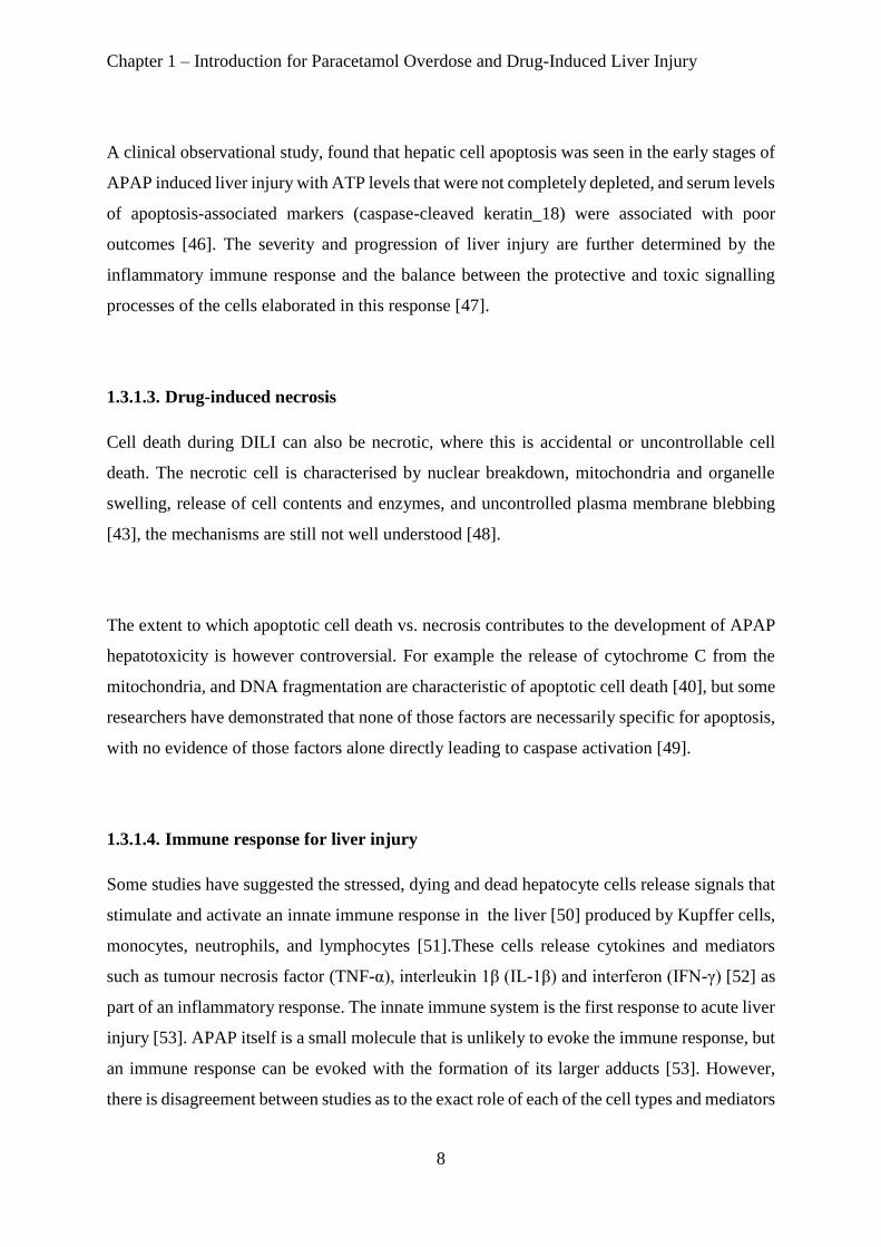
A clinical observational study, found that hepatic cell apoptosis was seen in the early stages of
APAP induced liver injury with ATP levels that were not completely depleted, and serum levels
of apoptosis-associated markers (caspase-cleaved keratin_18) were associated with poor
outcomes [46]. The severity and progression of liver injury are further determined by the
inflammatory immune response and the balance between the protective and toxic signalling
processes of the cells elaborated in this response [47].
1.3.1.3. Drug-induced necrosis
Cell death during DILI can also be necrotic, where this is accidental or uncontrollable cell
death. The necrotic cell is characterised by nuclear breakdown, mitochondria and organelle
swelling, release of cell contents and enzymes, and uncontrolled plasma membrane blebbing
[43], the mechanisms are still not well understood [48].
The extent to which apoptotic cell death vs. necrosis contributes to the development of APAP
hepatotoxicity is however controversial. For example the release of cytochrome C from the
mitochondria, and DNA fragmentation are characteristic of apoptotic cell death [40], but some
researchers have demonstrated that none of those factors are necessarily specific for apoptosis,
with no evidence of those factors alone directly leading to caspase activation [49].
1.3.1.4. Immune response for liver injury
Some studies have suggested the stressed, dying and dead hepatocyte cells release signals that
stimulate and activate an innate immune response in the liver [50] produced by Kupffer cells,
monocytes, neutrophils, and lymphocytes [51].These cells release cytokines and mediators
such as tumour necrosis factor (TNF-α), interleukin 1β (IL-1β) and interferon (IFN-γ) [52] as
part of an inflammatory response. The innate immune system is the first response to acute liver
injury [53]. APAP itself is a small molecule that is unlikely to evoke the immune response, but
an immune response can be evoked with the formation of its larger adducts [53]. However,
there is disagreement between studies as to the exact role of each of the cell types and mediators

Chapter 1 – Introduction for Paracetamol Overdose and Drug-Induced Liver Injury
9
in DILI. Generally, the mechanistic details of APAP induced liver injury have yet to be entirely
determined [36].
1.4. Clinical Assessment of APAP Overdose
Clinically, acute APAP overdose is associated with three main stages. The first stage takes
approximately 24 hours and is implicated by non-specific gastrointestinal (GI) symptoms, for
example, nausea, vomiting and abdominal pain, with insignificant elevation in serum liver
enzyme concentrations. The second stage takes about 24-72 hours, includes a few clinical
symptoms such as vomiting and abdominal pain, and elevation of serum liver enzymes
concentrations. The last stage develops in 72-96 hours post-ingestion, and the outcomes vary
from full recovery to death, which is based on the severity of liver damage [54].
Peak serum concentrations after therapeutic doses of APAP do not usually exceed 130μmol/L
(20 mg/L) [56], the elevation above this is an indication of overdose. N-Acetylcysteine (NAC)
is standard treatment for the liver toxicity effects of APAP overdose. NAC acts to replenish
glutathione levels in the liver which will be depleted by NAPQI production, preventing
accumulation of NAPQI and its toxic effects. The decision for treatment with N-Acetylcysteine
(NAC) based on blood APAP concentration typically uses the Rumack-Matthew nomogram
[55] (Left-Figure 1-3). This nomogram is used to guide the treatment of acute paracetamol
overdose provided time since overdose is known and uses information on high risk factors such
as alcoholism, malnutrition, liver disease etc.
In 2012, the UK revised the management of APAP overdose following the death of poisoned
patients who were considered not to be at significant risk [56] .The revised guidelines indicate
that all APAP overdose patients, regardless of risk factor-should be treated with NAC (Right-
Figure 1-3) [57]. This nomogram assessment technique is only applied four hours after APAP
overdose to ensure the full extent of the poisoning is understood after absorption. However,
only approximately 10% of patients present to the emergency department soon after APAP
overdose with the majority attending later than 12 hours [58]. Whilst the reported time of

Chapter 1 – Introduction for Paracetamol Overdose and Drug-Induced Liver Injury
10
overdose has a known associated error, the treatment is still based on this time. Importantly,
neither the dose of APAP or liver function tests (LFTs) are considered when making the NAC
treatment decision, when if they were a more precise, individualised treatment would be
possible based on the severity of overdose and effects on liver function.
Figure 1-3: Rumack-Matthew nomogram.
LEFT: Rumack-Matthew nomogram is based on high risk patients. The cut-off of NAC giving for high risk
patient is 100mg/l of APAP concentration at 4h post APAP ingestion and the cut off of NAC giving for non-
high risk patient is 200mg/l of APAP concentration at 4h post APAP ingestion.
RIGHT: Revise Rumack-Matthew nomogram. The cut-off of NAC giving for NAC is 100mg/l of APAP
concentration at 4h post APAP for all patients.
1.4.1. Current Biomarkers to Assess DILI
The current assessment of drug-induced liver injury or dysfunction in clinical practice uses
standard blood sample LFTs to quantify biomarkers to assess the degree of liver damage. These
tests include the serum concentration of total bilirubin (TBL), coagulation profile and the
activity assessment of the enzymes alkaline phosphatase (ALP), aspartate aminotransferase
(AST), and alanine aminotransferase (ALT) [59] with these enzyme activities expressed as
ratios to the upper limits of normal (ULN). A standard method of allocating cases is given
through the assessment of the normalised ratio of ALT to ALP activity, quoted as an R value.
R<2 is considered for cholestatic liver injury, while >5 is considered as hepatocellular injury
[60].

Chapter 1 – Introduction for Paracetamol Overdose and Drug-Induced Liver Injury
11
More specifically for APAP-induced liver toxicity the elevation of AST and ALT serum
concentrations to >1000 U/L is typically seen, as also are abnormal results of other LFTs [14],
with ALT being the more specific indicator for hepatocyte damage and thus the current gold
standard diagnostic and monitoring biomarker for APAP induced liver injury. Dear and
colleagues have added liver synthetic dysfunction, reflected in thrombin levels and blood
coagulation time, and summarised as the international normalised ratio (INR) for assessment
of liver damage. An INR >1.5 on top of ALT >100 is considered as reflecting liver toxicity as
well [61].
Even though the LFT blood tests can provide some evidence of the extent of the liver damage,
and their utility has been qualified by decades of clinical experience, there are still limitations
for using liver enzymes as biomarkers because changes in those enzymes’ activities are not
specific for DILI and may generate false positive results. LFT enzymes such as ALT can
change with different disease conditions of the liver such as viral hepatitis, fatty liver disease
and liver cancer [62]. They may also alter with a non-hepatic disease e.g. ALP may elevate
with hypothyroidism or bone disease [63] while ALT and AST increase with myocardial
disease [64] or muscle damage due to heavy exercise [65]. A combined approach of ALT and
INR represents the current standard for diagnosis of DILI.
1.4.2. Novel Biomarkers to Assess DILI
Despite the limitations, LFT blood tests can provide some evidence of the extent of liver
damage, and any novel biomarker must therefore surpass or provide added value to be a better
indicator of prognosis at presentation and during treatment. Consequently, there have been
recent pre-clinical and clinical studies that identify and validate biomarkers that show improved
sensitivity and hepatic specificity to assist of DILI [66]. These biomarkers may guide clinicians
to identify a patient who has low or high-risk of acute liver injury (ALI) who requires a lower
or higher treatment dose (of e.g NAC) or even no treatment at all.
Chapter 1 – Introduction for Paracetamol Overdose and Drug-Induced Liver Injury
12
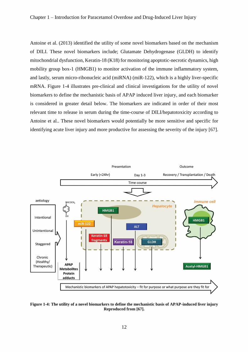
Antoine et al. (2013) identified the utility of some novel biomarkers based on the mechanism
of DILI. These novel biomarkers include; Glutamate Dehydrogenase (GLDH) to identify
mitochondrial dysfunction, Keratin-18 (K18) for monitoring apoptotic-necrotic dynamics, high
mobility group box-1 (HMGB1) to monitor activation of the immune inflammatory system,
and lastly, serum micro-ribonucleic acid (miRNA) (miR-122), which is a highly liver-specific
mRNA. Figure 1-4 illustrates pre-clinical and clinical investigations for the utility of novel
biomarkers to define the mechanistic basis of APAP induced liver injury, and each biomarker
is considered in greater detail below. The biomarkers are indicated in order of their most
relevant time to release in serum during the time-course of DILI/hepatotoxicity according to
Antoine et al.. These novel biomarkers would potentially be more sensitive and specific for
identifying acute liver injury and more productive for assessing the severity of the injury [67].
Figure 1-4: The utility of a novel biomarkers to define the mechanistic basis of APAP-induced liver injury
Reproduced from [67].

Chapter 1 – Introduction for Paracetamol Overdose and Drug-Induced Liver Injury
13
1.4.2.1. miR-122
miRNA are small molecules typically around 22 nucleotides long; they do not code for protein
and are usually involved in post-transcription gene product regulation [68]. The release of
miRNA into extracellular space and circulation can be an expression of a physiological process
(e.g. cell to cell communication) or indicative of liver injury [69].
miRNAs are widely expressed and appear to be highly organ specific. miR-122 is the most
abundant hepatic miRNA representing 75% of expression, and this marker is highly liver
specific [70]. The potential circulation of miR-122 was first reported in a mouse model after
APAP overdose [71]. In a clinical study, patients that developedALI (who had APAP overdose)
had around 100-fold higher serum levels of miR-122 than patients without ALI [72].
1.4.2.2. HMGB1
HMGB1 is a chromatin-binding protein released by cells undergoing necrosis [73]. It is
stimulated by the innate immune response and passively released as a cytokine [74]. In APAP
overdose mouse models it has been demonstrated that the circulation of HMGB1 is correlated
with onset of necrosis, confirming HMGB1 as a potential indicator in the cell death process
[75].
There is further evidence in mouse models that HMGB1 is a mechanism based biomarker and
also acts as a mediator of APAP hepatotoxicity, as administering anti-HMGB1 antibodies
reduced liver injury in a mouse model [42] and this might have potential for further
development as a therapeutic candidate for DILI.
In clinical evaluation, total HMGB1 is correlated strongly with ALT activity and prothrombin
time in patients with APAP-induced liver injury and the prognostic utility of elevation
acetylated HMGB1 associated with poor prognosis and outcome [76] .

Chapter 1 – Introduction for Paracetamol Overdose and Drug-Induced Liver Injury
14
1.4.2.3. GLDH
GLDH is an enzyme present in matrix-rich mitochondria of the liver and is a key enzyme in
amino acid oxidation [77]. In addition to the liver, GLDH is expressed in the brain and excreted
directly into cerebro-spinal fluid (CSF) [78], and expressed in kidney where it is excreted into
tubular lumen rather than into blood circulation [79]. Its presence in serum is considered a
relatively liver-specific marker and an indicator of leakage of mitochondria contents into
circulation associated with liver damage [80].
A rat model study indicated GLDH increased up to 10-fold after liver injury, and clinically, (in
cases with DILI) serum GLDH was shown to be increased, highlighting its potential as a
translational biomarker [81]. However, there still remains some indecision as to whether
measurement of GLDH could be valuable in distinguishing benign elevations in ALT from
those that portent severe DILI potential [82].
1.4.2.4. Keratin-18
Keratins are intermediate filament proteins that are expressed by epithelial cells and are
responsible for cell structure, differentiation and apoptosis [83]. K-18 is a form of keratin,
which is exclusively expressed in liver (representing 5% of total hepatic protein) and other
digestive epithelial cells [84]. There are two forms of K-18: fragmented caspase-cleaved (C
K18, commonly referred to an AK-18 for “Apoptosis-related K-18”) which represents the
apoptotic cell death mechanism, and full length (FL K18, commonly referred to a NK-18 for
“Necrosis-related K-18”), representing necrosis. These had been identified previously as novel
biomarkers, potentially more sensitive in DILI [85], and have been used in clinical situations
for therapeutic drug monitoring (TDM) of chemotherapy [86], and also for quantification of
apoptosis during liver disorders such as hepatitis [87].

Chapter 1 – Introduction for Paracetamol Overdose and Drug-Induced Liver Injury
15
Previously, in a mouse model, increases in both AK-18 and NK-18 were reported after APAP
overdose [75]. A group of clinical researchers confirmed the circulating levels of both cleaved
and full length K-18 after APAP overdose could be correlated with the poor outcome (i.e. death
or liver transplant) [46]. Recent evidence also suggested that modelling the ratio between AK-
18 and NK-18 may provide an important tool to help risk prediction of liver injury safety sign
during clinical trial [88].
1.4.2.5. Reference interval values for novel biomarkers.
The reference intervals for the novel biomarkers have been identified from a cross-sectional
study that involved 200 healthy volunteers and each individual subject across an intensive 24h
sampling period [61]. The data are expressed as 2.5th, 50th and 97.5th quantile each with a 90
% CI (confidence interval).
Table 1-1: Reference intervals for biomarkers of DILI
Biomarkers 2.5th quantile
(90 % CI) 50th quantile
(90 % CI)
97.5th quantile (90 % CI)
miR-122 (let-7d normalised)
0.17 (0.00 – 0.22) 0.95 (0.71 – 1.21) 6.40 (4.32 – Inf)
HMGB1 (ng/ml) 0.22 (0.17 – 0.32) 1.24 (1.16 – 1.29) 2.34 (2.23 - 2.42)
FL K18 (U/l) 114 (102 - 126) 248 (225 - 268) 475 (456 - 488)
CC K18 (U/l) 57 (53 - 60) 132 (122 - 142) 272 (256 - 291)
GLDH (U/l) 0.46 (0.30 – 0.56) 1.40 (1.30 – 1.46) 27 (26 - 30) CI is a confidence interval
1.5. Objectives and Aims
1.5.1. Overall Objective
The primary objective of this thesis is to transfer or link the bench science regarding novel
biomarkers of DILI into clinical practice by use of an applied population pharmacokinetics and
pharmacodynamics approach. Such methods will be applied to biomarker and APAP exposure
datasets obtained from the BIOPAR clinical trial that ran from November 2010 to October

Chapter 1 – Introduction for Paracetamol Overdose and Drug-Induced Liver Injury
16
2014 in ten different UK centres, and will be used to develop and test a rational approach to
estimate the time course of effects and biomarkers that can predict liver injury.
1.5.2. Specific Aims
1. To build population pharmacokinetics (Pop-PK) models using exposure data following
APAP overdose in a UK population to estimate mean population PK parameters such
as clearance and volume of distribution and quantify and assess their variability. This
will allow examination of the differences in exposure and PK parameters between
therapeutic doses and overdoses of paracetamol, an area yet to be fully explored in
current publications.
2. To build population pharmacokinetic-pharmacodynamic (Pop-PKPD) models using
biomarker data following paracetamol overdose to estimate PKPD parameters that
characterise the effect of paracetamol overdose on current and novel biomarkers of liver
function.
3. To simulate profiles for all novel biomarkers under the dosing of the BIOPAR dataset
using the Pop-PKPD model parameter estimates and compare with the ALT profile (as
the gold standard for liver injury) to identify potential earlier prediction of liver injury
with different biomarkers.
4. To simulate profiles for all novel biomarkers under different dosing regimens and
clinical scenarios to illustrate potential changes in the profile of biomarker effect.
5. To use Receiver Operating Characteristic ROC analyses for prediction of liver injury
as defined categorically by peak ALT status using simulated biomarker levels at various
timepoints and PKPD model parameter values. This will allow assessment of the best
potential timepoint for diagnosis of APAP induced liver injury and indicate the
potential value in the PKPD modelling approach.

Chapter 2 - Pharmacometric methods
17
Chapter-2
Pharmacometric Methods
Chapter 2 - Pharmacometric methods
18
Chapter 2. Pharmacometric Methods
2.1. Background
Pharmacometrics is the quantitative study of interactions between a drug therapy and the
subject it is administered to, where “drug therapy” means to use artificial or sometimes natural
agents that may change a physiological or biochemical body process. This in turn will hopefully
be useful to prevent or cure disease, however, if a drug is used inappropriately, it can be harmful
to the body. The effects of a drug are underpinned by the drug exposure and response. The drug
exposure is determined by the drug administration, which includes dose, frequency and route
of administration and the pharmacokinetics (PK) of the drug. Administration must be selected
carefully, with consideration of drug PK, to optimise the drug effect and at the same time
minimise harmful drug effects. The response refers to the biological changes induced by the
drug, and this response could be either a beneficial or an adverse effect. The quantitative study
of drug response driven by drug exposure is referred to as a drug’s pharmacodynamics (PD).
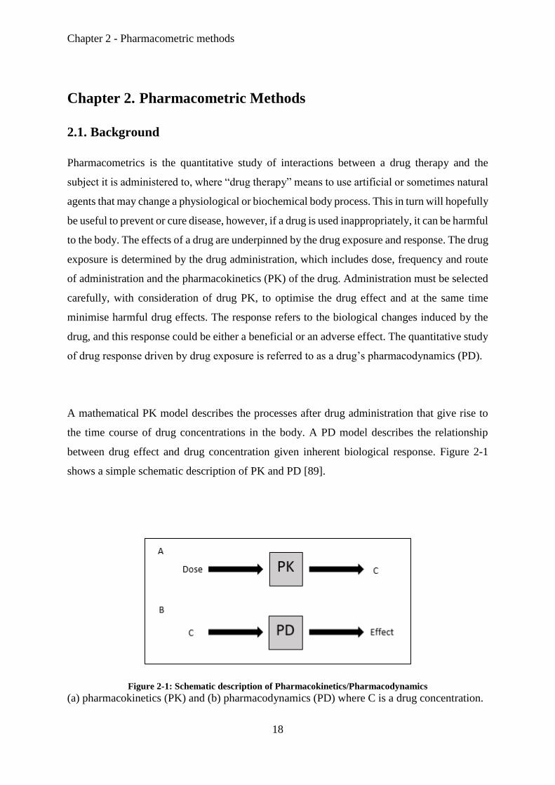
A mathematical PK model describes the processes after drug administration that give rise to
the time course of drug concentrations in the body. A PD model describes the relationship
between drug effect and drug concentration given inherent biological response. Figure 2-1
shows a simple schematic description of PK and PD [89].
Figure 2-1: Schematic description of Pharmacokinetics/Pharmacodynamics
(a) pharmacokinetics (PK) and (b) pharmacodynamics (PD) where C is a drug concentration.

Chapter 2 - Pharmacometric methods
19
PK and PD models share concentration as a common element. These two kinds of models can
be combined therefore in PKPD modelling to describe the time course of the dose-effect
relationship after any drug administration (Figure 2-2) [90].
Figure 2-2: Diagram description of the combination between PK and PD link together dose,
concentration and drug effect.
Understanding the dose-effect relationship of PK and PD following a therapeutic dose is the
primary goal in clinical pharmacology. The concepts of clinical pharmacology can be used to
design individual dose regimens to minimise adverse effects and optimise therapeutic response;
optimising the dose regimen includes the choice of the right dose and dosing interval.
2.1.1. Pharmacokinetics
PK is the study of how a drug enters, distributes and leaves the body, and can be considered
via four fundamental processes: absorption, distribution, metabolism and excretion (ADME)
(Figure 2-3). An understanding of how each of these processes may differ between individuals
needs to be accounted for in the design of an optimal dosing regimen for treatment [91].

Chapter 2 - Pharmacometric methods
20
Figure 2-3: The process of drug ADME.
An ingested drug undergoes absorption by passing through gastrointestinal membrane then through the liver
before reaching systemic circulation. Once it reaches the circulation, it distributes to the tissue, including the site
of action. Drug simultaneously undergoes metabolism and/or excretion, and this occurs primarily in the liver
and kidney. Reproduced from [91].
From a therapeutic viewpoint, the most critical factor for achieving the desired drug action is
the time course of drug concentration at the site of action. A PK model provides a mathematical
representation of this and relates the independent variables such as time and dose to the
dependent variable, plasma concentration, using pharmacokinetic parameters such as clearance
(CL) and volume of distribution (Vd). PK typically studies the time course of drug
concentration in the body simplified as a set of compartments [92] [93] where drug transfers
from one compartment to another. The central compartment represents blood/plasma and other
rapidly equilibrating tissues, receiving an input of drug either from an absorption process (often
modelled as a first-order process from a depot compartment) or via a direct dose (e.g.
intravenous bolus or infusion dosing (IV)). Peripheral compartments may be needed to describe
further distributional processes as necessary with each compartment having its own Vd to scale
the amount of drug contained to an observed concentration [94].

Chapter 2 - Pharmacometric methods
21
Compartments need not be directly physiological e.g. if the drug distributes rapidly out into
and back from the entire body the PK could be described with a single compartment. However,
if the drug returns more slowly after distribution into peripheral tissues one or more peripheral
compartments connected to the central compartment may be needed to describe the PK time-
course in a two, three (etc.) compartment models. These peripheral compartments can be
considered to represent physiological tissue compartments with similar distributional
characteristics that have been lumped together.
The equations below are examples of PK models for the central (i.e. plasma) compartment for
simple one compartment disposition under different modes of administration. Equation 2-1 for
an IV bolus, Equation 2-3 for a zero order IV infusion and Equation 2-3 for a first-order oral
absorption process, which is itself governed by the absorption rate constant (Ka). Elimination
half-life (t1/2) is another commonly discussed parameter and refers to the time required for the
plasma concentration to decrease by one-half and is derived from CL and Vd (Equation 2-4).
C(t) = Dose*e-(CL/Vd)*t Equation 2-1
C(t) = Rate/CL * (1-e-(CL/Vd)* t) Equation 2-2
C(t) = Dose*(Ka/Vd)*(Ka-(CL/Vd)) *[(e-(CL/Vd)*t)- e-Ka*t] Equation 2-3
t1/2 = 0.693/( CL/V) Equation 2-4
In the majority of cases, overall drug exposure (typically defined as the area under the curve
(AUC) of the measured concentration-time profile (AUCconc) increases or decreases
proportionally with the dose administered and this is called linear pharmacokinetics [95].
However, there are some drugs where exposures are disproportional to the drug dosage and
this phenomenon is called non-linear pharmacokinetics [96].
Chapter 2 - Pharmacometric methods
22
PK models can be used to help physicians to deal with the drug phenomena of linear or non-
linear pharmacokinetics. However, the time-course and magnitude of drug effect cannot
necessarily be predicted by the concentration time-course and the concept of clinical
pharmacodynamics is needed to describe the relationship between drug concentration and
effect.
2.1.2. Pharmacodynamics
2.1.2.1. Direct effect model
PD models describe drug effects as a mathematical relationship between drug concentration
and the drug’s potency and efficacy.
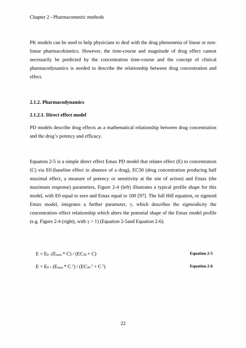
Equation 2-5 is a simple direct effect Emax PD model that relates effect (E) to concentration
(C) via E0 (baseline effect in absence of a drug), EC50 (drug concentration producing half
maximal effect, a measure of potency or sensitivity at the site of action) and Emax (the
maximum response) parameters, Figure 2-4 (left) illustrates a typical profile shape for this
model, with E0 equal to zero and Emax equal to 100 [97]. The full Hill equation, or sigmoid
Emax model, integrates a further parameter, γ, which describes the sigmoidicity the
concentration–effect relationship which alters the potential shape of the Emax model profile
(e.g. Figure 2-4 (right), with γ > 1) (Equation 2-5and Equation 2-6).
E = E0 +(Emax * C) / (EC50 + C) Equation 2-5
E = E0 + (Emax * C γ) / (EC50 γ + C γ) Equation 2-6
Chapter 2 - Pharmacometric methods
23
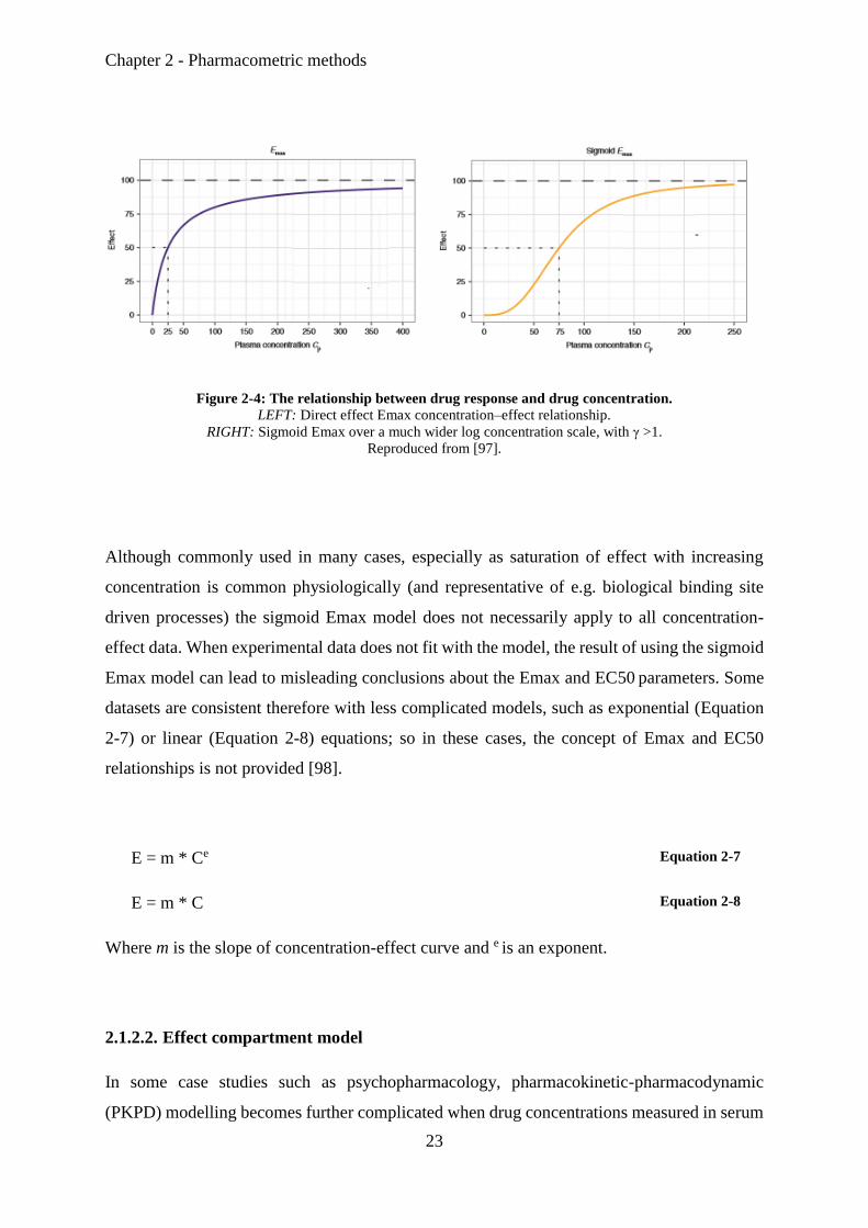
Figure 2-4: The relationship between drug response and drug concentration.
LEFT: Direct effect Emax concentration–effect relationship.
RIGHT: Sigmoid Emax over a much wider log concentration scale, with γ >1.
Reproduced from [97].
Although commonly used in many cases, especially as saturation of effect with increasing
concentration is common physiologically (and representative of e.g. biological binding site
driven processes) the sigmoid Emax model does not necessarily apply to all concentration-
effect data. When experimental data does not fit with the model, the result of using the sigmoid
Emax model can lead to misleading conclusions about the Emax and EC50 parameters. Some
datasets are consistent therefore with less complicated models, such as exponential (Equation
2-7) or linear (Equation 2-8) equations; so in these cases, the concept of Emax and EC50
relationships is not provided [98].
E = m * Ce Equation 2-7
E = m * C Equation 2-8
Where m is the slope of concentration-effect curve and e is an exponent.
2.1.2.2. Effect compartment model
In some case studies such as psychopharmacology, pharmacokinetic-pharmacodynamic
(PKPD) modelling becomes further complicated when drug concentrations measured in serum

Chapter 2 - Pharmacometric methods
24
or plasma do not reflect the concentration at the site of action or effect [98]. For example, the
relationship between concentration and time in the PK of lorazepam in plasma was
appropriately modelled with a two-compartment model, however studies on the effect of
lorazepam on electroencephalogram (EEG) suggested a delay in equilibration of lorazepam
between plasma and the site of PD action in the brain [99], therefore, the distribution of
lorazepam to its site of action might represent a rate-limiting process. The drug site of action
is often referred to as the biophase, as represented first by Furchgott [100].
The addition of a hypothetical effect compartment is one concept used to describe this delay
and this mathematical approach was demonstrated by Sheiner and colleagues [101]. The effect
compartment model is an additional compartment driven from the central compartment of a
PK disposition model by a first order rate constant parameter (Ke0) that governs the delay
process.
Outlined below are the differential equations to describe an effect compartment PD model
combined with a one compartment PK model with oral dosing, where Equation 2-9 describes
the gut dosing depot amount, Equation 2-10 the central compartment plasma concentration (Cp)
after oral dose, and Equation 2-11 the theoretical effect compartment concentration (Ce).
dDepot/dt = -Ka * Depot Equation 2-9
dCp/dt = Ka*Depot/Vd – Kel * Cp Equation 2-10
dCe /dt = Ke0*Cp –Ke0*Ce Equation 2-11
The initial condition for the Depot compartment amount is D x F, where D is drug (e.g. APAP)
dose amount and F the bioavailability, which is the fraction that reaches systemic circulation
intact. Cp is the concentration of drug in the central (plasma) compartment of the
Chapter 2 - Pharmacometric methods
25
pharmacokinetic model with Ka as the apparent first-order absorption rate constant for input
flow from the depot and Kel is the elimination rate constant given by clearance divided by
volume of distribution.
Ce is the theoretical concentration of the drug in the effect compartment with Ke0 as a rate
constant that links between the PK model and the effect compartment, which can be considered
to represent a delay/activation/deactivation process from the driving PK concentration. The
theoretical effect compartment is not part of the formal mass balance PK model of the drug and
does not contribute to the model of the drug PK disposition (hence why it may be called a
“theoretical concentration”). However it can often be thought of as representing the delay of
drug distribution into the biophase, or site of action, and could be more formally considered as
a “theoretical concentration that is the direct input to the PD model of drug effect”. It can also
be imagined to represent the delay of receptor activation or other drug effect processes (e.g.
protein expression).
Other PKPD models may be able to use the true PK mass balance model for a peripheral PK
distribution (or tissue) compartment as the direct input to a PD model of drug effect, however
this is not considered an effect compartment model, as here a “true” concentration is being used
as the driver of PD effect so this is instead a form of direct effect PKPD model. The relation
between the theoretical effect compartment of the drug concentration (Ce) and observed effect
can then described by whichever PD model may be appropriate e.g. a sigmoid Emax equation
(Equation 2-5).
Figure 2-5 shows a representation of the resultant pharmacokinetic-pharmacodynamic model
for the lorazepam study.

Chapter 2 - Pharmacometric methods
26
Figure 2-5: Schematic representation of the pharmacokinetic-pharmacodynamic model for lorazepam.
Lorazepam has a two compartment PK model, with reversible distribution to/from a peripheral compartment,
and first-order elimination (clearance) from the central compartment (rate constant: Ke). Plasma was assumed to
equilibrate with and then leave with a hypothetical effect site according to a first order rate constant (Ke0). Link
models (exponential and linear) for PD effect are then driven by effect site hypothetical concentration.
Reproduced from [102].
2.1.2.3. Indirect response model
Indirect response PD models were developed to characterize drugs that act by indirect
mechanisms such as inhibition or stimulation of the production or dissipation of factors
resulting in the measured effect [103] and a general form of this model was demonstrated by
Sheiner and Verotta [104]. Indirect response models are useful where a further delay, lag or
onset process needs to be described as part of the PD response, and also where a PD response
represents a perturbation from, and potential return to, a baseline physiological value.
The indirect effect model describes the rate of change of the response variable as a balance
between its apparent rate of “production” and its rate of “removal” (Equation 2-12)
dR/dt = Kin – Kout * R Equation 2-12

Chapter 2 - Pharmacometric methods
27
Dayneka and colleagues were the first to formally propose four basic variations of the indirect
response model [105] regarding where and how drug effect may be implemented. These are:
Inhibition of production, Inhibition of removal, Stimulation of production and stimulation of
removal.
The inhibition variants often use the following inhibitory factor as a function of drug
concentration, I(C) (Equation 2-13) which is a variant of the previously described Emax model
(Equation 2-5).
I(C) = 1 – (Emax * Cp) / (EC50 + Cp) Equation 2-13
The stimulation variants use a stimulatory factor as a function of drug concentration S(C)
(Equation 2-14).
S(C) = 1 + (Emax * Cp) / (EC50 + Cp) Equation 2-14
The four indirect response model variants (Equation 2-15, Equation 2-16, Equation 2-17
andEquation 2-18) are then defined by the following differential equations according to where
the inhibitory or stimulatory factors are incorporated:
dR/dt = Kin * I(C) – Kout * R Equation 2-15
dR/dt = Kin –Kout * I(C) * R Equation 2-16

Chapter 2 - Pharmacometric methods
28
dR/dt = Kin * S(C) – Kout * R Equation 2-17
dR/dt = Kin – Kout * S(C) * R Equation 2-18
2.2. Population Modelling Approaches
During the last four decades, the concept of combined PKPD modelling has been extended
further with its application in a population approach. Population Pharmacokinetics (Pop-PK)
is the study of the variability of drug concentrations amongst individuals when standard dose
regimens have been administered [106]. The primary goal of population pharmacokinetic
modelling is to quantitatively assess pharmacokinetic model parameters, their sources of
variability, and their effects on exposures by applying population analysis approaches to PK
data [107]. Population PKPD (Pop-PKPD) modelling seeks to do a similar form of analysis,
but to deliver an understanding of the corresponding pharmacological/therapeutic response
with a description of the variability of individual drug response from the mean response across
the population.
The understanding derived from a Pop-PK/Pop-PKPD analysis regarding the quantitative
relationship between drug input patterns, patient characteristics, drug disposition and response
is key to identify sources of variability, and these relationships can influence understanding of
drug safety and efficacy. Such understanding can also help improve the process of drug
development by implementing more informative designs and analyses and should be part of
general good therapeutic practice [115].
There are potential factors that can cause variability in exposure and response, altering dose-
concentration-effect relationships from individual to individual. Type of factors include:
patient features: e.g. body weight, surface area, race, sex, and age;
pathophysiological features: e.g. hepatic or renal impairment and specific diseases;

Chapter 2 - Pharmacometric methods
29
environmental factors: e.g. smoking, diet, and exposure to pollutants;
genomic factors impacting drug-drug interactions or via hepatic metabolism: e.g.
polymorphic cytochrome P450 isoforms of varying abundance from individual to
individual, such as CYP2D6, and CYP2C19 [114].
By incorporating information from data obtained from clinical monitoring of these patient-
specific factors and characteristics as covariates in a Pop-PKPD model, we can consider their
effects and can allow for these patient characteristics to have an associated effect on ADME or
efficacy parameters [108]. This understanding can play an important role in direct patient care
in providing quantitative or semi-quantitative guidelines for individualising and/or optimising
dosing therapies, which may be considered a key aspect of personalised or stratified medicine.
Pop-PK models can also be applied in therapeutic drug monitoring, designing dosing guidelines
for drug labelling, and in comparing the effect of competing dosing regimens on clinical trial
outcomes [116][117].
Currently, the Pop-PK/Pop-PKPD field has a significant number of methods and techniques
for analysis of preclinical and clinical data, as well as for clinical design optimisation, with the
development of specific mathematical methods and software packages. Historically however,
Pop-PK as an approach began with the pioneering work of Sheiner and his colleagues in 1972
[109] who developed the NONMEM software package in applying the population approach to
PK data. These methods were improved throughout the 1970s [106] and then in 1980s, as Pop-
PK became more widespread in use due its application to improve TDM and the drug
development process [110]. In February 1999, the US Food and Drug Administration (FDA)
published a ‘Guidance for Industry: Population Pharmacokinetics’ that provided mechanisms
for Pop-PK analysis and outlined its role in drug development. This guidance illustrates when
to perform and how to design and execute a Pop-PK study, how to analyse the data, what kind
of model validation procedures are available and how to write a documentation report.

Chapter 2 - Pharmacometric methods
30
A Pop-PK analysis is different compared to traditional pharmacokinetic analysis methodology,
which usually involves studying large numbers of homogenous patients to assess the PK of a
drug in relevant populations, using data analysis methods such as statistical moments, sums of
exponential modelling, as well as compartmental approaches and physiologically based PK
modelling. The fundamental approach of population pharmacokinetics is not to homogenise
and/or standardise the patients from which the data is collected, but to deliberately apply a
population analysis approach that describes and accounts for variability in the data thus
allowing the use of relevant information from all patients that is descriptive of those in whom
the drug may be used clinically [111]. Studying a population enables analysis of the variability
in PK and PD that occurs within and between patients, which should be identified, explained
and quantified for all potential sources. Pop-PK model development will typically involve an
initial phase where criteria and rationale for the choice of model are set, and the steps taken to
build the model are outlined, that will involve exploratory data analysis where statistical and
graphical procedures are used to uncover patterns and features in the population data [113].
Subsequent model validation is where the objective is to examine if the model reasonably
describes the data and produces a good fit [107].
Pop-PKPD analysis uses multistage hierarchical models, where the PK or PKPD mathematical
model parameter values of any individual patient will vary from the expected population values
because of inter-individual variability (IIV) [111] and possibly because of within-subject
variability (WSV) in parameters. WSV could arise, for example, from systematic errors in drug
dosing, or sampling or concentration measurement variation in samples from the same
individual but taken or analysed from separate clinical visits. WSV reflects a random change
in a patient’s PK parameter values at different times [112] where these random variations can
also arise because the mathematical model being applied to the data could be an
oversimplification of reality [113]. Population approaches can be used to parameterise IIV and
identify if potential sources of variability can make a proportion of IIV predictable via
covariates in some way, and identify the non-predictable proportion of IIV (which is thus
apparently random). For example, using weight as covariate could account for a predictable
component of IIV and thus predict a proportion of overall parameter variability. Predictable
variability is most commonly better understood for drug elimination processes and often uses

Chapter 2 - Pharmacometric methods
31
subject factors such as weight, renal function, and co- medications as covariates to help account
for IIV. Non-predictable variability is usually larger than the predictable variability explicable
in some way by covariates [119].
Population modelling approaches seek to define population distributions to describe IIV. Data
(e.g. drug concentrations, biomarkers) are collected from the specific population who have
taken a drug. The drug’s behaviour (PK, PD or both) is described by a (typically nonlinear)
mathematical model dependent on an unknown subject-specific parameter vector (θ), which
varies between subjects to take into account the variability of the drug response in the
population. This population variability in PK/PKPD response (based on clinical data) is
determined by the population parameter distribution function F(θ). The distribution F describes
the variability of parameter values across the population and provides estimates of their means
and confidence intervals (CI) [106]. The variation in these parameter values among the
population is then translated by the mathematical PK or PKPD model into variability in
observed response.
Population analysis methods can be classified into nonparametric and parametric methods
according to the assumptions made regarding the F(θ) distribution [107] and each classification
can be sub-divided into maximum likelihood or Bayesian approaches [108]. In the next
sections, different population analysis methods will be reviewed with focus given to the
methods applied in this thesis.
2.2.1. Nonparametric Methods
Nonparametric methods are not based on parameterised families of probability distributions;
and include descriptive statistics, statistical models, inference and statistical tests. These
methods make no (or very limited) assumptions about the shape of the F(θ) parameter
distributions across the population; sometimes even being referred to as distribution-free
methods. This approach can make predictions more robust in the sense that they do not depend
on whether or not the underlying distribution is normal or of any other specific type [109].

Chapter 2 - Pharmacometric methods
32
Therefore, they may be preferable when the assumptions required for parametric methods are
not valid and should be considered especially with sparse data [110]. Non-parametric methods
estimate the entire joint F(θ) distribution from the data directly, and are useful when the data
are strongly non-normal or resistant to transformation. Hence, they can be useful for dealing
with unexpected outlying observations that might be problematic with the parametric approach
[111] and may consequently detect possible subpopulations within data (e.g. fast and slow
metabolism) as a set of mixture models and are sensitive detectors of bimodality [112].
Additionally, non-parametric methods are useful in the analysis of ordered categorical data in
which assignation of scores to individual categories may be inappropriate, for example, in
analysing alcohol consumption data where directly used categories include never, a few times
per day, weeks etc [111]. Two of the more powerful nonparametric methods that can give
mathematical model parameter estimates from raw data are non-parametric maximum
likelihood (NPML) and nonparametric estimation-maximisation (NPEM). These can be
applied to patient care to optimise dose regimens for therapeutic effect [113].
The main problem with nonparametric methods are that parameter distributions across a
population often do not have a continuous and smooth shape particularly in relatively small
population datasets [114] which can lead to difficulty in characterising multiple sources of
variability [108]. Also, they may lack power compared with other forms of analysis, and this
may be a concern if the sample size is small or if the assumptions of a corresponding parametric
method such as normality of data do hold [110]. Also although using nonparametric methods
may be used to estimate parameter values to describe data, it is less straightforward to define
confidence intervals associated with these estimates when using this approach [111].
2.2.2. Parametric Methods
Parametric methods are based on the assumption that the F(θ) distribution being applied to
describe population data across individuals is a defined, parameterised probability distribution.
These distributions are defined principally by a measure of their central tendency such as mean,
median, mode combined with a measure of their spread, often standard deviation (SD), that
broadly describes the dispersion of this central tendency [115]. Parametric methods assume
Chapter 2 - Pharmacometric methods
33
that all random quantities are from known families of probability distributions and this known
functional form defines the relationship between observed responses across a population and
input variables [116].
A significant strength of a parametric approach is the ability to separate or partition IIV, WSV
and residual error. However, a major weakness is in only obtaining a point estimate for
parameter values with some associated standard error. This form of parameter estimate may
not be the best reflection of the potential uncertainty or variability in a parameter value, which
for example in a PK or PKPD modelling scenario might lead to an unrealistic prediction or
simulation of concentration or response. Furthermore, some argue this method lacks a desirable
property of mathematical consistency [117], and also the assumption of the distributional shape
inherent to parametric methods can be inaccurate for some PK parameters [108].
Various parametric approaches exist for use in Pop-PK and Pop-PKPD modelling, including:
the Naïve Average Data (NAD) approach, Naïve Pooled Data Approach (NPD) two stage
approaches (such as standard two stage (STS) and global two stage (GTS)) [118], Bayesian
hierarchical approaches, and the nonlinear mixed-effect approach (NLME), of which the latter
is most widely used. An NLME model can quantify and describe inter-individual
PKPDvariability without neglecting potential difficulties associated with data (e.g. missing or
sparse data), which is a more reliable approach that is appropriate for the data in this thesis
because of the limitation of the dataset (section 3.2.4) compared to NAD, NPD etc.
2.2.2.1. The Nonlinear Mixed-Effect Model Approach (NLME).
NLME was first introduced for application to PK data by Sheiner and co-workers [119]. The
main goal of this approach is to model the relationship between a set of independent input
variables to some dependent variables as in any regression analysis. In the case of a Pop-PK
model, the dependent variable is concentration, and independent variables would be dose, time
and possibly some specific individual covariates such as age and weight. A Pop-PD model
provides the relationship of dose and concentration to some pharmacodynamic effect [120,

Chapter 2 - Pharmacometric methods
34
121]. An NLME approach considers the data as a study sample with the analysis providing for
estimation of the distribution of model parameters across the study population, defining their
potential relationship to covariates and characterising IIV, WSV and residual error. Analysis
can even be performed in a worst case scenario of a single datapoint per patient and data need
not follow any specific consistent sampling schedule [122].
The parameters of an NLME model are divided into two groups: fixed and random effect
parameters [123, 124]. Fixed effects parameters describe the central tendency of parameter
values for the whole population, providing average estimates of pharmacokinetic parameters
or the effects of covariates on them. Random effects parameters are used to describe the
variability between and within individuals in the population, i.e. IIV in parameter values from
the population mean values, WSV and residual error/variability composed of measurement of
errors, model misspecification, and intra-individual variability [125]. Despite not formally
being a true Bayesian approach the parameterised NLME model-based approach can also still
allow the inclusion of prior information via specialised methodologies, thus enhancing
understanding and statistical power.
In PKPD models the model relationship translating model parameter values into the response
variable is usually a nonlinear one [126]. Most nonlinear mixed-effects modelling methods
estimate the parameter values with a maximum likelihood approach [127], where an objective
function is defined that measures the goodness of fit of a particular model and parameter values
to a dataset. The global space of potential values for the parameters is searched to optimise the
objective function value giving the parameter values that best fit the data (depending on how
the objective function is defined this typically involves searching to minimise its value).
However, it is difficult to calculate the likelihood function for most PK models because of the
nonlinear relationship between random effects parameters for interindividual variability and
possibly residual variability as well. Therefore, to deal with these problems, various forms of
likelihood function approximation methods have had to be developed and implemented in the

Chapter 2 - Pharmacometric methods
35
NONMEM software package as described previously in the literature [128, 129]. These include
the first-order method (FO), first-order conditional estimation (FOCE) and Laplacian method
(LM).
The FO approach uses a linearization of the model in the random effects by using a first-order
Taylor series expansion taking into account random effect variables. The advantage of the FO
approach is that this “approximate likelihood” is available in a closed form solution. Standard
errors for the parameters are obtained from the Fisher information matrix assuming the
approximation is exact, and this method is suitable for initial estimation [116]. Compared with
the STS approach the FO approach provides better parameter estimation when increased
residual error leads to increased bias when using the STS approach [130]. However, the FO
approach leads to deterioration in residual error estimation [131]. On the other hand, one
compartment model experimental datasets showed similar results in population mean and
variance estimates with FO, GTS and Bayesian hierarchical modelling approaches [132]. The
main significant drawback to the FO approximation however, is deriving biased parameter
estimations especially when the distribution of inter-individual variability is specified
incorrectly [133].
The First-Order Conditional Estimation (FOCE) and the Laplacian Methods [134] are two
alternative maximum likelihood estimation methods implemented to reduce bias estimation
when the inter-individual variability is an increasing concern. FOCE uses a first-order Taylor
series expansion around the conditional estimates of the differences between the population
and the individual parameters (inter-individual random effects), then population, fixed effects
parameters and random-effects parameters are estimated at each iteration step [135]. This
estimation involves an iterative generalised least-squares type algorithm [122]. The more
advanced, modified FOCE with Interaction (FOCEI) method additionally allows the
dependence of random deviations between the individual predictions and the observed
measurements to be accounted for in the model fitting.
Chapter 3 - Population Pharmacokinetics Analysis of following APAP Overdose in U.K
Population
36
Chapter-3.
Population Pharmacokinetic
Analysis of following APAP
Overdose in U.K Population

Chapter 3 - Population Pharmacokinetics Analysis of following APAP Overdose in U.K
Population
37
Chapter 3. Population Pharmacokinetic Analysis of APAP
following Overdose in U.K Population
3.1. Introduction
Despite the safety and efficacy of APAP at therapeutic dose, evidence presented in section 1.1
suggests that it is the most common cause of drug induced liver injury through overdose [2].
APAP is a widely used medication present in preparations that can be either prescription or
non-prescription medications and also used in thousands of over-the-counter (OTC) products.
For prescription medication, it can be combined with morphine to provide very effective
analgesia for intense pain while minimising the potential for unwanted side effects of using
opiates such as respiratory depression [136]. Non-prescription APAP, is indicated for pain,
fever and symptoms associated with colds, flu, and allergies. It is considered a safe medication
when dosed as directed with the recommended dose of APAP being 4 g (or 75 mg/kg) in 24
hours for an adult patient. Perhaps because of its ease of availability, APAP is one of the most
frequently used drugs in intentional overdoses that are associated with drug-induced liver
injury [137]. Overdose can occur after single acute ingestion of a significant amount of APAP
or repeated ingestion of an amount exceeding recommended dosage. Acute single overdose is
defined as ingestion of >4 g (or >75 mg/kg) in a period of <1 hour [138].
The primary objective in this chapter was to describe the pharmacokinetic profile of APAP in
a UK group of overdose patients, to support PKPD modelling of DILI biomarker data as part
of a sequential, two stage PKPD analysis. It was also of particular interest to find out how much
the PK parameters following overdose dose of APAP are changed compared to patients
receiving a therapeutic dose and a key secondary objective was also to identify changes in the
PK parameters of CL and Vd as a function of measured covariates.

Chapter 3 - Population Pharmacokinetics Analysis of following APAP Overdose in U.K
Population
38
3.2. Materials and Methods
3.2.1. Subjects
Subjects were selected from the BIOPAR NHS portfolio prospective study as previously
described [61]. The study was carried out as part of the Biomarkers of Paracetamol
Hepatotoxicity Clinical Trial, run from November 2010 to October 2014 in ten different UK
centres: Royal Blackburn Hospital, Furness General Hospital, Newcastle Hospitals NHS
Foundation Trust, Poole Hospital, Royal Bournemouth & Christchurch Hospitals, Royal
Devon & Exeter Hospital, Royal Liverpool & Broadgreen University Hospital NHS Trust,
South Devon Healthcare NHS Foundation Trust, St. Helens & Knowsley Teaching Hospitals
NHS Trust and University Hospitals of Morecambe Bay. The local ethics committee
prospectively approved the study and all patients engaged in the study were required to give
written informed consent. Patient information sheets and consent forms were submitted for
review and approved by the North West Centre of Research Ethics Committee.
The inclusion criteria for this trial were: patients to be 18 years old or over, the subject being
willing to take part, diagnosis of paracetamol overdose (as defined by > 4g taken in 24 hours)
and written informed consent obtained. Exclusion criteria were: patient unwilling to take apart,
and/or unable to consent and the subject being not suitable to participate in the study in the
opinion of the investigator.
Patients were recruited over a period of 3 years, all patients who enrolled with APAP overdose
were treated with N-acetylcysteine and each patient was followed up for a maximum of six
months following discharge from the hospital
3.2.2. Sample Collection, Measurement and Storage
Two 10 mL blood samples were required at time of presentation, or 4 hours after estimated
paracetamol overdose, before administration of N-acetylcysteine. A further blood sample was

Chapter 3 - Population Pharmacokinetics Analysis of following APAP Overdose in U.K
Population
39
drawn at 12-18 hours after the first, and then followed by samples at 9.30am each day of
hospitalisation of the patient. Samples were used to measure APAP plasma concentration and
liver injury biomarkers that included the current standards (ALT and INR).
The first sample was collected in a Lithium/heparin coated vacuette collection tube (for plasma)
then stored at 4˚C upto 72hr before the occurrence of significant haemolysis, and the second
sample onwards collected in plain vacuette collection tubes (for serum). Samples were stored
at -800C until analysis.
Patients with liver damage (as evidenced by raised transaminases and/or abnormal clotting)
were kept in hospital until liver tests showed consistent signs of improvement. These patients
had regular monitoring of liver function; in these patients, blood samples were collected every
48 hours (2 x 10mL of blood for proteomic analysis together with a urine sample) up to a
maximum of 2 weeks post-admission.
3.2.3. APAP Measurement
APAP was extracted as described previously [139] from plasma using a liquid-liquid method
with acidified methanol [26] adding 10 µg APAP-d4 (APAP-d4) and 10 µg APAP-SUL-d3 as
internal standards and vortex mixed into 10 µl plasma with 0.8 mL methanol.
The analysis was carried out by liquid chromatography-tandem mass spectrometry (LC-
MS/MS) all reagents were purchased from Fisher Scientific, UK. APAP concentration was
quantified using a high-performance liquid chromatographic assay, the separation was
achieved by using an Aria CTC auto-sampler, and Allegros pump on an ACE Excel 2 SuperC18
column. The wavelength of detection was fixed at 244 nm on a Waters 486 Absorbance
Detector (Waters Ltd, Elstree, UK) to quantify the analyses.

Chapter 3 - Population Pharmacokinetics Analysis of following APAP Overdose in U.K
Population
40
3.2.4. Dataset Limitations and Caveats
It should be noted at this point that there are various limitations with this dataset including a
lack of access to the original source databases to address some specific queries regarding e.g.
patient monitoring, ethnicity, and time of NAC dosing. The dataset was an uncontrolled cohort,
in the sense that it was observed directly in genuine overdose patients and therefore had no
control regarding (over)dose levels or controlled monitoring of time of ingestion. This led to a
dataset subject to a high degree of noise, and with a large degree of uncertainty regarding actual
dose times and dose levels, which would have to be accepted as declared (in the absence of any
other information) despite potentially being incorrect.
Because of these limitations, spare dataset and the lack of published references covering PKPD
modelling of the novel biomarkers being examined, a parametric NLME population modelling
approach implemented in NONMEM was chosen as the most appropriate for the various PK
and PKPD modelling work in this thesis, having the potential to adapt or account for
deficiencies in the dataset better than other approaches.
3.2.5. Population Pharmacokinetic Models
A Nonlinear mixed effects (NLME) approach implemented in NONMEM was used for all
population pharmacokinetic analyses. As outlined in Chapter 2 (2.2.2.1) and two estimation
methods were used for parameter estimation: first-order conditional estimation method (FOCE)
and first-order conditional estimation with interaction method (FOCEI).
3.2.6. NLME Structural and Statistical Model Development
The population model in the NLME approach is typically divided into three hierarchical sub-
models. These sub-models are: structural sub-model, statistical sub-model and covariate sub-
model. The figure below shows a schematic outline of this form of population pharmacokinetic
model (Figure 3-1).

Chapter 3 - Population Pharmacokinetics Analysis of following APAP Overdose in U.K
Population
41
Figure 3-1 - Schematic outline of a Population Pharmacokinetics model.
3.2.6.1. Structural sub-model
The first step in a population pharmacokinetics analysis is to build the structural sub-model.
This model is characterised by fixed effects parameters that would describe the central
tendency of the data, measured in the absence of covariates. These fixed effects parameters are
often considered “population mean parameters” that describe the PK profile over time in a
typical individual (Equation 3-1).
Fpop,j = ƒ (θ, Xj) Equation 3-1
where ƒ is a mathematical PK model function, describing the relationship between a given
vector of independent variables (Xj) such as time and dose, and the jth response of a typical
Population Model
Structural sub-model
Covariate sub-Model
Statistical sub-model
Variability
Interindividual Interoccasion Residual
Chapter 3 - Population Pharmacokinetics Analysis of following APAP Overdose in U.K
Population
42
individual according to a vector of fixed effect model parameters θ (coded as THETA in
NONMEM) containing values such as e.g. typical clearance and typical volume distribution.
During exploratory data analysis, one and two compartment models with first-order absorption
were fitted to APAP data in NONMEM to determine the best structural model, and a two-
compartment structural model was not well supported by the data (poor precision of parameter
estimates), this is consistent with the sparseness and degree of noise in the data. PK models
were parameterised in terms of clearance and volume of distribution using the TRANS2 option
of PREDPP subroutines supplied in NONMEM. ADVAN2 ‘one-compartment model with
first-order absorption’ was used [140].
3.2.6.2. Statistical sub-model
This sub-model seeks to describe and quantify the variability in response between and within
patients, and any residual variability, by the estimation of random effects parameters. The
random effects parameters are represented in a variance-covariance matrix. Three types of
variability are typically characterised in this sub-model: variability among individuals which
is quantified by the interindividual variability (IIV), variability within individuals between
occasions which is quantified by the within subject variability (WSV) and residual variability
(RV), also commonly called residual error, which is due to non-measurable and uncontrollable
factors such as uncertainty in measurements or inaccuracy in dosing amount [141].
IIV describes how individual’s parameter values in the PK model are different from each other.
In the analyses in this thesis, IIV was modelled as an exponential random effect to make sure
all individual parameters are strictly positive ( Equation 3-2) which is coded in NONMEM as
Equation 3-3. This is broadly equivalent to the parameters having a log-normal distribution
across the population of individuals.

Chapter 3 - Population Pharmacokinetics Analysis of following APAP Overdose in U.K
Population
43
θi = θpop * exp(ηi) Equation 3-2
θi = TVθ* EXP (ETA (1)) Equation 3-3
where θi represents the PK model parameter value θ for the individual i, and θpop and TVθ are
the fixed effect, “typical value” of that parameter for the population. ηi (coded as ETA) denotes
the interindividual-difference between θi and θpop and is drawn from a normal distribution with
mean of zero and variance ω2, which is estimated by NONMEM as a random effects parameter
(coded as OMEGA).
Extending Equation 3-1, we define the individual response for a given set of independent
variable values (time, dose etc.) in Equation 3-4:
Fij = ƒ (θi, Xij) Equation 3-4
Residual variability/error is the variability that remains unexplained by the model thus far and
may rise from random errors in dosing and sampling of patients, from data being collected over
an extended period, or analytic assay variability.
Four different types of residual error models were used in the analyses. These models were
additive ( Equation 3-5), proportional (Equation 3-6), exponential ( Equation 3-7) and
combined additive and proportional ( Equation 3-8).
Yij = Fij + εij
Equation 3-5

Chapter 3 - Population Pharmacokinetics Analysis of following APAP Overdose in U.K
Population
44
Yij = Fij * (1 + εij) Equation 3-6
Yij = Fij * exp(εij) Equation 3-7
Yij = Fij * (1 + ε1ij) + ε2ij Equation 3-8
where Yij and Fij represent the jth observed and model-predicted concentrations for the ith
individual, respectively. εij is the residual random error for individual i and observation j and
is drawn from an independent normal distribution with a mean of zero and a variance of σ2,
which estimated by NONMEM as a random effects parameter (coded as SIGMA).
The equations above are coded in NONMEM as follows (Equation 3-9, Equation 3-10,
Equation 3-11 and Equation 3-12);
Y = F * EPS(1) Equation 3-9
Y = F *(1+EPS(1)) Equation 3-10
Y = F *EXP(EPS(1)) Equation 3-11
Y = F * (1+EPS(1)) + EPS(2) Equation 3-12

Chapter 3 - Population Pharmacokinetics Analysis of following APAP Overdose in U.K
Population
45
3.2.6.3. Covariate model
Once the base model (structural model plus statistical model) is identified, then the influence
of the subject-specific covariates on PK parameters can be assessed. Two kinds of covariates
were assessed in the data available: continuous and categorical [142]. The continuous
covariates examined included age and total body weight, while categorical covariates (some
simply binary) included sex, alcohol consumption, INR and LFT.
Covariate model selection is based on physiological rationale, clinical relevance and statistical
significance and is assessed by including the value of a covariate in the calculation of the typical
value of a structural model parameter in the overall model (i.e. at the level of the fixed effects).
Initial characterisation of a covariate relationship can be done visually with a graphical analysis
plotting individual model parameter estimates (θi from above) versus covariate values in those
individuals.
Physiological effects of clinical significance can be quantified by a covariate model for
example a percentage change in the typical value of a parameter in question for patients of one
categorical covariate value vs. another can be estimated (e.g. CL in male vs. female patients).
Incorporation of the covariate in the model should give a reduction in estimates of IIV and
residual error as previously non-predictable variability is now being “explained” by the
covariate information; potentially there should also be an improvement in the precision of
parameter estimates.
The statistical significance of the inclusion of a covariate in a model is based on the change in
objective function value (OFV). The OFV is a global measure of the goodness of fit of the
model to the data that calculates the differences between the observed and predicted values of
the dependent variable in question (for example with PK data, the observed drug concentration
and the concentration predicted by the model).

Chapter 3 - Population Pharmacokinetics Analysis of following APAP Overdose in U.K
Population
46
There are various different types of objective function and examples include: Ordinary Least
Squares (OLS); Weighted Least Squares (WLS); Penalized weighted least squares (PWLS),
Iteratively reweighted least squares (IRLS) and Extended Least Squares (ELS) [143].
NONMEM computes an ELS objective function, which it iteratively minimises by searching
the parameter space of the model parameter values to derive a set of parameter values that best
describe the data. This OFV is a form of maximum likelihood model fitting and the NONMEM
objective function is equivalent to -2 x log-likelihood.
The OFV is described by a chi-squared distribution. Therefore, a statistically significant
(α=0.05) difference in OFV indicating improved fit to the data is given by a drop of 3.84 for
one extra degree of freedom provided by one additional model parameter added compared to
the nested base model, (based on χ2α=0.05,υ=1). This is equivalent to a likelihood ratio test to
choose between two (mathematically nested) models as to which best fits the data based on the
minimum value of the objective function.
Covariates are added to a model stepwise, one at a time, observing the change in OFV, retaining
the covariate associated with the greatest fall in OFV until no further falls of 3.84 or more are
given. Backwards elimination may then be carried out where covariates are removed from the
“draft” final model one at a time looking for a more stringent degree of statistical significance
(e.g. χ2α=0.01,υ=1, critical value = 6.64) in order for them to be retained.
The clinical relevance and utility of a covariate in clinical practice may also be more important
than a statistically significant change in OFV [144]. By this criterion, for a categorical
covariate, a minimum 20% change in the affected model parameter in individuals of one
covariate category vs. another must exist for the covariate to be considered clinically
significant. Reduction in the magnitude of IIV in the parameter of interest (despite a potentially
small change in OFV) is also a consideration as we may choose to reduce unexplained
variability in the model by using the information in the covariate.

Chapter 3 - Population Pharmacokinetics Analysis of following APAP Overdose in U.K
Population
47
3.2.6.3.1. Continuous covariates
The effect of a continuous covariate such as age and weight is often expressed relative to its
median. The most common functional forms for covariate relationships are linear (Equation
3-13), power (Equation 3-14) and exponential (Equation 3-15) as following equations;
TVθ= θ + θcov * (COV-COVmedian) Equation 3-13
TVθ= θ * (COV/COVmedian) θcov Equation 3-14
TVθ= θ *EXP (θcov *(COV-COVmedian)) Equation 3-15
Where TVθ represents the population value of parameter θ for a specific covariate value (COV)
(e.g. the typical value of clearance for individuals of a specific weight), and θ is the population
value of the parameter for those individuals having a covariate value equal to the median value
(COVmedian) as for these individuals COV - COVmedian = 0 or COV/COVmedian = 1. θcov
represents the fractional change in the population parameter value as a result of the covariate
effect.
The equations above are coded in NONMEM as follows for linear (Equation 3-16), power
(Equation 3-17) and exponential (Equation 3-18) covariate relationships;
TVθ=THETA(1)*THETA(2)*(COV-COVmedian)
θ= TVθ *EXP(ETA(1))
Equation 3-16

Chapter 3 - Population Pharmacokinetics Analysis of following APAP Overdose in U.K
Population
48
TVθ=THETA(1)* (COV/COVmedian)** THETA(2)
θ=TVθ*EXP(ETA(1))
Equation 3-17
TVθ=THETA(1)*EXP(THETA(2)*(COV-COVmedian))
θ=TVθ*EXP(ETA(1))
Equation 3-18
TVθ is a typical value parameter with the median value of covariate (COVmedian). θ is a
parameter estimate, ETA(1) is a difference between individual and population of the parameter
estimate. THETA(2) is a factor describing the influence of covariate (COV).
3.2.6.3.2. Binary and categorical covariates
A binary covariate model was used for gender, INR and alcoholism categories (Equation 3-19)
and was coded in NONMEM as Equation 3-20 where the covariate category for a given
individual is described in the data file with a dummy variable value of 1 or 0.
TVθ= θj * θcov COV Equation 3-19
TVθ=THETA(1)*THETA(2)**COV Equation 3-20
If the categorical covariate model has n discrete values where n is greater than or equal to 3
(e.g, for ALT status in this dataset) (n-1) dummy variable values must be used in the dataset.
For example, ALT used two dummy variables, the first dummy is 1 for ALT >100 and < 1000
and otherwise 0, the second dummy being 1 if ALT > 1000 and otherwise set as 0 ( Equation
3-21) and coded as ( Equation 3-22). Individuals will either be COV1 = 0 and COV2 = 0 (for

Chapter 3 - Population Pharmacokinetics Analysis of following APAP Overdose in U.K
Population
49
those <100), COV1 = 1 and COV2 = 0 (for those >100 and < 1000) or COV1 = 0 and COV2
= 1 for those >1000.
TVθ= θj * θcov1 COV1
* θcov2 COV2 Equation 3-21
TVθ=THETA(1)*THETA(2)**COV1* THETA(3)**COV2 Equation 3-22
3.2.7. Dealing with Outliers
Outlier data are any observations that are unexpectedly different from other values. Outliers
and error are not synonymous however, and a value lying distinctly separate to a body of other
data points (often when visualised graphically) could arise from error, chance, or may reflect
general variation and represent a ‘true’ difference. Careful examination of a dataset can suggest
the likelihood of an outlier being an inaccurate value and assists whether or not the outlier
could instead be plausibly due to genuine biological variation.
The Z score (also known as a standard score) was used to exclude outlier data. The Z score is
given by Z = (mean - value) / SD, and quantifies how many standard deviations a value is from
the mean. With the data in this thesis, datapoints with Z-scores outside the range of +/- 2
standard deviations from the mean of all the observed data values were judged outliers and
were thus candidates for exclusion from analysis [145].
3.2.8. Model Validation
Model evaluation methods aim to assess the developed model for its fitness or quality in
describing the data. Model evaluation centres on graphical inspection plots (goodness of fit
plots or diagnostic plots) and assessment of the precision of model parameter estimates.
Diagnostic plots were created in R version (3.4.1). With plots providing visual inspection of
Chapter 3 - Population Pharmacokinetics Analysis of following APAP Overdose in U.K
Population
50
the following: how well the model population and individual predicted concentrations (PRED
and IPRE) match the observed data, conditional weighted residuals (CWRES) versus
population predictions (PRED) and versus time, clear identification of statistical outliers in the
raw data, and identification of covariate relationships.
Once a final model was selected, robustness and precision of parameter estimates was
evaluated using the nonparametric bootstrap approach carried out using the Perl Speaks
NONMEM (PsN) toolbox [128]. This form of bootstrap is a resampling method which was
first presented by Efron in the late 1970s for assessment of bias and precision [146]. The
method involves repeated random sampling with replacement from the input population data
file to create bootstrap datasets that are then fitted with the final mathematical model. The 95%
confidence interval (CI) for parameter estimates was calculated from percentiles (2.5th, 50th,
and 97.5th) of the empirical distribution of the estimated parameters from 1000 bootstrap
datasets run.
A visual predictive check (VPC) is a simulation-based diagnostic for all model components in
a population approach, mixed effects model with its origin in the posterior predictive check
(PPC) [147]. A VPC graphically compares the observations of a dataset with the prediction
interval generated by repeated simulations (typically n = 1000) of the dataset and its variability
based on the final fixed and random effects parameter estimates of the model fitting. Observed
data was plotted overlaid with 5th, 50th and 95th percentiles of the simulation data to allow visual
assessment of how the modelled fit describes the data and its variability.

Chapter 3 - Population Pharmacokinetics Analysis of following APAP Overdose in U.K
Population
51
3.3. Results
3.3.1. Data
202 patients were recruited in the BIOPAR clinical trial. Data from 94 of these patients with
non-staggered acute APAP overdose (i.e. a single ingestion overdose event) were then taken
forward for this analysis. The demographic data for all subjects are summarised in Table 3-1.
For the model-building process missing individual data were replaced by the median value of
the study population, which is a standard method when <10% of data is missing [148]. For
weight, there were 7 patients (7.4% of the study population) where this was required. The
median dose of APAP ingested was 32g (range 8-140g). 225 APAP plasma samples were
measured for concentrations and the median APAP plasma concentration at first presentation
was 33mg/L (range 2-500 mg/L). Histograms of age and weight across the individuals in the
dataset are shown in Figure 3-1.
Table 3-1: Summary statistics of BIOPAR patients’ characteristics.
Weight (kg) Mean (SD) 71.5 (19.6)
Median 66.68
Min, max 35, 171.4
Age (years)
Mean (SD) 12.4 (14.5)
Median 29
Min, max 18, 81
Gender Female n (%) 48 (51%)
Male n (%) 46 (49%)
Chronic Alcoholism
Yes n (%)
No n (%)
49 (52%)
45 (48%)
ALT
<100 (n) 87
>100 (n) 7
INR
<1.5 (n) 90
>1.5 (n) 4 (SD) Standard Deviation
(n) Number of patients
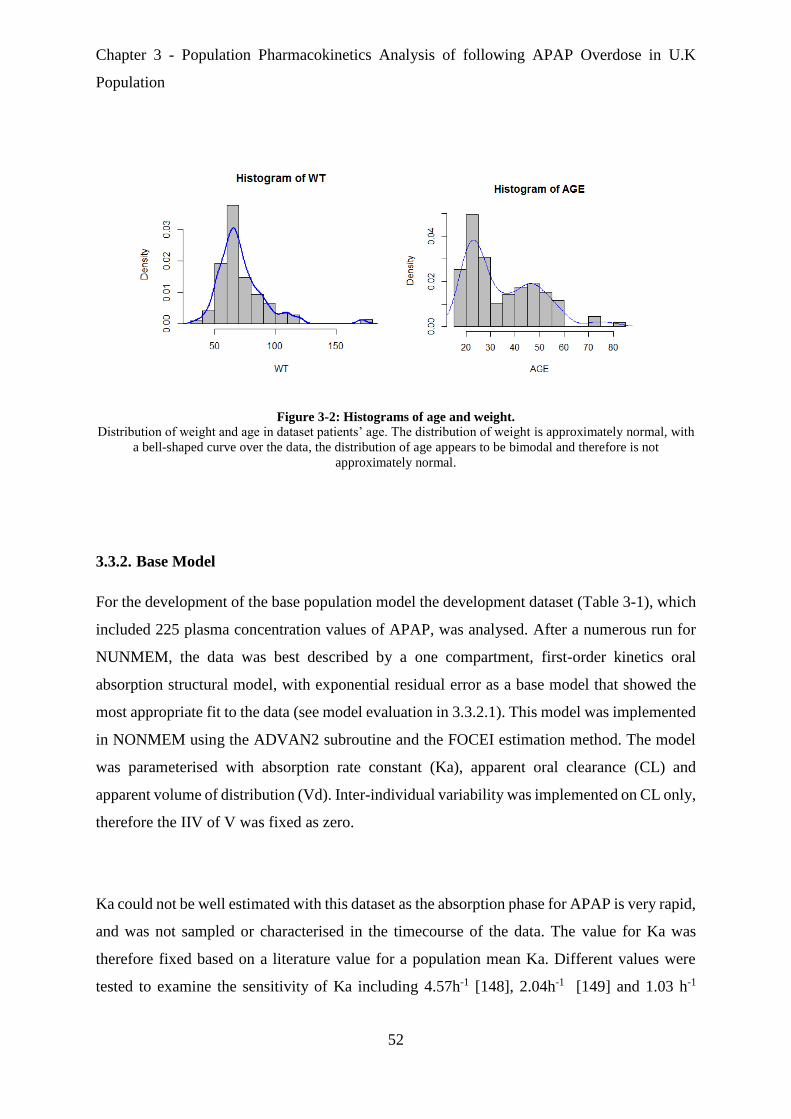
Chapter 3 - Population Pharmacokinetics Analysis of following APAP Overdose in U.K
Population
52
Figure 3-2: Histograms of age and weight.
Distribution of weight and age in dataset patients’ age. The distribution of weight is approximately normal, with
a bell-shaped curve over the data, the distribution of age appears to be bimodal and therefore is not
approximately normal.
3.3.2. Base Model
For the development of the base population model the development dataset (Table 3-1), which
included 225 plasma concentration values of APAP, was analysed. After a numerous run for
NUNMEM, the data was best described by a one compartment, first-order kinetics oral
absorption structural model, with exponential residual error as a base model that showed the
most appropriate fit to the data (see model evaluation in 3.3.2.1). This model was implemented
in NONMEM using the ADVAN2 subroutine and the FOCEI estimation method. The model
was parameterised with absorption rate constant (Ka), apparent oral clearance (CL) and
apparent volume of distribution (Vd). Inter-individual variability was implemented on CL only,
therefore the IIV of V was fixed as zero.
Ka could not be well estimated with this dataset as the absorption phase for APAP is very rapid,
and was not sampled or characterised in the timecourse of the data. The value for Ka was
therefore fixed based on a literature value for a population mean Ka. Different values were
tested to examine the sensitivity of Ka including 4.57h-1 [148], 2.04h-1 [149] and 1.03 h-1

Chapter 3 - Population Pharmacokinetics Analysis of following APAP Overdose in U.K
Population
53
[150]. The best fit for basic structure model was given by fixing the absorption rate to a value
of 4.57h-1.
The mean population estimation results are summarised in Table 3-2 and for CL and V were
10.2 mg/L 11.4% RSE and 133L 12.6%RSE, respectively. IIV of CL was 44.7% coefficient
variation (CV). Residual variability was implemented with exponential error and was estimated
as 122% CV. The OFV for this base model was 1752.
Table 3-2: Population mean estimates of pharmacokinetic Base model parameters
Model Parameter Unit Estimate RSE% Bootstrapa 95% CIb
Fixed Effects
CL (L/h) 10.2 11 10.1 (7.9-12.4)
Vd (L) 133 12 130.01 (100-165)
Ka (fixed) (h) 4.57 - -
Random Effect cIIV-CL (%CVd) 43.7 26 43.7 (41.3-46.1)
Residual Error
OFV
(%CV) 122
1752
28.8 122 970.7-164.3)
aobtained from 681 bootstrap runs; bias = (based model estimate – bootstrap median). bCI is Confidence Interval. cIIV is inter-individual variability. dCV is a coefficient variation.
3.3.2.1. Base model evaluation
Goodness-of-fit of the PK model was assessed by a graphical approach. The plots of observed
PK concentrations vs. population and individual PK model predictions (Figure 3-3) indicate
that the model predicted PK concentration levels agreed reasonably with observed values.
However there is minimal improvement in closeness to the line of unity when comparing the
observed vs. population predicted (PRED) values plot with the observed vs. individual
predicted (IPRED) values plot. This combined with the high estimate of residual variability
(SIGMA) suggests the population model is not accounting for interindividual variability
particularly well via the random effect parameter on CL. This is likely to be due to the

Chapter 3 - Population Pharmacokinetics Analysis of following APAP Overdose in U.K
Population
54
previously mentioned limitations with the dataset regarding the true nature of the patient dosing
records.
The plots of CWRES vs. time or population predicted values Figure 3-4 show relatively
acceptable random scatter around zero across their ranges up to 50h suggesting minimal bias
or trends in the residual error model to this point, but potentially some degree of systematic
model overprediction after this point. CWRES values greater than 4 were considered statistical
outliers.
A VPC was generated from 1000 simulations of the dataset population based on the population
model parameter estimates. The 90% prediction intervals and medians in the VPC are in good
agreement with the observed data indicating acceptable predictive performance of the model
(Figure 3-5). Standard errors, confidence intervals and bias for parameter estimates were
calculated from 681 successful bootstrap runs with these results also summarised in Table 3-2.
Figure 3-3: Goodness of fit plots for population PK base model for APAP.
LEFT: observed concentration (DV) vs. individual prediction (IPRE)
RIGHT: observed concentration (DV) vs. population prediction (PRED)
Line of unity (black) in both plots for illustration.

Chapter 3 - Population Pharmacokinetics Analysis of following APAP Overdose in U.K
Population
55
Figure 3-4: Residual scatter plots for population PK base model for APAP.
LEFT: conditional weighted residuals (CWRES) versus population APAP concentration prediction
RIGHT: conditional weighted residuals (CWRES) versus time.
Figure 3-5: Visual predictive check plots for the base Pop_PK model.
Dashed red lines represent the 5th, median and 95th percentiles of 1000 simulated datasets, respectively.
Population APAP Concentration mg/L Prediction Time (h)

Chapter 3 - Population Pharmacokinetics Analysis of following APAP Overdose in U.K
Population
56
3.3.3. Covariate Screening
Initial evaluation of covariate effects was done by examining potential relationships between
the empirical Bayes estimates (EBEs) of individual subject model parameter values and the
values of covariates in those individuals.
Correlation plots of continuous covariates of weight and age vs. CL are presented in Figure 3-6
for visual evaluation of any potential covariate effect. There is little change in clearance shown
with increasing weight and age with CL; indicated by non-significant correlations -0.18
(t93=0.15, p=0.8) and -0.13 (t93= -1, p=0.21) respectively.
Figure 3-6: Scatter plots for the covariates: weight (WT) and age.
LEFT: Scatter plots for WT on CL, the red line is a fit line with slope=0.1.
RIGHT: Scatter plots for age on CL, red line is a fit line with slope= -1.04.
WT (kg) Age (year)
CL
(L
/h)
CL
(L
/h)
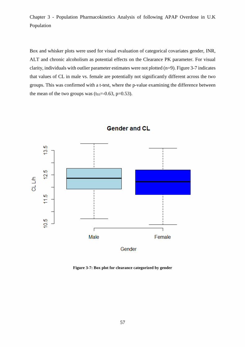
Chapter 3 - Population Pharmacokinetics Analysis of following APAP Overdose in U.K
Population
57
Box and whisker plots were used for visual evaluation of categorical covariates gender, INR,
ALT and chronic alcoholism as potential effects on the Clearance PK parameter. For visual
clarity, individuals with outlier parameter estimates were not plotted (n=9). Figure 3-7 indicates
that values of CL in male vs. female are potentially not significantly different across the two
groups. This was confirmed with a t-test, where the p-value examining the difference between
the mean of the two groups was (t93=-0.63, p=0.53).
Figure 3-7: Box plot for clearance categorized by gender
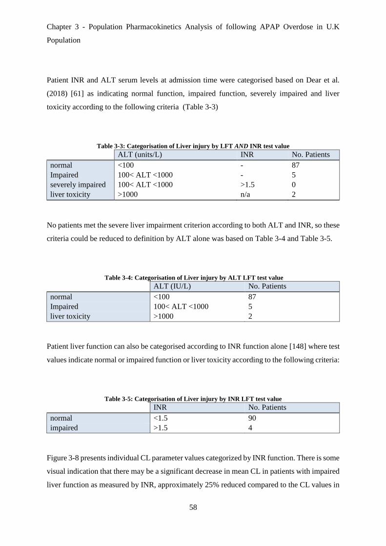
Chapter 3 - Population Pharmacokinetics Analysis of following APAP Overdose in U.K
Population
58
Patient INR and ALT serum levels at admission time were categorised based on Dear et al.
(2018) [61] as indicating normal function, impaired function, severely impaired and liver
toxicity according to the following criteria (Table 3-3)
Table 3-3: Categorisation of Liver injury by LFT AND INR test value ALT (units/L) INR No. Patients
normal <100 - 87
Impaired 100< ALT <1000 - 5
severely impaired 100< ALT <1000 >1.5 0
liver toxicity >1000 n/a 2
No patients met the severe liver impairment criterion according to both ALT and INR, so these
criteria could be reduced to definition by ALT alone was based on Table 3-4 and Table 3-5.
Table 3-4: Categorisation of Liver injury by ALT LFT test value ALT (IU/L) No. Patients
normal <100 87
Impaired 100< ALT <1000 5
liver toxicity >1000 2
Patient liver function can also be categorised according to INR function alone [148] where test
values indicate normal or impaired function or liver toxicity according to the following criteria:
Table 3-5: Categorisation of Liver injury by INR LFT test value INR No. Patients
normal <1.5 90
impaired >1.5 4
Figure 3-8 presents individual CL parameter values categorized by INR function. There is some
visual indication that there may be a significant decrease in mean CL in patients with impaired
liver function as measured by INR, approximately 25% reduced compared to the CL values in

Chapter 3 - Population Pharmacokinetics Analysis of following APAP Overdose in U.K
Population
59
the normal liver function sub-population. A t-test comparing the mean CL in the two categories
returned a p-value was (t93=-1.9, p=0.15). However, because the number of patients is minimal,
with only four patients in the impaired liver function category according to INR, out of 94, this
relationship should be treated with caution.
Figure 3-8: Box plot for clearance categorized by INR
Figure 3-9 shows the relationship of liver impairment and liver toxicity, as categorized by ALT
liver function test value to CL in this dataset. Visual inspection indicates a slight decreas in CL
in the presence of liver impairment, but increas in clearance in patients with liver toxicity.
Given the low numbers in both the impaired and liver toxicity categories however, these trends
may be artefactual and mechanistically inconsistent with each other.

Chapter 3 - Population Pharmacokinetics Analysis of following APAP Overdose in U.K
Population
60
Figure 3-9: The Boxplot shows the relation between ALT (liver impairment function and liver toxicity) on
CL.
Figure 3-10 shows individual CL parameter estimates categorized according to chronic
alcoholism status. A 13% increase in mean CL is seen in patients with chronic alcoholism
compared to those without, and this difference was shown to be significant via a t-test (t93=1.5,
p=0.04).

Chapter 3 - Population Pharmacokinetics Analysis of following APAP Overdose in U.K
Population
61
Figure 3-10: the boxplot shows the relation between chronic alcoholic patients on CL.
3.3.3.1. Covariate model runs in NONMEM
Table 3-6 shows a summary of the change in OFV under covariate models that were assessed,
where various continuous and categorical covariates were analysed for their effects on
clearance. No significant falls in OFV were seen for the continuous covariates weight and age.
For the categorical covariate for liver function based on INR (Table 3-3), NONMEM
consistently estimated a covariate effect where liver impairment patients (INR >1.5) had a
potentially lower typical CL. However, although this might make sense mechanistically,
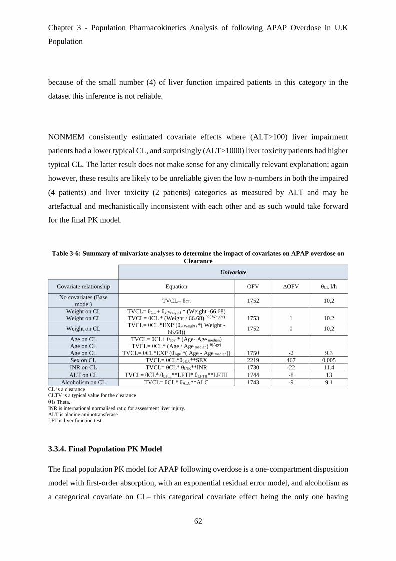
Chapter 3 - Population Pharmacokinetics Analysis of following APAP Overdose in U.K
Population
62
because of the small number (4) of liver function impaired patients in this category in the
dataset this inference is not reliable.
NONMEM consistently estimated covariate effects where (ALT>100) liver impairment
patients had a lower typical CL, and surprisingly (ALT>1000) liver toxicity patients had higher
typical CL. The latter result does not make sense for any clinically relevant explanation; again
however, these results are likely to be unreliable given the low n-numbers in both the impaired
(4 patients) and liver toxicity (2 patients) categories as measured by ALT and may be
artefactual and mechanistically inconsistent with each other and as such would take forward
for the final PK model.
Table 3-6: Summary of univariate analyses to determine the impact of covariates on APAP overdose on
Clearance
Univariate
Covariate relationship Equation OFV ΔOFV θCL l/h
No covariates (Base
model) TVCL= θCL 1752 10.2
Weight on CL TVCL= θCL + θ2(Weight) * (Weight -66.68)
Weight on CL TVCL= θCL * (Weight / 66.68) θ2( Weight) 1753 1 10.2
Weight on CL TVCL= θCL *EXP (θ2(Weight) *( Weight -
66.68)) 1752 0 10.2
Age on CL TVCL= θCL+ θcov * (Age- Age median)
Age on CL TVCL= θCL* (Age / Age median) θ(Age)
Age on CL TVCL= θCL*EXP (θAge *( Age - Age median)) 1750 -2 9.3
Sex on CL TVCL= θCL*θSEX**SEX 2219 467 0.005
INR on CL TVCL= θCL* θINR**INR 1730 -22 11.4
ALT on CL TVCL= θCL* θLFTI**LFTI* θLFTII**LFTII 1744 -8 13
Alcoholism on CL TVCL= θCL* θALC**ALC 1743 -9 9.1 CL is a clearance CLTV is a typical value for the clearance
θ is Theta.
INR is international normalised ratio for assessment liver injury.
ALT is alanine aminotransferase LFT is liver function test
3.3.4. Final Population PK Model
The final population PK model for APAP following overdose is a one-compartment disposition
model with first-order absorption, with an exponential residual error model, and alcoholism as
a categorical covariate on CL– this categorical covariate effect being the only one having

Chapter 3 - Population Pharmacokinetics Analysis of following APAP Overdose in U.K
Population
63
statistical and clinical significance, having some mechanistic rationale and having sufficient n-
numbers per category to be considered trustworthy. The final model parameter estimates are
summarised below (Table 3-7).
Diagnostic plots Figure 3-11 and Figure 3-12 indicated acceptable goodness of fit given the
limitations of the dataset (see discussion in section 3.4). Figure 3-13 presents 90% prediction
intervals and medians in the VPC are in good agreement with the observed data indicating
acceptable predictive performance of the model.
Standard errors, confidence intervals and bias for parameter estimates were calculated from
535 successful bootstrap runs with these results also summarised Table 3-7. For the fixed-
effects parameters, the bootstrap medians were very similar to the final NONMEM parameter
estimates with the original dataset, and the relative bias for CL and Vd parameters 0.8% and
7% for the alcohol covariate. The bootstrap medians for the random-effects parameters were
also in the same range of the original values with only small relative bias 0.01%.
Table 3-7 Population mean estimates of pharmacokinetic model parameters
Model Parameter Unit Base
Model
Final
Model
RSE
%
Bootstrapa
Median
Biasa Relative
Bias %a
95%
CIb
Fixed Effects
CL (L/h) 10.2 9.14 11 9.06 0.08 0.8 6-13.5
Vd (L) 133 122 12 123 1 0.8 67-218
Ka (fixed) (h) 4.57 4.57 - - - -
Covariate influence
CL_Chronic Alcoholic 0.13 - 0.14 0.01 7 0.01-0.7
Random Effect
IIV-CLc (%CVd) 43 44 26 44 0 0 17-62
Residual Error (%CV) 122 117.4 9 117.2 0.02 0.01 77-158
aobtained from 535 bootstrap runs; bias = (final model estimate – bootstrap median);
relative bias = 100 * ((final model estimate - bootstrap median) / final model estimate). bCI is Confidence Interval. cIIV-CL is inter-individual variability of clearance. dCV is a coefficient variation.

Chapter 3 - Population Pharmacokinetics Analysis of following APAP Overdose in U.K
Population
64
Figure 3-11: Goodness of fit plots for population PK final model for APAP.
LEFT: observed concentration (DV) vs. individual prediction (IPRE)
RIGHT: observed concentration (DV) vs. population prediction (PRED)
Line of unity (black) in both plots for illustration.
Figure 3-12: Residual scatter plots for population PK final model for APAP.
LEFT: conditional weighted residuals (CWRES) versus population APAP concentration prediction
RIGHT: conditional weighted residuals (CWRES) versus Time.
The VPC indicates that the description of the data by the final structural model was accurate
and precise with the 225 observed datapoints laying acceptably within 95% prediction interval
of the model.
Population APAP Concentration mg/L Prediction Time (h)
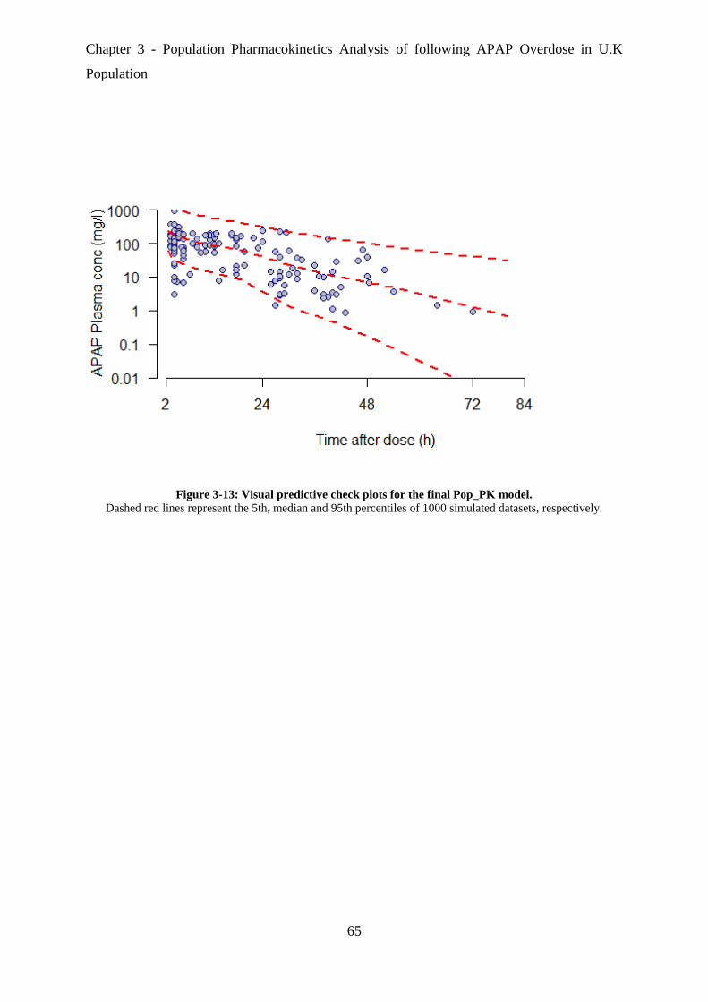
Chapter 3 - Population Pharmacokinetics Analysis of following APAP Overdose in U.K
Population
65
Figure 3-13: Visual predictive check plots for the final Pop_PK model.
Dashed red lines represent the 5th, median and 95th percentiles of 1000 simulated datasets, respectively.

Chapter 3 - Population Pharmacokinetics Analysis of following APAP Overdose in U.K
Population
66
3.4. Discussion
In reviewing the literature, no data was found describing the Pop-PK of APAP following
overdose in UK patients, and the present study was designed to address this gap in knowledge.
Earlier PK studies that involved oral dose of APAP reported a one compartment disposition
model to be most appropriate [148], and this was confirmed in the analysis of the BIOPAR
APAP overdose dataset where again a one compartment model (with first order absorption
kinetics) was chosen as the best fit for the data, however with the slight caution of the dataset
being limited to a relatively small number of patients and sparsely sampled.
The estimate of population CL in the present study (9.14 L/h) is nearly half that previously
reported for APAP by Forrest and colleagues [151] following therapeutic dose in adults (18.9-
23.1 L/h). However, the value of Vd obtained in our study (122 L) is higher than the value
reported by Levy [16] following therapeutic dose (66 L).
The current study found that the IIV of CL (expressed as a CV%) was 44%. Explanatory
covariates of age, weight, INR, ALT and alcoholism status were investigated as to their
potential to explain or predict part of the IIV on CL. This study did not find the continuous
covariates of age and weight to have a significant effect on CL. On the other hand, alcoholism
status did show a significant effect on CL, increasing the CL by approximately 14% in
alcoholics. This finding supports previous research, as alcoholism has been shown to increase
CYP2E1 expression, which is responsible for APAP metabolism. Thus, in theory, alcoholics
could remove total APAP quicker, but have a higher exposure to APAP metabolites compared
to non-alcoholics [152].
The main weakness of this study is the failure to adequately assess the effect of patients having
liver injury (as measured with LFT values of ALT>100 and INR>1.5) on their clearances of
APAP. No category of patients with liver injury showed significantly different APAP CL to
the rest of the population despite a plausible mechanistic basis for there to be some form of
Chapter 3 - Population Pharmacokinetics Analysis of following APAP Overdose in U.K
Population
67
detectable difference. A likely explanation is that the dataset was insufficiently sized and as a
result only 4 out 94 patients had increased INR and 7 out 94 had increased ALT reducing the
possibility of detecting the effect.
It is also interesting to note that the residual error estimate (under an exponential residual error
model) is high at 117.4%. The main contributor to this error is likely to be inaccurate recording
of dosing/ingestion time and amount. This key limitation to the dataset is also likely to account
for the relatively poor accounting of IIV via the random effect on CL as shown visually in
Figure 3-11 by the lack of improvement for the plot of Observed vs. Individual prediction
compared to Observed vs Population prediction (in terms of their closeness of their trends to
unity). When dose level and dose time are uncertain or inaccurate it is perhaps not unsurprising
that IIV could not be adequately partitioned from the non-predictable residual error. With this
in mind, potential future analysis might need to provide another method to account for
uncertainty in dose and dose-time (see Chapter 6).
The results of this chapter however remain important to provide the basis for the development
of PopPKPD models using a sequential approach (specifically making use of Empirical Bayes
Estimates (EBE) of individual patient PK parameter estimates) to describe the effects of APAP
overdose as measured by liver injury biomarkers as will be covered in the next chapter.

Chapter 4 –Population Pharmacokinetic /Pharmacodynamic Analysis of APAP Overdose in
U.K Population
68
Chapter-4
Population Pharmacokinetic
/Pharmacodynamic Analysis
of APAP Overdose in U.K
Population

Chapter 4 –Population Pharmacokinetic /Pharmacodynamic Analysis of APAP Overdose in
U.K Population
69
Chapter 4. Population Pharmacokinetic/Pharmacodynamic
Analysis of APAP Overdose in UK Population
4.1. Introduction
APAP overdose is considered a major medical problem in the UK and the leading cause of
drug induced liver injury and acute liver failure [2]. Stratification of risk and the need for N-
acetyl-cysteine (NAC) antidote therapy is sub-optimal and based on a timed plasma APAP
concentration based upon a nomogram treatment line approach [153]. Alanine
aminotransferase activity in serum (ALT) is widely used clinically to assess liver injury [154].
However, this biomarker is insufficient and lacks sensitivity and specificity [155]. Mechanistic
biomarkers have been demonstrated to provide added value for the early prediction of APAP-
induced hepatotoxicity [81]. Such biomarkers include: microRNA-122, HMGB1, apoptosis K-
18, necrosis K-18 and GLDH. Recent evidence from clinical and preclinical studies have
defined the development of a panel approach to determine the likelihood of liver injury, and
provide earlier detection and mechanistic understanding of prognostic information of liver
injury [156].
Further information or investigation is needed to explore the pharmacodynamic response for
these novel biomarkers. PKPD modelling is an important part of such work and allows
estimation and prediction of clinically relevant PKPD parameters to quantify and demonstrate
the dose-concentration-response relationship. When clarified, this relationship can provide,
characterise and predict information regarding the level of biomarker response followed by
ingestion of APAP overdose.
The aim of this chapter is to build population PKPD models to describe those biomarkers
predicting or influenced by liver injury followed by APAP overdose, with a specific aim to
detect the earliest biomarkers released following APAP overdose. Implementing these models
with data in a population approach allows prediction of individual parameters from otherwise

Chapter 4 –Population Pharmacokinetic /Pharmacodynamic Analysis of APAP Overdose in
U.K Population
70
sparse and/or noisy data to identify relationships between biomarker measurements and the risk
of patients suffering DILI at early hospital presentation.
4.2. Methods
4.2.1. Subjects, Sample Collection and Storage
Subjects employed in this PKPD model were recruited in the BIOPAR NHS portfolio
prospective clinical trial and were the same cohort used to develop the PK model in the previous
chapter (see section 3.2.1). Moreover, sample collection and storage were described earlier in
section (3.2.2).
4.2.2. Biomarkers Measurement
Six biomarkers were measured and used for PKPD modelling. These biomarkers were
microRNA-122, HMGB1, K-18 (i.e. apoptosis K-18 and necrosis K-18), GLDH and ALT.
4.2.2.1. microRNA-122 Measurement
microRNA-122 (miR-122) was initially extracted and purified using the commercially
available miRNeasy kit for miR-122 followed by an RNeasy MinElute Cleanup Kit which was
previously described by Lewis and colleagues [72]. 40 µg of serum was added to 200 μl
nuclease-free water and mixed with 700 μl of QIAzol reagent. It was incubated for 5 min before
the addition of 140 μl chloroform followed by centrifugation at 12,000 g at 4 oC for 15 min,
taking 350 μl of the aqueous supernatant into fresh microtubes for the QIAcube (Qiagen) to
carry out further extraction and purification automatically.
miRNAs were quantified by using a TaqMan miRNA quantitative reverse transcriptase–
polymerase chain reaction (qRT–PCR) assay according to the protocol of the manufacturer

Chapter 4 –Population Pharmacokinetic /Pharmacodynamic Analysis of APAP Overdose in
U.K Population
71
[157]. Briefly, the small RNA was reverse transcribed using specific stem-loop reverse
transcription (RT) primers; approximately 10 ng total RNA was used for first-strand cDNA
synthesis using specific primers with let7 gene expression was used as a control group. Real-
time PCR amplification was carried out with a gene-specific forwarded primer and a reverse
primer, along with a probe, in an ABI Prizm 7500 PCR machine.
4.2.2.2. HMGB1 Measurement
HMGB1 serum concentration was determined in undiluted serum using an HMGB1 enzyme-
linked immunosorbent assay (ELISA) kit, according to the guidelines of the manufacturer
[158]. The assay procedure takes two days for measurement. First day: 10 μl of both standards,
positive control and serum samples were added to the appropriate duplicate wells of a 96-well
plate followed by 100 μl of sample diluent to every well. The plate was sealed, gently shaken
and subsequently incubated at 37 oC for 20 - 24 h.
Second day: wash solution was produced by adding 100 ml wash buffer to 400 ml distilled
water (5x dilution) and each well was washed five times with 400 μl/well and the plate dried
manually. 100 μl of the enzyme conjugate solution was then added followed by sealing the
plate and incubation at 25 C for 2 hrs. The plate was then washed again followed by addition
of substrate solutions A and B mixed in equal parts, adding 100 μl of this substrate solution
mix to each well, followed by incubation in darkness and at room temperature for a further 30
min, then added of 100 μl of stop solution. Five minutes later, the plate was read at 450 nm
using a Varioskan Flash machine [159] to assess colour intensity for HMGB1 measurement.
The lower limit of quantification (LLQ) was 0.1 ng/ml.
4.2.2.3. K-18 Measurement
Quantitative detection of apoptosis K-18 biomarker was determined by using ELISA assays
for epithelial keratin M30 (apoptosense) [160], and necrosis K1-8 biomarker by epithelial
Chapter 4 –Population Pharmacokinetic /Pharmacodynamic Analysis of APAP Overdose in
U.K Population
72
keratin M65 (EpiDeath) [161] according to the manufacturer’s guidelines. The M30 antibody
specifically binds caspase-cleaved keratin 18 but does not bind the un-cleaved form, and M65
is used for determination of total cell death in the study of epithelial cells.
25 μl of standards, controls (low and high) and serum samples were mixed into 96-well plates
in appropriate duplicate wells. 75 μl of the conjugate solution was then added to every well and
the plate sealed and incubated for 2 hrs (M65) or 4 hrs (M30) on a plate shaker at 600 rpm.
Then the plate was washed out manually with 250 μl wash solution per well and the plate dried.
200 μl of substrate solution was then added to each well and the plate was incubated in darkness
at room temperature for 20 min. After the incubation period, 50 μl of stop solution was added
and the plate was shaken. Lastly, after 5 - 30 min the absorbance at 450 nm was read using a
Varioskan Flash machine [159].
4.2.2.4. GLDH Measurement
Glutamate dehydrogenase (GLDH) activity was measured by using a kinetic assay in a 96-well
plate format. Briefly, to each well was added: 150 l 75 mM triethanolamine and ammonium
sulfate buffer, 5 l 11 mM NADH, 20 l 14.2 mM ADP and 60 l serum (or diluted
serum). Plate contents were mixed and incubated at 37C for 15 minutes. The reaction was
initiated by addition of 65l of 45 M -ketoglutaric acid. The contents of the well were mixed,
and the change in absorbance (340nm) was measured over 5 minutes. The rate of fall in
E340/min was converted to International Units per litre (U/l).
4.2.2.5. ALT Measurement
Serum Alanine transaminase (ALT) was measured with a photometric kinetic assay, by using
InfinityTM ALT (GPT) Liquid Stable Reagent according to the guidelines of the manufacturer
[162]. 30 μl of sample was loaded in duplicate into 96-well plates. Then mixed with 300 μl of
ALT reagent per well to each sample before assaying on a Varioskan Flash machine [159].

Chapter 4 –Population Pharmacokinetic /Pharmacodynamic Analysis of APAP Overdose in
U.K Population
73
There is a series of reactions involved in the assay system leading to a reduction of pyruvate to
L-lactate with lactate dehydrogenase as a result of the oxidisation of NADH to NAD. The
oxidation of NADH leads to a decrease in absorbance at 340 nm, and ALT activity is therefore
assayed by calculating the maximum rate of change in this absorbance over multiple readings.
4.2.3. Population Pharmacokinetics Pharmacodynamics Models
Mechanism-based pharmacokinetic-pharmacodynamic modelling (PKPD) aims to predict
exposure-response relationships, especially in vivo, and can also be used to characterise the
interaction of drug effect with disease processes or progression [163]. The concept of
mechanism-based modelling of PKPD is enhanced in often novel dimensions by the selection,
evaluation and validation of biomarkers with strong emphasis on mechanistic rationale [164].
Biomarkers in this context are defined as the means to quantify a relationship between drug
exposure and effect. In 2005, Danhof and colleagues classified seven main types of biomarker
based on mechanism and location (Table 4-1). In this thesis, types 4 was used to quantify the
APAP dose-concentration-response relationship and thus eventually to provide information for
prediction of the level of acute liver injury given a certain level of APAP dose.
Table 4-1: The Mechanistic Classification of Biomarkers[165]
Type 0: Genotype or Phenotype
Type 1: Concentration of drug or metabolite
Type 2: Target occupancy
Type 3: Target activation
Type 4: Physiological measure or laboratory test
Type 5: Disease Processes
Type 6: Clinical Scales
Population PKPD modelling uses statistical models to describe observations of concentrations
and effects and their variability but may also give some insight into the underlying biological
process. Variability in plasma concentrations between-subjects also often tends to be lower
than in effects and a Pop-PKPD approach can allow the characterisation of both sources of
variability.
Chapter 4 –Population Pharmacokinetic /Pharmacodynamic Analysis of APAP Overdose in
U.K Population
74
4.2.4. NLME Structural and Statistical Model Development
After a dose of APAP, changes in concentration and effect will occur over time, and a basic
PKPD model using a direct effect between plasma concentration and the observed
biomarker/effect/outcome may be unable to explain the concentration-effect relationship due
to delays in response.
This phenomenon has been shown previously for APAP where a PD model for the
concentration effect relationship of APAP (and hence its dose-response) was described by Gibb
and Anderson [166] for outcome biomarkers such as pain score and temperature following a
therapeutic dose. It was shown in a plot of effect vs. concentration with observations labelled
in chronological order that a hysteresis loop was present, resulting from a delay in effect. A
hypothetical effect compartment model was thus used in their PKPD analysis.
The effect compartment model as described previously (section 2.1.2.2) is one theoretical
concept to overcome the issue of delay in response from a given driving PK concentration, and
describes a compartment offset by a delay/activation/deactivation parameter (Ke0) from the
driving PK concentration compartment(Figure 4-1).

Chapter 4 –Population Pharmacokinetic /Pharmacodynamic Analysis of APAP Overdose in
U.K Population
75
Figure 4-1: Schematic description of effect compartment model
It was initially assumed that given an effect compartment model was shown to be sufficient to
describe a therapeutic APAP dose effect by Gibb and Anderson that the same model could be
applied to data following overdose in this thesis. However, preliminary analysis of the
biomarker data using this form of PKPD model found that applying the approach of Gibb and
Anderson was not appropriate. Despite various attempts adjusting various NONMEM options
(e.g. initial parameter estimates, estimation method, significant figures of the estimation, type
of ODE solver, etc.) no analytical runs for the biomarker data using this model were successful
– consistently failing to minimise successfully and give parameter estimates. There are several
potential reasons for this including:

Chapter 4 –Population Pharmacokinetic /Pharmacodynamic Analysis of APAP Overdose in
U.K Population
76
The much higher APAP doses (i.e. overdose above 4g of single acute doe) in this data
compared to the data of Gibb et al. with the resultant higher modelled PK concentrations
giving a potential PD response to a different order of magnitude to the previous data.
That the BIOPAR biomarker data was of target effect biomarkers as opposed to the
outcome biomarkers (e.g. reduction in fever, pain score) used by Gibb and Anderson
which may have a qualitatively different behaviour in terms of noise, influence by other
physiological factors etc.
That the time course of effect of the biomarkers in this dataset was more clearly
described as a deviation from, followed by a return to, baseline which may have been
less easily described or parameterised with solely an effect compartment model.
Preliminary analytical efforts then moved on to applying an indirect response model to the
biomarker data (section 2.1.2.3) however these attempts also failed to fit the data, likely for
similar reasons to the effect compartment model. As a result, an approach was adopted where
an indirect response model was combined in sequence with the effect compartment model to
sufficiently account for the apparent delays in response and the nature of the data describing
APAP overdose effects in the data being analysed.
4.2.4.1. Sequential effect compartment / indirect response model
As previously described (section 2.1.2.3) indirect response PD models were developed to
describe drug effects where pharmacological actions occur by indirect mechanisms such as
inhibition or stimulation of the production or dissipation of factors resulting in the measured
effect. They have been previously implemented in sequence with a delay/effect compartment,
for example in the work of Cleton et al. [167].
The sequential effect compartment/indirect response PKPD model for APAP is described by
four compartments. These compartments are gut, central, effect and response. Figure 4-3: The

Chapter 4 –Population Pharmacokinetic /Pharmacodynamic Analysis of APAP Overdose in
U.K Population
77
descriptive assumption of compartment models location related to APAP metabolism.Figure
4-3 below represents these four compartments. Gut and central compartments are the one-
compartment oral PK disposition model for APAP, the effect and indirect response
compartments are the PD model to describe APAP effects.
Figure 4-2: First Order Kinetic Combined with Effect Compartment followed by Indirect Response
The ordinary differential equations for gut, central, effect and response compartments in the
schematic are outlined below in, Equation 4-1, Equation 4-2, Equation 4-3, Equation 4-4 and
Equation 4-5, respectively. Cp is the plasma concentration, and Kel is the first order elimination
rate constant of the drug equal to Clearance divided by Volume of distribution. E is the
magnitude of the effect driven by the Effect compartment concentration which is a function of
the effect compartment “concentration” (Ce) using the previously described Emax model

Chapter 4 –Population Pharmacokinetic /Pharmacodynamic Analysis of APAP Overdose in
U.K Population
78
(Equation 2-5). This drug effect magnitude then acts on the Kout “dissipation” parameter of
the indirect response model (i.e. the form of indirect response model in Equation 2-16). The
value of the response compartment is then used to model the observed drug
response/effect/biomarker data.
dDepot/dt = -Ka * Depot Equation 4-1
dCp/dt = Ka*Depot/V – Kel * Cp Equation 4-2
dCe/dt = Ke0 * Cp– Ke0 * Ce Equation 4-3
E = (Emax*Ce)/(EC50+Ce) Equation 4-4
dResponse/dt = Kin-Kout*(1-E)* Response Equation 4-5
During preliminary analyses model fitting attempts were made using the other forms of indirect
response PD models, with drug effect manifested as stimulation or inhibition of Kin or Kout.
(i.e. exploration of alternate versions of Equation 4-5 based on the alternate forms of indirect
response model as outlined in 2.1.2.3). However, these efforts failed to minimise successfully
in fitting the data and Equation 4-5 was the final form used for the BIOPAR data analysis.
When drug concentration equals zero, E = 0 and then Equation 4-7 becomes Equation 4-6.
dResponse/dt = Kin – Kout * Response Equation 4-6
When the drug concentration equals zero then response is presumed to be at its steady state
value E0, with its rate of change assumed to be zero. Equation 4-6 can then be manipulated via

Chapter 4 –Population Pharmacokinetic /Pharmacodynamic Analysis of APAP Overdose in
U.K Population
79
Equation 4-7 and Equation 4-8 into Equation 4-9. In the absence of drug therefore the steady
state value of the response is given by Kin/Kout, and this can be used as the baseline, initial
condition at time = 0, for the response being modelled, when no drug is present in the system.
0 = Kin – Kout * Response Equation 4-7
Kout * Response = Kin Equation 4-8
Response = Kin / Kout = E0 (at steady state) Equation 4-9
It should also be noted that a half-life for observed biomarker response can be given by
Equation 4-10:
T1/2 Response = ln(2) / Kout Equation 4-10
Further, the trapezoid method was used to calculate AUCbiomarkers. Equation 4-11
AUCbiomarker = (Tb – Ta) *(Cb + Ca)/2 Equation 4-11
Figure 4-3 shows how the sequential effect compartment/indirect response model could be
rationalised mechanistically with the metabolism of APAP into NAPQI that is then detoxified
with glutathione [168]. The increased production of NAPQI under overdose leads to APAP
adduct production, toxic effects and changes in the observed biomarkers [169]. These effects
would require an extra process and delay to be modelled that would not occur following a
therapeutic APAP dose, which may explain the need for the addition of an indirect response
model in sequence to an effect compartment for these biomarkers, as opposed to the outcome
biomarkers previously modelled for APAP effect under therapeutic doses.

Chapter 4 –Population Pharmacokinetic /Pharmacodynamic Analysis of APAP Overdose in
U.K Population
80
Figure 4-3: The descriptive assumption of compartment models location related to APAP metabolism.
4.2.5. NLME analysis of APAP overdose biomarker data
Analysis of the APAP overdose biomarker data was carried out with a population approach in
NONMEM as for the APAP PK concentration data in chapter 3. The method and approach is
largely as previously described, including the approach taken with outlier data points. As for
the final PK an exponential residual error model was applied with the data for each biomarker.
The PKPD structural models were implemented in NONMEM as differential equations using
the general differential equation solvers of either ADVAN 6, 8 or 13 of the NONMEM
PREDPP subroutines library. The same differential equation model solver subroutine was not
applicable for the analysis of all the different biomarker: ADVAN 6, which uses a general non-
stiff numerical ordinary differential equation solver, was unable to minimise successfully with
some analyses and for these the alternative stiff differential equation solvers in ADVAN 8 or

Chapter 4 –Population Pharmacokinetic /Pharmacodynamic Analysis of APAP Overdose in
U.K Population
81
13 were used as necessary. In addition, for reasons of stability, the initial condition of the
response (E0, Equation 4-12) was estimated as a parameter in NONMEM and then Kout
calculated for the PD differential equation model using E0 combined with the estimate of Kin
as per Equation 4-12.
The PKPD data analysis was performed sequentially, where the pharmacokinetic parameters
were first estimated in the subject population with the previously specified PK model (section
3.2.5) for APAP overdose. Then the PD model for the biomarker was fitted to the population
biomarker data, having fixed each individual subject’s PK parameters to their individual
estimates from the first-stage population PK fitting. Pop-PKPD models therefore allow the
incorporation of PK variability, but are then able to include further characterisation of
variability in effect.
With the final model fitting to the data in place, individual pharmacokinetic and
pharmacodynamic parameter estimates for each patient obtained from the final Pop-PKPD
model were used to simulate rich time-courses of APAP concentrations and biomarkers over
384 hours to give a precise description of the time course of effect to reach the true expected
peak value. This description can give an indication of the potential value of the biomarkers in
early detection of liver injury and a modelled estimate of the peak value and the time it occurs
for those biomarkers.

Chapter 4 –Population Pharmacokinetic /Pharmacodynamic Analysis of APAP Overdose in
U.K Population
82
4.3. Results
4.3.1. Data
Demographic data was as described previously in (Section 3.3.1). As described previously the
median APAP ingestion in the overdose patients was 32g (range 8-140g), the median time
delay between the time of APAP ingestion and a first blood sample was approximately 5 h
(range 2-72h). Table 4-2 below presents a breakdown of the serum levels of ALT and novel
biomarkers, as measured upon admission to hospital, and number of patients within each
category.
Table 4-2: Clinical Biomarkers Measurements at the First Presentation to the Hospital.
Biomarkers
Admission Serum
Level (Median,
Range)
No. of Patients within the
average values** (%)
No. of Patients above average
values (%)
ALT
20 IU/L
(9-1790)
78 (83%)
< 50 IU/L
16 (17%)
> 50 IU/L
HMGB1
1.1 ng/ml
(0.17-47)
75 (79%)
< 2.4 ng/ml
19 (21%)
> 2.4 ng/ml
miR-122
0.3 6 Let-7d
normalized
(0.1-5337)
77 (82%)
< 6 Let-7d normalized
17 (18%)
> 6 Let-7d normalized
GLDH
16 IU/L
(5-9389)
78 (83%)
<30 IU/L
16 (17%)
> 30 IU/L
Apoptosis K-18
199 IU/L
(108-8941)
70 (74%)
< 291 IU/L
24 (26%)
> 291 IU/L
Necrosis K-18
321 IU/L
(112-12547)
21 (19%)
<197 IU/L
73
(81%) >197 IU/L
IU - International Unit **Average value see Table 1-1
4.3.2. HMGB1 PKPD Analysis
218 serum blood samples collected from 94 subjects were available for Pop-PKPD analysis for
the HMGB1 biomarker with a minimum of 2 samples at different time points per patient.
Parameter estimates of the Pop-PKPD model fit to the HMGB1 biomarker data using the

Chapter 4 –Population Pharmacokinetic /Pharmacodynamic Analysis of APAP Overdose in
U.K Population
83
ADVAN13 subroutine are summarised in Table 4-3. The population mean estimate for E0
(baseline of observed HMGB1) was 1.14 ng/ml, which is within the normal range of human
HMGB1 activity (0.17 – 2.42 ng/ml). The maximum predicted response after APAP overdose
(as given by Emax) was an inhibition of 102% in the Kout dissipation parameter of the indirect
effect PD model. The estimated IIV for each structural model parameter, as well as the residual
error component of the model, was high and likely reflects the noisy and sparse nature of the
data where there was significant variability between patients in response to APAP induced liver
injury.
Table 4-3: Population Mean Estimates of HMGB1 Pharmacodynamic Model Parameters
Model Parameter Unit Final
Model
RSE%a Bootstrapb
Median
Biasb Relative
Bias%b
95% CIc
Fixed Effects
KE0 (h) 0.5 10 0.5 0 0 0.3-0.7
KIN (h) 0.001 0.68 0.001 0 0 0.0006-0.003
E0 (U/L) 1.14 46 1.12 0.02 2.04 0.99-1.29
EMAX (%) 102 49 100 2 2.8 58-310
EC50 (mg/l) 0.32 59 1.02 0.7 1.4 0.15-0.45
Random Effect
IIVd_KE0 (%CVe) 26 33 24 9 -10 20-47
IIVd_KIN (%CVe) 30 0.74 30 0 0 2-38
IIVd_E0 (%CVe) 70 38 70 0 0 47-77
IIVd_EMAX (%CVe) 28 39 24 4 14 2-31
IIVd_EC50 (%CVe) 10 3.9 70 0 0 4-14
Residual Error (%CVd) 50 23 50 0 0 45-55 aRSE; relative standard error = (standard error/final estimation)*100 bobtained from 374 bootstrap runs; bias = (final model estimate – bootstrap median); relative bias = 100 * ((final model estimate - bootstrap median) / final model estimate). cCI is Confidence Interval. dIIV is inter-individual variability of clearance. eCV is a coefficient variation.

Chapter 4 –Population Pharmacokinetic /Pharmacodynamic Analysis of APAP Overdose in
U.K Population
84
4.3.2.1. Model evaluation
Goodness-of-fit of the HMGB1 PKPD model was assessed by a graphical approach (Figure
4-4). The plot of observed biomarker values vs. individual PKPD model predictions indicates
that the model predicted biomarker levels agreed satisfactorily with observed concentrations.
However, the plot of observed biomarker values vs. population PKPD model predictions looks
more unusual, but this can be attributed to the small range in the individual PK parameter
estimates for each subject in this dataset (i.e. because this is a 2-stage analysis, the population
predictions shown in this plot reflect the population fixed effects PD estimates, combined with
a small range in individual PK parameter values). The plots of CWRES vs. time or individual
predicted values are randomly scattered around zero across their ranges suggesting minimal
bias or trends in the residual error model (Figure 4-5).
A VPC of how the final HMGB1 Pop-PKPD model predicts the observed HMGB1 biomarker
values was produced from 1000 simulated replicates of the study dataset using the population
estimates of the model parameters and their variabilities. Observations mainly lie within the
90% prediction interval and the extremes of the 90% prediction interval reflect the 5th and 95th
percentiles of the observed data (Figure 4-6).
A non-parametric bootstrap was also used to evaluate the model and as internal validation for
the fitting. The bootstrap estimates (summarised inTable 4-3) were reasonably close to those
gained from the final NONMEM minimisation (within 10% difference) with the estimates
contained within the 95% confidence intervals gained from bootstrap suggesting that the fitting
is reliable.

Chapter 4 –Population Pharmacokinetic /Pharmacodynamic Analysis of APAP Overdose in
U.K Population
85
Figure 4-4: Goodness of fit plots for population PKPD base model for HMGB1.
LEFT: observed concentration (DV) vs. individual prediction (IPRE)
RIGHT: observed concentration (DV) vs. population prediction (PRED)
Line of unity (black) in both plots for illustration.
Figure 4-5: Residual scatter plots for population PKPD base model for HMGB1.
LEFT: conditional weighted residuals (CWRES) versus individual HMGB1 concentration prediction
RIGHT: conditional weighted residuals (CWRES) versus Time
R2 = 0.657

Chapter 4 –Population Pharmacokinetic /Pharmacodynamic Analysis of APAP Overdose in
U.K Population
86
Figure 4-6: Visual predictive check plots for the final HMGB1 Pop_PKPD model.
Dashed red lines represent the 5th, median and 95th percentiles of 1000 simulated datasets, respectively
4.3.2.2. HMGB1 peak response and predicted half-life
Below is a summary of observed and predicted time of peak response (Tmax), peak response
and half-life estimate for the HMGB1 biomarker (Table 4-4):
Table 4-4: Peak and time of HMGB1 response after APAP overdose and half life
Time of Peak Response(h) Peak Response (IU/l) Half Life (h)*
HMGB1 Observed Model Observed Model
169 128 10 3.5 940 *Half-life (h1/2)=In(2)/Kout
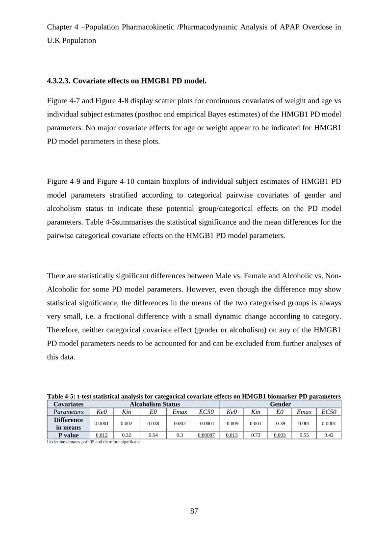
Chapter 4 –Population Pharmacokinetic /Pharmacodynamic Analysis of APAP Overdose in
U.K Population
87
4.3.2.3. Covariate effects on HMGB1 PD model.
Figure 4-7 and Figure 4-8 display scatter plots for continuous covariates of weight and age vs
individual subject estimates (posthoc and empirical Bayes estimates) of the HMGB1 PD model
parameters. No major covariate effects for age or weight appear to be indicated for HMGB1
PD model parameters in these plots.
Figure 4-9 and Figure 4-10 contain boxplots of individual subject estimates of HMGB1 PD
model parameters stratified according to categorical pairwise covariates of gender and
alcoholism status to indicate these potential group/categorical effects on the PD model
parameters. Table 4-5summarises the statistical significance and the mean differences for the
pairwise categorical covariate effects on the HMGB1 PD model parameters.
There are statistically significant differences between Male vs. Female and Alcoholic vs. Non-
Alcoholic for some PD model parameters. However, even though the difference may show
statistical significance, the differences in the means of the two categorised groups is always
very small, i.e. a fractional difference with a small dynamic change according to category.
Therefore, neither categorical covariate effect (gender or alcoholism) on any of the HMGB1
PD model parameters needs to be accounted for and can be excluded from further analyses of
this data.
Table 4-5: t-test statistical analysis for categorical covariate effects on HMGB1 biomarker PD parameters
Covariates Alcoholism Status Gender
Parameters Ke0 Kin E0 Emax EC50 Ke0 Kin E0 Emax EC50
Difference
in means 0.0001 0.002 0.038 0.002 -0.0001 -0.009 0.001 -0.39 0.001 0.0001
P value 0.012 0.32 0.54 0.3 0.00007 0.013 0.73 0.003 0.55 0.42
Underline denotes p<0.05 and therefore significant

Chapter 4 –Population Pharmacokinetic /Pharmacodynamic Analysis of APAP Overdose in
U.K Population
88
Figure 4-7: Scatter plots for age covariate relationship with HMGB1 dynamic parameters.

Chapter 4 –Population Pharmacokinetic /Pharmacodynamic Analysis of APAP Overdose in
U.K Population
89
Figure 4-8: Scatter plots for weight covariate relationship with HMGB1 dynamic parameters.

Chapter 4 –Population Pharmacokinetic /Pharmacodynamic Analysis of APAP Overdose in
U.K Population
90
Figure 4-9: Boxplots of HMGB1 pharmacodynamic model parameters categorized by gender.
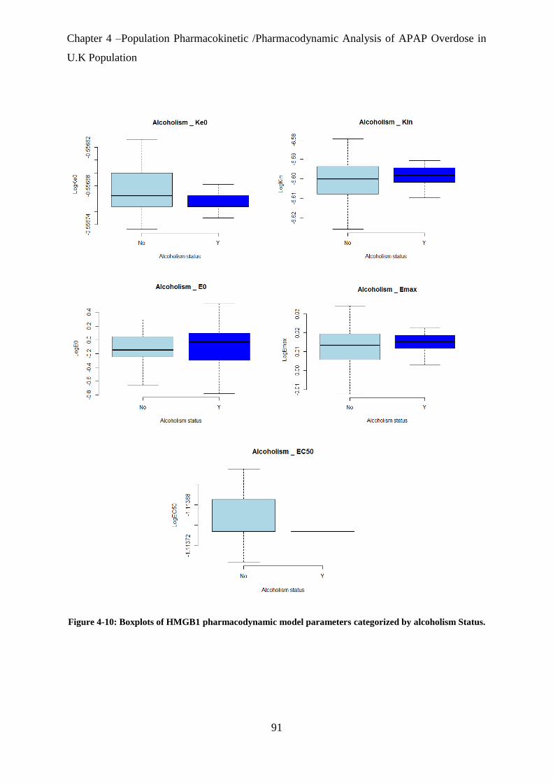
Chapter 4 –Population Pharmacokinetic /Pharmacodynamic Analysis of APAP Overdose in
U.K Population
91
Figure 4-10: Boxplots of HMGB1 pharmacodynamic model parameters categorized by alcoholism Status.

Chapter 4 –Population Pharmacokinetic /Pharmacodynamic Analysis of APAP Overdose in
U.K Population
92
4.3.3. miR-122 PKPD Analysis
229 serum blood samples collected from 94 subjects were available for Pop-PKPD analysis for
the miR-122 biomarker. Parameter estimates of the Pop-PKPD model fit to the miR-122
biomarker data using the ADVAN13 subroutine are summarised in Table 4-6. The population
mean estimate for E0 (baseline of observed miR-122) was 0.57 Let-7dnormalized, which is
within the normal range of miR-122 activity (0.17 – 6 Let-7dnormalized). The maximum
predicted response after APAP overdose (as given by Emax) was an inhibition of 36% in the
Kout dissipation parameter of the indirect effect PD model. The estimated IIV for each
structural model parameter, as well as the residual error component of the model, was high and
likely reflects the noisy and sparse nature of the data where there was significant variability
between patients in response to APAP induced liver injury.
Table 4-6: Population Mean Estimates of miR-122 Pharmacodynamic Model Parameters
Model
Parameter
Unit Final
Model
RSE%a Bootstrapb
Median
Biasb Relative
Bias %b
95% CIc
Fixed Effects KE0 (h) 0.01 78 0.01 0 0 0.007-0.03
KIN (h) 0.1 90 0.09 0.01 10 0.06-0.24
E0 (Let-
7dnormalized)
0.57 26 0.52 0.05 8 0.2-0.7
EMAX (%) 36 27 33 3 8 12-72
EC50 (mg/L) 1.81 34 1.71 0.1 5 0.6-3.1
Random Effect
IIVd_KE0 (%CVe) 14 45 14 0 0 7-17
IIVd_KIN (%CVe) 14 50 14 0 0 9-20
IIVd_E0 (%CVe) 130 25 133 -3 -2 85-175
IIVd_EMAX (%CVe) 89 55 95 6 6 44-134
IIVd_EC50 (%CVe) 45 30 45 0 0 17-70
Residual Error (%CVe) 89 10 89 0 0 28-132
aRES; relative standard error = (standard error/final estimation)*100 bobtained from 302 bootstrap runs; bias = (final model estimate – bootstrap median);
relative bias = 100 * ((final model estimate - bootstrap median) / final model estimate). cCI is Confidence Interval. dIIV is inter-individual variability of clearance. eCV is a coefficient variation.

Chapter 4 –Population Pharmacokinetic /Pharmacodynamic Analysis of APAP Overdose in
U.K Population
93
4.3.3.1. Model evaluation
Goodness-of-fit of the miR-122 PKPD model was assessed by a graphical approach (Figure
4-11). The plot of observed biomarker values vs. individual PKPD model predictions indicates
that the model predicted biomarker levels did not agree ideally with observed biomarker
concentrations, however this fitting represents the best that was achievable with this data. The
plot of observed biomarker values vs. population PKPD model predictions looks more unusual,
but again this can be attributed to the small range in the individual PK parameter estimates for
each subject in this dataset (i.e. because this is a 2-stage analysis, the population predictions
shown in this plot reflect the population fixed effects PD estimates, combined with a small
range in individual PK parameter values). The plot of CWRES vs. time shows a random scatter
around zero across its range, while CWRES vs. individual predicted values shows a random
scatter around zero for lower concentrations, but a trend for positive residuals at higher levels
of the biomarker suggesting some degree of under prediction by the model fitting at these
higher levels, but overall relatively acceptable bias or trends in the residual error model (Figure
4-12). The residual pattern and nature of the model fit may also reflect the relative lack of
samples with high biomarker concentrations in the dataset meaning there is less information in
the data in order for the fitting to describe them well.
A VPC of how the final miR-122 Pop-PKPD model predicts the observed miR-122 biomarker
values was produced from 1000 simulated replicates of the study dataset using the population
estimates of the model parameters and their variabilities. Observations mainly lie within the
90% prediction interval and the extremes of the 90% prediction interval reflect the 5th and 95th
percentiles of the observed data (Figure 4-13).
A non-parametric bootstrap was also used to evaluate the model and as internal validation for
the fitting. The bootstrap estimates (summarised in Table 4-6) were reasonably close to those
gained from the final NONMEM minimisation, (within 10% difference) with the estimates
contained within the 95% confidence intervals gained from bootstrap suggesting that the fitting
is reliable.

Chapter 4 –Population Pharmacokinetic /Pharmacodynamic Analysis of APAP Overdose in
U.K Population
94
Figure 4-11: Goodness of fit plots for population PKPD base model for miR-122.
LEFT: observed concentration (DV) vs. individual prediction (IPRE)
RIGHT: observed concentration (DV) vs. population prediction (PRED)
Line of unity (black) in both plots for illustration.
Figure 4-12: Residual scatter plots for population PKPD base model for miR-122.
LEFT: conditional weighted residuals (CWRES) versus individual miR-122 concentration prediction
RIGHT: conditional weighted residuals (CWRES) versus time.
R2=0.64

Chapter 4 –Population Pharmacokinetic /Pharmacodynamic Analysis of APAP Overdose in
U.K Population
95
Figure 4-13: Visual predictive check plots for the final miR-122 Pop-PKPD model.
Dashed red lines represent the 5th, median and 95th percentiles of 1000 simulated datasets, respectively.
4.3.3.2. miR-122 peak response and predicted half-life
Below is a summary of observed and predicted Tmax and peak response for the miR-122
biomarker (Table 4-7):
Table 4-7: Peak and time of miR-122 response after APAP overdose and half-life.
Time of Peak Response(h) Peak Response (IU/l) Half Life (h)*
miR-122 Observed Model Observed Model 121
144 70 110 25 *Half-life (h1/2)=In(2)/Kout
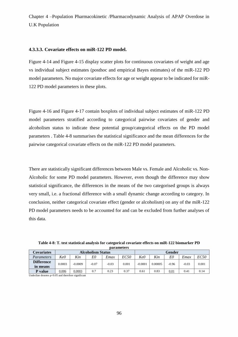
Chapter 4 –Population Pharmacokinetic /Pharmacodynamic Analysis of APAP Overdose in
U.K Population
96
4.3.3.3. Covariate effects on miR-122 PD model.
Figure 4-14 and Figure 4-15 display scatter plots for continuous covariates of weight and age
vs individual subject estimates (posthoc and empirical Bayes estimates) of the miR-122 PD
model parameters. No major covariate effects for age or weight appear to be indicated for miR-
122 PD model parameters in these plots.
Figure 4-16 and Figure 4-17 contain boxplots of individual subject estimates of miR-122 PD
model parameters stratified according to categorical pairwise covariates of gender and
alcoholism status to indicate these potential group/categorical effects on the PD model
parameters . Table 4-8 summarises the statistical significance and the mean differences for the
pairwise categorical covariate effects on the miR-122 PD model parameters.
There are statistically significant differences between Male vs. Female and Alcoholic vs. Non-
Alcoholic for some PD model parameters. However, even though the difference may show
statistical significance, the differences in the means of the two categorised groups is always
very small, i.e. a fractional difference with a small dynamic change according to category. In
conclusion, neither categorical covariate effect (gender or alcoholism) on any of the miR-122
PD model parameters needs to be accounted for and can be excluded from further analyses of
this data.
Table 4-8: T. test statistical analysis for categorical covariate effects on miR-122 biomarker PD
parameters
Covariates Alcoholism Status Gender
Parameters Ke0 Kin E0 Emax EC50 Ke0 Kin E0 Emax EC50
Difference
in means 0.0003 -0.0009 -0.07 -0.03 0.001 -0.0001 0.00005 -0.96 -0.03 0.001
P value 0.006 0.0003 0.7 0.23 0.37 0.61 0.83 0.01 0.41 0.14
Underline denotes p<0.05 and therefore significant

Chapter 4 –Population Pharmacokinetic /Pharmacodynamic Analysis of APAP Overdose in
U.K Population
97
Figure 4-14: Scatter plots for age covariate relationship with miR-122 dynamic parameters.

Chapter 4 –Population Pharmacokinetic /Pharmacodynamic Analysis of APAP Overdose in
U.K Population
98
Figure 4-15: Scatter plots for weight covariate relationship with miR-122 dynamic parameters.

Chapter 4 –Population Pharmacokinetic /Pharmacodynamic Analysis of APAP Overdose in
U.K Population
99
Figure 4-16: Boxplots of miR-122 pharmacodynamic model parameters categorized by gender.

Chapter 4 –Population Pharmacokinetic /Pharmacodynamic Analysis of APAP Overdose in
U.K Population
100
Figure 4-17: Boxplots of miR-122 pharmacodynamic model parameters categorized by Alcoholism Status.

Chapter 4 –Population Pharmacokinetic /Pharmacodynamic Analysis of APAP Overdose in
U.K Population
101
4.3.4. GLDH PKPD Analysis
208 serum blood samples collected from 94 subjects were available for Pop-PKPD analysis for
the GLDH biomarker with a minimum of 2 samples at different time points per patient.
Parameter estimates of the Pop-PKPD model fit to the GLDH biomarker data using the
ADVAN 13 subroutine are summarised in (Table 4-9). The population mean estimate for E0
(baseline of observed GLDH) was 15.1 U/L, which is within the normal range of human GLDH
activity (0.3-30 U/L). The maximum predicted response after APAP overdose (as given by
Emax) was an inhibiton of 105% in the Kout dissipation parameter of the indirect effect PD
model. The estimated IIV for each structural model parameter, as well as the residual error
component of the model, was high and likely reflects the noisy and sparse nature of the data
where there was significant variability between patients in response to APAP induced liver
injury.
Table 4-9: Population Mean Estimates of GLDH Pharmacodynamic Model Parameters
Model Parameter Unit PD
Estimation
RSEa% Bootstrapb
Median
Biasb Relative
Bias%b
95% CIc
Fixed Effects KE0 (h) 0.06 50 0.051 0.009 15 0.04-0.08
KIN (h) 0.05 63 0.04 0.01 20 0.008-0.06
E0 (U/l) 15.1 7.6 14.4 0.6 4 12-16
EMAX (%) 105 54 101 4 3.8 75-135
EC50 (mg/l) 0.53 49 0.5 0.03 6 0.1-0.99
Random Effect
IIVd_KE0 (%CVe) 88 51 97 -9 -10 20-154
IIVd_KIN (%CVe) 56 43 61 -5 -8 12-100
IIVd_E0 (%CVe) 88 49 71 17 19 24-152
IIVd_EMAX (%CVe) 32 53 37 -5 -15 10-54
IIVd_EC50 (%CVe) 33 42 32 1 3 8-58
Residual Error (%CVe) 46 14.9 45 1 2 31-54
aRSE; relative standard error = (standard error/final estimation)*100 bobtained from 463 bootstrap runs; bias = (final model estimate – bootstrap median); relative bias = 100 * ((final model estimate - bootstrap median) / final model estimate). cCI is Confidence Interval. dIIV is inter-individual variability of clearance. eCV is a coefficient variation

Chapter 4 –Population Pharmacokinetic /Pharmacodynamic Analysis of APAP Overdose in
U.K Population
102
4.3.4.1. Model evaluation
Goodness-of-fit of the GLDH PKPD model was assessed by a graphical approach (Figure
4-25). The plot of observed biomarker values vs. individual PKPD model predictions indicates
that the model predicted biomarker levels agreed well with observed concentrations. Once
again however, the plot of observed biomarker values vs. population PKPD model predictions
looks unusual, but can be attributed to the small range in the individual PK parameter estimates
for each subject in this dataset combined with this being a sequential PK-PD analysis. The plots
of CWRES vs. time or individual predicted values are randomly scattered around zero across
their ranges suggesting minimal bias or trends in the residual error model (Figure 4-19).
A VPC of how the final GLDH Pop-PKPD model predicts the observed GLDH biomarker
values was produced from 1000 simulated replicates of the study dataset using the population
estimates of the model parameters and their variabilities. Observations mainly lie within the
90% prediction interval and the extremes of the 90% prediction interval reflect the 5th and 95th
percentiles of the observed data (Figure 4-20).
A non-parametric bootstrap was also used to evaluate the model and as internal validation for
the fitting. The bootstrap estimates (summarised in Table 4-9) were reasonably close to those
gained from the final NONMEM minimisation, (within 10% difference) with the estimates
contained within the 95% confidence intervals gained from bootstrap suggesting that the fitting
is reliable.

Chapter 4 –Population Pharmacokinetic /Pharmacodynamic Analysis of APAP Overdose in
U.K Population
103
Figure 4-18: Goodness of fit plots for population PKPD base model for GLDH.
LEFT: observed concentration (DV) vs. individual prediction (IPRE)
RIGHT: observed concentration (DV) vs. population prediction (PRED)
Line of unity (black) in both plots for illustration.
Figure 4-19: Residual scatter plots for population PKPD base model for GLDH.
LEFT: conditional weighted residuals (CWRES) versus individual GLDH concentration prediction
RIGHT: conditional weighted residuals (CWRES) versus time.
R2=0.363

Chapter 4 –Population Pharmacokinetic /Pharmacodynamic Analysis of APAP Overdose in
U.K Population
104
Figure 4-20: Visual predictive check plots for the final GLDH Pop-PKPD model.
Dashed red lines represent the 5th, median and 95th percentiles of 1000 simulated datasets, respectively.
4.3.4.2. GLDH peak response and predicted half-life
Below is a summary of observed and predicted Tmax, peak response and the half-life estimate
for the GLDH biomarker (Table 4-10):
Table 4-10: Peak and time of GLDH response after APAP overdose and half-life.
Time of Peak Response(h) Peak Response (IU/l) Half Life (h)*
GLDH Observed Model Observed Model 560
143 177 1556 507 *Half-life (h1/2)=In(2)/Kout

Chapter 4 –Population Pharmacokinetic /Pharmacodynamic Analysis of APAP Overdose in
U.K Population
105
4.3.4.3. Covariate effects on GLDH PD model.
Figure 4-21 and Figure 4-22 display scatter plots for continuous covariates of weight and age
vs individual subject estimates (posthoc and empirical Bayes estimates) of the GLDH PD
model parameters. No major covariate effects for age or weight appear to be indicated for
GLDH PD model parameters in these plots.
Figure 4-23 and Figure 4-24 contain boxplots of individual subject estimates of GLDH PD
model parameters stratified according to categorical pairwise covariates of gender and
alcoholism status to indicate these potential group/categorical effects on the PD model
parameters .Table 4-11 summarises the statistical significance and the mean differences for the
pairwise categorical covariate effects on the GLDH PD model parameters.
There are some statistically significant differences between Male vs. Female and Alcoholic vs.
Non-Alcoholic for some PD model parameters. However, even though the difference may
show statistical significance, the differences in the means of the two categorised groups is
always very small, i.e. a fractional difference with a small dynamic change according to
category. Broadly therefore it can be concluded that neither categorical covariate effect (gender
or alcoholism) on any of the GLDH PD model parameters needs to be accounted for and can
be excluded from further analyses of this data.
Table 4-11: T. test statistical analysis for categorical covariate effects on GLDH biomarker PD
parameters.
Covariates Alcoholism Status Gender
Parameters Ke0 Kin E0 Emax EC50 Ke0 Kin E0 Emax EC50
Difference
in means -0.002 0.009 0.008 0.005 0.00003 -0.0003 -0.04 -0.18 0.52 0.00001
P value 0.009 0.58 0.68 0.38 0.007 0.1 0.001 0.03 0.001 0.1
Underline denotes p<0.05 and therefore significant

Chapter 4 –Population Pharmacokinetic /Pharmacodynamic Analysis of APAP Overdose in
U.K Population
106
Figure 4-21: Scatter plots for age covariate relationship with GLDH dynamic parameters.

Chapter 4 –Population Pharmacokinetic /Pharmacodynamic Analysis of APAP Overdose in
U.K Population
107
Figure 4-22: Scatter plots for weight covariate relationship with GLDH dynamic parameters.

Chapter 4 –Population Pharmacokinetic /Pharmacodynamic Analysis of APAP Overdose in
U.K Population
108
Figure 4-23: Boxplots of GLDH pharmacodynamic model parameters categorized by gender.

Chapter 4 –Population Pharmacokinetic /Pharmacodynamic Analysis of APAP Overdose in
U.K Population
109
Figure 4-24: Boxplots of for GLDH pharmacodynamic model parameters categorized by Alcoholism
Status.

Chapter 4 –Population Pharmacokinetic /Pharmacodynamic Analysis of APAP Overdose in
U.K Population
110
4.3.5. Apoptosis K-18 PKPD Analysis
210 serum blood samples collected from 94 subjects were available for Pop-PKPD analysis for
the Apoptosis K-18 (AK-18) biomarker with minimum of 2 samples at different time points
per patient. Parameter estimates of the Pop-PKPD model fit to the AK-18 biomarker data using
the ADVAN 8 subroutine are summarised in (Table 4-12). The population mean estimate for
E0 (baseline of observed AK-18) was 197 U/L, which is within the normal range of human
AK-18 activity (57-197 U/L). The maximum predicted response after APAP overdose (as given
by Emax) was an inhibition of 96% in the Kout dissipation parameter of the indirect effect PD
model. The estimated IIV for each structural model parameter, as well as the residual error
component of the model, was high and likely reflects the noisy and sparse nature of the data
where there was significant variability between patients in response to APAP induced liver
injury.
Table 4-12: Population Mean Estimates of Apoptosis K-18 Pharmacodynamic Model Parameters
Model Parameter Unit Final
Model
RES% Bootstrapa
Median
Biasa Relative
Bias%a
95% CIb
Fixed Effects KE0 (h) 0.08 21 0.08 0 0 0.07-0.09
KIN (h) 0.01 68 0.01 0 0 0.007-0.019
E0 (mg/l) 197 2.8 197 0 0 188-208
EMAX (%) 96 12 93 3 3 76-107
EC50 (U/l) 4.6 15 4.4 0.2 4 3.5-5
Random Effect
IIV_KE0 (%CVd) 62 82 64 -2 3 54-70
IIV_KIN (%CVd) 62 58 62 0 0 54-70
IIV_E0 (%CVd) 26 24 26 0 0 20-32
IIV_EMAX (%CVd) 42 72 42 0 0 38-46
IIV_EC50 (%CVd) 92 9.5 92 0 0 86-98
Residual Error (%CVd) 28 16 28 0 0 24-31
aRSE; relative standard error = (standard error/final estimation)*100 bobtained from 320 bootstrap runs; bias = (final model estimate – bootstrap median); relative bias = 100 * ((final model estimate - bootstrap median) / final model estimate). cCI is Confidence Interval. dIIV is inter-individual variability of clearance. eCV is a coefficient variation

Chapter 4 –Population Pharmacokinetic /Pharmacodynamic Analysis of APAP Overdose in
U.K Population
111
4.3.5.1. Model evaluation
Goodness-of-fit of the AK-18 PKPD model was assessed by a graphical approach (Figure
4-25). The plot of observed biomarker values vs. individual PKPD model predictions indicates
that the model predicted biomarker levels agreed well with observed concentrations. As for the
previous biomarker analyses the more unusual plot of observed biomarker values vs.
population PKPD model predictions can potentially be attributed to the small range in the
individual PK parameter estimates for each subject in this dataset. The plot of CWRES vs. time
shows an acceptable random scatter around zero across its range, while CWRES vs. individual
predicted values shows a random scatter around zero for lower concentrations of the biomarker,
but a trend for positive residuals at higher levels of the biomarker. As for miR-122 this suggests
some degree of underprediction by the model fitting at these higher biomarker levels, which in
turn may be due to the relative lack of samples with these high biomarker levels in the dataset,
but an overall relatively acceptable degree of bias and systematic trends in the residual error
model (Figure 4-26).
A VPC of how the final AK-18 Pop-PKPD model predicts the observed AK-18 biomarker
values was produced from 1000 simulated replicates of the study dataset using the population
estimates of the model parameters and their variabilities. Observations mainly lie within the
90% prediction interval and the extremes of the 90% prediction interval reflect the 5th and 95th
percentiles of the observed data (Figure 4-27). There is some indication perhaps that inter-
individual variability has been overestimated in this fitting, but not drastically so and it appears
otherwise a reasonable description of the dataset.
A non-parametric bootstrap was also used to evaluate the model and as internal validation for
the fitting. The bootstrap estimates (summarised in Table 4-12) were reasonably close to those
gained from the final NONMEM minimisation, (within 10% difference) with the estimates
contained within the 95% confidence intervals gained from bootstrap suggesting that the fitting
is reliable.

Chapter 4 –Population Pharmacokinetic /Pharmacodynamic Analysis of APAP Overdose in
U.K Population
112
Figure 4-25: Goodness of fit plots for population PKPD base model for AK-18.
LEFT: observed concentration (DV) vs. individual prediction (IPRE)
RIGHT: observed concentration (DV) vs. population prediction (PRED)
Line of unity (black) in both plots for illustration.
Figure 4-26: Residual scatter plots for population PKPD base model for AK-18.
LEFT: conditional weighted residuals (CWRES) versus individual AK-18 concentration prediction
RIGHT: conditional weighted residuals (CWRES) versus Time
R2=0.46

Chapter 4 –Population Pharmacokinetic /Pharmacodynamic Analysis of APAP Overdose in
U.K Population
113
Figure 4-27: Visual predictive check plots for the final AK-18 Pop-PKPD model.
Dashed red lines represent the 5th, median and 95th percentiles of 1000 simulated datasets, respectively.
4.3.5.2. AK-18 peak response and predicted half-life
Table 4-13 is a summary of observed and predicted Tmax, peak response and half-life for the
AK-18 biomarker.
Table 4-13: Peak and time of AK-18 response after APAP overdose and half-life.
Time of Peak Response(h) Peak Response (IU/l) Half Life (h)*
AK-18 Observed Model Observed Model 28310
170 194 571 461 *Half-life (h1/2)=In(2)/Kout

Chapter 4 –Population Pharmacokinetic /Pharmacodynamic Analysis of APAP Overdose in
U.K Population
114
4.3.5.3. Covariate effects on AK-18 PD model.
Figure 4-28 and Figure 4-29 display scatter plots for continuous covariates of weight and age
vs individual subject estimates (posthoc and empirical Bayes estimates) of the AK-18 PD
model parameters. No major covariate effects for age or weight appear to be indicated for AK-
18 PD model parameters in these plots.
Figure 4-30 and Figure 4-31 contain boxplots of individual subject estimates of AK-18 PD
model parameters stratified according to categorical pairwise covariates of gender and
alcoholism status to indicate these potential group/categorical effects on the PD model
parameters. Table 4-14 summarises the statistical significance and the mean differences for the
pairwise categorical covariate effects on the AK-18 PD model parameters.
There are statistically significant differences between Male vs. Female and Alcoholic vs. Non-
Alcoholic for some PD model parameters. However, even though the difference may show
some statistical significance, the differences in the means of the two categorised groups is
always very small, i.e. a fractional difference with a small dynamic change according to
category. Broadly therefore it can be concluded that neither categorical covariate effect (gender
or alcoholism) on any of the AK-18 PD model parameters needs to be accounted for and can
be excluded from further analyses of this data.
Table 4-14: T. test statistical analysis for categorical covariate effects on AK-18 biomarker PD
parameters
Covariates Alcoholism Status Gender
Parameters Ke0 Kin E0 Emax EC50 Ke0 Kin E0 Emax EC50
Difference
in means -0.0001 -0.001 0.05 0.0003 -0.0002 -0.0005 0.0003 -0.13 0.0002 -0.0001
P value 0.28 0.04 0.14 0.04 0.02 0.06 0.26 0.01 0.27 0.07
Underline denotes p<0.05 and therefore significant

Chapter 4 –Population Pharmacokinetic /Pharmacodynamic Analysis of APAP Overdose in
U.K Population
115
Figure 4-28: Scatter plots for age covariate relationship with AK-18 dynamic parameters.
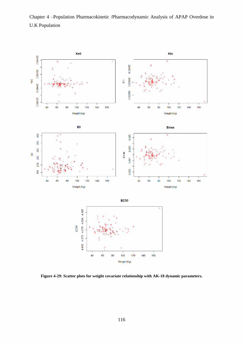
Chapter 4 –Population Pharmacokinetic /Pharmacodynamic Analysis of APAP Overdose in
U.K Population
116
Figure 4-29: Scatter plots for weight covariate relationship with AK-18 dynamic parameters.

Chapter 4 –Population Pharmacokinetic /Pharmacodynamic Analysis of APAP Overdose in
U.K Population
117
Figure 4-30: Boxplots of AK-18 pharmacodynamic model parameters categorized by gender

Chapter 4 –Population Pharmacokinetic /Pharmacodynamic Analysis of APAP Overdose in
U.K Population
118
Figure 4-31: Boxplots of AK-18 pharmacodynamic model parameters categorized by alcoholism Status.

Chapter 4 –Population Pharmacokinetic /Pharmacodynamic Analysis of APAP Overdose in
U.K Population
119
4.3.6. Necrosis K-18 PKPD Analysis
210 serum blood samples collected from 94 subjects were available for Pop-PKPD analysis for
the Necrosis K-18 (NK-18) biomarker with minimum of 2 samples at different time points per
patient. Parameter estimates of the Pop-PKPD model fit to the AK-18 biomarker data using the
ADVAN 13 subroutine are summarised in (Table 4-15). The population mean estimate for E0
(baseline of observed NK-18) was 198 U/L, which is within the normal range of human NK-
18activity (57-199 U/L). The maximum predicted response after APAP overdose (as given by
Emax) was an inhibition of 239% in the Kout dissipation parameter of the indirect effect PD
model. The estimated IIV for each structural model parameter, as well as the residual error
component of the model, was high and likely reflects the noisy and sparse nature of the data
where there was significant variability between patients in response to APAP induced liver
injury.
Table 4-15: Population Mean Estimates of Necrosis K-18 Pharmacodynamic Model Parameters.
Model Parameter Unit Final
Model
RES%a Bootstrapb
Median
Biasb Relative
Bias%b
95% CIc
Fixed Effects KE0 (h) 0.26 38 0.31 -0.05 -19 0.19-0.33
KIN (h) 0.54 48 0.46 0.08 14 0.4-0.68
E0 (U/l) 198 9 198 0 0 160-230
EMAX (%) 239 17.4 218 21 8 161-280
EC50 (mg/l) 2.13 37 2.5 -0.37 17 1.9-2.36
Random Effect
IIVd_KE0 (%CVe) 20 22 17 3 15 5-35
IIVd_KIN (%CVe) 62 50 62 0 0 10-114
IIVd_E0 (%CVe) 28 24 28 0 0 14-33
IIVd_EMAX (%CVe) 8 54 8 0 0 3-13
IIVd_EC50 (%CVe) 6 27 7 -1 -16 5-7
Residual Error (%CVe) 33 15 33 0 0 28-38
aRES; relative standard error = (standard error/final estimation)*100 bobtained from 320 bootstrap runs; bias = (final model estimate – bootstrap median); relative bias = 100 * ((final model estimate - bootstrap median) / final model estimate). cCI is Confidence Interval. dIIV is inter-individual variability of clearance. eCV is a coefficient variation.
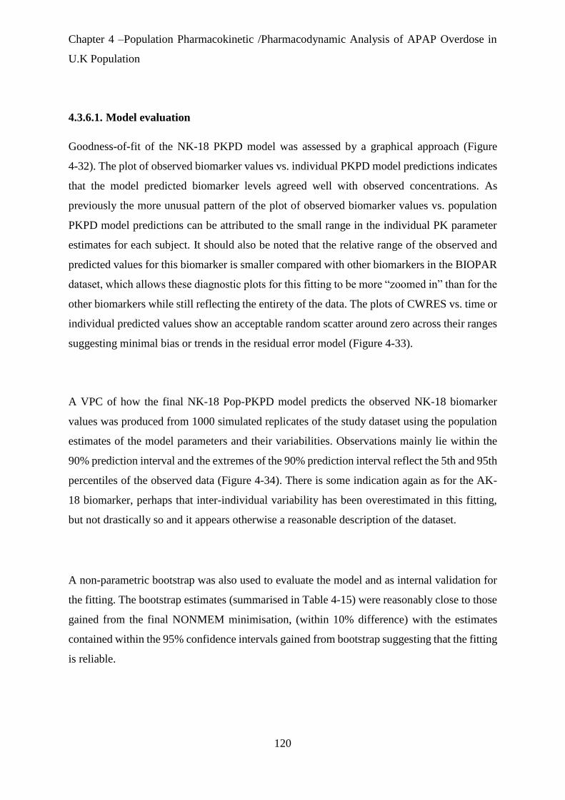
Chapter 4 –Population Pharmacokinetic /Pharmacodynamic Analysis of APAP Overdose in
U.K Population
120
4.3.6.1. Model evaluation
Goodness-of-fit of the NK-18 PKPD model was assessed by a graphical approach (Figure
4-32). The plot of observed biomarker values vs. individual PKPD model predictions indicates
that the model predicted biomarker levels agreed well with observed concentrations. As
previously the more unusual pattern of the plot of observed biomarker values vs. population
PKPD model predictions can be attributed to the small range in the individual PK parameter
estimates for each subject. It should also be noted that the relative range of the observed and
predicted values for this biomarker is smaller compared with other biomarkers in the BIOPAR
dataset, which allows these diagnostic plots for this fitting to be more “zoomed in” than for the
other biomarkers while still reflecting the entirety of the data. The plots of CWRES vs. time or
individual predicted values show an acceptable random scatter around zero across their ranges
suggesting minimal bias or trends in the residual error model (Figure 4-33).
A VPC of how the final NK-18 Pop-PKPD model predicts the observed NK-18 biomarker
values was produced from 1000 simulated replicates of the study dataset using the population
estimates of the model parameters and their variabilities. Observations mainly lie within the
90% prediction interval and the extremes of the 90% prediction interval reflect the 5th and 95th
percentiles of the observed data (Figure 4-34). There is some indication again as for the AK-
18 biomarker, perhaps that inter-individual variability has been overestimated in this fitting,
but not drastically so and it appears otherwise a reasonable description of the dataset.
A non-parametric bootstrap was also used to evaluate the model and as internal validation for
the fitting. The bootstrap estimates (summarised in Table 4-15) were reasonably close to those
gained from the final NONMEM minimisation, (within 10% difference) with the estimates
contained within the 95% confidence intervals gained from bootstrap suggesting that the fitting
is reliable.
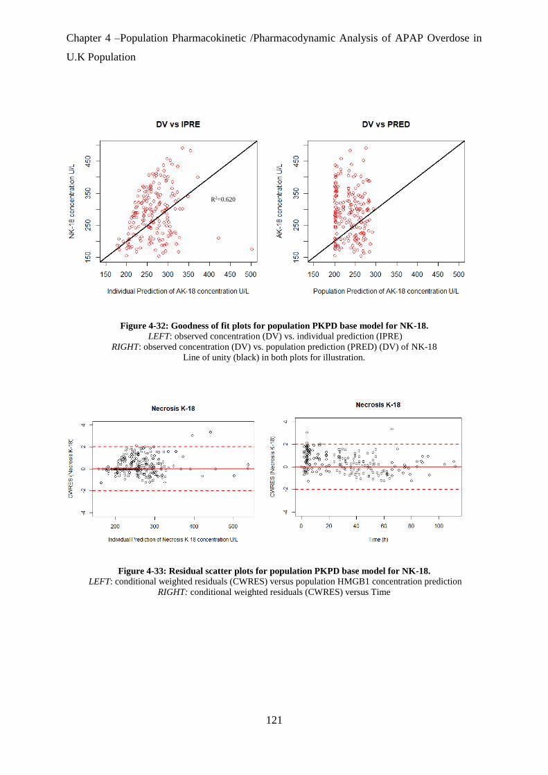
Chapter 4 –Population Pharmacokinetic /Pharmacodynamic Analysis of APAP Overdose in
U.K Population
121
Figure 4-32: Goodness of fit plots for population PKPD base model for NK-18.
LEFT: observed concentration (DV) vs. individual prediction (IPRE)
RIGHT: observed concentration (DV) vs. population prediction (PRED) (DV) of NK-18
Line of unity (black) in both plots for illustration.
Figure 4-33: Residual scatter plots for population PKPD base model for NK-18.
LEFT: conditional weighted residuals (CWRES) versus population HMGB1 concentration prediction
RIGHT: conditional weighted residuals (CWRES) versus Time
R2=0.620
.62
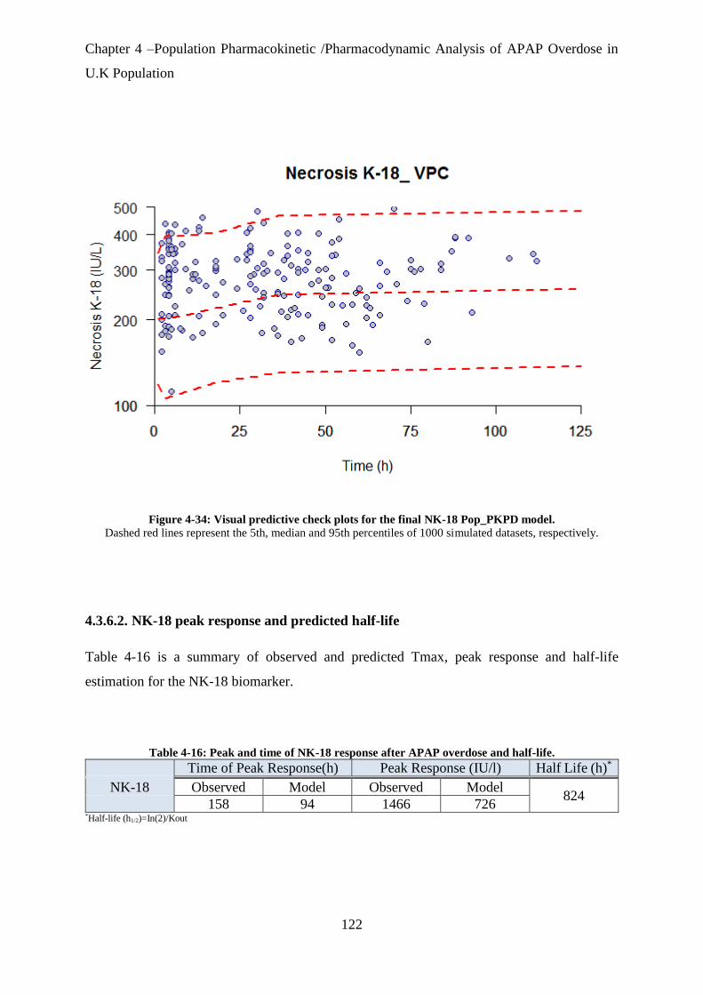
Chapter 4 –Population Pharmacokinetic /Pharmacodynamic Analysis of APAP Overdose in
U.K Population
122
Figure 4-34: Visual predictive check plots for the final NK-18 Pop_PKPD model.
Dashed red lines represent the 5th, median and 95th percentiles of 1000 simulated datasets, respectively.
4.3.6.2. NK-18 peak response and predicted half-life
Table 4-16 is a summary of observed and predicted Tmax, peak response and half-life
estimation for the NK-18 biomarker.
Table 4-16: Peak and time of NK-18 response after APAP overdose and half-life.
Time of Peak Response(h) Peak Response (IU/l) Half Life (h)*
NK-18 Observed Model Observed Model 824
158 94 1466 726 *Half-life (h1/2)=In(2)/Kout

Chapter 4 –Population Pharmacokinetic /Pharmacodynamic Analysis of APAP Overdose in
U.K Population
123
4.3.6.3. Covariate effects on NK-18 PD model.
Figure 4-35 and Figure 4-36 display scatter plots for continuous covariates of weight and age
vs individual subject estimates (posthoc and empirical Bayes estimates) of the NK-18 PD
model parameters. No major covariate effects for age or weight appear to be indicated for NK-
18 PD model parameters in these plots.
Figure 4-37 and Figure 4-38 contain boxplots of individual subject estimates of NK-18 PD
model parameters stratified according to categorical pairwise covariates of gender and
alcoholism status to indicate these potential group/categorical effects on the PD model
parameters. Table 4-17 summarises the statistical significance and the mean differences for the
pairwise categorical covariate effects on the NK-18 PD model parameters.
There are statistically significant differences between Male vs. Female and Alcoholic vs. Non-
Alcoholic for some PD model parameters. In these cases however, even though the difference
may show some statistical significance, the differences in the means of the two categorised
groups is always very small, i.e. a fractional difference with a small dynamic change according
to category. Broadly therefore it can be concluded that neither categorical covariate effect
(gender or alcoholism) on any of the NK-18 PD model parameters needs to be accounted for
and can be excluded from further analyses of this data.
Table 4-17: T. test statistical analysis for categorical covariate effects on NK-18 biomarker PD
parameters
Covariates Alcoholism Status Gender
Parameters Ke0 Kin E0 Emax EC50 Ke0 Kin E0 Emax EC50
Difference
in means -0.001 0.001 0.02 0.001 -0.0001 0.0002 0.001 0.02 0.001 0.00002
P value 0.001 0.228 0.48 0.22 0.008 0.23 0.1 0.51 0.15 0.688
Underline denotes p<0.05 and therefore significant
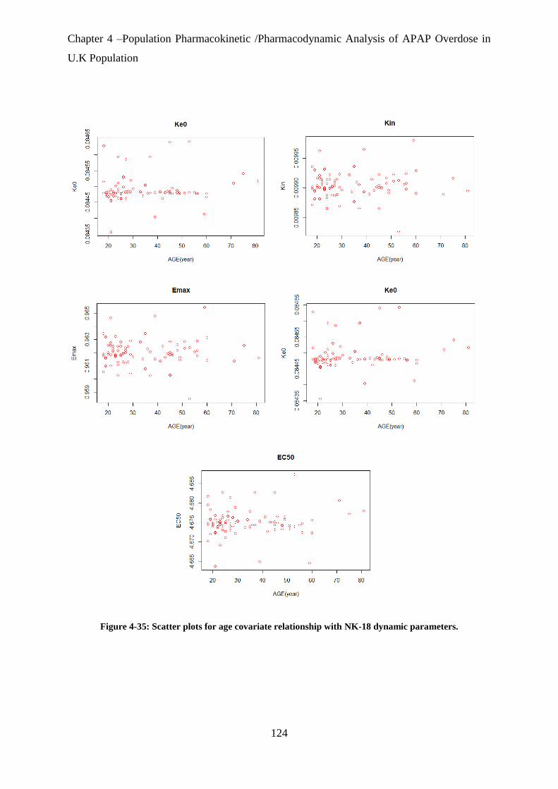
Chapter 4 –Population Pharmacokinetic /Pharmacodynamic Analysis of APAP Overdose in
U.K Population
124
Figure 4-35: Scatter plots for age covariate relationship with NK-18 dynamic parameters.

Chapter 4 –Population Pharmacokinetic /Pharmacodynamic Analysis of APAP Overdose in
U.K Population
125
Figure 4-36: Scatter plots for weight covariate relationship with NK-18 dynamic parameters.

Chapter 4 –Population Pharmacokinetic /Pharmacodynamic Analysis of APAP Overdose in
U.K Population
126
Figure 4-37: Boxplots of NK-18 pharmacodynamic model parameters categorized by gender
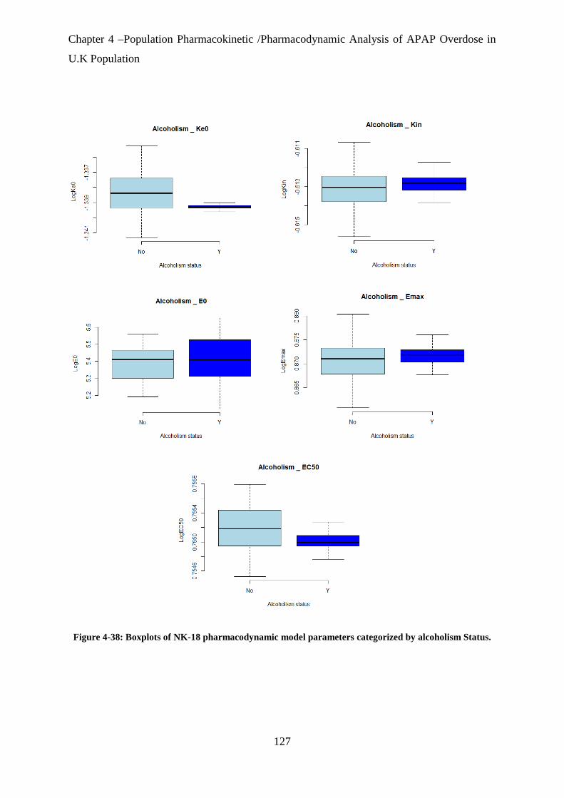
Chapter 4 –Population Pharmacokinetic /Pharmacodynamic Analysis of APAP Overdose in
U.K Population
127
Figure 4-38: Boxplots of NK-18 pharmacodynamic model parameters categorized by alcoholism Status.
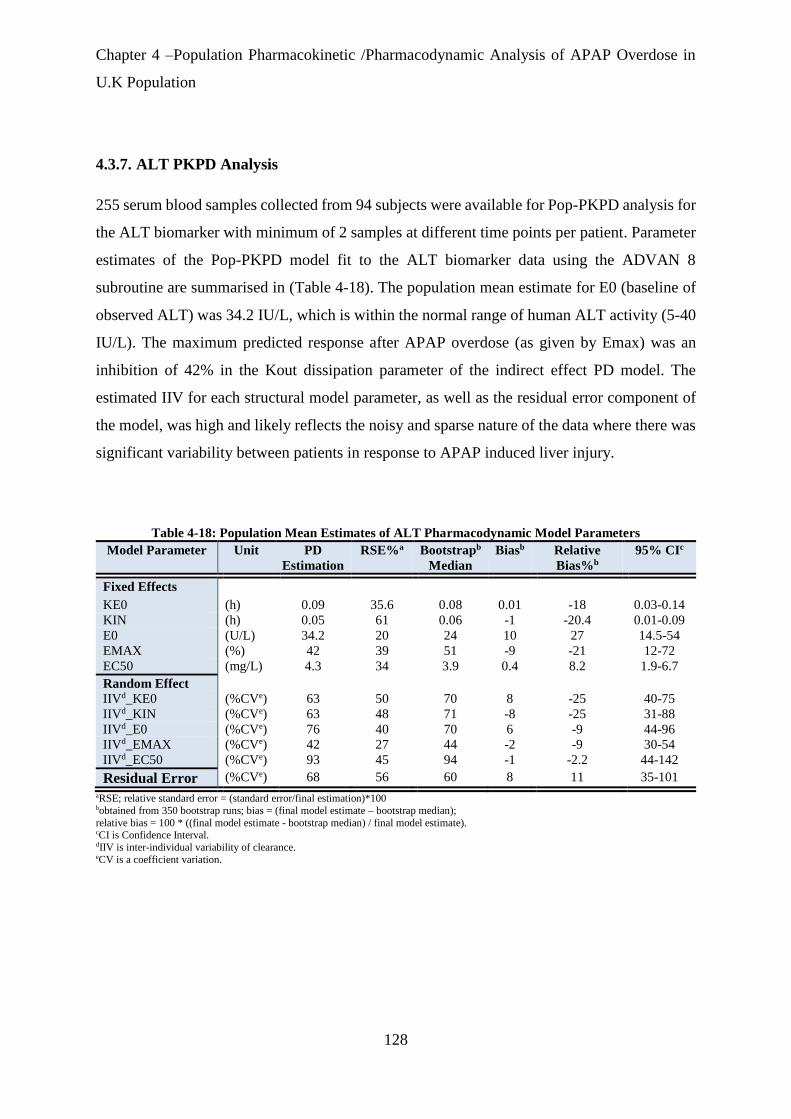
Chapter 4 –Population Pharmacokinetic /Pharmacodynamic Analysis of APAP Overdose in
U.K Population
128
4.3.7. ALT PKPD Analysis
255 serum blood samples collected from 94 subjects were available for Pop-PKPD analysis for
the ALT biomarker with minimum of 2 samples at different time points per patient. Parameter
estimates of the Pop-PKPD model fit to the ALT biomarker data using the ADVAN 8
subroutine are summarised in (Table 4-18). The population mean estimate for E0 (baseline of
observed ALT) was 34.2 IU/L, which is within the normal range of human ALT activity (5-40
IU/L). The maximum predicted response after APAP overdose (as given by Emax) was an
inhibition of 42% in the Kout dissipation parameter of the indirect effect PD model. The
estimated IIV for each structural model parameter, as well as the residual error component of
the model, was high and likely reflects the noisy and sparse nature of the data where there was
significant variability between patients in response to APAP induced liver injury.
Table 4-18: Population Mean Estimates of ALT Pharmacodynamic Model Parameters
Model Parameter Unit PD
Estimation
RSE%a Bootstrapb
Median
Biasb Relative
Bias%b
95% CIc
Fixed Effects KE0 (h) 0.09 35.6 0.08 0.01 -18 0.03-0.14
KIN (h) 0.05 61 0.06 -1 -20.4 0.01-0.09
E0 (U/L) 34.2 20 24 10 27 14.5-54
EMAX (%) 42 39 51 -9 -21 12-72
EC50 (mg/L) 4.3 34 3.9 0.4 8.2 1.9-6.7
Random Effect
IIVd_KE0 (%CVe) 63 50 70 8 -25 40-75
IIVd_KIN (%CVe) 63 48 71 -8 -25 31-88
IIVd_E0 (%CVe) 76 40 70 6 -9 44-96
IIVd_EMAX (%CVe) 42 27 44 -2 -9 30-54
IIVd_EC50 (%CVe) 93 45 94 -1 -2.2 44-142
Residual Error (%CVe) 68 56 60 8 11 35-101
aRSE; relative standard error = (standard error/final estimation)*100 bobtained from 350 bootstrap runs; bias = (final model estimate – bootstrap median);
relative bias = 100 * ((final model estimate - bootstrap median) / final model estimate). cCI is Confidence Interval. dIIV is inter-individual variability of clearance. eCV is a coefficient variation.

Chapter 4 –Population Pharmacokinetic /Pharmacodynamic Analysis of APAP Overdose in
U.K Population
129
4.3.7.1. Model evaluation
Goodness-of-fit of the ALT PKPD model was assessed by a graphical approach (Figure 4-39).
The plot of observed biomarker values vs. individual PKPD model predictions indicates that
the model predictions of biomarker levels should be accepted with caution, but do represent
the best that was achievable with the dataset. As for the other biomarkers in the dataset the plot
of observed biomarker values vs. population PKPD model predictions looks more unusual, but
could be attributable to the small range in the individual PK parameter estimates for each
subject. The plot of CWRES vs. individual predicted values is approximately randomly
scattered around zero across its range suggesting acceptable bias in the residual error model,
though there are “runs” of positive and negative residuals at several points across the range of
biomarker concentrations (both low and high levels). There may also be some indication of
systematic overprediction suggested by the CWRES vs. time plot (Figure 4-40). The ALT
model fitting included here however gave relatively acceptable other diagnostic plots was
therefore settled on as the best that could be achieved with the data at hand after numerous
attempts.
A VPC of how the final ALT Pop-PKPD model predicts the observed ALT biomarker values
was produced from 1000 simulated replicates of the study dataset using the population
estimates of the model parameters and their variabilities. Observations mainly lie within the
90% prediction interval and the extremes of the 90% prediction interval reflect the 5th and 95th
percentiles of the observed data (Figure 4-41). The central tendency of the VPC prediction
interval (median) appears to lie somewhat above the central tendency of the observed data,
reflecting again some degree of overprediction in the model fitting. There is also some
indication that inter-individual variability has been overestimated in this fitting, but as for
previous biomarkers not drastically and it appears otherwise a reasonable description of the
dataset variability is given with the parameter estimates in question.
A non-parametric bootstrap was also used to evaluate the model and as internal validation for
the fitting. The bootstrap estimates (summarised in Table 4-18) were reasonably close to those

Chapter 4 –Population Pharmacokinetic /Pharmacodynamic Analysis of APAP Overdose in
U.K Population
130
gained from the final NONMEM minimisation, (within 10% difference) with the estimates
contained within the 95% confidence intervals gained from bootstrap suggesting that the fitting
is reliable.
Figure 4-39: Goodness of fit plots for population PKPD base model for ALT.
LEFT: observed concentration (DV) vs. individual prediction (IPRE)
RIGHT: observed concentration (DV) vs. population prediction (PRED)
Line of unity (black) in both plots for illustration.
Figure 4-40: Residual scatter plots for population PKPD base model for ALT.
LEFT: conditional weighted residuals (CWRES) versus individual ALT concentration prediction
RIGHT: conditional weighted residuals (CWRES) versus time

Chapter 4 –Population Pharmacokinetic /Pharmacodynamic Analysis of APAP Overdose in
U.K Population
131
Figure 4-41: Visual predictive check plots for the final ALT Pop_PKPD model.
Dashed red lines represent the 5th, median and 95th percentiles of 1000 simulated datasets, respectively.
4.3.7.2. ALT peak response and predicted half-life
Table 4-19 is a summary of observed and predicted Tmax, peak response and half-life
estimation for the ALT biomarker:
Table 4-19: Peak of ALT response after APAP overdose and time to response and half life
Time of Peak Response(h) Peak Response (IU/l) Half Life (h)*
ALT Observed Model Observed Model 3015
172 119 4142 399 *Half-life (h1/2)=In(2)/Kout

Chapter 4 –Population Pharmacokinetic /Pharmacodynamic Analysis of APAP Overdose in
U.K Population
132
4.3.7.3. Covariate effects on ALT PD model.
Figure 4-42 and Figure 4-43 are scatter plots for continuous covariates of weight and age vs
individual subject estimates (i.e. posthoc, empirical Bayes estimates) of ALT PD model
parameters. No covariate effects for age or weight appear to be indicated for ALT PD model
parameters in these plots.
Figure 4-44 and Figure 4-45 contain boxplots of individual subject estimates of ALT PD model
parameters stratified according to categorical pairwise covariates of gender and alcoholism
status to indicate their potential group/categorical effects on the PD model parameters. Table
4-20 summarises the statistical significance and the mean differences for the pairwise
categorical covariate effects on the ALT PD model parameters.
There are statistically significant differences between Male vs. Female and Alcoholic vs. Non-
Alcoholic for some PD model parameters. In these cases however, even though the difference
may show some statistical significance, the differences in the means of the two categorised
groups is always very small, i.e. a fractional difference with a small dynamic change according
to category. Broadly therefore it can be concluded that neither categorical covariate effect
(gender or alcoholism) on any of the ALT PD model parameters needs to be accounted for and
can be excluded from further analyses of this data.
Table 4-20: T. test statistical analysis for categorical covariate effects on ALT biomarker PD parameters.
Covariates Alcoholism Status Gender
Parameters Ke0 Kin E0 Emax EC50 Ke0 Kin E0 Emax EC50
Difference
in means 0.00041 0.002 0.02 -0.004 -0.001 -0.0002 0.0001 -0.02 0.0001 -0.0001
P value 0.0012 0.0007 0.11 0.0013 0.00001 0.0006 0.9 0.11 0.68 0.86
Underline denotes p<0.05 and therefore significant

Chapter 4 –Population Pharmacokinetic /Pharmacodynamic Analysis of APAP Overdose in
U.K Population
133
Figure 4-42: Scatter plots for age covariate relationship with ALT dynamic parameters.

Chapter 4 –Population Pharmacokinetic /Pharmacodynamic Analysis of APAP Overdose in
U.K Population
134
Figure 4-43: Scatter plots for weight covariate relationship with NK-18 dynamic parameters.

Chapter 4 –Population Pharmacokinetic /Pharmacodynamic Analysis of APAP Overdose in
U.K Population
135
Figure 4-44: Boxplots of for ALT pharmacodynamic model parameters categorized by gender
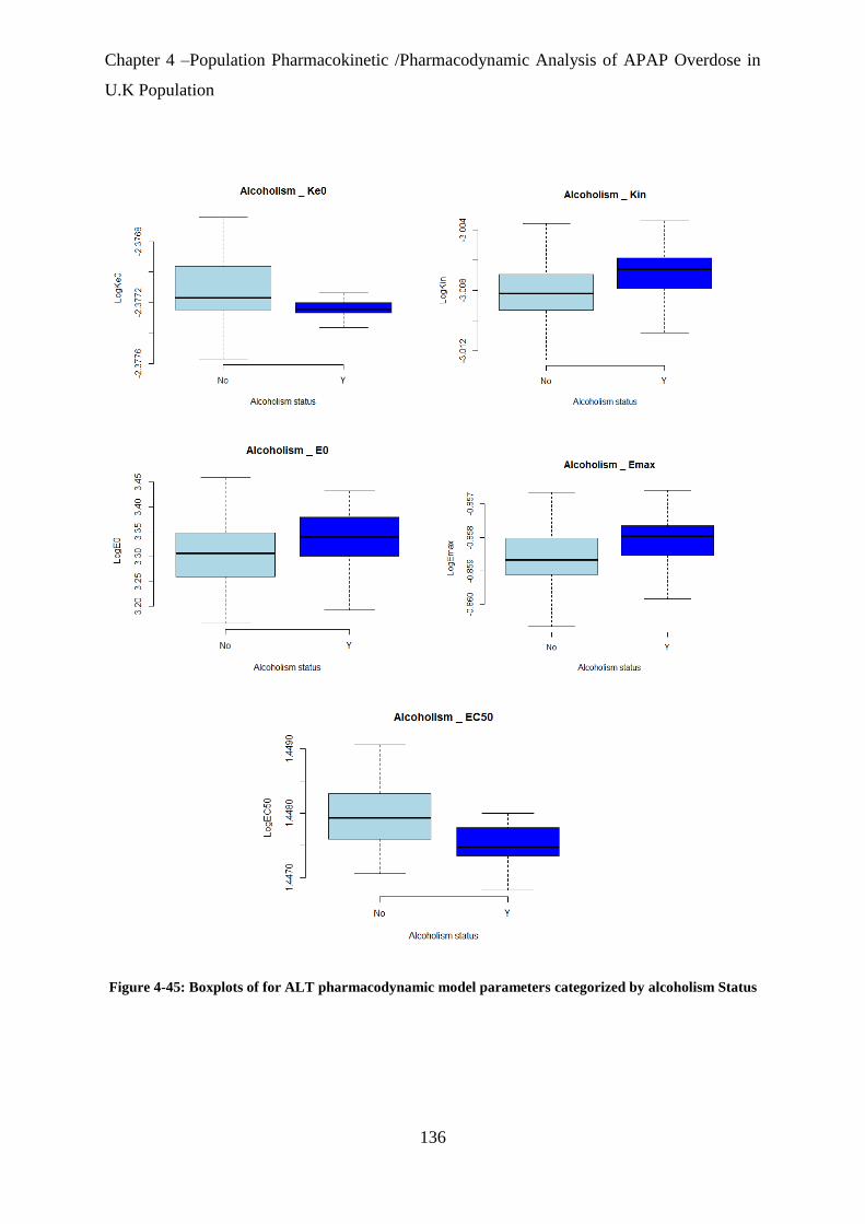
Chapter 4 –Population Pharmacokinetic /Pharmacodynamic Analysis of APAP Overdose in
U.K Population
136
Figure 4-45: Boxplots of for ALT pharmacodynamic model parameters categorized by alcoholism Status
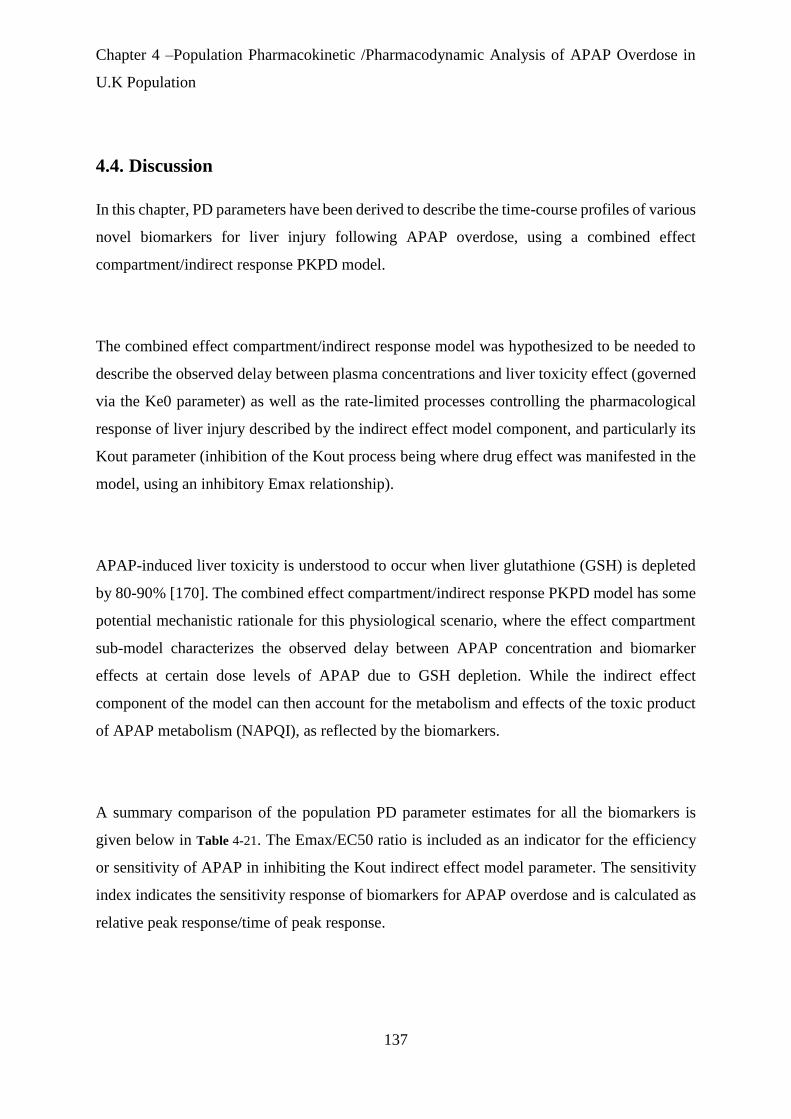
Chapter 4 –Population Pharmacokinetic /Pharmacodynamic Analysis of APAP Overdose in
U.K Population
137
4.4. Discussion
In this chapter, PD parameters have been derived to describe the time-course profiles of various
novel biomarkers for liver injury following APAP overdose, using a combined effect
compartment/indirect response PKPD model.
The combined effect compartment/indirect response model was hypothesized to be needed to
describe the observed delay between plasma concentrations and liver toxicity effect (governed
via the Ke0 parameter) as well as the rate-limited processes controlling the pharmacological
response of liver injury described by the indirect effect model component, and particularly its
Kout parameter (inhibition of the Kout process being where drug effect was manifested in the
model, using an inhibitory Emax relationship).
APAP-induced liver toxicity is understood to occur when liver glutathione (GSH) is depleted
by 80-90% [170]. The combined effect compartment/indirect response PKPD model has some
potential mechanistic rationale for this physiological scenario, where the effect compartment
sub-model characterizes the observed delay between APAP concentration and biomarker
effects at certain dose levels of APAP due to GSH depletion. While the indirect effect
component of the model can then account for the metabolism and effects of the toxic product
of APAP metabolism (NAPQI), as reflected by the biomarkers.
A summary comparison of the population PD parameter estimates for all the biomarkers is
given below in Table 4-21. The Emax/EC50 ratio is included as an indicator for the efficiency
or sensitivity of APAP in inhibiting the Kout indirect effect model parameter. The sensitivity
index indicates the sensitivity response of biomarkers for APAP overdose and is calculated as
relative peak response/time of peak response.

Chapter 4 –Population Pharmacokinetic /Pharmacodynamic Analysis of APAP Overdose in
U.K Population
138
Table 4-21: Summary of the comparison PD biomarkers.
Emax
%
EC50
mg/l
Emax
/EC50
E0
h-1
Half
-
life*
Ke0
h-1
Model
Time of
Peak
Responsea
(h)
Model
Peak
Response
Model
relative
peak
responseb
Sensitivity
Indexc
HMGB1
ng/ml 102 0.32 3.19 1.14 940 0.5 128 35 2970 23.2
Mir-122 Let-
7dnormalized 36 1.81 0.20 0.57 121 0.01 70 25 4285 61.2
GLDH U/L
105 0.53 1.98 15.1 560 0.06 177 507 3257 18.4
AK-18 U/L
96 4.5 0.21 197 283
10 0.08 194 461 134 0.69
NK-18 U/L
239 2.3 1.04 198 824 0.26 94 726 266 2.8
ALT U/L
42 4.3 0.10 34.2 301
5 0.09 119 399 1066 8.9
aHalf-life=ln(2)/kout bModel relative peak response = (model peak response-E0)/E0 *100 cSensitivity index = relative peak response/time of peak response
The inhibitory Emax effect of APAP on the Kout parameter was highest for the NK-18
biomarker and was estimated as greater than 100% for this biomarker, with model fitting
attempts where this Emax was bounded to be less than or equal to 100% not giving a good
description of the NK-18 dataset. Considering Equation 4-5, an Emax >100% would change
the sign of the Kout driven dissipation process, i.e. “flipping” the process when the drug effect
was of sufficient magnitude, giving in effect two production processes to increase the observed
indirect effect response in a form of positive feedback (Figure 4-46). However, NK-18 is a less
sensitive index for APAP overdose response compare with other biomarkers.
miR-122 has the highest sensitivity index compared with other biomarkers in response of
APAP overdose. The inhibitory Emax effect of APAP on Kout is lowest for the miR-122
biomarker, which also has the shortest half-life and the shortest Tmax to reach its peak effect.
Further, the peak effect appears quickest and with highest magnitude relative to baseline
compared with other biomarkers. These results agree with the findings of other studies in which
miR-122 has been considered more sensitive than ALT as a biomarker of liver injury (i.e. it is
released faster than ALT after APAP overdose) [71].

Chapter 4 –Population Pharmacokinetic /Pharmacodynamic Analysis of APAP Overdose in
U.K Population
139
Figure 4-46:Sequential effect compartment/indirect effect model – illustration of potential positive
feedback if Emax >100 for Kout dissipation process of indirect effect
Based on the ratio of Emax to EC50, HMGB1 response may potentially be the most sensitive
to APAP levels. This is combined with a comparatively small Ke0, however only simulations
can reveal whether these parameters will translate to HMGB1 having the earliest detection
point above its normal clinical range as an indicator of potential liver injury.
Previously, K-18 biomarkers of both necrosis and apoptosis types were also identified as more
sensitive than ALT in predicting liver injury [171]. The AK-18 biomarker has the longest mean
half-life compared with the others in this study (as calculated from the Kout parameter). This
long biomarker half-life is potentially consistent with characteristics of apoptosis (i.e.
programmed cell death) where AK-18 is activated and goes on to act as both an initiator and

Chapter 4 –Population Pharmacokinetic /Pharmacodynamic Analysis of APAP Overdose in
U.K Population
140
effector of cell death after liver injury. The long half-life may also be indicative of longer-term
liver injury, which may be recoverable or permanent, and which may not be reflected in the
behaviour of other biomarkers.
ALT has long been considered as the gold standard for clinical evaluation of liver injury. The
PKPD models of ALT results need to be interpreted with caution, due to the wide variability
between patients. The relatively poor fitting of the ALT data in this study compared with the
other biomarkers further justifies the use of novel biomarkers to predict subsequent liver injury.
Further work in the next chapter will use the parameter estimates calculated in this chapter to
investigate various scenarios and assess the relative abilities of the various biomarkers to
predict liver injury outcome.

Chapter 5 – Simulation and Exploration of Novel Biomarkers in APAP induced Liver Injury
Introduction
141
Chapter-5.
Simulation and Exploration of
Novel Biomarkers in APAP
induced Liver Injury
Introduction

Chapter 5 – Simulation and Exploration of Novel Biomarkers in APAP induced Liver Injury
Introduction
142
Chapter 5. Simulation and Exploration of Novel Biomarkers in
APAP induced Liver Injury Introduction
5.1. Introduction
The novel biomarkers HMGB1, miR-122, GLDH, NK-18 and AK-18 have been indicated as
predictive biomarkers for DILI in animal models [172]. Recently, the potential prediction of
DILI using these biomarkers has become of wider interest meaning significant investment and
progress has been made in this area [173]. Even though a recent study has shown the sensitivity
and specificity of these biomarkers in human [61], using the biomarkers to predict DILI in
humans has still remained difficult because of inter-individual variability (IIV). In the previous
chapters 3 and 4, a PKPD dataset of these novel biomarkers following an APAP overdose
(where liver injury was recorded in a proportion of the patients) has been modelled with a
population approach, with specific consideration of the IIV (i.e. to attempt to quantify and
explain the IIV in the data, as well as its other trends and relationships) to facilitate its use in
predictions.
Using the Pop-PKPD model parameters estimates from the PKPD models fitted thus far, a
simulation approach will be used in this chapter to investigate the wider implications of the
data and to assess the early prediction ability of these novel biomarkers after APAP overdose.
The overall aim will be to define particular clinical scenarios for which novel biomarkers after
APAP overdose could serve as combined tests or replace existing diagnostic approaches (e.g.
ALT) that predict liver injury with greater sensitivity and/or specificity [156].
5.1.1. Receiver Operating Characteristic (ROC) Analysis
The growing need for rigorous evaluation of novel biomarkers in medical practice has
encouraged the development and characterization of statistical methods for assessing
diagnostic accuracy of biomarkers and the receiver operating characteristic (ROC) is
considered a robust algorithm for this assessment [174]. It is a widely used method and well-

Chapter 5 – Simulation and Exploration of Novel Biomarkers in APAP induced Liver Injury
Introduction
143
known in engineering applications to evaluate the performance of binary classification models.
It originated in the early 1950s and the first application was in radar signals to detect enemy
airplanes during World War II, and was also used in psychological experiments to determine
the relationship between properties of physical stimuli and the attributes of psychological
experience.
During the last four decades, ROC analysis has been applied extensively for evaluating the
accuracy of medical diagnostic systems.[174]. The biomarkers falls into 5 major categorise,
which are: diagnostic, prognostic, predictive, monitoring and exposure. ROC can be especially
useful to novel biomarkers for DILI prediction as it can visualise the unbiased trade-off
between sensitivity (i.e. the ability of the biomarker to identify the toxicity when it occurs) and
specificity (i.e. the ability of biomarker to identify the individual is not have toxicity).
ROC analysis is based on the concept of a “separator” variable where the frequencies of a
positive or negative diagnosis (or categorisation into one group or another, according to the
values of the test in question) will change with alteration in the cut-off or criterion. For
example, a particular cut-off value will be derived for a biomarker level, at a particular
timepoint to determine a prognosis of DILI or not. This can be compared vs. the true eventual
outcome to see if the biomarker at that cut-off value has correctly diagnosed the patient for
DILI or not. The result will therefore be one of either: a true/false positive, or true/false negative
(Table 5-1).
The hypothesis of an ROC analysis plot therefore is to display a signal to noise ratio, identifying
a true positive fraction (TPF) that is a correct signal from diagnostic test (known as
“sensitivity”) and a false positive fraction (FPF) known as “specificity” at various threshold
cut-off values of a diagnostic test. Applied specifically to the DILI example, the fraction of
patients with actual DILI (as measured by peak ALT) correctly also diagnosed as such (using
a threshold) by their biomarker level represent a the true positive, while patients without actual
DILI whose biomarker level using that threshold says that they do have DILI represent a false
positive [176].

Chapter 5 – Simulation and Exploration of Novel Biomarkers in APAP induced Liver Injury
Introduction
144
On an ROC plot showing TPF vs. FPF (e.g. Figure 5-1(right)) the red diagonal line is
corresponds to a test that predicts outcome as positive or negative no better than chance. The
greater the discriminatory capacity of a diagnostic test the more its ROC curve will be located
to the upper left-hand corner of “ROC space” in this plot, showing the best possible sensitivity
for the lowest loss in specificity. If two points from the curve were to be examined in detail, a
point further down to the left represents low sensitivity and higher specificity while a point on
the curve as it moves up and to the right shows high sensitivity and low specificity. The ROC
graphical curve is particularly useful to compare between two or more diagnostic tests which
may show different gain/loss in sensitivity vs. specificity (Figure 5-1(left)).
There are many advantages for ROC curve analysis compared with other methods for assessing
diagnostic accuracy [177]. It visually represents diagnostic accuracy by plotting sensitivity and
specificity at multiple threshold points and therefore can also provide a direct and visual
comparison of two or more tests on a single set of axes. A key property of ROC analysis also
is that the accuracy indices derived from the method, are not changed by fluctuations caused
by the use of illogically chosen decision criteria or cut-offs [178].
Table 5-1: Classification of ROC table
Test score Has DILI Does not have DILI
Positive True Positive Fraction
(TPF)
False Positive Fraction
(FPF) PPV
TPF/(TPF+FPF)
Negative False Negative Fraction
(FNF)
True Negative Fraction
(TNF) NPV
TNF/(TNF+FNF)
Sensitivity
TPF/(TPF+FNF) Specificity
TNF/(TNF+FPF)
PPV is positive predictive value.
NPV is a negative predictive value.
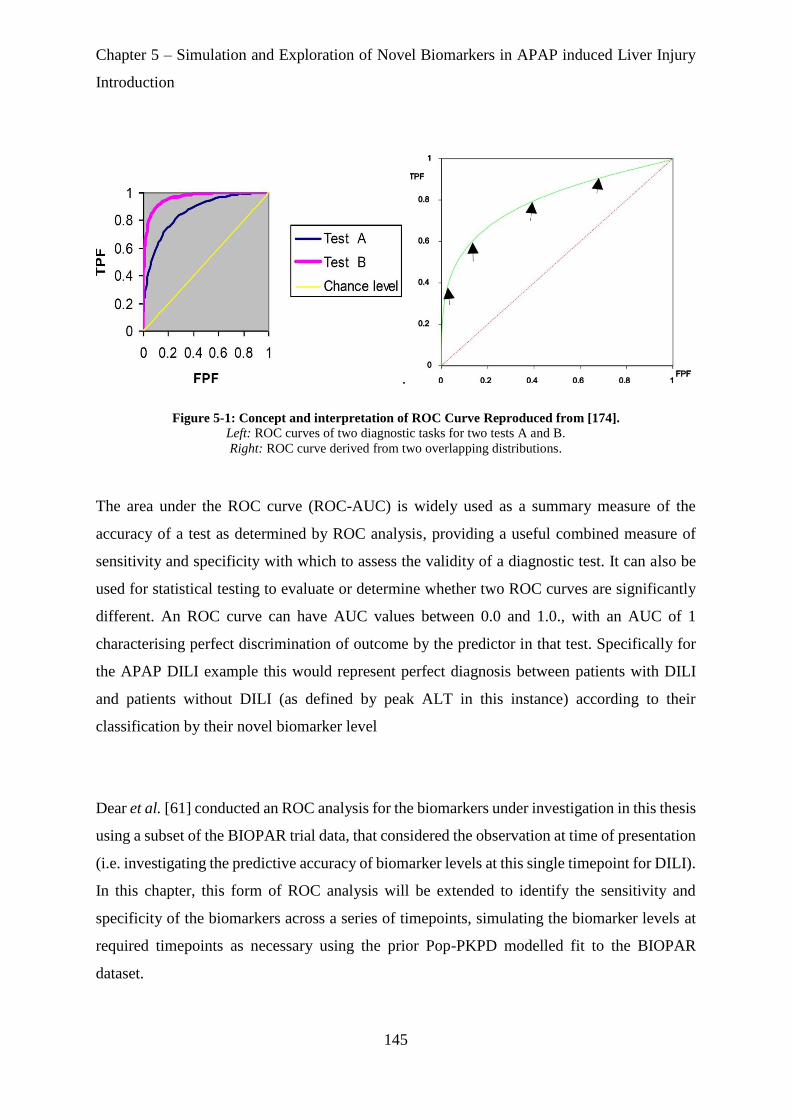
Chapter 5 – Simulation and Exploration of Novel Biomarkers in APAP induced Liver Injury
Introduction
145
.
Figure 5-1: Concept and interpretation of ROC Curve Reproduced from [174].
Left: ROC curves of two diagnostic tasks for two tests A and B.
Right: ROC curve derived from two overlapping distributions.
The area under the ROC curve (ROC-AUC) is widely used as a summary measure of the
accuracy of a test as determined by ROC analysis, providing a useful combined measure of
sensitivity and specificity with which to assess the validity of a diagnostic test. It can also be
used for statistical testing to evaluate or determine whether two ROC curves are significantly
different. An ROC curve can have AUC values between 0.0 and 1.0., with an AUC of 1
characterising perfect discrimination of outcome by the predictor in that test. Specifically for
the APAP DILI example this would represent perfect diagnosis between patients with DILI
and patients without DILI (as defined by peak ALT in this instance) according to their
classification by their novel biomarker level
Dear et al. [61] conducted an ROC analysis for the biomarkers under investigation in this thesis
using a subset of the BIOPAR trial data, that considered the observation at time of presentation
(i.e. investigating the predictive accuracy of biomarker levels at this single timepoint for DILI).
In this chapter, this form of ROC analysis will be extended to identify the sensitivity and
specificity of the biomarkers across a series of timepoints, simulating the biomarker levels at
required timepoints as necessary using the prior Pop-PKPD modelled fit to the BIOPAR
dataset.
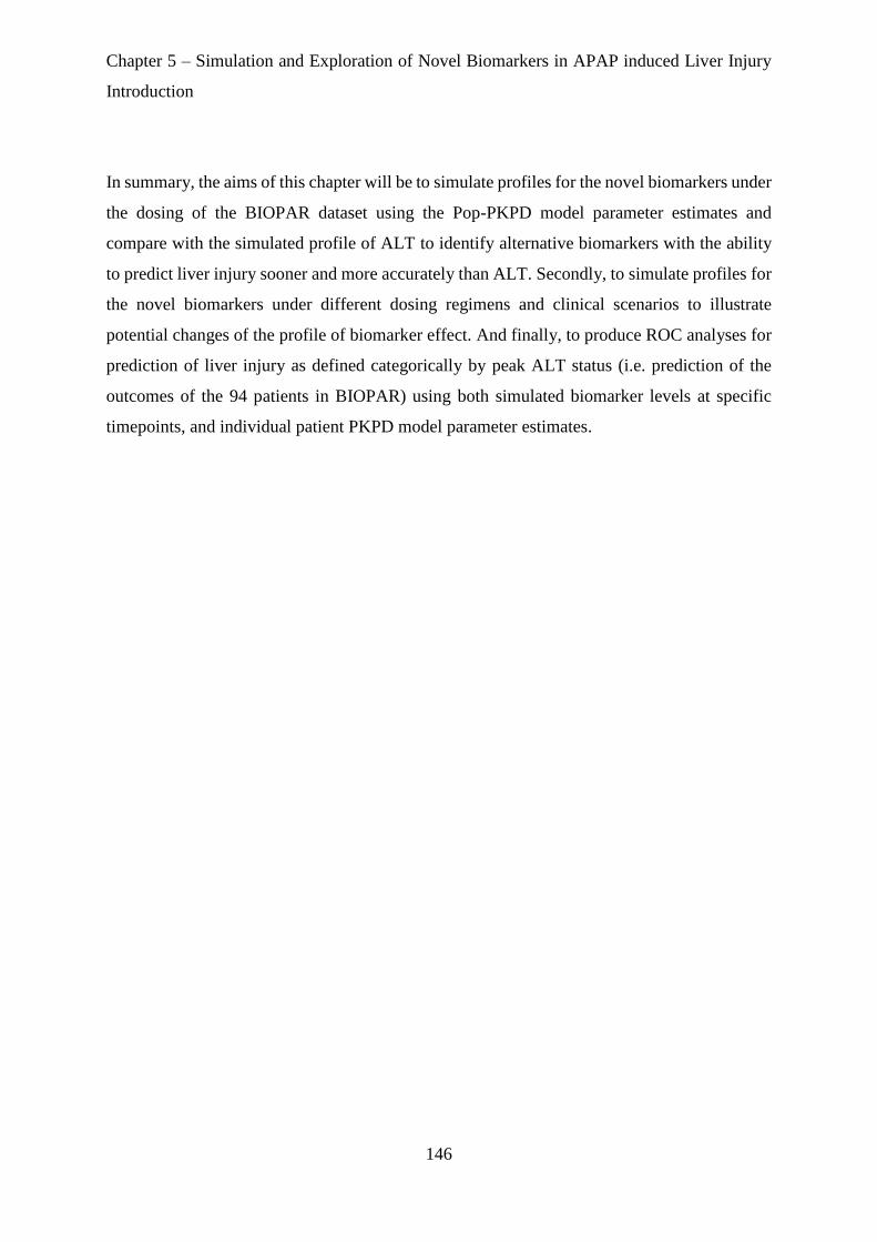
Chapter 5 – Simulation and Exploration of Novel Biomarkers in APAP induced Liver Injury
Introduction
146
In summary, the aims of this chapter will be to simulate profiles for the novel biomarkers under
the dosing of the BIOPAR dataset using the Pop-PKPD model parameter estimates and
compare with the simulated profile of ALT to identify alternative biomarkers with the ability
to predict liver injury sooner and more accurately than ALT. Secondly, to simulate profiles for
the novel biomarkers under different dosing regimens and clinical scenarios to illustrate
potential changes of the profile of biomarker effect. And finally, to produce ROC analyses for
prediction of liver injury as defined categorically by peak ALT status (i.e. prediction of the
outcomes of the 94 patients in BIOPAR) using both simulated biomarker levels at specific
timepoints, and individual patient PKPD model parameter estimates.

Chapter 5 – Simulation and Exploration of Novel Biomarkers in APAP induced Liver Injury
Introduction
147
5.2. Methods
Prediction of the phases within the network of biomarkers in response to liver injury resulting
from APAP overdose was achieved using time course effect simulation for each biomarker. An
ROC analysis was used to assess the sensitivity and specificity of each biomarker at various
timepoints to predict the optimal time point for DILI prediction. Data from patients recruited
in the BIOPAR clinical trial and the previous model fittings described in chapters 3 and 4 were
used in these analyses. Simulations were performed using both R 3.4.4 and NONMEM, and
the pROC package [175]was used for ROC analysis.
5.2.1. Simulation of Typical Patient and Population Biomarker Timecourse Effect
Profiles
The Pop-PKPD parameter estimates obtained from the final Pop-PKPD biomarker models (see
Chapter 4) were used to simulate rich time-courses of APAP concentrations and biomarkers
over 72 hours to give precise descriptions of the time courses of effect. These simulation
profiles can give an indication of the potential value of the biomarkers in early detection of
liver injury by comparison with the ALT profile (i.e. the baseline for liver injury) and
examining which biomarkers show the earliest and/or largest relative deviation from normal
range following APAP overdose. Simulations were carried out in R using the mean dose in the
BIOPAR trial (33g) and also included “typical patient” profiles derived from the fixed
effect/population mean model parameter values and also 1000 “trial/population simulation”
profiles generated using the random effects parameters for interindividual variability to show
the modelled variability in the biomarker levels across the population. (This trial/population
simulation will be illustrated on plots as a shaded prediction interval area).
5.2.2. Simulation of Different Clinical Scenarios
Simulation of profiles for all novel biomarkers under different dosing regimens, dose levels
and clinical scenarios (e.g. dosing patterns with multiple staggered doses and/or different
dosing intervals) were also conducted to illustrate potential changes of the profile of biomarker
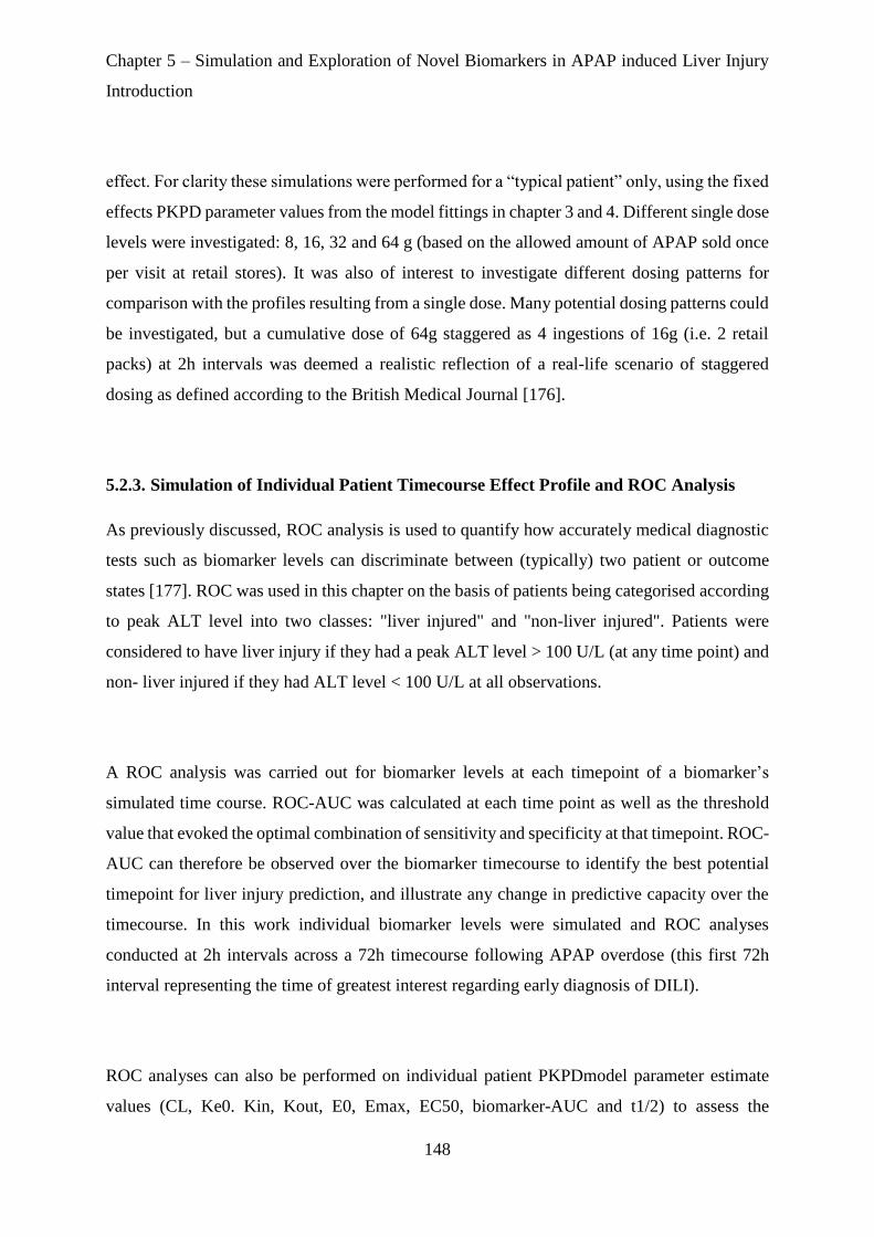
Chapter 5 – Simulation and Exploration of Novel Biomarkers in APAP induced Liver Injury
Introduction
148
effect. For clarity these simulations were performed for a “typical patient” only, using the fixed
effects PKPD parameter values from the model fittings in chapter 3 and 4. Different single dose
levels were investigated: 8, 16, 32 and 64 g (based on the allowed amount of APAP sold once
per visit at retail stores). It was also of interest to investigate different dosing patterns for
comparison with the profiles resulting from a single dose. Many potential dosing patterns could
be investigated, but a cumulative dose of 64g staggered as 4 ingestions of 16g (i.e. 2 retail
packs) at 2h intervals was deemed a realistic reflection of a real-life scenario of staggered
dosing as defined according to the British Medical Journal [176].
5.2.3. Simulation of Individual Patient Timecourse Effect Profile and ROC Analysis
As previously discussed, ROC analysis is used to quantify how accurately medical diagnostic
tests such as biomarker levels can discriminate between (typically) two patient or outcome
states [177]. ROC was used in this chapter on the basis of patients being categorised according
to peak ALT level into two classes: "liver injured" and "non-liver injured". Patients were
considered to have liver injury if they had a peak ALT level > 100 U/L (at any time point) and
non- liver injured if they had ALT level < 100 U/L at all observations.
A ROC analysis was carried out for biomarker levels at each timepoint of a biomarker’s
simulated time course. ROC-AUC was calculated at each time point as well as the threshold
value that evoked the optimal combination of sensitivity and specificity at that timepoint. ROC-
AUC can therefore be observed over the biomarker timecourse to identify the best potential
timepoint for liver injury prediction, and illustrate any change in predictive capacity over the
timecourse. In this work individual biomarker levels were simulated and ROC analyses
conducted at 2h intervals across a 72h timecourse following APAP overdose (this first 72h
interval representing the time of greatest interest regarding early diagnosis of DILI).
ROC analyses can also be performed on individual patient PKPDmodel parameter estimate
values (CL, Ke0. Kin, Kout, E0, Emax, EC50, biomarker-AUC and t1/2) to assess the

Chapter 5 – Simulation and Exploration of Novel Biomarkers in APAP induced Liver Injury
Introduction
149
predictivity of these parameters for DILI, although the clinical applicability of these parameters
as a practical diagnostic tool is limited because in most circumstance an entire dataset would
need to be analysed in order for them to be estimated.

Chapter 5 – Simulation and Exploration of Novel Biomarkers in APAP induced Liver Injury
Introduction
150
5.3. Results
5.3.1. Simulation Results for Typical Patient and Population Biomarker Timecourse
Effect Profiles.
The simulations of timecourses for novel biomarkers of DILI generally showed flat profile
shapes over 72h that did not deviate beyond the normal range of levels for the biomarkers, as
shown in Figure 5-3, Figure 5-5, Figure 5-7 and Figure 5-9, with the normal ranges shown in
Table 5-2 below. This is consistent with the dynamic range and time course of observations in
the raw biomarker data used for PKPD modelling shown in chapter 4.
Table 5-2: Normal range for novel biomarkers
Biomarkers 2.5th quantile
50th quantile
97.5th quantile
miR-122
(let-7d normalised) 0.17 0.95 6.40
HMGB1 (ng/ml) 0.22 1.24 2.34
FL K18 (U/l) 114 248 475
CC K18 (U/l) 57 132 272
GLDH (U/l) 0.46 1.40 27
The simulation for NK-18 however shows an increase for this biomarker beyond its normal
range of 57-197 U/L to >200 U/L by 4h and continuing to increase over a 72h periodFigure
5-11. The ALT profile over 72h is similarly flat and within its normal range as for the other
biomarkers.
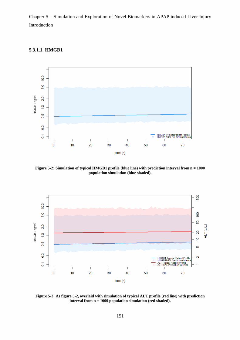
Chapter 5 – Simulation and Exploration of Novel Biomarkers in APAP induced Liver Injury
Introduction
151
5.3.1.1. HMGB1
Figure 5-2: Simulation of typical HMGB1 profile (blue line) with prediction interval from n = 1000
population simulation (blue shaded).
Figure 5-3: As figure 5-2, overlaid with simulation of typical ALT profile (red line) with prediction
interval from n = 1000 population simulation (red shaded).
HM
GB
1 n
g/m
l H
MG
B1
ng/m
l
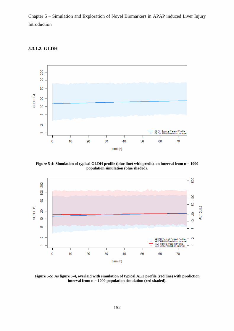
Chapter 5 – Simulation and Exploration of Novel Biomarkers in APAP induced Liver Injury
Introduction
152
5.3.1.2. GLDH
Figure 5-4: Simulation of typical GLDH profile (blue line) with prediction interval from n = 1000
population simulation (blue shaded).
Figure 5-5: As figure 5-4, overlaid with simulation of typical ALT profile (red line) with prediction
interval from n = 1000 population simulation (red shaded).
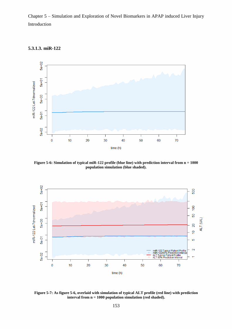
Chapter 5 – Simulation and Exploration of Novel Biomarkers in APAP induced Liver Injury
Introduction
153
5.3.1.3. miR-122
Figure 5-6: Simulation of typical miR-122 profile (blue line) with prediction interval from n = 1000
population simulation (blue shaded).
Figure 5-7: As figure 5-6, overlaid with simulation of typical ALT profile (red line) with prediction
interval from n = 1000 population simulation (red shaded).

Chapter 5 – Simulation and Exploration of Novel Biomarkers in APAP induced Liver Injury
Introduction
154
5.3.1.4. AK-18
Figure 5-8: Simulation of typical AK-18 profile (blue line) with prediction interval from n = 1000
population simulation (blue shaded).
Figure 5-9: As figure 5-8, overlaid with simulation of typical ALT profile (red line) with prediction
interval from n = 1000 population simulation (red shaded).
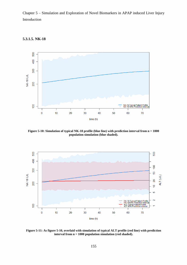
Chapter 5 – Simulation and Exploration of Novel Biomarkers in APAP induced Liver Injury
Introduction
155
5.3.1.5. NK-18
Figure 5-10: Simulation of typical NK-18 profile (blue line) with prediction interval from n = 1000
population simulation (blue shaded).
Figure 5-11: As figure 5-10, overlaid with simulation of typical ALT profile (red line) with prediction
interval from n = 1000 population simulation (red shaded).

Chapter 5 – Simulation and Exploration of Novel Biomarkers in APAP induced Liver Injury
Introduction
156
5.3.2. Simulation Results for Different Doses
Simulation of biomarker profiles over a time course of 72 hours following different doses of
APAP (8 g – 64 g) for a typical patient indicated that the release and accumulation of NK-18
biomarker shows a dose dependent increase with higher doses of APAP (Figure 5-16). The
profiles of other biomarkers appear dose independent and remained approximately constant
over the 72h time course and within their normal ranges (Figure 5-12, Figure 5-13, Figure 5-14
and Figure 5-15).
5.3.2.1. HMGB1
Figure 5-12: Effect Time-course simulations of HMGB1 at different doses of APAP.
Comparison of the time-course effect profile of HMGB1 (blue line) and ALT (red line) for a typical patient at
different doses.
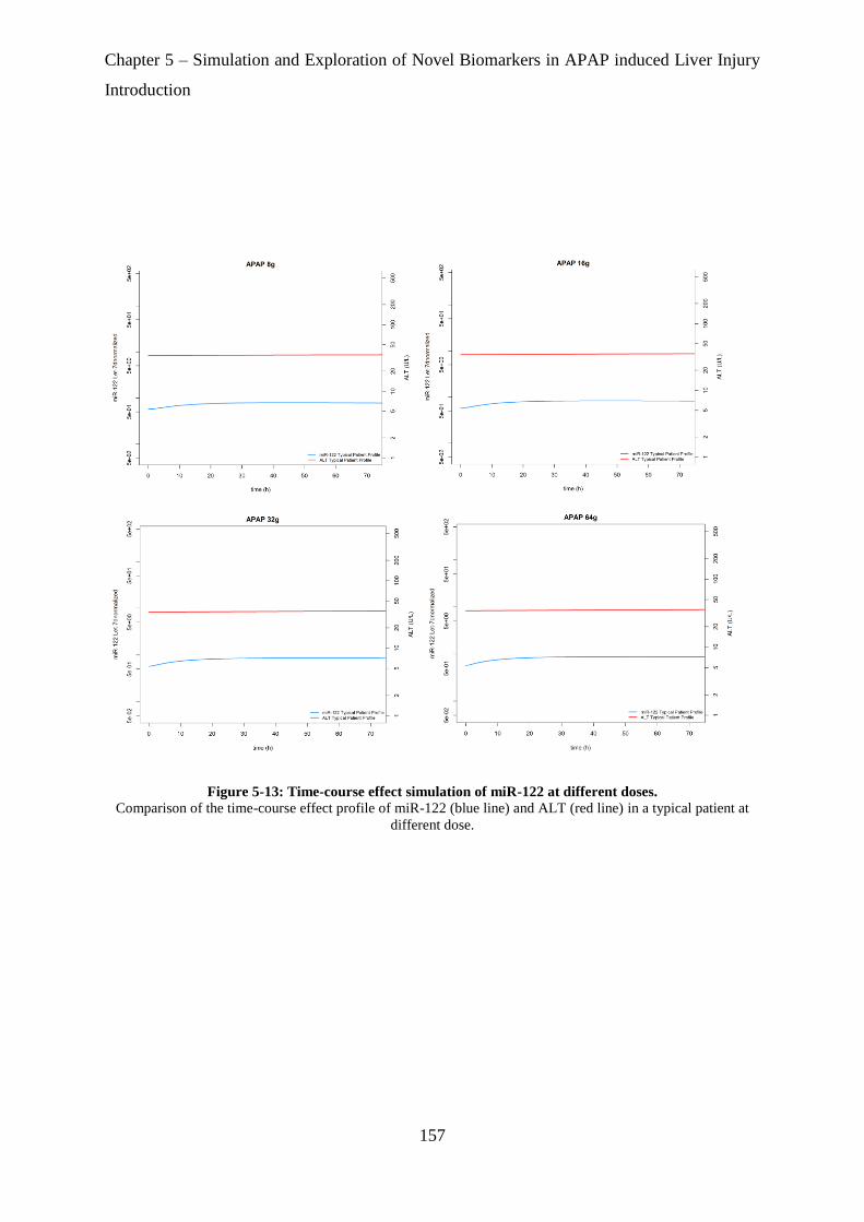
Chapter 5 – Simulation and Exploration of Novel Biomarkers in APAP induced Liver Injury
Introduction
157
Figure 5-13: Time-course effect simulation of miR-122 at different doses.
Comparison of the time-course effect profile of miR-122 (blue line) and ALT (red line) in a typical patient at
different dose.

Chapter 5 – Simulation and Exploration of Novel Biomarkers in APAP induced Liver Injury
Introduction
158
5.3.2.2. GLDH
Figure 5-14: Time-course effect simulation of GLDH at different doses.
Comparison of the time-course effect profile of GLDH (blue line) and ALT (red line) in a typical patient at
different dose.

Chapter 5 – Simulation and Exploration of Novel Biomarkers in APAP induced Liver Injury
Introduction
159
5.3.2.3. AK-18
Figure 5-15: Time-course effect simulation of AK-18 at different doses.
Comparison of the time-course effect profile of AK-18 (blue line) and ALT (red line) in a typical patient at
different dose.

Chapter 5 – Simulation and Exploration of Novel Biomarkers in APAP induced Liver Injury
Introduction
160
5.3.2.4. NK-18
Figure 5-16: Time-course effect simulation of NK-18 at different doses.
Comparison of the time-course effect profile of NK-18 (blue line) and ALT (red line) in a typical patient at
different dose.

Chapter 5 – Simulation and Exploration of Novel Biomarkers in APAP induced Liver Injury
Introduction
161
5.3.3. Simulation Results for Staggered Doses
Simulation results for a typical patient obtained from a staggered dosing regimen (Figure 5-17,
Figure 5-18)were in concordance for the other biomarkers (albeit not remarkable) with the
results from single dosing for the NK-18 biomarker.
Figure 5-17: Comparison of effect timecourses between staggered and single doses of APAP for HMGB1
and miR-122 biomarkers
The dose applied for these simulations was 64g
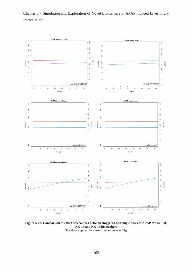
Chapter 5 – Simulation and Exploration of Novel Biomarkers in APAP induced Liver Injury
Introduction
162
Figure 5-18: Comparison of effect timecourses between staggered and single doses of APAP for GLDH,
AK-18 and NK-18 biomarkers
The dose applied for these simulations was 64g

Chapter 5 – Simulation and Exploration of Novel Biomarkers in APAP induced Liver Injury
Introduction
163
5.3.4. ROC –AUC Results for Novel Biomarkers
In the ROC-AUC analysis, ROC-AUC for GLDH and miR-122 increases from its initial value
at time zero, plateauing at 20 hours and 5 hours, respectively (Figure 5-19), with the ROC-
AUC for GLDH increasing slightly again from 65 to 70 hours. The ROC-AUC for HMGB1,
AK-18 and NK-18 levels did not change over the investigated time course of 72 hours (Figure
5-19), being close to 1 throughout the time course for both HMGB1 and AK-18.
Figure 5-19: ROC-AUC for novel biomarkers across a rich timepoint profile.
The black line for HMGB1, red line for miR-122, blue line for GLDH, orange line for AK-18 and green line for
NK-18.

Chapter 5 – Simulation and Exploration of Novel Biomarkers in APAP induced Liver Injury
Introduction
164
5.3.5. ROC Analysis for Novel Biomarkers PKPD Parameter Estimates
An ROC-AUC close to 1 indicates the parameter in question is a potentially accurate predictor
of DILI. Statistical significance was tested vs. a null hypothesis of the ROC-AUC being equal
to 0.5 (which indicates the accuracy of the predictor is no better than random chance) with
statistical significance considered at a P-value < 0.05.
5.3.5.1. ROC Analysis for pharmacokinetic parameters
Table 5-3: Clearance-ROC statistical analysis for pharmacokinetic parameters.
Parameters ROC-AUC P-value Specificity Sensitivity
Cl 0.67 0.9 0.8 0.5
5.3.5.2. ROC Analysis for pharmacodynamic parameters
5.3.5.2.1. HMGB1
Table 5-4: HMGB1-ROC statistical analysis for pharmacodynamic parameters.
Parameters ROC-AUC P-value Specificity Sensitivity
Ke0 0.69 0.99 0.85 0.4375
Kin 0.75 0.000791 0.62 0.875
Kout 0.90 1 0.92 0.9375
Emax 0.81 < 0.0001 0.64 0.875
EC50 0.33 0.99 0.012 1
E0 0.96 < 0.0001 0.91 1
AUCBiomarker 0.97 < 0.0001 0.91 1
t1/2 0.90 < 0.0001 0.92 0.937

Chapter 5 – Simulation and Exploration of Novel Biomarkers in APAP induced Liver Injury
Introduction
165
5.3.5.2.2. miR-122
Table 5-5: miR-122-ROC statistical analysis for the pharmacodynamic parameters.
Parameters ROC-AUC P-value Specificity Sensitivity
Ke0 0.68 0.01 0.41 0.93
Kin 0.63 0.95 1 0.37
Kout 0.93 1 0.87 0.93
Emax 0.85 < 0.0001 0.83 0.75
EC50 0.84 0.99 0.65 0.93
E0 0.89 < 0.0001 0.87 0.87
AUCBiomarker 0.97 < 0.0001 0.97 0.87
t1/2 0.93 < 0.0001 0.87 0.93
5.3.5.2.3. GLDH
Table 5-6: GLDH-ROC statistical analysis for the pharmacodynamic parameters.
Parameters ROC-AUC P-value Specificity Sensitivity
Ke0 0.64 0.96 0.96 0.43
Kin 0.68 0.01 0.57 0.81
Kout 0.67 0.98 0.98 0.56
Emax 0.88 < 0.0001 0.98 0.68
EC50 0.74 0.99 0.52 0.87
E0 0.75 0.0006 0.66 0.81
AUCBiomarker 0.97 < 0.0001 0.97 0.87
t1/2 0.67 0.013 0.98 0.56
5.3.5.2.4. AK-18
Table 5-7: AK-18-ROC statistical analysis for the pharmacodynamic parameters.
Parmeters ROC-AUC P-value Specificity Sensitivity
Ke0 0.53 0.33 0.78 0.56
Kin 0.79 0.0001 0.93 0.62
Kout 0.97 1 0.88 1
Emax 0.76 0.0004 0.89 0.62
EC50 0.80 0.99 0.93 0.75
E0 0.97 < 0.0001 0.89 1
AUCBiomarker 0.97 < 0.0001 0.89 1
t1/2 0.97 < 0.0001 0.88 1

Chapter 5 – Simulation and Exploration of Novel Biomarkers in APAP induced Liver Injury
Introduction
166
5.3.5.2.5. NK-18
Table 5-8: NK-18-ROC statistical analysis for the pharmacodynamic parameters.
Parameters ROC-AUC P-value Specificity Sensitivity
Ke0 0.77 0.99 0.89 0.625
Kin 0.86 < 0.0001 0.93 0.68
Kout 0.97 1 0.93 1
Emax 0.87 < 0.0001 0.92 0.75
EC50 0.73 0.001 0.92 0.62
E0 0.97 < 0.0001 0.93 1
AUCBiomarker 0.97 < 0.0001 0.94 1
t1/2 0.97 < 0.0001 0.93 1

Chapter 5 – Simulation and Exploration of Novel Biomarkers in APAP induced Liver Injury
Introduction
167
5.4. Discussion
A primary aim of this chapter was to explore which novel biomarker could potentially be the
earliest to detect liver injury post APAP overdose and additionally to investigate the change in
time course effect profile for each biomarker at different doses and dosing frequency.
The simulations of the different biomarker time course effect profiles suggest that NK-18 is
the only biomarker among those investigated in this study to show a clearly detectable, dynamic
response above its normal range, on a 72h timescale (that may in turn be indicative of liver
injury). This is particularly illustrated in Figure 5-11 which shows that compared to the gold
standard biomarker ALT, NK-18 levels start to increase above normal range < 4h post APAP
overdose ingestion, whereas ALT levels remain constant and within the normal range over 72h.
These simulations clarify and are consistent with a visual examination of the raw data used for
the modelling (reference the VPCs for NK-18 and ALT in chapter 4).
Furthermore NK-18 was also the only biomarker to show dose dependent changes in its levels
under simulations with different doses of APAP. Simulations also showed that a 64g dose
whether given as a single dose or staggered as 4 doses at 2h intervals gave similar levels of
NK-18. For all the other biomarkers, simulations showed no dose dependent changes in levels
and again no changes between a staggered vs. a non-staggered regimen.
In general, in the BIOPAR study dataset biomarker levels in most patients over a 72h interval
tended to fall within normal ranges, with timecourses relatively flat in shape, except those for
NK-18. This is despite all the patients having overdosed and there being a wide range of dose
levels (from 8g to ~150g, typical dose (mean) 33g) among them i.e. the data for biomarkers
except NK-18 is flat and within normal range for most patients irrespective of whether they
took a high, typical or low overdose. In retrospect it is not surprising therefore that the modelled
fits to the data for most of the biomarkers describe flat profiles with little dose dependence in
response. It could be speculated that this may be partially due to the protective effect of NAC
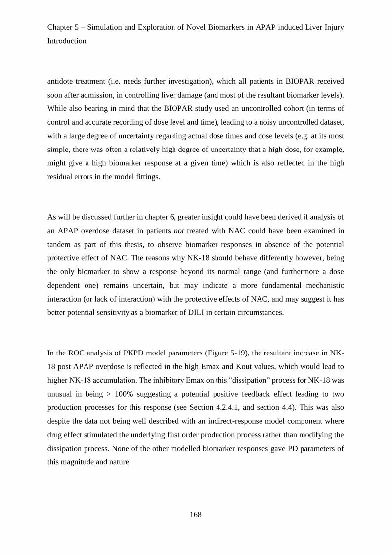
Chapter 5 – Simulation and Exploration of Novel Biomarkers in APAP induced Liver Injury
Introduction
168
antidote treatment (i.e. needs further investigation), which all patients in BIOPAR received
soon after admission, in controlling liver damage (and most of the resultant biomarker levels).
While also bearing in mind that the BIOPAR study used an uncontrolled cohort (in terms of
control and accurate recording of dose level and time), leading to a noisy uncontrolled dataset,
with a large degree of uncertainty regarding actual dose times and dose levels (e.g. at its most
simple, there was often a relatively high degree of uncertainty that a high dose, for example,
might give a high biomarker response at a given time) which is also reflected in the high
residual errors in the model fittings.
As will be discussed further in chapter 6, greater insight could have been derived if analysis of
an APAP overdose dataset in patients not treated with NAC could have been examined in
tandem as part of this thesis, to observe biomarker responses in absence of the potential
protective effect of NAC. The reasons why NK-18 should behave differently however, being
the only biomarker to show a response beyond its normal range (and furthermore a dose
dependent one) remains uncertain, but may indicate a more fundamental mechanistic
interaction (or lack of interaction) with the protective effects of NAC, and may suggest it has
better potential sensitivity as a biomarker of DILI in certain circumstances.
In the ROC analysis of PKPD model parameters (Figure 5-19), the resultant increase in NK-
18 post APAP overdose is reflected in the high Emax and Kout values, which would lead to
higher NK-18 accumulation. The inhibitory Emax on this “dissipation” process for NK-18 was
unusual in being > 100% suggesting a potential positive feedback effect leading to two
production processes for this response (see Section 4.2.4.1, and section 4.4). This was also
despite the data not being well described with an indirect-response model component where
drug effect stimulated the underlying first order production process rather than modifying the
dissipation process. None of the other modelled biomarker responses gave PD parameters of
this magnitude and nature.

Chapter 5 – Simulation and Exploration of Novel Biomarkers in APAP induced Liver Injury
Introduction
169
ROC analysis of the various biomarkers suggests that HMGB1, AK-18 and NK-18 are accurate
predictors of liver injury across all the investigated timepoints across a 72h interval post
overdose as indicated by each of these biomarkers showing an ROC-AUC close to 1 for all
timepoints through 72h.
miR-122 shows an improvement in its ROC-AUC from 0.87 at 0h to 0.90 by 5h and continues
to rise in value to 0.93 by 72h, which suggests that later timepoints for this biomarker are more
predictive for this biomarker.
GLDH also shows improvement in its ROC-AUC over 72h, with a plateau in overall prediction
quality after 20h, however GLDH is apparently the least predictive of all the biomarkers
examined (maximum ROC-AUC of 0.89).
Regarding the prediction of DILI outcome using PKPD model parameters, pharmacokinetic
clearance of APAP (CL, reflecting dose normalised exposure) was not shown to be statistically
significant. Among the pharmacodynamic parameter estimates, the AUC-biomarker was the
best parameter prediction for HMGB1, miR-122 and GLDH.
Clinical application of these biomarkers to identify and stratify APAP overdose patients as to
whether they have liver injury or not could be promising, yet, needs further investigation.
Caution must be taken with the ROC analysis given the limitations of the BIOPAR dataset in
this context i.e. its uncertainties regarding both patient dose levels and dose times, and that
most of the observed biomarkers were within their normal ranges. The resultant individual
patient model fits, parameter estimates and simulations from this data will carry forward these
uncertainties and errors which in turn will propagate into the ROC analysis. Therefore,
although a particular biomarker in this analysis may have a ROC-AUC close to one for its
levels throughout its 72h timecourse, and/or for one or more of its summary PKPD model

Chapter 5 – Simulation and Exploration of Novel Biomarkers in APAP induced Liver Injury
Introduction
170
parameters (e.g. AK-18, HMGB1) this should not be interpreted as a clear, unambiguously
significant result regarding it’s potential clinical utility. Rather, the relatively poor underlying
data should be a major consideration and the findings here regarded as more of an initial
indication of their potential use either diagnostically, or even perhaps in personalisation of
treatment (e.g. dose of NAC antidote therapy).
Further caveats should also be noted regarding the ROC analysis itself, for example when we
analyse a biomarker in this manner, consideration is effectively given regarding the incidence
(new finding) and prevalence (present finding) of the effect. In the case of idiosyncratic DILI
where the outcome event is relatively rare an ROC analysis might not as effectively judge the
diagnostic utility of a biomarker. This is shown particularly in the BIOPAR dataset where only
16 had ALT >100 IU and had consider clinical DILI compared with 78 who had ALT <100
and were not clinical DILI.

Chapter 6 –Conclusion and Further Direction
171
Chapter 6:
Conclusions and Further
Directions

Chapter 6 –Conclusion and Further Direction
172
Chapter 6. Conclusions and Further Directions
This thesis is focused on developing pharmacometrics and statistical methods that can be
applied to novel biomarker data to predict early detection of liver injury in patients with APAP
overdose.
The previous chapters have explored different methods used in approaching this research and in
this conclusion chapter, a brief overview about the research and the results will be provided with
emphasis on the potential limitations that were faced during analysis. Where applicable,
recommendations for how to replicate the approaches taken will be made as references for future
research. Finally, potential future work is discussed where the research of this thesis could be
extended.
6.1. Overview
APAP is a widely used over-the-counter (OTC) medication and APAP overdose is a major
medical problem in the UK and one of the leading causes of drug induced liver injury and acute
liver failure [2]. Stratification of risk and the need for N-acetyl-cysteine (NAC) antidote
therapy is sub-optimal and based on a timed plasma APAP concentration. NAC therapy is
extremely effective but its protective effects decline substantially if dosed 8 hours after an
APAP overdose ingestion. NAC protects the liver and other tissues (e.g. kidney) by
maintaining or restoring glutathione (GTH) levels, and by acting as alternate substrate for
NAPQI metabolism to allow NAPQI to be converted into inactive metabolite [178].
Liver dysfunction from APAP toxicity is initially identified and monitored by evaluating
aspartate aminotransferase (AST) and alanine aminotransferase (ALT) [179], with both
biomarkers being widely assayed in routine hospital laboratories at relatively low cost. In
clinical research ALT is the more commonly discussed biomarker, and serum ALT
concentration of > 100 IU/L is defined as indicating liver injury whereas a value 1000 IU/L is
defined to indicate hepatotoxicity e.g. after APAP overdose[180]. Both biomarkers however
lack sensitivity and specificity to detect DILI post APAP overdose especially for example as
Chapter 6 –Conclusion and Further Direction
173
ALT levels could also be elevated in other hepatic and non-hepatic conditions in addition to
DILI [63] [64].
Mechanistic biomarkers have been demonstrated to provide added value for the early
prediction of APAP-induced hepatotoxicity [81]. Biomarkers of this type include HMGB1,
miR-122, GLDH, AK-18 and NK-18 These biomarkers can be quantified at the earliest
possible time point following admission to hospital and their potential sensitivity to make a
decision regarding early exclusion of liver injury could reduce hospital occupation or unwanted
adverse reactions such as skin rash from unnecessary NAC treatment.
Despite the large quantity of research on APAP overdose, its treatment and its biomarkers there
is still insufficient information about patient safety, treatment and prediction/ prognosis for
patient outcome. Treatment decisions are predominantly based on dose of APAP and a timed
serum APAP concentration, however, patients’ clinical stress often leads to an incomplete
history regarding the amount and time of an APAP overdose that could lead to potential
overtreatment in some patients with what is a potentially harmful antidote with serious side
effects (e.g. nausea, vomiting and skin rash), or perhaps more seriously a lack of treatment
when it is actually needed.
Population pharmacokinetic/pharmacodynamic (Pop-PKPD) approaches have been developed
to bridge the gap between laboratory and clinic using computational models. In this thesis, Pop-
PKPD was deployed to fit mathematical models to novel clinical biomarker data from the
BIOPAR trial for liver injury prediction post APAP overdose. Findings from this analysis could
help with stratifying patients in terms of liver injury, with potential useful clinical application
in individualisation of patient antidote therapy.
In Chapter 3, a Pop-PK model was developed to estimate patient pharmacokinetic parameters,
such as clearance and volume of distribution. A one compartment model with first order
absorption with an exponential residual error model was chosen as the most appropriate model
for the data fitting. The effects of the covariates (weight, age, gender, alcoholism and liver
Chapter 6 –Conclusion and Further Direction
174
injury biomarkers; ALT and INR) were evaluated in the final model. Only alcoholism status
was a significant covariate, with alcoholic patients having a 14% increase in APAP clearance
compared to non-alcoholic patients. It was also an important finding from this dataset that the
typical APAP clearance following an overdose is lower (by approximately 50%) than that seen
following a therapeutic dose, which could potentially be due to liver injury or the transient
insult of the APAP overdose itself.
In chapter 4, a sequential PKPD modelling approach was taken with the novel DILI biomarker
data, using a combined effect compartment/indirect effect model that was implemented to
describe the time course effect of APAP overdose on current and novel biomarkers, with an
initial aim of this approach being to help in early prediction of liver injury. In the BIOPAR
study, measured biomarker levels in most patients tended to fall within normal ranges, with
time-courses relatively flat in shape, and the PKPD models yielded parameter estimates
reflecting these trends in the data. This flat shape could be due to the protective effect of NAC
which was administered to patients soon upon their admission to hospital. Only the NK-18
biomarker showed dynamic deviation above its normal range suggesting its potential greater
sensitivity as a diagnostic tool for DILI following overdose.
Further steps were taken using parameter estimates from this analysis in Chapter-5 (section
5.3.1) for simulation of clinical scenarios to investigate early detection of DILI after an APAP
overdose liver insult, using novel biomarkers. In addition an ROC analysis was used (section
5.3.5) to investigate the ability of various indices from these analyses and simulations to predict
DILI in a patient as defined by their having a peak ALT >100 U/L. The ROC analysis for
biomarker levels simulated at various timepoints showed good potential predictivity for
HMGB1 and AK18 biomarkers measured at any timepoint across a 72h timecourse following
overdose. When analysing individual PKPD model parameters, Biomarker AUC generally
showed the best ability to predict DILI, and perhaps surprisingly APAP-CL (reflecting APAP
PK exposure) did not show very good predictive capacity. This may reflect a greater degree of
variability in the liver PD response to overdose and may also be reflected in the lack of clear
dose-response observed and simulated for the biomarker responses. This assessment of the
potential utility of these biomarkers must however be considered with the caveat of the quality
of the dataset and model fittings on which they were based.

Chapter 6 –Conclusion and Further Direction
175
6.2. Limitations and Recommendations for future research in DILI with
novel biomarkers
The approaches taken in this work represent a toxicological application of pharmacometrics,
which might be defined as “Population pharmacotoxicology”. Due to ethical issues (e.g. that
we cannot give a toxic dose to any person who will enrol into a controlled study, the critical
psychological status for patients that overdose) the data for this form of analysis is inherently
uncontrolled and limited, which will limit this analytical approach in general. Analysis would
be assisted by more appropriate control data with rich sampling and n-numbers, where there
was control over dose time and dose level. However even if it existed this control data would
only ever be available at a therapeutic dose, which may limit how it would assist analysis of
data at a toxic dose.
There are various limitations that should be acknowledged with the work in this thesis. For
example it should be noted that the developed Pop-PK model is hindered by the large degree
of uncertainty regarding actual dose times and dose levels of APAP, combined with the sparse
and uncontrolled sampling schedule. There was also no information available regarding details
of other parallel treatments for overdose e.g. administration of single dose activated charcoal
(SDAC), or use and timing of stomach pumping both of which could potentially have marked
influence on PK and PD profiles. The data has been modelled based on the information given
however, so errors in this dosing record are likely to explain the high residual error of the model
and the relatively poor accounting of interindividual variability by the other random effects
components of the model fits to each set of biomarker data. To remedy these issues would
require a better controlled study that would precisely collect patients’ samples at defined
timepoints, however, controlling the dose-level administered would not be possible in an
overdose scenario dataset.
In general it was also the case that almost no covariate effects were identified in this PKPD
analysis – the only significant covariate effect of potential clinical significance was a PK effect
of alcoholism status on CL. No significant covariate effects were identified in the biomarker
PKPD analysis: for example no clear covariate relationships were identified between PD
parameters describing liver injury as assessed by biomarkers and APAP clearance/exposure in

Chapter 6 –Conclusion and Further Direction
176
this dataset, or alcoholism status. This was perhaps due to the dataset homogeneity (i.e. all
patients were overdose patients and all received NAC antidote therapy) and the relatively small
number of patients in the dataset (i.e. insufficient statistical power to identify potential
covariate effects).
A further limitation of this study is the lack of control groups to provide context and comparison
for the data from the overdose patients. A dataset in patients receiving a therapeutic dose would,
for example, provide a better characterization of potential dose-response of the biomarkers,
and also the parameters of the effect compartment component of the overall combined PD
model (as previously demonstrated in the analysis of Gibb and Anderson.[166]). Further, a
control/comparison dataset with patients not receiving NAC treatment would afford the ability
to compare the difference in biomarker responses, and potentially differences in PK and APAP
exposure, in the absence of NAC. This could for example help to identify if a clearer and more
dynamic biomarker response over time could be seen with biomarkers other than NK-18.
Beyond assessing diagnostic biomarkers of DILI, Pop-PK/PKPD modelling of the form
described in this thesis has the potential to help with NAC antidote dose personalisation.
Initially this could use the understanding of the Pop-PK of APAP itself to individualise the
NAC dose according to APAP exposure (e.g. with precedent based on the work of Duffull 2013
[181] where the total dose of APAP was shown to predict if NAC treatment was required).
This form of recommendation could be refined if it was extended by inclusion of PKPD
analysis of DILI biomarker data to identify relationships between NAC therapy and biomarker
responses. Further refinement still would be gained if GTH and NAPQI levels could be
quantified and modelled in parallel with APAP exposure and DILI biomarker data.
Quantification of GTH would potentially allow a more mechanistic PKPD relationship to be
characterised for the biomarker responses, perhaps incorporating consideration of the NAPQI
intermediate as part of the model. Obviously, however, a much better controlled and higher
quality PKPD dataset than that available from the BIOPAR trial, observing PK and PD at
varying doses (or even presence/absence) of NAC would be required to develop such
approaches.

Chapter 6 –Conclusion and Further Direction
177
If a more detailed form of analysis such as this could be achieved however, the NAC dose
individualisation itself would be able to make use of techniques developed for target
concentration intervention (TCI), a long established strategy for individualised therapy [182]
where the fundamental knowledge provided by combination PKPD models to describe the time
course for drug response can be useful. TCI is a rational approach to achieve a desired clinical
outcome based on drug effect and concentration observations to select the best dose to achieve
the therapeutic effect [183] and is an expansion of the knowledge of therapeutic drug
monitoring (TDM) [184].
The target concentration provides a balance between therapeutic effects and adverse effects
(e.g. adverse effects for NAC treatment include nausea, vomiting and skin rash). TCI is
different from therapeutic drug monitoring (TDM) in that TCI aims for a single target
concentration while TDM aims for a range of concentrations in a “therapeutic window”. A
single target might be expected to have a better balance between the drug beneficial and adverse
effects, while a TDM derived concentration range may be less than optimal with more
noticeable adverse effects at the top end of the concentration range. Pop-PD models describe
concentration effect relationships rather than to identify a clinical endpoint or target effect (TE)
[185]. The target concentration (TC) can be predicted from the Emax PD model if the TE is
known by using Equation 6-1.
TC = (C50 * TE)/(Emax –TE) Equation 6-1
This TE method was applied previously for theophylline in treatment of asthma, with TE based
on the peak expiratory flow rate (PEFR) as the clinical endpoint [186]. However, here it would
be applied to NAC dosing based on a PKPD understanding of its interactions and effects on
the biomarkers of DILI, making specific use of PKPD model parameter estimates to tailor
dosing (loading, maintenance infusions etc.) according to standard PK equations.
Biomarker PKPD analysis of the form used in this work could also be implemented with data
on a long timecourse (should this become available) to then make use of methods described by

Chapter 6 –Conclusion and Further Direction
178
Holford for disease progression modelling which could be implemented to stratify liver injured
patients into three groups; liver injury recovered, liver transplant and dead on a longer timescale
[187]. The disease progression refers to the time course of the changes in the disease under the
influence of an ingested drug (in this case overdosed APAP). Disease status refers then to any
quantifiable variable to describe disease at a particular point in time; it can also be defined as a
clinical outcome such as survival or symptoms, or be measured with a biomarker which can be
used by clinicians as diagnostic or prognostic variables.
The TCI and disease progression modelling methodologies therefore have potential for
application to individualization of therapy following APAP overdose and prediction of long
term liver injury outcome. However, a large investment in future research to characterize the
PKPD of NAC therapy itself will be required, i.e. quantifying biomarker responses following
APAP administration (or insult) but with varying treatment doses of NAC antidote therapy,
and ideally with additional quantification of GTH and NAPQI for greater mechanistic
understanding.
If such datasets could be obtained they would require analysis by the PKPD methods described
and applied in this thesis for the BIOPAR trial, yielding similar forms of results but with a
focus on the effect of antidote treatment. If sufficiently characterized by this analytical process,
the findings from this future work could be used in both TCI and disease progression modelling
frameworks to specify the most beneficial dosing regimen(s) for NAC antidote therapy,
balancing therapeutic effects and the likelihood of a good outcome, with safety and side effects.
TCI models become useful in clinical situations by providing methods that are accessible,
include checks for accurate input of patient data, and provide output in the form of proposed
doses and dosing intervals potentially as well as plots of predicted concentrations in relation to
the target concentration. The potential benefit of TCI methods are therefore that the desired
therapeutic targets can be reached by using a more straightforward calculation of dose with less
potential error, combined with the convenience of a web tool or software that is easy to access
for use anywhere with internet access.

Chapter 6 –Conclusion and Further Direction
179
The approaches outlined in this thesis therefore could be used in the future with overdose
patients presenting at hospital with a suspected APAP overdose to determine their probability
of DILI. Identifying if the liver is healthy in DILI could minimise patient stays in hospital,
prevent adverse effects and save money by identifying patients who do not need to be treated,
in addition follow up could be reduced and better opportunities given for others who genuinely
need treatment to stay at hospital.

References
180
References
1. Jozwiak-Bebenista, M. and J.Z. Nowak, Paracetamol: mechanism of action,
applications and safety concern. Acta Pol Pharm, 2014. 71(1): p. 11-23.
2. Schiodt, F.V., et al., Etiology and outcome for 295 patients with acute liver failure in
the United States. Liver Transpl Surg, 1999. 5(1): p. 29-34.
3. Mowry, J.B., et al., 2014 Annual Report of the American Association of Poison Control
Centers' National Poison Data System (NPDS): 32nd Annual Report. Clin Toxicol
(Phila), 2015. 53(10): p. 962-1147.
4. Bateman, D.N., et al., Effect of the UK's revised paracetamol poisoning management
guidelines on admissions, adverse reactions and costs of treatment. Br J Clin
Pharmacol, 2014. 78(3): p. 610-8.
5. Statistics, O.f.N., Deaths Related to Drug Poisoning, England and Wales. 2017: UK.
6. Zyoud, S.e.H., et al., The 100 most influential publications in paracetamol poisoning
treatment: a bibliometric analysis of human studies. SpringerPlus, 2016. 5(1): p. 1534.
7. Bertolini, A., et al., Paracetamol: new vistas of an old drug. CNS Drug Rev, 2006.
12(3-4): p. 250-75.
8. Brodie, B.B. and J. Axelrod, The fate of acetanilide in man. J Pharmacol Exp Ther,
1948. 94(1): p. 29-38.
9. Nancy West Communications, Worldwide Consumer Pharmaceutical Intranet Site:
"History of TYLENOL". 2018: Washington DC.
10. Jiben, R., The Top Five Most Common or Long-Selling Drugs, in An Introduction to
Pharmaceutical Sciences "Production, Chemistry, Techniques and Technology". 2011,
WoodHead Publishing. p. 270.
11. BNF, Paracetamole. 2018, National Institute for Health and Care Excellence.
12. Bromer, M.Q. and M. Black, Acetaminophen hepatotoxicity. Clin Liver Dis, 2003. 7(2):
p. 351-67.
13. Fagan, E. and G. Wannan, Reducing paracetamol overdoses. BMJ, 1996. 313(7070):
p. 1417-8.
14. Larson, A.M., Acetaminophen hepatotoxicity. Clin Liver Dis, 2007. 11(3): p. 525-48,
vi.
15. Civan, J.M., et al., Patterns of Acetaminophen Use Exceeding 4 Grams Daily in a
Hospitalized Population at a Tertiary Care Center. Gastroenterology & Hepatology,
2014. 10(1): p. 27-34.
16. Levy, G., Comparative pharmacokinetics of aspirin and acetaminophen. Arch Intern
Med, 1981. 141(3 Spec No): p. 279-81.
17. Milligan, T.P., et al., Studies on paracetamol binding to serum proteins. Ann Clin
Biochem, 1994. 31 ( Pt 5): p. 492-6.
18. Gelotte, C.K., et al., Disposition of acetaminophen at 4, 6, and 8 g/day for 3 days in
healthy young adults. Clinical Pharmacology & Therapeutics, 2007. 81(6): p. 840-848.
19. Danielson, P.B., The cytochrome P450 superfamily: biochemistry, evolution and drug
metabolism in humans. Curr Drug Metab, 2002. 3(6): p. 561-97.
20. Moffit, J.S., et al., Role of NAD(P)H:quinone oxidoreductase 1 in clofibrate-mediated
hepatoprotection from acetaminophen. Toxicology, 2007. 230(2-3): p. 197-206.
21. Prescott, L.F., Kinetics and metabolism of paracetamol and phenacetin. Br J Clin
Pharmacol, 1980. 10 Suppl 2: p. 291S-298S.
22. Aronoff, D.M., J.A. Oates, and O. Boutaud, New insights into the mechanism of action
of acetaminophen: Its clinical pharmacologic characteristics reflect its inhibition of the
References
181
two prostaglandin H2 synthases. Clinical Pharmacology & Therapeutics, 2006. 79(1):
p. 9-19.
23. Dubois, R.N., et al., Cyclooxygenase in biology and disease. FASEB J, 1998. 12(12):
p. 1063-73.
24. Seibert, K., et al., Pharmacological and biochemical demonstration of the role of
cyclooxygenase 2 in inflammation and pain. Proc Natl Acad Sci U S A, 1994. 91(25):
p. 12013-7.
25. Pini, L.A., M. Sandrini, and G. Vitale, The antinociceptive action of paracetamol is
associated with changes in the serotonergic system in the rat brain. European Journal
of Pharmacology, 1996. 308(1): p. 31-40.
26. Botting, R. and S.S. Ayoub, COX-3 and the mechanism of action of
paracetamol/acetaminophen. Prostaglandins Leukotrienes and Essential Fatty Acids,
2005. 72(2): p. 85-87.
27. Bjorkman, R., et al., Acetaminophen Blocks Spinal Hyperalgesia Induced by Nmda and
Substance-P. Pain, 1994. 57(3): p. 259-264.
28. Thomson, J.S. and L.F. Prescott, Liver damage and impaired glucose tolerance after
paracetamol overdosage. Br Med J, 1966. 2(5512): p. 506-7.
29. Hawton, K., et al., Why patients choose paracetamol for self poisoning and their
knowledge of its dangers. BMJ : British Medical Journal, 1995. 310(6973): p. 164-164.
30. Sheen, C.L., et al., Paracetamol-related deaths in Scotland, 1994-2000. Br J Clin
Pharmacol, 2002. 54(4): p. 430-2.
31. Hawkins, L.C., J.N. Edwards, and P.I. Dargan, Impact of restricting paracetamol pack
sizes on paracetamol poisoning in the United Kingdom: a review of the literature. Drug
Saf, 2007. 30(6): p. 465-79.
32. Flanagan, R.J. and C. Rooney, Recording acute poisoning deaths. Forensic Sci Int,
2002. 128(1-2): p. 3-19.
33. Morgan, O. and A. Majeed, Restricting paracetamol in the United Kingdom to reduce
poisoning: a systematic review. J Public Health (Oxf), 2005. 27(1): p. 12-8.
34. Hawton, K., et al., Long term effect of reduced pack sizes of paracetamol on poisoning
deaths and liver transplant activity in England and Wales: interrupted time series
analyses. BMJ, 2013. 346: p. f403.
35. Lee, W.M., Drug-induced hepatotoxicity. N Engl J Med, 2003. 349(5): p. 474-85.
36. Jaeschke, H., M.R. McGill, and A. Ramachandran, Oxidant stress, mitochondria, and
cell death mechanisms in drug-induced liver injury: lessons learned from
acetaminophen hepatotoxicity. Drug Metab Rev, 2012. 44(1): p. 88-106.
37. Boyer, T.D. and S.L. Rouff, Acetaminophen-induced hepatic necrosis and renal
failure. JAMA, 1971. 218(3): p. 440-441.
38. Hinson, J.A., et al., Nitrotyrosine-protein adducts in hepatic centrilobular areas
following toxic doses of acetaminophen in mice. Chem Res Toxicol, 1998. 11(6): p.
604-7.
39. Hanawa, N., et al., Role of JNK translocation to mitochondria leading to inhibition of
mitochondria bioenergetics in acetaminophen-induced liver injury. J Biol Chem, 2008.
283(20): p. 13565-77.
40. Kon, K., et al., Mitochondrial permeability transition in acetaminophen-induced
necrosis and apoptosis of cultured mouse hepatocytes. Hepatology, 2004. 40(5): p.
1170-9.
41. Elmore, S., Apoptosis: a review of programmed cell death. Toxicol Pathol, 2007. 35(4):
p. 495-516.

References
182
42. Antoine, D.J., et al., Diet restriction inhibits apoptosis and HMGB1 oxidation and
promotes inflammatory cell recruitment during acetaminophen hepatotoxicity. Mol
Med, 2010. 16(11-12): p. 479-90.
43. Gujral, J.S., et al., Mode of cell death after acetaminophen overdose in mice: apoptosis
or oncotic necrosis? Toxicol Sci, 2002. 67(2): p. 322-8.
44. Malhi, H., G.J. Gores, and J.J. Lemasters, Apoptosis and necrosis in the liver: a tale of
two deaths? Hepatology, 2006. 43(2 Suppl 1): p. S31-44.
45. Robertson, J.D. and S. Orrenius, Molecular mechanisms of apoptosis induced by
cytotoxic chemicals. Crit Rev Toxicol, 2000. 30(5): p. 609-27.
46. Possamai, L.A., et al., Character and Temporal Evolution of Apoptosis in
Acetaminophen-Induced Acute Liver Failure. Critical care medicine, 2013. 41(11): p.
2543-2550.
47. Antoine, D.J., D.P. Williams, and B.K. Park, Understanding the role of reactive
metabolites in drug-induced hepatotoxicity: state of the science. Expert Opin Drug
Metab Toxicol, 2008. 4(11): p. 1415-27.
48. Iorga, A., L. Dara, and N. Kaplowitz, Drug-Induced Liver Injury: Cascade of Events
Leading to Cell Death, Apoptosis or Necrosis. Int J Mol Sci, 2017. 18(5).
49. McGill, M.R., et al., Acetaminophen-induced liver injury in rats and mice: Comparison
of protein adducts, mitochondrial dysfunction, and oxidative stress in the mechanism
of toxicity. Toxicology and Applied Pharmacology, 2012. 264(3): p. 387-394.
50. Jaeschke, H., et al., Current issues with acetaminophen hepatotoxicity—A clinically
relevant model to test the efficacy of natural products. Life Sciences, 2011. 88(17): p.
737-745.
51. Adams, D.H., et al., Mechanisms of immune-mediated liver injury. Toxicol Sci, 2010.
115(2): p. 307-21.
52. Ishida, Y., et al., A pivotal involvement of IFN-gamma in the pathogenesis of
acetaminophen-induced acute liver injury. FASEB J, 2002. 16(10): p. 1227-36.
53. Ju, C. and T. Reilly, Role of immune reactions in drug-induced liver injury (DILI). Drug
Metab Rev, 2012. 44(1): p. 107-15.
54. Lancaster, E.M., J.R. Hiatt, and A. Zarrinpar, Acetaminophen hepatotoxicity: an
updated review. Arch Toxicol, 2015. 89(2): p. 193-9.
55. Prescott, L.F., et al., Plasma-paracetamol half-life and hepatic necrosis in patients with
paracetamol overdosage. Lancet, 1971. 1(7698): p. 519-22.
56. MHRA, New simplified guidance on treating paracetamol overdose with intravenous
acetylcysteine including an updated treatment nomogram. 2012, Medicines and
Healthcare products Regulatory Agency.
57. Rumack, B.H., et al., Acetaminophen overdose. 662 cases with evaluation of oral
acetylcysteine treatment. Arch Intern Med, 1981. 141(3 Spec No): p. 380-5.
58. Prescott, K., et al., Detailed analyses of self-poisoning episodes presenting to a large
regional teaching hospital in the UK. Br J Clin Pharmacol, 2009. 68(2): p. 260-8.
59. Daly, F.F., et al., Guidelines for the management of paracetamol poisoning in Australia
and New Zealand--explanation and elaboration. A consensus statement from clinical
toxicologists consulting to the Australasian poisons information centres. Med J Aust,
2008. 188(5): p. 296-301.
60. Kleiner, D.E., et al., Hepatic histological findings in suspected drug-induced liver
injury: systematic evaluation and clinical associations. Hepatology, 2014. 59(2): p.
661-70.
61. Dear, J.W., et al., Risk stratification after paracetamol overdose using mechanistic
biomarkers: results from two prospective cohort studies. Lancet Gastroenterol Hepatol,
2018. 3(2): p. 104-113.

References
183
62. Ozer, J., et al., The current state of serum biomarkers of hepatotoxicity. Toxicology,
2008. 245(3): p. 194-205.
63. Dhanwal, D.K., Thyroid disorders and bone mineral metabolism. Indian J Endocrinol
Metab, 2011. 15(Suppl 2): p. S107-12.
64. Lofthus, D.M., et al., Pattern of liver enzyme elevations in acute ST-elevation
myocardial infarction. Coron Artery Dis, 2012. 23(1): p. 22-30.
65. Pettersson, J., et al., Muscular exercise can cause highly pathological liver function
tests in healthy men. British Journal of Clinical Pharmacology, 2008. 65(2): p. 253-259.
66. Antoine, D.J., et al., Are we closer to finding biomarkers for identifying acute drug-
induced liver injury? Biomarkers in Medicine, 2013. 7(3): p. 383-386.
67. Antoine, J.D., et al., Safety biomarkers for drug-induced liver injury current status and
future perspectives. Toxicology Research, 2014(3): p. 75-85.
68. Winter, J., et al., Many roads to maturity: microRNA biogenesis pathways and their
regulation. Nat Cell Biol, 2009. 11(3): p. 228-34.
69. Arrese, M., A. Eguchi, and A. Feldstein, Circulating microRNAs: Emerging
Biomarkers of Liver Disease. Semin Liver Dis 2015. 35(1): p. 043-054.
70. Liang, Y., et al., Characterization of microRNA expression profiles in normal human
tissues. BMC Genomics, 2007. 8: p. 166.
71. Wang, K., et al., Circulating microRNAs, potential biomarkers for drug-induced liver
injury. Proc Natl Acad Sci U S A, 2009. 106(11): p. 4402-7.
72. Starkey Lewis, P.J., et al., Circulating microRNAs as potential markers of human drug-
induced liver injury. Hepatology, 2011. 54(5): p. 1767-1776.
73. Yang, H., et al., The many faces of HMGB1: molecular structure-functional activity in
inflammation, apoptosis, and chemotaxis. J Leukoc Biol, 2013. 93(6): p. 865-73.
74. Bonaldi, T., et al., Monocytic cells hyperacetylate chromatin protein HMGB1 to
redirect it towards secretion. EMBO J, 2003. 22(20): p. 5551-60.
75. Antoine, D.J., et al., High-mobility group box-1 protein and keratin-18, circulating
serum proteins informative of acetaminophen-induced necrosis and apoptosis in vivo.
Toxicol Sci, 2009. 112(2): p. 521-31.
76. Antoine, D.J., et al., Molecular forms of HMGB1 and keratin-18 as mechanistic
biomarkers for mode of cell death and prognosis during clinical acetaminophen
hepatotoxicity. J Hepatol, 2012. 56(5): p. 1070-9.
77. Schmidt, E.S. and F.W. Schmidt, Glutamate dehydrogenase: biochemical and clinical
aspects of an interesting enzyme. Clinica Chimica Acta, 1988. 173(1): p. 43-55.
78. Kravos, M. and I. Malešič, The Role of Glutamate Dehydrogenase Activity in
Development of Neurodegenerative Disorders. World Journal of Neuroscience, 2017.
7(1): p. 181-192
79. Taylor, L. and N.P. Curthoys, Glutamine metabolism: Role in acid-base balance*.
Biochem Mol Biol Educ, 2004. 32(5): p. 291-304.
80. Antoine, D.J., et al., Mechanism-based bioanalysis and biomarkers for hepatic
chemical stress. Xenobiotica, 2009. 39(8): p. 565-77.
81. Antoine, D.J., et al., Mechanistic biomarkers provide early and sensitive detection of
acetaminophen-induced acute liver injury at first presentation to hospital. Hepatology,
2013. 58(2): p. 777-87.
82. Antoine, D.J., Translational and Mechanistic Biomarkers of Drug-Induced Liver Injury
– Candidates and Qualification Strategies, in Drug-Induced Liver Toxicity, M. Chen
and Y. Will, Editors. 2018, Humana Press, New York, NY.
83. Vijayaraj, P., G. Sohl, and T.M. Magin, Keratin transgenic and knockout mice:
functional analysis and validation of disease-causing mutations. Methods Mol Biol,
2007. 360: p. 203-51.

References
184
84. Ku, N.O., et al., The cytoskeleton of digestive epithelia in health and disease. Am J
Physiol, 1999. 277(6 Pt 1): p. G1108-37.
85. Dear, J.W. and D.J. Antoine, Stratification of paracetamol overdose patients using new
toxicity biomarkers: current candidates and future challenges. Expert Review of
Clinical Pharmacology, 2014. 7(2): p. 181-189.
86. Cummings, J., et al., Preclinical evaluation of M30 and M65 ELISAs as biomarkers of
drug induced tumor cell death and antitumor activity. Molecular Cancer Therapeutics,
2008. 7(3): p. 455-463.
87. Wieckowska, A., et al., In vivo assessment of liver cell apoptosis as a novel biomarker
of disease severity in nonalcoholic fatty liver disease. Hepatology, 2006. 44(1): p. 27-
33.
88. Longo, D.M., et al., Refining Liver Safety Risk Assessment: Application of Mechanistic
Modeling and Serum Biomarkers to Cimaglermin Alfa (GGF2) Clinical Trials. Clin
Pharmacol Ther, 2017. 102(6): p. 961-969.
89. Holford, N.H.G. and L.B. Sheiner, Understanding the Dose-Effect Relationship -
Clinical-Application of Pharmacokinetic-Pharmacodynamic Models. Clinical
Pharmacokinetics, 1981. 6(6): p. 429-453.
90. Rowland, M. and T.N. Tozer, Clinical pharmacokinetics : concepts and applications.
1995: Baltimore : Williams & Wilkins.
91. Sakai, J.B., Pharmacokinetics: The Absorption, Distribution, and Excretion of Drugs,
in Practical Pharmacology for the Pharmacy Technician. 2008, Lippincott Williams
and Wilkins.
92. Wagner, J.G., Pharmacokinetics. Annual Review of Pharmacology, 1968. 8: p. 67-&.
93. Wagner, J.G., Pharmacokinetics .10. Introduction to Compartment Models. Drug
Intelligence & Clinical Pharmacy, 1969. 3(9): p. 250-&.
94. Wagner, J.G., History of Pharmacokinetics. Pharmacology & Therapeutics, 1981.
12(3): p. 537-562.
95. Iliadis, A., R. Bruno, and J.P. Cano, Steady-State Dosage Regimen Calculations in
Linear Pharmacokinetics. International Journal of Bio-Medical Computing, 1986.
18(3-4): p. 167-182.
96. Ayres, J.W., et al., Linear and Nonlinear Assessment of Tolmetin Pharmacokinetics.
Research Communications in Chemical Pathology and Pharmacology, 1977. 17(4): p.
583-593.
97. Upton, R.N. and D.R. Mould, Basic Concepts in Population Modeling, Simulation, and
Model-Based Drug Development: Part 3—Introduction to Pharmacodynamic
Modeling Methods. CPT: Pharmacometrics & Systems Pharmacology, 2014. 3(1): p.
88.
98. Greenblatt, D.J. and J.S. Harmatz, Kinetic-Dynamic Modeling in Clinical
Psychopharmacology. Journal of Clinical Psychopharmacology, 1993. 13(4): p. 231-
234.
99. Greenblatt, D.J., et al., Kinetic and Dynamic Study of Intravenous Lorazepam -
Comparison with Intravenous Diazepam. Journal of Pharmacology and Experimental
Therapeutics, 1989. 250(1): p. 134-140.
100. Furchgott, R.F., The pharmacology of vascular smooth muscle. Pharmacol Rev, 1955.
7(2): p. 183-265.
101. Sheiner, L.B., et al., Simultaneous modeling of pharmacokinetics and
pharmacodynamics: application to d-tubocurarine. Clin Pharmacol Ther, 1979. 25(3):
p. 358-71.
102. Greenblatt, D.J., et al., pharmacokinetics, pharmacodynamics, and drug disposition, in
Neurophsycopharmacology: the fifth generation of progress, K.L. Davis, D. Charney,
References
185
and J.T. Coyle, Editors. 2002: Philadelphia: Lippincott, Williams and Wilkins. p. 507-
524.
103. Sharma, A. and W.J. Jusko, Characteristics of indirect pharmacodynamic models and
applications to clinical drug responses. British Journal of Clinical Pharmacology,
1998. 45(3): p. 229-239.
104. Sheiner, L. and D. Verotta, Further notes on physiologic indirect response models.
Clinical Pharmacology & Therapeutics, 1995. 58(2): p. 238-240.
105. Dayneka, N.L., V. Garg, and W.J. Jusko, Comparison of Four Basic Models of Indirect
Pharmacodynamic Responses. Journal of pharmacokinetics and biopharmaceutics,
1993. 21(4): p. 457-478.
106. Tatarinova, T., et al., Two general methods for population pharmacokinetic modeling:
non-parametric adaptive grid and non-parametric Bayesian. Journal of
Pharmacokinetics and Pharmacodynamics, 2013. 40(2): p. 189-199.
107. Ette, E.I. and P.J. Williams, Population pharmacokinetics II: estimation methods. Ann
Pharmacother, 2004. 38(11): p. 1907-15.
108. Jelliffe, R., A. Schumitzky, and M. Van Guilder, Population
pharmacokinetics/pharmacodynamics modeling: parametric and nonparametric
methods. Ther Drug Monit, 2000. 22(3): p. 354-65.
109. Gibbons, J.D., Nonparametric Methods f or Quantitative Analysis. 2nd ed. 1985:
American Sciences Press.
110. Siegel, S. and N.J. Castellan, Non-parametric Statistics for the Behavioural Sciences.
2nd ed. 1988: New York: McGraw-Hill.
111. Whitley, E. and J. Bai, Statistics review 6: Nonparametric methods. Critical Care, 2002.
6(6): p. 509-513.
112. Antic J, et al., Nonparametric Methods: When to use them? Which method to choose?,
in Population Approach Group in Europe. 2009: St. Petersburg, Russia.
113. O'Quigley, J., X. Paoletti, and J. Maccario, Non-parametric optimal design in dose
finding studies. Biostatistics, 2002. 3(1): p. 51-6.
114. Schumitzky, A., The Nonparametric Maximum-Likelihood Approach to
Pharmacokinetic Population Analysis. Simulation in Health Sciences and Services,
1993: p. 95-100.
115. Jelliffe, R., et al., Population pharmacokinetic and dynamic models: Parametric (P)
and nonparametric (NP)approaches. Fourteenth Ieee Symposium on Computer-Based
Medical Systems, Proceedings, 2001: p. 407-412.
116. Davidian, M. and D.M. Giltinan, Nonlinear models for repeated measurement data: An
overview and update. Journal of Agricultural Biological and Environmental Statistics,
2003. 8(4): p. 387-419.
117. spieler, G. and A. Schumitzky, Asymptotic Properties of Extended Least Squares with
Application to Population Pharmacokinetics, in Proceedings of American Statistical
Society. 1993. p. 177-182.
118. Population Pharmacokinetics, in Applied Clinical Pharmacokinetics and
Pharmacodynamics of Psychopharmacological Agents, S.R.P. Michael W. Jann,
Lawrence J. Cohen, Editor. 2016, Springer, 2016. p. 74.
119. Sheiner, L., B. Rosenberg, and K. Melmon, Modeling of individual pharmacokinetics
for computer-aided drug dosage. Comput Biomed Res, 1972. 5(5): p. 411-59.
120. Bonate, P.L., Nonlinear Mixed Effect Models: Theory, in Pharmacokinetic-
Pharmacodynamic Modelling and Simulation, n. Edition, Editor. 2011, Springer. p.
233-301.

References
186
121. Aymanns, C., et al., Review on Pharmacokinetics and Pharmacodynamics and the
Aging Kidney. Clinical Journal of the American Society of Nephrology, 2010. 5(2): p.
314-327.
122. Lindstrom, M.J. and D.M. Bates, Nonlinear Mixed Effects Models for Repeated
Measures Data. Biometrics, 1990. 46(3): p. 673-687.
123. Whiting, B., A.W. Kelman, and J. Grevel, Population Pharmacokinetics - Theory and
Clinical-Application. Clinical Pharmacokinetics, 1986. 11(5): p. 387-401.
124. Sheiner, L.B. and S.L. Beal, Evaluation of methods for estimating population
pharmacokinetics parameters. I. Michaelis-Menten model: routine clinical
pharmacokinetic data. J Pharmacokinet Biopharm, 1980. 8(6): p. 553-71.
125. FDA, Guidance for industry on Population Pharmacokinetics, E. F.a.D.A. U.S.
Department of Health Services, Editor. 1999.
126. Davidian, M. and A. Ronald, The Nonlinear Mixed Effects Model with a Smooth
Random Effects Density. Biometrika, 1993. 80(3): p. 475.
127. Sun, H., et al., Population pharmacokinetics. A regulatory perspective. Clin
Pharmacokinet, 1999. 37(1): p. 41-58.
128. Lindbom, L., J. Ribbing, and E.N. Jonsson, Perl-speaks-NONMEM (PsN)--a Perl
module for NONMEM related programming. Comput Methods Programs Biomed,
2004. 75(2): p. 85-94.
129. Beal, S. and L. Sheiner, “NONMEM Users Guide Part VII: Conditional Estimation
Methods” NONMEM Project Group, San Francisco, 1998.
130. Sheiner, L.B. and S.L. Beal, Evaluation of methods for estimating population
pharmacokinetic parameters. III. Monoexponential model: routine clinical
pharmacokinetic data. J Pharmacokinet Biopharm, 1983. 11(3): p. 303-19.
131. Ette, E.I., et al., Analysis of animal pharmacokinetic data: Performance of the one point
per animal design. Journal of Pharmacokinetics and Biopharmaceutics, 1995. 23(6): p.
551-566.
132. Racine, A., et al., Bayesian Methods in Practice - Experiences in the Pharmaceutical-
Industry. Applied Statistics-Journal of the Royal Statistical Society Series C, 1986.
35(2): p. 93-150.
133. Miller, R., Population Pharmacokinetics, in Principles of Clinical Pharmacology, A.
Atkinson and S.M. Huang, Editors. 2012, Elsevier Inc.
134. Sheiner, L.B. and S.L. Beal, Bayesian Individualization of Pharmacokinetics - Simple
Implementation and Comparison with Non-Bayesian Methods. Journal of
Pharmaceutical Sciences, 1982. 71(12): p. 1344-1348.
135. Keizer, R.J., et al., Pirana and PCluster: a modeling environment and cluster
infrastructure for NONMEM. Comput Methods Programs Biomed, 2011. 101(1): p. 72-
9.
136. Alimian, M., et al., Analgesic effects of paracetamol and morphine after elective
laparotomy surgeries. Anesth Pain Med, 2014. 4(2): p. e12912.
137. Heard, K., et al., Overuse of over-the-counter analgesics by emergency department
patients. Ann Emerg Med, 2006. 48(3): p. 315-8.
138. Toxbase, The primary clinical toxicology database of the National Poisons Information
Service. 2016, National Poisons Information Service.
139. Oliveira, E.J., D.G. Watson, and N.S. Morton, A simple microanalytical technique for
the determination of paracetamol and its main metabolites in blood spots. J Pharm
Biomed Anal, 2002. 29(5): p. 803-9.
140. Boeckmann, A., L. Sheiner, and S. Beal, NONMEM Users Guide - Part V "Introductory
Guide". 2011: University of California at San Francisco.
References
187
141. Chaturvedula, A., Population Pharmacokinetics, in Applied Clinical Pharmacokinetics
and Pharmacodynamics of Psychopharmacological Agents, M.W. Jann, S.R. Penzak,
and L.J. Cohen, Editors. 2016, Springer International Publishing: Cham. p. 71-90.
142. Joerger, M., Covariate pharmacokinetic model building in oncology and its potential
clinical relevance. AAPS J, 2012. 14(1): p. 119-32.
143. Muzic, R.F., Jr. and B.T. Christian, Evaluation of objective functions for estimation of
kinetic parameters. Med Phys, 2006. 33(2): p. 342-53.
144. Byon, W., et al., Establishing Best Practices and Guidance in Population Modeling:
An Experience With an Internal Population Pharmacokinetic Analysis Guidance. CPT:
Pharmacometrics & Systems Pharmacology, 2013. 2(7): p. 1-8.
145. Shiffler, R.E., Maximum Z Scores and Outliers. The American Statistician, 1988. 42(1):
p. 79-80.
146. Efron, B., Bootstrap Methods: Another Look at the Jackknife. Ann. Statist., 1979. 7(1):
p. 1-26.
147. Post, T.M., et al., Extensions to the visual predictive check to facilitate model
performance evaluation. J Pharmacokinet Pharmacodyn, 2008. 35(2): p. 185-202.
148. Owens, K.H., et al., Population pharmacokinetic-pharmacodynamic modelling to
describe the effects of paracetamol and N-acetylcysteine on the international
normalized ratio. Clin Exp Pharmacol Physiol, 2015. 42(1): p. 102-8.
149. Reith, D., et al., Simultaneous Modelling of the Michaelis-Menten Kinetics of
Paracetamol Sulphation and Glucuronidation. Clinical and Experimental
Pharmacology and Physiology, 2009. 36(1): p. 35-42.
150. Iedema JM, I.G., Pillans P Population Pharmacokinetics of Paracetamol in Overdose
in a Single Patient, in PAGANZ. 2011: Auckland, New Zealand.
151. Forrest, J.A.H., J.A. Clements, and L.F. Prescott, Clinical Pharmacokinetics of
Paracetamol. Clinical Pharmacokinetics, 1982. 7(2): p. 93-107.
152. Prescott, L.F., Paracetamol, alcohol and the liver. Br J Clin Pharmacol, 2000. 49(4): p.
291-301.
153. Heard, K.J., Acetylcysteine for acetaminophen poisoning. N Engl J Med, 2008. 359(3):
p. 285-92.
154. Senior, J.R., Alanine aminotransferase: a clinical and regulatory tool for detecting
liver injury-past, present, and future. Clin Pharmacol Ther, 2012. 92(3): p. 332-9.
155. Vliegenthart, A.D., D.J. Antoine, and J.W. Dear, Target biomarker profile for the
clinical management of paracetamol overdose. Br J Clin Pharmacol, 2015. 80(3): p.
351-62.
156. Antoine, D.J., Translational and Mechanistic Biomarkers of Drug-Induced Liver Injury
– Candidates and Qualification Strategies, in Drug-Induced Liver Toxicity, M. Chen
and Y. Will, Editors. 2018, Springer New York: New York, NY. p. 533-553.
157. Applied Biosystems. TaqMan™ Universal PCR Master Mix. 2018 [cited 2018 5th
Fabruary ]; Available from:
https://www.thermofisher.com/order/catalog/product/4304437?SID=srch-srp-
4304437.
158. IBL International. HMGB1 ELISA. 2018 [cited 2018 4th Feb]; Available from:
http://www.ibl-international.com/en/hmgb1.
159. Scientific, F. Thermo Scientific VARIOSKAN FLASH. 2018 [cited 2018 26th Feb];
Available from: https://www.fishersci.co.uk/shop/products/11869540/11869540.
160. Diapharma. M30 Apoptosense® CK18 Kit. 2018 [cited 2018 26th Feb]; Available
from: https://diapharma.com/product/apoptosis/ck18kit/.
161. Diapharma. M65 EpiDeath® CK18 Kit. 2018; Available from:
https://diapharma.com/product/apoptosis/m65-epideath-elisa/.
References
188
162. Scientific, T. Infinity ALT/GPT Reagent. 2018 26th Feb]; Available from:
https://www.thermofisher.com/order/catalog/product/TR18503.
163. Danhof, M., et al., Mechanism-based pharmacokinetic-pharmacodynamic (PK-PD)
modeling in translational drug research. Trends in Pharmacological Sciences, 2008.
29(4): p. 186-191.
164. Danhof, M., et al., Mechanism-based pharmacokinetic-pharmacodynamic modeling -
A new classification of biomarkers. Pharmaceutical Research, 2005. 22(9): p. 1432-
1437.
165. Danhof, M., et al., Mechanism-based pharmacokinetic-pharmacodynamic modeling-a
new classification of biomarkers. Pharm Res, 2005. 22(9): p. 1432-7.
166. Gibb, I.A. and B.J. Anderson, Paracetamol (acetaminophen) pharmacodynamics:
interpreting the plasma concentration. Arch Dis Child, 2008. 93(3): p. 241-7.
167. Cleton, A., et al., Application of a Combined 'Effect Compartment/Indirect Response
Model' to the Central Nervous System Effects of Tiagabine in the Rat. 1999, PLENUM
PUBLISHING CORPORATION: United States. p. 301.
168. Ben-Shachar, R., et al., The biochemistry of acetaminophen hepatotoxicity and rescue:
a mathematical model. Theor Biol Med Model, 2012. 9: p. 55.
169. James, L.P., et al., Pharmacokinetics of acetaminophen-protein adducts in adults with
acetaminophen overdose and acute liver failure. Drug Metab Dispos, 2009. 37(8): p.
1779-84.
170. Hinson, J.A., D.W. Roberts, and L.P. James, Mechanisms of acetaminophen-induced
liver necrosis. Handb Exp Pharmacol, 2010(196): p. 369-405.
171. Thulin, P., et al., Keratin-18 and microRNA-122 complement alanine aminotransferase
as novel safety biomarkers for drug-induced liver injury in two human cohorts. Liver
Int, 2014. 34(3): p. 367-78.
172. Clarke, J., N. Brillant, and D.J. Antoine, Novel circulating- and imaging-based
biomarkers to enhance the mechanistic understanding of human drug-induced liver
injury Journal of Clinical and Translational Research 2017. 3(S1).
173. Kullak-Ublick, G.A., et al., Drug-induced liver injury: recent advances in diagnosis
and risk assessment. Gut, 2017. 66(6): p. 1154-1164.
174. Hajian-Tilaki, K., Receiver Operating Characteristic (ROC) Curve Analysis for
Medical Diagnostic Test Evaluation. Caspian J Intern Med, 2013. 4(2): p. 627-35.
175. Robin, X., et al., pROC: an open-source package for R and S+ to analyze and compare
ROC curves. BMC Bioinformatics, 2011. 12: p. 77.
176. BMJ, BMJ Best Practice: Paracetamol Overdose. 2016: PMJ.
177. Metz, C.E., Basic principles of ROC analysis. Semin Nucl Med, 1978. 8(4): p. 283-98.
178. Ferner, R.E., J.W. Dear, and D.N. Bateman, Management of paracetamol poisoning.
BMJ, 2011. 342: p. d2218.
179. Mowry, J.B., et al., 2012 Annual Report of the American Association of Poison Control
Centers' National Poison Data System (NPDS): 30th Annual Report. Clin Toxicol
(Phila), 2013. 51(10): p. 949-1229.
180. McGovern, A.J., et al., Can AST/ALT ratio indicate recovery after acute paracetamol
poisoning? Clinical Toxicology, 2015. 53(3): p. 164-167.
181. Duffull, S.B. and G.K. Isbister, Predicting the requirement for N-acetylcysteine in
paracetamol poisoning from reported dose. Clin Toxicol (Phila), 2013. 51(8): p. 772-
6.
182. Holford, N.H.G., Target concentration intervention: beyond Y2K. British Journal of
Clinical Pharmacology, 2001. 52: p. 55s-59s.
183. Holford, N.H.G., Target concentration intervention: beyond Y2K. British Journal of
Clinical Pharmacology, 1999. 48(1): p. 9-13.

References
189
184. Holford, N., The clearance and volume method of dose prediction, in Avery's Drug
Treatment: A Guide to the Properties, Choice, Therapeutic Use and Economic Value
of Drugs in Disease Management, N. Holford, T.M. Speight, and G.S. Avery, Editors.
1997, Adis Press: Auckland, N.Z. p. 1791-1798.
185. Minto, C. and T. Schnider, Expanding clinical applications of population
pharmacodynamic modelling. British Journal of Clinical Pharmacology, 1998. 46(4):
p. 321-333.
186. Holford, N., et al., Theophylline Target Concentration in Severe Airways Obstruction
- 10 or 20 Mg/L - a Randomized Concentration-Controlled Trial. Clinical
Pharmacokinetics, 1993. 25(6): p. 495-505.
187. Holford, N., Clinical pharmacology = disease progression + drug action. Br J Clin
Pharmacol, 2015. 79(1): p. 18-27.