Teacher Notes for “Understanding and Predicting Changes in Population Size – Exponential and Logistic Population Growth Models vs. Complex Reality”1

In this analysis and discussion activity, students develop their understanding of the exponential and logistic population growth models by analyzing food poisoning and the recovery of endangered species. Students interpret data from several investigations, learn about the underlying biological processes, and apply their understanding to policy questions. Then, students analyze examples where the trends in population size do not match the predictions of the exponential or logistic population growth models. They learn that models are based on simplifying assumptions and a model’s predictions are only accurate when the simplifying assumptions are true for the population studied. In the final section, students analyze trends in human population size and some factors that have affected and will affect these trends.

One version of the Student Handout also includes mathematical equations. (This version is entitled “Understanding and Predicting Changes in Population Size – Exponential and Logistic Mathematical Models vs. Complex Reality”.) When question numbers or page numbers differ for the two versions of the Student Handout, these Teacher Notes include the relevant number for the version without equations/the version with equations. Explanations related to the mathematical equations are presented in boxes. Table of Contents Learning Goals – pages 1-3Instructional Suggestions and Background Information

General Information – page 3I. Recovery of Endangered Species – Why does it take so long? – page 3II. Bacterial Population Growth and Food Poisoning – pages 3-6III. Limits on Exponential Population Growth – pages 6-9IV. Using the Exponential and Logistic Population Growth Models to Understand

Recovery of Endangered Species – pages 9-10V. Exponential and Logistic Population Growth Models vs. Complex Reality – pages 10-

13VI. Human Population Growth – pages 13-15

Additional Resources – pages 15-16Sources for Figures in Student Handout – pages 16-17

Learning GoalsIn accord with the Next Generation Science Standards2: Students will gain understanding of two Disciplinary Core Ideas;

o LS2.A, Interdependent Relationships in Ecosystems: “Ecosystems have carrying capacities, which are limits to the number of organisms and populations they can support. These limits result from such factors as the availability of living and nonliving resources and from such challenges such as predation, competition, and disease. Organisms would have the capacity to produce populations of great size were it not for the fact that environment and resources are finite. This fundamental tension affects the abundance (number of individuals) of species in any given ecosystem.”

1 By Dr. Ingrid Waldron, Department of Biology, University of Pennsylvania, 2018. These Teacher Notes and the related Student Handouts are available at http://serendipstudio.org/exchange/bioactivities/pop.

2 Quotations from http://www.nextgenscience.org/sites/default/files/HS%20LS%20topics%20combined%206.13.13.pdf and http://www.nextgenscience.org/sites/default/files/Appendix%20G%20-%20Crosscutting%20Concepts%20FINAL%20edited%204.10.13.pdf

o LS2.C, Ecosystem Dynamics, Functioning and Resilience: “A complex set of interactions within an ecosystem can keep its numbers and types of organisms relatively constant over long periods of time under stable conditions. If a modest biological or physical disturbance to an ecosystem occurs, it may return to its more or less original status (i.e. the ecosystem is resilient), as opposed to becoming a very different ecosystem. Extreme fluctuations in conditions or the size of any population, however, can challenge the functioning of ecosystems in terms of resources and habitat availability. Moreover, anthropogenic changes (induced by human activity) in the environment – including habitat destruction, pollution, introduction of invasive species, overexploitation, and climate change – can disrupt an ecosystem and threaten the survival of some species.”

Students will engage in several Scientific Practices:o Using Models. “Evaluate merits and limitations of two different models of the same

proposed tool, process, mechanism or system in order to select or revise a model that best fits the evidence or design criteria.”

o Using Mathematics and Computational Thinking. “Use mathematical, computational, and/or algorithmic representations of phenomena or design solutions to describe and/or support claims and/or explanations.” (for the version of the Student Handout that has equations)

o Analyzing and Interpreting Data. “Analyze data using tools, technologies, and/or models (e.g., computational, mathematical) in order to make valid and reliable scientific claims or determine an optimal design solution.”

o Constructing Explanations. “Apply scientific ideas, principles and/or evidence to provide an explanation of phenomena and solve design problems, taking into account possible unanticipated effects.”

This activity provides the opportunity to discuss the Crosscutting Concepts:o Systems and System Models: “Models can be used to predict the behavior of a system,

but these predictions have limited precision and reliability due to the assumptions and approximations inherent in the models”.

o Stability and change: “Students understand that much of science deals with constructing explanations of how things change and how they remain stable.”

o Scale, Proportion and Quantity: “Patterns observable at one scale may not be observable or exist at other scales.”

This activity will help students to meet these Performance Expectations:o HS-LS2-1, “Use mathematical and/or computational representations to support

explanations of factors that affect carrying capacity of ecosystems at different scales.”o HS-LS2-2, “Use mathematical representations to support and revise explanations based

on evidence about factors affecting biodiversity and populations in ecosystems of different scales.”

o HS-LS2-6, “Evaluate the claims, evidence, and reasoning that the complex interactions in ecosystems maintain relatively consistent numbers and types of organisms in stable conditions, but changing conditions may result in a new ecosystem.”

o HS-LS2-7, “Design, evaluate, and refine a solution for reducing the impacts of human activities on the environment and biodiversity.”

o HS-LS4-5. “Evaluate the evidence supporting claims that changes in environmental conditions may result in: (1) increases in the number of individuals of some species, (2) the emergence of new species over time, and (3) the extinction of other species.”

This activity will also help students meet Common Core State Standards for Mathematics, including “reason abstractly and quantitatively”, “construct viable arguments” and “model with

2

mathematics” and also help students meet Common Core English Language Arts Standards for Science and Technical Subjects, including “write arguments focused on discipline-specific content”.3

Instructional Suggestions4 and Background InformationIn order to maximize student participation and learning, I suggest that you have your students work in pairs or individually to complete each group of related questions and then have a class discussion after each group of questions. In each discussion, you can probe student thinking, facilitate peer feedback, and help your students develop a sound understanding of the concepts and information covered before moving on to the next group of related questions. After students have written their initial responses and you have had a class discussion of their responses, you may want to offer students the opportunity to prepare revised versions of their answers to one or more of these questions in order to consolidate accurate understanding.

A key is available upon request to Ingrid Waldron (iwaldron@upenn.edu). The key provides anchor responses. The following paragraphs provide instructional suggestions and additional background information – some for inclusion in your class discussions and some to provide you with relevant background that may be useful for your understanding and/or for responding to student questions.

I. Recovery of Endangered Species – Why does it take so long?I recommend that you begin this section with a discussion of what your students already know about endangered species and the recovery of endangered species. What questions do they have? Questions about the recovery of endangered species will be addressed initially in this section and more extensively in section IV. In sections II and III students develop their understanding of exponential and logistic population growth by exploring bacterial population growth (which is easier to analyze then population growth for sexually reproducing, long-lived organisms). The top of page 2 of the Student Handout will help students understand the transition to analyzing bacterial population growth.

The short videos recommended on page 1 of the Student Handout may increase student interest in the endangered species, whooping cranes. Estimates for the number of whooping cranes in 1870-1880 range from a low of 500 to a high of 1500; this was a substantial decrease from an estimated 10,000 or more whooping cranes before European settlement (https://www.fws.gov/northflorida/whoopingcrane/whoopingcrane-fact-2001.htm; https://www.savingcranes.org/wp-content/uploads/2015/01/a_journey_through_time.pdf; https://en.wikipedia.org/wiki/Whooping_crane). Conservation efforts have allowed the surviving population of whooping cranes to increase more than tenfold from their low point in the 1940s. Recovery was slow initially both because it took some time to fully develop and implement conservation efforts and because exponential population growth was slower in the early stages when population size was small.

II. Bacterial Population Growth and Food Poisoning To introduce the section on bacterial population growth, you may want to show your students a 15-second video of bacteria dividing by binary fission; the video is available at https://www.youtube.com/watch?v=gEwzDydciWc and https://vimeo.com/14316782. It is important to note that this video has been speeded up by a factor of roughly 2000, compared to a

3 http://www.corestandards.org/4 I have used blue font to highlight many of the instructional suggestions.

3

typical doubling time of approximately 30 minutes. You can slow this video down by a factor of four, so your students can more easily follow what is happening; turn off the sound, click on the settings icon in the lower right-hand corner, click on speed and then 0.25, and then play.

The bacterial population shows exponential population growth. The rate of increase in population size accelerates over time because the increase in population size in each time period is proportional to the size of the population at the beginning of the time period. The population of whooping cranes (see page 1 of the Student Handout) shows approximately exponential growth for similar reasons.

For more capable students, you can eliminate the labels for the axes for the graph in question 6/7 and have the students label the axes. If your students have a good grasp of exponential growth, you could omit some of the questions on page 2 of the Student Handout. For students who may be less familiar with the difference between exponential and linear population growth, you can explain that, in linear population growth, population increases by the same amount during each time interval.5 Then use the following question at the bottom of page 2.

8a. Suppose that, instead of doubling every 30 minutes, the population added two bacteria every 30 minutes. Assume that this linear population growth continued for 300 minutes, starting with a population of 1 bacterium at time 0. Calculate how many bacteria there would be after 30 minutes, 60 minutes, etc.

8b. What trend do you observe in the difference between population size for exponential vs. linear population growth?

Page 3 in the Student Handout relates bacterial population growth to a phenomenon some students may have experienced personally – food poisoning (also called foodborne illness). You may want to begin by asking students why they think that food poisoning has been included in a section on bacterial population growth. Explore their previous knowledge and questions

5 Question 14/17 also addresses the difference between the exponential and logistic population growth.

Notes for the Mathematical Equation on page 2 of the Student Handout

The Student Handout refers to ΔN = N as the equation for exponential population growth. However, two important caveats should be mentioned.

This is a specific version of ΔN = R N, where R is the per capita rate of change in the size of the population (also known as the geometric rate of increase).

Strictly speaking, this equation is the discrete-time version of the equation for exponential growth (also called the equation for geometric population growth in a population that has discrete generations, e.g. due to a limited reproductive season each year). The equation for exponential population growth in a continuously reproducing population is dN/dt = rN, where dN/dt is the instantaneous rate of change in the population size and r is the instantaneous rate of increase (also known as the intrinsic growth rate). This is equivalent to Nt = N0ert, where Nt is the number of organisms at time t (http://www.zo.utexas.edu/courses/Thoc/PopGrowth.html).

I have found that when students are first learning about these equations, they find it much easier to grasp the simpler equations I have included in the Student Handout. However, if your students will be introduced to the more typical notation and equations, you may want to make appropriate revisions of the equations in the Student Handout.

4

concerning food poisoning. It may be helpful to distinguish between the invisible bacteria that cause food poisoning and the visible layer of mold on spoiled food. You may also want to mention that there are many types of bacteria, most of which do not cause food poisoning and some of which are used in making foods such as yogurt or cheese. Other helpful bacteria live in and on our bodies in what is often called the human microbiome (https://www.hsph.harvard.edu/nutritionsource/microbiome/).

Symptoms of Salmonella food poisoning include diarrhea, vomiting, abdominal pain and fever. Diarrhea helps to rid the body of Salmonella bacteria. From the point of view of the bacteria, diarrhea has the benefit of helping to spread bacteria to new hosts. The Student Handout does not mention that diarrhea and/or vomiting can be due to causes other than salmonellosis, including other types of food poisoning (due to other types of bacteria or toxins produced by bacteria) or viral gastroenteritis (stomach flu). Stomach flu can be transmitted via contact with someone who is infected, sharing eating utensils, or contaminated food.

Cooking reduces the risk of food poisoning because cooking can kill bacteria that cause food poisoning; for example, most Salmonella bacteria are killed by heating contaminated food for 1-10 minutes at 60ºC or for less than 1 minute at 70ºC. Refrigeration is protective because Salmonella population growth is very slow at temperatures below 10ºC. Faster population growth of bacteria in contaminated food kept at room temperature increases the risk of food poisoning.

The delay between eating food contaminated with bacteria and first experiencing symptoms of food poisoning is due in part to transit time from the mouth to the intestines, but a major factor can be the time needed for the population of bacteria to multiply to the large population size which triggers symptoms such as diarrhea. Salmonella bacteria multiply in the lumen and lining of the intestines. Evidence that time is needed for population growth is the observation that the delay is greater when fewer Salmonella have been consumed. The delay between exposure and first symptoms is often called the incubation period. This figure shows how incubation period (measured in hours) varies depending on the number of ingested Salmonella bacteria. Each data point represents a well-characterized episode of salmonellosis food poisoning. (Each episode affected between 26 and 967 individuals.) The ingested number of cells was estimated from the concentration of Salmonella in a sample of (Abe et al., Journal of Food Protection 67:2735, 2004)

the contaminated food and the amount of food eaten per person. The number of ingested Salmonella bacteria also influences the proportion of exposed individuals who develop symptoms of food poisoning. The incubation period and susceptibility to food poisoning also depend on the effectiveness of the host’s defenses (e.g. people with AIDS, children under 12, and adults over 65 are more susceptible). General information about salmonellosis is available at https://en.wikipedia.org/wiki/Salmonellosis and

5

http://www.webmd.com/food-recipes/food-poisoning/tc/salmonellosis-topic-overview#1.6

A brief introduction to food poisoning and practical advice to reduce the risk of food poisoning are available at https://www.choice.com.au/food-and-drink/food-warnings-and-safety/food-safety/articles/food-poisoning, https://www.cdc.gov/features/salmonella-food/index.html and https://www.nytimes.com/2018/05/28/well/how-to-minimize-the-risk-of-food-poisoning.html.

Questions 8-9 provide the opportunity for peer discussion and feedback on a topic likely to be of interest to the students. Question 10 provides a transition to the next section.

III. Limits on Exponential Population GrowthThe exponential population growth model assumes unlimited resources to support exponential increases in population size. In contrast, the logistic population growth model includes the effects of competition for resources (e.g. food, water, nesting sites, or sunlight). Competition for resources is a density-dependent factor that increases as population size increases. It can result in increased mortality and/or decreased reproduction and thus slower population growth rate as population density increases.7

You may want to point out to your students that the Y axis for the figure in question 11 has a logarithmic scale. You may want to mention that the variation observed in the data in this graph is typical for actual population growth data. (Similar variability is also observed in the graph for paramecia on page 4 of the Student Handout.) The bacteria in this experiment contribute to food spoilage, not food poisoning. Students should be aware that food that is not obviously spoiled can cause food poisoning; for example, food may be contaminated with specific types of bacteria that cause illness at doses well below what would be required to produce noticeable changes in appearance and smell that would be identified as spoiled food.

If you want to provide your students with an extension and challenge, you can use the following after question 11 in the Student Handout.

This graph shows how populations of these bacteria grew on pieces of tofu at different temperatures. This type of bacteria causes tofu to spoil or go bad. When population size reaches ~106 bacteria per gram of tofu, the tofu has spoiled.

12. Use these data to explain why tofu that is kept at warmer temperatures will spoil more quickly.

6 It should be mentioned that some strains of Salmonella enterica cause typhoid fever, which is much more serious than the type of food poisoning discussed in this activity. If untreated, typhoid fever results in 10-20% mortality; mortality is less than 1% for patients treated with appropriate antibiotics.7 An example of density-dependent effects on reproduction was observed after deer hunting was permitted in one area of the Adirondacks; the number of deer decreased, the availability of food increased, and the percent of female deer which were pregnant and the number of embryos per female increased dramatically.

6

The Student Handout omits several complexities of bacterial population growth in laboratory experiments where the original food supply is not supplemented with additional food. At the beginning, there can be a lag phase when bacteria are adjusting to new circumstances and producing molecules that contribute to exponential growth in the “log phase”. The “stationary phase” plateau corresponds to the stable population size at carrying capacity. If no new food is available, eventually the lack of food results in the (https://courses.lumenlearning.com/microbiology/chapter/how-microbes-grow/ )

death or decline phase.

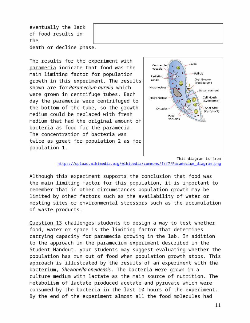
The results for the experiment with paramecia indicate that food was the main limiting factor for population growth in this experiment. The results shown are for Paramecium aurelia which were grown in centrifuge tubes. Each day the paramecia were centrifuged to the bottom of the tube, so the growth medium could be replaced with fresh medium that had the original amount of bacteria as food for the paramecia. The concentration of bacteria was twice as great for population 2 as for population 1.

This diagram is from https://upload.wikimedia.org/wikipedia/commons/f/f7/Paramecium_diagram.png

Although this experiment supports the conclusion that food was the main limiting factor for this population, it is important to remember that in other circumstances population growth may be limited by other factors such as the availability of water or nesting sites or environmental stressors such as the accumulation of waste products.

Question 13 challenges students to design a way to test whether food, water or space is the limiting factor that determines carrying capacity for paramecia growing in the lab. In addition to the approach in the paramecium experiment described in the Student Handout, your students may suggest evaluating whether the population has run out of food when population growth stops. This approach is illustrated by the results of an experiment with the bacterium, Shewanella oneidensis. The bacteria were grown in a culture medium with lactate as the main source of nutrition. The metabolism of lactate produced acetate and pyruvate which were consumed by the bacteria in the last 10 hours of the experiment. By the end of the experiment almost all the food molecules had been consumed, which probably was the reason why population growth was ending. If you want to introduce this example, you could use the following.

7

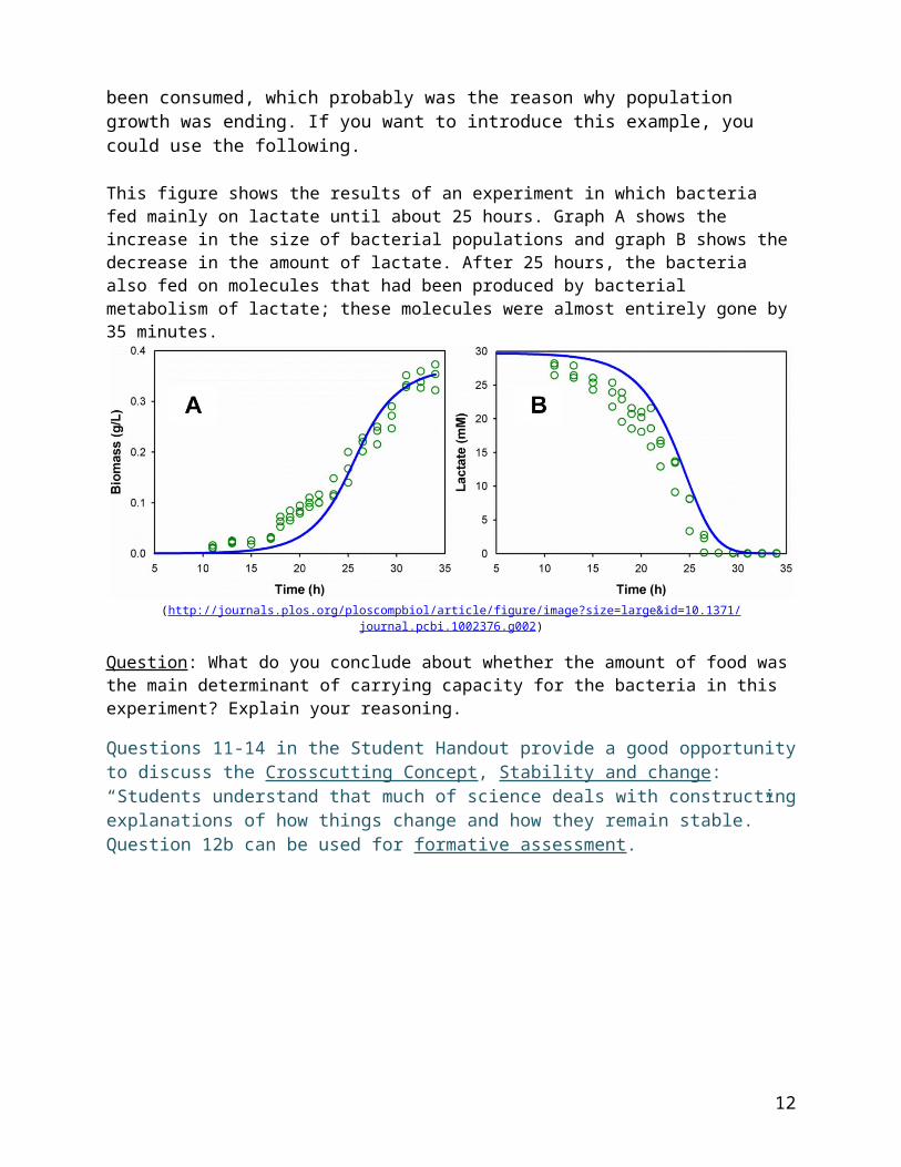
This figure shows the results of an experiment in which bacteria fed mainly on lactate until about 25 hours. Graph A shows the increase in the size of bacterial populations and graph B shows the decrease in the amount of lactate. After 25 hours, the bacteria also fed on molecules that had been produced by bacterial metabolism of lactate; these molecules were almost entirely gone by 35 minutes.

(http://journals.plos.org/ploscompbiol/article/figure/image?size=large&id=10.1371/journal.pcbi.1002376.g002)

Question: What do you conclude about whether the amount of food was the main determinant of carrying capacity for the bacteria in this experiment? Explain your reasoning.

Questions 11-14 in the Student Handout provide a good opportunity to discuss the Crosscutting Concept, Stability and change: “Students understand that much of science deals with constructing explanations of how things change and how they remain stable.” Question 12b can be used for formative assessment.

8

IV. Using the Exponential and Logistic Population Growth Models to Understand Recovery of Endangered SpeciesA model is a representation of reality that highlights certain key aspects of a phenomenon and thus helps us to better understand and visualize the phenomenon. However, as discussed in this section, all models involve assumptions and simplifications of complex real-world phenomena, so there may be discrepancies between a model’s predictions and phenomena observed in the real world. Many students tend to think of a model as a physical object and may not understand how a graph or equation can be a model. It may be helpful to introduce the idea of a conceptual model. As noted in A Framework for K-12 Science Education, “Conceptual models allow scientists… to better visualize and understand a phenomenon under investigation… Although they do not correspond exactly to the more complicated entity being modeled, they do bring certain features into focus while minimizing or obscuring others. Because all models contain approximations and assumptions that limit the range of validity of their application and the precision of their predictive power, it is important to recognize their limitations.” 8

To help your students understand conceptual models, you can give examples of conceptual models that students may have used, e.g. a map, a diagram of a football play, a concept map, or an outline for an essay they plan to write. Then, you can ask them about the strengths and weaknesses of these conceptual models and try to elicit student ideas that will lead to the Crosscutting Concept, “Models can be used to predict the behavior of a system, but these

8 Quotation from A Framework for K-12 Science Education: Practices, Crosscutting Concepts, and Core Ideas (available at http://www.nap.edu/catalog.php?record_id=13165).

Notes for Mathematical Equations on page 5 of the Student Handout

The only difference between the equations for exponential and logistic population growth is the term (K – N) / K in the logistic population growth equation. This term represents the reduction in growth rate caused by the effects of density-dependent factors. At low population size (N), this term is close to 1, so logistic population growth is quite similar to exponential population growth. As population size increases and approaches the carrying capacity (K) of the environment, this term approaches zero, reflecting the effects of increasing competition for limited resources. The most rapid increase in population size is observed when N = 0.5 K; population size increases more slowly at lower levels of N (because there are relatively few individuals reproducing) and at higher levels of N (due to the effects of competition for scarce resources, increased risk of infection, etc.). This suggests that, for maximal sustainable harvest, it may be best to maintain a population at half the carrying capacity.

The mathematical equations and the graphs are two different types of representation of the exponential and logistic population growth models. The equations for exponential and logistic population growth have the advantage of helping us to understand the reasons for the different rates of increase at different population sizes. Also, these equations facilitate quantitative predictions concerning changes in population size. In contrast, the graphs have the advantage of giving a better intuitive feel for the trends in population size. Thus, both types of representation of these population growth models are useful for different purposes.

Question 17 can be used for formative assessment.

9

predictions have limited precision and reliability due to the assumptions and approximations inherent in models”.

Question 15/18 reinforces student understanding of the difference between linear and exponential population growth.

As discussed in question 16/19, additional populations in different locations help to reduce the risk of extinction by providing protection against a possible catastrophe in one location (e.g. due to a hurricane or infectious disease epidemic) and by providing additional habitat to support growth of whooping crane populations. A second population of migrating whooping cranes has been established through a captive breeding program and careful training of the young whooping cranes to survive in the wild (https://www.youtube.com/watch?v=Ye4Swf3-yDM). Young whooping cranes bond with the first moving object they see; to ensure that the captive-bred birds will subsequently mate with other whooping cranes, the people who raise them wear crane costumes (https://www.savingcranes.org/wp-content/uploads/2015/01/a_journey_through_time.pdf).9 For additional information about whooping cranes and the conservation efforts, see https://www.fws.gov/northflorida/whoopingcrane/whoopingcrane-fact-2001.htm and http://www.learner.org/jnorth/search/Crane.html.

Question 17/20 could easily lead to a more general discussion of endangered species and the Endangered Species Act. Two useful general sources on endangered species are https://www.fs.fed.us/rm/pubs_journals/2016/rmrs_2016_evans_d001.pdf and https://www.nytimes.com/2018/03/13/magazine/should-some-species-be-allowed-to-die-out.html.

Questions 15-17/18-20 provide another good opportunity for peer discussion and feedback.

V. Exponential and Logistic Population Growth Models vs. Complex RealityThis section helps students to understand the limitations of the exponential and logistic population growth models. In question 18/21, students contrast the roughly exponential growth for the whooping crane population in recent decades vs. the longer-term trends in total number of whooping cranes which do not follow either the exponential or logistic population growth models. This provides the opportunity to discuss the Crosscutting Concept, Scale, Proportion and Quantity: “Patterns observable at one scale may not be observable or exist at other scales.” You might want to mention that when scale changes by one or more orders of magnitude, there are even more dramatic changes in the significance of phenomena.

Next, students analyze trophic effects in a marine ecosystem. They learn how changes in the population size of a predator can have important effects on the population size of other species in a food web.10 Sea otters were rare in the first half of the twentieth century due to human hunting.

9 Funding for this captive breeding program for whooping cranes was eliminated in 2017 (http://blog.nwf.org/2018/01/a-wild-year-for-the-whooping-crane/).10 Another example of trophic effects on changes in population size is discussed in our activity “Food Webs, Energy Flow, Carbon Cycle and Trophic Pyramids” (http://serendipstudio.org/exchange/bioactivities/foodweb). Analyses of the effects of reintroducing wolves in an ecosystem in Canada have shown that wolves increased mortality and decreased population size of a dominant herbivore which resulted in increased net growth of willows which in turn provided more nesting sites and cover for songbirds in stream and river valleys (Hebblewhite et al., Ecology 86:2135, 2005). This example illustrates that the availability of nesting sites and places to avoid predation can influence carrying capacity.

10

In the mid-twentieth century, legal protections for sea otters allowed them to become abundant, with major effects on populations of sea urchins and kelp (http://urchinsandkelpforests.blogspot.com/). This example illustrates how understanding the interactions between the species in an ecological community can be important for understanding changes in population size for the species in that community. If you either prefer not to or can’t show your students the video at https://ww2.kqed.org/quest/2014/02/25/balancing-act-otters-urchins-and-kelp/, you can substitute the following alternative wording which does not require the video.

19/22a. As a result of human hunting, sea otters were rare at the beginning of the twentieth century. Then, hunting was restricted, and sea otters became abundant. When the number of sea otters increased, the sea urchin population size _________________. Explain your reasoning.

(increased / decreased)

19/22b. As a result of the change in sea urchin population size, the kelp population size __________________. Explain your reasoning. (increased / decreased)

Question 20/23 focuses student attention on the progression from the exponential population growth model (which includes increases in population size as a result of reproduction) to the logistic population growth model (which adds the effects of competition for limited resources) to a more complete description of the causes of changes in size for real-world populations (which adds the effects of changes in the environment). This provides a good opportunity to discuss the Crosscutting Concept of Systems and System Models which states that models can be used “to predict the behavior of a system, [but] these predictions have limited precision and reliability due to the assumptions and approximations inherent in the models”. Because environments do not have the unlimited resources assumed in the exponential growth model, exponential growth is only observed during the early stages of population growth, e.g. when a species moves into a new environment or is recovering from a catastrophes such as excessive hunting by humans. Similarly, logistic population growth of natural populations often does not culminate in stable population size at carrying capacity, as predicted by the logistic population growth model. For many natural populations, changes in the environment cause variation in carrying capacity which results in variation in population size.

The reindeer example illustrates that, when a population size exceeds carrying capacity, the environment may be degraded (e.g. due to overgrazing); this results in reduced carrying capacity which can cause a crash in population size. The large population of reindeer in the late 1930s (estimated to be approximately three times the carrying capacity of the island) nearly eliminated the lichens which were a critical winter food for the reindeer; the slow-growing lichens had not significantly regenerated when studied ~1950.11 Discussion of this example may lead to interest in whether human population growth may degrade the environment, reduce the carrying capacity

11 Severe winter weather appears to have contributed to the rapid population decline around 1940, but population size continued to decline even when the winter weather ameliorated (Scheffer, The Scientific Monthly 73: 356, 1951). In recent years, there have been roughly 400 reindeer on this island. The lichen have not regrown, but the reindeer have switched to grasses and roots for their winter food. Hunting by humans has kept the reindeer numbers within the new carrying capacity. This recent change in the winter feeding behavior of these reindeer has increased the carrying capacity from the low point ~1950 (https://www.alaskapublic.org/2017/01/23/st-pauls-reindeer-thrive-without-essential-lichen/ ) . Reindeer introduced on a nearby island showed much less dramatic increases and decreases in population size; the reasons for the differences between the islands are unknown. General information about reindeer is available at https://www.uaf.edu/files/snras/MP_04_07.pdf.

11

of the earth, and possibly lead to a population crash; the next section of the Student Handout provides some relevant information. Question 23/26 reinforces student understanding that the logistic population growth model is only valid if the two simplifying assumptions are true (see the top of page 7/8 in the Student Handout).

To illustrate how research methods can influence the conclusions reached, you could add the following question.

24/27. Suppose that the reindeer researchers had stopped collecting data in 1937. What would they have concluded about reindeer population growth? What would they have missed?

This example illustrates how conclusions can vary, depending on the specific data collected. Thus, reliable conclusions should be based on the results of multiple different studies, and we should be skeptical about conclusions based on a single study. In the discussion of this optional question, I recommend that you reinforce these general methodological points. This addition to the Student Handout would also provide the opportunity to discuss the Crosscutting Concept, Scale, Proportion and Quantity: “Patterns observable at one scale may not be observable or exist at other scales.”

If your students would benefit from another example that logistic population growth is not observed unless carrying capacity is constant, you could use the following question before the reindeer example.

21a/24a. This graph shows seasonal changes in population size for a population of rabbits that lived in Ohio. How did population size change from October to January each year?

21b/24b. What caused the decrease in population size between October and January? Was carrying capacity constant?

This optional question would help students to understand that both abiotic and biotic factors influence population dynamics. Seasonal changes in weather are density-independent factors12 that limit the growth of many populations of short-lived plants and animals. During the growing season, population size may increase exponentially and then, during the cold and/or dry season, the carrying capacity of the environment drops dramatically and population size decreases correspondingly. As you discuss this question, you can alert your students to an important methodological issue. Ask them what would have happened if the researchers only measured population size once a year at the same time each year. What important effect would the researchers have missed?

If your students would benefit from another example where population size exceeded carrying capacity because rates of reproduction and mortality did not respond quickly enough as

12 Density-independent factors include freezing weather, tornadoes, floods and fires, each of which can drastically reduce population size, independent of initial population density. Neither the exponential population growth model nor the logistic population growth model takes account of the effects of density-independent factors on population size.

12

population size approaches carrying capacity, you could use the following before the reindeer example.13

The line in this figure shows logistic population growth. The dots show the trends in population size for a laboratory population of Daphnia (water fleas) that had a constant supply of food.

On days 50-60, food was scarce, but Daphnia continued to reproduce, using their fat stores as a substitute for food. After about day 70, food was so scarce that many Daphnia starved to death and population size was reduced to the carrying capacity. (http://www.bio.miami.edu/dana/pix/logisticpopns.gif)

21a/24a. Circle the part of the graph where population size exceeds the carrying capacity.

21a/24b. How did population size increase above the carrying capacity? How did the Daphnia continue to reproduce even though food was scarce?

Question 24/27 in the Student Handout engages students in synthesizing the models Crosscutting Concept, the Scientific Practices of using models and constructing explanations, and the Disciplinary Core Idea LS2.A. If your students find this question too challenging, you could:

help your students review key points from pages 1-7/1-8 of the Student Handout have them discuss the question first in pairs or small groups and then write their

individual answers.This question can be used for formative assessment. This question also provides a good opportunity for class discussion with peer feedback.

V. Human Population GrowthThis section focuses on total world population, rather than the size of local populations. One reason for this approach is that migration and world trade result in many interconnections between local human populations. Also, total world population is one factor of concern in environmental problems such as endangered species and global warming.

You may want to begin this section with a discussion of students’ prior understanding of world population growth. Also you may want to show your students the animation at https://www.youtube.com/watch?v=PUwmA3Q0_OE (~6.5 minutes long) to help them understand the slow pace of population growth in the early millennia of human existence and the much more rapid pace lately. The last part of this animation has a brief introduction to projections of future population growth, including the importance of decreased birth rates and reasons for uncertainty in the projections. This part of the animation provides the opportunity to ask your students why 2 babies per woman will eventually result in stable population size. (Actually, to take account of mortality before reproductive age, the number should be 2.1 babies per woman on average.) To give your students a feel for the rate of current population growth, you may want to use the “worldometer” at http://www.worldometers.info/world-population/.

13 It may be helpful to know that, in the Daphnia experiment, the researchers restored the original density of algae as food for the Daphnia each day and they moved the Daphnia population to fresh water every third day.When population growth rate adjusts slowly to changes in population size, then population size may repeatedly overshoot and undershoot the carrying capacity, resulting in cyclic changes in population size (http://www.cfr.washington.edu/classes.esrm.450/Lecture13/Cycles.pdf ) .

13

Question 25/28 reinforces student understanding of exponential population growth. However, you should be aware that, during much of the twentieth century, world population increased faster than exponential growth. Exponential population growth would have a constant percent annual growth rate, but this rate increased during the early twentieth century (see figure below). Advances in public health, standard of living and healthcare resulted in decreased mortality and increased population growth. Fertility declines followed with a lag of roughly half a century, so the population growth rate declined in the second half of the twentieth century. For additional information about past trends in world population growth, projections for future population growth, and factors that have influenced and will influence these trends, see https://esa.un.org/unpd/wpp/publications/Files/WPP2017_KeyFindings.pdf and https://www.prb.org/humanpopulation/.

(https://ourworldindata.org/world-population-growth)

Human behavior has had and will have profound effects on the carrying capacity of the Earth for humans. Humans have increased the amount of food that can be produced by developing better breeds of plants and animals, using fertilizers and irrigation, etc.; increased agricultural productivity has increased the number of people that can be fed substantially beyond previous pessimistic predictions by Malthus and Ehrlich (https://www.ncbi.nlm.nih.gov/pmc/articles/PMC1280423/). On the other hand, increasing levels of consumption will reduce the number of people that the earth can sustain. The following sources discuss the wide range of estimates of the Earth’s carrying capacity and the multiple factors that have influenced and will influence the Earth’s carrying capacity:

https://na.unep.net/geas/getUNEPPageWithArticleIDScript.php?article_id=88 http://agrpartners.com/wp-content/uploads/2013/09/AGR-Thought-Piece-Carrying-

Capacity1.pdf

14

https://www.livescience.com/16493-people-planet-Earth-support.html (which has a brief video outlining some of the major issues).

The table below shows the data for the comparisons in question 27/30 between per capita consumption in the US vs. the world average. These data are “food availability” for 2013, which does not take into account food that is wasted or not eaten by consumers. Nevertheless, it is clear that US consumption levels are well in excess of the optimum level for human health.

Average Consumption per Person per DayCalories Grams of Meat Grams of Protein

US ~3700 ~115 ~110World ~2900 ~43 ~80

(Sources: https://ourworldindata.org/food-per-person; https://ourworldindata.org/meat-and-seafood-production-consumption)

The Optional Challenge Question introduces students to limited groundwater as one factor that may limit the Earth’s carrying capacity for humans. The sources for the first paragraph of this question include:

https://www.linkedin.com/pulse/new-satellite-measurements-show-world-aquifers-main- belen-cavanillas

https://www.nasa.gov/jpl/grace/study-third-of-big-groundwater-basins-in-distress/ https://water.usgs.gov/edu/gwdepletion.html .

If your students use the recommended sources to answer the Challenge Question, I recommend that you have them read the sources first and then set the sources aside while they draft their answers. That way, the students will write their answers entirely in their own words, based on their understanding of the material. After drafting their answers, students can return to the sources to check and correct specific information in their answers. The first recommended source has a video at the end which you probably won’t want to use; you might prefer “10 Ways Farmers Are Saving Water” (https://cuesa.org/article/10-ways-farmers-are-saving-water). For more information about the large amount of water needed to grow meat, see “The Hidden Water Resource Use Behind Meat and Dairy” (http://waterfootprint.org/media/downloads/Hoekstra-2012-Water-Meat-Dairy_1.pdf).

You will probably want to mention that the Earth’s carrying capacity for humans will be limited not only by consumption of resources, but also by production of waste products. To introduce one example, I recommend the analysis and discussion activity “Food, the Carbon Cycle, and Global Warming – How can we feed a growing world population without increasing global warming?” (http://serendipstudio.org/exchange/bioactivities/global-warming). In the first section of this analysis and discussion activity, students analyze information about global warming and greenhouse gases such as carbon dioxide. Students learn that correlation does not necessarily imply causation and analyze the types of evidence that establish causal relationships. In the next two sections, students analyze carbon cycles, the effects of food production on greenhouse gas emissions, and the reasons why more greenhouse gases are emitted during the production of meat compared to plant-based foods. The last section engages students in proposing and researching ways to feed the world’s growing population without increasing global warming. 

Additional Resources A possible alternative activity (e.g. for middle school students) is “Some Similarities between

the Spread of Infectious Disease and Population Growth”. This hands-on activity introduces

15

students to some features of exponential and logistic population growth. First, students analyze a hypothetical example of exponential growth in the number of infected individuals. Then, a class simulation of the spread of an infectious disease shows a trend that approximates logistic growth. Next, students analyze examples of exponential and logistic population growth and learn about the biological processes that result in exponential or logistic population growth. Finally, students analyze how changes in the biotic or abiotic environment can affect population size; these examples illustrate the limitations of the exponential and logistic population growth models. This activity is aligned with the Next Generation Science Standards. (http://serendipstudio.org/sci_edu/waldron/#infectious)

“Population Dynamics” is a good online simulation that will reinforce student understanding of basic concepts and the mathematics of population growth (http://ats.doit.wisc.edu/biology/ec/pd/pd.htm).

“Population Ecology” is a useful curriculum that reviews population ecology and relates population ecology to analysis of invasive species (http://landbasedlearning.org/slews-curriculum-es). This site also provides curriculum units on other aspects of ecology.

Students can learn about the effects of species interactions in ecological communities by studying invasive species – e.g. “Race to Displace: a Game to Model the Effects of Invasive Species on Plant Communities” (http://schoolpartnership.wustl.edu/wp-content/uploads/2013/02/RaceToDisplace-ABT201375310-Inquiry-Investigations-Hopwood.pdf) or “Effects of Zebra Mussels on the Hudson River” (http://www.caryinstitute.org/educators/teaching-materials/changing-hudson-project and see update at http://www.caryinstitute.org/newsroom/zebra-mussels-losing-their-grip-hudson-river-ecosystem-rebounding) or sections of “Population Dynamics” described above.

“Population Dynamics: Mystery of the Missing Housefly” provides an entertaining and informative web-based activity that introduces students to many of the same concepts covered in this activity (http://mathbench.umd.edu/modules/popn-dynamics_housefly/page01.htm).

Sources for Figures and Data in Table Picture of Whooping Crane – http://www.audubon.org/field-guide/bird/whooping-crane Graph and Table of Trends in Whooping Crane Population Size – adapted from

https://www.sciencedirect.com/science/article/pii/S0006320713000980, Figure 1 and Table 1, plus https://www.fws.gov/uploadedFiles/Region_2/NWRS/Zone_1/Aransas-Matagorda_Island_Complex/Aransas/Sections/What_We_Do/Science/Whooping_Crane_Updates_2013/WHCR_Update_Winter_2016-2017.pdf

Food Poisoning Illustration – based on https://static.shakethatweight.co.uk/uploads/filter-porridge-1.svg, https://i.pinimg.com/originals/d5/7c/f9/d57cf9fa76b9a87c5a9157cbc8c3a6a9.jpg, and https://www.jagranjosh.com/imported/images/E/Articles/Diseases-caused-by-food-poisoning.png

Graph of Logistic Population Growth for Bacteria – adapted from https://ars.els-cdn.com/content/image/1-s2.0-S002364381630768X-gr1.jpg

Exponential and Logistic Population Growth – adapted from https://swh-826d.kxcdn.com/wp-content/uploads/2011/12/exponential-vs-logistic-growt.jpg

Graph of Logistic Population Growth for Paramecia – based on data from “The Struggle for Existence”, by G. F. Gause, 1934

Annual Variation in Rabbit Population Size – adapted from https://populationeducation.org/sites/default/files/pop_ecology_files.pdf

16

Trends in Size of Reindeer Population – http://go.hrw.com/resources/go_sc/bpe/HE0PE332.PDF

World Population Growth (prepared by Allianz) – adapted from http://populationoverview.weebly.com/uploads/6/0/1/3/60138411/253768413.jpg?726

17