population admixture - data.broadinstitute.org filealkes price harvard school of public health...
TRANSCRIPT
Alkes Price
Harvard School of Public Health
February 19 & February 21, 2019
EPI 511, Advanced Population and Medical Genetics
Week 4:
• Population admixture

Outline
1. Admixture leads to variation in genome-wide ancestry
2. Admixture creates mosaic chromosomes
3. Local ancestry inference
4. Evaluating local ancestry inference algorithms

Outline
1. Admixture leads to variation in genome-wide ancestry
2. Admixture creates mosaic chromosomes
3. Local ancestry inference
4. Evaluating local ancestry inference algorithms


Hellenthal et al. 2014 Science
What is an admixed population?
An admixed population is a population with recent
ancestry from two or more continents
(e.g. within the past 1,000 years).

What is an admixed population?
An admixed population is a population with recent
ancestry from two or more continents
(e.g. within the past 1,000 years).
Note: the word “admixture” is also sometimes used to
refer to more ancient admixture events. (e.g. Patterson et al. 2012 Genetics, Hellenthal et al. 2014 Science)

Population structure vs. Population admixture:
What’s the difference?
Population structure: [Week 3]
• Genetic differences due to geographic ancestry.
• Use genome-wide data to infer genome-wide ancestry.
Population admixture: [Week 4]
• Mixed ancestry from multiple continental populations.
• e.g. African Americans, Latino Americans.
• Infer local ancestry at each location in the genome.
Population admixture implies population structure.
Population structure does not imply population admixture.
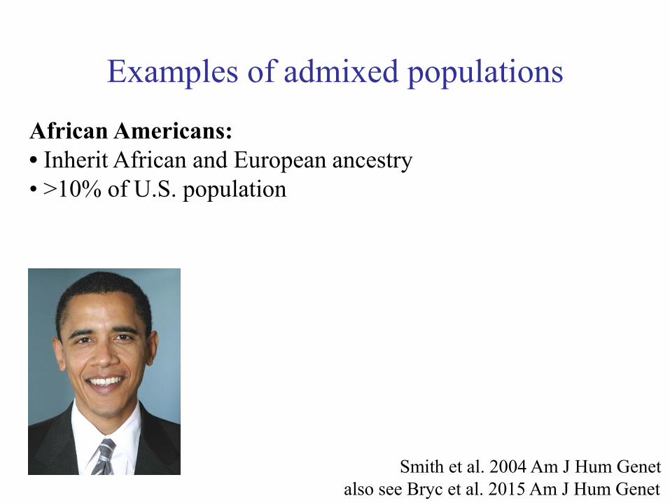
Examples of admixed populations
African Americans:
• Inherit African and European ancestry
• >10% of U.S. population
Smith et al. 2004 Am J Hum Genet
also see Bryc et al. 2015 Am J Hum Genet

Examples of admixed populations
Hispanic/Latino Americans:
• Inherit European and Native American
or European, Native American and African ancestry
• e.g. Mexican Americans, Puerto Ricans, etc.
• >15% of U.S. population
Bryc, Velez et al. 2010 PNAS
also see Bryc et al. 2015 Am J Hum Genet

Examples of admixed populations
Latinos outside the U.S.:
• Inherit European and Native American
or European, Native American and African ancestry
• hundreds of millions of people throughout Latin America
Bryc, Velez et al. 2010 PNAS
also see Bryc et al. 2015 Am J Hum Genet

An aside: Characteristics of African,
European and Native American populations
African populations:
• High within-population diversity, low LD (no bottleneck).
• Low genetic distance (FST) between West African populations
European populations:
• Lower within-population diversity, higher LD (bottleneck).
• Low genetic distance (FST) between European populations
Native American populations:
• Lowest within-population diversity, highest LD due to
multiple population bottlenecks.
• Very high FST between Native American populations
Cavalli-Sforza et al. 1994 The History and Geography of Human Genes
Reich et al. 2012 Nature

Other examples of admixed populations
Native Hawaiians (Polynesian, European, East Asian ancestry)
Uyghurs (East Asian and European-related ancestry)
A population that self-identifies and is described in the
the academic literature as “South African Coloured” (San African, Bantu African, European, S Asian, SE Asian ancestry)
Haiman et al. 2003 Hum Mol Genet,
Haiman et al. 2007 Nat Genet
Xu, Huang et al. 2008 Am J Hum Genet,
Xu & Jin 2008 Am J Hum Genet
de Wit et al. 2010 Hum Genet, Patterson et al. 2010 Hum Mol Genet,
Tishkoff et al. 2009 Science, Chimusa et al. 2013 Hum Mol Genet

Inferring genome-wide ancestry proportions
Apply the usual clustering programs, allowing fractional ancestry
(see Week 3 slides):
• STRUCTURE (Pritchard et al. 2000 Genetics, Falush et al. 2003 Genetics)
• FRAPPE (Tang et al. 2005 Genet Epidemiol, Li et al. 2008 Science)
• ADMIXTURE (Alexander et al. 2009 Genome Res)
Or, apply principal components analysis
(see Week 3 slides):
• PCA (Price et al. 2006 Nat Genet, Patterson et al. 2006 PLoS Genet)

Admixture leads to variation in genome-wide ancestry
AA: 21% ± 14%
European ancestry
YRI
CHB+JPT
CEU
African Americans
Price, Patterson et al. 2008 PLoS Genet
also see Smith et al. 2004 Am J Hum Genet; Bryc et al. 2015 Am J Hum Genet
(from Week 3)
PC1
PC2

Admixture proportion varies across individuals,
but also varies with U.S. geographic location
Kittles et al. 2007 CJHP
also see Bryc et al. 2015 Am J Hum Genet, Baharian et al. 2016 PLoS Genet
% European ancestry in African American populations
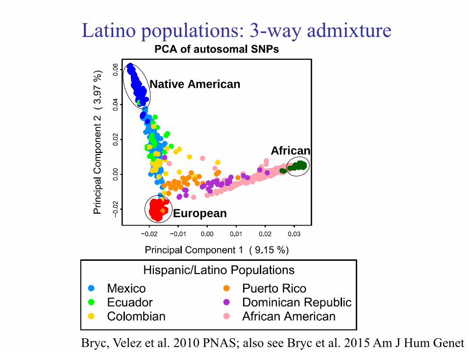
Latino populations: 3-way admixture
Bryc, Velez et al. 2010 PNAS; also see Bryc et al. 2015 Am J Hum Genet
European
Native American
African

Latino populations: 3-way admixture
Price et al. 2007 Am J Hum Genet; also see Bryc, Velez et al. 2010 PNAS;
Moreno-Estrada et al. 2014 Science; Bryc et al. 2015 Am J Hum Genet
Mexican Americans
50% European, 45% Native American, 5% African on average,
with substantial variation among individuals.
Puerto Ricans
60% European, 20% Native American, 20% African on average,
with substantial variation among individuals.
Brazilians and Colombians
70% European, 20% Native American, 10% African on average,
with substantial variation among individuals. [For populations sampled. Values may not apply to all populations.]

Different Native American ancestral populations
for Latino populations in different regions
Wang et al. 2008 PLoS Genet
also see Price et al. 2007 Am J Hum Genet

CEU northern European USA 180
CHB Chinese China 90
JPT Japanese Japan 90
YRI Yoruba Nigeria 180
TSI Tuscan Italy 90
CHD Chinese USA 100
LWK Luhya Kenya 90
MKK Maasai Kenya 180
ASW African-American USA 90
MXL Mexican-American USA 90
GIH Gujarati-American USA 90
Which HapMap3 populations are admixed?

PCA of all HapMap3 populations
International HapMap3 Consortium 2010 Nature (see Supp Figures)

These populations are “homogeneous”
in their continental ancestry
International HapMap3 Consortium 2010 Nature (see Supp Figures)
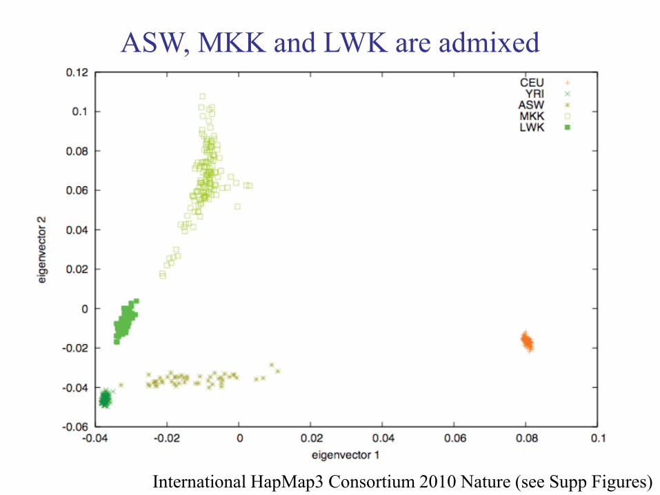
ASW, MKK and LWK are admixed
International HapMap3 Consortium 2010 Nature (see Supp Figures)

ASW, MKK and LWK are admixed
International HapMap3 Consortium 2010 Nature (see Supp Figures)
Bantu expansion
(2000 BC – 1000 AD)
Arab migrations
(500 – 1500 AD)
(Cavalli-Sforza et al. 1994,
The History and Geography
Of Human Genes)
X Ancestral East African population

STRUCTURE results on African populations
= West African/Bantu
= East African
= Khoisan
= Pygmy
= European/Middle Eastern
Tishkoff et al. 2009 Science; also see Gurdasani et al. 2015 Nature
K=14:
(from Week 3)

MXL (Mexican Americans) are admixed
International HapMap3 Consortium 2010 Nature (see Supp Figures)

Are GIH (Gujarati Americans) admixed?
International HapMap3 Consortium 2010 Nature (see Supp Figures)
also see Reich et al. 2009 Nature, Nakatsuka et al. 2017 Nat Genet

Are GIH (Gujarati Americans) admixed?
International HapMap3 Consortium 2010 Nature (see Supp Figures)
also see Reich et al. 2009 Nature, Nakatsuka et al. 2017 Nat Genet

Are GIH (Gujarati Americans) admixed?
International HapMap3 Consortium 2010 Nature (see Supp Figures)
also see Reich et al. 2009 Nature, Nakatsuka et al. 2017 Nat Genet

Which HGDP populations are admixed?
Li et al. 2008 Science
938 HGDP individuals
Illumina 650K chip (from Week 3)

Which HGDP populations are admixed?
Li et al. 2008 Science
admixture in
Middle East / North Africa?
Recent? Or not? (Price, Tandon et al. 2009 PLoS Genet)

European Americans: 3-way admixture!
Bryc et al. 2015 Am J Hum Genet
European Americans
>99% European,
0.2% Native American,
0.2% African on average
with substantial variation
among individuals.

Trees can also describe population structure
Unrooted tree Rooted tree Jakobsson et al. 2008 Nature Li et al. 2008 Science
(from Week 3)
also see Cavalli-Sforza et al. 2003 Nat Genet

Trees cannot model recent admixture
root
YRI CEU
root
YRI CEU ASW ASW
WRONG. WRONG.
Outline
1. Admixture leads to variation in genome-wide ancestry
2. Admixture creates mosaic chromosomes
3. Local ancestry inference
4. Evaluating local ancestry inference algorithms

Admixture creates mosaic chromosomes
Population 1 Population 2
1 generation later

Population 1 Population 2
2 generations later
Admixture creates mosaic chromosomes

Population 1 Population 2
several generations later
Admixture creates mosaic chromosomes
Local ancestry = 0, 1 or 2
copies from population 1

Population 1 Population 2
Admixture creates mosaic chromosomes
several generations later
Local ancestry = 0, 1 or 2
copies from population 1
Average segment length (in Morgans) ~ 1/g
where g = average #generations since admixture
g ≈ 6 for African Americans, g ≈ 10 for Latino populations
Smith et al. 2004 Am J Hum Genet, Price et al. 2007 Am J Hum Genet

Mosaic chromosomes create admixture-LD
Toy example: Admixed population with 50% POP1, 50% POP2
SNP1 = A/C SNP, A allele has frequency 0.10 in POP1, 0.90 in POP2
SNP2 = A/C SNP, A allele has frequency 0.10 in POP1, 0.90 in POP2
SNP1 and SNP2 are unlinked in POP1, unlinked in POP2.
SNP1 and SNP2 are 200kb apart: (nearly) always same local ancestry.
P(SNP1=A, SNP2=A) = 50%·0.10·0.10 + 50%·0.90·0.90 = 0.41
POP1 POP2

Mosaic chromosomes create admixture-LD
Toy example: Admixed population with 50% POP1, 50% POP2
SNP1 = A/C SNP, A allele has frequency 0.10 in POP1, 0.90 in POP2
SNP2 = A/C SNP, A allele has frequency 0.10 in POP1, 0.90 in POP2
SNP1 and SNP2 are unlinked in POP1, unlinked in POP2.
SNP1 and SNP2 are 200kb apart: (nearly) always same local ancestry.
P(SNP1=A, SNP2=A) = 50%·0.10·0.10 + 50%·0.90·0.90 = 0.41
P(SNP1=A, SNP2=C) = 50%·0.10·0.90 + 50%·0.90·0.10 = 0.09
P(SNP1=C, SNP2=A) = 50%·0.90·0.10 + 50%·0.10·0.90 = 0.09
P(SNP1=C, SNP2=C) = 50%·0.90·0.90 + 50%·0.10·0.10 = 0.41
SNP1 and SNP2 are in admixture-LD in the admixed population!
slide repeated in Week 6

Admixture-LD depends on allele frequency differences
Toy example: Admixed population with 50% POP1, 50% POP2
SNP1 = A/C SNP, A allele has frequency 0.10 in POP1, 0.10 in POP2
SNP2 = A/C SNP, A allele has frequency 0.10 in POP1, 0.90 in POP2
SNP1 and SNP2 are unlinked in POP1, unlinked in POP2.
SNP1 and SNP2 are 200kb apart: (nearly) always same local ancestry.
P(SNP1=A, SNP2=A) = 50%·0.10·0.10 + 50%·0.10·0.90 = 0.05
P(SNP1=A, SNP2=C) = 50%·0.10·0.90 + 50%·0.10·0.10 = 0.05
P(SNP1=C, SNP2=A) = 50%·0.90·0.10 + 50%·0.90·0.90 = 0.45
P(SNP1=C, SNP2=C) = 50%·0.90·0.90 + 50%·0.90·0.10 = 0.45
No allele frequency difference in SNP1 => no admixture-LD.

Mosaic chromosomes create admixture-LD
Real example of admixture-LD:
rs164781: 0.42 in CEU, 0.88 in YRI (HapMap3)
rs10495758: 0.88 in CEU, 0.32 in YRI (HapMap3)
These SNPs are located roughly 3Mb apart.
r2 between rs164781 and rs10495758:
0.01 in CEU, 0.01 in YRI, 0.28 in ASW (HapMap3)
rs164781 and rs10495758 are in admixture-LD in ASW!
International HapMap3 Consortium 2010 Nature
SNPs chosen from Tandon et al. 2011 Genet Epidemiol
slide repeated in Week 4 bonus slides
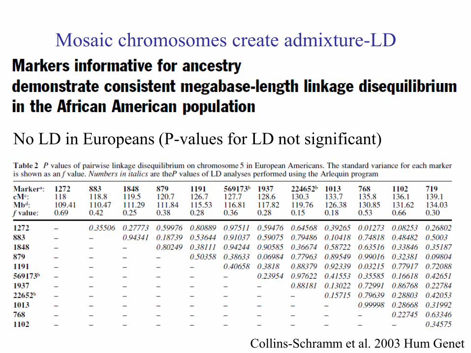
Mosaic chromosomes create admixture-LD
Collins-Schramm et al. 2003 Hum Genet
No LD in Europeans (P-values for LD not significant)

Mosaic chromosomes create admixture-LD
Collins-Schramm et al. 2003 Hum Genet
Admixture-LD in African Americans (significant P-values)

Local ancestry = 0, 1 or 2
copies from population 1
at a specific locus
Local ancestry vs. Genome-wide ancestry
Local
ancestry
Genome-wide
ancestry
Genome-wide ancestry
(e.g. 20% European)

Outline
1. Admixture leads to variation in genome-wide ancestry
2. Admixture creates mosaic chromosomes
3. Local ancestry inference
4. Evaluating local ancestry inference algorithms

Ancestry-informative marker (AIM) panels for
local ancestry inference in African Americans
The most
informative
~1% of
SNPs
provide
powerful
information
about
ancestry
0%
20%
40%
60%
80%
100%
0% 20% 40% 60% 80% 100%
European American Frequency
We
st
Afr
ica
n F
req
ue
nc
y
Smith et al. 2004
• Choose 1,500-3,000 SNPs with large Δ(EUR,AFR)
(unlinked, i.e. not in LD, in ancestral populations)
Smith et al. 2004 Am J Hum Genet
Tian et al. 2006 Am J Hum Genet (slide from David Reich)
The most informative SNPs
provide powerful information
about local ancestry
“African-American
admixture map”

Ancestry-informative marker (AIM) panels for
local ancestry inference in Latino populations
Price et al. 2007 Am J Hum Genet
Mao et al. 2007 Am J Hum Genet
Tian et al. 2007 Am J Hum Genet
The most informative SNPs
provide powerful information
about local ancestry
“Latino admixture map”
• Choose 1,500-3,000 SNPs with large Δ(EUR,NA)
(unlinked, i.e. not in LD, in ancestral populations)

Local ancestry = 0, 1 or 2
copies from population 1
at a specific locus
Local ancestry vs. Genome-wide ancestry
Local
ancestry
Genome-wide
ancestry
Genome-wide ancestry
(e.g. 20% European)
25-50 AIMs
1,500-3,000 AIMs

Inferring local ancestry using AIM panels
SNP chr position Eur freq Afr freq
rs2814778 1 159,174,683 0% 100%
1 SNP with Δ=100%: perfect information about local ancestry
Duffy blood group locus
see Hamblin et al. 2000 Am J Hum Genet, Hamblin et al. 2002 Am J Hum Genet
slide repeated in Week 6 bonus slides, slide repeated in Week 7

Inferring local ancestry using AIM panels
SNP chr position Eur freq Afr freq
rs1962508
rs2806424
rs1780349
1
1
1
158,677,077
159,423,117
161,340963
4%
84%
44%
74%
26%
99%
Several SNPs with Δ=60-80%: ???

Inferring local ancestry using AIM panels
SNP chr position Eur freq Afr freq
rs1962508
rs2806424
rs1780349
1
1
1
158,677,077
159,423,117
161,340963
4%
84%
44%
74%
26%
99%
Several SNPs with Δ=60-80%: Hidden Markov Model methods
STRUCTURE (Falush et al. 2003 Genetics), ADMIXMAP (Hoggart et al. 2004
Am J Hum Genet), ANCESTRYMAP (Patterson et al. 2004 Am J Hum Genet)
(unobserved) state:
Local ancestry = 0, 1 or 2
copies from population 1

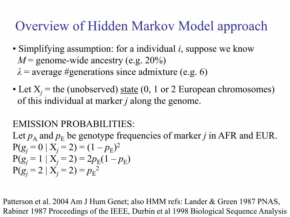
Overview of Hidden Markov Model approach
• Simplifying assumption: for a individual i, suppose we know
M = genome-wide ancestry (e.g. 20%)
λ = average #generations since admixture (e.g. 6)
• Let Xj = the (unobserved) state (0, 1 or 2 European chromosomes)
of this individual at marker j along the genome.
INITIAL PROBABILITIES (e.g. left end of chromosome):
TRANSITION PROBABILITIES
EMISSION PROBABILITIES
Patterson et al. 2004 Am J Hum Genet; also HMM refs: Lander & Green 1987 PNAS,
Rabiner 1987 Proceedings of the IEEE, Durbin et al 1998 Biological Sequence Analysis

Overview of Hidden Markov Model approach
• Simplifying assumption: for a individual i, suppose we know
M = genome-wide ancestry (e.g. 20%)
λ = average #generations since admixture (e.g. 6)
• Let Xj = the (unobserved) state (0, 1 or 2 European chromosomes)
of this individual at marker j along the genome.
INITIAL PROBABILITIES (e.g. left end of chromosome):
P(X0 = 0) = (1 – M)2
P(X0 = 1) = 2M(1 – M)
P(X0 = 2) = M2
Patterson et al. 2004 Am J Hum Genet; also HMM refs: Lander & Green 1987 PNAS,
Rabiner 1987 Proceedings of the IEEE, Durbin et al 1998 Biological Sequence Analysis

Overview of Hidden Markov Model approach
• Simplifying assumption: for a individual i, suppose we know
M = genome-wide ancestry (e.g. 20%)
λ = average #generations since admixture (e.g. 6)
• Let Xj = the (unobserved) state (0, 1 or 2 European chromosomes)
of this individual at marker j along the genome.
TRANSITION PROBABILITIES:
Let d be the genetic distance (in Morgans) between markers j and j+1.
P(Xj+1 = 0 | Xj = 0) = e–2λd + 2e–λd(1 – e–λd)(1 – M) + (1 – e–λd)2(1 – M)2
Patterson et al. 2004 Am J Hum Genet; also HMM refs: Lander & Green 1987 PNAS,
Rabiner 1987 Proceedings of the IEEE, Durbin et al 1998 Biological Sequence Analysis
0 of 2
chrom.
recombine
1 of 2
chrom.
recombine
2 of 2
chrom.
recombine

Overview of Hidden Markov Model approach
• Simplifying assumption: for a individual i, suppose we know
M = genome-wide ancestry (e.g. 20%)
λ = average #generations since admixture (e.g. 6)
• Let Xj = the (unobserved) state (0, 1 or 2 European chromosomes)
of this individual at marker j along the genome.
TRANSITION PROBABILITIES:
Let d be the genetic distance (in Morgans) between markers j and j+1.
P(Xj+1 = 0 | Xj = 0) = e–2λd + 2e–λd(1 – e–λd)(1 – M) + (1 – e–λd)2(1 – M)2
P(Xj+1 = 1 | Xj = 0) = 2e–λd(1 – e–λd)M + (1 – e–λd)22M(1 – M)
P(Xj+1 = 2 | Xj = 0) = (1 – e–λd)2M2
Patterson et al. 2004 Am J Hum Genet; also HMM refs: Lander & Green 1987 PNAS,
Rabiner 1987 Proceedings of the IEEE, Durbin et al 1998 Biological Sequence Analysis

Overview of Hidden Markov Model approach
• Simplifying assumption: for a individual i, suppose we know
M = genome-wide ancestry (e.g. 20%)
λ = average #generations since admixture (e.g. 6)
• Let Xj = the (unobserved) state (0, 1 or 2 European chromosomes)
of this individual at marker j along the genome.
TRANSITION PROBABILITIES:
Let d be the genetic distance (in Morgans) between markers j and j+1.
P(Xj+1 = 0 | Xj = 1) = 2e–λd(1 – e–λd)(1 – M) + (1 – e–λd)2(1 – M)2
P(Xj+1 = 1 | Xj = 1) = e–2λd + e–λd(1 – e–λd) + (1 – e–λd)22M(1 – M)
P(Xj+1 = 2 | Xj = 1) = e–λd(1 – e–λd)M + (1 – e–λd)2M2
Patterson et al. 2004 Am J Hum Genet; also HMM refs: Lander & Green 1987 PNAS,
Rabiner 1987 Proceedings of the IEEE, Durbin et al 1998 Biological Sequence Analysis

Overview of Hidden Markov Model approach
• Simplifying assumption: for a individual i, suppose we know
M = genome-wide ancestry (e.g. 20%)
λ = average #generations since admixture (e.g. 6)
• Let Xj = the (unobserved) state (0, 1 or 2 European chromosomes)
of this individual at marker j along the genome.
TRANSITION PROBABILITIES:
Let d be the genetic distance (in Morgans) between markers j and j+1.
P(Xj+1 = 0 | Xj = 2) = (1 – e–λd)2(1 – M)2
P(Xj+1 = 1 | Xj = 2) = 2e–λd(1 – e–λd)(1 – M) + (1 – e–λd)22M(1 – M)
P(Xj+1 = 2 | Xj = 2) = e–2λd + 2e–λd(1 – e–λd)M + (1 – e–λd)2M2
Patterson et al. 2004 Am J Hum Genet; also HMM refs: Lander & Green 1987 PNAS,
Rabiner 1987 Proceedings of the IEEE, Durbin et al 1998 Biological Sequence Analysis

Overview of Hidden Markov Model approach
• Simplifying assumption: for a individual i, suppose we know
M = genome-wide ancestry (e.g. 20%)
λ = average #generations since admixture (e.g. 6)
• Let Xj = the (unobserved) state (0, 1 or 2 European chromosomes)
of this individual at marker j along the genome.
EMISSION PROBABILITIES:
Let pA and pE be genotype frequencies of marker j in AFR and EUR.
P(gj = 0 | Xj = 0) = (1 – pA)2
P(gj = 1 | Xj = 0) = 2pA(1 – pA)
P(gj = 2 | Xj = 0) = pA2
Patterson et al. 2004 Am J Hum Genet; also HMM refs: Lander & Green 1987 PNAS,
Rabiner 1987 Proceedings of the IEEE, Durbin et al 1998 Biological Sequence Analysis

Overview of Hidden Markov Model approach
• Simplifying assumption: for a individual i, suppose we know
M = genome-wide ancestry (e.g. 20%)
λ = average #generations since admixture (e.g. 6)
• Let Xj = the (unobserved) state (0, 1 or 2 European chromosomes)
of this individual at marker j along the genome.
EMISSION PROBABILITIES:
Let pA and pE be genotype frequencies of marker j in AFR and EUR.
P(gj = 0 | Xj = 1) = (1 – pA)(1 – pE)
P(gj = 1 | Xj = 1) = pA(1 – pE) + pE(1 – pA)
P(gj = 2 | Xj = 1) = pApE
Patterson et al. 2004 Am J Hum Genet; also HMM refs: Lander & Green 1987 PNAS,
Rabiner 1987 Proceedings of the IEEE, Durbin et al 1998 Biological Sequence Analysis
Overview of Hidden Markov Model approach
• Simplifying assumption: for a individual i, suppose we know
M = genome-wide ancestry (e.g. 20%)
λ = average #generations since admixture (e.g. 6)
• Let Xj = the (unobserved) state (0, 1 or 2 European chromosomes)
of this individual at marker j along the genome.
EMISSION PROBABILITIES:
Let pA and pE be genotype frequencies of marker j in AFR and EUR.
P(gj = 0 | Xj = 2) = (1 – pE)2
P(gj = 1 | Xj = 2) = 2pE(1 – pE)
P(gj = 2 | Xj = 2) = pE2
Patterson et al. 2004 Am J Hum Genet; also HMM refs: Lander & Green 1987 PNAS,
Rabiner 1987 Proceedings of the IEEE, Durbin et al 1998 Biological Sequence Analysis

Overview of Hidden Markov Model approach
• Simplifying assumption: for a individual i, suppose we know
M = genome-wide ancestry (e.g. 20%)
λ = average #generations since admixture (e.g. 6)
• Let Xj = the (unobserved) state (0, 1 or 2 European chromosomes)
of this individual at marker j along the genome.
INITIAL PROBABILITIES (e.g. left end of chromosome):
TRANSITION PROBABILITIES
EMISSION PROBABILITIES
Then apply forward-backward algorithm to infer P(Xj | genotypes).
Patterson et al. 2004 Am J Hum Genet; also HMM refs: Lander & Green 1987 PNAS,
Rabiner 1987 Proceedings of the IEEE, Durbin et al 1998 Biological Sequence Analysis

Overview of Hidden Markov Model approach
Then apply forward-backward algorithm to infer P(Xj | genotypes).
P(X1|g1) P(Xj|g1…gj) P(XM-1|g1…gM-1) P(XM|g1…gM)
(FORWARD PROBABILITIES)
Durbin et al 1998 Biological Sequence Analysis

Overview of Hidden Markov Model approach
Then apply forward-backward algorithm to infer P(Xj | genotypes).
P(X1|g1) P(Xj|g1…gj) P(XM-1|g1…gM-1) P(XM|g1…gM)
(FORWARD PROBABILITIES)
P(g2…gM|X1) P(gj+1…gM|Xj) P(gM|XM-1) 1
(BACKWARD PROBABILITIES)
Durbin et al 1998 Biological Sequence Analysis

Overview of Hidden Markov Model approach
Then apply forward-backward algorithm to infer P(Xj | genotypes).
P(X1|g1) P(Xj|g1…gj) P(XM-1|g1…gM-1) P(XM|g1…gM)
P(g2…gM|X1) P(gj+1…gM|Xj) P(gM|XM-1) 1
P(X1|g1…gM) … P(Xj|g1…gM) … P(XM-1|g1…gM) P(XM|g1…gM)
Durbin et al 1998 Biological Sequence Analysis

Overview of Hidden Markov Model approach
• Simplifying assumption: for a individual i, suppose we know
M = genome-wide ancestry (e.g. 20%)
λ = average #generations since admixture (e.g. 6)
• Let Xj = the (unobserved) state (0, 1 or 2 European chromosomes)
of this individual at marker j along the genome.
INITIAL PROBABILITIES (e.g. left end of chromosome):
TRANSITION PROBABILITIES
EMISSION PROBABILITIES
Then apply forward-backward algorithm to infer P(Xj | genotypes).
(Or, use MCMC to integrate over uncertainty in M, λ, pA, pE.)
Patterson et al. 2004 Am J Hum Genet; also HMM refs: Lander & Green 1987 PNAS,
Rabiner 1987 Proceedings of the IEEE, Durbin et al 1998 Biological Sequence Analysis

Big trouble if markers are in LD in ancestral populations
Example: Admixed population with 80% POP1, 20% POP2 ancestry
SNP1 = A/C SNP, A allele has frequency 0.25 in POP1, 0.75 in POP2
A allele has frequency 80%·0.25 + 20%·0.75 = 0.35 in Admixed pop.
Inference of local ancestry of a haploid chromosome using SNP1:
prob 0.35: P(POP1 | A) = 80%·0.25/(80%·0.25 + 20%·0.75 ) = 57%
prob 0.65: P(POP1 | C) = 80%·0.75/(80%·0.75 + 20%·0.25) = 92%
Overall: P(POP1) = 57%·0.35 + 92%·0.65 = 80%. Unbiased.
Price et al. 2008 Am J Hum Genet

Big trouble if markers are in LD in ancestral populations
Example: Admixed population with 80% POP1, 20% POP2 ancestry
SNP1 = A/C SNP, A allele has frequency 0.25 in POP1, 0.75 in POP2
SNP2 = A/C SNP in perfect LD with SNP1 in POP1, POP2
A allele has frequency 80%·0.25 + 20%·0.75 = 0.35 in Admixed pop.
Inference of local ancestry of a haploid chr using SNP1, SNP2:
prob 0.35: P(POP1 | AA) = 80%·0.252/(80%·0.252 + 20%·0.752) =
31%
prob 0.65: P(POP1 | CC) = 80%·0.752/(80%·0.752 + 20%·0.252) =
97%
Overall: P(POP1) = 31%·0.35 + 97%·0.65 = 74%. Biased.
Price et al. 2008 Am J Hum Genet

Inferring local ancestry using GWAS chip data
Advantages of AIM panels of 1,500+ SNPs:
• Lower cost: $80/sample
(vs. $300+sample for GWAS chips).
Advantages of GWAS chips:
• Dense SNP coverage enables LD mapping
• More accurate local ancestry inference?

Inferring local ancestry using GWAS chip data
• ANCESTRYMAP using a subset of ~8,000 unlinked AIMs
(Patterson et al. 2004 Am J Hum Genet; Tandon et al. 2011 Genet Epidemiol)
New methods developed for GWAS chip data: • SABER (Tang et al. 2006 Am J Hum Genet)
• LAMP (Sankararaman et al. 2008 Am J Hum Genet)
• uSWITCH (Sankararaman et al. 2008 Genome Res)
• HAPAA (Sundquist et al. 2008 Genome Res)
• HAPMIX (Price, Tandon et al. 2009 PLoS Genet)
• WINPOP (Pasaniuc et al. 2009 Bioinformatics)
• GEDI-ADMX (Pasaniuc et al. 2009 Lect Notes Comput Sci)
• PCA-based method (Bryc, Auton et al. 2010 PNAS)
• LAMP-LD (Baran et al. 2012 Bioinformatics)
• MULTIMIX (Churchhouse & Marchini 2013 Genet Epidemiol)
• RFMix (Maples et al. 2013 Am J Hum Genet)
reviewed in Seldin et al. 2011 Nat Rev Genet

Inferring local ancestry using GWAS chip data
• ANCESTRYMAP using a subset of ~8,000 unlinked AIMs
(Patterson et al. 2004 Am J Hum Genet; Tandon et al. 2011 Genet Epidemiol)
New methods developed for GWAS chip data: • SABER (Tang et al. 2006 Am J Hum Genet)
• LAMP (Sankararaman et al. 2008 Am J Hum Genet) • uSWITCH (Sankararaman et al. 2008 Genome Res)
• HAPAA (Sundquist et al. 2008 Genome Res)
• HAPMIX (Price, Tandon et al. 2009 PLoS Genet) • WINPOP (Pasaniuc et al. 2009 Bioinformatics)
• GEDI-ADMX (Pasaniuc et al. 2009 Lect Notes Comput Sci)
• PCA-based method (Bryc, Auton et al. 2010 PNAS)
• LAMP-LD (Baran et al. 2012 Bioinformatics)
• MULTIMIX (Churchhouse & Marchini 2013 Genet Epidemiol)
• RFMix (Maples et al. 2013 Am J Hum Genet)
reviewed in Seldin et al. 2011 Nat Rev Genet

Inferring local ancestry: LAMP method
LAMP method: (allele frequencies in ancestral populations not known)
• Prune SNP set to restrict to unlinked markers (r2 < 0.10)
• Choose fixed window length l
• Infer local ancestry within each window of length l via EM algorithm
(Unsupervised clustering, integer-valued haploid local ancestries)
• For each SNP, compute majority vote of local ancestry across
all windows overlapping that SNP.
Sankararaman et al. 2008 Am J Hum Genet
1
2
3
4
5
6
7
Window window length l

Inferring local ancestry: LAMP-ANC method
LAMP-ANC: (allele frequencies in ancestral populations are known)
• Prune SNP set to restrict to unlinked markers (r2 < 0.10)
• Choose fixed window length l
• Infer local ancestry within each window of length l via max likelihood
(Supervised clustering, integer-valued haploid local ancestries)
• For each SNP, compute majority vote of local ancestry across
all windows overlapping that SNP.
Sankararaman et al. 2008 Am J Hum Genet
1
2
3
4
5
6
7
Window window length l

Inferring local ancestry: LAMP and LAMP-ANC
LAMP and LAMP-ANC:
• Prune SNP set to restrict to unlinked markers (r2 < 0.10)
• Choose fixed window length l
• Infer local ancestry within each window of length l
• For each SNP, compute majority vote across windows containing SNP
Choice of window length l is key. If window length is
• too small: not enough information to infer local ancestry
• too big: violates assumption of constant local ancestry within window
window length l
Sankararaman et al. 2008 Am J Hum Genet

Inferring local ancestry: LAMP and LAMP-ANC
LAMP and LAMP-ANC:
• Prune SNP set to restrict to unlinked markers (r2 < 0.10)
• Choose fixed window length l
• Infer local ancestry within each window of length l
• For each SNP, compute majority vote across windows containing SNP
Choice of window length l is key. If window length is
• too small: not enough information to infer local ancestry
• too big: violates assumption of constant local ancestry within window
Use window length l which is
inversely proportional to # generations since admixture,
i.e. proportional to ancestry segment lengths
window length l
Sankararaman et al. 2008 Am J Hum Genet

Inferring local ancestry: LAMP and LAMP-ANC
LAMP and LAMP-ANC:
• Prune SNP set to restrict to unlinked markers (r2 < 0.10)
• Choose fixed window length l
• Infer local ancestry within each window of length l
• For each SNP, compute majority vote across windows containing SNP
Advantages:
• Simple and transparent approach, low computational cost
Disadvantages:
• Information from neighboring windows is not used
• Does not make use of haplotype information
window length l
Sankararaman et al. 2008 Am J Hum Genet
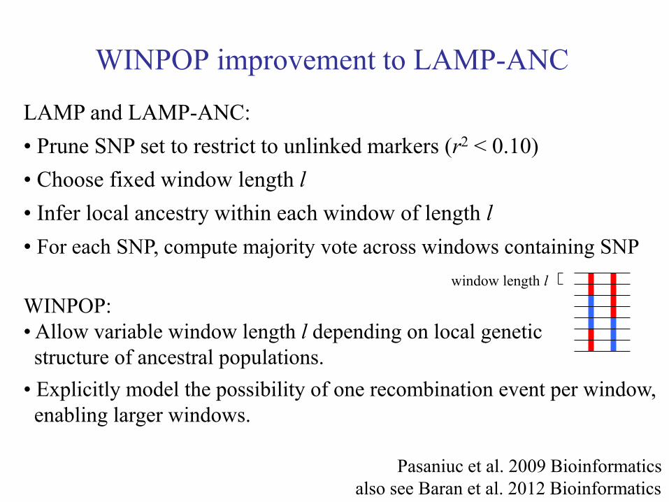
WINPOP improvement to LAMP-ANC
LAMP and LAMP-ANC:
• Prune SNP set to restrict to unlinked markers (r2 < 0.10)
• Choose fixed window length l
• Infer local ancestry within each window of length l
• For each SNP, compute majority vote across windows containing SNP
WINPOP:
• Allow variable window length l depending on local genetic
structure of ancestral populations.
• Explicitly model the possibility of one recombination event per window,
enabling larger windows.
window length l
Pasaniuc et al. 2009 Bioinformatics
also see Baran et al. 2012 Bioinformatics

Inferring local ancestry: HAPMIX method
HAPMIX method: nested Hidden Markov Models
• Large-scale HMM: transitions between local ancestry states
(Patterson et al. 2004 Am J Hum Genet).
• Small-scale HMM: transitions between haplotypes from
ancestral reference populations (Li & Stephens 2003 Genetics)
Price, Tandon et al. 2009 PLoS Genet
POP1
POP2
hap1
hap2
hap3
hap4
hap5
hap1
hap2
hap3
hap4
hap5

Inferring local ancestry: HAPMIX method
HAPMIX method: nested Hidden Markov Models
• States: local ancestry AND haplotype from POP1 or POP2.
• Given initial, transition and emission probabilities: use
forward-backward algorithm to infer P(states | data).
(Durbin et al. 1998 Biological Sequence Analysis + other HMM refs)
Price, Tandon et al. 2009 PLoS Genet
POP1
POP2
hap1
hap2
hap3
hap4
hap5
hap1
hap2
hap3
hap4
hap5

Inferring local ancestry: HAPMIX method
Advantages:
• Large-scale + Small-scale HMM use all information in GWAS chip data
Disadvantages:
• Increased complexity and running time
POP1
POP2
hap1
hap2
hap3
hap4
hap5
hap1
hap2
hap3
hap4
hap5
Price, Tandon et al. 2009 PLoS Genet

Next steps to understanding local ancestry inference
Rhythm is gonna get you.
-- Gloria S.
Data is gonna get you.
-- Alkes

Example on real data actual chr1 local ancestry of one African-American sample,
estimated by HAPMIX, ANCESTRYMAP, LAMP
Price, Tandon et al. 2009 PLoS Genet

Johnson et al. 2011 PLoS Genet
also see Moreno-Estrada et al. 2013 PLoS Genet, Gravel et al. 2013 PLoS Genet

Johnson et al. 2011 PLoS Genet
also see Moreno-Estrada et al. 2013 PLoS Genet, Gravel et al. 2013 PLoS Genet

Other uses of local ancestry information
(besides population genetics)
Freedman et al. 2006 PNAS
also see Seldin et al. 2011 Nat Rev Genet
Genovese et al. 2013 Nat Genet
also see Genovese et al. 2013 Am J Hum Genet
Zaitlen et al. 2014 Nat Genet
Outline
1. Admixture leads to variation in genome-wide ancestry
2. Admixture creates mosaic chromosomes
3. Local ancestry inference
4. Evaluating local ancestry inference algorithms

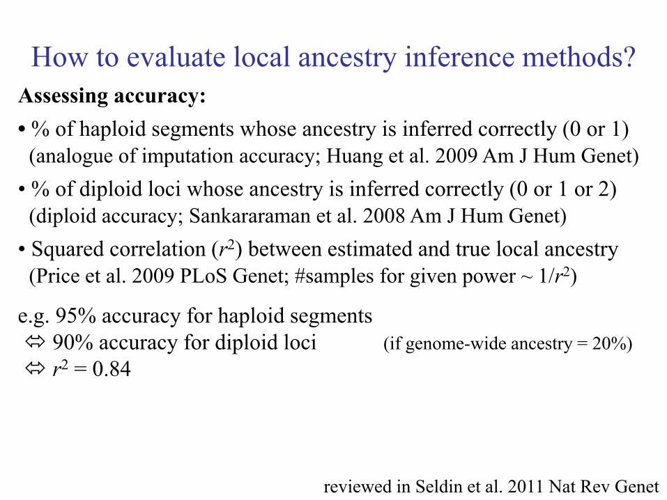
How to evaluate local ancestry inference methods?
• % of haploid segments whose ancestry is inferred correctly (0 or 1)
(analogue of imputation accuracy; Huang et al. 2009 Am J Hum Genet)
• % of diploid loci whose ancestry is inferred correctly (0 or 1 or 2)
(diploid accuracy; Sankararaman et al. 2008 Am J Hum Genet)
• Squared correlation (r2) between estimated and true local ancestry
(Price et al. 2009 PLoS Genet; #samples for given power ~ 1/r2)
Assessing accuracy:
reviewed in Seldin et al. 2011 Nat Rev Genet
How to evaluate local ancestry inference methods?
• % of haploid segments whose ancestry is inferred correctly (0 or 1)
(analogue of imputation accuracy; Huang et al. 2009 Am J Hum Genet)
• % of diploid loci whose ancestry is inferred correctly (0 or 1 or 2)
(diploid accuracy; Sankararaman et al. 2008 Am J Hum Genet)
• Squared correlation (r2) between estimated and true local ancestry
(Price et al. 2009 PLoS Genet; #samples for given power ~ 1/r2)
e.g. 95% accuracy for haploid segments
90% accuracy for diploid loci (if genome-wide ancestry = 20%)
r2 = 0.84
Assessing accuracy:
reviewed in Seldin et al. 2011 Nat Rev Genet

How to evaluate local ancestry inference methods?
• % of haploid segments whose ancestry is inferred correctly (0 or 1)
(analogue of imputation accuracy; Huang et al. 2009 Am J Hum Genet)
• % of diploid loci whose ancestry is inferred correctly (0 or 1 or 2)
(diploid accuracy; Sankararaman et al. 2008 Am J Hum Genet)
• Squared correlation (r2) between estimated and true local ancestry
(Price et al. 2009 PLoS Genet; #samples for given power ~ 1/r2)
Simulated African Americans with 6 generations since admixture:
ANCESTRYMAP r2 = 0.83
LAMP r2 = 0.84
WINPOP r2 = 0.94
HAPMIX r2 = 0.98
Assessing accuracy:
reviewed in Seldin et al. 2011 Nat Rev Genet

How to evaluate local ancestry inference methods?
Even more important than assessing accuracy: no spurious peaks
Average HAPMIX local ancestry estimates of 6,209 AA from CARe
HAPMIX
Pasaniuc et al. PLoS Genet 2011;
also see Price, Tandon et al. 2009 PLoS Genet
slide repeated in Week 4 bonus slides

How to evaluate local ancestry inference methods?
Even more important than assessing accuracy: no spurious peaks
Average ANCESTRYMAP local ancestry estimates of CARe AA
Admixture peaks should be evaluated
using two independent algorithms
(Reich et al. 2005 Phil Trans R Soc B)
Pasaniuc et al. PLoS Genet 2011
Tandon et al. 2011 Genet Epidemiol

Latino populations: 3-way admixture
Bryc, Velez et al. 2010 PNAS
European
Native American
African

Local ancestry inference in Latino populations
Main challenge:
• Lack of accurate Native American ancestral reference panels
can lead to spurious deviations in local ancestry
Additional challenges:
• Some local ancestry algorithms do not support 3-way admixture
• Native American reference panels may themselves be admixed
• European reference panels: N. Europe panels may be inaccurate
reference population for S. Europe ancestral population
Seldin et al. 2011 Nat Rev Genet
Pasaniuc et al. 2013 Bioinformatics
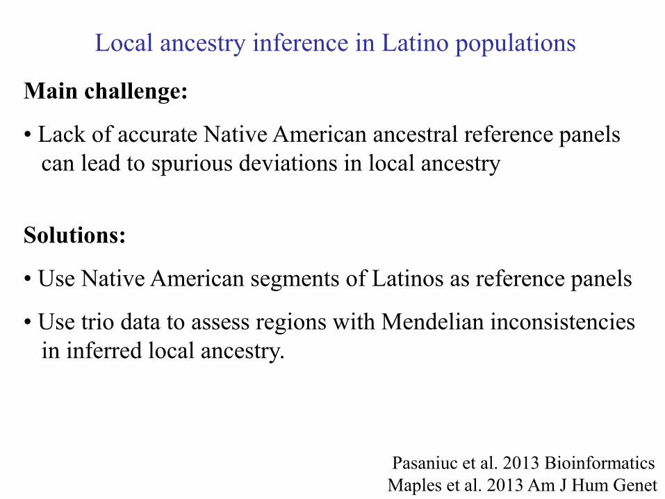
Local ancestry inference in Latino populations
Main challenge:
• Lack of accurate Native American ancestral reference panels
can lead to spurious deviations in local ancestry
Solutions:
• Use Native American segments of Latinos as reference panels
• Use trio data to assess regions with Mendelian inconsistencies
in inferred local ancestry.
Pasaniuc et al. 2013 Bioinformatics
Maples et al. 2013 Am J Hum Genet

• In an admixed population, different people have different
genome-wide ancestry proportions.
• Each individual from an admixed population has mosaic
chromosomes with segments of different continental ancestry.
These mosaic chromosomes lead to admixture-LD.
• Local ancestry can be inferred from AIM panels with decent
accuracy and from GWAS chip data with high accuracy.
• Local ancestry inference accuracy can be evaluated using r2
and lack of spurious peaks in large empirical data sets.
Conclusions

Outline
1. Admixture leads to variation in genome-wide ancestry
2. Admixture creates mosaic chromosomes
3. Local ancestry inference
4. Evaluating local ancestry inference algorithms
Bonus: extra content on admixture mapping

Outline (admixture mapping)
1. Introduction to admixture mapping
2. Admixture mapping statistics: case-control and case-only
3. Real examples of admixture mapping studies
4. Admixture association vs. SNP association

Outline (admixture mapping)
1. Introduction to admixture mapping
2. Admixture mapping statistics: case-control and case-only
3. Real examples of admixture mapping studies
4. Admixture association vs. SNP association

Autosomal recessive diseases (genetic):
Cystic fibrosis ( European ancestry)
Sickle-cell anemia ( African ancestry)
Background: population differences in disease

Autosomal recessive diseases (genetic):
Cystic fibrosis ( European ancestry)
Sickle-cell anemia ( African ancestry)
Complex diseases (genetic and/or environmental):
Multiple sclerosis ( European ancestry)
Prostate cancer ( African ancestry)
Type 2 diabetes ( Native American ancestry)
African Americans: African + European ancestry
Latinos: European + Native American + African ancestry
Background: population differences in disease

Using admixture to map disease
Admixture association: a location of the genome
where average local ancestry in disease cases has an
unusual deviation.

Using admixture to map disease:
toy example
Example: HBB gene (risk locus for sickle-cell anemia)
• Sickle-cell mutation exists at allele frequency
0%* in European populations, 5%* in African populations.
[mutations on both chromosomes => sickle-cell anemia]
• Local ancestry of African American chromosomes at HBB:
20% have European local ancestry
76% have African local ancestry without sickle-cell mutation
4% have African local ancestry with sickle-cell mutation
Mears et al. 1981 J Clin Invest

Using admixture to map disease:
toy example
100%
75%
50%
African Americans with sickle-cell anemia have
100 % African ancestry at HBB locus.
Position in the genome

Using admixture to map disease:
toy example #2
Example: CFTR gene (risk locus for cystic fibrosis)
• Cystic fibrosis mutations exist at allele frequency
2%* in European populations, 0%* in African populations.
[mutations on both chromosomes => cystic fibrosis]
• Local ancestry of African American chromosomes at CFTR:
80% have African local ancestry
19.6% have European local ancestry without CFTR mutation
0.4% have European local ancestry with CFTR mutation
Morton 1968 Am J Hum Genet

Using admixture to map disease:
toy example #2
100%
50%
0%
African Americans with cystic fibrosis have
0% African ancestry at CFTR locus.
Position in the genome

100%
75%
50%
Position in the genome
African Americans with common disease X have
higher % African ancestry at disease locus.
Using admixture to map disease:
realistic example

100%
75%
50%
Position in the genome
African Americans with common disease X have
higher % African ancestry at disease locus.
• Risk allele has higher freq in Africans than Europeans
• disease is more common in Africans than Europeans
Using admixture to map disease:
realistic example
Disease locus

Admixture association is different
from SNP association
• Requires fewer markers, since local ancestry can be
inferred using <2,000 ancestry-informative markers
(Smith et al. 2004 Am J Hum Genet, Tian et al. 2006 Am J Hum Genet)
• Poor localization: admixture association signal spans
several megabases.
• Lower multiple hypothesis testing burden than GWAS:
effective number of regions tested is only hundreds.
• Does not require data from controls (case-only statistics).

LD enables (indirect) SNP association …
Admixture-LD enables admixture association
Real example of admixture-LD:
rs164781: 0.42 in CEU, 0.88 in YRI (HapMap3)
rs10495758: 0.88 in CEU, 0.32 in YRI (HapMap3)
These SNPs are located roughly 3Mb apart.
r2 between rs164781 and rs10495758:
0.01 in CEU, 0.01 in YRI, 0.28 in ASW (HapMap3)
rs164781 and rs10495758 are in admixture-LD in ASW!
(from Week 4)
International HapMap3 Consortium 2010 Nature
SNPs chosen from Tandon et al. 2011 Genet Epidemiol
Outline
1. Introduction to admixture mapping
2. Admixture mapping statistics: case-control and case-only
3. Real examples of admixture mapping studies
4. Admixture association vs. SNP association

Case-control admixture association
Case-control admixture association: a location of the
genome where average local ancestry in disease cases
has an unusual deviation compared to average
local ancestry in controls.
Case-control admixture association, simplified
• Armitage Trend Test for case-control SNP association:
Nρ(genotype at candidate SNP, phenotype)2
Armitage 1955 Biometrics

Case-control admixture association, simplified
• Armitage Trend Test for case-control SNP association:
Nρ(genotype at candidate SNP, phenotype)2
• Armitage Trend Test for case-control admixture association:
Nρ(local ancestry at candidate locus, phenotype)2
Armitage 1955 Biometrics
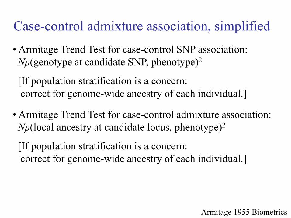
Case-control admixture association, simplified
• Armitage Trend Test for case-control SNP association:
Nρ(genotype at candidate SNP, phenotype)2
[If population stratification is a concern:
correct for genome-wide ancestry of each individual.]
• Armitage Trend Test for case-control admixture association:
Nρ(local ancestry at candidate locus, phenotype)2
[If population stratification is a concern:
correct for genome-wide ancestry of each individual.]
Armitage 1955 Biometrics

Toy example: Admixed population with 50% POP1, 50% POP2.
SNP1 = A/C SNP, A allele has frequency 0.10 in POP1, 0.90 in POP2
Suppose that SNP1 is the causal variant, with Odds Ratio = 1.5.
Case-control admixture association: toy example

Toy example: Admixed population with 50% POP1, 50% POP2.
SNP1 = A/C SNP, A allele has frequency 0.10 in POP1, 0.90 in POP2
Suppose that SNP1 is the causal variant, with Odds Ratio = 1.5.
Probabilities of values of SNP1 and local ancestry:
Controls: P(SNP1=A) = 0.50 Cases: P(SNP1=A) = 0.60
P(SNP1=A, POP1) = 0.05 P(SNP1=A, POP1) = 0.06
P(SNP1=A, POP2) = 0.45 P(SNP1=A, POP2) = 0.54
P(SNP1=C, POP1) = 0.45 P(SNP1=C, POP1) = 0.36
P(SNP1=C, POP2) = 0.05 P(SNP1=C, POP2) = 0.04
P(POP2) = 0.50 P(POP2) = 0.58
Thus, there is a case-control admixture association at this locus.
Case-control admixture association: toy example
slide repeated in Week 6

Toy example: Admixed population with 50% POP1, 50% POP2.
SNP1 = A/C SNP, A allele has frequency 0.10 in POP1, 0.90 in POP2
Suppose that SNP1 is the causal variant, with Odds Ratio = 1.5.
Probabilities of values of SNP1 and local ancestry:
Controls: P(SNP1=A) = 0.50 Cases: P(SNP1=A) = 0.60
P(SNP1=A, POP1) = 0.05 P(SNP1=A, POP1) = 0.06
P(SNP1=A, POP2) = 0.45 P(SNP1=A, POP2) = 0.54
P(SNP1=C, POP1) = 0.45 P(SNP1=C, POP1) = 0.36
P(SNP1=C, POP2) = 0.05 P(SNP1=C, POP2) = 0.04
P(POP2) = 0.50 P(POP2) = 0.58
Thus, there is a case-control admixture association at this locus.
To detect admixture association: necessary to infer local ancestry,
but not necessary to genotype SNP1.
Case-control admixture association: toy example

SNP odds ratio vs. Ancestry odds ratio
Recall: The SNP odds ratio R is the ratio of ref vs. var alleles in
disease cases as compared to ref vs. var alleles in controls.
ref var Equivalently,
Controls: p : 1–p pcase(1 – pcontrol)
Cases: Rp : 1–p pcontrol(1 – pcase)
[Or, the SNP odds ratio R is the ratio of case vs. control odds for
ref allele as compared to case vs. control odds for var allele.]
R =
slide repeated in Week 6

SNP odds ratio vs. Ancestry odds ratio
Definition: The ancestry odds ratio Ω is the ratio of
European vs. African chromosomes in disease cases as compared
to European vs. African chromosomes in controls.
European African Equivalently,
Controls: γ : 1–γ γcase(1 – γcontrol)
Cases: Ωγ : 1–γ γcontrol(1 – γcase)
[Or, the ancestry odds ratio Ω is the ratio of case vs. control odds
for Eur chr as compared to case vs. control odds for Afr chr.]
Ω =
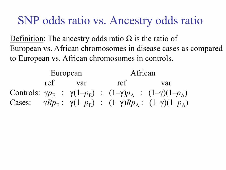
SNP odds ratio vs. Ancestry odds ratio
Definition: The ancestry odds ratio Ω is the ratio of
European vs. African chromosomes in disease cases as compared
to European vs. African chromosomes in controls.
European African
ref var ref var
Controls: γpE : γ(1–pE) : (1–γ)pA : (1–γ)(1–pA)
Cases: γRpE : γ(1–pE) : (1–γ)RpA : (1–γ)(1–pA)

SNP odds ratio vs. Ancestry odds ratio
Definition: The ancestry odds ratio Ω is the ratio of
European vs. African chromosomes in disease cases as compared
to European vs. African chromosomes in controls.
European (ref + var) African (ref + var)
Controls: γ : 1–γ
Cases: γ(RpE + 1–pE) : (1–γ)(RpA + 1–pA)
This implies that the ancestry odds ratio Ω is equal to
RpE + 1–pE
RpA + 1–pA

SNP odds ratio vs. Ancestry odds ratio
The ancestry odds ratio Ω is equal to
RpE + 1–pE
RpA + 1–pA
R pE pA Ω
1.50 100% 0% 1.50
1.50 0% 100% 0.67
1.50 90% 10% 1.38
1.50 75% 25% 1.22
1.50 60% 40% 1.08
1.50 50% 50% 1.00
(see toy example)

Case-only admixture association
Case-only admixture association: a location of the
genome where average local ancestry in disease cases
has an unusual deviation compared to local ancestry
in the same disease cases elsewhere in the genome.

Case-only admixture association
Case-only admixture association: a location of the
genome where average local ancestry in disease cases
has an unusual deviation compared to local ancestry
in the same disease cases elsewhere in the genome.
Case-only (a.k.a. locus-genome) admixture statistics are
more powerful than case-control statistics, due to the
lack of statistical noise introduced from controls.
Patterson et al. 2004 Am J Hum Genet

Case-only admixture association
Case-only admixture association: a location of the
genome where average local ancestry in disease cases
has an unusual deviation compared to local ancestry
in the same disease cases elsewhere in the genome.
Case-only (a.k.a. locus-genome) admixture statistics
require no deviations in average local ancestry in controls
(e.g. due to artifacts, selection since admixture, etc.)
Patterson et al. 2004 Am J Hum Genet

Case-only admixture statistics require no spurious peaks
Even more important than assessing accuracy: no spurious peaks
Average HAPMIX local ancestry estimates of 6,209 AA from CARe
HAPMIX
Pasaniuc et al. PLoS Genet 2011;
also see Price, Tandon et al. 2009 PLoS Genet (from Week 4)
Case-only admixture association, simplified
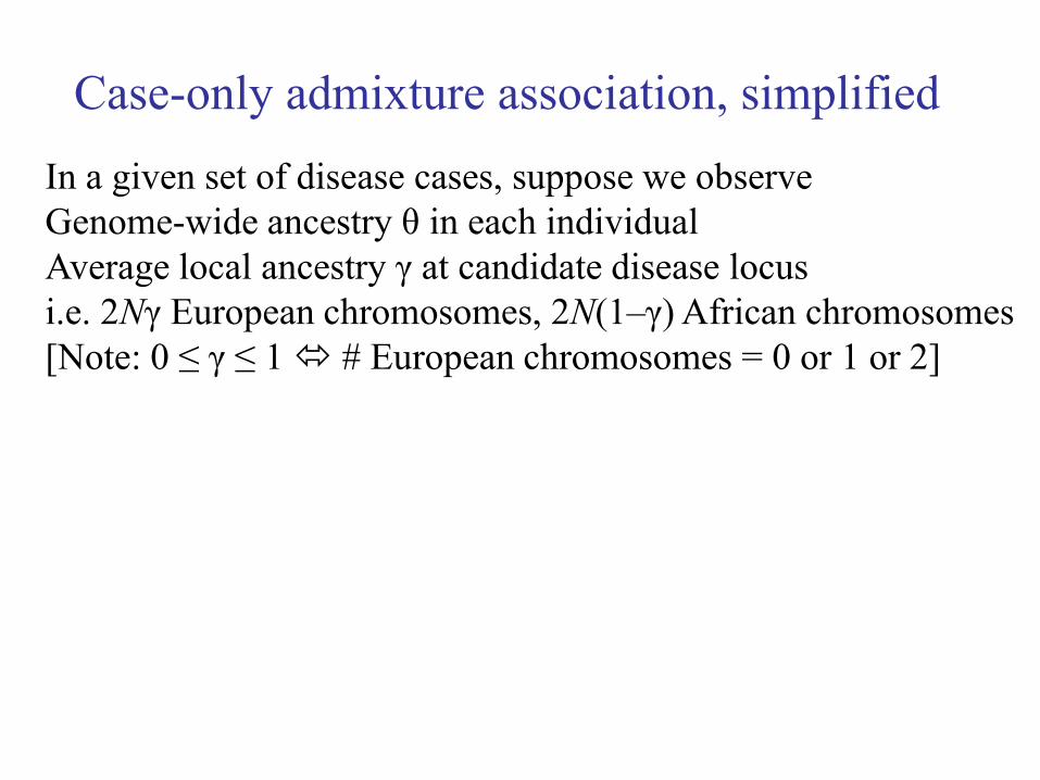
In a given set of disease cases, suppose we observe
Genome-wide ancestry θ in each individual
Average local ancestry γ at candidate disease locus
i.e. 2Nγ European chromosomes, 2N(1–γ) African chromosomes
[Note: 0 ≤ γ ≤ 1 # European chromosomes = 0 or 1 or 2]

Case-only admixture association, simplified
In a given set of disease cases, suppose we observe
Genome-wide ancestry θ in each individual
Average local ancestry γ at candidate disease locus
i.e. 2Nγ European chromosomes, 2N(1–γ) African chromosomes
NULL MODEL (γ* = θ):
log P(data | NULL) = 2Nγlog(θ) + 2N(1–γ)log(1–θ)
CAUSAL MODEL (γ* ≠ θ, highest likelihood at γ* = γ):
log P(data | CAUSAL) = 2Nγlog(γ) + 2N(1–γ)log(1–γ)
Note: all logs are loge unless otherwise indicated

Case-only admixture association, simplified
In a given set of disease cases, suppose we observe
Genome-wide ancestry θ in each individual
Average local ancestry γ at candidate disease locus
i.e. 2Nγ European chromosomes, 2N(1–γ) African chromosomes
NULL MODEL (γ* = θ):
log P(data | NULL) = 2Nγlog(θ) + 2N(1–γ)log(1–θ)
CAUSAL MODEL (γ* ≠ θ, highest likelihood at γ* = γ):
log P(data | CAUSAL) = 2Nγlog(γ) + 2N(1–γ)log(1–γ)
Likelihood-ratio test, χ2(1 dof):
2[2Nγlog(γ/θ) + 2N(1–γ)log((1–γ)/(1–θ))]

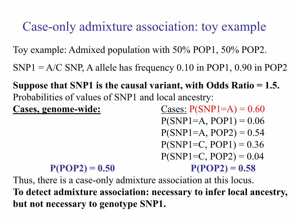
Toy example: Admixed population with 50% POP1, 50% POP2.
SNP1 = A/C SNP, A allele has frequency 0.10 in POP1, 0.90 in POP2
Suppose that SNP1 is the causal variant, with Odds Ratio = 1.5.
Case-only admixture association: toy example

Toy example: Admixed population with 50% POP1, 50% POP2.
SNP1 = A/C SNP, A allele has frequency 0.10 in POP1, 0.90 in POP2
Suppose that SNP1 is the causal variant, with Odds Ratio = 1.5.
Probabilities of values of SNP1 and local ancestry:
Cases, genome-wide: Cases: P(SNP1=A) = 0.60
P(SNP1=A, POP1) = 0.06
P(SNP1=A, POP2) = 0.54
P(SNP1=C, POP1) = 0.36
P(SNP1=C, POP2) = 0.04
P(POP2) = 0.50 P(POP2) = 0.58
Thus, there is a case-only admixture association at this locus.
θ = 0.50, γ = 0.58 => χ2(1 dof) = 0.051·N,
assuming N diploid disease cases and γ equal to its expected value.
Case-only admixture association: toy example

Toy example: Admixed population with 50% POP1, 50% POP2.
SNP1 = A/C SNP, A allele has frequency 0.10 in POP1, 0.90 in POP2
Suppose that SNP1 is the causal variant, with Odds Ratio = 1.5.
Probabilities of values of SNP1 and local ancestry:
Cases, genome-wide: Cases: P(SNP1=A) = 0.60
P(SNP1=A, POP1) = 0.06
P(SNP1=A, POP2) = 0.54
P(SNP1=C, POP1) = 0.36
P(SNP1=C, POP2) = 0.04
P(POP2) = 0.50 P(POP2) = 0.58
Thus, there is a case-only admixture association at this locus.
θ = 0.50, γ = 0.58 => χ2(1 dof) = 0.051·N (for N diploid disease cases)
vs. SNP case-control χ2(1 dof) = 0.040·N (for N cases, N controls)
Case-only admixture association: toy example
Toy example: Admixed population with 50% POP1, 50% POP2.
SNP1 = A/C SNP, A allele has frequency 0.10 in POP1, 0.90 in POP2
Suppose that SNP1 is the causal variant, with Odds Ratio = 1.5.
Probabilities of values of SNP1 and local ancestry:
Cases, genome-wide: Cases: P(SNP1=A) = 0.60
P(SNP1=A, POP1) = 0.06
P(SNP1=A, POP2) = 0.54
P(SNP1=C, POP1) = 0.36
P(SNP1=C, POP2) = 0.04
P(POP2) = 0.50 P(POP2) = 0.58
Thus, there is a case-only admixture association at this locus.
To detect admixture association: necessary to infer local ancestry,
but not necessary to genotype SNP1.
Case-only admixture association: toy example

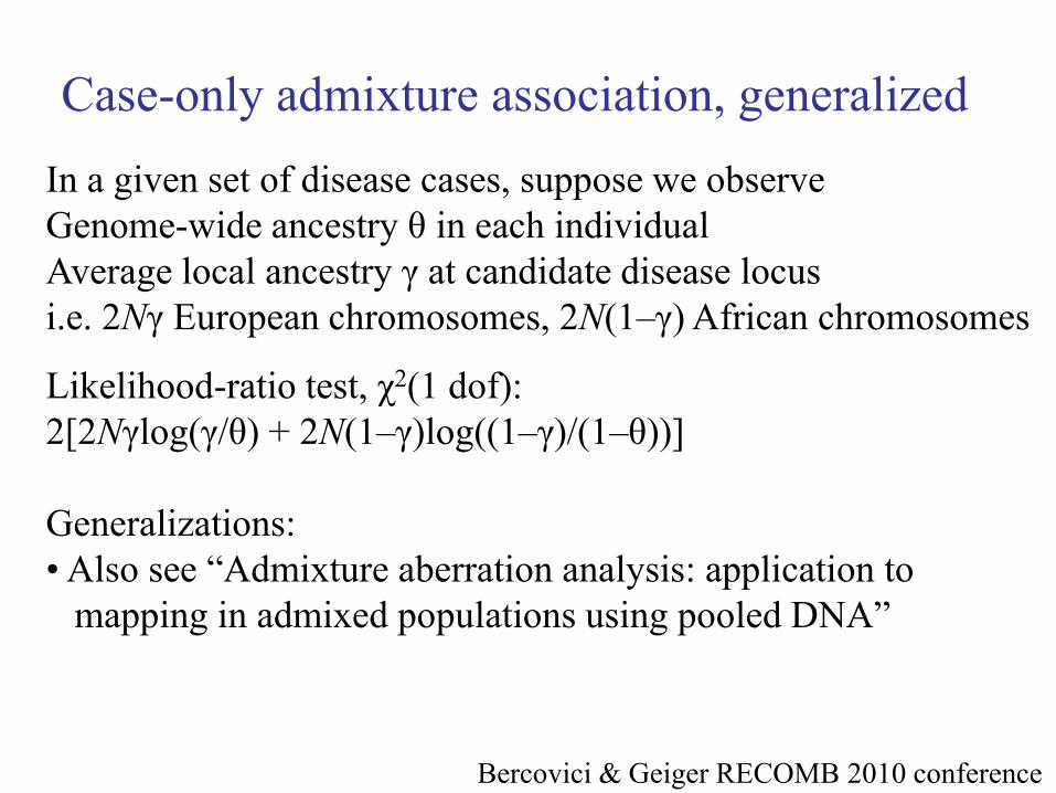
Case-only admixture association, generalized
In a given set of disease cases, suppose we observe
Genome-wide ancestry θ in each individual
Average local ancestry γ at candidate disease locus
i.e. 2Nγ European chromosomes, 2N(1–γ) African chromosomes
Likelihood-ratio test, χ2(1 dof):
2[2Nγlog(γ/θ) + 2N(1–γ)log((1–γ)/(1–θ))]
Generalizations:

In a given set of disease cases, suppose we observe
Genome-wide ancestry θ in each individual
Average local ancestry γ at candidate disease locus
i.e. 2Nγ European chromosomes, 2N(1–γ) African chromosomes
Likelihood-ratio test, χ2(1 dof):
2[2Nγlog(γ/θ) + 2N(1–γ)log((1–γ)/(1–θ))]
Generalizations:
• Different θi for each disease case i. [Ω relates θi to γi.]
Case-only admixture association, generalized

In a given set of disease cases, suppose we observe
Genome-wide ancestry θ in each individual
Average local ancestry γ at candidate disease locus
i.e. 2Nγ European chromosomes, 2N(1–γ) African chromosomes
Likelihood-ratio test, χ2(1 dof):
2[2Nγlog(γ/θ) + 2N(1–γ)log((1–γ)/(1–θ))]
Generalizations:
• Different θi for each disease case i. [Ω relates θi to γi.]
• Explicit probabilities for 0, 1 or 2 European chromosomes.
• ANCESTRYMAP approach: use MCMC to integrate over
uncertainty in θi and uncertainty in local ancestry estimates.
Patterson et al. 2004 Am J Hum Genet
Case-only admixture association, generalized
In a given set of disease cases, suppose we observe
Genome-wide ancestry θ in each individual
Average local ancestry γ at candidate disease locus
i.e. 2Nγ European chromosomes, 2N(1–γ) African chromosomes
Likelihood-ratio test, χ2(1 dof):
2[2Nγlog(γ/θ) + 2N(1–γ)log((1–γ)/(1–θ))]
Generalizations:
• Also see “Admixture aberration analysis: application to
mapping in admixed populations using pooled DNA”
Bercovici & Geiger RECOMB 2010 conference
Case-only admixture association, generalized
Next steps to understanding admixture mapping
Rhythm is gonna get you.
-- Gloria S.
Data is gonna get you.
-- Alkes

Outline
1. Introduction to admixture mapping
2. Admixture mapping statistics: case-control and case-only
3. Real examples of admixture mapping studies
4. Admixture association vs. SNP association

100%
75%
50%
Position in the genome
African Americans with prostate cancer have
higher % African ancestry at 8q24 disease locus.
Using admixture to map disease:
prostate cancer
Freedman et al. 2006 PNAS
LOD (log10 odds) score = 7.14

100%
75%
50%
Position in the genome
African Americans with prostate cancer have
higher % African ancestry at 8q24 disease locus.
Ancestry risk Ω=1.54 at 8q24 is sufficient to explain
higher rate of prostate cancer in African Americans.
Admixture peak spans position 125-130Mb on chr8.
Using admixture to map disease:
prostate cancer
Freedman et al. 2006 PNAS
LOD (log10 odds) score = 7.14
slide repeated in Week 6 bonus slides

100%
75%
50%
Position in the genome
African Americans with prostate cancer have
higher % African ancestry at 8q24 disease locus.
rs6983561, a SNP associated to prostate cancer,
has frequency 3% in Europeans but frequency
58% in Africans.
Using admixture to map disease:
prostate cancer
Freedman et al. 2006 PNAS
Haiman et al. 2007 Nat Genet
LOD (log10 odds) score = 7.14
slide repeated in Week 6 bonus slides

Using admixture to map disease:
multiple sclerosis
Reich et al. 2005 Nat Genet
LOD (log10 odds) score = 5.2

Using admixture to map disease:
multiple sclerosis
Reich et al. 2005 Nat Genet
LOD (log10 odds) score = 5.2
Ancestry effect at chr1 locus is
sufficient to explain lower rate
of MS in African Americans

Using admixture to map disease:
hypertension
Zhu et al. 2005 Nat Genet
Z score > 4
chr 6q
Z score > 4
chr 21q

Using admixture to map disease:
hypertension
Zhu et al. 2005 Nat Genet
Deo et al. 2007 PLoS Genet
Z score > 4
chr 6q
Z score > 4
chr 21q

Using admixture to map disease:
low white blood cell (WBC) count
Nalls et al. 2007 Am J Hum Genet
also see Reich et al. 2009 PLoS Genet
LOD (log10 odds) score > 20
chr 1q

Using admixture to map disease:
low white blood cell (WBC) count
Nalls et al. 2007 Am J Hum Genet
also see Reich et al. 2009 PLoS Genet
LOD (log10 odds) score > 20
chr 1q
Ancestry effect at chr1 locus is
sufficient to explain lower WBC
in African Americans
slide repeated in Week 6 bonus slides

LOD (log10 odds) score = 8.56
chr 22q
Using admixture to map disease:
End-stage renal disease Ancestry effect at chr22 locus is
sufficient to explain higher rate
of ESRD in African Americans
Kao et al. 2008 Nat Genet
also see Kopp et al. 2008 Nat Genet, Genovese et al. 2010 Science
slide repeated in Week 6 bonus slides

Yang, Cheng et al. 2011 Nat Genet
Disease phenotype: relapse of ALL
(acute lymphoblastic leukemia)
Case-control admixture association.
Using admixture to map disease:
relapse of ALL in a multi-ethnic U.S. cohort

Yang, Cheng et al. 2011 Nat Genet
Population stratification???
Dangers of population stratification in
case-control admixture association studies
Disease phenotype: relapse of ALL
(acute lymphoblastic leukemia)
Fejerman et al. 2012 Hum Mol Genet
Use admixture to map disease:
breast cancer in US Latinas
Disease phenotype: Breast cancer
US Latinas: higher European ancestry => higher risk,
even after correcting for known non-genetic risk factors.
6q25 locus: ancestry odds ratio 0.75 per Native American chr,
95% confidence interval 0.65-0.85, Pcorrected = 0.02.
“We evaluated significance via a permutation test.
Case/control status was permuted to reproduce the asymmetry
of the global ancestry distribution between cases and controls.

Outline
1. Introduction to admixture mapping
2. Admixture mapping statistics: case-control and case-only
3. Real examples of admixture mapping studies
4. Admixture association vs. SNP association
Admixture association vs. SNP association
“The idea of mapping disease using admixture techniques has
been around for ages, but is probably one whose time has come
and gone, before having any useful successes ... it no longer
has a strong rationale in an age when genotype costs have
fallen so dramatically and the typing of 100's of thousands of
SNPs from throughout the genome is often comparable to
typing smaller more painstakingly selected SNP pools.”
–Anonymous reviewer
(Price et al. 2007 Am J Hum Genet)

Admixture association vs. SNP association
• Can often be carried out using <2,000 genetic markers
(lower genotyping costs: $100/sample instead of $300/sample)
• Can often be carried out by genotyping cases only
(2x cost savings)
• Case-only statistic: no statistical noise introduced from controls
(potential increase in power)
• Lower multiple hypothesis testing burden
(hundreds of regions instead of 500,000-1,000,000 SNPs)
reviewed in Seldin et al. 2011 Nat Rev Genet

Admixture association vs. SNP association
• Admixture association is only effective if the causal SNP has a
high allele frequency difference between ancestral populations,
and still loses power since local ancestry is an imperfect proxy
for SNP genotype at the causal SNP.
• Admixture association requires inference of local ancestry.
• Admixture association requires (more) additional fine-mapping
after a significant association is identified.
reviewed in Seldin et al. 2011 Nat Rev Genet

SNP association + admixture association?
Case-control SNP association + case-only admixture association (Pasaniuc et al. 2011 PLoS Genet; Shriner et al. 2011 PLoS Comp Bio)
• 1 degree of freedom test retains power if causal SNP has been
genotyped/imputed.
• 1 degree of freedom test may lose power if causal SNP has not
been genotyped/imputed or if there are multiple causal SNPs.
• Case-only test for admixture component may increase power.
Case-parent SNP association + case-parent admixture association (Tang et al. 2010 Genet Epidemiol), generalizing TDT in trios.
• 2 degree of freedom test may lower power if causal SNP has
been genotyped/imputed.
• 2 degree of freedom test increases power if causal SNP has not
been genotyped/imputed or if there are multiple causal SNPs.
reviewed in Seldin et al. 2011 Nat Rev Genet

• Admixture mapping, i.e. searching for unusual deviations in
local ancestry, is a potentially useful mapping strategy for
causal variants that differ in frequency between populations.
• Case-only admixture association has greater statistical power
than case-control admixture association, if local ancestry
can be inferred without any artifactual deviations.
• Admixture mapping has been effective in finding disease loci.
• In the age of low genotyping costs, admixture association is
most likely to be useful as a complementary statistical signal
to SNP association in GWAS data sets.
Conclusions