popper's view therefore consists of all hypotheses that ... · hypothesis is correct. one...

Universitätsklinikum Schleswig-Holstein ©2012 1

Setting up and testing hypotheses is an essential part of statistical inference making. Usually, some new concept has been put forward either because it is believed to be true or because it is to be used as a basis for argument, but the concept has not yet been proven. In order to make the concept amenable to statistical testing, it must first be turned into hypotheses that are stated in mathematical terms, so that the probability of possible samples can be calculated assuming that one or the other hypothesis is correct.

One archetypical hypothesis often put forward in medical research is "the expected response to this treatment is stronger than the expected response to a placebo". But let us start off with a non-medical example of REAL practical importance …


Coca-Cola was invented and first marketed in 1886, followed by Pepsi in 1898. Coca-Cola was named after the coca leaves and kola nuts John Pemberton used to make it, and Pepsi after the beneficial effects its creator, Caleb Bradham, claimed it had on dyspepsia. For many years, Coca-Cola had the cola market cornered. Pepsi was a distant, non-threatening contender. But as the market got more and more lucrative, professional advertising became more and more important.

In 1985, responding to the pressure of the Pepsi Challenge taste tests, which Pepsi always won, Coca-Cola decided to change its formula. This move set off a shock wave across America. Consumers angrily demanded that the old formula be returned, and Coca-Cola responded three months later with "Classic Coke". Eventually, "New Coke" quietly disappeared.

At the end of this course, we will be able to answer the question to what extent an observed ratio of 56:44 in favour of Pepsi light would indeed justify the conclusion of a general consumer preference for this product.


Karl Popper suggested that true scientific knowledge is falsifiable, thereby rejecting metaphysics, much of psychology, existential statements (e.g. "there are such things as electrons") and so on. The basis of his thinking was the realisation that, instead of being able to infer new truths, we can only infer that an idea is false. If a set of phenomena is observed, it would be irrational to induce that a hypothesis that predicted these phenomena is true. If, however, the observed phenomena contradict the hypothesis, and if we can be sure of our observations (note that Popper was an empiricist), we can be sure that the hypothesis in question must be false.

Popper also suggested that, if a hypothesis is falsifiable and has not yet been falsified, then scientists can in some way accept or at least preserve it in their system of theories. Moreover, he claimed that a falsifiable hypothesis that has not been falsified is in some way close to the truth, and that the more stringent the testing of the hypothesis, the closer to the truth it must be. The body of science in Popper's view therefore consists of all hypotheses that are falsifiable and not false.


Following Popper, a research question in empirical science should be transformed into two competing claims or hypotheses between which to chose, called 'the null hypothesis', denoted by H0, and 'the alternative hypothesis', denoted by HA. Usually, an experiment is designed so as to disprove H0 whereas HA relates to a statement that is accepted when H0 is rejected.


Statistical hypotheses are assertions or conjectures about population parameters such as, for example, the expected value or the variance of a normal distribution. They may also concern the general nature of a probability distribution that is characteristic for the population of interest.

A statistical test is a rule that allows a researcher to make a rational choice between H0 and HA and, like any other rule, a statistical test has to be established and decided upon BEFORE the experiment is carried out. In fact, modern deductive science owes much of its credibility to the fact that its conclusions are based upon pre-defined and objective statistical criteria.


The null hypothesis is by convention given some extra consideration, safeguarding it against premature rejection unless the evidence against it is sufficiently strong. This implies that, as a rule of thumb, H0 represents the conservative view of the scientific establishment whereas HA belongs to whoever has the burden of proof (i.e. a scientist claiming a new discovery, or a pharmaceutical company promoting a new drug).

A statistical test either ends with the rejection of H0 (in favour of HA) or with the maintenance of H0. If H0 is not rejected, this does not necessarily mean that it is true. Maintenance of the null hypothesis only implies that there is (as yet?) insufficient evidence against it.


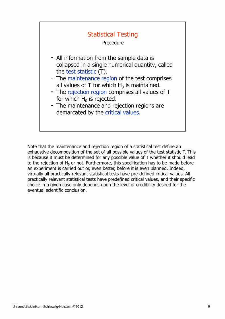
Note that the maintenance and rejection region of a statistical test define an exhaustive decomposition of the set of all possible values of the test statistic T. This is because it must be determined for any possible value of T whether it should lead to the rejection of H0 or not. Furthermore, this specification has to be made before an experiment is carried out or, even better, before it is even planned. Indeed, virtually all practically relevant statistical tests have pre-defined critical values. All practically relevant statistical tests have predefined critical values, and their specific choice in a given case only depends upon the level of credibility desired for the eventual scientific conclusion.


Per se, there is no reason why certain values of T should lead to the rejection of H0

and others do not. However, it is clear that the rejection region must not be totally empty because otherwise, i.e. if H0 is never rejected, a scientific experiment would not make sense in the first place. Furthermore, it is intuitively plausible that T values which are likely to occur if H0 is correct should lead to the maintenance of H0, whereas T values that are unlikely under H0 should lead to its rejection (note that T is of course a random variable itself).


Since it is inherently unknown by the time an experiment is carried out whether H0

or HA is correct, a researcher is faced with the risk of one of two mistakes: erroneously rejecting H0 (type I) or erroneously maintaining H0 (type II).


The standard level of significance used to justify a claim of a statistically significant effect is 0.05. For better or worse, the term 'statistically significant' has become synonymous with α≤0.05. It was Sir Ronald A. Fisher who suggested giving the 5% its special status. In one of his books, he wrote the following about the critical values of a standard normal distribution:

"The value for which α=0.05, or 1 in 20, is 1.96 or nearly 2; it is convenient to take this point as a limit in judging whether a deviation ought to be considered significant or not. Deviations exceeding twice the standard deviation are thus formally regarded as significant." From: RA Fisher (1925) Statistical Methods for Research Workers.

So it was more or less by Fisher's authority that the 5% level of significance has been cast into iron as a criterion for scientific credibility. However, as remarked by statistician Irwin D.J. Bross:

"The continuing usage of the 5% level is indicative of another important practical point: it is a feasible level at which to do research work. […] For suppose that the 0.1% level had been proposed. This level is rarely attainable in biomedical experimentation. If it were made a prerequisite for reporting positive results, there would be very little to report."

As an aside, the definition of the significance level implies that every test with 0.1% significance level is also a test with 5% significance level, but not vice versa.


The position of the critical values depends only upon the distribution of the test statistic T assuming that H0 is correct. In the present example, the rejection region was consequently defined to comprise the most unlikely values of T (i.e. the ones for which the density function yields the smallest values). The probability of observing a T value in the rejection region equals the area under the density curve spanning that region (marked in red), and it appears sensible to define a rejection region comprising probability α/2 at either end of the range of T. The corresponding critical values are labelled cα/2 and c1-α/2 in order to emphasize that, in fact, they are the α/2 and 1-α/2 quantiles of the distribution of T.


The test procedure of choice for comparing the unknown expected value of a normal distribution to a pre-specified reference value µ0 is the one-sample t-test. For the calculation of test statistic T, all it takes are the sample mean (as an estimate of the expected value) and its standard error.

The t-test owes its name to the fact that, under the null hypothesis, T follows a Student t-distribution. It does not follow a standard normal distribution because the standard error of the sample mean is unknown and has to be estimated from the same data. The t-distribution has one parameter, the degrees of freedom, which in the present situation equals the sample size minus 1. With that information, the critical value can be looked up in statistics textbooks.

Please note that the critical values tα/2,n-1 and t1-α/2,n-1 belong to the rejection region of the t-test, not to the maintenance region.


The observed value of the test statistic T is abbreviated by a small letter 't' in order to emphasize that it is the realisation of a random variable. It was calculated in the present example as

Since t exceeds the (right-hand) critical value t0.975,8=2.306 for the t-test, the experiment allows one to conclude that the expected DBP of MI patients differs significantly from 80 mmHg.

.354.29/34.9

|00.8033.87|

n/s

|x|t 0 =−=µ−=


The two error probabilities α and β are intimately linked since both depend upon the location of the maintenance and rejection region of the statistical test in question. If the maintenance region is large, for example, then α will be small and β will be large; if the rejection region is large, the opposite will be true.

The choice of the maintenance region is primarily determined by the fact that the type I error probability must be smaller than the significance level. Within the confines of this requirement, however, a researcher will try to chose the maintenance region such that the type II error probability is minimized, and the power maximized.


The probability β of a type II error depends upon the distribution of T assuming that HA is correct. Usually, this distribution is unknown because it reflects the true but unknown difference between H0 and HA (also called the 'effect' size). Therefore, power considerations in the context of statistical tests usually rely upon speculations on the true effect size.

A type II error occurs if T falls into the maintenance region, so that β equals the area under the density curve of HA spanning the maintenance region (marked in blue).


If µ=80, a type I error occurs each time the observed value of the T statistic falls into the rejection region. Therefore, P80(T≤-2.306, T≥2.306) equals the significance level α of the test.

If µ≠80, however, rejection of the null hypothesis would be tantamount to the avoidance of a type II error. This implies that Pµ(T≤-2.306, T≥2.306)=1-β for all µ≠80.


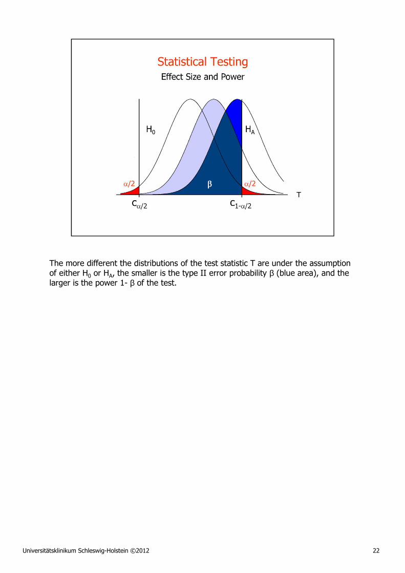
The more different the distributions of the test statistic T are under the assumption of either H0 or HA, the smaller is the type II error probability β (blue area), and the larger is the power 1- β of the test.


Increasing the type I error probability (red area) implies that the maintenance region decreases in size (note that the distance between cα'/2 and c1-α'/2 is smaller than the distance between cα/2 and c1-α/2). Consequently, the type II error probability β (blue area) decreases as well. Similarly, if the type I error probability is reduced, the type II error probability increases.


If it is certain that T values smaller than cα/2, which are undoubtedly unlikely if H0 is correct, are even more unlikely under any imaginable or realistic alternative hypothesis HA, then it would not make sense to include these values in the rejection region.


With one-sided alternative hypotheses, the rejection region is always located on one side of the range of T values, namely the side that includes T values which are likely if the researcher's speculation on the nature of HA is correct.

Since the whole type I error probability is moved to one side in this case, the (single) critical value c1-� is smaller than before. This implies that, under all alternative hypotheses that favour T values "on the correct side of H0", the type II error probability β (blue area) decreases. Therefore, a one-sided test, employing a one-sided hypothesis, generally has more power than a two-sided test, but only if the researcher's speculation on HA is correct.


The gain in power through one-sided tests comes at some cost, namely the prior knowledge about the direction of realistic alternative hypotheses. If this knowledge is not available, a two-sided test must be used to try to disprove the null hypothesis. It is very tempting, but of course not admissible, to carry out an experiment and to perform a one-sided test after the test statistics has been calculated, placing the rejection region on the same side as the actual value of T. This is BCP ("Bad Clinical Practice")! Similarly, it is not enough to just wish that the true effect should be on the chosen side, one has to know it.

Sometimes, two-sided and one-sided alternative hypotheses are also referred to in the scientific literature as 'non-directional' and 'directional', respectively.


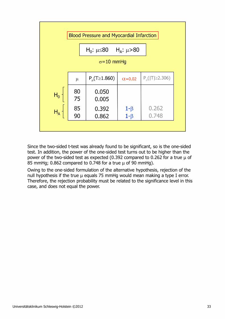
Since the two-sided t-test was already found to be significant, so is the one-sided test. In addition, the power of the one-sided test turns out to be higher than the power of the two-sided test as expected (0.392 compared to 0.262 for a true µ of 85 mmHg; 0.862 compared to 0.748 for a true µ of 90 mmHg).

Owing to the one-sided formulation of the alternative hypothesis, rejection of the null hypothesis if the true µ equals 75 mmHg would mean making a type I error. Therefore, the rejection probability must be related to the significance level in this case, and does not equal the power.


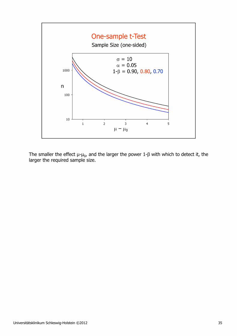
So far, we have assumed that the sample size available for a particular study or experiment is fixed. The researcher is then free to choose the significance level and, by defining the corresponding rejection and maintenance region, the power to detect a particular effect (e.g. a certain difference in expected value) results automatically. In practice, however, sample size calculations are often an important aspect of the study planning. The researcher specifies a "clinically relevant effect" that they want to detect at a given significance level, and then determines the sample size needed to achieve this goal with a particular power (i.e. probability of rejecting H0).

The formulas on the present slide are cheating slightly in that they (i) assume that σis known and (ii) use the quantiles z1-α and z1-β of the standard normal distribution instead of t-quantiles. There are two reasons for this. First, sample size calculations taking the empirical standard deviation into account are difficult. Second, for deciding which t-quantiles to include, the sample size would have to be known beforehand (i.e. a hen and egg situation). This problem can at least approximately be solved by calculating n iteratively, starting with z-quantiles and using t-quantiles thereafter, each time with degrees of freedom corresponding to the sample size calculated in the previous round of iteration.


The smaller the effect µ-µ0, and the larger the power 1-β with which to detect it, the larger the required sample size.


Two-sided tests require slightly larger samples than one-sided tests to detect the same effect with the same power.


In the Pepsi Challenge example, the test statistic T equals the number of probands, out of 100 participants, who preferred Pepsi. This number T contains all information that is required, at least from a statistical point of view, to make a rational decision between the rejection or maintenance of the null hypothesis (i.e. that the probability π of a test person choosing Pepsi equals 50%). Since random variable T has a binomial distribution, the corresponding test is called a "binomial test".

The Pepsi Company would of course wish the test to be performed in one-sided fashion because, in their view, if the two sodas tasted differently at all, then Pepsi would taste better than Coke. In practice, this assumption would rightly be challenged by their competitor. Anyhow, the number of Diet Coke drinkers who preferred Pepsi was not significantly higher than the number of those who did not, even when a one-sided binomial test was applied. Remember that this does not prove the Pepsi Company was wrong. All it means is that the 56:44 ratio did not provide sufficient evidence to reject the null hypothesis at the 5% significance level.


In statistics, there are two major schools of thought on how to design good inference tools: Bayesian and frequentist (or classical). Both schools agree that a scientific experiment usually yields the conditional probabilities of the observed data, given either of the hypotheses involved, i.e. P(D|H0) and P(D|HA). In the Bayesian set-up, however, the prior probabilities of the hypotheses, P(H0) and P(HA), are also assumed to be known. Using Bayes' Theorem, it would then be possible to calculate the posterior probabilities P(H0|D) and P(HA|D) as well, and rational decision making between H0 and HA could be based upon these values.

In many practical situations, however, it may not be reasonable or possible to assign a prior probability to a certain hypothesis. For example, what is the prior probability that a supernova occurs in any particular region of the sky? In such cases, classical hypothesis tests, as developed by Neyman and Pearson and introduced in the present course, provide an inference tool that does not depend upon unrealistic or unsubstantiated assumptions about the prior probabilities of hypotheses. As a downside to this, however, hypothesis tests never yield an answer to questions like "How probable is it that this drug increases blood pressure?".


Fisher obviously agreed that hypothesis tests only allow the rejection or maintenance of hypotheses, but not an assessment of their truth. However, in this verbatim quotation, Fisher also seems to suggest that the scientific credit warranted by the invalidation of a null hypothesis depends upon the extent to which the null hypothesis was actually contradicted by the data. So, it is not surprising that Fisher became the father of the p value.


The one-sided p value is marked in blue whilst the two-sided p value would equal the sum of both the solid and the shaded blue area.

By definition, tobs=c1-p for the one-sided p value and tobs=c1-p/2 for the two-sided p value. The p value therefore equals the significance level at which the null hypothesis would only just be rejected on the basis of the observed value to the test statistic. P values may thus be used for decision making as well, comparing the p value to the significance level α of the test. If p is at most as large as α, then the null hypothesis can be rejected and the result is deemed 'significant'. If p is larger than the significance level, the null hypothesis must be maintained.


In terms of its interpretation, it is appropriate to think of the p value as "[…] an informal index to be used as a measure of discrepancy between the data and the null hypothesis." (Goodman SN, 1999, Ann Intern Med 130: 995-1004). It indicates the strength of evidence for rejecting the null hypothesis H0, rather than simply concluding "reject H0" or "maintain H0". This is why p values are so popular with most scientists and particularly with editors and referees of scientific journals.


In patients with high cholesterol levels, lowering the cholesterol level reduces the risk of coronary events, but the effect of lowering cholesterol levels in the majority of patients with coronary disease, who have average levels, is less clear. In a double-blind trial lasting five years, Sacks and colleagues administered either 40 mg of Pravastatin per day or placebo to approximately 4200 patients with myocardial infarction and normal plasma cholesterol levels.

The authors claimed that the study revealed "... that the benefit of cholesterol-lowering therapy extends to the majority of patients with coronary disease who have average cholesterol levels." However, although the decrease in risk under verum was statistically significant for all major cardiovascular outcomes (i.e. all p values are smaller than 0.05), the question remains whether these risk differences are also clinically significant.


Publication bias arises from the tendency of researchers to publish experimental results that have a positive (i.e. significant) result while not publishing findings where the results are negative (i.e. non-significant) or inconclusive. The effect of this is that published studies may not be truly representative of all valid studies undertaken, and this bias may distort meta-analyses and systematic reviews of large numbers of studies - on which evidence-based medicine increasingly relies. The problem may be particularly serious when the research is sponsored by entities that may have a financial interest in achieving favourable results.

In September 2004, editors of several prominent medical journals (including the New England Journal of Medicine, The Lancet, Annals of Internal Medicine and JAMA) announced that they would no longer publish results of drug research sponsored by pharmaceutical companies unless that research was registered in a public database from the start. In this way, negative results should no longer be able to disappear.

popper's view therefore consists of all hypotheses that ... · hypothesis is correct. one...

Documents