polynomials and interpolation -...
TRANSCRIPT

Polynomials and Interpolation
Selis Oumlnel PhD
SelisOumlnelcopy 2
Effort quotes Success is a ladder you cannot climb with your hands in your
pockets ~American Proverb
Be not afraid of going slowly be afraid only of standing still ~Chinese Proverb
When I was young I observed that nine out of ten things I did were failures So I did ten times more work ~George Bernard Shaw Irish playwright 1856-1950
Opportunity is missed by most people because it is dressed in overalls and looks like work ~Thomas Edison American inventor and businessman 1847-1931
All the so-called secrets of success will not work unless you do ~Author Unknown
SelisOumlnelcopy 3
When do we need datafunction interpolation
Need to obtain estimates of function values at other points
Need to use the closed form representation of the function as the basis for other numerical techniques
SelisOumlnelcopy 4
Goals
Fit a polynomial to values of a function at discrete points to estimate the functional values between the data points
Derive numerical integration schemes by integrating interpolation polynomials ndash Power series ndash Lagrange interpolation forms
Differentiation and integration of interpolation polynomials
Interpolation polynomials using nonequispaced points rarr Chebyshev nodes (roots of the Chebyshev polynomial of the 1st kind)
SelisOumlnelcopy 5
Polynomials
Power series form
y=c1xn+c2x
n-1+hellip+cnx+cn+1
n order of polynomial
ci coefficients
Cluster form
y=((hellip((c1x+c2)x+c3)xhellip+cn)x+cn+1)
Factorized form
y=c1(x-r1)(x-r2)hellip(x-rn)
ri= roots of polynomial
SelisOumlnelcopy 6
Ex Polynomials
Power series form
y=x4+2x3-7x2-8x+12
Cluster form
y=((((x+2)x-7)x-8)x+12)
Factorized form
y= (x-1)(x-2)(x+2)(x+3)
SelisOumlnelcopy 7
Polynomials
A polynomial of order n has n roots
ndash Multiple roots
ndash Complex roots
ndash Real roots
If all ci are real all the complex roots are found in complex conjugate pairs
SelisOumlnelcopy 8
Polynomials in MATLABreg
y=4x4+2x3-7x2+x+7=0 p = [4 2 -7 1 7] roots Finds the roots of a polynomial gtgt p = [4 2 -7 1 7] p = 4 2 -7 1 7 gtgt x=roots(p) x = 093158276438947 + 060071610876714i 093158276438947 - 060071610876714i -118158276438947 + 016770340687492i -118158276438947 - 016770340687492i
SelisOumlnelcopy 9
Polynomials in MATLABreg
y=4x4+2x3-7x2+x+7 poly Determines the coefficients of the original polynomial knowing
the roots The polynomial is normalized to make the leading coefficient 1 gtgt r=[ 093158276438947 + 060071610876714i 093158276438947 - 060071610876714i -118158276438947 + 016770340687492i -118158276438947 - 016770340687492i] gtgt p=poly(r) prsquo ans = 100000000000000 050000000000000 -175000000000000 025000000000000 174999999999999
4 2 -7 1 7
(4)
SelisOumlnelcopy 10
Accuracy of Conversions Conversions may not be accurate due to rounding errors in computations
Coefficients rarr Roots Roots rarr Coefficients
bull Multiple roots Less accurate conversion ldquoComputing a highly multiple root is one of the most difficult problems for
numerical methodsrdquo1
Ex y=(x-5)5 (This equation can be expanded symbolically using simple(y) or
gtgt expand(y) y=x^5-25x^4+250x^3-1250x^2+3125x-3125
gtgt p=sym2poly(y) p = 1 -25 250 -1250 3125 -3125 gtgt roots(p) ans = 500482653710827 + 000350935026218i 500482653710827 - 000350935026218i 499815389493583 + 000567044756022i 499815389493583 - 000567044756022i 499403913591176
SelisOumlnelcopy 11
Accuracy of Conversions
Use the round and real functions to get integer results in taking the roots of polynomials
gtgtround(real(50048+00035i))
ans = 5
gtgt p = [1 -25 250 -1250 3125 -3125]
gtgt r=round(real(roots(p))) r
ans =
5 5 5 5 5
SelisOumlnelcopy 12
Symbolic Calculations
gtgt syms x y z gtgt sym2poly(4x^4+2x^3-7x^2+x+7) ans = 4 2 -7 1 7 gtgt poly2sym([4 2 -7 1 7]) ans = 4x^4+2x^3-7x^2+x+7 gtgt f1=poly2sym([4 2 -7 1 7]sym(t)) f1 = 4t^4+2t^3-7t^2+t+7 gtgt horner(f1) ans = (((4t+2)t-7)t+1)t+7 gtgt f2=x^5-25x^4+250x^3-1250x^2+3125x-3125 gtgt factor(f2) ans = (x-5)^5
SelisOumlnelcopy 13
Symbolic Calculations to Numbers
Symbolic substitution subs(f) replaces all the variables in the symbolic expression f with
values obtained from the calling function or the MATLAB workspace
Ex gtgt f = (x-5)^5 gtgt x=6 gtgt subs(f) ans = 1 gtgt subs(f7) ans = 32 subs(foldnew) replaces old with new in the symbolic expression f gtgt syms a gtgt subs(axa5) ans = 5x
SelisOumlnelcopy 14
Polynomial Calculations in MATLABreg
polyval Evaluates polynomials Ex gtgt syms x gtgt f=4x^4+2x^3-7x^2+x+7 gtgt p=sym2poly(f) p = 4 2 -7 1 7 gtgt x=1 gtgt fx=polyval(px) fx = 7 gtgt fx=polyval(p10) fx = 41317
SelisOumlnelcopy 15
Polynomial Calculations in MATLABreg
polyvalm(px) Evaluates polynomial with matrix argument x must be a square matrix Ex gtgt syms x f=4x^4+2x^3-7x^2+x+7 gtgt p=sym2poly(f) p = 4 2 -7 1 7 gtgt x=[1 10 10 1] gtgt fx=polyvalm(px) fx = 42307 18090 18090 42307 gtgt fx=polyval(px) fx = 7 41317 41317 7
SelisOumlnelcopy 16
Polynomial Calculations in MATLABreg
polyfit Fits polynomial to data p= polyfit(xyn) Finds the coefficients of a polynomial p(x)
best in a least-squares sense n degree of polynomial y data p row vector of length n+1 (polynomial
coefficients In descending powers) A polynomial of order n is determined uniquely if n+1 data
points (xiyi) i=12hellipn+1 are given
SelisOumlnelcopy 17
Ex Polynomial Calculations in MATLABreg Example for using the Polyfit function x=[-24 -08 07 15 36] y=[10 8 5 3 15] figure(1) plot(xy-) grid on xlabel(x) ylabel(y) n=length(x)-1 an=polyfit(xyn) an a3=polyfit(xy3) a3 a2=polyfit(xy2) a2 fitn=poly2sym(an) fitn fit3=poly2sym(a3) fit3 fit2=poly2sym(a2) fit2 figure(2) x1=-3014 plot(xyx1subs(fitnx1)x1subs(fit3x1)x1subs(fit2x1)) xlabel(x) ylabel(y) grid on legend(data pointsn=length(x)-1n=3n=2)
SelisOumlnelcopy 18
Ex Polynomial Calculations in MATLABreg Results of the Polyfit example in the command window an = 30510e-002 36803e-002 -35038e-001 -20526e+000 65885e+000 a3 = 92996e-002 -89465e-002 -22459e+000 63930e+000 a2 = 85356e-002 -16096e+000 59597e+000 fitn =
8793908579215767288230376151711744x^4+5303925840414337144115188075855872x^3-15779610263117394503599627370496x^2-46219723957846832251799813685248x+74180295102719091125899906842624
fit3 = 670104656901501572057594037927936x^3-
644665667751912972057594037927936x^2-50572764820623492251799813685248x+3598950055733773562949953421312
fit2 = 615054214364856172057594037927936x^2-
36244064199638852251799813685248x+67100233400293151125899906842624
SelisOumlnelcopy 19
Ex Polynomial Calculations in MATLABreg
-3 -2 -1 0 1 2 3 41
2
3
4
5
6
7
8
9
10
x
y
-3 -2 -1 0 1 2 3 40
2
4
6
8
10
12
x
y
data points
n=length(x)-1
n=3
n=2
SelisOumlnelcopy 20
Integration of Polynomials
y=c1xn+c2x
n-1+hellip+cnx+cn+1
If the coefficients of the polynomial are given in a row vector p
polyint Integrates the polynomial analytically
polyint(pK) returns a polynomial representing the integral of polynomial p using a scalar constant of integration K
polyint(p) assumes a constant of integration K=0
1 21 21 2
2
1 2
where is an integration constant
n n nn n
n
cc cydx x x x c x c
n n
c
SelisOumlnelcopy 21
Differentiation of Polynomials
y=c1xn+c2x
n-1+hellip+cnx+cn+1
If the coefficients of the polynomial are given in a row
vector p polyder Differentiates the polynomial polyder(p) returns the derivative of the polynomial whose
coefficients are the elements of vector p polyder(AB) returns the derivative of polynomial AB
[QD]=polyder(BA) returns the numerator Q and denominator D of the derivative of the polynomial quotient BA
1 2
1 2( 1) n n
n
dync x n c x c
dx
SelisOumlnelcopy 22
Remember Quotient Rule Quotient rule in calculus is a method of finding the derivative of a
function f(x) that is the quotient of two other functions g(x) and h(x) ie f(x)=g(x)h(x) where h(x)ne0 for which derivatives exist
Ex Let f(x)=(x2-5)(2x3+4x+8) gtgt B=[1 0 -5] A=[2 0 4 8] gtgt [qd]=polyder(BA) q = -2 0 34 16 20
d = 4 0 16 32 16 64 64
2
( ) ( ) ( ) ( ) ( )If ( ) then ( ) ( )
( ) ( )
g x d g x h x g x h x Qf x f x f x
h x dx Dh x
2 3 2 2
3 3 2
( 5) (2 )(2 4 8) ( 5)(6 4)( ) then ( ) ( )
(2 4 8) (2 4 8)
x d x x x x xf x f x f x
x x dx x x
SelisOumlnelcopy 23
Ex Differentiation of Polynomials
gtgt syms x A=x^2+3x+2 B=4x^4+2x^3-x^2+3x+5 gtgt A=sym2poly(A) B=sym2poly(B) A = 1 3 2 B = 4 2 -1 3 5 gtgt polyder(AB) ans = 24 70 52 12 24 21 gtgt poly2sym(polyder(AB)) ans = 24x^5+70x^4+52x^3+12x^2+24x+21 gtgt[QD]=polyder(BA) Q = 8 38 44 6 -14 -9 D = 1 6 13 12 4
SelisOumlnelcopy 24
Product (Convolution) of Polynomials
conv Convolution and polynomial multiplication
C = conv(AB) convolves vectors A and B
The resulting vector is length length(A)+length(B)-1
If A and B are vectors of polynomial coefficients convolving them is equivalent to multiplying the two polynomials
1
1 2 1
Product of two polynomials of order m and order n
gives a polynomial of order d=m+n
d d
c a b d dy y y c x c x c x c
SelisOumlnelcopy 25
Ex Convolution of Polynomials
gtgt PA=[3 5 -1 0] PB=[4 -7 21]
gtgt A=poly2sym(PA)
A = 3x^3+5x^2-x
gtgt B=poly2sym(PB)
B = 4x^2-7x+21
gtgt PC=conv(PAPB)
PC = 12 -1 24 112 -21 0
gtgt C=poly2sym(PC)
C = 12x^5-x^4+24x^3+112x^2-21x
SelisOumlnelcopy 26
Division of Polynomials
deconv Deconvolution and polynomial division [QR] = deconv(AB) deconvolves vector B out of vector A The result is returned in vector Q and the remainder in vector R such that A = conv(BQ) + R If A and B are vectors of polynomial coefficients deconvolution is equivalent to polynomial division The result of dividing A by B is quotient Q and remainder R
a bDivision of a polynomial y by polynomial y satisfies
quotient
remainder upon division
a q b r
q
r
y y y y
y
y
ry
ry
SelisOumlnelcopy 27
Ex Deconvolution of Polynomials
gtgt PA=[3 5 -1 0] PB=[4 -7 21]
gtgt A=poly2sym(PA)
A = 3x^3+5x^2-x
gtgt B=poly2sym(PB)
B = 4x^2-7x+21
gtgt PC=deconv(PAPB)
PC = 075000000000000 256250000000000
gtgt C=poly2sym(PC)
C = 34x+4116
SelisOumlnelcopy 28
Linear Interpolation
It is a line fitted to two data points
Basis for many numerical schemes
ndash Integral of the linear interpolation Trapezoidal Rule
ndash Gradient of the linear interpolation An approximation for the first derivative of the function
Lagrange form
( ) ( ) ( ) or
Newton form
( ) ( )( ) ( ) ( )
b x x ag x f a f b
b a b a
f b f ag x x a f a
b a
y
y=g(x)
f(b)
x
y=f(x)
f(a)
b a
SelisOumlnelcopy 29
Interpolation in MATLABreg interp1 x need to be monotonic Cubic interpolation requires that x
be equispaced interp1 does 1-D interpolation x=[0 1 2 3 4 5] y=[3 5 6 4 2 1] xi=018 g=interp1(xyxilinear) g1=interp1(xyxicubic) g2=interp1(xyxispline) plot(xyrxigbxig1gxig2m) xlabel(x) ylabel(y) legend(y(x)linearcubicspline2)
0 1 2 3 4 5 6 7 80
2
4
6
8
10
12
x
y
y(x)
linear
cubic
spline
SelisOumlnelcopy 30
Interpolation in MATLABreg interp1 Calculate material properties of Carbon Values adapted from S Nakamura 2nd ed p169 T=[300 400 500 600] beta=[3330 2500 2000 1670] alpha=10^4[2128 3605 5324 7190] Ti=[321 440 571] PropertyC=interp1(T[betaalpha]Tilinear) [Ti PropertyC] plot(Talpha-Tbeta-TiPropertyC(1)oTiPropertyC(2)o) legend(alphabetaNew betaNew alpha2) xlabel(Temperature T) ylabel(Thermal expansion beta and diffusivity alpha)
ans = 10e+003 03210 31557 24382 04400 23000 42926 05710 17657 66489
300 350 400 450 500 550 6001000
2000
3000
4000
5000
6000
7000
8000
Temperature T
Therm
al expansio
n
and d
iffu
siv
ity
New
New
SelisOumlnelcopy 31
Polynomial Interpolation with Power Series
1 2 n+1
1 2 n+1
Suppose n+1 data points are given as
x x x
y y y
where
- x are abscissas of data points in increasing order
- the increment between xs is arbitrary
Polynomial of order n passi
1
1 2 1
i i
ng through n+1 data points may be written in power series form as
( )
where c are coefficients
Setting g(x )=y for n+1 data points gives n+1 linear equations ie
Ac=y
To find c
-
n n
ng x c x c x c
Solve Ac=y ie c=Ay OR
- Use polyfit(xyn)
SelisOumlnelcopy 32
Ex Polynomial Interpolation with Power Series Unique solution
Determine the polynomial that passes through 3 data points
(02) (115) (202)
Write the 2nd order polynomial as
g(x)= c1x2+c2x+c3
Setting the polynomial at each data point gives
C1(0)2+c2(0)+c3=2
C1(1)2+c2(1)+c3=15
C1(2)2+c2(2)+c3=02
Solving the above gives
c3=2 c2=-01 c1=-04
ie
g(x)=-04x2-02x+2
gtgt A=[0 0 11 1 1 4 2 1] y=[21502]
gtgt c=Ay crsquo
ans = -04000 -01000 20000
gtgt a=[012] C=polyfit(ay2)
C = -04000 -01000 20000
gtgtC=poly2sym(C) xi=012
gtgt Y=subs(Cxi)
gtgt plot(ayxiY)
0 02 04 06 08 1 12 14 16 18 20
02
04
06
08
1
12
14
16
18
2
SelisOumlnelcopy 33
Lagrange Polynomial Interpolation
The Lagrange form of the equation of a straight line passing through two points
p(x)=(x-x2)y1+(x-x1)y2
(x1-x2) (x2-x1)
The Lagrange form of the parabola passing through three points
p(x)=(x-x2)(x-x3)y1+(x-x1)(x-x3)y2+(x-x1)(x-x2)y3
(x1-x2)(x1-x3) (x2-x1)(x2-x3) (x3-x1)(x3-x2)
SelisOumlnelcopy 34
Ex Lagrange Interpolation Parabola The quadratic (2nd order) polynomial for three
given data points
Substituting into the Lagrange formula gives
p(x)=(x-0)(x-2)4+(x-(-2))(x-2)2+(x-(-2))(x-0)8
(-2-0)(-2-2) (0-(-2))(0-2) (2-(-2))(2-0)
Which simplifies to
p(x)=x(x-2)4 + (x+2)(x-2)2 + x(x+2)8
8 -4 8
= x2+x+2
Ex Adopted from L V Fausett 2nd ed p279
xi yi (i=13)
-2 4
0 2
2 8
-3 -2 -1 0 1 2 30
2
4
6
8
10
12
14
x
y
p(x)=x2+x+2
SelisOumlnelcopy 35
Newton Polynomial Interpolation
The Newton form of the equation of a straight line passing through two points
p(x)=a1+a2(x-x1)
The Newton form of the equation of a parabola passing through three points
p(x)=a1+a2(x-x1)+a3(x-x1)(x-x2)
a1=y1 a2=(y2-y1)(x2-x1) a3=(y3-y2)(x3-x2)-(y2-y1)(x2-x1)
(x3-x1)
SelisOumlnelcopy 36
Ex Newton Interpolation Parabola
The quadratic (2nd order) polynomial for three given data points
Substituting into the Newton formula gives p(x)=a1+a2(x-(-2))+a3(x-(-2))(x-0) Where the coefficients are a1=y1=4 a2=(y2-y1)(x2-x1)=(2-4)(0-(-2))=-1 a3=[(y3-y2)(x3-x2)-(y2-y1)(x2-x1)] =[(8-2)(2-0)-(2-4)(0-(-2))](2-(-2))=1 p(x)=4-(x+2)+x(x+2) = x2+x+2 Ex Adopted from L V Fausett 2nd ed p285
xi yi (i=13)
-2 4
0 2
2 8
-3 -2 -1 0 1 2 30
2
4
6
8
10
12
14
x
y
p(x)=x2+x+2
SelisOumlnelcopy 37
Advantages amp Disadvantages
In many types of problems polynomial interpolation through moderate number of data points works very poorly
Lagrange form
ndash Convenient when the values of x (independent variable) may be the same for different values of the corresponding y
ndash Less convenient than the Newton form when additional data points may be added to the problem
The appropriate degree of the interpolating polynomial is not known
Newton form
ndash Convenient when the spacing between the x data values is constant
ndash More data points can be incorporated and a higher degree polynomial can be generated by making use of the calculations for the lower order polynomial
SelisOumlnelcopy 38
Difficulties of Polynomial Interpolation
Humped and flat data if number of data points is
moderately large
the curve changes shape significantly over the interval
Then there is difficulty with high-order polynomial interpolation
-2 -15 -1 -05 0 05 1 15 2
-04
-02
0
02
04
06
08
1
12
x
y
Shows difficulty with high-order polynomial fit to humped and flat data xi=[-2 -15 -1 -5 0 5 1 15 2] yi=[0 0 0 87 1 87 0 0 0] p=poly2sym(polyfit(xiyi8)) x=-20012 plot(xiyirxsubs(px)) xlabel(x) ylabel(y) grid on
SelisOumlnelcopy 39
0 05 1 15 2 25 3-05
0
05
1
15
2
25
3
x
y
Difficulties of Polynomial Interpolation
Noisy Straight Line if number of data points is
moderately large
Distance between x-values is not even
Then there is difficulty with high-order polynomial interpolation
Shows difficulty with high-order polynomial fit to noisy straight line data xi=[0 2 8 1 12 19 2 21 295 3] yi=[01 22 76 103 118 194 201 208 29 295] p=poly2sym(polyfit(xiyi9)) x=-00013 plot(xiyirxsubs(px)) xlabel(x) ylabel(y) grid on
SelisOumlnelcopy 40
Difficulties of Polynomial Interpolation
Runge function
f(x)=(1+25x2)-1
Using five equally spaced x values
Polynomial interpolation does not give a good approximation
Using more function values at evenly spaced x-values is of no use
There is difficulty with high-order polynomial interpolation
Shows difficulty with high-order polynomial fit to the Runge function xi=[-1 -5 0 5 1] yi=[0385 1379 1 1379 0385] p=poly2sym(polyfit(xiyi4)) x=-10011 f=(1+25x^2)^(-1) plot(xiyirxsubs(px)xfm) xlabel(x) ylabel(y) grid on legend(Data pointsPolynomial fitRunge)
-1 -08 -06 -04 -02 0 02 04 06 08 1-04
-02
0
02
04
06
08
1
x
y
Data points
Polynomial fit
Runge
SelisOumlnelcopy 41
Difficulties of Polynomial Interpolation
Runge function
f(x)=(1+25x2)-1
Using nine equally spaced x values
Interpolation polynomial (of order 8) gives a relatively better approximation compared to polynomial for order 4 but still overshoots the true function
Using more function values at evenly spaced x-values is of no use
There is difficulty with high-order polynomial interpolation
Shows difficulty with high-order polynomial fit to the Runge function xi=[-1 -75 -5 -25 0 25 5 75 1] yi=[039 066 138 39 1 39 138 066 039] p=poly2sym(polyfit(xiyi8)) x=-10011 f=(1+25x^2)^(-1) plot(xiyirxsubs(px)xfm) xlabel(x) ylabel(y) grid on legend(Data pointsPolynomial fitRunge)
-1 -08 -06 -04 -02 0 02 04 06 08 1-15
-1
-05
0
05
1
x
y
Data points
Polynomial fit
Runge
SelisOumlnelcopy 42
Difficulties of Polynomial Interpolation
Runge function
f(x)=(1+25x2)-1
Using better distribution of the data points with more points towards the ends of the interval and fewer in the center
Gives better results
Optimum interpolation (minimizing maximum deviation between the function and the interpolating polynomial) is achieved using zeros of the Chebyshev polynomial as the nodes
Shows difficulty with high-order polynomial fit to the Runge function xi=[-1 -9 -8 -5 0 5 8 9 1] yi=[039 047 059 138 1 138 059 047 039] p=poly2sym(polyfit(xiyi8)) x=-10011 f=(1+25x^2)^(-1) plot(xiyirxsubs(px)xfm) xlabel(x) ylabel(y) grid on legend(Data pointsPolynomial fitRunge)
-1 -08 -06 -04 -02 0 02 04 06 08 10
01
02
03
04
05
06
07
08
09
1
x
y
Data points
Polynomial fit
Runge
SelisOumlnelcopy 43
Chebyshev Polynomials Sturm-Liouville Boundary Value Problem
[p(x)yrsquo]rsquo+[q(x)+λr(x)]y=0 BC1 a1y(a)+a2yrsquo(a)=0 BC2 b1y(b)+b2yrsquo(b)=0
has a special case where
a=-1 b=1 p(x)=(1-x2)12 q(x)=0 r(x )=(1-x2)-12 λ=n2
is called Chebyshevs Differential Equation defined as
(1-x2)yrsquorsquo-xyrsquo+n2y=0 where n is a real number
The solutions of this equation are called Chebyshev Functions of degree n
If n is a non-negative integer ie n=012hellip the Chebyshev Functions are often referred to as Chebyshev Polynomials Tn(x)
Tn(x) form a complete orthogonal set on the interval -1lexle1 wrt r(x)
Using Rodriguesrsquo Formula
For more information httpwwwefundacommathchebyshevindexcfm
122 2
1( ) (1 ) where n=0123
( 1) (2 1)(2 3)1
nn
n n n
x dT x x
n n dx
SelisOumlnelcopy 44
Chebyshev Polynomials
T0(x)=1
T1(x)=x-1
T2(x)=2x2-1
T3(x)=4x3-3x
hellip
Tk(x)=2xTk-1(x)-Tk-2(x)
Ref httpwwwefundacommathchebyshevindexcfm
122 2
1( ) (1 ) where n=0123
( 1) (2 1)(2 3)1
nn
n n n
x dT x x
n n dx
SelisOumlnelcopy 45
Hermite Interpolation
Allows to find a polynomial that matches both the function values and some of the derivative values at specified values of the independent variable
Simplest case function values and first-derivative values are given at each point
Ex Data for the position and velocity of a vehicle at several different times ie
t (time) X (Position) v=dXdt (Velocity)
SelisOumlnelcopy 46
Hermite Interpolation
The cubic Hermite polynomial p(x) has the interpolative properties
p(x0)=y0 p(x1)=y1 prsquo(x0)=d0 prsquo(x1)=d1 Both the function values and their
derivatives are known at the endpoints of the interval [x0x1]
Hermite polynomials were studied by the French Mathematician Charles Hermite (1822-1901) and are referred to as a clamped cubic where clamped refers to the slope at the endpoints being fixed (see figure)
Refhttpmathfullertonedumathewsn2003HermitePolyModhtml
If f[x] is continuous on [x0x1] there exists a unique cubic polynomial
p[x]=ax3+bx2+cx+d such that p[x0]=f[x0] p[x1]=f[x1] prsquo[x0]=frsquo[x0]
prsquo[x1]=frsquo[x1]
SelisOumlnelcopy 47
Hermite Interpolation Summary
ndash Finds a polynomial that agrees with function values and their derivatives at the node points
ndash Uses the Newton form and repeats it for the data points ndash For cubic Hermite polynomial on [01] the basis functions are
ya=-05t3+t2-05t if given f(0)=fb define fa=fc-2sa yb=15t3-25t2+1 f(1)=fc fd=2sb+fb
yc=-15t3+2t2+05t frsquo(0)=sa yd=05t3-05t2 frsquo(1)=sb Then the required interpolating function on [01] is y=faya+fbyb+fcyc+fdyd
Additional Information ndash The cubic Hermite polynomial is a generalization of both the Taylor
polynomial and Lagrange polynomial and it is referred to as an osculating polynomial
ndash Hermite polynomials can be generalized to higher degrees by using more nodes x0 x1hellipxn and extending the agreement at higher derivatives
p(k)[xi]=f(k)[xi] for i=12hellipn and k=12mi
Refhttpmathfullertonedumathewsn2003HermitePolyModhtml
SelisOumlnelcopy 48
Piecewise Polynomial Interpolation
If there are large number of data points
Use piecewise polynomials instead of using a single polynomial (of high degree) to interpolate these points
A spline of degree m is a piecewise polynomial (of degree m) with the maximum possible smoothness at each of the points where the polynomials join
A linear spline is continuous
A quadratic spline has continuous first derivatives
A cubic spline has continuous second derivatives
SelisOumlnelcopy 49
Piecewise Linear Interpolation
Simplest form of piecewise polynomial interpolation
Consider set of four data points
(x1y1) (x2y2) (x3y3) (x4y4) with x1ltx2ltx3ltx4
Defining three subintervals of the x-axis gives
I1=[x1x2] I2=[x2x3] I3=[x3x4]
Subintervals join at the knots which are nodes where the data values are given
SelisOumlnelcopy 50
Piecewise Linear Interpolation Using a straight line on each subinterval the data can be interpolated using a piecewise linear function
A piecewise linear interpolating function is continuous but not smooth at the nodes
2 11 2 1 2
1 2 2 1
3 22 3 2 3
2 3 3 2
343 4 3 4
3 4 4 3
( )
x x x xy y x x x
x x x x
x x x xP x y y x x x
x x x x
x xx xy y x x x
x x x x
SelisOumlnelcopy 51
Ex Piecewise Linear Interpolation
Shows linear piecewise interpolation xi=[ 0 1 2 3] yi=[0 1 4 3] p=poly2sym(polyfit(xiyi3)) x=-10013 yp=subs(px) ylin=interp1(xiyix) plot(xiyirxypxylinm) xlabel(x) ylabel(y) grid on legend(Data pointsPolynomial
fitInterp1 fit)
-1 -05 0 05 1 15 2 25 3-1
0
1
2
3
4
5
6
7
8
xy
Data points
Polynomial fit
Interp1 fit
SelisOumlnelcopy 52
Piecewise Quadratic Interpolation
Using a quadratic equation on each subinterval the functions and their derivatives can be made to agree at the nodes
For n+1 data points there are 2n+n-1 equations ndash n intervals and 3 unknown constant coefficients for each quadratic
polynomial rarr 3n unknowns
ndash 2 equations for each interval (quadratic equations written for each of the end points of the intervals) ie (x1y1) and (x2y2) must satisfy the quadratic equation on the first interval
ndash n-1 points at which the intervals meet where the derivatives of the parabolas on the adjacent intervals are required to be continuous
As a result there are 3n unknowns and 3n-1 equations
There are possible approaches for defining one additional condition
SelisOumlnelcopy 53
Piecewise Quadratic Interpolation
I ldquoKnotsrdquo=ldquoNodesrdquo Approach
Define quadratic functions as
21
i
1
1 i 1 1
1
( ) ( ) ( ) where m is the slope of the function at x2( )
( )(x)= ( ) (x )= ( ) Thus continuity is satisfied
( )
We need to know
i ii i i i i
i i
ii i i i i i i i i
i i
m mS x y m x x x x
x x
x xS m m m S m S x m
x x
11
1
1
211 1 1 1
1
continuity of functions at the nodes In particular at we need
( ) ( ) ( )2( )
Simplifying gives Thus knowing o h 2 t er
i
i ii i i i i i i i i
i i
i ii i i
i i
x x
m mS x y m x x x x y
x x
y ym m m
x x
slopes can be found
SelisOumlnelcopy 54
Ex Piecewise Quadratic Interpolation (knots=nodes)
Data points x=[0 1 2 3] and y=[0 1 4 3]
Set m1=0
m2=2(y2-y1)(x2-x1)-m1=2(1-0)(1-0)-0=2
m3=2(y3-y2)(x3-x2)-m2=2(4-1)(2-1)-2=4
m4=2(y4-y3)(x4-x3)-m3=2(3-4)(3-2)-4=-6 So
In this ldquoknotsrdquo=ldquonodesrdquo approach the choice of slope at x1 (m1=0) influences the overall shape of the curve
21
1
2 2
1
2 2
2
( ) ( ) ( ) for each interval gives2( )
2 0( ) 0 0( 0) ( 0) 0 x 1
2(1 0)
4 2( ) 1 2( 1) ( 1) 1 2( 1) ( 1) 1
2(2 1)
i ii i i i i
i i
m mS x y m x x x x
x x
S x x x x
S x x x x x
2 2
3
x 2
6 4( ) 4 4( 2) ( 2) 4 4( 2) 5( 2) 2 x 3
2(3 2)S x x x x x
SelisOumlnelcopy 55
Piecewise Quadratic Interpolation
II Alternative scheme to the knots=nodes approach
Take the knots as the midpoints between the nodes
(function values are given at the nodes)
For four data points (x1y1) (x2y2) (x3y3) (x4y4)
Define the knots as z1=x1 z2=(x1+x2)2 z3=(x2+x3)2 z4=(x3+x4)2 z5=x4
Spacing between consecutive data points
h1=x2-x1 h2=x3-x2 h3=x4-x3
Then
z2-x1=h12 z3-x2=h22 z4-x3=h32 z2-x2=-h12 z3-x3=-h22 z4-x4=-h32
SelisOumlnelcopy 56
Piecewise Quadratic Interpolation II Alternative scheme to the knots=nodes approach (continued)
Define the quadratic polynomials for each interval as
P1(x)=a1(x-x1)2+b1(x-x1)+c1 x Є [z1z2]
P2(x)=a2(x-x2)2+b2(x-x2)+c2 x Є [z2z3]
P3(x)=a3(x-x3)2+b3(x-x3)+c3 x Є [z3z4]
P4(x)=a4(x-x4)2+b4(x-x4)+c4 x Є [z4z5]
For x=xk rarr Pk(xk)=ck an additional interpolation condition Pk(xk)=yk may be imposed then
ck = yk for k=1234
Imposing continuity conditions on the polynomials at the interior nodes gives 3 equations
P1(z2)=P2(z2) h12a1-h1
2a2+2h1b1+2h1b2=4(y2-y1)
P2(z3)=P3(z3) h22a2-h2
2a3+2h2b2+2h2b3=4(y3-y2)
P3(z4)=P4(z4) h32a3-h3
2a4+2h3b3+2h3b4=4(y4-y3)
SelisOumlnelcopy 57
Piecewise Quadratic Interpolation
II Alternative scheme to the knots=nodes approach (continued)
Imposing continuity conditions on the derivative of the polynomials
Pirsquo(x)=2ai(x-xi)+bi at the interior nodes gives 3 more equations
P1rsquo(z2)=P2rsquo(z2) h1a1+h1a2+b1-b2=0
P2rsquo(z3)=P3rsquo(z3) h2a2+h2a3+b2-b3=0
P3rsquo(z4)=P4rsquo(z4) h3a3+h3a4+b3-b4=0
6 equations and 8 unknown coefficients (a1 a2 a3 a4 b1 b2 b3 b4)
For Pkrsquo(x)=2ak(x-xk)+bk rarr b1 and b4 can be found by imposing
conditions on the derivative values at the interval endpoints x1 and x4
Setting P1rsquo(x1)=0 gives b1=0 and setting P4rsquo(x4)=0 gives b4=0
SelisOumlnelcopy 58
Piecewise Quadratic Interpolation
II Alternative scheme to the knots=nodes approach (continued)
By setting the zero-slope conditions at the interval endpoints for b1=0
and b4=0 the 3 quadratic and 3 derivative equations for the coefficients
become
a1h12 - a2h1
2 + 0 + 0 + 0 + 2b2h1 + 0 + 0 = 4(y2-y1)
0 + a2h22 - a3h2
2 + 0 + 0 + 2b2h2 + 2b3h2 + 0 = 4(y3-y2)
0 + 0 + a3h32 - a4h3
2 + 0 + 0 + b32h3 + 0 = 4(y4-y3)
a1h1 + a2h1 + 0 + 0 + 0 - b2 + 0 + 0 = 0
0 + a2h2 + a3h2 + 0 + 0 + b2 - b3 + 0 = 0
0 + 0 + a3h3 + a4h3 + 0 + 0 + b3 - 0 = 0
SelisOumlnelcopy 59
Ex Piecewise Quadratic Interpolation
Consider data points (00) (11) (24) (33) Set up the linear system of equations using piecewise quadratic interpolation with the knots placed at the midpoints of the data intervals Determine the coefficients of the linear system Write the interpolating piecewise polynomial for each data interval
1
2
3
4
2
3
a1 1 0 0 2 0 4 07429
a0 1 1 0 2 2 12 17714
a0 0 1 1 0 2 4 -33714 c=Ar
1 1 0 0 1 0 0 24571 a
0 1 1 0 1 1 0 25143 b
0 0 1 1 0 1 0 09143 b
A r c
2
1
2
2
2
3
07429 0 x 0005
17714 1 25143 1 1 x 0515
33714 2 09143 2 4
P x x
P x x x
P x x x
2
4
x 1525
24571 3 3 x 2530P x x
SelisOumlnelcopy 60
Ex Piecewise Quadratic (Spline) Interpolation
plotting the quadratic piecewise polynomial solution format short syms x xi=[0123] yi=[0143] A=[1 -1 0 0 2 0 0 1 -1 0 2 2 0 0 1 -1 0 2 1 1 0 0 -1 0 0 1 1 0 1 -1 0 0 1 1 0 1] r=[412-4000] c=Ar since b1=0 and b4=0 c=[c(1) c(2) c(3) c(4) 0 c(5) c(6) 0] n=length(xi) for k=1n if kltn h(k)=(xi(k)+xi(k+1))2end a(k)=c(k) b(k)=c(k+n) C(k)=yi(k) P(k)=c(k)(x-xi(k))^2+b(k)(x-xi(k))+C(k) end h1=[xi(1)01h(1)] h2=[h(1)01h(2)] h3=[h(2)01h(3)] h4=[h(3)01xi(4)] plot(h1subs(P(1)h1)h2subs(P(2)h2)h3hellip subs(P(3)h3)h4subs(P(4)h4)xiyim) legend(P1P2P3P4Data points4) xlabel(x) ylabel(y) grid on 0 05 1 15 2 25 3
0
05
1
15
2
25
3
35
4
45
x
y
P1
P2
P3
P4
Data points
SelisOumlnelcopy 61
Disadvantages of Quadratic Spline Interpolation
Even though better than the ldquonodes=knotsrdquo approach
it requires more computational effort to solve the linear system as the number of data points increase
the coefficient matrix does not have a nice structure (not tridiagonal or banded) which would have reduced the computational effort
SelisOumlnelcopy 62
Ex Piecewise Cubic Hermite Interpolation
This method can be used to preserve monotonicity of x-data MATLABreg built-in function pchip Define an interval xx then the following commands provide in vector yy the values of the interpolant at xx yy = pchip(xyxx) or yy = ppval(pchip(xy)xx) The pchip interpolating function p(x) satisfies On each subinterval x(k) lt= x lt= x(k+1) p(x) is the cubic Hermite interpolant to the given values and certain slopes at the two endpoints Therefore p(x) interpolates y ie p(x(j)) = y(j) and the first derivative prsquo(x) is continuous but prsquorsquo(x) is probably not continuous there may be jumps at x(j) The slopes at x(j) are chosen in such a way that p(x) is shape preserving and respects monotonicity This means that on intervals where the data is monotonic so is p(x) at points where the data have a local extremum so does p(x)
SelisOumlnelcopy 63
Ex Piecewise Cubic Hermite Interpolation and Polyfit Interpolation
Ex for piecewise cubic Hermite interpolation xi=[-3 -2 -1 0 1 2 3] yi=[-8 -1 -8 3 6 65 6] x=[-3013] hermitecoef=pchip(xiyi) yh=ppval(hermitecoefx) polynomialcoef=polyfit(xiyi(length(xi)-1)) yp=polyval(polynomialcoefx) plot(xyhxypxiyim) legend(pchippolyfitData points4) grid on
-3 -2 -1 0 1 2 3-15
-1
-05
0
05
1
pchip
polyfit
Data points
SelisOumlnelcopy 64
Cubic Spline Interpolation (Piecewise Cubic Polynomial)
Better than other methods
Requires continuity of the function as well as its first and second derivatives at each of the ldquoknotsrdquo (boundaries of the subintervals)
For n knots x1ltx2lthellipltxilthellipltxn define n-1 subintervals
I1=[x1x2] hellip Ii=[xixi+1] hellip In-1=[xn-1xn]
Spacing between x values does not need to be uniform so let
hi= xi+1-xi
On Ii=[xixi+1] assume the cubic has the following form
Pi(x) = ai(xi+1-x)3+ai+1(x-xi)3+bi(xi+1-x)+ci(x-xi)
hi hi
Continuity of the second derivative Pirsquorsquo(x) is guaranteed by the form of this function
SelisOumlnelcopy 65
Cubic Spline Interpolation (Piecewise Cubic Polynomial) continued
Pi(x) = ai(xi+1-x)3+ai+1(x-xi)3+bi(xi+1-x)+ci(x-xi)
hi hi
Knowing that at Pi(xi)=yi and Pi(xi+1)=yi+1 bi and ci can be expressed in terms of ai
bi=(yihi)-aihi ci=(yi+1hi)-ai+1hi
Using the condition for continuity of Prsquo(x) at the knots obtain n-2 equations for the n unknowns a1hellipan
For i=1hellipn-2
hiai+2(hi+hi+1)ai+1+hi+1ai+2=(yi+2-yi+1)hi+1 - (yi+1-yi)hi
There are several choices for the conditions on Prsquorsquo(x) at the endpoints which provide the additional conditions (equations) to determine all the unknowns ndash Simplest choice Natural cubic spline assigns Prsquorsquo(x1)=0 and Prsquorsquo(xn)=0 which
makes a1=an=0
SelisOumlnelcopy 66
Cubic Spline Interpolation (Piecewise Cubic Polynomial) continued
Pi(x) = ai(xi+1-x)3+ai+1(x-xi)3+bi(xi+1-x)+ci(x-xi)
hi hi
For n=6 the resulting equations are
2(h1+h2)a2 + h2a3 = (y3-y2)h2-(y2-y1)h1
h2a2 + 2(h2+h3)a3 +h3a4 = (y4-y3)h3-(y3-y2)h2
h3a3 + 2(h3+h4)a4 + h5a5 = (y5-y4)h4-(y4-y3)h3
h4a4 + 2(h4+h5)a5 = (y6-y5)h5-(y5-y4)h4
SelisOumlnelcopy 67
MATLABreg Ex Spline
Shows difficulty with high-order
polynomial fit to the Runge function
syms a
f=(1+25a^2)^(-1)
xi=[-3 -2 -1 0 1 2 3]
yi=subs(fxi)
yp=poly2sym(polyfit(xiyi6))
x=-30013
y=subs(fx)
ys=spline(xiyix)
plot(xiyirxymxsubs(ypx)cxys)
xlabel(x) ylabel(y) grid on
legend(Data pointsRunge functionPolynomial fitSpline fit)
-3 -2 -1 0 1 2 3-04
-02
0
02
04
06
08
1
x
y
Data points
Runge function
Polynomial fit
Spline fit
SelisOumlnelcopy 68
Comparing PCHIP with SPLINE
The function s(x) supplied by SPLINE is constructed in exactly the same way except that the slopes at the x(j) are chosen differently namely to make even srsquorsquo(x) continuous This has the following effects ndash SPLINE is smoother ie srsquorsquo(x) is continuous ndash SPLINE is more accurate if the data are values of a
smooth function ndash PCHIP has no overshoots and less oscillation if the
data are not smooth ndash PCHIP is less expensive to set up ndash The two are equally expensive to evaluate
SelisOumlnelcopy 69
Ex Comparing PCHIP with SPLINE
x = -33 y = [-1 -1 -1 0 1 1 1] t = -3013 plot(xyot[pchip(xyt) spline(xyt)]) legend(datapchipspline4) Ref Example is adopted from MATLABreg Help
-3 -2 -1 0 1 2 3
-1
-08
-06
-04
-02
0
02
04
06
08
1
data
pchip
spline
SelisOumlnelcopy 70
Symbolic Plot ezplot
Ezplot (f) plots the function f(x) over the default domain -2PI lt x lt 2PI
Ezplot(f) plots the implicitly defined function f(xy)=0 over the default domain -2PIltxlt2PI and -2PIltylt2PI
ezplot(f[AB]) plots f(x) over AltxltB and f(xy)=0 over AltxltB and AltyltB
Using a string to express the function gtgt ezplot(x^2 - 2x + 1) Using a function handle (in case there are other
parameters k in the function) function for ezplot function z = funplot(xyk) z = x^k - y^k - 1 gtgt for k= 110 ezplot((xy)funplot(xyk)) end
-6 -4 -2 0 2 4 6
0
10
20
30
40
50
x
x2 - 2 x + 1
-6 -4 -2 0 2 4 6
-6
-4
-2
0
2
4
6
x
y
funplot(xy2) = 0
SelisOumlnelcopy 71
Other Web Sources of Information
httpplanetmathorgencyclopediaLectureNotesOnPolynomialInterpolationhtml
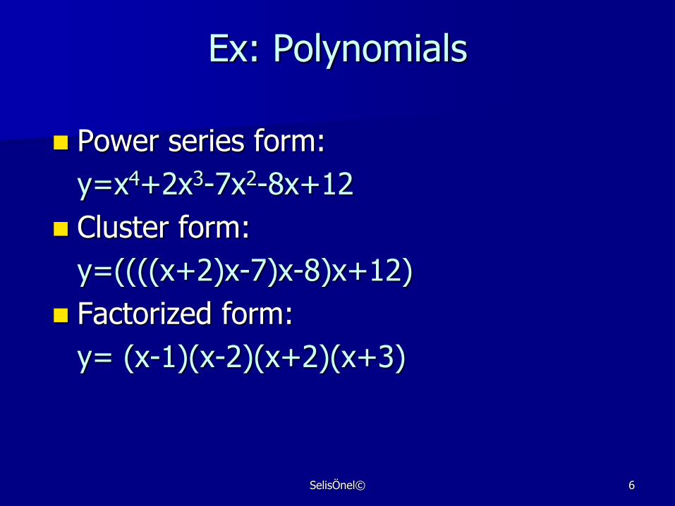
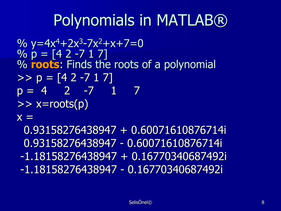
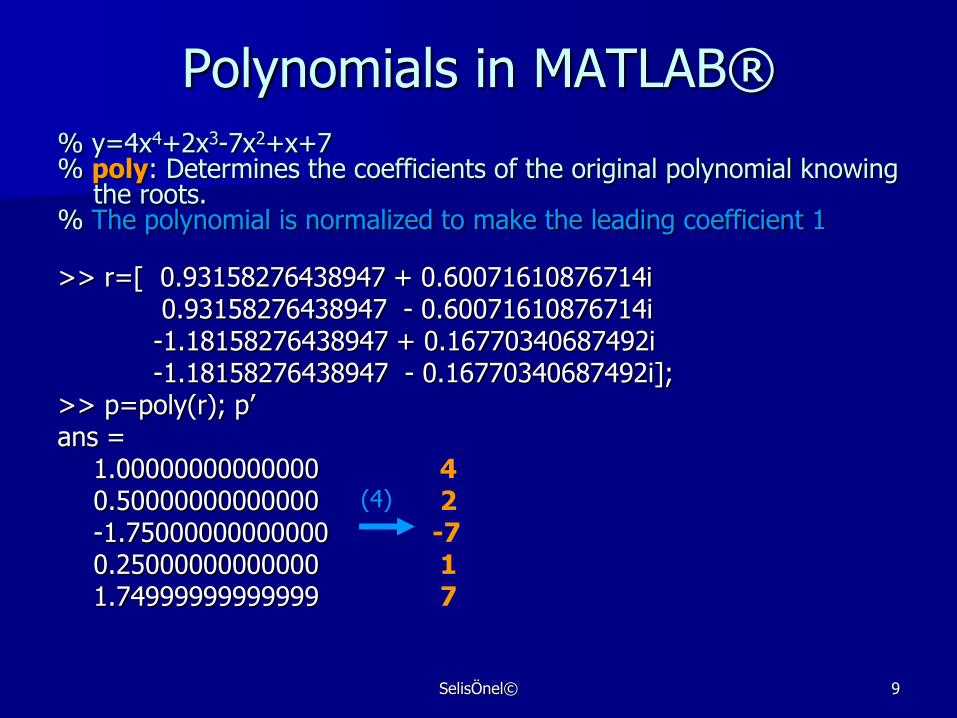
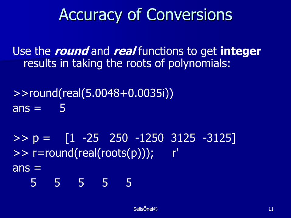
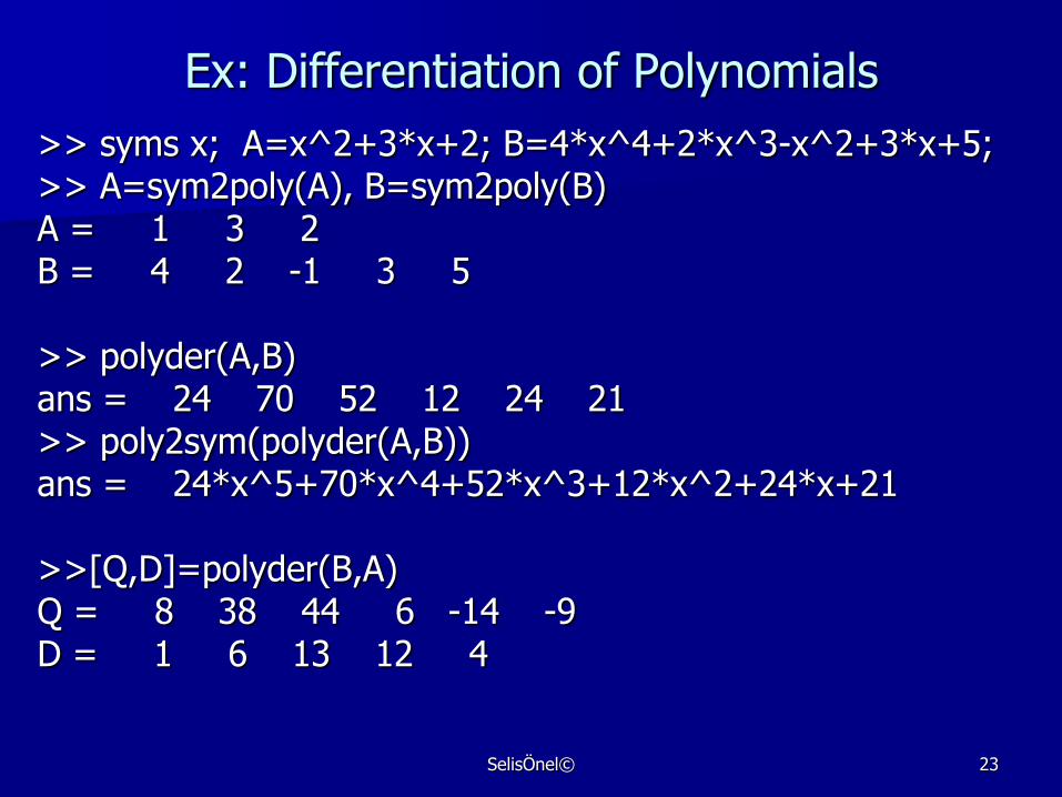
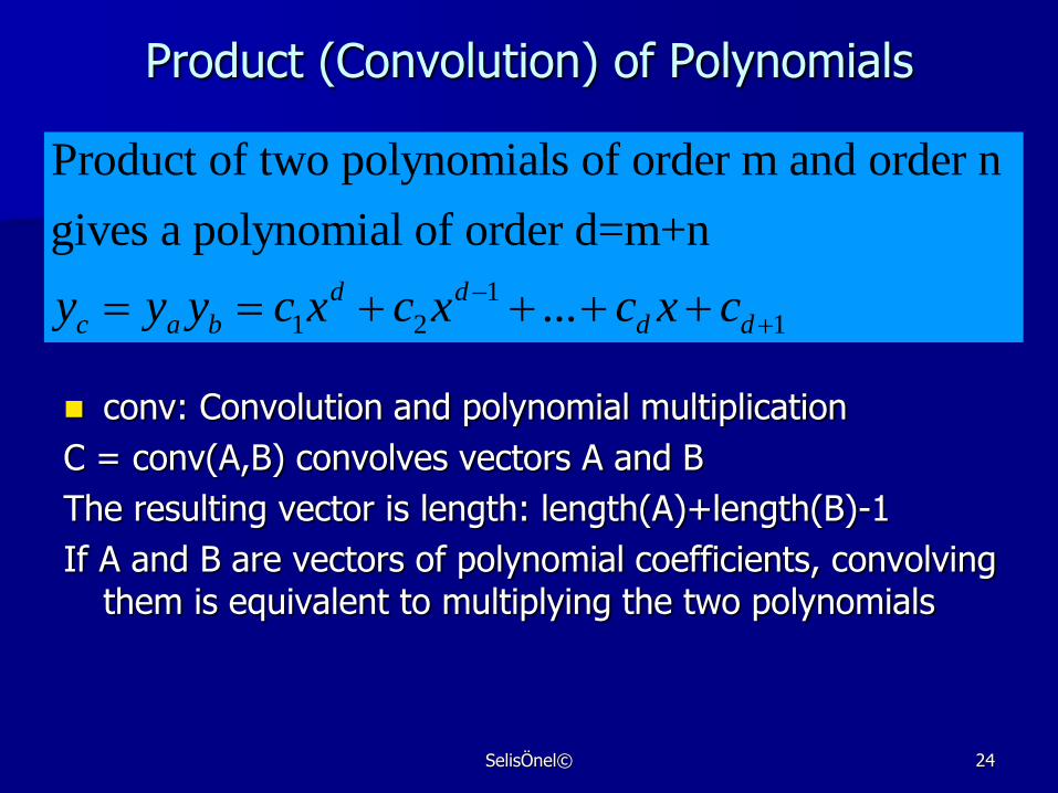
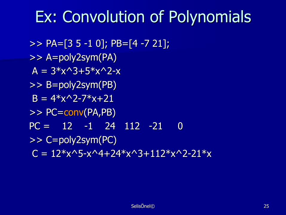
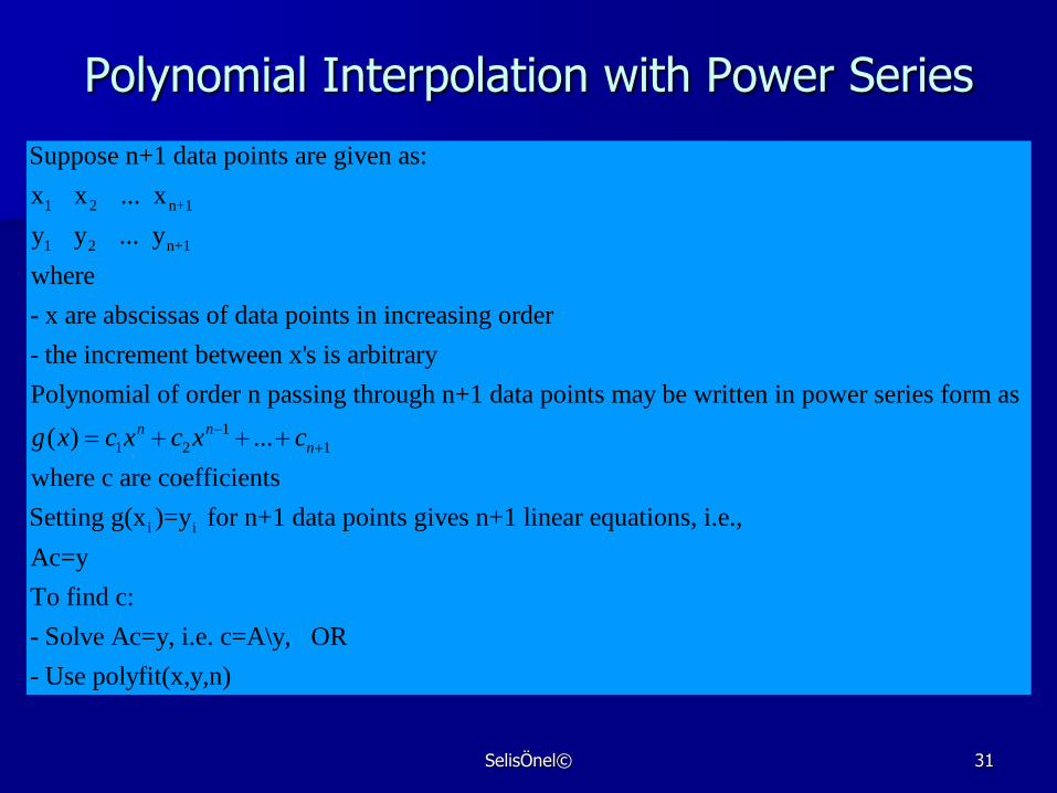
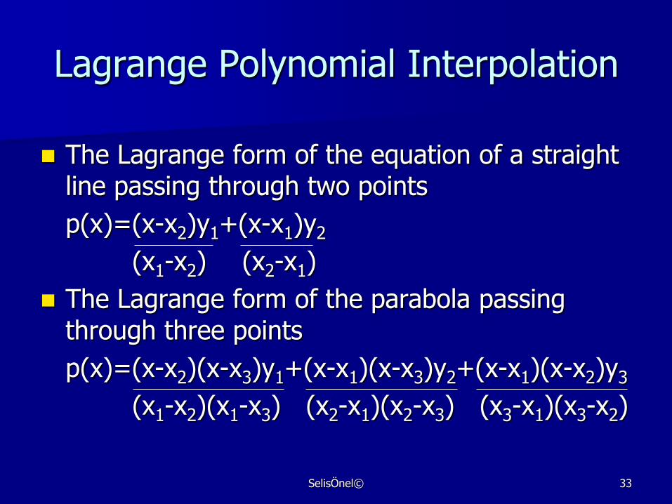
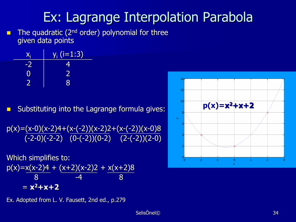
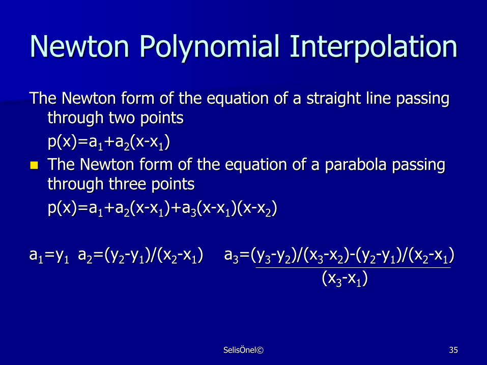
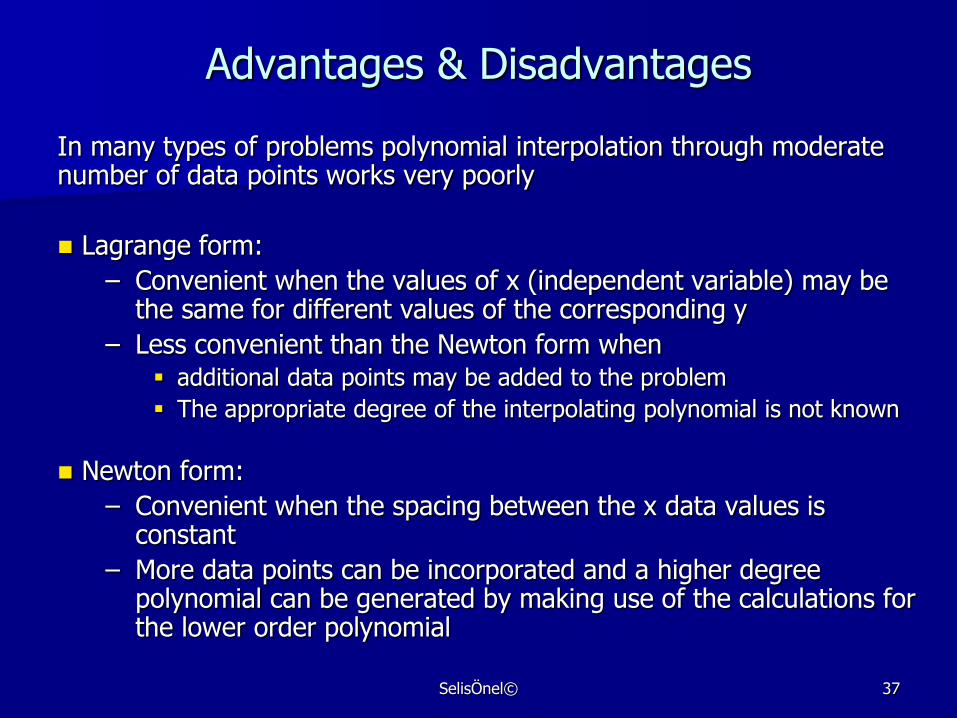
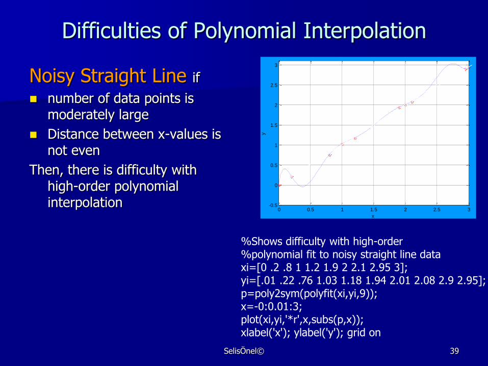
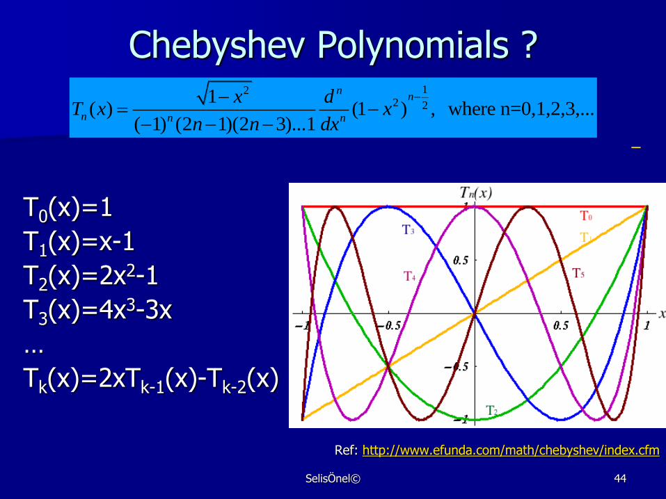
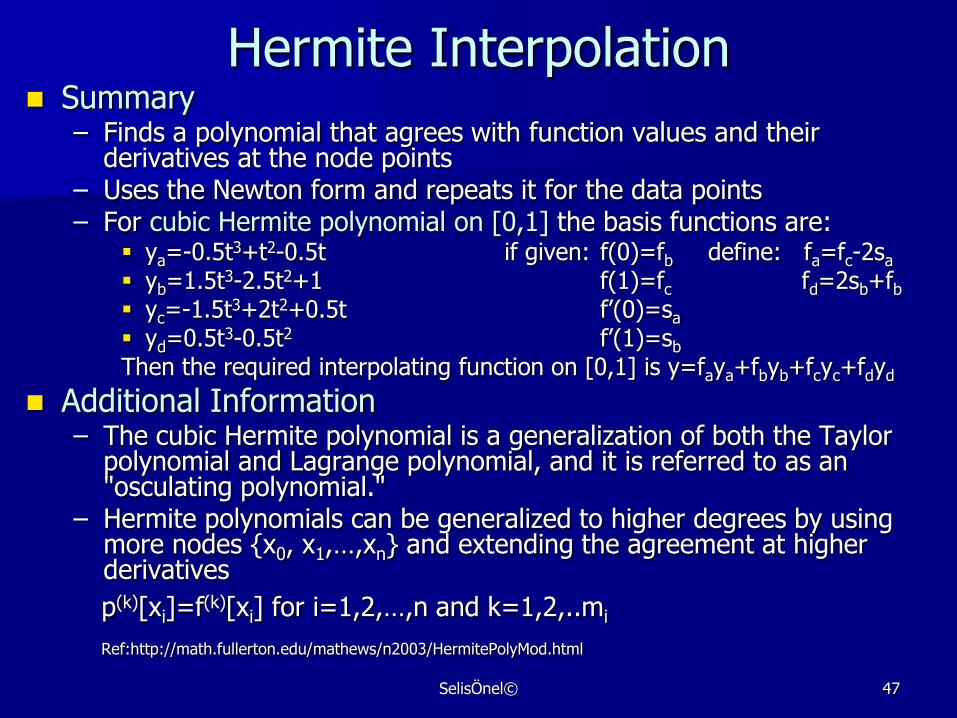
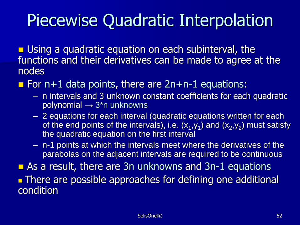
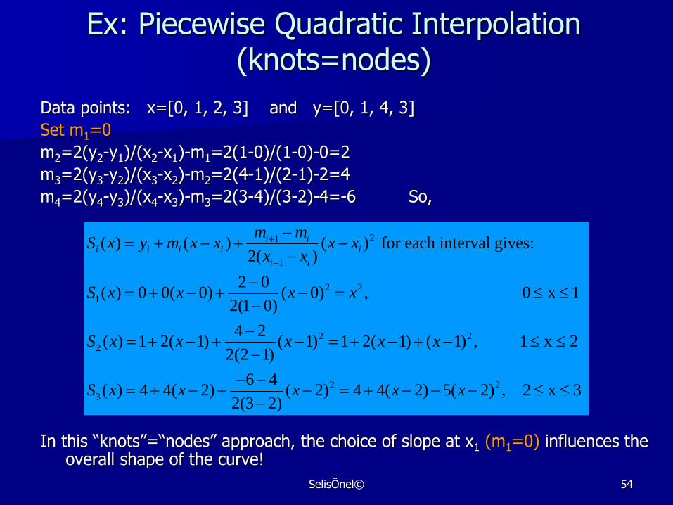
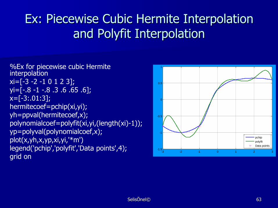
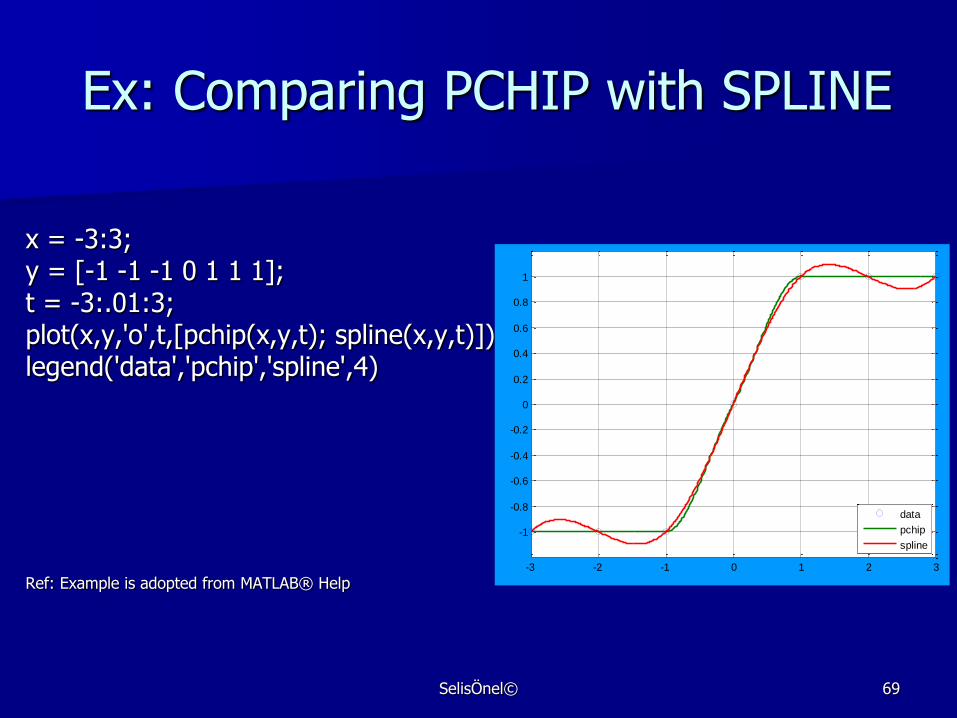

SelisOumlnelcopy 71
Other Web Sources of Information
httpplanetmathorgencyclopediaLectureNotesOnPolynomialInterpolationhtml