polyfolds and fredholm theory part 1 - uni-leipzig.deschwarz/sft/manuscripthwz... · 2008-09-30 ·...
TRANSCRIPT

Polyfolds and Fredholm Theory
Part 1
May 11, 2005
Preliminary Version *
Helmut Hofer
Kris Wysocki
Eduard Zehnder
Courant Institute, New York University, New York,
New York
E-mail address: [email protected]
Department of Mathematics and Statistics, University
of Melbourne, Melbourne, Australia
E-mail address: [email protected]
Department of Mathematics, ETH-Zurich, Switzerland
E-mail address: [email protected]
*Copyright@2005 by Hofer, Wysocki and Zehnder


Contents
Introduction 7
Chapter 1. SC-Calculus in Banach Spaces 131.1. sc-Smooth Spaces 131.2. sc-Smooth Maps 151.3. sc-Operators 261.4. sc-Manifolds 301.5. A Space of Curves 321.6. Appendix I 43
Chapter 2. M-Polyfolds 492.1. Cones and Splicings 492.2. Example of a Splicing 522.3. Smooth maps between splicing cores 592.4. M-Polyfolds 622.5. Corners and Boundary points 662.6. Appendix II 70
Chapter 3. The space of curves as an M-Polyfold 793.1. The Topology on X 793.2. M-Polyfold Charts on X 883.3. The level-k curves as an M-Polyfold 107
Chapter 4. M-Polyfold Bundles 1254.1. Local Strong sc-Bundles 1254.2. Strong sc-Vector Bundles 1274.3. Example of a Strong Bundle over X(a, b) 1294.4. Strong M-Polyfold Bundles 130
Chapter 5. Local sc-Fredholm Theory 1335.1. An Infinitesimal sc-Implicit Function Theorem 1335.2. sc-Fredholm Germs and Perturbations 1395.3. Fillers and Local M-Polyfold Fredholm Germs 1435.4. Local solutions of polyfolds Fredholm germs 146
Chapter 6. Global sc-Fredholm Theory 163
5

6 CONTENTS
6.1. Fredholm sections 1636.2. Mixed convergence and auxiliary norms 1646.3. Proper Fredholm Sections 1686.4. Transversality and Solution Set 1706.5. Perturbations 1716.6. An Example of a Fredholm Operator 172
Chapter 7. Fredholm Theory in Polyfold Groupoids 1817.1. Fred-Submersions 1817.2. Polyfold Groupoids 1867.3. Fractions of Equivalences 1927.4. Strong Bundles over Polyfold Groupoids 1967.5. Proper Etale Polyfold Groupoids 1977.6. Ep-Polyfolds 2027.7. Fredholm Multi-Sections 2037.8. Transversality and Perturbations 208
Bibliography 211
Index 213

INTRODUCTION 7
Introduction
This book is the first in a series of four books devoted to a gen-eral nonlinear Fredholm theory on spaces of varying dimensions. Theusefulness of this theory will be illustrated by a variety of applica-tions including Morse homology, Gromov-Witten theory, Floer theoryand Symplectic Field theory. We believe that there are many otherpossible applications to nonlinear PDE-problems beyond what we de-scribe here. From a very abstract point of view the above mentionedproblems are very similar. To explain this point we recall some facts.Gromov-Witten theory, Floer theory, Contact homology, or more gen-erally Symplectic Field theory are all based on the study of compactifiedmoduli spaces, or even infinite families of such spaces interacting witheach other. The data of these moduli spaces are encoded in convenientways leading for example to so-called generating functions in Gromov-Witten theory or to Floer-Homology in the Floer-Theory. Commonfeatures include the following.
• The moduli spaces are solutions of elliptic PDE’s showing dra-matic non-compactness phenomena having well-known nameslike “bubbling-off”, “stretching the neck”, “blow-up”, “break-ing of trajectories”. These descriptions are a manifestation ofthe fact that from classical analytical viewpoint one is con-fronted with limiting phenomena, where classical analyticaldescriptions break down.
• When the moduli spaces are not compact, they admit non-trivial compactifications like the Gromov compactification ofthe space of pseudoholomorphic curves or the space of brokentrajectories in Morse theory.
• In many problems like in Floer theory, Contact homology orSymplectic Field theory the algebraic structures of interest areprecisely those created by the “violent analytical behavior”and its “taming” by suitable compactifications. In fact, thealgebra is created by the complicated interactions of manydifferent moduli spaces.
In our books, we will propose a general functional analytic approachwhich allows us, in particular, to understand the elliptic problems aris-ing in symplectic geometry. Also here the lack of compactness does notpermit a satisfactory classical description. On the other hand, the lackof compactness is precisely the source of interesting invariants. Thisis our motivation for introducing the new framework. The frameworkshould fit into the following general scheme for producing invariantsfor geometric problems. Starting with a concrete problem, we have a

8 CONTENTS
distinguished set G of geometric data. The choice of τ ∈ G leads toa nonlinear elliptic differential operator Lτ . We are interested in thesolution set M of Lτ = 0. We want to extract invariants from this so-lution set which are independent of the actual choice τ . In interestingcases the solution sets are not compact. The first task is then to
1) find a good compactification M of the solution set M.This task can be very difficult, as the compactification of the space
of pseudoholomorphic curves in symplectic cobordisms in [3] shows.However, our abstract theory will give quite a number of ideas how toconstruct compactifications in concrete case.
2) Next we construct a bundle Y → X so that L becomesa section whose zero-set is M and not only M.
Clearly, if the bundle Y → X would not have some additional “goodproperties”, this formulation would be quite useless. What are thesegood properties? Taking classical (nonlinear) Fredholm theory as aguide, we would like our spaces to have tangents and we would liketo be able to linearize problems. Information about the linearizationshould then allow us to design implicit function theorems. In addi-tion, we would like to have a notion of transversality and an abstractperturbation theory which would permit to perturb a section into ageneral position. Finally, in case of transversality, the solution set{L = 0} should be a smooth manifold or a smooth orbifold ina natural way. How does classical Fredholm theory achieve this? Inthe classical theory the ambient space X is a smooth Banach man-ifold and Y is a smooth Banach space bundle over it. Then L is asmooth section and its linearization at zero is Fredholm. The usualimplicit function theorem then describes the solution set provided thelinearization is surjective. The smooth structure on the solution setis induced from the smooth structure of the ambient space. In fact,in case of transversality the solutions set is a smooth submanifold. Itshould be emphasized that the classical theory has a lot of luxury buildin. If one ultimately is only interested in obtaining a smooth structureon the solution space (in case of transversality), then one expects tobe able to give up quite a lot of structure on the ambient space X. Inour case we want the compactified solution set to be contained in theambient space X, and an analysis of concrete examples reveals thatthere cannot be a structure for which X is locally homeomorphic to anopen set in a Banach space. In fact, one needs models admitting locallyvarying dimensions in order to deal with phenomena like bubbling-off.At first sight, it seems rather doubtful whether such objects could everhave tangent spaces. Moreover, for any useful concept of smoothness

INTRODUCTION 9
in our new theory, the concrete examples listed above indicate that theshift-map
R × L2(R) → L2(R) : (t, u) → u(· + t)
should be smooth (in a new sense yet do be defined). This map is justbarely continuous in the classical sense. Surprisingly there is a way ofovercoming this problem. One can generalize calculus by introducinga new concept of smoothness. This then allows us to define new localmodels for spaces which still admit tangent spaces and which replacethe open sets in Banach spaces. Moreover, the classical smoothnessof transition maps can be replaced by the new concept of smoothness.Our local models now have varying dimensions. The spaces obtainedthis way are called polyfolds and their bundles are called polyfoldbundles. As it turns out, on these polyfold bundles can be developed aFredholm theory which satisfies all our requirements. Roughly a sectionis a Fredholm section if in suitable local coordinates it has a suitablenormal form. Our notion of a chart is very weak because the concept ofsmoothness is relaxed. As a consequence, we obtain more flexibility inbringing problems into a normal form. In other words, more problemsthan before turn out to be nonlinear Fredholm problems.
Finally, we want to make more precise what it means that manyFredholm problems interact with each other. Let us explain somebackground. The compactifications of the solution spaces which oneintroduces are usually composed of ingredients which are solutions ofPDE’s obtained from the original PDE’s as limit cases. They are usu-ally Fredholm problems. If we take the disjoint union of all theseFredholm problems, we obtain a new Fredholm problem having thefollowing structure. We find a Fredholm section f of a polyfold bun-dle Y → X. The polyfold X will have a “boundary with corners”,a notion to be defined. Polyfolds are, in particular, second countableparacompact spaces. As it will turn out, there is a function d : X → N,called the degeneracy function, so that every point x ∈ X has an openneighborhood U(x) satisfying d|U(x) ≤ d(x). Now the boundary ∂Xis by definition the subset of X consisting of points having degeneracyd(x) ≥ 1. Consider the connected components in {x ∈ X | d(x) = 1}.The closure of such a connected component will be called a face. Everypoint x ∈ ∂X lies in the intersection of at most d(x) faces. There isa rich structure if we know a priori that every point lies in preciselyd(x)-many faces. This will be the case in all our applications. Nowwe are able to formalize what it means that Fredholm problems areinteracting with each other. We describe only a particular case of ourmore general theory. There is a countable set S (equipped with the
10 CONTENTS
discrete topology) and a subset D of S ×X ×X which is the union ofconnected components in X ×X and a smooth map ◦ : D → X whoseimage is ∂X and which meets certain axioms. This map extends to amap S×Y ×Y → Y as a fiber-wise linear isomorphism. The Fredholmsection f : X → Y is compatible with the operation ◦, if
f(◦(s, x, x′)) = ◦(s, f(x), f(x′)).
The interpretation is as follows. Given two points x and x′ in X andthe “recipe” s in S, we can construct a new element ◦(s, x, x′). If, forexample, x and x′ are solutions of the Fredholm problem then ◦(s, x, x′)is also a solution. This way we can explain the boundary ∂X in termsof X via the operation ◦. The above structure (f : X → Y, ◦) is calleda Fredholm problem with operation. As it turns out Morse homology,Floer theory, Contact homology and Symplectic Field theory can beunderstood as Fredholm problems with operations. Hence the thirdstep in a concrete problem is
3) identify the operation.We shall develop a theory of cobordisms between Fredholm prob-
lems with operations and some interesting algebra to describe suchproblems.
The four volumes are organized in the following way,Volume I. In the first part of the current volume, we introduce
the new calculus and develop the functional analysis and differentialgeometry needed in order to construct our new spaces. Let us remindthe reader that most of the constructions in differential geometry arefunctorial. Hence if we introduce new spaces as local models which havesome kind of tangent spaces, and if we can define smooth maps betweenthese spaces and their tangent maps, then the validity of the chainrule allows us to carry out most differential geometric constructionsprovided we have smooth (in the new sense) partitions of unity. Usingthe new local models for spaces we construct the M polyfolds. Onthese new spaces, we develop a nonlinear Fredholm theory and proveseveral variants of the implicit function theorem. All the conceptsare illustrated by an application to classical Morse theory. Let us,however, note the following. Having the notion of an M-polyfold we cangeneralize the notion of a Lie-groupoid and define polyfolds by copyingthe groupoid approach to orbifolds. This is straightforward and allowsus, with some of the results in volume II, to develop the Gromov-Wittentheory, where in case of transversality the moduli spaces have naturalsmooth (in the classical sense) structures.

INTRODUCTION 11
Volume II. In this volume, we construct a polyfold set-up forSymplectic Field theory. As a by-product, we obtain a polyfold set-upfor Gromov-Witten theory. We show that there are natural polyfoldsand polyfold bundles over them so that the Cauchy-Riemann operatoris a Fredholm section in our new sense. The zero set is the union of allcompactified moduli spaces. Polyfolds are the orbifold generalisationof M-polyfolds and have descriptions in terms of a theory of polyfold-groupoids, where the notion of manifold is replaced by that of an M-polyfold.
Volume III. Here we develop the Fredholm theory in polyfoldswith operations. It will be illustrated by several applications. Theeasiest and very instructive application is again Morse theory. Anotherapplication is the Contact homology.
Volume IV: This volume is entirely devoted to Symplectic Fieldtheory, which is obtained as an application of a theory which one mightcall Fredholm theory in polyfold groupoids.
The tentative titles of the books are:
“Fredholm Theory in Polyfolds I: Functional Analytic Meth-ods”;“Fredholm Theory in Polyfolds II: The Polyfolds in SymplecticField Theory”;“Fredholm Theory in Polyfolds III: Operations”;“Fredholm Theory in Polyfolds IV: Applications to SymplecticField Theory”.


CHAPTER 1
SC-Calculus in Banach Spaces
In order to develop the generalized nonlinear Fredholm theory neededfor the symplectic field theory we start with some calculus issues. Inthe following “sc” stands for ”scale” as well as for ”scale compact” andthe meaning will become clear in the definition below.
1.1. sc-Smooth Spaces
We begin by introducing the notion of an sc-smooth structure on aBanach space and on its open subsets.
Definition 1.1. Let E be a Banach space. An sc-smooth struc-ture on E is given by a nested sequence
E = E0 ⊇ E1 ⊇ E2 ⊇ · · · ⊇⋂m≥0
Em = E∞
of Banach spaces Em, m ∈ N = {0, 1, 2, · · · }, having the followingproperties.
• If m < n, the inclusion En ↪→ Em is a compact operator.
• The vector space E∞ defined by
E∞ =⋂m≥0
Em
is dense in Em for every m ≥ 0.
It follows, in particular, that En ⊆ Em is dense and the embeddingis continuous if m < n. We note that E∞ has the structure of a Frechetspace. If U ⊂ E is an open subset we define the induced sc-smoothstructure on U to be the nested sequence Um = U ∩ Em. Given ansc-smooth structure on U we observe that Um inherits the sc-smoothstructure defined by (Um)k = Um+k. In the following most of the timethere is no possibility of confusing the Banach space Em with the sc-Banach space Em. In case where is an ambiguity we will write Em toemphasize that we are dealing with the Banach space with sc-structure(Em+i)i≥0. Similarly we will distinguish between Um and Um.
13

14 1. SC-CALCULUS IN BANACH SPACES
Here is an example.
Example 1.2. Consider E = L2(R). Take a strictly increasingsequence of real numbers δ0 = 0 < δ1 < δ2 · · · starting at 0. Thendefine the space Em = Hm,δm to consist of all L2-functions u whoseweak derivatives Dku up to order m belong to L2 if weighted by eδm|s|,i.e.,
eδm|·|Dku ∈ L2(R) for all k ≤ m.
The space Em is equipped with the inner product
(u, v)m =∑
0≤k≤m
(eδm|s|Dku, eδm|s|Dkv).
Using the appropriate compact Sobolev embedding theorem on boundeddomains and the strictly increasing weights at the infinities one estab-lishes the compactness of the inclusion operators En ↪→ Em for n > m.Clearly, the images are dense. Armed with this example the readershould make a similar construction for functions defined on R × S1.Such maps will be important in SFT.
Given E and F with sc-smooth structures then the Banach spaceE⊕F carries the sc-smooth structure defined by (E⊕F )m = Em⊕Fm.
Definition 1.3. Let U and V be open subsets of sc-smooth Banachspaces. A continuous map ϕ : U → V is said to be of class sc0
or simply sc0 if it induces continuous maps on every level, i.e., theinduced maps
ϕ : Um → Vm
are all continuous.
We illustrate the concept by the following example.
Example 1.4. Take the space E from Example 1.2 equipped withthe sc-structure given there. Define the R-action of translation
(1.1) Φ : R ⊕ E → E, (t, u) �→ t ∗ u by
(t ∗ u)(s) = u(s + t).
It is not difficult to prove that the map (t, u) �→ t ∗u is of class sc0, seeLemma 1.39 below.
Next we define the tangent bundle.

1.2. SC-SMOOTH MAPS 15
Definition 1.5. Let U be an open subset in a sc-smooth Banachspace E equipped with the induced sc-smooth structure. Then the tan-gent bundle of U is defined by TU = U1 ⊕ E with the inducedsc-smooth structure defined by the nested sequence
(TU)m = (U1 ⊕ E)m = Um+1 ⊕ Em
together with the sc0-projection
p : TU → U1.
Note that the tangent bundle is not defined on U but merely on thesmaller subset U1 of level 1. For instance, in Example 1.2 the tangentbundle of E is given by
TE = H1,δ1 ⊕ L2
with the sc-smooth structure (TE)m = H1+m,δm+1 ⊕ Hm,δm.
1.2. sc-Smooth Maps
Next we introduce the notion of a sc1-map. Let us first recall thata map f : U → V between open subsets of Banach spaces E and Fis differentiable at the point x ∈ U if there exists a bounded linearoperator L : E → F satisfying
1
‖h‖E‖f(x + h) − f(x) − Lh‖F → 0 as ‖h‖E → 0.
The operator L is then called the derivative of f at x and is denotedby df(x). The map is of class C1 if it is differentiable at every x ∈ Uand if the map U → L(E, F ), x → df(x) is continuous. Here L(E, F )is the space of bounded linear operators equipped with the norm
‖L‖L(E,F ) = sup{h∈E| ‖h‖E≤1}
‖Lh‖F .
If E is infinite-dimensional, then the requirement that the map
U → L(E, F ), x → df(x)
is continuous is much stronger than the requirement that the map
U ⊕ E → F, (x, h) → df(x)h
is continuous. The latter merely implies that
U → Lco(E, F )
is continuous, where Lco(E, F ) stands for L(E, F ) equipped, however,with the compact open topology which is not a normable topology ifdim(E) = ∞ but merely a locally convex topology.

16 1. SC-CALCULUS IN BANACH SPACES
Definition 1.6. Let E and F be sc-smooth Banach spaces and letU ⊂ E be an open subset. An sc0-map f : U → F is said to be sc1 orof class sc1 if the following conditions hold true.
(1) For every x ∈ U1 there exists a linear map Df(x) ∈ L(E0, F0)satisfying for h ∈ E1
1
‖h‖1‖f(x + h) − f(x) − Df(x)h‖0 → 0 as ‖h‖1 → 0.
(2) The tangent map Tf : TU → TF defined by
Tf(x, h) = (f(x), Df(x)h)
is an sc0-map.
The linear map Df(x) will in the following often be called thelinearization of f at the point x.
The second condition requires that Tf : (TU)m → (TF )m is con-tinuous for every m ≥ 0. In detail, the map
Um+1 ⊕ Em → Fm+1 ⊕ Fm
(x, h) �→ (f(x), Df(x)h)
is continuous for every m ≥ 0. It follows, in particular, that
(1.2) Df(x) ∈ L(Em, Fm)
if x ∈ Um+1, for every m ≥ 0.
Fm+1 −−−→ Fm −−−→ Fm−1�⏐⏐f
�⏐⏐f
�⏐⏐f
Um+1 −−−→ Um −−−→ Um−1
Fm+1 −−−→ Fm −−−→ Fm−1�⏐⏐Df(x)
�⏐⏐Df(x)
�⏐⏐Df(x)
Em+1 −−−→ Em −−−→ Em−1
From the first condition in Definition 1.6 it follows that f : U1 → F0
is differentiable and the derivative df(x) at x ∈ U1 is given by
df(x) = Df(x) ∈ L(E1, F0).
Actually, we shall show that f ∈ C1(U1, F ). This is a consequence ofthe following alternative definition of a class sc1-map.
Proposition 1.7 (Alternative definition). Let E and F be sc-smooth Banach spaces and let U ⊂ E be an open subset. An sc0-map

1.2. SC-SMOOTH MAPS 17
f : U → F is of class sc1 if and only if the following conditions holdtrue.
(1) For every m ≥ 1, the induced map
f : Um → Fm−1
is of class C1. In particular, the derivative df is the continuousmap
Um → L(Em, Fm−1), x → df(x).
(2) For every m ≥ 1 and every x ∈ Um the continuous linearoperator df(x) : Em → Fm−1 has an extension to a continuouslinear operator Df(x) : Em−1 → Fm−1. In addition, the map
Um ⊕ Em−1 → Fm−1
(x, h) → Df(x)h
is continuous.
Proof. Assume that f : U → F is of class sc1 according to Def-inition 1.6. Then f : U1 → F is differentiable at every point x withthe derivative df(x) = Df(x)|E1 ∈ L(E1, F ), so that the extensionof df(x) : E1 → F to a continuous linear map E → F is the postu-lated map Df(x). We claim that the derivative x �→ df(x) from U1 intoL(E1, F ) is continuous. Arguing indirectly we find ε > 0 and sequencesxn → x in U1 and hn of unit norm in E1 satisfying
(1.3) ‖df(xn)hn − df(x)hn‖0 ≥ ε.
Taking a subsequence we may assume, in view of the compactness ofthe embedding E1 ↪→ E0, that hn → h in E0. Hence, by the continuityproperty (2) in Definition 1.6, df(xn)hn = Df(xn)hn → Df(x)h in F0.Consequently,
df(xn)hn − df(x)hn = Df(xn)hn − Df(x)hn → Df(x)h − Df(x)h = 0
in F0, in contradiction to (1.3).Next we prove that f : Um+1 → Fm is differentiable at x ∈ Um+1
with derivative
df(x) = Df(x)|Em+1 ∈ L(Em+1, Fm)
so that the required extension of df(x) is the operator Df(x) ∈ L(Em, Fm).The map f : U1 → F0 is of class C1 and df(x) = Df(x). Since, bycontinuity property (2) in Definition 1.6, the map (x, h) �→ Df(x)h
18 1. SC-CALCULUS IN BANACH SPACES
from Um+1 ⊕ Em → Fm is continuous, we can estimate for x ∈ Um+1
and h ∈ Em+1,
1
‖h‖m+1· ‖f(x + h) − f(x) − Df(x)h‖m
=1
‖h‖m+1· ‖
∫ 1
0
[Df(x + τh) · h − Df(x) · h
]dτ‖m
≤
∫ 1
0
‖[Df(x + τh) ·
h
‖h‖m+1
− Df(x) ·h
‖h‖m+1
]‖m dτ.
Take a sequence h → 0 in Em+1. By the compactness of the em-bedding Em ↪→ Em+1 we may assume that h
‖h‖m+1→ h0 in Em. By the
continuity property in Definition 1.6 we now conclude that the inten-grand converges uniformly in τ to ‖Df(x)h0−Df(x)h0‖m = 0 as h → 0in Em+1. This shows that f : Um+1 → Fm is indeed differentiable at xwith derivative df(x) being the bounded linear operator
df(x) = Df(x) ∈ L(Em+1, Fm).
The continuity of x �→ df(x) ∈ L(Em+1, Fm) follows by the argumentalready used above, so that f : Um+1 → Fm is of class C1. This finishesthe proof of Proposition 1.7. �
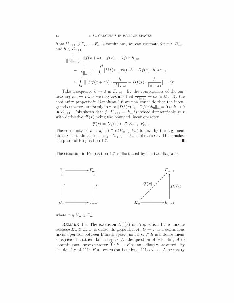
The situation in Proposition 1.7 is illustrated by the two diagrams
Um
Fm
Um−1
Fm−1
.
.
.
.
.
.
.
.
.
.
.
.
.
.
.
.
.
.
.
.
.
.
.
.
.
.
.
.
.
.
.
.
.
.
.
.
.
.
.
.
.
.
.
.
.
.
.
.
.
.
.
.
.
.
.
.
.
.
.
.
.
.
.
.
.
.
.
.
.
.
.
.
.
.
.
.
.
.
.
.
.
.
.
.
.
.
.
.
.
.
.
.
.
.
.
.
.
.
.
.
.
.
.
.
.
.
.
.
.
.
.
.
.
.
.
.
.
.
.
.
.
.
.
.
.
.
.
.
.
.
.
.
.
.
.
.
.
.
.
.
.
.
.
.
.
.
.
.
.
.
.
.
.
.
.
.
.
.
.
.
.
.
.
.
.
.
.
.
.
.
.
.
.
.
.
..
.
.
.
.
.
.
..
...
.
.
.
.
.
.
.
.....
f
.
.
.
.
.
.
.
.
.
.
.
.
.
.
.
.
.
.
.
.
.
.
.
.
.
.
.
.
.
.
.
.
.
.
.
.
.
.
.
.
.
.
.
.
.
.
.
.
.
.
.
.
.
.
.
.
.
.
.
.
.
.
.
.
.
.
.
.
.
.
.
.
.
.
.
.
.
.
.
.
.
.
.
.
.
.
.
.
.
.
.
.
.
.
.
.
.
.
.
.
.
.
.
.
.
.
.
.
.
.
.
.
.
.
.
.
.
.
.
.
.
.
.
.
.
.
.
.
.
.
.
.
.
.
.
.
.
.
.
.
.
.
.
.
.
.
.
.
.
.
.
.
.
.
.
.
.
.
.
.
.
.
.
.
.
.
.
.
.
.
.
.
.
.
.
..
.
.
.
.
.
.
..
...
.
.
.
.
.
.
.
.....
f
.............................................................................................................................................................................
............
.............................................................................................................................................................................
............
Em Em−1
Fm−1
.
.
.
.
.
.
.
.
.
.
.
.
.
.
.
.
.
.
.
.
.
.
.
.
.
.
.
.
.
.
.
.
.
.
.
.
.
.
.
.
.
.
.
.
.
.
.
.
.
.
.
.
.
.
.
.
.
.
.
.
.
.
.
.
.
.
.
.
.
.
.
.
.
.
.
.
.
.
.
.
.
.
.
.
.
.
.
.
.
.
.
.
.
.
.
.
.
.
.
.
.
.
.
.
.
.
.
.
.
.
.
.
.
.
.
.
.
.
.
.
.
.
.
.
.
.
.
.
.
.
.
.
.
.
.
.
.
.
.
.
.
.
.
.
.
.
.
.
.
.
.
.
.
.
.
.
.
.
.
.
.
.
.
.
.
.
.
.
.
.
.
.
.
.
.
..
.
.
.
.
.
.
.....
.
.
.
.
.
.
.
..
...
Df(x)
..
....................................................................................................................................................................................................................................................................................
.
...........
df(x)
.............................................................................................................................................................................
............
where x ∈ Um ⊂ Em.
Remark 1.8. The extension Df(x) in Proposition 1.7 is uniquebecause Em ⊂ Em−1 is dense. In general, if A : G → F is a continuouslinear operator between Banach spaces and if G ⊂ E is a dense linearsubspace of another Banach space E, the question of extending A toa continuous linear operator A : E → F is immediately answered. Bythe density of G in E an extension is unique, if it exists. A necessary

1.2. SC-SMOOTH MAPS 19
and sufficient condition for the existence of a continuous extension isthe existence of a positive constant C such that
‖Ah‖F ≤ C · ‖h‖E for all h ∈ G.
It is important to note that the second condition in (1.7) says that themap Um → Lco(Em−1, Fm−1) is continuous where Lco is the space ofcontinuous linear operators equipped with the compact open topology(rather than the usual operator topology).
If the sc-continuous map f : U ⊂ E → F is of class sc1, then itstangent map
Tf : TU → TF
is an sc-continuous map. If now Tf is of class sc1, then f : U → F iscalled of class sc2 . In this case the tangent map of Tf ,
T (Tf) : T (TU) → T (TF )
is sc-continuous. We shall use the notation T 2f = T (Tf) and T 2U =T (TU) and T 2F = T (TF ). Then T 2U = T (TU) = T (U1 ⊕ E) =(U2 ⊕ E1) ⊕ (E1 ⊕ E) has the sc-smooth structure
(T 2U)m = Um+2 ⊕ Em+1 ⊕ Em+1 ⊕ Em, m ≥ 0.
Proceeding this way inductively, the map f : U → F is called ofclass sck if the sc-continuous map T k−1f : T k−1U → T k−1F is of classsc1. Its tangent map T (T k−1f) is then denoted by T kf . It is a sc-continuous map T kU → T kF . A map which is of class sck for every kis called sc-smooth or of class sc∞ . To illustrate these concepts weshall prove the following consequences of the definitions.
Proposition 1.9. If f : U ⊂ E → F is of class sck, then
f : Um+k → Fm
is of class Ck for every m ≥ 0.
Proof. For k = 1 the proposition follows from our alternativedefinition (Proposition 1.7). In this case the tangent map Tf : TU →TF is of the form
Tf(x1, x2) = (f(x1), Df(x1)[x2]).
In particular, if (x1, x2) ∈ Um+1 ⊕ Em+1 ⊂ Em+1 ⊕ Em and df(x1) :Em+1 → Fm is the derivative of f at x1, then Df(x1)[x2] = df(x1)[x2].The general case follows from the following claim which we prove byinduction.

20 1. SC-CALCULUS IN BANACH SPACES
Let f : U → F be of class sck. Then f : Um+k → Fm is of classCk for all m ≥ 0. In addition, if m ≥ 0 and π is the projection of(T kF )m onto the last factor Fm, then, at every point x = (x1, . . . x2k) ∈Em+k ⊕ Em+k ⊕ · · · ⊕ Em+k ⊂ (T kU)m, the composition π ◦ T kf(x) isa linear combination of terms of the form
(1.4) djf(x1)[xi1 , . . . , xij ],
where 1 ≤ j ≤ k.
We already know that the claim is true when k = 1. Assumingthat our claim holds for k ≥ 1 we show that it is also true for a mapf : U → F of class sck+1. Given such a map f , then its tangent mapT kf : T kU → T kF is of class sc1. Thus, in view of Proposition 1.7,the map T kf : (T kU)m+1 → (T kF )m is of class C1 for every m ≥ 0.In particular, it is also of class C1 when considered as a map fromEm+k+1⊕· · ·⊕Em+k+1 ⊂ (T kU)m+1 into (T kF )m. Taking the projectionπ from (T kF )m onto the last factor Fm the composition π ◦ T kf :Em+k+1 ⊕Em+k+1 ⊕ · · · ⊕Em+k+1 → Fm is continuously differentiable.By our inductive assumption, at points x = (x1, . . . , x2k) ∈ Em+k ⊕· · · ⊕ Em+k, the map π ◦ T kf(x) is a linear combinations of maps ofthe form (1.4). Because f is Ck, every term djf(x1)[xi1 , . . . , xij ] withj ≤ k − 1 defines a C1-map whose derivative is equal to
(1.5) dj+1f(x1)[x1, xi1 , . . . , xij ] +∑
1≤l≤j
djf(x1)[xi1 , . . . , xil , . . . xij ]
where (x1, xi1 , . . . , xij ) ∈ Em+k+1 ⊕ · · · ⊕ Em+k+1.
Hence dkf(x1)[xi1 , . . . , xij ] also defines a C1 map from Em+k+1 ⊕ · · · ⊕Em+k+1 into Fm and this implies that f is of class Ck+1. Denoting bydk+1f(x1) the derivative of f of order k + 1 we see that the derivatived(π ◦ T kf)(x) of π ◦ T kf at x ∈ Em+k+1 ⊕ · · · ⊕ Em+k+1 is a linearcombination of terms (1.5) and of the term
(1.6) dk+1f(x1)[x1, xi1, . . . , xik ] +∑
1≤l≤k
djf(x1)[xi1 , . . . , xil, . . . xik ].
Hence taking a point (x, x) = (x1, . . . , x2k , x1, . . . , x2k) ∈ Em+k+1 ⊕· · · ⊕ Em+k+1 ⊂ (T k+1U)m and evaluating the composition π ◦ T k+1fat (x, x) we see that π ◦T k+1f(x, x) is a linear combination of terms ofthe form (1.4). This finishes the induction and hence the proof of theproposition. �
The following criterion for sc-smoothness will be handy later on.

1.2. SC-SMOOTH MAPS 21
Proposition 1.10. Let E be a Banach space with a sc-smoothstructure and let U ⊂ E be an open subset. Assume that f : U → R issc-continuous and that the induced maps
fm := f |Um: Um → R, m ≥ 0,
are of class Cm+1. Then f is of class sc∞.
We observe that the deeper we go down the nested sequence ofspaces the higher are the differentiability properties of the sc-smoothfunctions. The space R is, as usual, equipped with the constant sc-structure.
Proof. The proposition follows from the following statement whichwe shall prove by induction.
(k) The map f : U → R is of class sck and the iterated tangentmap T kf : T kU → T kR has the following property for every m ≥ 0.Let π : T kR → R be the projection on any factor R of T kR and letx = (x1, . . . , x2k) ∈ (T kU)m. Then the composition π ◦ (T kf)(x) is alinear combination of terms
(1.7) djf(x1)[xk1, ..., xkj],
where 0 ≤ j ≤ k and x1 ∈ Um+k and xki∈ Emi
with mi ≥ m + (j − 1).
We start with k = 1. Take x1 ∈ U1 and define the linear mapDf(x1) : E0 → R by
Df(x1)x2 = df(x1)x2
where df(x1) : E0 → R is the derivative of the map f : U0 → R. Clearly,Df(x1) ∈ L(E0, R). Since f : U1 → R is of class C2, its derivativedf(x1) : E1 → R is equal to Df(x1)|E1. Hence part (1) of Definition1.6 holds. The continuity of the map U1 ⊕E0 → R given by (x1, x2) �→Df(x1)x2 follows from the continuity of x1 �→ Df(x1) = df(x1) ∈L(E0, R). This also implies the continuity of the map Um+1 ⊕Em → Rgiven by (x1, x2) �→ Df(x1)x2 since the convergence in Um+1 ⊕ Em
implies the convergence in U1 ⊕ E0. The tangent map Tf : TU → TRhas the form
Tf(x1, x2) = (f(x1), Df(x1)x2) = (f(x1), df(x1)x2)
for (x1, x2) ∈ Um+1 ⊕ Em, m ≥ 0. We have verified the assertion (k)for k = 1.
Next assume that the statement (k) holds for k ≥ 1. Let 1 ≤ j ≤ k.Setting m = 0 at first we assume m1, . . . , mj ≥ j − 1. Abbreviate

22 1. SC-CALCULUS IN BANACH SPACES
U ′ = Uk ⊕Em1 ⊕ · · · ⊕Emjand E ′ = Ek ⊕Em1 ⊕ · · · ⊕Emj
. It sufficesto show that the map Φ : U ′ → R defined by
(1.8) Φ(x) := Φ(x1, xk1 , · · · , xkj) = djf(x1)[xk1 , · · · , xkj
]
is of class sc1. Take x = (x1, xk1, . . . , xkj) ∈ U ′
1 = Uk+1 ⊕Em1+1 ⊕ · · ·⊕Emj+1 and define the linear map
DΦ(x) : E ′0 = Ek ⊕ Em1 ⊕ · · · ⊕ Emj
→ R
by setting
DΦ(x)(y) = dj+1f(x1)[y1, xk1 , · · · , xkj]
+∑
1≤i≤j
djf(x1)[xk1 , · · · , yki, · · · , xkj
].(1.9)
Since f : Uj → R is of class Cj+1 and x1 ∈ Uk+1 ⊂ Uj and y1 ⊂ Ek ⊂ Ej
and xki⊂ Emi+1 ⊂ Ej , it follows that the map
Ek → R, y1 �→ dj+1f(x1)[y1, xk1 , · · · , xkj]
is a continuous linear operator in y1. Also the maps
Emi�→ R, yki
�→ djf(x1)[xk1 , · · · , yki, · · · , xkj
]
are continuous linear maps. Consequently, DΦ(x) : E ′0 → R is a contin-
uous linear operator. Moreover, the map Φ : U ′1 → R is of class C1 and
its derivative dΦ(x) at the point x ∈ U ′1 coincides with DΦ(x)|E ′
1. Thisshows that condition (1) of Definition 1.6 is satisfied. Note also that if(xn, yn) ∈ U ′
1 ⊕ E ′0 converges in U ′
1 ⊕ E ′0, then DΦ(xn)yn converges in
R and since the convergence in U ′m+1 ⊕ Em implies the convergence in
U ′1 ⊕ E ′
0 we conclude the continuity of the map (x, y) �→ DΦ(x)y fromU ′
m+1 ⊕ E ′m into R. The tangent map TΦ : TU ′ → TR has the form
TΦ(x, y) = (Φ(x), DΦ(x)(y))
where Φ(x) is given by (1.8) and DΦ(x)(y) by formula (1.9) for (x, y) ∈TU ′ = (U ′)1⊕E ′ = (Uk+1⊕Em1+1⊕· · ·⊕Emj+1)⊕(Ek⊕Em1⊕· · ·⊕Emj
).The tangent map Tf is of class sc0 by the above remark. Inspecting theterms of Φ(x) and DΦ(x)(y) we see that the components of TΦ(x, y) areof the form (1.7) with indices satisfying the conditions in (k) however,with k replaced by k + 1. Hence the statement (k+1) holds true andthe proof of Proposition 1.10 is complete. �
The next and more general criterion for sc-smoothness is provedthe same way as Proposition 1.10.

1.2. SC-SMOOTH MAPS 23
Proposition 1.11. Let E and F be sc-Banach spaces and let U ⊂E be open. Assume that the map f : U → F is sc0 and that the inducedmap f : Um+k → Fm is Ck+1 for every m, k ≥ 0. Then f : U → E issc-smooth.
The example coming up has many of the features of situations weare confronted with in the SFT, but is a little bit easier. It illustratesthe sharp contrast between the new concept of sc-smoothness and theclassical smoothness concept.
Example 1.12. The R-action of translation
Φ : R ⊕ E → E, (t, u) �→ t ∗ u
introduced in (1.1) is an sc-smooth map. The spaces are equipped withthe previously defined sc-structures. The tangent map
TΦ : R ⊕ E1 ⊕ R ⊕ E → E1 ⊕ E
is given by
(TΦ)(t, u)[δt, δu] =
(t ∗ u, δt
(t ∗
du
dt
)+ t ∗ (δu)
).
This more difficult result is proved in Theorem 1.38 below. Here theincreasing weights play a decisive role.
We point out that Φ is not differentiable with respect to t in theclassical sense due to the loss of derivatives.
Taking the derivative of a function f or g, the target levels dropby 1 according to Proposition 1.7. Therefore, one could expect for thecomposition g ◦ f of the two maps, that the target level should dropby 2 in order to obtain a C1-map. As it turns out, however, this is notthe case.
Theorem 1.13 (Chain Rule). Assume that E, F and G are sc-smooth Banach spaces and U ⊂ E and V ⊂ F are open sets. Assumethat f : U → F and g : V → G are of class sc1 and f(U) ⊂ V . Thenthe composition g ◦ f : U → G is of class sc1 and the tangent mapssatisfy
T (g ◦ f) = (Tg) ◦ (Tf).
Proof. We shall verifiy properties (1) and (2) in Definition 1.6 forg ◦ f . From Proposition 1.7 we conclude that the functions g : V1 → Gand f : U1 → F are of class C1. Moreover, Dg(f(x))◦Df(x) ∈ L(E, G)
24 1. SC-CALCULUS IN BANACH SPACES
if x ∈ U1. Fix x ∈ U1 and choose h ∈ E1 sufficiently small so thatf(x + h) ∈ V 1. Then, using the postulated properties of f and g,
g(f(x + h)) − g(f(x)) − Dg(f(x)) ◦ Df(x)h
=
∫ 1
0
Dg(tf(x + h) + (1 − t)f(x)) [f(x + h) − f(x) − Df(x)h]dt
+
∫ 1
0
([Dg(tf(x + h) + (1 − t)f(x)) − Dg(f(x))] ◦ Df(x)h
)dt.
Consider the first term(1.10)
1
‖h‖1
∫ 1
0
Dg(tf(x + h) + (1 − t)f(x))[f(x + h) − f(x) − Df(x)h]dt
=
∫ 1
0
Dg(tf(x + h) + (1 − t)f(x)) ·1
‖h‖1
[f(x + h) − f(x) − Df(x)h]dt.
If h ∈ E1, the maps [0, 1] → Fm defined by t → tf(x+h)+(1−t)f(x)are continuous and converge in C0([0, 1], F1) to the constant map t →f(x) as ‖h‖1 → 0. Moreover, since f is of class sc1,
a(h) :=1
‖h‖1
[f(x + h) − f(x) − Df(x)h
]converges to 0 in F0 as ‖h‖1 → 0. Therefore, by the continuity as-sumption (2) in Definition 1.6, the map
(t, h) → Dg(tf(x + h) + (1 − t)f(x))[a(h)]
as a map from [0, 1]×E1 into G0 converges to 0 as h → 0, uniformly int. Consequently, the expression in (1.10) converges to 0 in G0 as h → 0in E1. Next consider the second integral
(1.11)
∫ 1
0
[Dg(tf(x + h) + (1− t)f(x))−Dg(f(x))
]◦Df(x)
h
‖h‖1dt.
The set of all h‖h‖1
∈ E1 has a compact closure in E0, in view of Defi-
nition 1.1, so that the closure of the set of all
Df(x)h
‖h‖1
is compact in F0 because Df(x) ∈ L(E0, F0) is a continuous map byDefinition 1.6. Consequently, again by property (2) of Definition 1.1,every sequence hn converging to 0 in E1 possesses a subsequence havingthe property that the integrand of the integral in (1.11) converges to 0

1.2. SC-SMOOTH MAPS 25
in G0 uniformly in t. Hence the integral (1.11) also converges to 0 inG0 as h → 0 in E1. We have proved that
1
‖h‖1
‖g(f(x + h)) − g(f(x)) − Dg(f(x)) ◦ Df(x)h‖0 → 0
as h → 0 in E1. Consequently, condition (1) of Definition 1.6 is satisfiedfor the composition g ◦ f with the operator
D(g ◦ f)(x) = Dg(f(x)) ◦ Df(x) ∈ L(E0, G0),
where x ∈ U1. We conclude that the tangent map T (g◦f) : TU → TG,
(x, h) �→ ( g ◦ f(x), D(g ◦ f)(x)h )
is sc-continuous and, moreover, T (g ◦ f) = Tg ◦ Tf . The proof ofTheorem 1.13 is complete. �
The reader should realize that in the previous proof all conditions on sc1
maps were used, i.e. it just works. From Theorem 1.13 one concludesby induction that the composition of two sc∞-maps is also of class sc∞
and, for every k ≥ 1,
T k(g ◦ f) = (T kg) ◦ (T kf).
Remark 1.14. There are other possibilities for defining new smooth-ness concepts. For example, we can drop the requirement of compact-ness of the embedding operator En → Em for n > m. Then it isnecessary to change the definition of smoothness in order to get thechain rule. One needs to replace the second condition in the defini-tion of being sc1 by the requirement that Df(x) induces a continuouslinear operator Df(x) : Em−1 → Fm−1 for x ∈ Um and that the mapUm → L(Em−1, Fm−1) for m ≥ 1 is continuous. For this theory the sc-smooth structure on E given by Em = E recovers the usual Ck-theory.However, this modified theory seems not to be applicable to SFT. Inparticular, the R-action of translation in Example 1.12 would alreadyfail to be smooth using this alternative concept of smoothness.
A sc-diffeomorphism f : U → V , where U and V are open subsetsof sc-spaces E and F with the induced sc-structure*, is by definitiona homeomorphism U → V so that f and f−1 are sc-smooth. Letus note that in view of Theorem 1.13 we can define the pseudogroupof local sc-diffeomorphisms. As a corollary we obtain the category of
*In the following we will sometimes say that a Banach space has a sc-structurerather than a sc-smooth structure.

26 1. SC-CALCULUS IN BANACH SPACES
sc-manifolds consisting of second countable paracompact topologicalspaces equipped with a maximal atlas of sc-smoothly compatible charts.We will develop this concept later on where we will illustrate it withsome examples.
1.3. sc-Operators
We need several definitions.
Definition 1.15. Consider E equipped with a sc-smooth structure.
• An sc-smooth subspace F of E consists of a closed linearsubspace F ⊆ E, so that Fm = F ∩ Em defines a sc-smoothstructure for F in the sense of Definition 1.1.
• An sc-smooth subspace F of E splits if there exists an-other sc-smooth subspace G so that on every level we have thetopological direct sum
Em = Fm ⊕ Gm
We shall use the notation
E = F ⊕sc G.
Definition 1.16. Let E and F be sc-smooth Banach spaces.
• An sc-operator T : E → F is a bounded linear operatorinducing bounded linear operators on all levels
T : Em → Fm.
• An sc-isomorphism is a surjective sc-operator T : E → Fsuch that T is invertible and T−1 : E → F is also an sc-operator.
It is useful to point out that a finite-dimensional subspace K of Ewhich splits the sc-smooth space E necessarily belongs to E∞.
Proposition 1.17. Let E be a sc-smooth Banach space and K afinite-dimensional subspace of E∞. Then K splits the sc-space E.
Proof. Take a basis e1, ..., en for K and fix the associated dualbasis. By Hahn Banach this dual basis can be extended to continuouslinear functionals λ1, ..., λn on E. Now P (h) =
∑ni=1 λi(h)ei defines a
continuous projection on E with image in K ⊂ E∞. Hence P inducescontinuous maps Em → Em. Therefore P is a sc-projection. DefineYm = (Id − P )(Em). Setting Y = Y0 we have E = K ⊕ Y . We claimthat Ym = Em ∩ Y0. By construction, Ym ⊂ Em ∩ Y0. An element

1.3. SC-OPERATORS 27
x ∈ Em ∩ Y0 has the form x = e − P (e) with x ∈ Em and e ∈ E0.Since P (e) ∈ E∞ we see that e ∈ Em, implying our claim. Finally,Y∞ = ∩m≥0Ym is dense in Ym for every m ≥ 0. Indeed, if x ∈ Ym, wecan choose xk ∈ E∞ satisfying xk → x in Em. Then (Id − P )xk ∈ Y∞
and (Id − P )xk → (Id − P )x = x in Ym. �
We can introduce the notion of a linear Fredholm operator in thesc-setting.
Definition 1.18. Let E and F be sc-smooth Banach spaces. Asc-operator T : E → F is called Fredholm provided there exist sc-splittings E = K ⊕sc X and F = Y ⊕sc C with the following properties.
• K = kernel (T ) is finite-dimensional.
• C is finite-dimensional.
• Y = T (X) and T : X → Y defines a linear sc-isomorphism.
The above definition implies T (Xm) = Ym, that the kernel of T :Em → Fm is K and that C spans its cokernel, so that
Em = ker T ⊕ Xm and Fm = T (Em) ⊕ C
for all m ∈ N. The following observation, called the regularizing prop-erty, should look familiar.
Proposition 1.19. Assume T : E → F is sc-Fredholm and
Te = f
for some e ∈ E0 and f ∈ Fm. Then e ∈ Em.
Proof. Since Fm = T (Em) ⊕ C, the element f ∈ Fm has therepresentation
f = T (x) + c
for some x ∈ Xm and c ∈ C. Similarly, e has the representation
e = k + x0,
with k ∈ K = ker T and x0 ∈ X0 because E0 = K ⊕ X0. FromT (e) = f = T (x) + c and T (x) = T (x0) one concludes T (x0 − x) = c.Hence c = 0 because T (E0) ∩ C = {0}. Consequently, x0 − x ∈ K.Since e − x = k + (x0 − x) ∈ K, x ∈ Em, and K ⊂ Em one concludese ∈ Em as claimed. �

28 1. SC-CALCULUS IN BANACH SPACES
We end this subsection with an important definition and stabilityresult for Fredholm maps.
Definition 1.20. Let E and F be sc-Banach spaces. An sc-operatorR : E → F is said to be an sc+
− operator if R(Em) ⊂ Fm+1 and ifR induces a sc0-operator E → F1.
Let us note that due to the (level-wise) compact embedding F1 → Fa sc+-operator induces on every level a compact operator. This followsimmediately from the factorization
R : E → F 1 → F.
The stability result is the following statement.
Proposition 1.21. Let E and F be sc-Banach spaces. If T : E →F is a sc-Fredholm operator and R : E → F a sc+-operator, then T +Ris also a sc-Fredholm operator.
Proof. Since R : Em → Fm is compact for every level we see thatT + R : Em → Fm is Fredholm for every m. Let Km be the kernelof T + R : Em → Fm. We claim that Km = Km+1 for every m ≥ 0.Indeed, Km+1 ⊂ Km. If x ∈ Km, then Tx = −Rx ∈ Fm+1. ApplyingProposition 1.19, x ∈ Em+1 so that x ∈ Km+1. Hence the kernel Km
is independent of m. Set K = K0. By Proposition 1.17, K splits thesc-space E since it is a finite dimensional subset of E∞. Hence we havethe sc-splitting E = K ⊕ X for a suitable sc-subspace X. Next defineYm = (T + R)(Em). This defines a sc-structure on Y = Y0. Let usshow that F induces a sc-structure on Y and that this is the one givenby Ym. For this it suffices to show that
(1.12) Y ∩ Fm = Ym.
Clearly,
Ym = (T +R)(Em) ⊂ Fm∩(T +R)(Em) ⊂ Fm∩(T +R)(E0) = Y ∩Fm.
Next assume that y ∈ Y ∩Fm. Then there exists x ∈ E0 with Tx+Rx =y. Since R is a sc+-section it follows that y − Rx ∈ F1 implying thatx ∈ E1. Inductively we find that x ∈ Em implying that y ∈ Ym and(1.12) is proved. Observe that we also have
F∞ ∩ Y = (⋂
m∈N
Fm) ∩ Y =⋂
m∈N
(Fm ∩ Y ) =⋂
m∈N
Ym = Y∞
In view of Lemma 1.22 below, there exists a finite dimensional sub-space C ⊂ F∞ satisfying F0 = C ⊕ Y . From this it follows that

1.3. SC-OPERATORS 29
Fm = C ⊕ Ym. Indeed, since C ∩ Ym ⊂ C ∩ Y , we have C ∩ Ym = {0}.If f ∈ Fm, then f = c + y for some c ∈ C and y ∈ Y since Fm ⊂ Yand F0 = C ⊕Y . Hence y = f − c ∈ Fm and using Proposition 1.19 weconclude y ∈ Fm. This implies, in view of (1.12), that Fm = C ⊕ Ym.We also have F∞ = C ⊕ (F∞ ∩ Y ) = C ⊕ Y∞. It remains to showthat Y∞ is dense in Ym for every m ≥ 0. Since Fm = C ⊕ Ym with Cfinite-dimensional and Ym closed, the norm ‖c + y‖ = ‖c‖m + ‖y‖m isequivalent to the norm ‖c+y‖m. Take y ∈ Ym. Then since F∞ is densein Fm we find sequences cn ∈ C and yn ∈ Y∞ such that cn + yn → yin Fm. From the above remark about equivalent norms we concludethat the sequence cn is bounded and we may assume cn → c. Hencethe sequence yn converges to some y′ ∈ Ym because Y∞ ⊂ Ym and Ym
is closed. Thus, c + y′ = y so that c = 0 and yn → y in Fm, provingour claim. Consequently, we have the sc-splitting
F = Y ⊕sc C
and the proof of the proposition is complete. �
Lemma 1.22. Assume F is a Banach space and F = D⊕Y with Dof finite-dimension and Y a closed subspace of F . Assume, in addition,that F∞ is a dense subspace of F . Then there exists a finite dimensionalsubspace C ⊂ F∞ such that F = C ⊕ Y .
Proof. Denoting by d1, . . . , dn a basis of D we define the finite
dimensional subspaces Ni of F by setting Ni = span{d1, . . . , di, . . . , dn}
where di means that the vector di is omitted. The space Ni⊕Y is closedand since di �∈ Ni ⊕ Y we have εi := dist(di, Ni ⊕ Y ) > 0. Choose0 < ε < mini εi. In view of the fact that F∞ is dense in F we find,for every 1 ≤ i ≤ n, an element ci ∈ F∞ satisfying ‖di − ci‖ < ε/(2n).The vectors c1, . . . , cn are linearly independent. Indeed, arguing bycontradiction we assume
∑i αici = 0 with
∑i|αi| > 0. Without loss
of generality we may also assume |α1| ≥ |α2|, . . . , |αn|. Hence c1 =∑i≥2(−αi/α1)ci =
∑i≥2 βici with |βi| ≤ 1. Then one estimates
ε
2n> ‖d1 − c1‖ = ‖c1 −
∑i≥2
βici‖ = ‖(d1 −∑i≥2
βidi) −∑i≥2
βi(ci − di)‖
≥ ‖d1 −∑i≥2
βidi‖ −∑i≥2
|βi|‖ci − di‖ ≥ ε −n − 1
2nε >
ε
2n.
This contradiction shows that the vectors ci are linearly independent.Abbreviating C := span{c1, . . . , cn} we will show that C ∩ Y = {0}.Once again arguing by contradiction we assume that
∑i αici ∈ Y for
30 1. SC-CALCULUS IN BANACH SPACES
some constants αi satisfying∑
i|αi| > 0. We may assume |a1| ≥|a2|, . . . , |αn| so that c1 +
∑i≥2 βici ∈ Y where βi = αi/α1. Note that
(−∑
i≥2 βidi) + (c1 +∑
i≥2 βici) ∈ Ni ⊕ Y . Since dist(d1, N1 ⊕ Y ) =εi > ε, we reach a contradiction as the following estimates show,
ε < ε1 ≤ ‖d1 −[−
∑i≥2
βidi + (c1 +∑i≥2
βici)]‖
= ‖(d1 − dc1) +∑i≥2
βi(di − ci)‖ ≤∑i≥1
‖di − ci‖ ≤ n ·ε
2n=
ε
2.
Finally, we prove F = C ⊕Y . Since C and D have the same dimensionthere is a linear isomorphism ψ : C → D. Define Ψ : C⊕Y → D⊕Y byΨ(c+y) = ψ(c)+y. Then Ψ is injective and since Ψ(ψ−1(d)+y) = d+yit is also surjective. Hence C ⊕ Y = D⊕ Y = F as claimed. The proofof the lemma is complete. �
1.4. sc-Manifolds
In this section we are going to introduce the spaces needed to for-mulate the general Fredholm theory.
1.4.1. Topological Considerations. We start by recalling somedefinitions.
Definition 1.23. Let X be a topological space.
• The space X is said to be second countable if it has a countablebasis for its topology.
• The space X is said to be completely regular if for every pointx ∈ X and every neighborhood U(x) of x there exists a con-tinuous map f : X → [0, 1] satisfying f(x) = 0 and f(y) = 1for all y ∈ X \ U(x).
• A space X is said to be normal provided it is Hausdorff anddisjoint closed subsets admit disjoint open neighborhoods.
• A space X is said to be paracompact if it is Hausdorff and forevery open covering of X there exists a finer open coveringwhich is locally finite.
The crucial result concerning paracompact spaces is the existenceof partitions of unity, see for example Dugundji [6].
Proposition 1.24. If X is a paracompact space and U an opencovering of X, then there exists a sub-ordinate partition of unity.
The following is a useful classical result by Urysohn.

1.4. SC-MANIFOLDS 31
Proposition 1.25. For a second countable topological space thenotions of being normal or completely regular or metrizable are equiv-alent.
An obvious consequence is the following corollary.
Corollary 1.26. A second countable Hausdorff space X which islocally homeomorphic to open subsets of Banach spaces is metrizableand hence, in particular, paracompact.
Proof. The space X is completely regular since it is locally homeo-morphic to open subsets of Banach spaces. Therefore, as a consequenceof Proposition 1.25, the space X is metrizable and hence paracom-pact. �
1.4.2. sc-Manifolds. Using the results so far we can define sc-manifolds. This concept will not yet be sufficient to describe the spacesarising in SFT. However, certain components of the ambient spaceshave subspaces which will inherit the structure of an sc-manifold.
Definition 1.27. Let X be a second countable Hausdorff space. Ansc-chart for X consists of a triple (U, ϕ, E), where U is an open subsetof X, E a Banach space with a sc-smooth structure and ϕ : U → E isa homeomorphism onto an open subset V of E. Two such charts aresc-smoothly compatible provided the transition maps are sc-smooth. Ansc-smooth atlas consists of a family of charts whose domains coverX so that any two charts are sc-smoothly compatible. A maximal sc-smooth atlas is called a sc-smooth structure on X . The space Xequipped with a maximal sc-smooth atlas is called an sc-manifold .
Let us observe that a second countable Hausdorff space which ad-mits an sc-smooth atlas has to be metrizable and paracompact since itis locally homeomorphic to open subsets of Banach spaces.
As a side remark we also note that the above construction addressescertain issues arising in the analysis underlying Gromov-Witten theory.For example, if we have a holomorphic curve with an unstable domaincomponent we have to divide out by a non-discrete group. These issueswill arise later when we construct the ambient spaces for SFT.
Assume that X has a sc-smooth structure. Then it possesses thefiltration given by Xm for all m ≥ 0, from which every Xm inherits ansc-smooth structure. We shall define the tangent bundle TX → X1 in
32 1. SC-CALCULUS IN BANACH SPACES
a natural way so that the tangent projection is sc-smooth*. In order todo so we use an appropriate modification of the definition found, forexample, in Lang’s book [16]. Namely consider tuples (U, ϕ, E, x, h)where (U, ϕ, E) is a sc-smooth chart, x ∈ U1 and h ∈ E. Call twosuch tuples equivalent provided x = x′ and D(ϕ′ ◦ ϕ−1)(ϕ(x))h = h′.An equivalence class [U, ϕ, E, x, h] is called a tangent vector. Denotethe whole collection of tangent vectors by TX. We have a canonicalprojection p : TX → X1. We define for an open subset U ⊂ X the setTU by TU = p−1(U ∩ X1) . For a chart (U, ϕ, E) we define the map
Tϕ : TU → E1 ⊕ E
by
Tϕ([U, ϕ, E, x, h]) = (x, h).
One easily checks that the collection of all these maps defines a smoothatlas for TX and that the projection p is sc-smooth.
1.5. A Space of Curves
This section is the first installment of several sections in which weillustrate the abstract concepts in the classical Morse theory. Recallthat for a Morse function f : M → R on the compact Riemannianmanifold M one studies the gradient flow on M defined by the equation
x(s) = ∇f(x(s)), s ∈ R
x(0) = x ∈ M.
Every solution x(s) converges as s → ∞ and s → ∞ to critical pointsof the function f . The aim is to investigate the structure of the set ofall these orbits connecting critical points and, moreover, the compact-ifications of these solution spaces consisting of broken trajectories.
For simplicity we first consider a set of curves in Rn connecting thepoint a ∈ Rn at −∞ with the point b ∈ Rn at ∞, where a �= b. Wefirst choose a smooth reference curve ϕ : R → Rn connecting the twopoints and satisfying
ϕ(s) = a for s ≤ −1 and ϕ(s) = b for s ≥ 1.
*The definition of sc-smooth maps between sc-manifolds is the obvious modifi-cation from standard manifold theory.

1.5. A SPACE OF CURVES 33
Then we equip the Sobolev space E = H2(R, Rn) with the sc-smoothstructure Em = Hm+2,δm , where δ0 = 0 < δ1 < · · · is a strictly increas-ing sequence of weights. Now we introduce the space
X = {u = ϕ + h| h ∈ E}
of parametrized curves u : R → Rn connecting the point a at −∞ withthe point b at +∞ and having Sobolev regularity equal to 2.
a
b
u
Figure 1.1
The topology of X is induced by the complete metric d on X,
d(u, v) = ‖u − v‖0
where the norm on the right hand side is the Sobolev norm on E = E0.The metric is invariant under the R-action of translation,
d(t ∗ u, t ∗ v) = d(u, v)
for all t ∈ R and u, v ∈ X. In order to divide out the R-action we definean equivalence relation calling two elements in X equivalent, u ∼ v, ifthere exists a constant t ∈ R satisfying
u(s) = (t ∗ v)(s) = v(s + t) for all s ∈ R.
By [u] we shall denote the equivalence class containing u. The quotientspace
X = X/ ∼

34 1. SC-CALCULUS IN BANACH SPACES
consisting of the equivalence classes is equipped with the quotienttopology which, as we show next, is determined by a complete met-ric. We define d : X × X → [0,∞) by
d(α, β) = inf{d(u, v)| u ∈ α, v ∈ β}.
Lemma 1.28. The function d is a complete metric on X.
Proof. Clearly d is symmetric. Let [u1], [u2] and [u3] be three ele-
ments in X. Given ε > 0 we find representatives u1, u2 in X satisfying
d(u1, u2) ≤ d([u1], [u2]) + ε
and representatives u′2 of [u2] and u3 of [u3] so that
d(u′2, u3) ≤ d([u2], [u3]) + ε.
Now u′2 and u2 belong to the same orbit of the R-action. Using the
R-invariance of d we may therefore assume, replacing u3 by some otherrepresentative, that u2 = u′
2. Hence,
d(u1, u3) ≤ d([u1], [u2]) + d([u2], [u3]) + 2ε.
This implies the triangle inequality for d. Finally, we have to show thatd(α, β) = 0 implies α = β. If d(α, β) = 0 we find sequences tn, sn andrepresentatives u and v of α and β such that
d(tn ∗ u, sn ∗ v) → 0.
By the R-invariance,
d(tn ∗ u, sn ∗ v) =‖ tn ∗ u − sn ∗ v ‖0=‖ (tn − sn) ∗ u − v ‖0 .
Thus, setting τn = tn − sn,
‖τn ∗ u − v‖0 → 0.
The sequence τn is bounded. Indeed, if τn → ∞ (for some subsequence),then one concludes from the definition of ϕ, using a �= b, that ‖τn ∗u − v‖0 → ∞. Similarly, the sequence τn cannot have a subsequenceconverging to −∞. Hence, after taking a subsequence we may assumethat τn → τ0. This implies τ0 ∗ u = v implying α = β. We have provedthat d defines a metric on X implying that X is paracompact.
Next we show that the metric space (X, d) is complete. Given aCauchy-sequence αn ∈ X we can take a fast subsequence αnj
satisfyingd(αnj+1
, αnj) < 2−j. Pick a representative u1 for αn1 . Then we find a
representative u2 of αn2 satisfying
d(u2, u1) < d(αn2, αn1) + 2−1.

1.5. A SPACE OF CURVES 35
Then we can take a representative u3 of αn3 (applying the alreadypreviously used R-invariance) so that
d(u3, u2) < d(αn3, αn2) + 2−2.
Inductively we choose representatives uj+1 ∈ X satisfying
d(uj+1, uj) < d(αnj+1, αnj
) + 2−j ≤ 2−j+1.
Hence (uj) is a Cauchy sequence in X and therefore has a limit w ∈ X.By construction,
limj→∞
αnj= [w],
implying that the subsequence (αnj) and hence the whole sequence (αn)
converges, showing that the metric space (X, d) is complete. �
The projection map
p : X → X : u → [u]
satisfies
d([u], [v]) ≤ d([u], [v]).
Moreover, the map p is open. Indeed,
p−1(p(U)) =⋃t∈R
t ∗ U.
Consequently, p−1(p(U)) is open if U is open, implying, by definitionof the quotient topology of X, that p(U) is open. We leave it as anexercise to prove that d determines the quotient topology. The spaceE is separable since it can be viewed as a closed linear subspace ofa three-fold product of L2-spaces which are known to be separable.(For example, rational linear combinations of characteristic functionsof closed intervals with rational boundaries constitute a countable densesubset). For a dense sequence uj in X, the sequence αj = [uj] is densein X. Now taking metric balls with rational radii around these pointswe obtain a countable basis for the topology on X. We have provedthe following statement.
Lemma 1.29. The previously constructed space X is a completemetric space with a countable dense subset. In particular, it is a secondcountable paracompact space. Moreover, the projection map
p : X → X
is continuous and open.

36 1. SC-CALCULUS IN BANACH SPACES
Next we show that X carries the structure of a sc-manifold. Fix aclass [u] which is represented by
(1.13) u = φ + h0 for some h0 ∈ E∞.
Let Σ = Σu be an affine hyperplane in Rn such that the path u in-tersects Σ transversally for some parameter value t0. Using the R-action we may assume that t0 = 0. Recall the continuous embeddingE ↪→ C1(R, Rn) by the Sobolev embedding theorem.
a
b
Σu(0)
u = ϕ + h0 ∈ ϕ + E∞
Figure 1.2
Lemma 1.30. Consider the path u as described in (1.13). Thenthere exists a real number ε > 0 such that for every h ∈ E satisfying
‖h‖C1([−ε,ε],Rn) < ε2,
the path u + h has a unique intersection with Σ at some time t(h) ∈(−ε, ε). In addition, defining the open subset U ⊂ E by
U = {h ∈ E| ‖h‖C1([−ε,ε],Rn) < ε2},
the map h �→ t(h) from U into R is sc-smooth.

1.5. A SPACE OF CURVES 37
Proof. We represent the hyperplane Σ as Σ = {x ∈ Rn|λ(x) = c}for a linear map λ : Rn → R and a constant c ∈ R. By assumption,λ(u(0)) = c and λ(u′(0)) �= 0 since u intersects Σ transversally at timet = 0. Now introduce the function F : [−ε, ε]×C1([−ε, ε], Rn) → R by
F (t, h) = λ(u(t) + h(t)) − c.
Then F (0, 0) = 0 and the derivative dtF (0, 0) of F with respect tot at the point (0, 0) is equal to dtF (0, 0) = λ(u′(0)) �= 0. Using theimplicit function theorem one finds ε > 0 and, for every h satisfying‖h‖C1([−ε,ε],Rn) < ε2, a unique time t(h) ∈ (−ε, ε) solving the equationF (t(h), h) = 0 and satisfying t(0) = 0. In addition, the map h �→ t(h)is of class C1. This shows that u + h intersects Σ at a unique timein (−ε, ε) given by t(h). In order to prove the second statement inthe lemma we take the sc-smooth space F = H2((−ε, ε), Rn) with thenested sequence Fm = Hm+2((−ε, ε), Rn) of Sobolev spaces. Define theopen subset V ⊂ E by V = {h ∈ F | ‖h‖C1([−ε,ε],Rn) < ε2} filtrated byV m := V ∩Fm for all m ≥ 0. Since F ⊂ C1([−ε, ε], Rn) is continuouslyembedded, the function h �→ t(h) from V 0 → R is continuously dif-ferentiable. Now consider the map h �→ t(h) from V m into R and usethe fact that Fm ⊂ Cm+1([−ε, ε], Rn) is continuously embedded. Sinceu ∈ C∞([−ε, ε], Rn), the map F : [−ε, ε] × Cm+1([−ε, ε], Rn) → R isof class Cm+1. By the implicit function theorem and the Sobolev em-bedding theorem again the map h �→ t(h) from V m into R is also ofclass Cm+1. Consequently, Proposition 1.10 implies the sc-smoothnessof the map h �→ t(h) from V ⊂ F into R. Finally, defining the openset U ⊂ E by U = {h ∈ E| ‖h‖C1([−ε,ε],Rn) < ε2}, the compositionU → V → R given by h �→ t(h|[−ε,ε]) =: t(h) is also sc-smooth asclaimed in Lemma 1.30. �
Lemma 1.31. Given δ > 0 there exists a number ε1 > 0 so that thefollowing holds. If h, k ∈ E satisfy |h(s)|, |k(s)| < ε1 for all s ∈ R and
t ∗ (u + h) = u + k
for some t ∈ R, then |t| < δ.
Proof. Arguing indirectly assume that for a given δ > 0 such anumber ε1 > 0 cannot be found. Then we find sequences (hj) and (kj)in E converging uniformly to 0 and a sequence (tj) of real numbers sothat |tj| ≥ δ and
tj ∗ (u + hj) = u + kj .
If the sequence (tj) has a converging subsequence and t is its limit, thent ∗ u = u. This implies that t = 0 which contradicts |t| ≥ δ. Hence

38 1. SC-CALCULUS IN BANACH SPACES
tj → ±∞. Consider the case +∞. From
(u + hj)(tj + s) = (u + kj)(s)
we conclude as tj → ∞ that
b = u(s)
for all s. However, if s � 0 we know that u(s) is close to the pointa �= b giving a contradiction. This completes the proof. �
Finally, we are able to introduce sc-smooth charts on the metric
space X. We fix a class [u] ∈ X with the smooth representative u ∈ Xas described in (1.13) and recall that u intersects the hyperplane Σ ⊂Rn at u(0) ∈ Σ transversally.
We choose δ = ε in Lemma 1.31 where ε > 0 is the number guaran-teed by Lemma 1.30 and let ε1 > 0 be the number associated with δ inLemma 1.31. Let ΣT be the tangent plane of Σ such that Σ = u(0)+ΣT .Denote by F the codimension 1 subspace of E consisting of all h sat-isfying h(0) ∈ ΣT . Let U ⊂ F be the open neighborhood of 0 ∈ Fconsisting of all h ∈ F satisfying
‖ h ‖C1([−ε,ε]) < ε2
and|h(s)| < ε1 for all s ∈ R.
Then we define
A : U ⊂ F → X by A(h) = [u + h],
where u is the distinguished path from (1.13). Geometrically, h rep-resents a small vector field along a smooth curve u such that h(s) ∈Tu(s)R
n. We have identified the tangent space Tu(s)Rn at the point u(s)
with Rn itself and have used the exponential map of the Euclidean met-ric on Rn to present the curves near u by expu(s)(h(s)) = u(s) + h(s).All these curves connect the point a ∈ Rn at s = −∞ with the pointb ∈ Rn at s = ∞.
Lemma 1.32. The map A is a homeomorphism of U ⊂ F onto someopen subset of X.
Proof. In order to prove that A is injective we assume A(h) =A(k). Then
t ∗ (u + h) = u + k
1.5. A SPACE OF CURVES 39
for some t ∈ R. Because |h(s)|, |k(s)| < ε1 for all s we deduce fromLemma 1.31 that |t| < δ = ε. Since ‖h‖C1([−ε,ε]) < ε2 there is, byLemma 1.30, a unique point t(h) ∈ (−ε, ε) so that (u + h)(t(h)) ∈ Σ.Since h ∈ F and hence (u + h)(0) ∈ Σ we must have t(h) = 0 andconsequently h = k. This shows that the map A is injective. ClearlyA is continuous.
Let us finally show that A is open. Assume [u0] = A(h0) for someh0 ∈ U . We find t0 ∈ R such that
t0 ∗ u0 = u + h0.
Taking the appropriate representative for u0 we may assume that t0 = 0so that u0(0) ∈ Σ. Since h0 ∈ U we have
‖h0‖C1([−ε,ε]) < ε2
|h0(s)| < ε1 for all s ∈ R.
By the definition of the topology on X, an open neighborhood of [u0] isgenerated by taking the equivalence classes of the elements of an openneighborhood of the representative u0. Thus we take a sufficiently smallopen neighborhood V1 ⊂ X of u0 so that for v ∈ V1 we still have
‖v − u‖C1([−ε,ε]) < ε2
and
|v(s) − u(s)| < ε1 for all s ∈ R.
Since v = u+(v−u) there exists by Lemma 1.30 a unique t(v) ∈ (−ε, ε)such that v(t(v)) ∈ Σ. Now define
P (v) := t(v) ∗ v − u.
If v = u0, so that v = u + h0 we conclude from h0(0) ∈ ΣT that(u + h0)(0) ∈ Σ. Hence t(v) = t(u0) = 0 and consequently P (u0) =u+h0−u0 = h0 ∈ F . It follows from the definition that P (v) ∈ F . Since
by Lemma 1.30 the map v �→ t(v) from V1 ⊂ X into R is continuousand since the R-action by Theorem 1.38 is sc-smooth, the composition
v �→ (t(v), v) �→ t(v) ∗ v − u = P (v)
from V1 into F is continuous. Therefore, if v is close enough to u0 then
P (v) lies in U . Since V1 is open in X and since [v] = [u + (v − u)] =[u + P (v)] we have proved that the map A is open, and the proof ofLemma 1.32 is complete. �
From Lemma 1.32 we conclude that the map
Φ = A−1

40 1. SC-CALCULUS IN BANACH SPACES
defines an sc-chart on X whose domain is the open set A(U) ⊂ X. Wenext show that the transition maps are sc-smooth.
Lemma 1.33. Assume that Φ : O → U and Φ′ : O′ → V are sc-charts with O ∩ O′ �= ∅ as described above. Then the transition map
Φ′ ◦ Φ−1 : Φ(O ∩ O′) → Φ′(O ∩ O′)
is sc-smooth.
Proof. In view of the definition of an sc-chart we have Φ = A−1
and Φ′ = A′−1 where
A : U → O
A(h) = [u + h]
and where
A′ : V → O′
A′(k) = [v + k]
with U and V as described above, and with the paths u and v on the∞-level. Assume
[u + h0] = [v + k0]
for some h0 in U and k0 in V . Then
t0 ∗ (u + h0) = v + k0
for some real number t0. Evaluating at s = 0 we conclude (u+h0)(t0) =v(0)+k0(0) ∈ Σv, where Σv is the hypersurface used in the constructionof the “v-chart”. Using the implicit function theorem as in Lemma1.30 we find an sc-smooth map h �→ t(h) defined for h close to h0 in Eso that the path (u + h) intersects Σv transversally at the parametervalue t(h), and, in addition, satisfies t(h0) = t0. Now the transitionmap Φ′ ◦ Φ−1 = A′−1 ◦ A near h0 is the map
h → t0(h) ∗ (u + h) − v.
Since the R-action is sc-smooth, the composition
h → (t(h), h) → t(h) ∗ h + (t(h) ∗ u − v)
shows the sc-smoothness of the transition map Φ′ ◦Φ−1 as claimed. �
We now consider all pairs (u0, Vu0) having the above properties, definethe maps
Au0 : Vu0 → X : h → [u0 + h]
and summarize the discussion in the following two statements.

1.5. A SPACE OF CURVES 41
Proposition 1.34. The maps Au0 are homeomorphisms onto opensubsets of X.
Denoting the image of Au0 by Uu0 and setting Φu0 = A−1u0
, the mainresult of this section is as follows.
Theorem 1.35. The collection of all (Uu0 , Φu0) where u0 varies
over all smooth elements in X, i.e. elements in ϕ + E∞, defines anatlas for X whose transition maps are sc-smooth.
It turns out to be useful for our M-polyfold constructions later on tohave the following somewhat sharper version of Lemma 1.30 available.
Consider the distinguished path u in (1.13) which connects, in par-ticular, the point a at −∞ with the point b at ∞. Since a �= b we candefine the positive number σ by
σ := 110
· |a − b|.
Then there exists a positive number α such that |b−u(s)| < σ if s ≥ αand |a − u(s)| < σ if s ≤ −α.
Lemma 1.36. Let u and α be as above. Given δ > 0 there exists anumber ε2 > 0 having the following properties. If h and k ∈ E satisfy‖h‖C0(R) < ε2 and ‖k‖C0(R) < ε2, and if there exists t ∈ R satisfying
t ∗ (u + h) = u + k on [−α, α],
then |t| < δ.
Proof. Arguing by contradiction we assume that the assertion iswrong. Then there exists δ > 0 and there exist sequences hn, kn and tnso that |tn| ≥ δ, ‖hn‖C0 → 0, ‖kn‖C0 → 0 and
(1.14) tn ∗ (u + hn) = u + kn on [−α, α].
If tn does not have a bounded subsequence we may assume withoutloss of generality that tn → ∞. Consequently, evaluating (1.14) ats ∈ [−α, α] and taking the limit as n → ∞ we obtain
b = u(s) for s ∈ [−α, α],
which is not possible because the interval [−α, α] necessarily containspoints s where u(s) is different from b. We may therefore assume thatthe sequence tn is bounded and going over to a subsequence we mayassume that tn → t0. Hence taking the limit in (1.14) as n → ∞ weobtain
t0 ∗ u = u on [−α, α].

42 1. SC-CALCULUS IN BANACH SPACES
Assume that t0 > 0. If on one hand t0 ≥ 2α, then u(−α) = u(−α+ t0).Since u(−α) is σ-close to a while u(−α + t0) is σ-close to b we havea contradiction. If on the other hand 0 < t0 < 2α, then there existsan integer j ≥ 1 such that −α + jt0 ≤ α and −α + (j + 1)t0 > α, sothat u(−α) = u(−α + (j + 1)t0), and again we obtain a contradiction.Similarly, t0 < 0 is not possible, so that necessarily t0 = 0. This,however, contradicts |t0| ≥ δ and completes the proof of Lemma 1.36.
�
We end this section with a recipe for constructing smoothly com-patible charts. We formulate it for manifolds and leave it as an exerciseto the reader to fill in the details using Lemma 1.36 above.
Recipe 1.37. Let M be a smooth manifold and a, b ∈ M distinctpoints. Denote by X the space of maps u : R → M which are inH2
loc so that lims→∞ u(s) = b and lims→−∞ u(s) = a. We require,moreover, that in local coordinates at a and b the following holds. Ifϕ are local coordinates at the point b satisfying ϕ(b) = 0, then themap ϕ ◦ u(s) is defined for large s and belongs to H2([s0,∞), Rn) forsome large s0. Similarly at the point a in which case we choose theSobolev space H2((−∞,−s0], Rn). The definition does not depend on
the choice of ϕ. Let X be the quotient of X by the R-action. As beforewe can distinguish between elements of class Hm+2,δm for m ≥ 0 givinga subset Xm of X. Choose [u0] ∈ X∞. Then we find a parametervalue s0 satisfying u′
0(s0) �= 0. Take a chart ϕ mapping u(s0) to 0 andu′
0(s0) to e1 = (1, 0.., 0). Then pull back the standard metric on Rn
to a neighborhood of u(s0) and extend it as a complete Riemannianmetric to M . Taking if necessary a different representative we mayassume that s0 = 0. We define Fu0 to consist of all H2-sections h ofu∗
0TM → R so that h(0) ⊥ u′0(0). Let Σ be the hyperplane in Tu0(0)M
perpendicular to u′0(0) and let Σε be the image of the ε-ball around 0 in
Σ. The definition of H2-sections depends a priori on the trivializationsince R is non-compact. But it is fixed if we take the ends of thetrivialization coming from the chart ϕ. Now let us denote by exp theexponential map. Then there exist numbers α > 0, ε > 0 and ε1 > 0depending on u0 so that the following holds.
• If h, k are in H2 with |h(s)|, |k(s)| < ε1 for all s and t∗expu0h =
expu0k on [−α, α] for some t ∈ R, then |t| < ε.
• If h satisfies |h(s)| + |∇h(s)| < ε2 for all s ∈ [−ε, ε] thenexpu0
(h) is transversal to expu0(0) Σε at a unique point param-eterized by some s ∈ (−ε, ε).

1.6. APPENDIX I 43
Denote by Ou0 the open neighborhood of 0 ∈ Fu0 consisting of thoseh which satisfy |h(s)| < ε1 for all s ∈ R and |h(s)| + |∇h(s)| < ε2 forall s ∈ [−ε, ε]. Then the map
Au0 : Ou0 → X : Au0(h) = [expu0(h)]
defines a homeomorphism onto some open neighborhood Uu0 of [u0].The inverse Φu0 then defines a chart and the union of all these chartswill cover X. (Note that by the discussion in the Rn-case this can beguaranteed by taking any element in X and replacing it by a sufficientlyclose smooth representative.) Moreover, the transition maps are sc-smooth.
1.6. Appendix I
Consider the Hilbert space E = L2(R) which we equip with the sc-structure Em = Hm,δm consisting of all maps having weak derivativesDku up to order m so that (Dku)eδm|s| belongs to L2. Here δ0 = 0 <δ1 < . . . is a strictly increasing sequence. We are going to study theR-action
R ⊕ E → E : (t, u) → t ∗ u,
defined by the translation (t ∗ u)(s) = u(s + t) and prove the followingtheorem.
Theorem 1.38. The translation map R ⊕ E → E : (t, u) → t ∗ uis sc-smooth.
We begin the proof with a simple observation.
Lemma 1.39. The map (t, u) → t ∗ u is of class sc0.
Proof. Fix a level m. It is easy to see that the smooth mapshaving compact support are dense in Em. We can estimate ‖ t ∗ u ‖m
in terms of t and u as follows:
‖t ∗ u‖2m =
∑k≤m
∫R
|u(k)(s + t)|2e2δm|s|ds
≤∑k≤m
∫R
|u(k)(s + t)|2e2δm|s+t|e2δm|t|ds
= e2δm|t| · ‖u‖2m.
Hence,
‖ t ∗ u ‖m≤ eδm|t|· ‖ u ‖m .

44 1. SC-CALCULUS IN BANACH SPACES
If v is smooth and compactly supported, then t∗v → v in C∞ as t → 0.Let u0 and u be elements in Em and v a compactly supported smoothmap. Then
‖t ∗ u − u0‖m
= ‖(t ∗ u − t ∗ u0) + (t ∗ u0 − t ∗ v) + (t ∗ v − v) + (v − u0)‖m
≤ eδm|t| ·(‖u − u0‖m + ‖u0 − v ‖m
)+ ‖ t ∗ v − v‖m + ‖v − u0‖m
≤ (eδm|t| + 1) · [‖u − u0‖m + ‖u0 − v‖m] + ‖t ∗ v − v‖m.
Given ε > 0 we choose v so that ‖u0−v‖m < ε. Thus for all ‖u−u0‖ < εand |t| small enough,
‖ t ∗ u − u0 ‖m≤ 10 · ε+ ‖ t ∗ v − v ‖m
and taking |t| even smaller the right-hand side is smaller than 11 · ε.This proves the continuity of (t, u) → t ∗ u on level m at the point(0, u0). Writing
t ∗ u − t0 ∗ u0 = (t − t0) ∗ (t0 ∗ u) − t0 ∗ u0
we obtain continuity on level m at every point as a consequence of theprevious discussion. �
At this point it is useful to recall some rudimentary background onstrongly continuous semigroup theory as for example can be found inA. Friedman’s book about partial differential equations (page 93-100).As a consequence of the previous lemma we obtain on every level ma strongly continuous group of operators. Let Am be the associatedinfinitesimal generator on Em. By definition it has the domain
D(Am) =
{u ∈ Em | lim
h→0+
h ∗ u − u
hexists
}.
Moreover, Am is defined by
Am(u) = limh→0+
h ∗ u − u
h.
From the theory of Sobolev spaces (in the simple case of one variable)we deduce that the operator Am is equal to the weak derivative d
ds. We
summarize these facts in the following lemma.
Lemma 1.40. The infinitesimal generator Am has as domain allelements in Em which have weak derivatives up to order m which againbelong to Em. Hence
D(Am) = Hm+1,δm(R).
1.6. APPENDIX I 45
The standard semigroup theory tells us for u ∈ D(Am) that themap
R → Em : t → t ∗ u
is C1 and also gives a continuous map into D(Am) equipped with itsgraph norm. Moreover,
d
dt(t ∗ u) = Am(t ∗ u) = t ∗ (Amu).
If u ∈ Em+1 , then u ∈ D(Am). Indeed, since δm < δm+1 we haveEm+1 = Hm+1,δm+1 ⊂ Hm+1,δm = D(Am). Hence the derivative ofΦm+1(t, u) = t ∗ u, viewed as a map from R ⊕ Em+1 into Em, is givenby
DΦm+1(t, u)(δt, δu) = δt · (t ∗ (Amu)) + t ∗ (δu).
We shall show that the map from R ⊕ Em+1 into L(R ⊕ Em+1, Em)defined by
(t, u) → DΦm+1(t, u)
is continuous. What will make this true is that Hm+1,δm+1 is a subspaceof D(Am) = Hm+1,δm . Let a ∈ R and h ∈ Em+1. Then
‖a(t ∗ Amu − t0 ∗ (Amu0)) + t ∗ h − t0 ∗ h‖m
≤ |a|‖t ∗ (Am(u − u0)) + t ∗ (Amu0) − t0 ∗ (Amu0)‖m
+ ‖ t ∗ h − t0 ∗ h ‖m .
We look for an estimate uniform over |a| + ‖h‖m+1 ≤ 1. Taking thesupremum over all such elements we obtain
‖DΦm+1(t, u) − DΦm+1(t0, u0)‖L(R⊕Em+1,Em)
≤‖ t ∗ (Am(u − u0)) + t ∗ (Amu0) − t0 ∗ (Amu0) ‖m
+ sup‖h‖m+1=1
‖t ∗ h − t0 ∗ h‖m
=: I + II.
Clearly, I → 0 as (t, u) → (t0, u0) in R ⊕ Em+1. In order to deal withexpression II we recall that the embedding Em+1 → Em is compactwhich implies that II → 0 as t → t0. Indeed, arguing indirectly wewould find sequences tk → t0 and (hk) ⊂ Em+1 with ‖ hk ‖m+1= 1 sothat for a suitable δ > 0
‖tk ∗ hk − t0 ∗ hk‖m ≥ δ.
However, using the compact embedding Em+1 → Em, we may assume,perhaps passing to a subsequence, that hk → h0 in Em for some h0 ∈

46 1. SC-CALCULUS IN BANACH SPACES
Em. This implies
tk ∗ hk − t0 ∗ hk → t0 ∗ h0 − t0 ∗ h0 = 0
in Em contradicting the estimate above.
Remark 1.41. We would like to point out that the statement wejust proved would fail if we had used the previously discussed differentnotion of sc-structure (without the compactness assumption).
So far we have verified that Φm+1 : R ⊕ Em+1 → Em is C1. Wenote that the expression for DΦm+1(t, u)(a, h) also defines for (t, u) ∈R⊕Em+1 a bounded linear operator R⊕Em → Em because the right-hand side of
DΦm+1(t, u)(a, h) = a · (t ∗ (Amu)) + t ∗ h
is well defined for such data and Amu ∈ Em. Clearly, the map
R ⊕ Em+1 ⊕ R ⊕ Em → Em : (t, u, a, h) → DΦm+1(t, u)(a, h)
is continuous. We define the sc-map Φ : R ⊕ E → E by setting Φ|R ⊕Em := Φm : R ⊕ Em → Em for all m ≥ 0. Having found the requiredextension for the derivative DΦm+1(t, u) to the larger space R⊕Em wehave proved that Φ is of class sc1. We introduce the linear sc-operator
A : E1 → E
by setting A|Em+1 = Am|Em+1 : Em+1 → Em for all m ≥ 0. Thetangent map
TΦ : T (R ⊕ E) → TE : (t, u, a, h) → (t ∗ u, a · (t ∗ Au) + t ∗ h),
explicitly given by
(TΦ)m : T (R⊕E)m = (R⊕Em+1)⊕ (R⊕Em) → (TE)m = Em+1⊕Em
(TΦ)m(t, u, a, h) = (t ∗ u, a · (t ∗ Amu) + t ∗ h),
is of class sc0. In order to prove that the map TΦ is of class sc1
we observe that the previous discussion proves the assertion with theexception of the term
(t, u, a, h) → a(t ∗ Au).
The scalar multiplication by a is smooth and so it suffices to prove thatthe map
R ⊕ E1 → E : (t, u) → t ∗du
dt= t ∗ (Au)
1.6. APPENDIX I 47
is sc-smooth. Using t∗Au = A(t∗u) for u ∈ E1 we can factor the mapas
R ⊕ E1 → R ⊕ E → E : (t, u) → (t, Au) → t ∗ (Au).
It is the composition of a sc-smooth map and a map we have previouslyestablished to be sc1. Hence we conclude by Theorem 1.13 that TΦ issc1 allowing us to define the sc0-map T 2Φ. Arguing as above the higherdifferentiability is reduced by induction to the sc-smoothness of
R ⊕ Ek → E : (t, u) → t ∗ (Aku)
which can be factored as
(t, u) → (t, Aku) → t ∗ (Aku)
the first map being a linear sc-operator
R ⊕ Ek → R ⊕ E.
This completes the proof of Theorem 1.38. �


CHAPTER 2
M-Polyfolds
In this chapter we introduce a new class of spaces which can havelocally varying dimensions but still admit some kind of tangent spaces.
2.1. Cones and Splicings
Let us call a subset C of some finite-dimensional vector space Wa cone if there is a linear isomorphism T : W → Rn mapping C onto[0,∞)n. If C can be mapped onto [0,∞)k × Rn−k, then it is called apartial cone.
0 0
cone partial cone
Figure 2.1
Definition 2.1. Assume V is an open subset of some (partial)cone C and E is a Banach space with a sc-smooth structure. Moreover,let πv : E → E with v ∈ V , be a family of sc-projections so that theinduced map
Φ : V ⊕ E → E
Φ(v, e) = πv(e)
is sc-smooth. Then the triple S = (π, E, V ) is called an sc-smoothsplicing.
49

50 2. M-POLYFOLDS
Remark 2.2. diffcorner At this point we would like to recall theconcept of linearization or differentiation at the boundaries with cor-ners. If C ⊂ W is a cone or a partial cone and E and F are Banachspaces, and if V is an open set in C ⊕ E, then the map f : V → F iscalled differentiable at the point x ∈ V , if there exists a bounded linearmap
Df(x) ∈ L(W ⊕ E, F )
which is the linearization at the point x in the sense that
1
‖h‖· ‖f(x + h) − f(x) − Df(x)h‖ → 0
as h → 0 and x + h ∈ V . If the map x �→ Df(x) from V intoL(W ⊕E, F ) is continuous, then f is of class C1(V, F ), and so on. Thesame concept of linearization also applies to the definitions and resultsconcerning the sc-smoothness in Section 1.2.
Since πv is a projection,
(2.1) Φ(v, Φ(v, e)) = Φ(v, e).
The left-hand side is the composition of Φ with the sc-smooth map(v, e) → (v, Φ(v, e)). Introduce for fixed (v, δv) ∈ V ⊕ W the map
P(v,δv) : TE → TE
(e, δe) → (Φ(v, e), DΦ(v, e)[δv, δe]).
It has the property that the induced map
TV ⊕ TE → TE : (a, b) → Pa(b)
is sc-smooth because, modulo the identification TV ⊕TE = T (V ⊕E),it is equal to the tangent map of Φ. From (2.1) one deduces by meansof the chain rule (Theorem 1.13) at the points (v, e) ∈ V ⊕ E1,
DΦ(v, Φ(v, e))[δv, DΦ(v, e)(δv, δe)] = DΦ(v, e)[δv, δe]
and together with the definition of P one computes
P(v,δv) ◦ P(v,δv)(e, δe) = P(v,δv)(πv(e), DΦ(v, e)(δv, δe))
= (π2v(e), DΦ(v, πv(e))(δv, DΦ(v, e)(δv, δe)))
= (πv(e), DΦ(v, e)(δv, δe)) = P(v,δv)(e, δe).
Consequently, P(v,δv) ◦ P(v,δv) = P(v,δv) so that the triple
TS = (P, TV, TE)
is a sc-smooth splicing called the tangent of the splicing S.

2.1. CONES AND SPLICINGS 51
Definition 2.3 (Splicing Core). If S = (π, E, V ) is an sc- smoothsplicing, then the associated splicing core is the image bundle of theprojection π over V , i.e., it is the subset KS ⊂ V ⊕ E defined by
(2.2) KS := {(v, e) ∈ V ⊕ E| πv(e) = e}.
The projection πv depends smoothly on the parameter v ∈ V .Therefore, if the dimension of E is finite, the images of the projec-tions πv have all the same rank so that the splicing core is a smoothvector bundle over V . If, however, the dimension of E is infinite, thenthe ranks of the fibers can change with the parameter v thanks to thedefinition of sc-smoothness. This truly infinite dimensional phenome-non is crucial for our purposes.
The splicing core of the tangent splicing TS is the set
(2.3) KTS = {(v, δv, e, δe) ∈ TV ⊕ TE| P(v,δv)(e, δe) = (e, δe)}
and we have the canonical projection
KTS → KS
(v, δv, e, δe) �→ (v, e).
Clearly the fiber over every point (v, e) ∈ V ⊕ E1 is the sc-Banachspace W ⊕ E.
Definition 2.4. A local m-polyfold model consists of a pair(O,S) where O is an open subset of the splicing core KS ⊂ V ⊕ Eassociated with the sc-smooth splicing S. The tangent T (O,S) of thelocal m-polyfold model (O,S) is the object defined by
T (O,S) = (KTS |O, TS)
where KTS |O denotes the collection of all points in KTS which projectunder the canonical projection KTS → KS onto O1.
The above discussion gives us the natural projection
KTS |O → O1 : (v, δv, e, δe) → (v, e).
In the following we shall write O instead of (O,S), but keep in mindthat S is part of the structure. Hence the tangent TO = T (O,S) ofthe open subset O of the splicing core KS is simply the set
(2.4) TO = KTS |O.

52 2. M-POLYFOLDS
Note that for an open subset O of a splicing core we have an inducedfiltration. Hence we may talk about sc0-maps. We will see in Section2.3 that there is also a well-defined notion of a sc1-map in this setting.Before we discuss this, we first study an example which has some ofthe properties showing up later on. Moreover, it clarifies the close rela-tionship between splicings and gluing. In fact, the concept of splicingcaptures on a very abstract level the features of gluing constructions.Gluing operations come up in many nonlinear elliptic problems as in-verse operations of bubbling-off phenomena.
2.2. Example of a Splicing
Consider the linear space E = E+ ⊕E− consisting of pairs (u, v) ofmaps
u ∈ E+ = H2([0,∞), Rn) and v ∈ E− = H2((−∞, 0], Rn).
We equip the Banach space E with a sc-structure requiring (u, v) onthe level m to be of Sobolev class (m + 2, δm) where, as before, δm is astrictly increasing sequence of real numbers starting with δ0 = 0.
We now choose a smooth cut-off function β : R → [0, 1] having thefollowing properties
(2.5)
• β(−s) + β(s) = 1 for all s ∈ R
• β(s) = 1 for all s ≤ −1
• β ′(s) < 0 for all s ∈ (−1, 1)
We also need the gluing profile
(2.6) ϕ(r) = e1/r − e.
It establishes a special diffeomorphism ϕ : (0, 1] → [0,∞). Next definethe real number R and the functions τ and α from R into R as follows.
(2.7)
• R = ϕ(r)
• τR(s) ≡ τ(s) = β(s − R2)
• α(s) = τ(s)2 + [1 − τ(s)]2.
After all these definitions we can introduce the family of projections
πr : E → E
parametrized by r ∈ [0, 1). If r = 0, we set π0 = Id and if 0 < r < 1we define, recalling that E = E+ ⊕ E−,
πr(h, k) = (h, k) ∈ E+ ⊕ E−

2.2. EXAMPLE OF A SPLICING 53
1
0 R2
+ 1R2− 1 R
2
τ(s)
s
Figure 2.2. Graph of the function τ
(2.8)
h(s) =τ(s)
α(s)
[τ(s) · h(s) + (1 − τ(s)) · k(s − R)
]k(s′) =
τ(−s′)
α(−s′)
[(1 − τ(−s′)) · h(s′ + R) + τ(−s′) · k(s′)
]for s ≥ 0 and s′ ≤ 0, respectively. The dependence on r of the righthand side is hidden in R = ϕ(r) and τ(s) = τR(s) = β(s − R
2). We
point out that near s = 0 the functions are not changed. Indeed, inview of the properties of the cut-off function β,
h(s) = h(s) 0 ≤ s ≤R
2− 1
k(s′) = k(s′) −R
2+ 1 ≤ s ≤ 0
One readily verifies using formulae (2.12) below that
πr ◦ πr = πr.
The maps πr : E → E have the following useful symmetry. Define thelinear operator S : E → E by
S(u, v) = (u, v) ∈ E+ ⊕ E−
where
u(s) = v(−s) and v(s′) = u(−s′).
Then
(2.9) S ◦ πr = πr ◦ S.
The main result in this section is as follows.

54 2. M-POLYFOLDS
Theorem 2.5. The triple (π, E, [0, 12)) defines a sc-smooth splicing.
Proof. In view of the above symmetry we only have to prove thatthe map
[0, 12) ⊕ E → E+
(r, h, k) �→ h
is sc-smooth. Here h is defined by the formula in (2.8) for 0 < r < 12
and by h = h for r = 0. Recall that R = ϕ(r) if r > 0 where ϕ is thegluing profile function (2.6). We note
h(s) = h(s)
if s ∈ [0, R2− 1] ⊃ [0, 1]. Moreover, h depends only on the values of
k ∈ E− on the interval [−R2− 1,−R
2+ 1] ⊂ (−∞,−1]. Take a smooth
function σ : R → [0, 1] satisfying σ(s) = 0 if s ≤ 14
and σ(s) = 1 if
s ≥ 34
while σ′(s) > 0 for s ∈ (14, 3
4). We also note that the support of
τ · (1 − τ) lies in the interval IR = [R2− 1, R
2+ 1] and σ(R − s) = 1 if
s ∈ IR. Using this one computes
(2.10) h(s) = (1 − σ(s)) · h(s) +[πr(σh, σ(−·)k)
]1(s)
for all s ≥ 0, where [ · ]1 stands for the first component of πr which isan element in E+. Explicitly,[
πr(σh, σ(−·)k)]1(s)
=τ(s)
α(s)
[τ(s) · σ(s) · h(s) + (1 − τ(s)) · σ(R − s) · k(s − R)
].
The first part of the map (2.10), namely h �→ (1− σ) · h : E+ → E+ isclearly sc-smooth. The second part of (2.10), namely
(h, k) �→[πr(σh, σ(−·)k)
]1,
from E into E+ can be factored as follows,
[0, 12)⊕E = [0, 1
2)⊕E+ ⊕E− A
−→ [0, 12)⊕F ⊕F
B−→ F ⊕F
C−→ F
D−→ E+.
Here, F = H2(R, Rn) with the sc-structure as before, the level mcorresponding to (m + 2, σm). The map A is defined by (r, h, k) �→
(r, σ · h, σ(−·) · k) and B is the map (r, h, k) �→ πr(h, k) according tothe formula (2.8) but this time for all s ∈ R and s′ ∈ R. Finally, Cis the projection onto the first component and D the restriction of thedomain of definitions of the functions. It remains to prove that B is

2.2. EXAMPLE OF A SPLICING 55
sc-smooth. For this purpose it is sufficient, by symmetry (2.9) again,to study the first component of B, namely
Γ : [0, 12) ⊕ F ⊕ F → F
(r, h, k) �→ h.
We split Γ = Γ1 + Γ2 into the sum of two maps Γj : [0, 12) ⊕ F → F
where j=1, 2. Abbreviating
ϕ1(s) =τ(s)2
α(s)and ϕ2(s) =
τ(s) · (1 − τ(s))
α(s),
we define Γj : [0, 12) ⊕ F → F by
Γ1(r, h)(s) = ϕ1(s) · h(s)
Γ2(r, k)(s) = ϕ2(s) · k(s − R)
if 0 < r < 12. For r = 0, Γ1(0, h) = h and Γ2(0, k) = 0. Recalling
τ(s) = β(s− R2) the desired sc-smoothness is now a consequence of the
technical Lemma 2.6 below. �
In order to formulate Lemma 2.6 we define three maps Γj : [0, 1)⊕F → F for j = 1, 2, 3.
(a) Let f1 : R → R be a smooth function which is constant outside of acompact interval so that f1(∞) = 0. Then we define Γ1 : [0, 1)⊕F → Fby
Γ1(0, h)(s) = f1(−∞) · h(s)
Γ1(r, h)(s) = f1(s −R2) · h(s), 0 < r < 1,
(b) Let f2 : R → R be a smooth function which is constant outside ofa compact interval so that f1(−∞) = 0, we define Γ2 : [0, 1) ⊕ F → Fby
Γ2(0, h)(s) = f1(−∞) · h(s)
Γ2(r, h)(s) = f2(s −R2) · h(s), 0 < r < 1.
(c) If f3 : R → R is a smooth function having compact support, thenΓ3 : [0, 1) ⊕ F → F is defined as follows.
Γ3(0, h)(s) = 0
Γ3(r, h)(s) = f3(s −R2) · h(s − R), 0 < r < 1.
Lemma 2.6. The three maps Γj : [0, 1)⊕F → F , j = 1, 2, 3, definedabove are sc-smooth.

56 2. M-POLYFOLDS
The proof of the lemma is postponed to Appendix II. We wouldlike to point out that the lemma will be crucial in the proof of thesmoothness of the transition maps later on.
Next we explain the relationship between gluing and splicings. Giventhe gluing profile ϕ and the cut-off function β we define for (h, k) ∈E = E+ ⊕ E− and r ∈ [0, 1
2) the full gluing �r(h, k) as follows. If
r = 0, then
�0(h, k) = (⊕0(h, k),�0(h, k)) = ((h, k), 0).
If r ∈ (0, 1), we set R = ϕ(r) and define
�r(h, k) = (⊕r(h, k),�r(h, k))
by
(2.11)⊕r(h, k)(s) = τ(s) · h(s) + (1 − τ(s)) · k(s − R)
�r(h, k)(s) = −(1 − τ(s)) · h(s) + τ(s) · k(s − R),
where
τ(s) = β(s − R2).
The first equation in (2.11) holds for s ∈ [0, R] and the second forall s ∈ R. Recall that τ(s) = τR(s) = 0 if s ≥ R
2+ 1 and τ(s) = 1 if
s ≤ R2− 1 and R = ϕ(r) → ∞ as r → 0. Near the boundaries of the
interval [0, R] the functions are not changed,
⊕r(h, k)(s) = h(s) 0 ≤ s ≤ R2− 1
⊕r(h, k)(s) = k(s − R) R2
+ 1 ≤ s ≤ R.
Moreover, on R,
�r(h, k)(s) = k(s − R) s ≤ R2− 1.
�r(h, k)(s) = −h(s) R2
+ 1 ≤ s
From the formulae (2.11) we deduce the following limits as r → 0,
limr→0
⊕r(h, k)(s) = h(s), s ≥ 0
limr→0
⊕r(h, k)(s′ + R) = k(s′), s′ ≤ 0.

2.2. EXAMPLE OF A SPLICING 57
Moreover, recalling that (h, k) ∈ E+ ⊕ E−,
limr→0
�r(h, k)(s) = limR→∞
h(s − R) = 0, s ≥ 0
limr→0
�r(h, k)(s′ + R) = − limR→∞
k(s′ + R) = 0, s′ ≤ 0.
The map ⊕r(h, k) is called the glued map for the gluing parameterr. In order to remove ambiguities in the inverse gluing we have addedthe so called anti-glued map �r(h, k). One should think of ⊕r(h, k)as defined on the abstract interval Ir obtained by identifying a points ∈ [0, R] ⊂ [0,∞) (the domain of h) with the point s′ ∈ [−R, 0] ⊂(−∞, 0] (the domain of k) via s − R = s′.
0
0
s
s′−R
R
Figure 2.3. Identification −R + s = s′
From this point of view we have taken the coordinate s (ratherthan s′) on Ir. The formulae, though they do not look symmetric in sand s′, are indeed symmetric (the procedure is symmetric around R
2).
Moreover, the anti-glued map has been defined on the abstract lineobtained by gluing the two half-lines together by means of the sameidentification.
Proposition 2.7. The relation between splicing and gluing is asfollows.
⊕r ◦ (πr − Id) = 0
�r ◦ πr = 0

58 2. M-POLYFOLDS
0
0
0
0
R
R
R
−R
h
k
⊕R(h, k)
�R(h, k)
Figure 2.4. Graphs of functions h, k and the gluedfunctions ⊕r(h, k) and the anti-glued map �r(h, k)
on E = E+ ⊕ E−, for all r ∈ [0, 1). In addition, for (h+, h−) ∈H+ ⊕ E−,
πr(h+, h−) = (h+, h−) if and only if ⊕r(h
+, h−) = 0.

2.3. SMOOTH MAPS BETWEEN SPLICING CORES 59
Proof. Recalling β(s) + β(−s) = 1, τ(s) = β(s − R2), and α(s) =
τ(s)2 + (1 − τ(s))2 one finds
τ(R − s) = 1 − τ(s)
α(R − s) = α(s).
Hence, setting s′ = s − R in (2.8), one obtains
(2.12)
h(s) =τ(s)
α(s)
[τ(s) · h(s) + (1 − τ(s)) · k(s − R)
]k(s − R) =
1 − τ(s)
α(s)
[τ(s) · h(s) + (1 − τ(s)) · k(s − R)
]and the proposition follows immediately. �
The geometric meaning of the splicing is now apparent. If r = 0 wedo not do anything. However, if r ∈ (0, 1) there are two distinguishedsc-subspaces of E, namely the one consisting of pairs (h, k) which ifglued give the zero map and the other subspace consisting of elementswhich if anti-glued give the zero map. Moreover, E is the sc-direct sumof these subspaces and πr the projection onto the second along the first.The second subspace has the property that ⊕r-gluing produces a bijec-tive correspondence between this subspace and the maps on Ir = [0, R].
The splicing core KS of [0, 12) ⊕ E associated with the sc-smooth
splicing S = (π, [0, 12), E) consists by definition of all pairs (r, h+⊕h−) ∈
[0, 12)⊕E+ ⊕E− satisfying πr(h
+ ⊕ h−) = h+ ⊕ h−. It is the followingset.
If 0 < r < 12
the set of points (r, h+, h−) ∈ KS can be characterizedby
(2.13) �r(h+, h−) = 0
or, explicitly, by
[1 − τ(s)] · h+(s) = τ(s) · h−(s − R)
for all s ∈ R, where R = ϕ(r). This follows immediately from Propo-sition 2.7 and formula (2.11).
2.3. Smooth maps between splicing cores
The aim of this section is to introduce the concept of an sc1-mapbetween open subsets of splicing cores.
Consider two open subsets O ⊂ KS ⊂ V ⊕ E and O′ ⊂ KS′⊂
V ′ ⊕ E ′ of splicing cores belonging to the splicings S = (π, V, E) and

60 2. M-POLYFOLDS
S ′ = (π′, V ′, E ′). The cones V and V ′ are contained in the vectorspaces W resp. W ′. Consider an sc0-map
f : O → O′.
If O is an open subset of the splicing core KS ⊂ V ⊕ E we definethe subset O of V ⊕ E by
O = {(v, e) ∈ V ⊕ E| (v, πv(e)) ∈ O}.
Clearly, O is open in V ⊕ E. Indeed, introduce the sc-map Φ : V ⊕E → V ⊕ E by setting Φ(v, e) = (v, πv(e)). In view of the defini-tion of the splicing, the map Φ is sc-smooth, hence in particular, sc0-
continuous. Since O = O ∩ KS for some open subset O of V ⊕ Eand since Φ−1(KS) = V ⊕ E, we conclude that O = Φ−1(O) =
Φ−1(O) ∩ Φ−1(KS) = Φ−1(O) ∩ (V ⊕ E), proving our claim.
Definition 2.8. The sc0-continuous map f : O → O′ is called ofclass sc1 if the map
f : O ⊂ V ⊕ E → W ′ ⊕ E ′
f(v, e) = f(v, πv(e))
is of class sc1.
Splitting the map f according to the splitting of the image spaceand setting
f(v, e) = (f1(v, e), f2(v, e)) ∈ KS ⊂ W ′ ⊕ E ′,
the tangent map Tf associated with the sc1-map f is defined as
(2.14) Tf(v, δv, e, δe) := (T f1(v, δv, e, δe), T f2(v, δv, e, δe)).
The map Tf is of class sc0.
Lemma 2.9.
Tf : KTS |O → KTS′
|O′
hence, in the notation of (2.4), we have Tf : TO → TO′.
Proof. By definition of KS′we have, with the associated projec-
tion π′w(e′), the relation
π′bf1(v,e)
(f2(v, e)) = f2(v, e).

2.3. SMOOTH MAPS BETWEEN SPLICING CORES 61
Differentiating this identity in the variable (v, e) we obtain(2.15)
Dwπ′bf1(v,e)
(f2(v, e)) ◦ Df1(v, e)[δv, δe] + π′bf1(v,e)
◦ Df2(v, e)[δv, δe]
= Df2(v, e)[δv, δe].
Setting w = f1(v, e) and e′ = f2(v, e) and δw = Df1(v, e)[δv, δe] and
δe′ = Df2(v, e)[δv, δe] it follows from (2.15) together with the definitionof the projection P ′
(w,δw) associated with the splicing TS ′ that
P ′(w,δw)(e
′, δe′) = (e′, δe′)
so that indeed Tf(v, δv, e, δe) = (w, δw, e′, δe′) ∈ KTS′as was to be
proved. �
Theorem 2.10. Let O, O′, O′′ be open subsets of splicing cores andf : O → O′ and g : O′ → O′′ be of class sc1. Then the compositiong ◦ f is of class sc1 and the tangent maps satisfy
T (g ◦ f) = Tg ◦ Tf.
Proof. This is a consequence of the sc-chain rule (Theorem 1.13),the definition of the tangent map and the fact that our reordering ofthe terms in our definition (2.14) of the tangent map is consistent.
Considering f and g the composition g ◦ f = g ◦ f is clearly of class
sc1 and T (g ◦ f) = T g ◦ T f . From Definition (2.14) we deduce
T (g ◦ f)(v, δv, e, δe) = (T (g1 ◦ f)(v, e, δv, δe), T (g2 ◦ f)(v, e, δv, δe))
= ((T g1) ◦ (T f)(v, e, δv, δe), (T g2) ◦ (T f)(v, e, δv, δe))
= (Tg)(T f1(v, e, δv, δe), T f2(v, e, δv, δe))
= (Tg) ◦ (Tf)(v, δv, e, δe).
�
Given a sc1-map f : O → O′ between open sets of splicing cores weobtain, in view of Lemma 2.9, an induced tangent map Tf : TO →TO′. Since TO and TO′ are again open sets in the splicing cores KTS
and KTS′we can iteratively define the notion of f being of class sck or
even sc-smooth.Assume now that f : O → O′ is a homeomorphism and f and f−1
are sc-smooth maps between the open sets of splicing cores. Then,setting g = f−1,

62 2. M-POLYFOLDS
Tf ◦ Tg = T (Id) and Tg ◦ Tf = T (Id).
Hence Tf is sc-smooth as is its inverse.
Definition 2.11. Let O be an open subset of a splicing core KS
and (v, e) ∈ O1. The tangent space to O at the point (v, e) is thesc-Banach space
(2.16) T(v,e)O = {(δv, δe) ∈ W ⊕ E | (v, δv, e, δe) ∈ TO}.
We then haveTO =
⋃(v,e)∈O1
T(v,e)O.
If f : O → O′ is a homeomorphism our tangent map Tf defined in(2.14) induces the linear sc-isomorphism
Tf(v, e) : T(v,e)O → Tf(v,e)O′.
2.4. M-Polyfolds
Now we are able to introduce the notion of an M-polyfold*.
Definition 2.12. Let X be a second countable Hausdorff space.An M-polyfold chart for X is a triple (U, ϕ,S), where U is an opensubset of X and ϕ : U → KS a homeomorphism onto an open subset ofa splicing core. Two charts are called compatible if the transition mapsbetween open subsets of splicing cores are sc-smooth in the sense definedin Section 2.3. A maximal atlas of sc-smoothly compatible M-polyfoldcharts is called a M-polyfold structure on X.
An M-polyfold is necessarily metrizable by using an argument sim-ilar to the one used already for sc-Manifolds.
Each splicing core KS carries the structure of a M-polyfold withthe global chart being the identity.
Example 2.13. The example illustrates that the set ((R \ {0}) ×R) ∪ {(0, 0)} can be equipped with the structure of a M-polyfold. LetE = L2(R) and define Em to be Hm,δm(R), where δm is a strictly
*The “M” indicates the “manifold flavor” of the polyfold. A general polyfoldwill be a generalization of an orbifold.
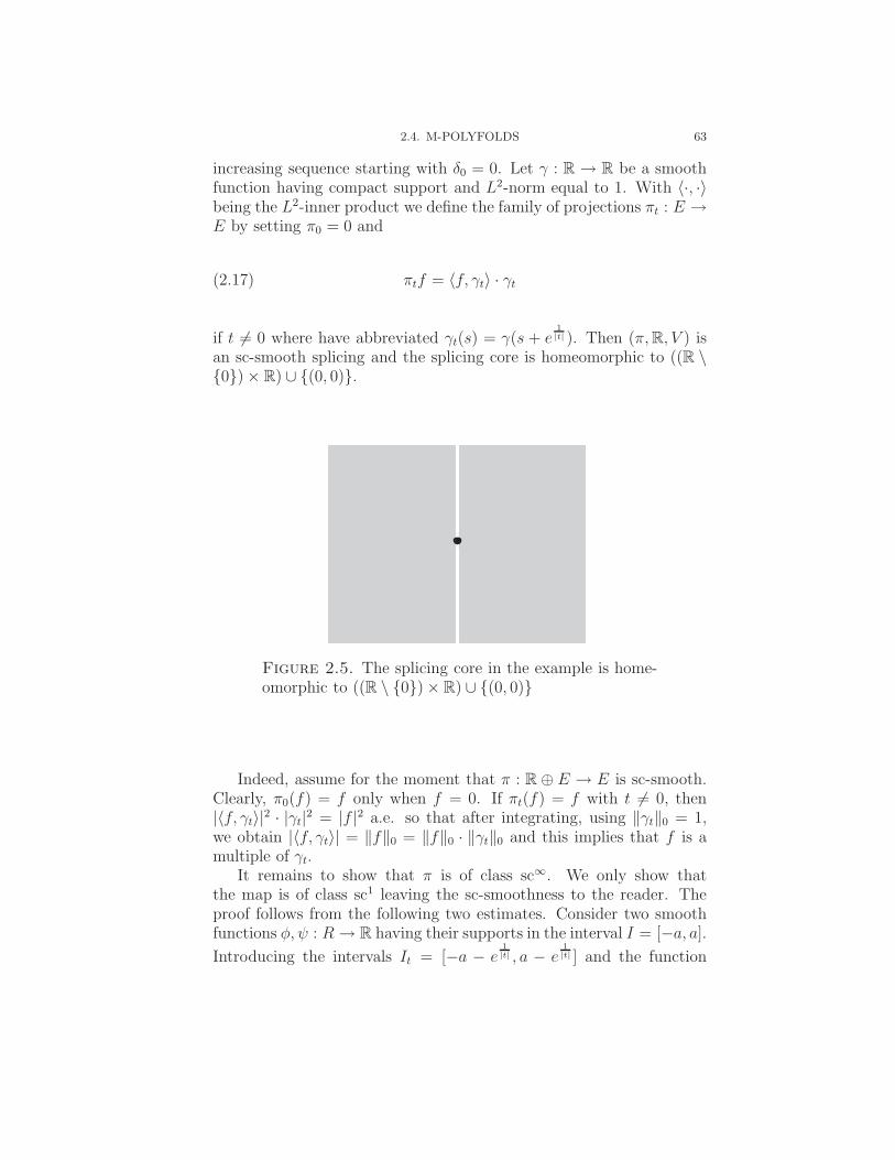
2.4. M-POLYFOLDS 63
increasing sequence starting with δ0 = 0. Let γ : R → R be a smoothfunction having compact support and L2-norm equal to 1. With 〈·, ·〉being the L2-inner product we define the family of projections πt : E →E by setting π0 = 0 and
(2.17) πtf = 〈f, γt〉 · γt
if t �= 0 where have abbreviated γt(s) = γ(s + e1|t| ). Then (π, R, V ) is
an sc-smooth splicing and the splicing core is homeomorphic to ((R \{0}) × R) ∪ {(0, 0)}.
Figure 2.5. The splicing core in the example is home-omorphic to ((R \ {0}) × R) ∪ {(0, 0)}
Indeed, assume for the moment that π : R ⊕ E → E is sc-smooth.Clearly, π0(f) = f only when f = 0. If πt(f) = f with t �= 0, then|〈f, γt〉|
2 · |γt|2 = |f |2 a.e. so that after integrating, using ‖γt‖0 = 1,
we obtain |〈f, γt〉| = ‖f‖0 = ‖f‖0 · ‖γt‖0 and this implies that f is amultiple of γt.
It remains to show that π is of class sc∞. We only show thatthe map is of class sc1 leaving the sc-smoothness to the reader. Theproof follows from the following two estimates. Consider two smoothfunctions φ, ψ : R → R having their supports in the interval I = [−a, a].
Introducing the intervals It = [−a − e1|t| , a − e
1|t| ] and the function

64 2. M-POLYFOLDS
φt(s) = φ(s + e1|t| ), we estimate for f ∈ Em+1,
〈f, φt〉2 =
∫R
|f(s)|2 · |φ(s + e1|t| )|2ds
=
∫It
|f(s)|2 · |φ(s + e1|t| )|2 · e−2δm+1s · e2δm+1sds
≤ Ce−2δm+1e1|t|
· ‖f‖2m+1.
(2.18)
Next we consider the map (t, f) �→ p(t)〈f, φ〉ψt from R ⊕ Em+1 into
Em+1 where p(t) is a polynomial of degree k in variable 1|t|
e1|t| . Using
(2.18) we estimate
‖p(t)〈f, φt〉ψt‖2m = |p(t)〈f, φt〉|
2∑j≤m
∫It
|Djψ(s + e1|t| )|2e2δm|s|ds
≤ |p(t)〈f, φt〉|2∑j≤m
∫I
|Djψ(s)|2e−2δm(s−e1|t| )ds
≤ C|p(t)|2e−2(δm+1−δm)e1|t|‖f‖2
m.
(2.19)
Since δm+1 − δm > 0, the last estimate tends to 0 as t → 0. Withthese two observations we prove our claim. The function γ and henceits derivatives have compact support. If t �= 0 and f ∈ Em+1, then by(2.18),
‖π(t, f)‖m → 0
as t → 0, and since π(0, f) = 0, we conclude that the map π is differ-entiable at the point (0, f) and its derivative is equal to 0. For t �= 0,the derivative dπ(t, f) : R ⊕ Em+1 → Em is given by
dπ(t, f)[δt, δf ] = 〈δf, γt〉γt − sign(t) 1|t|2
e1|t| 〈f, γt〉γt · [δt]
− sign(t) 1|t|2
e1|t| 〈f, γt〉γt · [δt]
where γt denotes the derivative of γt with respect to the variable s.Since the function γ has a compact support we may apply (2.19)to estimate each term. It follows each term tends to 0 in Em ast → 0 showing that the map (t, f) �→ dπ(t, f) from R ⊕ Em+1 intoEm is continuous and the map π : R ⊕ Em+1 → Em is of class C1.Note that, in view of (2.19), the map δf �→ 〈δf, γt〉γt from Em+1
into Em has an extension to a bounded linear map from Em → Em
so that dπ(t, f) : R ⊕ Em+1 → Em has an extension to a linearbounded operator Dπ(t, f) : R ⊕ Em → Em having the property that

2.4. M-POLYFOLDS 65
(t, f, δt, δf) �→ Dπ(t, f)(δt, δf) from R⊕Em+1 ⊕R⊕Em → Em is con-tinuous. In view of Proposition 1.7 we have verified that π : R⊕E → Eis of class sc1.
What is KTS? One can, of course generalize these ideas. For exam-ple, take the open unit disk D◦ in R2 and add a closed interval [−1, 1]and identify the ends ±1 with the points (±1, 0) in the boundary of theclosed disk. A small open disc centered at (±1, 0) intersected with Fig-ure 2.6 (b) is homeomorphic to the splicing core in Figure 2.6 (a). Thesplicing core represented by Figure 2.6 (a) can be obtained by takingE as above and setting πt = 0 for t ≤ 0 and for t > 0 by defining theprojection πt by (2.17). This can be generalized to higher dimensions.
D0
(a) (b)
Figure 2.6
Let us note the following useful result about sc-smooth partitionsof unity.
Theorem 2.14. Let X be an M-polyfold with local models beingsplicing cores build in sc-Hilbert spaces. Assume that (Uλ)λ∈Λ is anopen covering. Then there exists a subordinate sc-smooth partition ofunity (βξ)ξ∈Ξ.
Let us note that the product X × Y of two M-polyfolds is in anatural way a M-polyfold. For charts (U, ϕ,S) and (W, ψ, T ) of X andY , respectively, we define the product chart (U × W, φ × ψ,S ⊕ T ).Here
S × T = (π, V, E) × (ρ, V ′, F ) = (σ, V × V ′, E ⊕ F ),

66 2. M-POLYFOLDS
with
σ(v, v′) = πv ⊕ ρv′ .
We call S × T the product of the splicings. There are several possiblenotions of subpolyfolds (we suppress the M in the notation) and wedescribe them in a later chapter.
2.5. Corners and Boundary points
In this section we will prove the extremely important fact that sc-smooth maps are able to recognize corners. This will be crucial forSFT since most of the algebra is a consequence of the corner structure.
Let X be a M-polyfold. For a point x ∈ X we take a M-polyfoldchart ϕ : U → KS where KS is the splicing core associated withthe splicing S = (π, V, E). Here V is an open subset of a cone Ccontained in an n-dimensional vector space W . By definition thereexists a linear isomorphism from W to Rn mapping C onto [0,∞)n.Identifying the cone C with [0,∞)n ⊂ Rn we shall use the notationϕ = (ϕ1, ϕ2) ∈ [0,∞)n ⊕ E according to the splitting of the targetspace of ϕ. We associate with x ∈ U the integer d(x) defined by
(2.20) d(x) = �{coordinates of ϕ1(x) which are equal to 0}.
Theorem 2.15. The map d : X → N is well-defined and does notdepend on the choice of the compatible polyfold chart. Moreover, everypoint x ∈ X has an open neighborhood O satisfying
d(y) ≤ d(x) for all y ∈ O.
The map d is called the degeneracy index. A point with d(x) = 0is an interior point. A point with d(x) = 1 is called a good boundarypoint. A point with d(x) ≥ 2 is called a corner. In general, d(x) isthe order of the corner .
Proof of Theorem 2.15. Consider two M-polyfold charts ϕ :
U ⊂ X → KS and ϕ′ : U ′ ⊂ X → KS′such that x ∈ U ∩ U ′. In-
troducing the open subsets U = ϕ(U ∩ U ′) and U ′ = ϕ′(U ∩ U ′) ofKSand KS′
resp., and setting ϕ(x) = (r, e) and ϕ′(x) = (r′, e′) wedefine the sc-diffeomorphism Φ : U → U ′ by Φ = ϕ′ ◦ ϕ−1. Obvi-ously, Φ(r, e) = (r′, e′). Now the proof of Theorem 2.15 reduces to thefollowing proposition.
Proposition 2.16. Let S = (π, V, E) and S ′ = (π′, V ′, E ′) be twosplicings having the parameter sets V = [0,∞)k and V ′ = [0,∞)k′
.
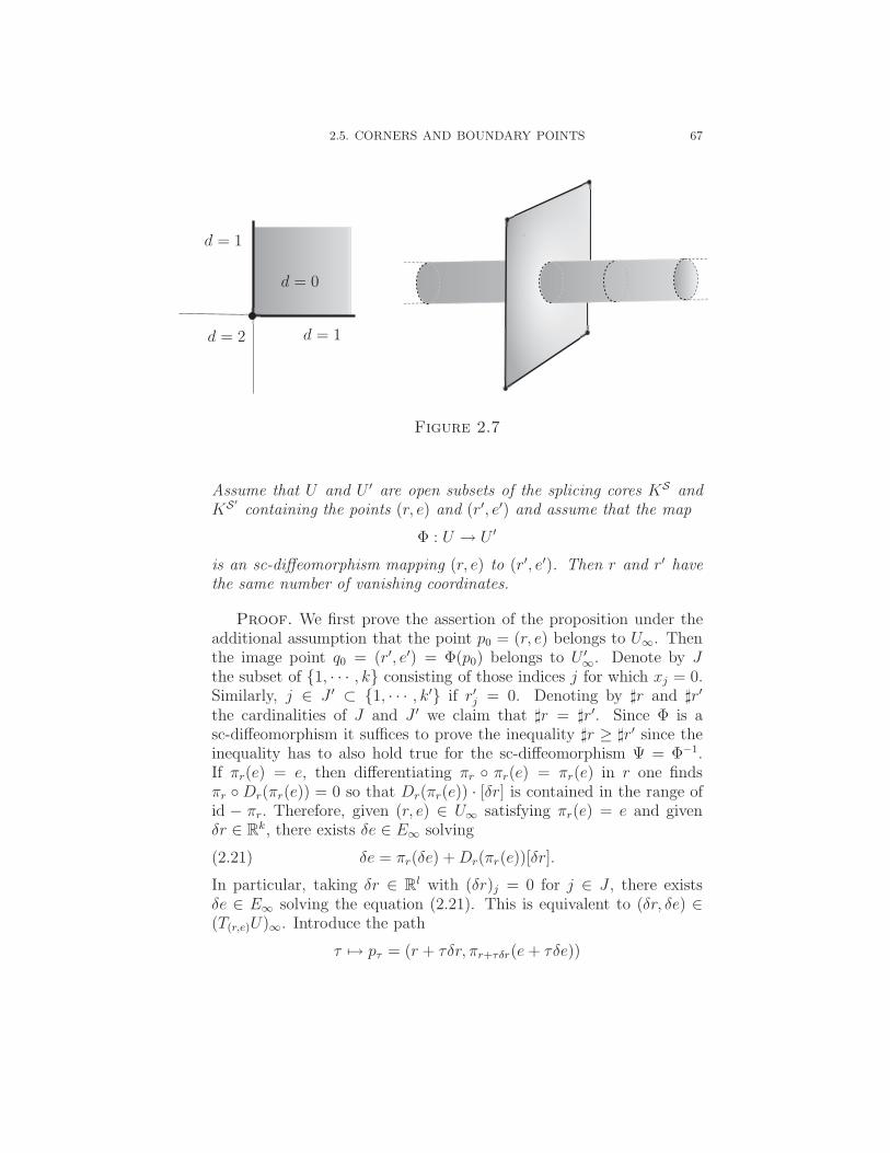
2.5. CORNERS AND BOUNDARY POINTS 67
d = 1
d = 1d = 2
d = 0
Figure 2.7
Assume that U and U ′ are open subsets of the splicing cores KS andKS′
containing the points (r, e) and (r′, e′) and assume that the map
Φ : U → U ′
is an sc-diffeomorphism mapping (r, e) to (r′, e′). Then r and r′ havethe same number of vanishing coordinates.
Proof. We first prove the assertion of the proposition under theadditional assumption that the point p0 = (r, e) belongs to U∞. Thenthe image point q0 = (r′, e′) = Φ(p0) belongs to U ′
∞. Denote by Jthe subset of {1, · · · , k} consisting of those indices j for which xj = 0.Similarly, j ∈ J ′ ⊂ {1, · · · , k′} if r′j = 0. Denoting by �r and �r′
the cardinalities of J and J ′ we claim that �r = �r′. Since Φ is asc-diffeomorphism it suffices to prove the inequality �r ≥ �r′ since theinequality has to also hold true for the sc-diffeomorphism Ψ = Φ−1.If πr(e) = e, then differentiating πr ◦ πr(e) = πr(e) in r one findsπr ◦ Dr(πr(e)) = 0 so that Dr(πr(e)) · [δr] is contained in the range ofid − πr. Therefore, given (r, e) ∈ U∞ satisfying πr(e) = e and givenδr ∈ Rk, there exists δe ∈ E∞ solving
(2.21) δe = πr(δe) + Dr(πr(e))[δr].
In particular, taking δr ∈ Rl with (δr)j = 0 for j ∈ J , there existsδe ∈ E∞ solving the equation (2.21). This is equivalent to (δr, δe) ∈(T(r,e)U)∞. Introduce the path
τ �→ pτ = (r + τδr, πr+τδr(e + τδe))

68 2. M-POLYFOLDS
for |τ | < ρ and ρ small. From (r, e) ∈ U∞ and δe ∈ E∞ one concludespτ ∈ U∞. Moreover, considering τ → pτ as a map into Um for m ≥ 0,its derivative at τ = 0 is equal to (δr, δe). Fix a level m ≥ 1 andconsider the map
(−τ0, τ0) → Rk × Fm : τ → Φ(pτ ).
The map Φ : U → U ′ is C1 as a map from Um+1 ⊂ Rk⊕Em+1 into Rk′⊕
Fm. Its derivative dΦ(r, e) : Rk⊕Em+1 → Rk′⊕Fm has an extension to
the continuous linear operator DΦ(r, e) : Rk ⊕ Em → Rk′⊕ Em. Since
Φ is a sc-diffeomorphism the extension DΦ(r, e) : Rk ⊕Em → Rk′⊕Em
is a bijection. Thus, since δe ∈ E∞,
Φ(pτ ) = Φ(p0) + τ · dΦ(p0)[δr, δe] + om(τ)
= q0 + τ · DΦ(p0)[δr, δe] + om(τ)(2.22)
where om(τ) is a function taking values in Rk′⊕ Fm and satisfying
1τom(τ) → 0 as τ → 0. Introduce the sc-continuous linear functionals
λj : Rk × F → R byλj(s, h) = sj
where j ∈ J ′. Thenλj ◦ Φ(pτ ) ≥ 0
for |τ | < δ0. Applying λj to both sides of (2.22) we conclude for τ > 0
0 ≤1
τ· λj
[Φ(pτ )
]=
1
τ· λj
[Φ(p0) + τ · dΦ(p0)[δr, δe] + om(τ)
]= λj
[DΦ(p0)[δr, δe]
]+ λj
(om(τ)
τ
).
Passing to the limit τ → 0+ we find
0 ≤ λj(DΦ(r, e)[δr, δe])
and replacing (δr, δe) by (−δr,−δe) we obtain the equality sign. Con-sequently,
(2.23) λj(DΨ(r, e)[δr, δe]) = 0, j ∈ J ′
for all [δr, δe] ∈ Rk ⊕ E∞ satisfying πr(e) + Dr(πr(e))[δr] = δe and(δr)i = 0 for all i ∈ J . Introduce the codimension �r subspace L of thetangent splicing core KTS ⊂ Rk ⊕ E∞, defined as
L = {(δr, δr) ∈ Rk ⊕ E∞| πr(δe) + Dr(πr(e))[δr] = δe
and (δr)i = 0 for all i ∈ J }.
Then, in view of (2.23),
DΦ(r, e)L ⊂ {[δr′, δe′] ∈ KTS′
| (δe′)j = 0 for all j ∈ J ′}.

2.5. CORNERS AND BOUNDARY POINTS 69
Because the subspace on the right hand side has codimension �r′ inKTS′
and since DΦ(r, e), being a bijection, maps L onto a codimension�r subspace of KTS′
, it follows that �r′ ≤ �r, as claimed.Next we shall prove the general case. For this we take p0 = (r, e) in
U0, so that the image point (r′, e′) = Φ(r, e) belongs to U ′0. Arguing by
contradiction we may assume without loss of generality that �r > �r′,otherwise we replace Φ by Φ−1. Since U∞ is dense in U0 we find asequence (r, en) ∈ U∞ satisfying πr(en) = en and (r, en) → (r, e) in U0.By the previous discussion �r = �r′n where (r′n, e′n) = Φ(r, en). Since Φis sc-smooth, we have (r′n, e
′n) → (r′, e′) in U ′
0 and π′r′(e
′) = e′. Fromthis convergence we deduce �r′ ≥ �r′n so that �r′ ≥ �r contradicting ourassumption. The proof of Proposition 2.16 is complete. �
To finish the proof of Theorem 2.15 it remains to show that the func-tion d is lower semicontinuous. Arguing indirectly assume that thereexists a sequence of points xk converging to x so that d(xk) > d(x).Since ϕ is continuous, we have the convergence ϕ1(xk) = (rk
1 , · · · , rkn) →
ϕ1(x) = (r1, · · · , rn). If for a given coordinate index j the coordinaterkj = 0 for all but finitely many k, then rj = 0, and if rk
j > 0 for all butfinitely many k, then rj ≥ 0. Hence d(xk) ≤ d(x) contradicting ourassumption. The proof of Theorem 2.15 is complete. �
The results about corner recognition remain true if the projectionsin a splicing are parameterized by open subsets of a partial cone. Re-call that a partial cone P in a finite-dimensional vector space is aclosed subset which by a linear isomorphism to some Rn is mappedonto [0,∞)k × Rn−k. In that case the degeneracy index counts thevanishing of the first k coordinates. These types of parameter sets willarise in SFT. In fact there we will have [0,∞)k × Cl, where the first kcoordinates will be related to the corner structure arising from breakingof trajectories, whereas the other arise from bubbling-off of spheres.
Let us observe that the result about corner recognition allows usto define a degeneracy index d : X → N as follows. Take for a pointx ∈ X a local chart
ϕ : U → KS ⊂ ([0,∞)k × Rn−k) ⊕ E.
Then define d(x) to be the number of the first k coordinates of ϕ(x)which are vanishing. This definition is independent of the choices in-volved. We call d = dX the degeneracy index.
Assume that X × Y is a product of two M-polyfolds. It followsimmediately from the definition of the product structure that
dX×Y (x, y) = dX(x) + dY (y).

70 2. M-POLYFOLDS
If A a subpolyfold of the M-polyfold X then A has an induced degener-acy index dA since it carries an induced M-polyfold structure. ClearlydA ≤ dX |A.
2.6. Appendix II
In this appendix we will prove the important technical Lemma 2.6,which we have used in showing the smoothness of the splicing. For thereader’s convenience we recall the statement of the lemma, which weformulate here as a technical theorem.
Theorem 2.17. Let E = H2(R, Rn) be equipped with the sc-structurewhere level m consists of regularity (m + 2, δm)-maps. Using the expo-nential gluing profile ϕ let R = ϕ(r). Then the following three maps
Γi : [0, 1) ⊕ E → E, i = 1, 2, 3
are sc-smooth.
(a) Let f1 : R → R be a smooth map which is constant outsideof a compact interval so that f1(+∞) = 0. Define Γ1(0, h)(s) =f1(−∞)h(s) and Γ1(r, h)(s) = f1(s −
R2)h(s).
(b) Let f2 : R → R be a smooth map which is constant outside ofa compact interval so that f2(−∞) = 0. Define Γ2(0, h) = 0 andΓ2(r, h)(s) = f2(s −
R2)h(s).
(c) Let f3 : R → R be a compactly supported smooth map and defineΓ3(0, h) = 0 and Γ3(r, h)(s) = f3(s −
R2)h(s − R).
We first observe that the statements (a) and (b) of the theorem areequivalent. Indeed, assuming (a) holds true let f2 be a function asin (b). Define the linear sc-operator L : E → E by h → f2(+∞)h.Clearly, L is sc-smooth. The function f1(s) = f2(s)− f2(+∞) satisfiesthe hypothesis of (a) giving the sc-smooth map Γ1. Since
Γ2(r, h) = Γ1(r, h) + L(h),
(a) implies (b). Similar argument shows that (b) implies (a) provingour claim.
In the following we will prove statements (b) and (c). In the firststep we verify sc0-continuity.
Lemma 2.18. The maps Γ2 and Γ3 are of class sc0.
2.6. APPENDIX II 71
Proof. We begin with Γ2 and consider the induced map [0, 1) ⊕Em → Em. The only difficulty arising could be at r = 0. Thecompactly supported smooth functions are dense in Em. If h0 is acompactly supported smooth function and r > 0 is close to 0, thenΓ3(r, h0) = 0. Now our assertion follows from the observation that thenorm of Γ3(r, ·) : Em → Em is uniformly bounded in r,
‖Γ3(r, h)‖m ≤ C · sup0≤k≤m
‖fk‖C0 · ‖h‖m,
where C is a constant independent of r and u.Next consider the map Γ3. Again the difficulty is at r = 0. For
a compactly supported smooth function h0 and r close to 0 we haveΓ3(r, h0) = 0. Using the density of smooth compactly supported func-tions in Em it suffices to show as before a uniform bound for the op-erator norm of Γ3(r, .) : Em → Em. Assuming supp f2 ⊂ [−a, a] wetake R so large that the interval IR = [−a − R
2, a − R
2] is contained in
(−∞, 0]. Denoting by C a generic constant independent of r and u weestimate
‖Γ3(r, h)‖m ≤ C · ‖h(· − R)eδm·‖Hm(I−R)
≤ C · ‖h · eδm(·+R)‖Hm(IR)
≤ C · eδmR2 · ‖h‖Hm(I−R)
≤ C · ‖h‖m.
The proof of Lemma 2.18 is complete. �
Here are some additional observations which are used in the proofof the theorem.
Lemma 2.19. Let f2 and f3 be as described in the theorem. Ifm, k ≥ 0, we set dm+k,m = 1
2[δm+k − δm] > 0. Then there exists a
constant C = C(m, k) > 0 independent of u and r so that the followingestimates hold true.
‖Γ2(r, u)‖m ≤ C · e−dm+k,m·R · ‖u‖m+k
‖Γ3(r, u)‖m ≤ C · e−dm+k,mR · ‖u‖m+k
for all u ∈ Em+k, where R = ϕ(r).
Proof. We start with the map Γ3. Since supp f3 ⊂ [−a, a], thesupport of the function s �→ f3(s − R
2)u(s − R) is contained in the
interval I−R = [−a + R2, a + R
2]. Denoting by C a generic constant we

72 2. M-POLYFOLDS
estimate
‖f3(· −R2)u(· − R)‖m ≤ C · ‖f2(· −
R2)u(· − R)eδms‖Hm(I−R)
= C · ‖u · eδm(s+R)‖Hm(IR) = C · ‖u · e−δm+kse(δm+δm+k)s+δmR‖Hm+k(IR)
≤ C · e−dm+k,mR · ‖u‖m+k.
To prove the estimate for Γ1 let v ∈ Em+k and assume that thesupport of the function f2 is contained in [−a,∞). Then the supportof the function s → f2(s−
R2)v(s) is contained in [R
2−a,∞). Then one
estimates
‖f2(· −R2)v‖m ≤ C · e−dm+k,m·R · ‖u‖m+k.
The proof of the lemma is complete. �
The following result follows from the sc-smoothness of the R-action.
Lemma 2.20. The maps
R ⊕ E → E
defined by (R, u) → f2(· −R2)u and (R, v) → f3(· −
R2)v(· − R) are
sc-smooth.
Proof. For the first map this is obvious. To see that the secondmap is sc-smooth observe that it can be viewed as the composition ofthe following maps
(R, v) → (R, −R2
∗ v) → (R, f2 · (−R2
∗ v)) → (−R2) ∗ (f2 · (
−R2
∗ v)).
Since each of the above maps is sc-smooth and the composition of sc-smooth maps is sc-smooth the lemma follows. �
We need some estimates for the derivatives of the function
R(r) = e1r − e
which agrees with the gluing profile introduced in (2.6). The nextlemma can be proved by induction.
Lemma 2.21. For every k ≥ 0 there exists a constant Ck > 0 suchthat ∣∣∣∣dkR
dxk(r)
∣∣∣∣ ≤ Ck · R(r) · [ln R(r)]2k
for all r ∈ (0, 12).
Now given two positive integers m and n satisfying m ≥ n considerthe sc-Banach spaces Em = (Em+i)i≥0 and En = (En+i)i≥0. Let f :

2.6. APPENDIX II 73
R → R be a compactly supported smooth function and let k ≥ 0 bean integer. Then we introduce the map
(2.24) A : [0, 12) × Rn × Em → En
by setting A(r, y, u) = 0 if r = 0. If r > 0 we set
A(r, y, u)(s) = y1 · y2 · · · yn · R(r) · Djf(s − R(r)2
) · Diu(s − R(r))
where (y1, . . . , yn) = y ∈ Rn, and
R(r) = Dk1R(r) · Dk2R(r) · · ·DknR(r).
The indices satisfy the conditions m ≥ i + n and k1 + · · ·+ km = k. If
k = 0, we set R(r) = 1. Abbreviating
αk(r) = [R(r)]k · [ln R(r)]2k
one derives from Lemma 2.21 the estimate
(2.25) |R(r)| ≤ C · αk(r).
If k ≥ 0 and d > 0, then clearly,
αk(r) · e−d·R(r) → 0 as r → 0.
The proof of Theorem 2.17 will follow from the next lemma.
Lemma 2.22. The map A viewed as a map from [0, 12)⊕Rn ⊕Em+1
into En is of class C1. At every point (r, y, u) ∈ [0, 12) ⊕ Rn ⊕ Em+1,
the derivative dA(r, y, u) : R ⊕ Rn ⊕ Em+1 → En has an extension tothe bounded linear map DA(r, y, u) : R ⊕ Rn ⊕ Em → En. Moreover,the sc-map A : [0, 1
2) ⊕ Rn ⊕ Em → En is of class sc1. In particular,
the tangent map TA : TEm → TEn,
TA(r, y, u, r, y, u) = (A(r, y, u), DA(r, y, u)[r, y, u])
is of class sc0.
Proof. Since R = ϕ(r) is smooth for r > 0 it follows that A,viewed as a map from [0, 1
2) ⊕ Rn ⊕ Em+1 into En, is continuously
differentiable on the set (0, 12) ⊕ R ⊕ Em+1. We will show that A is
differentiable at every point (0, y, u) and its derivative dA(0, y, u) isequal to 0. In the following we write dm,n = 1
2[δm−δn] which is positive
when m > n.
74 2. M-POLYFOLDS
If (r, y, u) ∈ (0,∞)⊕Rn ⊕Em+1, then we derive from Lemma 2.19and (2.25) the following estimate
‖A(r, y + y, u + u)‖n
= |y1 + y1| · · · |yn + yn| · |R(r)| · ‖Djf(· − R2) · Diu(· − R)‖n
≤ Cαk(r) · e−dm,k+1·R(r) · |y1 + y1| · · · |yn + yn| · ‖u + u‖m+1.
Dividing both sides by |r| + |y| + ‖u‖m+1 and noticing that 1br· αk(r) ·
e−dm,k+1·R(br) → 0 as r → 0 we conclude that
1
|r| + |y| + ‖u‖m+1· ‖A(r, y + y, u + u)‖n → 0
as (r, y, u) → 0 in (0,∞) ⊕ Rn ⊕ Em+1. Recalling that A(0, y, u) = 0our claim follows.
At any other point (r, y, u) with r > 0 the derivative dA(r, y, u) :R⊕Rn ⊕Em+1 → En evaluated at [r, y, u] ∈ R⊕Rn ⊕Em+1 is a linearcombination of the following terms
(1) y1 · · · yl · · · yn · R(r) · Djf(s − R2) · Diu(s − R)
(2) r · y1 · · · yn · DR(r) · Djf(s − R2) · Dui(s − R)
(3) r · y1 · · · yn · R(r) · DR(r) · Dj+1(s − R2) · Diu(s − R)
(4) r · y1 · · · yn · R(r) · DR(r) · Djf(s − R2) · Di+1u(s − R)
(5) y1 · · · yn · R(r) · Djf(s − R2) · Diu(s − R).
Assuming |r|+ |y|+ ‖u‖m+1 ≤ 1 and recalling our notation R(r) =Dk1R(r)·Dk2R(r) · · ·DknR(r) with k1+· · ·+kn = k and the assumptionm ≥ i+n we use Lemma 2.19 and Lemma 2.21 to estimate each of theabove terms and arrive at the following bound,
‖dA(r, y, u)[r, y, u]‖n ≤ C · |R(r)|k+1 · e−dm+1,n·R(r)
· (1 + ‖u‖m+1) ·∑
1≤l≤n
|y1 · y2 · · · yl−1 · (1 + yl) · yl+1 · · · yn|.
In particular, the operator norm of dA(r, y, u) satisfies
‖dA(r, y, u)‖ → 0
as (r, y, u) → (0, z, v) in [0, 12)⊕Rn⊕Em+1. Consequently, the derivative
dA(r, y, u) depends continuously on (r, y, u) ∈ [0, 12) ⊕ Rn ⊕ Em+1 so
that A : [0, 12) ⊕ Rn ⊕ Em+1 → En is of class C1 as claimed.
Next we claim the derivative dA(r, y, u) : R ⊕ Rn ⊕ Em+1 → En atthe point (r, y, u) ∈ [0, 1
2)⊕Rn⊕Em+1 has an extension to a continuous
linear map DA(r, y, u) : R ⊕ Rn ⊕ Em → En. If r = 0, then we setDA(0, y, u) = 0. If r > 0 inspecting the terms (1)-(5) we see that we

2.6. APPENDIX II 75
only have to consider term (5). By Lemma 2.19 and the assumptionm ≥ i + n, term (5) with u ∈ Em can be estimated as follows
‖y1 · y2 · · · yn · R(r) · Djf(· − R2) · Diu(· − R)‖n
≤ |y1| · · · |yn| · |R(r)| · ‖Djf(· − R2) · Diu(· − R)‖n
≤ C · αm(r) · e−[δm−δn]·R(r)
2 · |y1| · · · |yn| · ‖u‖m.
(2.26)
Thus term (5) defines a bounded linear operator in u from Em into En
and so it is also a bounded linear operator from R⊕Rn ⊕Em into En.Therefore, the derivative dA(r, y, u) : R ⊕ Rn ⊕ Em+1 → En has anextension to a continuous linear map DA(r, y, u) : R⊕Rn ⊕Em → En.
In addition, if m > n so that δm − δn > 0, the left hand side of(2.26) converges to 0 as (r, y, u) → (0, z, u0) in [0, 1
2)⊕Rn ⊕Em. In the
case m = n so that i = 0, term (5) has, in view of our convention that
in this case R(r) = 1, the form y1 · · ·yn ·Djf(s− R(r)
2) · u(s−R). Thus
the continuity of the map
(r, y, u) �→ y1 · · · yn · Djf(s − R(r)2
) · u(s − R)
from Rn ⊕ Em → En follows from Lemma 2.18. Since
[0, 12) ⊕ Rn ⊕ Em+1 ⊕ R ⊕ Rn ⊕ Em → En
(r, y, u, r, y, u) �→ DA(r, y, u)[r, y, u]
is a linear combination of maps of the form (1)-(5), it is continuous.Taking l ≥ 1 and (r, y, u, r, y, u) ∈ [0, 1
2) ⊕ Rn ⊕ Em+l+1 ⊕ R ⊕ Rn ⊕
Em+l we observe that DA(r, y, u)[r, y, u] ∈ En+l and it follows from theestimates in Lemma 2.18 and Lemma 2.19 that the evaluation map
[0, 12) ⊕ Rn ⊕ Em+1 ⊕ R ⊕ Rn ⊕ Em → En
(r, y, u, r, y, u) �→ DA(r, y, u)[r, y, u]
is continuous. We have verified that the sc-continuous map A : [0, 12)⊕
Rn⊕Em → En is of class sc1. The finishes the proof of the lemma. �
We are ready to prove Theorem 2.17. We only prove part (c) since theproofs of the two other cases are similar. We drop the subscripts in f3
and Γ3 and simply write f and Γ so that
Γ(r, u)(s) = f(s − R(r)2
) · u(s − R(r)).
We prove the theorem by proving by induction that the followingassertion holds for all positive integers k.
76 2. M-POLYFOLDS
(k) The map Γ : [0, 12)⊕E → E is of class sck and the iterated tangent
map T kΓ : T k([0, 12) ⊕ E) → T kE has the following property. Choose
any factor En of the tangent space T kE and let π be the projection ofT kE onto En. Let (r, y, u) ∈ (T k([0, 1
2) ⊕ E))0 where r ∈ [0, 1
2), y =
(y1, y2, . . . , y2k) ∈ R2k
and u = (u1, u2, . . . u2k) ∈ Em1⊕Em2⊕· · ·⊕Em2k
.
If r = 0, then T kΓ(0, y, u) = 0 and if r > 0, then the compositionπ ◦ T kΓ(r, y, u) is a linear combination of maps having the form
(2.27) yl1 · yl2 · · · yln · R(r) · Djf(s − R(r)2
) · Diul(s − R(r))
where ul ∈ Emland R(r) = Dk1R(r) · Dk2R(r) · · ·DknR(r) and where
the indices satisfy k1 + · · ·+ kn ≤ k and ml ≥ i + n.
We begin with k = 1. We view Γ as a map from [0, 12)⊕E1 into E0.
The map is of class C1 on (0, 12)⊕E1. At the point (r, u) ∈ (0, 1
2)⊕E1
the derivative dΓ(r, u) : R ⊕ E1 → E0 is equal to
dΓ(r, u)[y1, u](s) = −12· y1 · Df(s − R(r)
2) · u(s − R(r))
− y1 · f(s − R(r)2
) · Du(s − R(r))
+ f(s − R(r)2
) · u(s − R(r)).
(2.28)
Notice that each of the three summands has the form of the operatorA in Lemma 2.22. By the proof of Lemma 2.22 we have dΓ(0, u) = 0and the derivative dΓ(r, u) : R⊕E1 → E0 extends to a bounded linearoperator DΓ(r, u) : R ⊕ E0 → E0. In addition, the evaluation map
[0, 12) ⊕ E1 ⊕ R ⊕ E0 → E0
(r, u, y1, u) �→ DΓ(r, u)[y1, u]
is continuous. The same holds true if we consider DΓ(r, u)[y1, u] ∈ El
with (r, u, y1, u) ∈ [0, 12) ⊕ El+1 ⊕ R ⊕ El for every l ≥ 0. Thus, Γ is of
class sc1. The tangent map TΓ : [0, 12) ⊕ E1 ⊕ R ⊕ E → E1 ⊕ E is the
map
TΓ(r, u, y1, u) = (Γ(r, u), DΓ(r, u)[y1, u]).
Taking a projection π of the tangent TE = E1 ⊕ E onto either factor,the composition π◦TΓ(r, u, y1, u) is a linear combination of terms (2.27)in the assertion (k) with k=1. Thus the statement is proved for k = 1.
Next, assuming that the statement (k) with k ≥ 1 holds true, wewill show that the statement (k + 1) also holds true. We start byshowing that the tangent map T kΓ : T k([0, 1
2) ⊕ E) → T kE is of class
sc1. Choose a factor En of the tangent space T kE and let π be the

2.6. APPENDIX II 77
projection of T kE onto En. At a point (r, y, u) ∈ (T k([0, 12) ⊕ E))0 we
have T kΓ(r, y, u) = 0 if r = 0 and otherwise T kΓ(r, y, u) is a linearcombination of maps of the form,
(2.29) yi1 · yl2 · · · yln · R(r) · Djf(s − R(r)2
) · Diul(s − R(r))
where ul ∈ Emland R(r) = Dk1R(r) · Dk2R(r) · · ·DknR(r) and where
the indices satisfy k1 + · · · + kn ≤ k and ml ≥ i + n. Abbrevi-ate u = ul, y1 = yl1, . . . , yn = yln and ml = m. Then, denotingby A(r, y, u) the map defined by (2.29), we conclude from Lemma(2.22) that A is sc1 from the sc-space [0, 1
2) ⊕ Rn ⊕ Eml with the sc-
structure [0, 12)⊕Rn ⊕Eml+α for all integers α ≥ 0 into the sc-Banach
space En equipped with the sc-structure En+α, α ≥ 0. Moreover,DA(0, y, u) = 0. Taking (r, y, u) ∈ (0, 1
2) ⊕ Rn ⊕ Em+1 and evalu-
ating the linear operator DA(r, y, u) : [0, 12) ⊕ Rn ⊕ Em → En at
(r, y, u) ∈ R ⊕ Rn ⊕ Em we see that it is a linear combination ofthe terms (1)-(5) in the proof of Lemma 2.22. Since u ∈ Em+1 andu ∈ Em, the indices in the terms (1)-(3) and (4) satisfy the conditionm+1 > i+n. In the term (5) we have m+1 ≥ (i+1)+n because, byassumption, m ≥ i + n. Since T kΓ is a linear combination of terms ofthe form (2.29) we conclude that T k+1Γ satisfies the conditions of thestatement (k+1). Thus, the statement (k+1) holds true and the proofof Theorem 2.17 is complete. �


CHAPTER 3
The space of curves as an M-Polyfold
For two different points a and b in Rn we have introduced in Sec-tion 1.5 the metric space X(a, b) of parametrized curves u : R → Rn
connecting the point a at −∞ with the point b at +∞. The met-
ric is denoted by d(u, v) = ‖u − v‖. Quotienting out the R-action oftranslation we have obtained the space
X(a, b) = X(a, b)/ ∼
of equivalence classes [u]. Its quotient topology is determined by thecomplete metric d. The space of curves X(a, b) is equipped with ansc-manifold structure.
We now consider three different points a, b and c in Rn and studythe set of curves
(3.1) X = X(a, c) ∪ [X(a, b) × X(b, c)].
We are going to define a second countable paracompact topology on Xwhich induces the previously constructed topology on X(a, c) and onX(a, b) × X(b, c) so that X(a, c) is open and dense in X. After thiswe shall equip the space X with an M-polyfold structure for which thedegeneracy function d introduced in Section 2.5 takes on the valuesd = 0 on X(a, c) and d = 1 on X(a, b) × X(b, c). The polyfold struc-ture on the open subset X(a, c) of X will be induced by the previouslyconstructed sc-manifold structure. Since this particular case explainsall major technical issues we will formulate at the end a situation fre-quently arising in Morse theory.
3.1. The Topology on X
We first introduce some notation. We fix a smooth cut-off functionβ : R → [0, 1] having the properties listed in (2.5), and define for R ≥ 0the cut-off function
τR(s) = β(s − R2).
We shall associate with a pair of parametrized curves (u, v) ∈ X(a, b)×
X(b, c) the glued parametrized curve ⊕R(u, v) ∈ X(a, c) by defining
79

80 3. THE SPACE OF CURVES AS AN M-POLYFOLD
(3.2) ⊕R(u, v)(s) = τR(s) · u(s) + (1 − τR(s)) · v(s − R)
where 0 ≤ R < ∞. If R = ∞ we define
⊕∞(u, v) = (u, v) ∈ X(a, b) × X(b, c).
We have chosen the half line (−∞, 0] as the negative region of R and[0,∞) as the positive region of R for both of our two curves u, v :R → Rn. The gluing is the following procedure. We identify theintervals [0, R] of the positive part [0,∞) of u with interval [−R, 0] ofthe negative part (−∞, 0] of v by s ∈ [0, R] ∼ s′ ∈ [−R, 0] if and onlyif −R + s = s′.
u
v
0
s
s′−R
R
Figure 3.1
From the properties of the cut-off function τR(s) = β(s − R2) one
reads off that
⊕R(u, v)(s) =
{u(s) s ≤ R
2 1
v(s − R) s ≥ R2
+ 1.
We point out the limits as R → ∞,
limR→∞
⊕R(u, v)(s) = u(s)
limR→∞
⊕R(u, v)(s + R) = v(s)
for all s ∈ R.

3.1. THE TOPOLOGY ON X 81
a
b
c
a
b
c
u v
u v
u(0)
u(R) v(−R)
v(0)
⊕R(u, v)
Figure 3.2
We shall use the following notation
[⊕∞(u, v)] := ([u], [v]) ∈ X(a, b) × X(b, c)
where the bracket [u] stands for the equivalence class containing therepresentative u. We use the same formula (3.1) in order to glue thetwo vector fields
s �→ h(s) ∈ Tu(s)Rn = Rn
s′ �→ k(s′) ∈ Tv(s′)Rn = Rn
along the curves u and v, where s ∈ R and s′ ∈ R. We define the vectorfield ⊕R(h, k) along the glued curve ⊕R(u, v) by
⊕R(h, k)(s) = τR(s) · h(s) + (1 − τR(s)) · k(s − R)
for all s ∈ R, where τ(s) = β(s − R2). The identification for the gluing
is as above.In order to keep the information about the vector fields h(s) and
k(s′) also beyond the gluing intervals for s ≥ R and s′ ≤ −R weintroduce the anti-gluing of the vector fields h and k by the formula

82 3. THE SPACE OF CURVES AS AN M-POLYFOLD
h
k
0
s
s′−R
R
0
Figure 3.3
a
b
c
u v0 0
R2
−R2
−RR
Figure 3.4
(3.3) �R(u, v)(s) = −(1 − τR(s)) · u(s) + τR(s) · v(s − R)
for all s ∈ R. Here we use the following identification.In view of properties of the cut-off function β,
⊕R(h, k)(s) =
{h(s) s ≤ R
2− 1
k(s − R) s ≥ R2
+ 1
�R(h, k)(s) =
{k(s − R) s ≤ R
2− 1
−h(s) s ≥ R2
+ 1

3.1. THE TOPOLOGY ON X 83
−hkR
s
s′0
0−R
Figure 3.5
a
b
c
u
v
⊕R(u, v)
Figure 3.6
Next we define the topology of X by defining its basis B. We shalldistinguish between sets of type 1 and sets of type 2 in B. In order to
define a type 1 set we take a path w0 ∈ X(a, c) and a number δ > 0and define the set of curves connecting the point a with the point c by
(3.4) O(w0, δ) = {[w] |w ∈ X(a, c) and d(w0, w) < δ}.

84 3. THE SPACE OF CURVES AS AN M-POLYFOLD
Our notation indicates that we take the representative w0 of [w0]. In
order to define a type 2 set of B we take a pair (u0, v0) ∈ X(a, b) ×
X(b, c) of curves as well as real numbers δ > 0 and R0 > 1 and definethe neighborhood of broken curves (they are broken at R = ∞) as theset
O(u0, v0, R0, δ0) = {[⊕R(u, v)] |(u, v) ∈ X(a, b) × X(b, c)
with d(u0, u) < δ, d(v0, v) < δ and R0 < R ≤ ∞}.
(3.5)
The aim of this section is the proof of the following theorem.
Theorem 3.1. The collection B consisting of sets of type 1 andtype 2 is the basis for a second countable Hausdorff topology for X. Itinduces on the subsets X(a, c) and X(a, b)×X(b, c) the given topology.The subset X(a, c) is open and dense in X.
We start the proof with the following observation.
Lemma 3.2. Fix real numbers t0, t1 and a pair of curves (u, v) ∈
X(a, b) × X(b, c). Then
d(t0 ∗ ⊕R(u, v),⊕R+t1−t0(t0 ∗ u, t1 ∗ v)) → 0
as R → ∞. Moreover,
d([⊕R(u, v)], [⊕R+t1−t0(t0 ∗ u, t1 ∗ v)]) → 0
as R → ∞.
Proof. Abbreviating a = 12[t0 + t1] and R = R′ + (t0 − t1) we
compute
(t0 ∗ ⊕R(u, v))(s) = ⊕R(u, v)(t0 + s)
= τR(t0 + s) · u(t0 + s) + (1 − τR(t0 + s)) · v(t0 + s − R)
= τR′(a + s) · (t0 ∗ u)(s) + (1 − τR′(a + s)) · (t1 ∗ v)(s − R′)
= ⊕R′(t0 ∗ u, t1 ∗ v) + [τR′(a + s) − τR′(s)] · (t0 ∗ u)(s)
− [τR′(a + s) − τR′(s)] · (t1 ∗ v)(s − R′)
=: ⊕R′(t0 ∗ u, t1 ∗ v)(s) + δ(R)(s).
The compact supports of the functions s �→ [τR′(a+s)−τR′ (s)] move to∞ as R → ∞ so that if u and v are fixed, then δ(R) → 0 in H2(R, Rn)

3.1. THE TOPOLOGY ON X 85
as R → ∞. Therefore,
d(t0 ∗ ⊕R(u, v),⊕R′(t0 ∗ u, t1 ∗ v)) → 0
as R → ∞. The second assertion now follows from the inequality
d(α, β) ≤ d(u, v) for any two equivalence classes α, β ∈ X and repre-sentatives u ∈ α, v ∈ β. The proof of the lemma is complete. �
We need the following technical lemmata in which ‖·‖ denotes thenorm on E = H2(R, Rn), and Bδ(0) denotes the open δ-ball around 0in E.
Lemma 3.3. Given ε > 0 there exists δ > 0 so that for every R ≥ 2,
Bδ(0) ⊂ {⊕R(h, k)| ‖h‖, ‖k‖ < ε}.
Proof. Fix u ∈ E and consider the system of equations
⊕R(h, k) = u
�R(h, k) = 0.
The system can be written in the following matrix form[τ(s) 1 − τ(s)
τ(s) − 1 τ(s)
]·
[h(s)
k(s − R)
]=
[u(s)0
].
Multiplying by the inverse matrix we obtain
h(s) =τ(s)
α(s)· u(s)
k(s − R) =1 − τ(s)
α(s)· u(s).
Setting s′ = s − R the last formula takes the form
k(s′) =τ(−s′)
α(−s′)· u(s′ + R).
Using the translation invariance of the norm, we find a constantC > 0 independent of R ≥ 2, depending only on bounds up to thesecond derivatives of the cut off function β, so that ‖h‖+‖k‖ ≤ C ·‖u‖.Consequently, for given ε we may take δ = ε
2Cand our assertion is
proved. �
Lemma 3.4. Given ε > 0 there exists δ > 0 so that for all R ≥ 2,
{⊕R(h, k)| ‖h‖, ‖k‖ < δ} ⊂ Bε(0).
Proof. This follows from a straightforward estimate. �
86 3. THE SPACE OF CURVES AS AN M-POLYFOLD
Next we prove three lemmata which will imply Theorem 3.1
Lemma 3.5. The collection of sets B is the basis for a topology. Theinduced topologies on X(a, c) and X(a, b) × X(b, c) are the previouslydefined ones.
Proof. Assume [w0] ∈ O1 ∩ O′1 where O1, O
′1 are sets of type 1.
Since the type 1 sets are a basis for the topology on X(a, c) we finda set O′′
1 of type 1 so that [w0] ∈ O′′1 ⊂ O1 ∩ O′
1. Next assume that[w0] ∈ O1 ∩ O2, where Oi is of type i. By Lemma 3.3, there existsO′
1 with [w0] ∈ O′1 ⊂ O1 ∩ O2. This also implies that the topology
induced on X(a, c) is the previously defined one. If [w0] belongs toO2∩O′
2 we can pick O1 of type 1 containing [w0] and apply the previousconsideration to O1 ∩O2 and O1 ∩O′
2 in order to find a type 1 set with[w0] ∈ O′
1 ⊂ O2 ∩ O′2. Finally assume that ([u0], [v0]) ∈ O2 ∩ O′
2. Wemay assume without loss of generality that
O2 = O(u0, v0, R0, δ) and O′2 = O(t0 ∗ u0, t1 ∗ v0, R0, δ).
It suffices to show for a suitable S0 >> 0 and a suitable σ > 0 that
O(u0, v0, S0, σ) ⊂ O(t0 ∗ u0, t1 ∗ v0, R0, δ).
Arguing indirectly we find sequences Sk → ∞, uk → u0 and vk → v0
so that
(3.6) [⊕Sk(uk, vk)] �∈ O(t0 ∗ u0, t1 ∗ v0, R0, δ).
We estimate
d(t0 ∗ ⊕Sk(uk, vk),⊕Sk+t1−t0(t0 ∗ uk, t1 ∗ vk))
≤ d(t0 ∗ ⊕Sk(uk, vk), t0 ∗ ⊕Sk
(u0, v0))
+ d(t0 ∗ ⊕Sk(u0, v0),⊕Sk+t1−t0(t0 ∗ u0, t1 ∗ v0))
+ d(⊕Sk+t1−t0(t0 ∗ u0, t1 ∗ v0),⊕Sk+t1−t0(t0 ∗ uk, t1 ∗ vk))
= ‖t0 ∗ ⊕Sk(uk − u0, vk − v0)‖
+ ‖⊕Sk+t1−t0(t0 ∗ (uk − u0), t1 ∗ (vk − v0))‖
+ d(t0 ∗ ⊕Sk(u0, v0),⊕Sk+t1−t0(t0 ∗ u0, t1 ∗ v0))
=: Ik + IIk + IIIk.
Using the invariance of the norm under the R-action and Lemma 3.4one sees that Ik → 0. Lemma 3.4 also implies IIk → 0 and fromLemma 3.2 one deduces IIIk → 0. Therefore,
d(t0 ∗ ⊕Sk(uk, vk),⊕Sk+t1−t0(t0 ∗ uk, t1 ∗ vk)) → 0

3.1. THE TOPOLOGY ON X 87
as k → ∞. Using Lemma 3.3 we find σ > 0 so that
Bσ(0) ⊂ ⊕R(Bδ/2(0), Bδ/2(0))
for all R ≥ 2. For large k the element t0 ∗ ⊕Sk(uk, vk) belongs to
⊕Sk+t1−t0(t0∗uk, t1∗vk)+Bσ(0) which in turn belongs to ⊕Sk+t1−t0(Bδ(t0∗u0), Bδ(t1 ∗ v0)). Now passing to equivalence classes we conclude
[⊕Sk(uk, vk)] ∈ O(t0 ∗ u0, t1 ∗ v0, R0, δ),
contradicting (3.6). This shows that B is a basis for a topology. Fromthe form of the sets of type 2 in (3.5) one reads off immediately thatthe induced topology on X(a, b)×X(b, c) is the previously defined one.The proof of Lemma 3.5 is complete. �
Lemma 3.6. The topology generated by B is Hausdorff.
Proof. Arguing by contradiction we assume the points ([u0], [v0])and ([a0], [b0]) in X(a, b)×X(b, c) do not have disjoint neighborhoods.Then there are sequences Sk and Rk → ∞, tk ∈ R and (uk, vk) →(u0, v0) and (ak, bk) → (a0, b0) such that
tk ∗ ⊕Rk(uk, vk) = ⊕Sk
(ak, bk).
of Lemma 3.4 this implies that
(3.7) tk ∗ ⊕Rk(u0, v0) −⊕Sk
(a0, b0) → 0
in E = H2(R, Rn). From Sk → ∞ we deduce ⊕Sk(a0, b0)(s) → a0(s) as
k → ∞ for every s ∈ R. We claim that the sequence tk is bounded. Ifnot we assume first that tk → −∞. Then for every fixed s,
tk ∗ ⊕Rk(u0, v0)(s) = u0(s + tk) → a
as k → ∞. Hence a = a0(s) for all s, contradicting a0(s) → b �= a ass → ∞. If tk → ∞, then at s − tk with k large,
tk ∗ ⊕Rk(u0, v0)(s − tk) = u0(s)
while⊕Sk
(a0, b0)(s − tk) = a0(s − tk) → a.
This implies u0(s) = a for all s ∈ R contradicting u0(s) → b �= aas s → ∞. Thus the sequence tk is bounded and we may assumetk → t0. We next claim that the sequence Rk −Sk is bounded. Indeed,if Rk − Sk → ∞, then for fixed s as k → ∞
tk ⊕Rk(u0, v0)(s + Rk) = u0(s + tk + Rk) → b
while⊕Sk
(a0, b0)(s + Rk) = b0(s + (Rk − Sk)) → c �= b,

88 3. THE SPACE OF CURVES AS AN M-POLYFOLD
contradicting (3.7). If Rk − Sk → −∞, then
tk ⊕Rk(u0, v0)(s + Sk) = v0(s + tk + (Sk − Rk)) → c
while⊕Sk
(a0, b0)(s + Sk) = b0(s).
Hence b0(s) = c. But this contradicts b0(s) → b �= c as s → ∞.Thus the sequence Rk − Sk is bounded and we may assume that itconverges to τ . Then evaluating tk ⊕Rk
(u0, v0) and ⊕Sk(a0, b0) at s
and passing to the limit as k → ∞ we find t0 ∗ u0 = a0. Evaluatingboth sequences at s + Rk we conclude
tk ⊕Rk(u0, v0)(s + Rk) = v0(s + tk) → t0 ∗ v0(s)
and⊕Sk
(a0, b0)(s + Rk) = b0(s + (Rk − Sk)) → τ ∗ b0(s).
Hence ([u0], [v0]) = ([a0], [b0]) contradicting our assumption that thesepoints are different.
If we have two different points [w0] �= [w′0] in X(a, c), the existence
of separating open neighborhoods is immediate. The remaining casewhere the points [w0] ∈ X(a, c) and ([u0], [v0]) ∈ X(a, b) × X(b, c) canbe separated by open sets is left to the reader. �
Lemma 3.7. The topology generated by B on X is second countable.
Proof. Recall from Section 1.5 that X(a, c) is second countable.Take a countable basis for its topology, say Wi for i ≥ 1. We also know
that X(a, b) and X(b, c) are second countable. Take a countable basisUi for the first and a countable basis Vj for the second space. Definethe subsets Oi,j,k of X by
Oi,j,k = {[⊕R(u, v)] | u ∈ Ui v ∈ Vj , R ∈ (k,∞]}.
This collection of sets is a countable basis on X. �
In view of Lemmata 3.5, 3.6 and 3.7 the proof of Theorem 3.1 iscomplete. �
We would like to point out that the definition of B does not depend onthe choice of the cut-off function β used in all our constructions.
3.2. M-Polyfold Charts on X
In this section we will construct a M-polyfold structure on X. Forpoints in X(a, c) we can take the sc-charts with domains disjoint fromX(a, b)×X(b, c) which we constructed in Section 1.5. Clearly sc-chartsare also M-polyfold charts the splicing being defined by V = {0} and

3.2. M-POLYFOLD CHARTS ON X 89
π0 = Id so that the splicing core is {0} ⊕ E = E. Before constructingM-polyfold charts for points in X(a, b)×X(b, c) we have to recall somefacts from Section 1.5.
If a pair ([u′], [v′]) ∈ X(a, b)×X(b, c) is given, then there are positivenumbers ε and ε1 and a pair ([u], [v]) ∈ X(a, b)×X(b, c) having smooth
representatives (u, v) ∈ X(a, b) × X(b, c) and satisfying
(3.8)‖u − u′‖C0(R) < ε1 and ‖u − u′‖C1([−ε,ε]) < ε2
‖v − v′‖C0(R) < ε1 and ‖v − v′‖C1([−ε,ε]) < ε2.
In addition, there are affine hyperplanes Σu and Σv in Rn so that uintersects Σu and v intersects Σv transversally at the parameter values = 0. Moreover, considering parametrized paths nearby we take h, k ∈E satisfying the estimates
(3.9) ‖h‖C1([−ε,ε]) < ε2 and ‖k‖C1([−ε,ε]) < ε2.
Then the paths u +h ∈ X(a, b) resp. v + k ∈ X(b, c) intersect Σu resp.Σv transversally at unique points parametrized by s satisfying |s| < ε.In addition, there exist positive numbers α and ε2 such that if
‖h‖C0(R), ‖h′‖C0(R), ‖k‖C0(R), ‖k‖C0(R) < ε2
and
(3.10) u + h = t ∗ (u + h′) and v + k = t′ ∗ (v + k′)
on [−α, α] for some t, t′ ∈ R, then necessarily |t|, |t′| < ε. Recall fur-thermore the following construction of an sc-chart at [u] ∈ X(a, b).Introduce the closed subspace Fu ⊂ E consisting of functions h satis-fying h(0) ∈ Σu − u(0). Define the open subset U of Fu by
(3.11) U = {h ∈ Fu | ‖h‖C0(R) < ε1 and ‖h‖C1([−ε,ε]) < ε2}.
Then the map
U → X(a, b)
h �→ [u + h]
defines an sc-chart. It should be recalled that E is the Banach spaceE = H2(R, Rn) equipped with the sc-smooth structure introduced inSection 1.5.
Similarly, an sc chart at [v] ∈ X(b, c) is defined by the map
V → X(b, c)
k �→ [v + k]
from the open subset V ⊆ Fv defined by

90 3. THE SPACE OF CURVES AS AN M-POLYFOLD
(3.12) V = {h ∈ Fv | ‖k‖C0(R) < ε1 and ‖k‖C1([−ε,ε]) < ε2}
where the subspace Fv consists of functions k in E satisfying k(0) ∈Σv − v(0).
Lemma 3.8. Let the data be as just described. Then there exists areal number R0 > 2 so that for R, R′ ≥ R0, for h, h′ ∈ U and k, k′ ∈ Vand t ∈ R, the equality
(3.13) ⊕R(u + h, v + k) = t ∗ ⊕R′(u + h′, v + k′)
implies t = 0 and R = R′.
Proof. We choose R0 = 2α + 2 with α as in (3.10) . Pick R, R′ ≥R0 and assume
⊕R(u + h, v + k) = t ∗ ⊕R′(u + h′, v + k′)
for some r ∈ R. We may assume t ≤ 0, interchanging if necessary theroles of (h, k) and (h′, k′). In view of the choice of R0 and since thefunction τR is equal to 1 for s ≤ R
2− 1, it follows from (3.13) that
(u + h)(s) = (u + h′)(t + s) = (t ∗ (u + h′))(s)
for all s ∈ [−α, α]. Thus (3.10) implies |t| < ε. Setting s = 0 andrecalling that h ∈ Fu − u(0) we obtain u(0) + h(0) = u(t) + h′(t) ∈ Σu.Since h′ ∈ Fu we also know u(0) + h′(0) ∈ Σu and conclude t = 0 fromthe uniqueness of the intersection under assumption (3.9). Hence
⊕R(u + h, v + k) = ⊕R′(u + h′, v + k′)
and we will show that R = R′. We may assume R ≥ R′. Evaluatingthe above paths at s + R with s ∈ [−α, α] we find
(v + h)(s) = (v + h′)(s − R′ + R) = (R − R′) ∗ (v + h′)(s)
if s ∈ [−α, α]. Again applying 3.10 we conclude R = R′. The proof iscomplete. �
Choose R0 = 2α+2 as in Lemma 3.8. If r0 ∈ (0, 1) satisfies ϕ(r0) > R0,
where ϕ is the gluing profile ϕ(r) = e1r − e, we define the gluing map
(3.14) A : [0, r0) ⊕ U ⊕ V → X
for r = 0 by
A(0, h, k) = ([u + h], [v + k])

3.2. M-POLYFOLD CHARTS ON X 91
and if r ∈ (0, r0), we put
A(r, h, k) = [⊕R(u + h, v + k)]
where R = ϕ(r). By construction, the map A is continuous.
Lemma 3.9. If
A(r, h, k) = A(r′, h′, k′)
and �R(h, k) = 0 and �R′(h′, k′) = 0 where R = ϕ(r) and R′ = ϕ(r′),then (r, h, k) = (r′, h′, k′).
Proof. If A(r, h, k) = A(r′, h′, k′) and one of the two numbers r, r′
vanishes, then the other vanishes as well. If r = r′ = 0, then
([u + h], [v + k]) = ([u + h′], [v + k′])
for h, h′ ∈ U and k, k′ ∈ V , implying h = h′ and k = k′ because the datadefine charts for X(a, b) and X(b, c). Now assume r, r′ ∈ (0, r0). FromA(r, h, k) = A(r′, h′, k′) we conclude the existence of t ∈ R satisfying
(3.15) ⊕R(u + h, v + k) = t ∗ ⊕R′(u + h′, v + k′).
Here R = ϕ(r), R′ = ϕ(r′) and, by construction, R > R0 and R′ > R0.Hence t = 0 and R = R′ in view of Lemma 3.8, so that
⊕R(u + h, v + k) = ⊕R(u + h′, v + k′)
implying
⊕R(h, k) = ⊕R(h′, k′).
This together with �R(h, k) = �R(h′, k′) = 0 imply (h, k) = (h′, k′).The proof of the lemma is complete. �
Define the splicing
S = (π, Fu ⊕ Fv, [0, r0))
as in Section 2.2 by the formulae in (2.8) replacing E+ by Fu and E−
by Fv. The formulae (2.8) holds true this time for all s ∈ R and all
s′ ∈ R. Hence, if (h, k) ∈ Fu ⊕ Fv, then πr(h, k) = (h, k) ∈ Fu ⊕ Fv isdefined by the formulae
h(s) =τ(s)
α(s)
[τ(s) · h(s) + (1 − τ(s)) · k(s − R)
]k(s′) =
τ(−s′)
α(−s′)
[(1 − τ(−s′)) · h(s′ + R) + τ(−s′) · k(s′)
]

92 3. THE SPACE OF CURVES AS AN M-POLYFOLD
for all s ∈ R and s′ ∈ R. Near 0 the functions are not changed,
(3.16)
h(s) =
{h(s) 0 ≤ s ≤ R
2− 1
0 s ≥ R2
+ 1
k(s′) =
{0 s′ ≤ −R
2− 1
k(s′) s′ ≥ −R2
+ 1.
The associated splicing core KS is characterized as the collection ofpoints (r, h, k) ∈ [0, r0) ⊕ Fu ⊕ Fv satisfying �R(h, k) = 0 where R =ϕ(r). Take the open set O of the splicing core KS defined by
O = ([0, r0) ⊕ U ⊕ V ) ∩ KS
with U and V according to (3.11) and (3.12). In view of Lemma 3.9,the map
(3.17) A : O → X
is injective.
Lemma 3.10. The map A : O → X is a homeomorphism onto someopen subset of X.
Proof. We already know that A is continuous and injective. Itremains to show that A is open. Take an open subset O′ of O. We willshow that every point of A(O′) is an interior point of A(O). Assumefirst that for (r, h, k) ∈ O′, the image point A(r, h, k) belongs to X(a, c).Taking the representative w of A(r, h, k) we have the path
(3.18) ⊕R(u + h, v + k) = w ∈ X(a, c).
Here R = ϕ(r) with r ∈ (0, r0) and the pair (h, k) ∈ U ⊕ V satisfiesπr(h, k) = (h, k) or equivalently �R(h, k) = 0. Evaluating both sidesof (3.18) at 0 and R we conclude from the definition of the sets U andV that
w(0) = (u + h)(0) ∈ Σu and w(R) = (v + k)(0) ∈ Σv.
It follows from the implicit function theorem, arguing as in Lemma(1.30), that if g ∈ E is close to 0 in E, then there exists a unique timet0(g) so that (w + g)(t0(g)) ∈ Σu. The map g �→ t0(g) is sc-smooth andt0(0) = 0. Similarly, there exists a sc-smooth map g �→ t1(g) satisfyingt1(0) = R and (w + g)(t1(g)) ∈ Σv. Set R′ = t1(g)− t0(g) and define r′
via R′ = ϕ(r′).

3.2. M-POLYFOLD CHARTS ON X 93
We look for the pair (h′, k′) ∈ U × V solving the following twoequations for given g ∈ E close to 0
⊕R′(h′, k′) = t0(g) ∗ (w + g) −⊕R′(u, v) and �R′ (h′, k′) = 0.
Abbreviating the functions τ ′ = β(· − R′
2) and α′ = (τ ′)2 + (1 − τ ′)2,
the solution (h′, k′) can be written explicitly as
[h′(s)
k′(s − R′)
]=
1
α′
[τ ′ −(1 − τ ′)
1 − τ ′ τ ′
]·
[t0(g) ∗ (w + g) −⊕R′(u, v)
0
].
It follows immediately that if g ∈ E is close to 0 in E then (r′, h′, k′)is close to (r, h, k) in R⊕E ⊕E. The condition �R′(h′, k′) = 0 implies(h′, k′) ∈ KS . Substituting s = 0 and then s = R in the above equationwe find
h′(0) = (w + g)(t0(g)) − u(0) ∈ Σu − u(0) = Fu
k′(0) = (w + g)(t1(g)) − v(0) ∈ Σv − v(0) = Fv.
Summing up, we have proved for every g ∈ E near 0 in E that thereexists (r′, h′, k′) ∈ O′ satisfying A(r′, h′, k′) = [w + g]. Thus A(r, h, k)is an interior point of A(O′).
Next we consider the case ([u0], [v0]) ∈ A(O′). In view of the defi-nition of A we have A(0, h0, k0) = ([u0], [v0]) for some (h0, k0) ∈ U ⊕V .Taking representatives we may assume u0 = u+h0 and v0 = v+k0. Re-call that by construction of the topology on X, an open neighborhoodof ([u0], [v0]) consists of the set of equivalence classes [⊕R(u0+h, v0+k)]where R is large including +∞ and h and k are close to 0 in E. Us-ing the implicit function theorem as above we find sc-smooth functionsh �→ t0(h) and k �→ t1(k) defined for h and k close to 0 in E such thatt0(0) = 0 and t1(0) = 0 and
(u0 + h)(t0(h)) ∈ Σu and (v0 + k)(t1(k)) ∈ Σv.
Introduce the path
w := t0(h) ∗ ⊕R(u0 + h, v0 + k) ∈ X(a, c).
Obviously, [w] = [⊕R(u0 + h, v0 + k)]. Taking R large and settingR′ = R + [t1(k) − t0(h)] we deduce from the definition of w that
w(0) = (u0 + h)(t0(h)) ∈ Σu and w(R′) = (v0 + k)(t1(k)) ∈ Σv.
Now we look for solutions (h′, k′) of the equations
⊕R′(h′, k′) = w −⊕R′(u, v) and �R′ (h′, k′) = 0.

94 3. THE SPACE OF CURVES AS AN M-POLYFOLD
Explicitly, the solution (h′, k′) is given by[h′(s)
k′(s − R′)
]=
1
α′
[τ ′ −(1 − τ ′)
1 − τ ′ τ ′
]·
[w −⊕R′(u, v)
0
]where as before τ ′ = β(· − R′
2) and α′ = (τ ′)2 + (1 − τ ′)2. It follows
for R large and hence for R′ large that the resulting solution (h′, k′) isclose to (h0, k0) in E⊕E. Moreover, (h′, k′) ∈ KS since �R′(h′, k′) = 0.Furthermore, substituting s = 0 and s = R′ into the the above equationwe find
h′(0) = w(0) − u(0) ∈ Σu − u(0) = Fu
and k′(0) ∈ Fv. Hence taking R large and defining r′ via R′ = ϕ(r′) weconclude (r′, h′, k′) ∈ O′ and A(r′, h′, k′) = [⊕R′(u + h′, v + k′)] = [w]showing that ([u0], [v0]) is an interior point of A(O′). Thus the map Ais open and the proof of the lemma is complete. �
This implies the following result.
Lemma 3.11. The topological space X is a second countable metriz-able space.
Proof. We already know from Theorem 3.1 that the space X issecond countable and Hausdorff. Since by Lemma 3.10 X is locallyhomeomorphic to open sets in splicing cores, we know that it is com-pletely regular which implies also assertion by Proposition 1.25. �
In view of Lemma 3.10, the map A : O → X defined by (3.17) isa homeomorphism onto an open subset A(O) of the topological spaceX. Abbreviating this open set by
U = A(O) ⊂ X
we denote by
Φ := A−1 : U → O
the inverse of the map A. Then the collection of all charts (U, Φ) ormore precisely (U, Φ, (O,S)), as well as the previously constructed sc-charts for X(a, c), have the property that the union of their domainscovers X. Our main result in this section is the following theorem.
Theorem 3.12. The atlas consisting of all sc-charts for X(a, c)and all charts (U, Φ, (O,S)) around smooth points in X(a, b)×X(b, c)covers X and the transition maps are sc-smooth. In other words theatlas defines a sc-smooth M-polyfold structure.

3.2. M-POLYFOLD CHARTS ON X 95
Proof. Recall that we distinguish between the charts of type 1which are inherited from X(a, c) and charts of type 2 which involve thegluing construction. We already have proved in Lemma 1.33 that thetransition maps between two charts of type 1 are sc-smooth.
We now consider the transition maps from charts of type 1 to chartsof type 2. Take a chart Φ1 : U1 → O1 of type 1 and a chart Φ2 : U2 → O2
of type 2. Then A1 = Φ−11 : O1 → U1 and A2 = Φ−1
2 : O2 → U2.Assuming that the domain of A−2
2 ◦ A1 is nonempty we will show thatit is sc-smooth. Assume A1(f0) = A(r0, h0, k0) for some f0 ∈ O1 and
(r0, h0, k0) ∈ O2 ⊂ KS . Then there are curves u ∈ X(a, b) and v ∈
X(b, c) and w ∈ X(a, c) and real numbers R0 ≥ 2 and t0 ∈ R satisfying
⊕R0(u + h0, v + k0) = t0 ∗ (w + f0)
where R0 = ϕ(r0). In addition, �R0(h0, k0) = 0 since (h0, k0) ∈ KS .In view of the definition of O2 the functions h0 and k0 belong to the
spaces Fu and Fv, respectively, from which we conclude after evaluatingthe above equation at 0 and R0 that (u + h0)(0) = (w + f0)(t0) ∈ Σu
and (v + k0)(0) = (w + f0)(R0 + t0) ∈ Σv. Using the implicit functiontheorem we find two sc-smooth functions f �→ t0(f) and f �→ t1(f)defined for f close to f0 in E satisfying
(w + f)(t0(f)) ∈ Σu and (w + f)(R0 + t1(f)) ∈ Σv,
moreover, t0(f0) = t0 and t1(f0) = t0. Define the positive numberR(f) = R0 + [t1(f) − t0(f)]. Then the curve t0(f) ∗ (w + f) intersectsΣu and Σv at the times 0 and R(f). We define r(f) via the formula
(3.19) R(f) = ϕ(r(f)).
We look for a pair (h, k) solving the following two equations
⊕R(f)(h, k) = t0(f) ∗ (w + f) −⊕R(f)(u, v) and �R(f) (h, k) = 0.
Introducing wR(f) := t0(f) ∗ (w + f) − ⊕R(f)(u, v), the solution pair(h, k) can be represented explicitly as[
h(s)k(s − R(f))
]=
1
α(f)
[τ(f) −(1 − τ(f))
(1 − τ(f)) τ(f)
]·
[wR(f)
0
]where we have abbreviated τ(f) = β(·− R(f)
2) and α(f) = τ(f)2 +(1−
τ(f))2. We denote the solution as (h(f), k(f)). We only consider h(f)since the results for k(f) are proved in a similar way. We set
γ(f) =τ(f)
α(f).

96 3. THE SPACE OF CURVES AS AN M-POLYFOLD
and define the map
(3.20) f �→ h(f) = γ(f) ·[t0(f) ∗ (w + f) −⊕R(f)(u, v)
]from E into E.
Lemma 3.13. The map (3.20) is sc-smooth.
Proof. The curves u ∈ X(a, b), v ∈ X(b, c) and w ∈ X(a, c) havethe form u = φ+h′
0, v = ψ+k′0 and w = η+g′
0 where h′0, k
′0 and g′
0 ∈ Eand φ, ψ and η are smooth functions which are constant outside theinterval [−1, 1]. We represent the map under consideration as a sum,
γ(f) ·[t0(f) ∗ (w + f) −⊕R(u, v)
]= γ(f) · t0(f) ∗ f
+ γ(f) · t0(f) ∗ g′0 − γ(f) · ⊕R(f)(h
′0, k
′0)
+ γ(f) · [t0(f) ∗ η −⊕R(f)(φ, ψ)].
(3.21)
The sc-smoothness of the first two maps follows from the sc-smoothnessof the R-action together with Theorem 2.17. The third map is equalto
γ(f) · τR(f)h′0 + γ(f) · (1 − τR(f)) · k
′0(· − R(f)).
Sc-smoothness follows by applying Theorem 2.17 to each of the abovesummands. Finally, the last term can be represented as
γ(f) · [t0(f) ∗ η −⊕R(f)(φ, ψ)]
= γ(f) · τR(f) · [t0(f) ∗ η(s) − φ(s)]
+ γ(f) · (1 − τR(f)) · [t0(f) ∗ η(s) − ψ(s − R(f))].
(3.22)
The maps f �→ t0(f) and f �→ t1(f) are bounded, hence, R(f) =R0 + [t1(f) − t0(f)] is also bounded. Since φ(s) = η(s) = a for s ≤ −1and φ(s) = b and η(s) = c for s ≥ 1, the first map on the right handside can be written as
γ(f) · τR(f) · [t0(f) ∗ η − φ] = γ(f) · τR(f) · β(· − C) · [t0(f) ∗ η − φ]
where C is a large positive constant.Let δ : R → E be the map defined by δ(x) = β(·−C)·[η(·−x)−φ(·)].
Since δ is sc-smooth, the composition f �→ δ(t0(f)) from E into E isalso sc-smooth. Define the function γ by
(3.23) γ(s) =β(s)
β(s)2 + (1 − β(s))2,
where β is the cut-off function from (2.5). With the function γ = γ · βhaving its support in (−∞, 1], the map Γ(r, g) = γ(· − R
2) · g for g ∈ E

3.2. M-POLYFOLD CHARTS ON X 97
is sc-smooth by Theorem 2.17. Thus, the composition
f −−→ (R(f), t0(f))(ϕ−1,δ)
−−−−−→ (r(f), δ(t0(f))Γ
−−→ Γ(r(f), δ(t0(f)))
is sc-smooth. The first term on the right hand side of (3.22) is preciselythis composition and so it defines an sc-smooth map.
In view of the boundedness of the maps f �→ t0(f) and f �→ t1(f),and hence also of R(f) = R0 +[t1(f)− t0(f)], the second term from onthe right hand side of (3.22) can be written as
γ(f)·(1 − τR(f)) · [t0(f) ∗ η(s) − ψ(s − R(f))]
= γ(f) · (1 − τR(f)) · β(s − C) · [t0(f) ∗ η(s) − ψ(s − R(f))]
where C is a large positive constant C.The map ξ from R2 to E defined by ξ(x, y) = β(· −C) · [η(·+ x)−
ψ(· − y) is sc-smooth implying that f �→ ξ(t0(f), R(f)) is also of classsc∞.
The function γ = γ · (1−β) has a compact support so that, in viewof Theorem 2.17, the map Γ1(r, g) := γ(· − R
2) · g is sc-smooth. Thus,
the composition,
f −−→ (R(f), t0(f))(ϕ−1,ξ)
−−−−−→(r(f), ξ(R(f), t0(f))
Γ1−−−→ Γ1[r(f), ξ(R(f), t0(f))]
is sc-smooth. The second term of (3.22) is precisely the above compo-sition and so the proof of the lemma is complete. �
The lemma holds also true for the map f �→ k(f). Since the tran-sition map A−2
2 ◦ A1 is given by f �→ (h(f), k(f)) we conclude thatA−2
2 ◦ A1 is sc-smooth.
We next consider the transition map A−11 ◦ A2. Assume that A1(f0) =
A2(r0, h0, k0) for some f0 ∈ O1 and for (r0, h0, k0) ∈ O2 ⊂ KS with
r0 > 0. Then there are curves u ∈ X(a, b) and v ∈ X(b, c) and
w ∈ X(a, c) and a real number t0 satisfying
(3.24) t0 ∗ ⊕R0(u + h0, v + k0) = w + f0
where R0 = ϕ(r0). Evaluating both sides at time s = 0 we find
⊕R0(u + h0, v + k0)(t0) = (w + f0)(0) ∈ Σw.

98 3. THE SPACE OF CURVES AS AN M-POLYFOLD
Lemma 3.14. There exists an sc-smooth map (R, h, k) �→ t(R, h, k)defined for R, h and k close to R0, h0 and k0 respectively so that atthe parameter value t(R, h, k) the curve ⊕R(u + h, v + k) intersects Σw
transversally and satisfies, in addition, t(R0, h0, k0) = t0.
Proof. To see this we proceed as in Lemma 1.30 and representΣ := Σw as Σ = {x ∈ Rn| λ(x) = c} for some linear map λ : Rn → Rand some constant c ∈ R, and define the map F : R⊕(0,∞)⊕E⊕E →R by setting
F (t, R, h, k) = λ(⊕R(u + h, v + k)(t + t0)) − c.(3.25)
At the point (0, R0, h0, k0) we have F (0, R0, h0, k0) = 0. Because of theSobolev embedding E ⊂ C1(R) the map F is of class C1. From (3.24)we conclude that the derivative of F with respect to t at the point(0, R0, h0, k0) is equal to
dtF (0, R0, h0, k0)[δt] = λ(w′(0) + f ′0(0)) · [δt]
for all δt ∈ R. Since the curve w + f0 intersects Σ transversally atthe parameter value 0, the derivative λ(w′(0) + f ′
0(0)) does not vanish.So, dtF (0, R0, h0, k0) : R → R is invertible. Applying the implicitfunction theorem, there exist ε > 0 and, for every (R, h, k) ∈ (0,∞) ⊕E ⊕ E satisfying |R − R0| < ε and ‖h − h0‖, ‖k − k0‖ < ε, a uniquetime t(R, h, k) ∈ R solving the equation F (t(R, h, k), R, h, k) = 0. Inaddition, the map (R, h, k) �→ t(R, h, k) is of class C1 and satisfiest(R0, h0, k0) = t0. Thus, ⊕R(u + h, v + k) intersects Σ transversallyat the unique parameter values t(R, h, k) if |R − R0| < ε and ‖h −h0‖, ‖k − k0‖ < ε. To see that the mapping (R, h, k) �→ t(R, h, k)is sc-smooth we define an open subset V of (0,∞) ⊕ E ⊕ E by V ={(R, h, k)| |R−R0|, ‖h−h0‖, ‖k−k0‖ < ε}, which is filtrated by Vm :=V ∩ (R ⊕ Em ⊕ Em) for all m ≥ 0. The function (R, h, k) �→ t(R, h, k)viewed as a function from Vm to R is of class C1. In view of the Sobolevembedding theorem, Fm ⊂ Cm+1. and hence the map F in (3.25)viewed as a map from R ⊕ (0,∞) ⊕ Em ⊕ Em into R is of class Cm+1.Then the implicit function theorem shows that (R, h, k) �→ t(R, h, k)from Vm into R is of class Cm+1. Consequently, Proposition 1.10 impliesthe sc-smoothness of (R, h, k) �→ t(R, h, k) from V into R.
�
If (R, h, k) ∈ V , we define the map f by
(3.26) f(R, h, k) = t(R, h, k) ∗ ⊕R(u + h, v + k) − w.
3.2. M-POLYFOLD CHARTS ON X 99
Then f(R0, h0, k0) = f0, in view of Lemma 3.14. Abbreviatingf(s) = f(R, h, k)(s),
(w + f)(0) = t(R, h, k) ∗ ⊕R(u + h, v + k)(0)
= ⊕R(u + h, v + k)(t(R, h, k)) ∈ Σw.
It follows f(0) ∈ Σw − w(0) and so f belongs to Fw.
Lemma 3.15. The map (3.26) is sc-smooth.
Proof. The curves u ∈ X(a, b), v ∈ X(b, c) and w ∈ X(a, c) havethe form u = φ+h0, v = ψ+k0 and w = η+g0 where h0, k0 and g0 ∈ Eand φ, ψ and η are smooth functions which are constant outside theinterval [−1, 1]. Using this we represent the map as
t(R, h, k) ∗ ⊕R(u + h, v + k) − w = t(R, h, k) ∗ ⊕R(h, k)
+ [t(R, h, k) ∗ ⊕R(h0, k0) − g0] + [t(R, h, k) ∗ ⊕R(φ, ψ) − η].
Since the R-action by translation is sc-smooth and the composition oftwo sc-smooth maps is again sc-smooth, we verify, by applying Proposi-tion 2.17, that the first two maps on the right-hand side are sc-smooth.In order to see that the third term also defines an sc-map we write
t ∗ ⊕R(φ, ψ) − η = t ∗ [⊕R(φ, ψ) − (−t) ∗ η].
Thus it suffices to show that (r, h, k) �→ ⊕R(φ, ψ)− (−t(R, h, k)) ∗ η issc-smooth. We write
⊕R(φ, ψ)(s) − (−t) ∗ η(s) = τR(s) · [φ(s) − η(s − t)]
+ (1 − τR(s)) · [ψ(s − R) − η(s − t)].(3.27)
Since the map (r, h, k) �→ t(R, h, k) is bounded and R is close to R0
and since φ(s) = η(s) = a for s ≤ −1 and φ(s) = b and η(s) = c fors ≥ 1, the first summand in (3.27) can be written as
τR(s) · [φ(s) − η(s − t)] = τR(s) · β(s − C) · [φ(s) − η(s − t)].
The map δ defined by x �→ β(· − C) · [φ(·) − η(· − x)] from R intoE is sc-smooth so that (r, h, k) �→ δ(t(R, h, k)) is also sc-smooth as acomposition of sc-smooth maps. With the sc-smooth map Γ defined byΓ(r, g) = τR · g, the composition
(r, h, k)(Id,t◦(ϕ,Id))−−−−−−−→ (r, t(R, h, k))
(Id,δ)−−−→(r, δ(t(R, h, k))0
Γ−−−−→ Γ(r, δ(t(R, h, k)))
is of class sc∞. Thus the first summand on the right hand side in (3.27)is sc-smooth.

100 3. THE SPACE OF CURVES AS AN M-POLYFOLD
Due to the boundedness of (r, h, k) �→ t(R, h, k) and in view of theproperties of the functions ψ and η, and since we consider only R closeto R0, the second map in (3.27) can be represented as
(1 − τR(s)) · [ψ(s − R) − η(s − t)]
= (1 − τR(s)) · τR(s − C) · (1 − β(s + C)) · [ψ(s − R) − η(s − t)]
with some positive constant C. The map ξ from R2 to E defined byξ(x, y) = (1 − β(· + C)) · [ψ(· − x) − η(· − y) is sc-smooth implyingthat (r, h, k) �→ ξ(R, t(R, h, k)) is of class sc∞. The function γ1 =(1−β) ·β(·−C) has a compact support so that, in view of Proposition2.17, the map Γ1(r, g) := γ1(· −
R2) · g is sc-smooth. Consquently, the
composition
(r, h, k)(Id,t◦(ϕ,Id))−−−−−−−→ (r, t(R, h, k))
(Id,ξ)−−−→(r, ξ(R, t(R, h, k)))
Γ1−−−−−→ Γ1(r, ξ(R, t(R, h, k)))
is sc-smooth. Since this composition is precisely the second summandin (3.27), the proof of the lemma is complete. �
Note that with R = ϕ(r) the transition map A−11 ◦A2 near (R0, h0, k0)
is precisely the map (3.26). Consequently, it is sc-smooth.
Continuing with the proof of Theorem 3.12 we study finally thetransition map between two charts of type 2. We only need to studythe transition at an element of the form ([u0], [v0]) ∈ X(a, b)×X(b, c).
Indeed, if the element has the form [w] with w ∈ X(a, c), we canintroduce an auxiliary chart of type 1 and represent the transition asthe composition of a 2 to 1 with a 1 to 2 transition which we alreadyknow to be sc-smooth.
We consider two charts Φ : U → O and Ψ : U ′ → O′ of type 2 suchthat U ∩U ′ �= ∅. The maps A = Φ−1 : O → U and B = Ψ−1 : O′ → U ′
are given by
A(r, h, k) = [⊕R(u+h, v+k)] and B(r′, h′, k′) = [⊕R′(u′+h′, v′+k′)]
where R = ϕ(r) and R′ = ϕ(r′). We have to show that the compositionB−1 ◦A is sc-smooth. As already pointed out we only have to considerthe special case in which (0, h0, k0) is in the domain of the transitionmap, so that
A(0, h0, k0) = ([u0], [v0]) = B(0, h′0, k
′0)
with (u0, v0) ∈ X(a, b) × X(b, c). Therefore,

3.2. M-POLYFOLD CHARTS ON X 101
(3.28) u′ + h′0 = t0 ∗ (u + h0) and v′ + k′
0 = t1 ∗ (v + k0)
for uniquely determined real numbers t0 and t1. Evaluating (3.28) atthe parameter value s = 0 we find
(u′+h′0)(0) = (u+h0)(t0) ∈ Σu′ and (v′+k′
0)(0) = (v+k0)(t1) ∈ Σv′ .
Hence applying the implicit function theorem together with the Sobolevembedding theorem as in Lemma 1.30 we find two sc-smooth mapsh �→ t0(h) and k �→ t1(k) defined for h, k close to 0 in E having thefollowing properties. At t0(h) and t1(k) the curves u + h and v + kintersect Σu′ and Σv′ ,
(u + h)(t0(h)) ∈ Σu′ and (v + k)(t1(k)) ∈ Σv′ .
In addition, t0(h0) = t0 and t1(k0) = t1. For large R we define
(3.29) R′ = R′(r, h, k) = R + [t1(k) − t0(h)]
where R = ϕ(r). Notice that t0(h) ∗ ⊕R(u + h, v + k)(0) = (u +h)(t0(h)) ∈ Σu′ and t0(h)∗⊕R(u+h, v+k)(R′(r, h, k)) = (v+k)(t1(k)) ∈Σv′ . We also define r′(r, h, k) via R′(r, h, k) = ϕ(r′(r, h, k)) so that
r′(r, h, k) = ϕ−1(R′(r, h, k)) = ϕ−1(ϕ(r) + [t1(k) − t0(h)]).
Since the map (h, k) �→ t1(k) − t0(h) is sc-smooth, it follows fromLemma 3.17 below, that
(r, h, k) �→ r′(r, h, k)
is sc-smooth. Taking (h, k) close to (h0, k0) in E ⊕ E we now considerthe system of equations for (h′, k′),
⊕R′(h′, k′) = t0(h)∗⊕R(u+h, v+k)−⊕R′(u′, v′) and �R′ (h′, k′) = 0
which has the solution[h′(s)
k′(s − R′)
]=
1
α′
[τ ′ −(1 − τ ′)
(1 − τ ′) τ ′)
]·
[w0
]where we abbreviated w = t0(h) ∗ ⊕R(u + h, v + k) − ⊕R′(u′, v′) andτ ′ = β(· − R′
2) and α′ = (τ ′)2 + (1 − τ ′)2.
The solutions h′ = h′(r, h, k) and k′ = k′(r, h, k) belong to Fu′ andFv′ , respectively. Indeed, evaluating h′ at t = 0 we get h′(0) = (u +h)(t0(h)) ∈ Σu′ and evaluating k′ at t = 0 we get k′(0) = k′(R′ −R′) =t0(h) ∗ (v + k)(R′ −R) = (v + k)(t1(k)) ∈ Σv′ . From �R′(h′, k′) = 0 weconclude (h′, k′) ∈ KS . Moreover, if (h, k) is close to (h0, k0) in E ⊕E,
102 3. THE SPACE OF CURVES AS AN M-POLYFOLD
then (h′, k′) is close to (h′0, k
′0) ∈ E ⊕E. Summing up, if (h, k) belongs
to O and is close to (h0, k0), then (h′, g′) belongs to O′ and is close to(h′
0, k′0). It remains to show that the transition map
(r, h, k) �→ (r′(r, h, k), h′, k′)
is sc-smooth. Since we already know that (r, h, k) �→ r′(r, h, k) is sc-smooth, it suffices to show that (r, h, k) �→ h′(r, h, k) and (r, h, k) �→k′(r, h, k) are sc-smooth. By symmetry we only have to consider thefirst map. The solution h′ = h′(r, h, k) is given by the formula
(3.30) h′ =τ ′
α′
[t0(h) ∗ ⊕R(h, k) + t0(h) ∗ ⊕R(u, v) −⊕R′(u′, v′)
].
The map h′ is the sum of three summands and we start with the firstsummand, namely
(r, h, k) �→τ ′
α′·[t0(h) ∗ ⊕R(h, k)].
The R-action is sc-smooth (Theorem 1.38) and h �→ t0(h) is sc-smooth(Lemma 1.30), so it suffices to show that the map
(r, h, k) �→ (−t0(h)) ∗
[τ ′
α′·
(t0(h) ∗ ⊕R(h, k)
)]is sc-smooth. Recalling the function γ from (3.23), the right hand sideabove can be written as
(3.31) γ(s− t0(h)− R′
2) ·
[β(s− R
2) · h(s) + (1− β(s− R
2)) · k(s−R)
].
Define the map Γ1 into E by
(3.32) Γ1(r, h) = β(· − R2) · h.
Because β has a support contained in (−∞, 1] we may apply Theorem2.17 to conclude that Γ1 is an sc-smooth map. Applying Theorem 2.17again, the map
(3.33) Γ1(r, g) = γ(· − R2) · g for g ∈ E
is also sc-smooth since γ has its support in (−∞, 1]. The function σdefined by
σ(r, h, k) = ϕ−1(ϕ(r) + t1(k) + t0(h))
= ϕ−1(R + t1(k) + t0(h)) = ϕ−1(R′ + 2t0(h))(3.34)
is sc-smooth by Lemma 3.17 so that the map
(r, h, k) �→ (σ(r, h, k), Γ1(r, h))
3.2. M-POLYFOLD CHARTS ON X 103
is also sc-smooth. Consequently, the first part of the map in (3.31) issc-smooth since it can be written as a composition of two sc-smoothmaps, namely
(r, h, k) �→ Γ1(σ(r, h, k), Γ1(r, h)).
Next we turn to the second part of the map (3.31), namely to
(3.35) (r, h, k) �→ γ(· − t0(h) − R′
2) · (1 − β(· − R
2) · k(· − R).
Since γ has the support contained in (−∞, 1] and since t0(h) + 12R′ =
12[R + t1(k) + t0(h)] and since the maps h �→ t0(h) and k �→ t1(k) are
bounded, the support of the function s �→ γ(s−t0(h)− R′
2) is contained
in (−∞, R2
+ C + 1] for some constant C > 1. Because we also have
that β(s − R2− 2C) = 1 for all s ≤ R
2+ 2C, the map in (3.35) can be
rewritten as
(3.36) s �→ γ(s− t0(h)− R′
2) · β(s− R
2− 2C) · (1−β(s− R
2) · k(s−R).
Introduce the function g(s) := β(s − 2C) · (1 − β(s)). It has compactsupport so that, in view of Theorem 2.17, the map
Γ2 : (r, k) �→ g(· − R2) · k(· − R)
is sc-smooth. Recalling the sc-maps (r, h, k) �→ σ(r, h, k) and (r, h) �→
Γ1(r, h) from (3.34) and (3.32) we see that
(r, h, k) �→ Γ1(σ(r, h, k), Γ2(r, k))
is sc-smooth as a composition of sc-smooth maps. But this map is pre-cisely the one in (3.35). Consequently, the map in (3.31) is sc-smooth.Finally, we consider the two other summands in (3.30), namely,
(3.37) (r, h, k) �→τ ′
α′· [t0(h) ∗ ⊕R(u, v) −⊕R′(u′, v′)
].
To see that this map is also sc-smooth we recall that u, v, u′, v′ arein E∞ and are of the form u = φ + h0, v = ψ + k0, u′ = φ + h′
0
and v′ = ψ + k′0 with the smooth path φ connecting a with b and the
smooth path ψ connecting b with c. Both φ and ψ are constant outsideof compact subsets of R.
The previous discussion shows that
(3.38) (r, h, k) �→τ ′
α′· [t0(h) ∗ ⊕R(h0, k0) −⊕R′(h′
0, k′0)
]

104 3. THE SPACE OF CURVES AS AN M-POLYFOLD
for fixed h0, h′0, k0, and k′
0 is an sc- smooth map. Next we consider themap
(3.39) (r, h, k) �→τ ′
α′· [t0(h) ∗ ⊕R(φ, ψ) −⊕R′(φ, ψ)
].
Lemma 3.16. The map (3.39) is sc-smooth.
Proof. The map is sc-smooth for r away from 0. So, we onlyconsider the case when r is close 0, i.e, when R is large. Recalling thatτR(s) = β(s − R
2) and τ ′ = τR′ where R′ = R + [t1(k) − t0(h)], and
abbreviating t0 = t0(h) and t1 = t1(k), we compute
[t0∗ ⊕R (φ, ψ) −⊕R′(φ, ψ)](s)
= τR(s + t0) · φ(s + t0) + (1 − τR(s + t0)) · ψ(s + t0 − R)
− τR′(s)φ(s) − (1 − τR′(s)) · ψ(s − R′)
= τR(s + t0) · [φ(s + t0) − φ(s)]
+ (1 − τR(s + t0)) · [ψ(s + t0 − R) − ψ(s − R′)]
+ [τR(s + t0) − τR′(s)] · [φ(s) − ψ(s − R′)]
(3.40)
Since the maps h �→ t0(h) and k �→ t1(k) are bounded, the support ofthe function s �→ τR(s+ t0(h))−τR′(s) = β(s+ t0(h)− R
2)−β(s− 1
2[R+
t1(k)−t0(h)]) is contained in the interval [−R2−C−1, R
2+C+1] for some
positive constant C. If s belongs to this interval, then φ(s)−ψ(s−R′) =0 because φ(s) = b for s ≥ 1 and ψ(s) = b for s ≤ −1. Thus the lastline of (3.40) is equal to 0 and the map under consideration is the sumof two maps, namely
γR′(s) · [t0 ∗ ⊕R(φ, ψ)(s) −⊕R(φ, ψ)(s)]
= γR′(s) · τR(s + t0) · [φ(s + t0) − φ(s)]
+ γR′(s) · (1 − τR(s + t0)) · [ψ(s + t0 − R) − ψ(s − R)],
(3.41)
where we have set γR′(s) = γ(s − R′
2) = τ ′(s)
α′(s). We consider the first
summand and shall represent it as a composition of sc-smooth maps.Define δ : E → E by
δ(h)(s) = φ(s + t0(h)) − φ(s).
Then δ : E → E is sc-smooth. In view of Lemma 3.17, the function
(3.42) σ1(r, h) := ϕ−1(ϕ(r) − 2t0(h))

3.2. M-POLYFOLD CHARTS ON X 105
where R = ϕ(r) is the gluing profile, is sc-smooth. Recalling the sc-mapmap Γ1 defined in (3.32), the composition
Γ1(σ1(r, h), δ(h))(s) = β(s −
ϕ(σ1(r, h))
2
)· δ(h)(s)
= β(s + t0(h) − R2) · [φ(s + t0(h)) − φ(s)]
(3.43)
is sc-smooth. With the function
σ2(r, h, k) = ϕ−1(ϕ(r) + t1(k) − t0(h))
= ϕ−1(R + t1(k) − t0(h)) = ϕ−1(R′)(3.44)
which is sc-smooth by Lemma 3.17 and with the map Γ1 defined in(3.33), the composition
Γ1(σ2(r, h, k), Γ1(σ1(r, h), δ(h)))(s)
= γ(s − ϕ(σ2(r, h, k))) · Γ1(σ1(r, h), δ(h))(s)
= γ(s − R′
2) · Γ1(σ1(r, h), δ(h))(s)
= γR′(s) · τR(s + t0(h)) · [φ(s + t0(h)) − φ(s)].
(3.45)
is also sc-smooth. This composition is precisely the first summand in(3.41).
To see that the second summand in (3.41) also defines an sc-smoothmap we define ξ : E ⊕ E → E by
ξ(h, k)(s) = ψ(s − t0(h)) − ψ(s − t0(h) − t1(k)).
The map ξ is sc-smooth. The support of γ is contained in the interval(−∞, 1]. Since h �→ t0(h) and k �→ t1(k) are bounded, γR′(s) = γ(s −R′
2) = γ(s− 1
2[R+ t1(k)−t0(h)]) has a support contained in the interval
(−∞, R2
+ C + 1] for some constant C > 1. The function τR(s +
t0(h) − 3C) = β(s + t0(h) − R2− 3C) is equal to 1 for all s ≤ R
2+ 3C.
Thus setting g(s) = (1 − β(s)) · β(s − 3C) so that g(s + t0(h) − R2) =
(1 − τR(s + t0(h)) · τR(s + t0(h)) we obtain
γR′(s) · (1 − τR(s + t0(h))) · [ψ(s + t0(h) − R) − ψ(s − R′)]
= γR′(s) · g(s + t0(h) − R2) · [ψ(s + t0(h) − R) − ψ(s − R′)].
Because the function g(s) = (1−β(s)) ·β(s−3C) has compact support,the map
Γ3(r, k) = g(· − R2) · k(· − R)
is sc-smooth. With the sc-smooth function σ1 from (3.42),

106 3. THE SPACE OF CURVES AS AN M-POLYFOLD
ξ(h, k)(s − ϕ(σ1(h, k))) = ψ(s + t0(h) − R) − ψ(s + t0(h) − t1(k))
= ψ(s + t0(h) − R) − ψ(s − R′),
recalling R′ = R + t1(k) − t0(h). So, the composition
Γ3(σ1(r, h, k),ξ(h, k))(s)
= g(s − 12ϕ(σ1(r, h, k))) · ξ(h, k)(s − ϕ(σ1(r, h, k))
= g(s + t0(h) − R2) · [ψ(s + t0(h) − R) − ψ(s − R′)]
is sc-smooth. Recalling the map Γ1 from (3.33) and σ2 from (3.44), thesecond summand in (3.41) is precisely the composition
Γ1(σ2(r, h, k), Γ3(σ1(r, h), ξ(h, k)))
and so it is sc-smooth. The proof of the lemma is complete. �
Since the map in (3.37) is the sum of the sc-smooth maps (3.38) and(3.39), the map (3.37) is sc-smooth. We have proved that the transitionmap between two charts of type 2 is sc-smooth. Up to Lemma 3.17this completes the proof of Theorem 3.12. �
It remains to prove the following calculus lemma used in Theorem 3.12.
Lemma 3.17. Consider the gluing profile
ϕ(x) = e1x − e, x ∈ (0, 1].
Define the function B : [0, r′)× [−C, C] → R for some 0 < r′ < 1 smallby
B(x, c) =
{ϕ−1[ϕ(x) + c] if x ∈ (0, r′)
0 if x = 0.
Then B is smooth andDxB(0, c) = 1
DαB(0, c) = 0
for all multi-indices α = (α1, α2) with α1 ≥ 2 and α2 ≥ 0.
Proof. The function ϕ : (0, 1] → [0,∞) is a diffeomorphism. Itsinverse ϕ−1 : [0,∞) → (0, 1] is the function
ϕ−1(y) =1
ln[e + y].
3.3. THE LEVEL-k CURVES AS AN M -POLYFOLD 107
With B as defined above,
B(x, c) =1
ln[e1/x + c]if x > 0.
To prove our claim we have to show that
(3.46)B(x, c) → 0
DxB(x, c) → 1 and Dn,mB(x, c) → 0
as x → 0 uniformly in c, for all n ≥ 2. Writing
ln[e1/x + c] = ln[e1/x ·
(1 + c · e−1/x
)]=
1
x+ ln
[1 + c · e−1/x
],
we obtain
B(x, c) = x ·1
1 + x ln[1 + c · e−1/x
] = x · f(x, c)
where
f(x, c) =1
1 + x ln[1 + c · e−1/x
] .
Clearly, f(x, c) → 1 as x → 0, uniformly in c. Defining the function gby
f(x, c) =1
1 + g(x, c),
we see that it suffices to show that Dαg(x, c) → 0 for |α| ≥ 1 uniformlyin c as x → 0. Explicitly, g(x, c) = x ln[1 + ce−1/x]. In order to provethe required properties of g, it suffices to show that the function hdefined by
h(x, c) = ce−1/x
satisfies Dαh(x, c) → 0, uniformly in c, as x → 0. This latter assertion,however, is trivial.
In order to prove the second assertion for B, observe that a deriv-ative of order n of e1/x is a product of e1/x with a polynomial in thevariable 1/x. From this we deduce the desired conclusion. The proofof Lemma 3.17 is complete. �
3.3. The level-k curves as an M-Polyfold
To be revised later onSo far we have considered level-1 curves connecting two different pointsand broken level-2 connecting three different points. We shall nowgeneralize our previous construction to arbitrary level-k curves. We dothis first in Rn since in case of a manifold M dealt with later on the

108 3. THE SPACE OF CURVES AS AN M-POLYFOLD
gluing constructions are carried out in local coordinate charts in whichthe same formulas are used.
Assume that we are given a countable collection P of distinct pointsin Rn so that very compact subset of Rn contains only finitely manyof them. For every point a ∈ P we choose an increasing sequenceof weights δa
m, m ≥ 0, starting at m = 0 with δa0 = 0. We denote by
X(a, b) for a, b ∈ P the collection of equivalence classes [u] of H2-curvesu : R → Rn connecting the point a at −∞ with the point b ∈ Rn at ∞.The level m consists of the equivalence classes [u] which are representedby elements u in H2+m
loc and which are of class (m+2, δam) near −∞ and
of class (m + 2, δbm) near ∞. For a finite sequence a = (a0, a1, . . . , ak)
of mutually distinct points aj ∈ P we introduce the space
X(a) = X(a0, a1) × X(a1, a2) × · · · × X(ak−1, ak)
consisting of level-k curves connecting a0 with ak.
u
u2
u3
u4
a0
a1 a2
a3
a4
Figure 3.7. Level-4 curve
Let P be the collection of all such finite sequences of lenght k ≥ 1.Take the disjoint union over k ≥ 1,
X =∐ba∈ bP
X(a).
For our general gluing procedure it is helpful to first reconsider theprocedure for level-2 curves again.
We choose representatives u : L → Rn and v : N → Rm of curvesconnecting a with b and b with c, where L = R and N = R. For eachline we have chosen two half lines, a negative one and a positive one.So far our choice was always (−∞, 0] and [0,∞). But we can make

3.3. THE LEVEL-k CURVES AS AN M -POLYFOLD 109
u
v
a
b
c
Figure 3.8
([u], [v]) ∈ X(a, b) × X(b, c)
different choices and define the negative resp. positive regions of L andN by pairs of real numbers s0 ≤ t0 and s1 ≤ t1 as follows.
• − region on L: (−∞, s0]
• + region on L: [t0,∞)
• − region on N : (−∞, s1]
• + region on N : [t1,∞).
In order to reduce the gluing later to the old gluing corresponding tothe choice s0 = t0 = 0 and s1 = t1 = 0 we introduce the coordinates
(3.47)ϕ : [0,∞) → [t0,∞), s �→ s + t0
ψ : (−∞, 0] → (−∞, s1], s′ �→ s′ + s1
for the + region of L and the −region of N . If R is the gluing parameterwe define the gluing line
L ⊕R N =((−∞, t0 + R]
∐[s1 − R,∞)
)/ϕ(s)∼ψ(s′).
with the equivalence relation ϕ(s) ∼ ψ(s′) if s ∈ [0, R] and −R+s = s′.See Figure 3.9.
Hence t0 + s ∼ s1 + s′ if and only if s ∈ [0, R] and −R + s = s′.The manifold L⊕R N is diffeomorphic to R and we choose the specialglobal coordinates
R → L ⊕R N, s �→ [s]
induced by
s �→
{s ∈ (−∞, t0 + R] s ≤ t0 + R
s1 − R + s − t0 ∈ [s1 − R,∞) s ≥ t0.
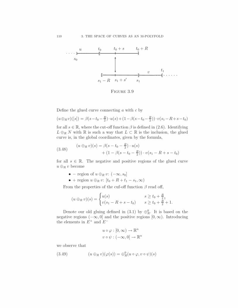
110 3. THE SPACE OF CURVES AS AN M-POLYFOLD
u
v t1
t0 + R
s1s1 + s′s1 − R
t0 + st0
s0
Figure 3.9
Define the glued curve connecting a with c by
(u⊕R v)([s]) = β(s−t0−R2) ·u(s)+(1−β(s−t0−
R2)) ·v(s1−R+s−t0)
for all s ∈ R, where the cut-off function β is defined in (2.6). IdentifyingL ⊕R N with R is such a way that L ⊂ R is the inclusion, the gluedcurve is, in the global coordinates, given by the formula,
(u ⊕R v)(s) = β(s − t0 −R2) · u(s)
+ (1 − β(s − t0 −R2)) · v(s1 − R + s − t0)
(3.48)
for all s ∈ R. The negative and positive regions of the glued curveu ⊕R v become
• − region of u ⊕R v: (−∞, s0]
• + region u ⊕R v: [t0 + R + t1 − s1,∞)
From the properties of the cuf-off function β read off,
(u ⊕R v)(s) =
{u(s) s ≥ t0 + R
2 1
v(s1 − R + s − t0) s ≥ t0 + R2
+ 1.
Denote our old gluing defined in (3.1) by ⊕0R. It is based on the
negative regions (−∞, 0] and the positive regions [0,∞). Introducingthe elements in E+ and E−
u ◦ ϕ : [0,∞) → Rn
v ◦ ψ : (−∞, 0] → Rn
we observe that
(3.49) (u ⊕R v)(ϕ(s)) = ⊕0R(u ◦ ϕ, v ◦ ψ)(s)

3.3. THE LEVEL-k CURVES AS AN M -POLYFOLD 111
a
b
c
a
b
c
uv
u v
t0
t0
t0 −R2
t0 + Rs1 − R
s1 −R2
s1
s1
t0 −R2
s1 −R2
⊕R(u, v)
Figure 3.10
as the following argument shows,
⊕0R(u ◦ ϕ, v ◦ ψ)(s)
= β(s − R2) · u ◦ ϕ(s) + (1 − β(s − R
2)) · v ◦ ψ(s − R)
= β(s − R2) · u(s + t0) + (1 − β(s − R
2)) · v(s + s1 − R)
= (u ⊕R v)(ϕ(s)).
Next we consider a level-3 curve.The negative and postive regions of u, v and w are characterized
by the pairs s0 ≤ t0, s1 ≤ t1 and s2 ≤ t2. Recall that the negativeand positive regions of the glued curve u ⊕R v connecting a with c ischaracterized by the pair s0 ≤ τ , where
(3.50) τ = t0 + R + t1 − s1.
Lemma 3.18. For gluing parameters R, R′ ≥ 2
(u ⊕R v) ⊕R′ w = u ⊕R (v ⊕R′ w).

112 3. THE SPACE OF CURVES AS AN M-POLYFOLD
u
v
w
a
bc
d
Figure 3.11
Proof. We first verify the associativity of the gluing by a compu-tation and give afterwards argument which such computations super-fluous. Recall that the cut-off function β satisfies β(s) = 0 for s ≥ 1and β(s) = 1 for s ≤ −1. Therefore, if R and R′ ≥ 2,
β(s − τ − R′
2) · β(s − t0 −
R2) = β(s − t0 −
R2)
and hence
(1 − β(s − t0 −R2)) · (1 − β(s − τ − R′
2)) = 1 − β(s − τ − R′
2),
where τ = t0 + R + t1 − s1. Using this we compute applying the gluingformula (3.48) twice, (
(u ⊕R v) ⊕R′ w)(s)
= β(s − τ − R′
2)(u ⊕R v)(s) + (1 − β(s − τ − R′
2)) · w(s + s2 − τ − R′)
= β(s − τ − R′
2) · β(s − t0 −
R2) · u(s)
+ β(s − τ − R′
2)) · (1 − β(s − t0 −
R2)) · v(s + s1 − t0 − R)
+ (1 − β(s − τ − R′
2)) · w(s + s2 − τ − R′)
= β(s − t0 −R2) · u(s) + (1 − β(s − t0 −
R2)) ·
[β(s − τ − R′
2) · v(s + s1 − t0 − R)
+(1 − β(s − τ − R′
2)) · w(s + s2 − τ − R′)
]= β(s − t0 −
R2)u(s) + (1 − β(s − t0 −
R2)) · (v ⊕R w)(s + s1 − t0 − R)
=(u ⊕R (v ⊕R′ w)
)(s).
�
Actually, the associativity of the gluing follows without any com-putations immediately from the following schematics procedure

3.3. THE LEVEL-k CURVES AS AN M -POLYFOLD 113
u
v
w
t0
s0
R
s1
t1 t1 + R′
s2 t2
R R′
u
v
w
a
b
c
d
Figure 3.12
Using our earlier notation and replacing the gluing parameter R byr related by the gluing profile
R = e1r − e
we shall in the following often write u ⊕r v instead of u ⊕R v andintroduce the notation
⊕(r1,r2)(u, v, w) = (u ⊕r1 v) ⊕r2 w = u ⊕r2 (v ⊕r2 w).
Consequently, for a level-k curve
([u1], . . . , [uk]) ∈ X(a0, a1) × · · · × X(ak−1, ak)

114 3. THE SPACE OF CURVES AS AN M-POLYFOLD
we define the successively by(3.51)⊕(r1,...,rk)(u1, . . . , uk) =
(. . .
(((u1 ⊕r1 u)2) ⊕r2 u3) ⊕r3 u4) . . .) ⊕rk
uk.
u1
u2
u3
u4
a1
a2a3
a4
Figure 3.13
In view of the above scheme the gluing is obviously associative andthe following general formula holds
⊕(r1,...,rk)(u1, . . . , uk)
=[⊕(r1,...,ri−1)(u1, . . . , ui)
]⊕ri
[⊕(ri+1,...,rk−1)(ui, . . . , uk)
].
In order to define the gluing of vector fields along curves we takeu ∈ X(a, b) and v ∈ X(b, c) whose ± regions are characterized by thepairs s0 ≤ t0 and s1 ≤ t1. Take a vector field h along u and a vectorfield k along v,
h(s) ∈ Tu(s)Rn − Rn
k(s′) ∈ Tv(s)Rn = Rn
for all s ∈ R and s′ ∈ R. In order to define the gluing and anti-gluingnear the corner b we take the coordinates ϕ and ψ in (3.47), so thatu ◦ ϕ : R+ → Rn and v ◦ ψ : R− → Rn, and consider the vector fields
h+(s) = h ◦ ϕ(s) ∈ Tu◦ϕ(s) = Rn
k−(s′) = k ◦ ψ(s′) ∈ Tv◦ψ(s′) = Rn
.
Denoting by ⊕0R(h+, k−) the old gluing formula from Section 3.3 we
define the gluing of vector fields h and k by
(h ⊕R k)(ϕ(s)) := ⊕0R(h ◦ ϕ, k ◦ ψ)(s)

3.3. THE LEVEL-k CURVES AS AN M -POLYFOLD 115
which leads to the formula
(h ⊕R k)(ϕ(s)) := β(s − t0 −R2) · h(s)
+ (1 − β(s − t0 −R2) · k(s1 − R + s − t0)
(3.52)
for all s ∈ R. The gluing intervals are chosen as in Figure 3.14
h
k
t0 t0 + R
s1 − R s1
Figure 3.14
From the properties of the cut-off function β one reads off,
(h ⊕R k)(ϕ(s)) :=
{h(s) s ≤ t0 + R
2− 1
k(s1 − R + s − t0) s ≥ t0 + R2
+ 1.
After the gluing, the information about h(s) for s ≥ t0 + R2− 1 and
k(s′) for s′ ≤ s1 −R2− 1 has disappeared. It will be recovered by the
anti-gluing formula for vector fields h and k, defined by
�R(h, k)(ϕ(s)) = ⊕0R(h ◦ ϕ, k ◦ ψ)(s)
for all s ∈ R, which leads to the formula
�R(h, k)(s) = −(1 − β(s − t0 −R2) · h(s)
+ β(s − t0 −R2) · k(s1 + R + s − t0)
(3.53)
for all s ∈ R. This time we have glued as in Figure 3.15.From (3.53) we read off
(h �R k)(ϕ(s)) :=
{k(s1 − R + s − t0) s ≤ t0 + R
2− 1
−h(s) s ≥ t0 + R2
+ 1.
Hence the anti-gluing contains the informations about the vectorfields outside of the gluing intervals towards the corner b. In coordinatesin which b = 0, the situation is illustrated by Figure 3.16.

116 3. THE SPACE OF CURVES AS AN M-POLYFOLD
−h
k
t0 t0 + R
s1 − R s1
Figure 3.15
uv
b = 0
−hk
t0
t0 + R2
s1 −R2
s1
Figure 3.16
Denoting by exp the exponential map associated with the Euclideanmatric on Rn we can define curves near u and b by
expu(h)(s) = expu(s)(h(s)) = u(s) + h(s)
expv(k)(s′) = expv(s′)(k(s′)) = v(s′) + k(s′)
for all s ∈ R and s′ ∈ R. From the gluing formul (3.48) fro curves and(3.53) for vector fields we read off the following results.
Lemma 3.19. If h and k are sections along the curves u ∈ X(a, b)
and v ∈ X(b, c), then
expu(h) ⊕R expv(k) = expu⊕Rv(h ⊕R k).
The effect of the anti-gluing is illustrated by the next statement.

3.3. THE LEVEL-k CURVES AS AN M -POLYFOLD 117
Proposition 3.20. Let (u, v) ∈ X(a, b) × X(b, c). If w ∈ X(a, c)is sufficiently close to u ⊕R v, then there exist unique vector fields halong u and k along v, so that
exp⊕r(u,v)(⊕r(h, k))(s) = w(s)
⊕r(h, k)(s) = 0
The two vector fields h and k are solutions of the two equations,
⊕R(u, v)(s) + ⊕R(h, k)(s) = w(s)
�R(h, k)(s) = 0
Consequently, by the gluing formulas (3.48), (3.52), and (3.53), abbre-viating τ(s) = β(s − t0 −
R2) and α = τ 2 + (1 − τ)2,[
τ 1 − ττ − 1 τ
]·
[h(s)
k(s1 − R + s − t0)
]=
[w(s) −⊕R(u, v)(s)
0
]The matrix is invertible. Hence[
h(s)k(s1 − R + s − t0)
]= R
α·
[τ τ − 1
1 − τ τ
]·
[w(s) −⊕R(u, v)(s)
0
],
so that the required solution is equal to
h(s) = τα· [w(s) −⊕R(u, v)(s)]
k(s1 − R + s − t0) = 1−τα
· [w(s) −⊕R(u, v)(s)].
Proof. We observe that the vector fields h along u and v along vsatisfy, in particular,
h(s) =
{w(s) −⊕R(u, v)(s) s ≤ t0 + R
2− 1
0 s ≥ t0 + R2
+ 1
k(s′) =
{0 s′ ≤ −R
2− 1
w(s′) −⊕R(u, v)(s′) s′ ≥ −R2
+ 1
Using the gluing construction one defines as in Section 3.1 a secondcountable topology on the set X which induces the original topologyon its corresponding parts.
In order to define a polyfold structure on the space X we look at asmooth representative
(u1, . . . , uk) ∈ X(a0, a1) × · · · × X(ak−1, ak)
of a level-k curve connecting a0 with ak. For every curve uj ∈ X(aj−1, aj)we fix a distinguished negative region (−∞, sj] and the positive region[tj,∞) so that uj(sj) is close to aj−1 and uj(tj) is close to aj . Since

118 3. THE SPACE OF CURVES AS AN M-POLYFOLD
aj−1 �= aj we find τj ∈ (sj , tj) such that the tangent vector uj(τj) doesnot vanish. Following the Recipe 1.37 we now find an sc-Banach spaceFuj
of vector fields along the smooth curve uj and an open neighbor-hood Ouj
⊂ Fujof the origin, such that the map
Auj:Ouj
→ X(aj−1, aj)
h �→ [expuj(h)]
defines a homeomorphism onto some open neighborhood Uj of [uj] inthe quotient space X(aj−1, aj). Next we shall define the sc-smoothsplicing projection πr on the sc-smooth Banach space
(3.54) E = Fu1 ⊕ Fu2 ⊕ · · · ⊕ Fuk
for the gluing parameter r = (r1, . . . , rk−1) ∈ [0, 1)k−1. For simplicitywe look at a level-3 curve again.
�
u
v
w
a
b c
d
Figure 3.17
Associated with u, v and w we have the positive regions defined bythe pairs s0 ≤ t0, s1 ≤ t1 and s2 ≤ t2. We first focus in a neighborhoodof the point b. If h is vector field along h and k a vector field along vwe consider, in coordinates ϕ and ψ from (3.47), the vector fields
h ◦ ϕ : [0,∞) → Rn
k ◦ ψ : (−∞, 0] → Rn.
In the notation of Section 2.2 we have h ◦ ϕ ∈ E+ and k ◦ ψ ∈ E−.We denote the old splicing from (2.8) by
π0r(h ◦ ϕ, k ◦ ψ) = (h ◦ ϕ, k ◦ ψ).

3.3. THE LEVEL-k CURVES AS AN M -POLYFOLD 119
Then the splicing for the two vector fields h and k along the curves
u and v are the two vector fields h and k along u and v defined by
(3.55) πr(h, k) = (h, k)
where (h, k) is given by
(h ◦ ϕ, k ◦ ψ) = π0r(h ◦ ϕ, k ◦ ψ).
Therefore, explicitly, with β denoting the cut-off function and α =β2 + (1 − β)2,
h(s) =β(s − t0 −
R2)
α(s − t0 −R2)·[β(s − t0 −
R2) · h(s)
+ (1 − β(s − t0 −R2)) · k(s − R + s1 − t2)
]k(′s) =
β(−s′ + s − R2)
α(−s′ + s − R2)·[(1 − β(−s′ + s − R
2)) · h(s′ + s1 −
R2)
+ β(−s′ + s − R2· k(s′)
]for all s, s′ ∈ R.
In view of the properties of the cuf-off function β we obtain, inparticular,
h(s) =
{h(s) s ≤ t0 + R
2− 1
0 s ≥ t0 + R2
+ 1
k(s′) =
{0 s′ ≤ s0 −
R2− 1
k(s′) s′ ≥ s1 −R2
+ 1
We see that outside of the gluing intervals the vector fields vanishtowards the corner b but remain unchanged towards the other side.
This defines h completely. For k, however, there is second conditioncomming from the other end of the curve v, namely, form the point c.Denoting by p a vector field along the curve w, we apply the definition(3.55) to the vector fields k and p along the curves v and w and obtain
(3.56) πr′(k, p) = (k, p),
where
k(s′) =β(s′ − t1 −
R′
2)
α(s′ − t1 −R′
2)·[β(s′ − t1 −
R′
2) · k(s′)
+ (1 − βs′ − t1 −R′
2) · p(s′ − R′ + s2 − t1)
].

120 3. THE SPACE OF CURVES AS AN M-POLYFOLD
In particular,
k(s′) =
{k(s′) s′ ≤ t1 + R′
2− 1
0 s′ ≥ t1 + R′
2+ 1.
Summarizing, the vector field k along the curve v connecting two pointswhere gluing takes place is determined by the two conditions πr(h, k) =
(h, k) and πr′(k, p) = (k, p), and satisfies, in particular,
k(s′) =
⎧⎪⎨⎪⎩0 s′ ≤ s1 −
R2− 1
k(s) s1 −R2
+ 1 ≤ s′ ≤ t1 + R′
2− 1
0 t1 + R′
2+ 1 ≤ s′.
The situation is illustrated by Figure 3.18.
a
b
c
d
t0
t0 + Rs1
s1 − Rt1 t1 + R′
s2 − R′
s2
Figure 3.18
Iterating this construction we obtain the sc-smooth projection mapπr : E → E satisfying πr ◦ πr = πr. One finds r0 ∈ (0, 1) such that forr = (r1, . . . , rk−1) ∈ [0, 1)k−1 the map
[0,∞)−k−1 ⊕ U1 ⊕ U1 ⊕ · · · ⊕ Uk → X
(r, h1, · · · , hk) �→ [⊕r(u1 + h1, . . . , uk + hk)]
if restricted to the splicing core, i.e., to the open set
O := ([o, r0)k−1 ⊕ U1 ⊕ · · · ⊕ Uk) ∩ KS ,
is a homeomorphism onto the open neighborhood U of ([u1], . . . , [uk]) inX. The inverse of the map defines a polyfold chart for X. The transi-tion maps between these charts are sc-smooth and we have constructeda polyfold structure for X.

3.3. THE LEVEL-k CURVES AS AN M -POLYFOLD 121
3.3.0.1. The Manifold Version. Assume that we are given a mani-fold M together with a countable collection of distinct points, say P ,so that every compact subset of M only contains finitely many. Forevery a ∈ P fix a sequence if weights δa
m starting at 0 and which isincreasing. We denote by X(a, b) the collection of equivalence classesof H2-curves R → M , connecting at −∞ the point a with the pointb at +∞. We define the level m to consist of equivalence class [u]represented by elements u which are in H2+m
loc and which are near −∞of class (m + 2, δa
m) and of class (m + 2, δbm) near +∞. For a finite
sequence a of mutually different points a = (a0, a1, .., ak) in P consider
X(a) = X(a0, a1) × .. × X(ak1 , ak).
We call k the length. Let P the collection of all such sequence of finitelength k ≥ 1. Define
X =∐a∈ bP
X(a).
If we consider a smooth level-k-map represented by (u1, ..., uk) we fixfor every ui a distinguished negative interval (−∞, ti] (if i > 0) anda distinguished positive interval [s,∞) (if i < k)). Let us denote thesequence of asymptotic limits by a0, ..., ak so that [ui] ∈ X(ai−1, ai).Fix a chart ϕi for i = 1, .., k − 1 around ai so that ϕi(ai) = 0. Weassume that the closures of their domains are disjoint and that theirimages contain the closed 2-balls around 0 ∈ Rn. We may assumethat the image of (−∞, si] under ϕi−1 ◦ ui−1 is contained in the 1
2-ball
and that the same holds for [ti,∞) under the map ϕi ◦ ui. Since theimage of the ui connects two different points we can find a numberτi ∈ (si, ti) where ui(τi) �= 0. Here we put s0 = −∞ and tk = +∞.We can pick charts around the ti mapping τi to 0 and having disjointdomains from the other charts so that the image again contains theclosed 2-ball around 0. Pull-back the standard Riemannian metric onthe 2-ball. Then we obtain a partially defined flat metric on M whichwe can extend smoothly. Following Recipe 1.37 we can define chartsaround the individual ui of the form
hi → [expui(hi)],
where hi(τi) ∈ Hi ⊂ Tui(τi)M is the constrained transversal to thederivative of ui at that point. Here hi lies in some Oui
. We assumethat all the properties hold as stated in Recipe 1.37.
Let us restrict for simplicity of notation to the case of a level-2-curve. The following procedure can be carried at every ai with 0 < i <k. Let u = ui, v = ui+1 and ψ = φi. The (nonlinear) gluing is defined
122 3. THE SPACE OF CURVES AS AN M-POLYFOLD
as follows:
ψ(⊕R(u′, v′)) = ⊕0R(ψ ◦ u′, ψ ◦ v′)
for u′ close to u and v′ close to v. Here ⊕0R denotes the Rn-gluing, i.e.
the model gluing. Since the exponential map comes from a metric flatnear a = ai the following holds. Take H2 sections h and k along u andv which are sufficiently small so that the following formula make sense.Denoting by dψ the map pr2 ◦ Tψ, i.e. the principal part we see
ψ(⊕R(expu(h), expv(k))
= ⊕R(ψ(expu(h)), ψ(expv(k)))
= ⊕0R(ψ(u), ψ(v)) + ⊕0
R(dψ(h), dψ(v)k)
= ψ(⊕R(u, v)) + ⊕0R(dψ(u)h, dψ(v)k)
= exp0ψ(⊕R(u,v))(⊕
0R(dψ(u)h, dψ(v)k))
= ψ(exp⊕R(u,v)(Tψ(⊕R(u, v)))−1(⊕0R(dψ(u)h, dψ(v)k))).
Let us define linear gluing as follows
⊕R(h, k) = Tψ(⊕R(u, v)))−1(⊕0R(dψ(u)h, dψ(v)k)).
Then ⊕R(h, k) is a section along ⊕R(u, v). Using these definitions wehave the following nice formula
Lemma 3.21. For h and k being sufficiently small sections along uand v we have
⊕r(expu(h), expv(k)) = exp⊕r(u,v)(⊕r(h, k)).(3.57)
Let us define next the anti-gluing �R(h, k). This will be a map
R → TaM
defined by
�R(h, k) := Tψ(a)−1(�0R(dψ(u)h, dψ(v)k)).
Lemma 3.22. Assume that u and v are as described above. Con-sider ⊕r(u, v) and assume that w is sufficiently close. Then there existsa unique pair of sections (h, k) of u∗TM and v∗TM so that
⊕r(h, k) = 0 and exp⊕r(u,v)(⊕r(h, k)) = 0.
Proof. This is a system of two equations. Using the definitions itis equivalent to
�0R(dψ(u)h, dψ(u)k) = 0
⊕0R(dψ(u)h, dψ(u)k) = ψ(w) − Ψ(⊕r(u, v))

3.3. THE LEVEL-k CURVES AS AN M -POLYFOLD 123
By the properties of the Rn-gluing and anti-gluing we see that dψ(u)hand dψ(v)k are uniquely determined. Hence the same is true for (h, k).
�
Next we have a look at the construction of charts. We have asuitable neighborhood Ou around zero in Fu and similarly Ov around0 ∈ Fv. The data is assumed to have the properties described by Recipe1.37. Then define for a sufficiently small r0 > 0
A : [0, r0) ⊕ Ou ⊕ Ov → X
by
A(r, h, k) = [⊕r(expu(h), expv(k))].
Observe that if A(r, h, k) = A(r′, h′, k′) then there exists t with
⊕r′(expu(h′), expv(k
′)) = t ∗ ⊕r(expu(h), expv(k)).
By the properties of the charts for X(a, b) and X(b, c) given by theRecipe, we see that t = 0 and R = R′ as before. If we know in additionthat �r(h, k) = �r(h
′, k′) it follows that the two pairs are equal. Letus define the associated splicing projection πr via the already studiedmodel splicing which we denote by π0
r . The obvious definition is givenby
πr(h, k) = (h, k),
with (h, k), (h, k) ∈ Fu ⊕ Fv, where (h, k) are defined by
(dψ(h)h, dψ(v)k) = πr(dψ(u)h, dψ(v)k).
From this we deduce that
h(s) =τ(s)2
α(s)h(s) +
τ(s)(1 − τ(s))
α(s)dψ(u(s)−1dψ(v(s − R))k(s − R).
There is a similar formula for k. It follows immediately from the defi-nition that πr is sc-smooth. In fact, the map
Fu ⊕ Fv → E : (h, k) → (dψ(u)h, dψ(v)k)
is a linear sc-isomorphism and therefore sc-smooth. Then π0r is a sc-
smooth splicing projection on E. Then this is followed by the inverseof the linear sc-operator. Hence (πr, Fu ⊕ Fv, [0, r0)) is a sc-smoothsplicing. Then the restriction to the splicing core gives a chart and allthese charts are smoothly compatible. Hence we have proved:

124 3. THE SPACE OF CURVES AS AN M-POLYFOLD
Theorem 3.23. The space of level-k-curves X in the manifold Mhas for given sequence δa = (δa
m) for every a ∈ P a natural M-polyfoldstructure where the charts have the form
(r1, .., rk−1, h1, .., hk) → [exp⊕(r1,..,rk−1)(u1,..,uk)(⊕(r1,..,rk−1)(h1, ..., hk))].

CHAPTER 4
M-Polyfold Bundles
4.1. Local Strong sc-Bundles
Prompted by constructions of pull back bundles later on we continuewith the conceptual framework and consider two Banach spaces E andF equipped with the sc-smooth structures defined by the filtrationsEm, resp. Fm for m ≥ 0. Their �-product
E � F
is the Banach space E ⊕ F equipped with the double filtration
(E � F )m,k = Em ⊕ Fk
where m ≥ 0 and 0 ≤ k ≤ m + 1.Similarly, if U ⊂ E is an open subset, then U � F is the open set
U ⊕ F equipped with the double filtration
(U � F )m,k = Um ⊕ Fk
for all m ≥ 0 and 0 ≤ k ≤ m + 1. Here Um = U ∩ Em, as introducedin Section 1.1. With the canonical projection map
U � F → U
we obtain a bundle, called a local strong sc-bundle . The �−tangentbundle of the product U � F is defined as
T(U � F ) = (TU) � (TF ).
Recalling the tangent bundle from Section 1.1, the �-tangent bundle isequipped with the double filtration,
T(U � F )m,k = (TU)m ⊕ (TF )k
= (Um+1 ⊕ Em) ⊕ (Fk+1 ⊕ Fk).
for all m ≥ 0 and 0 ≤ k ≤ m + 1.Recall the notation F0 = F . Associated with the product U �F one
has the derived sc-spaces
Un ⊕ F and Un ⊕ F 1
125

126 4. M-POLYFOLD BUNDLES
for every n ≥ 0. They are equipped with the standard (simple) filtra-tions
(Un ⊕ F )m = Un+m ⊕ Fm, m ≥ 0
(Un ⊕ F 1)m = Un+m ⊕ Fm+1, m ≥ 0.
Definition 4.1. If U �F → U and V �G → V are two local strongsc-bundles, then a sc0
�−map is a map
f : U � F → V � G
of the form
f(u, h) = (a(u), b(u, h))
which induces C0-maps
Um ⊕ Fk → Vm ⊕ Fk
for all m ≥ 0 and 0 ≤ k ≤ m + 1.
Recalling Definition 1.3 of a sc0-map we note that the map f ofclass sc0
induces sc0-maps between the derived sc-spaces
Un ⊕ F i → V n ⊕ Gi
for every n ≥ 0 and i = 0, 1. Recalling Definition 1.6 of an sc1-map weintroduce the next smoothness concept.
Definition 4.2. The sc0-map f : U � F → V � G is called of
class sc1
� if it induces sc1-maps between the derived spaces
Un ⊕ F i → V n ⊕ Gi
for every n ≥ 0 and i = 0, 1.
The tangent map associated with the sc1-map f is the sc0
-map
Tf : T(U � F ) → T(V � G)
defined by
(Tf)(u, h, v, k) = (a(u), Da(u)h, b(u, v), Db(u, v)[h, k])
where (u, h, v, k) ∈ Um+1 ⊕ Em ⊕ Fk+1 ⊕ Fk with 0 ≤ k ≤ m + 1.From the chain rule for sc1-maps (Theorem 1.13) one easily deducesthe following chain rule for sc1
-maps.
Theorem 4.3. Assume the maps f : U � F → R � G and g :V � G → W � H are of class sc1
, where U ⊂ E and V ⊂ R areopen subsets equipped with the induced sc-structures. Assume also that

4.2. STRONG SC-VECTOR BUNDLES 127
g(U �F ) ⊂ (V �G). Then the composition g ◦ f is also of class sc1 and
the tangent maps satisfy
T(g ◦ f) = (Tg) ◦ (Tf).
Moreover, T(g ◦ f) is sc0.
An sck�−vector bundle map is an sck
-map Φ : U � E → V � F ofthe form
Φ(x, h) = (a(x), b(x, h))
which is linear in h. The map Φ is called an sc-vector bundle isomor-phism, if it is sc-smooth and if the same also holds for the inversemap.
We distinguish between two different classes of sc-smooth sectionsof the local strong sc-bundle U � F → U .
Definition 4.4. An sc−smooth section f is a map of the form
u → (u, f(u)) ∈ U ⊕ F
so that the principal part f : U → F is sc-smooth. An sc-sectionf is called an sc+
− smooth section if its principal part induces ansc-smooth map f : U → F 1.
The tangent map Tf of a sc+-section f is a sc+-section of the �-tangent bundle TU � TF → TU . Let us denote the space of sc-smoothsections by Γ(U � F ) and that of sc+-sections by Γ+(U � F ). Assumethat Φ : U �F → V �G is an sc-vector bundle isomorphism. Then thepull back maps induce linear isomorphisms
Γ(V � G) → Γ(U � G)
and
Γ+(V � G) → Γ+(U � G).
The same, of course, holds true for the push-forward.
4.2. Strong sc-Vector Bundles
We use the discussion in Section 4.1 to define a useful class of sc-bundles over an sc-manifold. We consider two sc-manifolds X and Ysc-manifolds together with a surjective sc-smooth map
p : Y → X.

128 4. M-POLYFOLD BUNDLES
We assume that every fiber p−1(x) ⊂ Y has the structure of a Banachspace. To define an additional structure we now assume that we cancover Y with sc-charts. An sc� − chart is a tuple
(p−1(O), Φ, U � F )
where O ⊂ X is an open subset and
Φ : p−1(O) → U ⊕ F
is a homeomorphism which is fiber-wise linear and covers an sc-smoothchart
ϕ : O → U
so that pr1 ◦Φ = ϕ◦p. In addition, we assume that all transition mapsbetween our sc-charts
Ψ ◦ Φ−1 : ϕ(O ∩ O′) � F → ψ(O ∩ O′) � G
are sc-smooth vector bundle isomorphisms. Recall that this requiresthe following. The transition map Γ = Ψ◦Φ−1 necessarily has the form
Γ(u, h) = (ψ ◦ ϕ−1(u), b(u, h))
and is linear in h. In addition,
Γ : ϕ(O ∩ O′)n ⊕ F i → ψ(O ∩ O′)n ⊕ Gi
is sc-smooth for all the derived spaces with n ≥ 0 and i = 0, 1. Sum-marizing, we have constructed a strong sc-vector bundle structure forp : Y → X according to the following definition.
Definition 4.5. A strong sc-vector bundle structure for asurjective sc-smooth map p : Y → X between sc-manifolds consists ofthe following data. Every fiber has the structure of a Banach space.There is a maximal atlas of smoothly sc-compatible sc charts.
We point out that the postulated compatible sc-charts define adouble filtration Ym,k on Y where m ≥ 0 and 0 ≤ k ≤ m + 1. Themap p : Y → X maps Ym,k onto Xm. An element x ∈ X contained inXm is called of regularity m. The points y ∈ p−1(x) ⊂ Ym,k have fiberregularity k, where k is restricted to 0 ≤ k ≤ m + 1.
We remark that the tangent bundle p : TX → X1 is in general not!a strong sc-vector bundle for its natural structure (at least not in anatural way).
Clearly p is sc-smooth and surjective and the fibers have a Banachspace structure. The transition maps for sc-charts Tϕ and Tψ havethe form
T (ψ ◦ φ−1) : φ(O ∩ O′)1 ⊕ E → ψ(O ∩ O′)1 ⊕ F.

4.3. EXAMPLE OF A STRONG BUNDLE OVER X(a, b) 129
Let us write this for convenience shortly as
Γ : W 1 ⊕ E → V 1 ⊕ F.
It is straightforward to verify that the sc-smoothness implies that theinduced maps
Γ : W 1+n ⊕ E → V 1+n ⊕ F
are sc-smooth. In general the maps do not induce sc-smooth maps
Γ : W 1+n ⊕ E1 → V 1+n ⊕ F 1.
In fact this will, in general, not even be the case for n = 0. However, ifwe restrict the tangent bundle TX to X2, then TX|X2 → X2 admitsa natural sc-structure.
4.3. Example of a Strong Bundle over X(a, b)
Let X(a, b) be the sc-manifold consisting of the equivalence classesof maps R → M connecting the points a and b as introduced in Section1.5. We will construct a strong sc-vector bundle Y (a, b) over X(a, b).Choose [u] ∈ X(a, b). Then take a representative u and consider thepull back bundle u∗TM → R. If u is on level m, that is of classHm+2,δm, it makes sense to talk about Hm+2
loc -sections along u. Byusing trivialisations near a and b coming from charts we can definefor every ε ≥ 0 sections which in local coordinates near the ends haveweak derivatives up to order m which if weighted by eε|s| belong toL2. If 0 ≤ k ≤ m + 1, the space Hk+1,δk(u∗TM) is well-defined. Nowconsider pairs (u, h) of level (m, k) which by definition consist of a path
u ∈ X(a, b) of class m and h ∈ Hk+1,δk(u∗TM). Two such pairs areequivalent if they lie in the same orbit of the obvious R-action. Letus denote the whole collection by Y (a, b). Clearly we have a canonicalmap
Y (a, b) → X(a, b).
Also observe that at this point we have the double filtration Y (a, b)m,k →X(a, b)m with 0 ≤ k ≤ m + 1. Let us define next strong sc-vector bun-dle charts. They will be constructed out of our charts in the way aswe are familiar from the usual constructions of manifold of maps, see[12]. We give the inverses of the charts
(h, �) → [(expu(h),∇2 expu(h)�)].
Here h belongs to the usual neighborhoods of 0 ∈ Fu and � ∈ H1. Thetransition maps are clearly sc-smooth.

130 4. M-POLYFOLD BUNDLES
4.4. Strong M-Polyfold Bundles
4.4.1. Spliced Fibered Scales. Next we introduce a spliced ver-sion of our fibered scales. We take an open subset V of a partialcone and two sc-smooth Banach spaces E and H , and consider twosc-smooth splicings S0 = (π, E, V ) and S1 = (σ, H, V ) as defined inSection 2.1. The parameter set V is the same for both splicings.
In the following we denote by
[k, m]
a pair of integers satisfying 0 ≤ k ≤ m + 1.
Definition 4.6. A spliced sc-fibered Banach scale is the triplet
S = (Π, E � H, V )
where Πv = (πv, σv) : E � H → E � H is the family of projectionsparametrized by v ∈ V .
Taking two splicing cores K0 = KS0 = {(v, e) ∈ V ⊕ E| πv(e) = e}and K1 = KS1 = {(v, h) ∈ V ⊕ H| σv(h) = h} we can construct their�-product
KS� := K0 �V K1
having the double filtration defined by
(K0 �V K1)[k,m] = {(v, e, h) ∈ V ⊕ Em ⊕ Hk | πv(e) = e and σv(h) = h} .
The canonical projection
(V ⊕ E) � H → V ⊕ E
induces the natural sc-smooth projection
pr1 : KS� → KS0.
As before we can define a tangent splicing TS and the associatedsplicing core KTS� , so that T pr1 induces the projection
T pr1 : TKS� → TKS0 .
We are interested in pairs (KS�|O,S), where S is a spliced sc-fiberedBanach scale (Π, E � H, V ) and where
KS�|O
stands for the the preimage under the canonical projection
KS� → KS0

4.4. STRONG M-POLYFOLD BUNDLES 131
of an open subset O of KS0 ⊂ V ⊕ E. A smooth morphism
(KS�|O,S) → (KS′�|O′,S ′
)
is an sc-smooth map
KS�|O → KS′�|O′
of the form
(v, e, h) �→ (ϕ(v, πv(e)), Φ(v, πv(e), σv(h)))
where (v, e, h) ∈ O ⊕ H and ϕ(v, πv(e)) ∈ O′ ⊂ V ′ ⊕ E ′ and whereΦ(v, πv(e), σv(e)) ∈ H ′. Moreover, the fiber map Φ is linear in the
last argument. Recall from Section 2.3 that the subset O is open inV ⊕ E and defined by O = {(v, e) ∈ V ⊕ E | (v, πv(e)) ∈ O}. Simi-larly we can define the sc-sections and sc+-sections Γ(S, K
S�|O) andΓ+(S, K
S�|O). In future, if irrelevant, we might suppress the S inthe notation and simply write for example Γ(KS�|O). We also considersc-smooth vector bundle morphisms which are linear on the fibers.
4.4.2. M-Polyfold Bundles. Let Y and X be M-polyfolds andp : Y → X a surjective sc-smooth map so that the preimage of everypoint carries the structure of a Banach space.
Definition 4.7. A M-polybundle chart for p : Y → X is atriple (U, Φ, (KS�|O,S)), where U is an open set in X and Φ is ahomeomorphism
Φ : p−1(U) → KS�|O
which is linear on the fibers and is covering a homeomorphism
ϕ : U → O ⊂ KS0
so that pr1◦Φ = ϕ◦p. Moreover, Φ and ϕ are smoothly compatible withthe M-polyfold structures on Y and X. Two M-polybundle charts arecalled sc� − compatible provided the transition maps are sc-smoothlocal polyfold-bundle morphisms. A M-polybundle atlas consists ofa family of M-polybundle charts so that the underlying open sets Ucover X and so that the transition maps are sc-smooth. A maximalsmooth atlas of M-polybundle charts is called a M-polyfold bundlestructure.
The situation of an M-polyfold bundle chart is illustrated by thefollowing diagram.

132 4. M-POLYFOLD BUNDLES
Y ⊃ p−1(U)Φ
−−−→ KS�|O ⊂ KS�⏐⏐�p
⏐⏐�pr1
X ⊃ U −−−→ϕ
O ⊂ KS0
Here O is an open subset of the splicing core
KS0 = {(v, e) ∈ V ⊕ E | πe(v) = e},
where V is a partial cone in a finite dimensional vector space W andE is an sc-Banach space.
KS�|O = {(v, e, f) ∈ V ⊕ E ⊕ F | (v, e) ∈ O and σv(f) = f},
where F is an sc-Banach space. The fiber over (v, e) ∈ O is the Banachspace
pr−11 (v, e) = (v, e) × {f ∈ F | σv(f) = f}.
4.4.3. A Strong M-Polyfold Bundle over X. We have previ-ously introduced the strong sc-vector bundle Y (a, b) → X(a, b). Let usfirst study the case where the underlying manifold is Rn and considerthe M-polyfold of level-k-curves. We define Y → X in the obviousway and will show that it carries the structure of a strong M-polyfoldbundle.The local coordinates are constructed using a splicing core as-sociated to the strong local bundle
(Fu1 ⊕ .. ⊕ Fuk) � (H1(u∗
1TM) ⊕ .. ⊕ H1(u∗�TM) → Fu1 ⊕ .. ⊕ Fuk
with sc-structure given by quality ((m + 2, δm), (k + 1, δk)). In localcoordinates the splicing projections for fiber and basis are given bythe same formulas as before. If this splicing is denoted by S withunderlying splicing S0 we see that the inverse of charts have the form
(r1, .., rk−1, h1, .., hk, b1, .., bk) → [⊕r(∇2 expu1(h1)b1, ..,∇2 expuk
(hk)bk)],
where the data ranges in KS�|O and O is ithe mage of the chart in KS� ,and where ∇2 denotes the fiber derivative of the exponential map.

CHAPTER 5
Local sc-Fredholm Theory
We begin with a version of the implicit function theorem in our“sc-context”.
5.1. An Infinitesimal sc-Implicit Function Theorem
In order to study the local behavior of functions near a point wemake use of the concept of germs. If E is a Banach space with thesc-smooth structure
E = E0 ⊃ E1 ⊃ E2 ⊃ · · · ⊃ Em ⊃ · · ·
we denote by O(E, 0) an sc-germ of neighborhoods of 0 consisting of adecreasing sequence
U0 ⊃ U1 ⊃ U2 ⊃ · · · ⊃ Um ⊃ · · ·
where Um is an open neighborhood of 0 in Em for every m ≥ 0. Wepoint out that in contrast to the notation in Chapter 1, it is not requiredthat Um is induced from U0 as Um = U0 ∩ Em.
If F is a second Banach space with the sc-structure F = F0 ⊃ F1 ⊃F2 ⊃ · · · ⊃ Fm ⊃ · · · , then an sc0- germ
f : O(E, 0) → (F, 0)
is a continuous map f : U0 → F0 satisfying f(0) = 0 such that
f : Um → Fm
is continuous for every m ≥ 0. The sc-tangent germ O(E, 0) associ-ated with the neighborhoods Um belonging to O(E, 0) consists of thedecreasing sequence
Um+1 ⊕ Em, m ≥ 0
of open subsets of Em+1 ⊕ Em. An sc1- germ F : O(E, 0) → (F, 0) isan sc0-germ which, in addition, is of class sc1 in the sense of Definition1.6 or Proposition 1.7, however, this time with respect to the nestedsequence Um of the sc-neighborhood germ O(E, 0).
133
134 5. LOCAL SC-FREDHOLM THEORY
Definition 5.1. Consider a finite dimensional space V and an sc-Banach space E. Then an sc0-germ f : O(V ×E, 0) → (E, 0) is calledan sc0
− contraction germ if it has the form
f(v, u) = u − B(v, u)
so that the following holds. For every m ≥ 0 there is a constant 0 <ρm < 1 such that
‖B(v, u) − B(v, u′)‖m ≤ ρm · ‖u − u′‖m
for (v, u) and (v, u′) close to 0 in V × Em. Here the notion of closedepends on m.
We start with the following trivial consequence of a parameter de-pendent version of Banach’s fixed point theorem.
Theorem 5.2. Let f : O(V ⊕E, 0) → (E, 0) be an sc0-contractiongerm. Then there exists a uniquely determined sc0-germ δ : O(V, 0) →(E, 0) so that the associated graph germ gr(δ) : V → V ⊕ E, v �→(v, δ(v)) satisfies
f ◦ gr(δ) = 0.
Our main concern now is the regularity of the solution δ.
Theorem 5.3. If the sc0-contraction germ f : O(V ⊕E, 0) → (E, 0)is of class sc1, then the solution germ δ : O(V, 0) → (E, 0) in Theorem5.2 is also of class sc1.
Proof. We fix m ≥ 0 and show first that the set
(5.1)1
|b|‖δ(v + b) − δ(v)‖m
is bounded for v and b �= 0 belonging to a small ball around zero in Vwhose radius depends on m. Since the map B is of class sc1, there existsat (v, u) ∈ Um+1 a bounded linear map DB(u, v) ∈ L(V ⊕ Em, Fm),and we introduce the following notation,
DB(v, u)[v, u] = DB(v, u)[v, 0] + DB(v, u)[0, u]
= D1B(v, u)[v] + D2B(v, u)[u].
Since v �→ δ(v) is a continuous map into Em+1 and since the map B isof class C1 as a map from an open neighborhood of 0 in V ⊕Em+1 into

5.1. AN INFINITESIMAL SC-IMPLICIT FUNCTION THEOREM 135
Em, we have the identity
B(v + b, δ(v + b)) −B(v, δ(v + b)) =
[∫ 1
0
D1B(v + sb, δ(v + b))ds
][b].
As a consequence,
1
|b|‖B(v + b, δ(v + b)) − B(v, δ(v + b))‖m
≤
∫ 1
0
‖D1B(v + sb, δ(v + b))‖ds ≤ Cm.
(5.2)
Recalling δ(v) = B(v, δ(v)) and δ(v + b) = B(v + b, δ(v + b)) we havethe identity,
δ(v + b) − δ(v) − [B(v, δ(v + b)) − B(v, δ(v))]
= B(v + b, δ(v + b)) − B(v, δ(v + b)).(5.3)
From the contraction property of B in the second variable one concludes
(5.4) ‖B(v, δ(v + b)) − B(v, δ(v))‖m ≤ ρm‖δ(v + b) − δ(v)‖m.
Now, using 0 < ρm < 1 one derives from (5.3) using (5.2) and (5.4) theestimate
1|b|‖δ(v + b) − δ(v)‖m
≤1
1 − ρm·
1
|b|‖B(v + b, δ(v + b)) − B(v, δ(v + b))‖m
≤1
1 − ρm
· Cm
as claimed in (5.1). Since B is of class C1 from V ⊕Em+1 into Em andsince ‖δ(v + b) − δ(v)‖m ≤ C ′
m · |b| by (5.1), the estimate
(5.5) δ(v + b) − δ(v) − DB(v, δ(v)) · [b, δ(v + b) − δ(v)] = om(b)
holds true, where om(b) ∈ Em is a function satisfying 1|b|
om(b) → 0 in
Em as b → 0 in V . We next prove
(5.6) ‖D2B(v, δ(v))h‖m ≤ ρm · ‖h‖m
for all h ∈ Em+1. Fixing h ∈ Em+1, we can estimate

136 5. LOCAL SC-FREDHOLM THEORY
‖D2B(v, δ(v))h‖m
≤1
|t|· ‖B(v, δ(v) + th) − B(v, δ(v)) − D2B(v, δ(v))[th]‖m
+1
|t|· ‖B(v, δ(v) + th) − B(v, δ(v))‖m.
In view of the postulated contraction property of B, the second term isbounded by ρm · ‖h‖m, while the first term tends to 0 as t → 0 becauseB is of class C1. Hence the claim (5.6) follows. Using (5.6) and the factthat Em+1 is dense in Em, we derive for the continuous linear operatorD2B(v, δ(v)) : Em → Em the bound
(5.7) ‖D2B(v, δ(v))h‖m ≤ ρm · ‖h‖m
for all h ∈ Em. Thus, in view of ρm < 1, the continuous linear map
L(v) : Em → Em
L(v) := Id − D2B(v, δ(v))
is an isomorphism and we conclude from (5.5) the estimate in Em,
δ(v + b) − δ(v) − L(v)−1D1B(v, δ(v))b = om(b).
Therefore, the map v �→ δ(v) into Em is differentiable and its derivativeδ′(v) ∈ L(V, Em) is given by the formula
(5.8) δ′(v) = L(v)−1D1B(v, δ(v)).
It remains to show that v �→ δ′(v) ∈ L(V, Em) is continuous. Tosee this we define the map F : (V ⊕ V ) ⊕ Em → Em by setting
F (v, b, h) = D1B(v, δ(v))[b] + D2B(v, δ(v))[h].
The map F is continuous and, in view of (5.7), it is a contraction inh. Applying a parameter dependent version of Banach’s fixed pointtheorem to F we find a continuous function (v, b) �→ h(v, b) from asmall neighborhood of 0 in V ⊕ V into Em satisfying F (v, b, h(v, b)) =h(v, b). Since we also have F (v, b, δ′(v)b) = δ′(v)b, it follows from theuniqueness that h(v, b) = δ′(v)b and so the map (v, b) �→ δ′(v)b iscontinuous. Using now the fact that V is a finite dimensional space weconclude that v �→ δ′(v) ∈ L(V, Em) is a continuous map. The proof ofthe theorem is complete. �
Theorem 5.3 shows that the sc0-contraction germ f which is also ofclass sc1 has a solution germ δ satisfying f(v, δ(v)) = 0 which is also of

5.1. AN INFINITESIMAL SC-IMPLICIT FUNCTION THEOREM 137
class sc1. We shall show next, that if f is of class sc2, then δ is also ofclass sc2. To do so we define the sc0-germ f (1) by
f (1) : O(TV ⊕ TE, 0) → TE
f (1)(v, b, u, w) = (u − B(v, u), w − DB(v, δ(v))[b, w])
= (u, w) − B(1)(v, b, u, w),
where the last line defines the map B(1). For v small, the map B(1) hasthe contraction property with respect to (u, w). Indeed, on the m-levelof (TE)m = Em+1 ⊕ Em, i.e., for (u, w) ∈ Em+1 ⊕ Em and for (v, b)small we can estimate, using (5.6),
‖B(1)(v, b, u′, w′) − B(1)(v, b, u, w)‖m
= ‖B(v, u′) − B(v, u)‖m+1
+ ‖DB(v, δ(v))[b, w′] − DB(v, δ(v))[b, w]‖m
≤ ρm+1‖u′ − u‖m+1 + ‖D2B(v, δ(v))[w′ − w]‖m
≤ max{ρm+1, ρm} ·(‖u′ − u‖m+1 + ‖w′ − w‖m
)= max{ρm+1, ρm} · ‖(u
′, w′) − (u, w)‖m.
Consequently, the germ f (1) is an sc0-contraction germ. If now f is ofclass sc2, then the germ f (1) is of class sc1, as one verifies by comparingthe tangent map Tf with the map f (1) and using the fact that thesolution δ is of class sc1. Hence we deduce from Theorem 5.3 that thesolution germ δ(1) of f (1) is of class sc1. It solves the equation
(5.9) f (1)(v, b, δ(1)(v, b)) = 0.
But also the tangent germ Tδ defined by Tδ(v, b) = (δ(v), δ′(v)b) is asolution of (5.9). From the uniqueness we conclude δ(1) = Tδ so thatTδ is of class sc1, and hence δ of class sc2, as claimed. Proceedinginductively one verifes the following result.
Theorem 5.4. If f : O(V ⊕ E, 0) → (E, 0) is a contraction germwhich is, in addition, of class sck, then the solution germ
δ : O(V, 0) → (E, 0)
satisfyingf(v, δ(v)) = 0
is of class sck.
Proof. The proof is a consequence of the statements (k) belowwhich we prove by induction. In the following we denote by δj(v1) :V ⊕ · · · ⊕ V → E the j-th derivative of δ : V → E at the point v1. It

138 5. LOCAL SC-FREDHOLM THEORY
is a multilinear map (v2, · · · , vj+1) �→ δj(v1)[v2, · · · , vj+1]. Moreover,D1,jB(x1, · · · , xj) denotes the linearization of the function B with re-spect to the first variable x1 and the last variable xj . .
(k) Let f : O(V ⊕ E, 0) → (E, 0) be a contraction germ of class sck
and let δ : O(V, 0) → (E, 0) be a solution germ. Then δ is of class sck.Set B(1) = B and define f (1)(v1, h) = h−B(1)(v1, h) for (v1, h) ∈ V ⊕E.Then for every 2 ≤ j ≤ k there exists a map
(5.10) f (j) : V ⊕ V ⊕ · · · ⊕ V ⊕ E → E
of the form
(5.11) f (j)(v1, · · · , vj, h) = h − B(j)(v1, · · · , vj, h)
where
B(j)(v1, · · · , vj, h)
= D1,jB(j−1)
(v1, · · · , vj−1, δ
j−2(v1)[v2, · · · , vj−1])[vj , h]
(5.12)
having the following properties. If 1 ≤ j ≤ k, the germ (v1, · · · , vj) �→δj−1(v1)[v2, · · · , vj] solves the equation
(5.13) f (j)(v1, · · · , vj , δj−1(v1)[v2, · · · , vj ]) = 0.
Moreover, every map f (j) is multilinear with respect to (v2, v3, · · · , vj , h)and is a contraction germ with respect to h.
The statement (k) for k = 1 is just the conclusion of Theorem5.3. Now assume the statement to hold true for k ≥ 1. We shallprove that it holds true also for k + 1. Let f be of class sck+1. Byassumption (k), the solution germ v → δ(v) from V to E is of classsck. Since f is of class sck, the map B(k) is of class sc2 so that themap (v1, · · · , vk+1, h1, h) �→ D1,k+1B
(k)(v1, · · · , vk, h1)[vk+1, h], where(v1, · · · , vk+1, h1, h) ∈ V ⊕V · · ·V ⊕E1 ⊕E, is of class sc1. Composingthis map with the sc1-map
(v1, · · · , vk+1, h) �→ (v1, · · · , vk+1, δk−1(v1)[v2, · · · , vk], h)
we define the sc1-map
B(k+1)(v1, · · · , vk+1, h)
= D1,k+1B(k)(v1, · · · , vk, δ
k−1(v1)[v2, · · · , vk])[vk+1, h](5.14)
and introduce
(5.15) f (k+1)(v1, · · · , vk, h) := h − B(k+1)(v1, · · · , vk+1, h).

5.2. SC-FREDHOLM GERMS AND PERTURBATIONS 139
Abbreviating for the moment w = (v1, · · · , vk, δk−1(v1)[v2, · · · , vk])
and using the fact that B(k) is linear with respect to h we obtain forthe linearization in (5.14),
D1,k+1B(k)(w)[vk+1, h] = D1B
(k)(w)[vk+1] + D2B(k)(w)[h]
= D1B(k)(w)[vk+1] + B(k)(v1, · · · , vk, h).
This shows that f (k+1) is a contraction germ because, by assumption,B(k)(v1, · · · , vk, h) is a contraction with respect h. In addition, wesee that f (k+1) is linear with respect to the variables (v2, · · · , vk+1, h).Applying Theorem 5.3 to the map f (k+1), we find a unique map
(v1, v2, · · · , vk+1) → h(v1, · · · , vk+1)
from V ⊕ V ⊕ · · · ⊕ V to E which is of class sc1, solves the equation
h(v1, · · · , vk+1) = B(k+1)(w, h(v1, · · · , vk+1)),
and satisfies h(0, · · · , 0) = 0. On the other hand, by assumption (k),
δk−1(v1)[v2, · · · , vk] = B(k)(v1, · · · , vk, δk−1(v1)[v2, · · · , vk])
for (v1, v2, · · · vk) ∈ V ⊕ V ⊕ · · · ⊕ V . Differentiating this identity withrespect to v1 we find
δk(v1)[v2, · · · , vk+1] = D1B(k)(v1, · · · , vk, δ
k−1(v1)[v2, · · · , vk])[vk+1]
+ Dk+1B(k)(v1, · · · , vk, δ
k−1(v1)[v2, · · · , vk])[δk(v1)[v2, · · · , vk+1]]
= B(k+1)(v1, · · · , vk+1, δk(v1)[v2, · · · , vk+1]).
Hence, by uniqueness, δk(v1)[v2, · · · , vk+1] = h(v1, · · · , vk+1). Since(v1, · · · , vk+1) → h(v1, · · · , vk+1) is of class sc1, the map (v1, · · · , vk+1) →δk(v1)[v2, · · · , vk+1] is also of class sc1. This implies that the mapv �→ δ(v) is of class sck+1 as claimed. The proof of the theorem iscomplete.
�
5.2. sc-Fredholm Germs and Perturbations
After some preparation we shall introduce the crucial concept of agerm of an sc-Fredholm section.
5.2.1. Linearized sc-Fredholm Germs. Consider two sc-smoothBanach spaces E and F and a strong sc-bundle
b : U � F → U
where U is an open subset of E. If q is a smooth point, i.e., if
q ∈ U∞ = U ∩ U∞

140 5. LOCAL SC-FREDHOLM THEORY
then we denote by [b, q] or [U � F, q] the germ of b around the point q.Similarly, [f, q] denotes the germ of an sc- smooth section of the bundle[b, q] around the point q. If
b′ : U ′ � F ′ → U ′
is a second strong sc-bundle with the open set U ′ of E ′, we also choosea smooth point q′ ∈ U ′, take the germ [b′, q′] around the point q′ andconsider a germ of an sc-smooth section [g, q′] of the bundle [b′, q′].Assume that
[Φ, q] : [b, q] → [b′, q′]
is a germ of a strong sc-vector bundle isomorphism covering the germ[σ, q] of the sc-diffeomorphism satisfying σ(q) = q′. It is of the form
Φ(x, h) = (σ(x), ϕ(x)[h])
where our notation indicates that the fiber maps h → ϕ(x)[h] fromF to F ′ are linear sc-isomorphisms. Now define the germ [g, q′] of asmooth sc-section of [b′, q′] as the push-forward of the germ [f, q] ofsection of the bundle [b, q], as usual, by
g = Φ∗f := Φ ◦ f ◦ σ−1.
If f : U → F is the principal part of the section f and g : U ′ → F ′ theprincipal part of the section g, then
g(x) = pr2 ◦ Φ ◦ f ◦ σ−1(x) =: ϕ(x)[f ◦ σ−1(x)].
Linearizing g at the smooth point q′ = σ(q) we obtain by the chainrule the formula
Dg(q′)h = ϕ(q′)[Df(q) ◦ Dσ(q)−1h] + A(q′)[h],
where A(q′)[h] is the linearization of the map
(5.16) x → ϕ(x)[f(q)] ∈ (F ′)1
at the smooth point q′ in the direction h ∈ E1. Now, since Φ is a strongsc-vector bundle map, and since q and hence also f(q) are smoothpoints, the map (5.16) is an sc-smooth map U ′ → (F ′)1. Therefore,the linear map A(q′) : E ′ → F ′ is an sc+-map in the sense of Definition1.20. The linear map
h �→ ϕ(q′)[Df(q) ◦ Dσ(q)−1 · h]
from E ′ to F ′ is sc-Fredholm in the sense of Definition 1.18 if and onlyif Df(q) : E → F is an sc-Fredholm map. If this is the case, then weconclude from the stability of the Fredholm property in Proposition1.21 that the linear map Dg(q′) : E ′ → F ′ is also an sc-Fredholm map.
5.2. SC-FREDHOLM GERMS AND PERTURBATIONS 141
As a consequence we can define the following intrinsic property of thegerm [f, q].
Definition 5.5. If q is a smooth point, then an sc-smooth sectiongerm [f, q] of the strong sc-germ [b, q] is called linearized sc−Fredholm,if the linearization Df(q) of its principal part at q is sc-Fredholm inthe sense of Definition 1.18.
In view of the above discussion, the property of being linearized sc-Fredholm is invariant under (germs) of coordinate changes for strongsc-bundles. We summarize this fact as a proposition.
Proposition 5.6. If q is a smooth point, and if [f, q] is an sc-smooth germ of a section of a strong sc-vector bundle and [g, p] is thepush-forward by a strong sc-vector bundle isomorphism germ Φ, then[f, q] is linearized sc-Fredholm if and only if this holds true for [g, p].
From the stability of the Fredholm property under perturbations,formulated in Proposition 1.21, we deduce the following result.
Proposition 5.7. Let U be open in the sc-Banach space E andU � F → U be a strong sc-vector bundle. Assume that q ∈ U is smoothand [f, q] is a sc-smooth germ. Assume that [s, q] is a sc+-smooth germ.If [f, q] is linearized sc-Fredholm, then so is [f + s, q].
Proof. Taking the principal parts f and s we know that Ds(q) isan sc+-operator in the sense of Definition 1.20. Hence if Df(q) is ansc-Fredholm operator so is Df(q) + Ds(q) by Proposition 1.21 . �
5.2.2. sc-Fredholm Germs. Given the strong sc-smooth bundle
b : U � F → U,
where U ⊂ E is open, and given the smooth point q ∈ U , we considerthe germ [f, q] of an sc-smooth section around q.
Definition 5.8. The sc-smooth germ [f, q] of the strong sc-bundlegerm [b, q] is an sc−Fredholm germ, if the following two propertieshold true.

142 5. LOCAL SC-FREDHOLM THEORY
1) Regularizing property: for every m ≥ 0, there is a smooth openneighborhood Om ⊂ Um of q so that if p ∈ Om and f(p) ∈(U � F )m,m+1, then p ∈ Um+1.
2) Contraction property: there exists a partial cone V in Rn, ansc-smooth Banach space W , and a germ of a strong sc-vectorbundle isomorphism
Ψ : O(U � F, q) → O((V ⊕ W ) � (RN ⊕ W ), 0)
which covers the sc-diffeomorphism germ σ : O(U, q) → (V ⊕W, 0) satisfying σ(q) = 0 and which has the following property.If pr2 : (V ⊕W )�(RN ⊕W ) → RN ⊕W and P : RN ⊕W → Wdenote the canonical projections, then the sc-smooth germ
Ψ(f) : O(V ⊕ W, 0) → (W, 0)
Ψ(f)(v, w) := P ◦ pr2 ◦ [Ψ ◦ f ◦ σ−1(v, w) − Ψ(f(q))]
is an sc0-contraction germ in the sense of Definition 5.1.
Proposition 5.9. The sc-Fredholm germ [f, q] is a linearized sc-Fredholm section in the sense of Definition 5.5.
Proof. By assumption, the sc-smooth germ Ψ(f) is of the formΨ(f)(v, w) = w − B(v, w). Linearizing at the point (v, w) = 0 we find
DΨ(f)(0)[v, w] = w − D2B(0)w − D1B(0)v.
As in the proof of Theorem 5.3 one verifies that the linear opera-tor D2B(0) : Wm → Wm is a contraction for every m ≥ 0, i.e.,‖D2B(0)‖m < 1. Consequently,
Id − D2B(0) : W → W
is an sc-isomorphism. Since V is finite dimensional and since P projectsonto a subspace of finite codimension, it follows that the linearizationof the principal part of the push-forward of the section [f, q],
(v, w) → Ψ ◦ f ◦ σ−1(v, w),
at the point (0, 0) is an sc-Fredholm operator. From Proposition 5.6we conclude that [f, q] is a linearized sc-Fredholm section, as claimedin Proposition 5.9. �
Clearly, the property of being sc-Fredholm is also invariant undercoordinate changes of strong sc-bundles.
Proposition 5.10. Let f be an sc-smooth section of the bundleU � F → U . Assume that Φ : O(U � F, q) → O(U ′ � F ′, p) is a germof an sc-smooth vector bundle isomorphism. Then the section [f, q]
5.3. FILLERS AND LOCAL M-POLYFOLD FREDHOLM GERMS 143
is an sc-Fredholm germ if and only if the push-foward [Φ∗f, p] is ansc-Fredholm germ.
Finally, we are able to introduce sc-Fredholm sections.
Definition 5.11. An sc-smooth section f of the strong sc-vectorbundle U � F → F is called sc− Fredholm if at every smooth pointq ∈ U , the germ [f, q] is a an sc-Fredholm germ.
In view of the invariance under coordinate changes of strong sc-bundles, the definition immediately generalizes to strong sc-bundlesover sc-manifolds.
5.3. Fillers and Local M-Polyfold Fredholm Germs
Recalling the cumulating notations first we consider the two splic-ings S0 = (π, E, V ) and S1 = (σ, F, V ) having the same parameter setV which is an open subset of a partial cone in Rn. The spaces E andF are sc-smooth Banach spaces and
πv : E → E and σv : F → F
are the projections parametrized by v ∈ V as introduced in Section2.1. For fixed v we shall abbreviate the image of the projection πv inE by
K0,v = {e ∈ E| πv(e) = e}
and its complement in E by
Kc0,v = {e ∈ E| (Id−πv)(e) = e}
so that for every v ∈ V
(5.17) E = K0,v ⊕ Kc0,v.
Every e ∈ E splits accordingly to the splitting (5.17) into the sum
e = e1v ⊕ e2
v.
Similarly, the projection σv : F → F defines the splitting
(5.18) F = K1,v ⊕ Kc1,v.
Associated with the splicings S0 and S1 the spliced sc-fibered Ba-nach scale
S = ((π, σ), E � F, V )
has been introduced in Section 4.4. The �-product E �F is the Banachspace E⊕F equipped with the double filtration (E⊕F )m,k = Em⊕Fk

144 5. LOCAL SC-FREDHOLM THEORY
for m ≥ 0 and 0 ≤ k ≤ m + 1. The splicing cores associated with S0
and S1 are the image bundles of the projections,
K0 = KS0 = {(v, e) ∈ V ⊕ E| πv(e) = e}
K1 = KS1 = {(v, f) ∈ V ⊕ F | σv(f) = f}.
The total splicing core KS� is their �-product
KS� = K0 � K1
which as a set is equal to {(v, e, f) ∈ |(V ⊕E)�F | πv(e) = e and σv(f) =f}. The projection
(V ⊕ E) � F → V ⊕ E
induces the sc-smooth projection
KS� → KS0.
If O ⊂ KS0 be open subset of the splicing core, we shall study thebundle
(5.19) b : KS�|O → O
which is the local model for a strong M-polyfold bundle according toDefinition 4.7. A section
(5.20) f : O → KS�|O
is of the form(v, e1
v) �→ ((v, e1v), f(v, e1
v))
where f(v, e1v) ∈ K1,v ⊂ F . We use the same letter for the section
and the principal part of the section. According to Definition 2.8, thesection f is called sc-smooth if the extension
(5.21)f : O ⊂ V ⊕ E → F
f(v, e) := f(v, πv(e))
is sc-smooth on the open subset O of V ⊕ E defined by O = {(v, e) ∈V ⊕E| (v, πv(e)) ∈ O}. In the following we shall use the same letter falso for the extended function f . An sc-smooth section germ [f, q] ofthe bundle (b, q) consists of a smooth q ∈ O and an sc-smooth germ fof section of the bundle b : KS�|O → O.
Definition 5.12. A filler for the sc-smooth section germ [f, q]near a smooth point q ∈ V ⊕ E of the bundle (b, q) consists of an sc-
smooth section germ [f , q] of the bundle (V ⊕ E) � F → V ⊕ E whoseprincipal part has the form
(5.22) f(v, e) = f(v, e) + f c(v, e).

5.3. FILLERS AND LOCAL M-POLYFOLD FREDHOLM GERMS 145
Moreover, f c is defined on an open neighborhood of q in V ⊕E, mappingits points (v, e) into Kc
1,v in such a way that the mapping
(5.23)Kc
0,v → Kc1,v
e2v �→ f c(v, e1
v ⊕ e2v)
is a linear sc-isomorphism for every v and e1v, where e = e1
v ⊕ e2v is the
decomposition with respect to the splitting K0,v ⊕ Kc0,v = E.
By definition, f(v, e) ∈ K1,v and f c(v, e) ∈ Kc1,v. Hence one con-
cludes from
f(v, e) + f c(v, e) = 0
that f(v, e) = 0 and f c(v, e) = 0. Consequently, e2v = 0 so that e =
πv(e) = e1v and we see that the solution sets of the sections [f, q] and
[f , q] are naturally the same.
Definition 5.13. The sc-smooth germ [f, q] of a section of thelocal M-polyfold bundle (b, q) is called a polyfold Fredholm germ if
it possesses a filler f having the property that [f , p] is an sc-Fredholmgerm in the sense of Definition 5.8 at every smooth point p near q.
We point out that in dealing with germs around a smooth pointq we may always assume by means of a germ of an sc-diffeomorphismthat q = 0.
Setting q = 0 we consider the sc-smooth section germ f of the bun-dle (b, 0) defined in (5.19) and assume that its principal part satisfiesf(0) = 0. At v = 0 we have the sc-smooth Banach spaces
K0,0 = {e ∈ E| π0(e) = e}
K1,0 = {f ∈ F | σ0(f) = f}.
Recalling the splitting E = K0,0 ⊕ Kc0,0 and the corresponding de-
composition e = e10 + e2
0 we observe that f(0, e20) = 0 for all e2
0 ∈ Kc0,0.
Therefore, the linearization of f at the point 0 = (v, e) is the sc-linearmap
Df(0) : T0V ⊕ E → K1,0
(v, e) �→ Df(0)[v, e10],
where T0V = Rn. Now assume that the section f possesses the filler
f . Then the linearization of f at the point 0 is the sc-linear mapping

146 5. LOCAL SC-FREDHOLM THEORY
(5.24)Df(0) : T0V ⊕ E → F
Df(0)[v, e)] = Df(0)[v, e] + f c(0, e20)
where again e = e10 + e2
0 corresponds to the splitting E = K0,0 ⊕ Kc0,0.
Since f c(0, e20) ∈ Kc
1,0 we see that Df(0) is surjective if and only if the
linearized filler Df(0) is surjective. Because f c(0, e20) = 0 if and only if
e20 = 0, we conclude
ker Df(0) ⊂ T0V ⊕ K0,0
and
ker(Df(0)|T0V ⊕ K0,0) = kerDf(0).
5.4. Local solutions of polyfolds Fredholm germs
We shall demonstrate that the solution set of f = 0 of a polyfoldFredholm germ near a transversal smooth point carries in a natural waya smooth manifold structure. Using the infinitesimal implicit functiontheorem from Section 5.1, we shall reduce the problem by means of aLyapuonov-Schmidt type construction to a finite dimensional problem.We distinguish between the interior and boundary case.
5.4.1. Interior Case. We consider the polyfold Fredholm sectiongerm [f, 0] according to Definition 5.13. Its principal part
(5.25) f(v, e) = f(v, πv(e))
is sc-smooth in a neighborhood of 0 in V ⊕ E. We assume
f(0) = 0
and first study the special case in which the parameter set V of thesplicing is an open neighborhood of the origin in Rk. By the definition
of a polyfold Fredholm germ there exists a filler f of f which is asmooth section
f : O(V ⊕ E, 0) → O((V ⊕ E) � F, 0)
whose principal part is of the form
f(v, e) = f(v, e1v) + f c(v, e1
v + e2v),
the sum e1v + e2
v corresponding to the splitting E = K0,v ⊕ Kc0,v intro-
duced in (5.17). We shall assume now that the point 0 = (v, e) is atransversal point of the section f requiring the linearisation of f at 0,
Df(0) : T0V ⊕ E → F

5.4. LOCAL SOLUTIONS OF POLYFOLDS FREDHOLM GERMS 147
to be surjective. Note that T0V = Rk. Equivalently, the linearisation
of the filler f at 0,
Df(0) : T0V ⊕ E → F
is surjective. Since [f , 0] is, by assumption, an sc-Fredholm germ thereexists a germ of a strong sc-vector bundle diffeomorphism
Φ : O((V ⊕ E) � F, 0) → O((Rn ⊕ W ) � (RN ⊕ W ), 0)
so that the push forward section g = Φ∗f , if composed with theprojection pr2 onto its principal part and the natural projection P :RN ⊕ W → W , is a contraction germ according the Definition 5.1.Hence, for (a, u) ∈ Rn ⊕ W near the origin,
(5.26) P ◦ pr2 ◦ g(a, u) = u − B(a, u).
Explicitly, if
(5.27) Φ(v, e, h) = (σ(v, e), ϕ(v, e) · h)
with a diffeomorphism germ σ : O(V ⊕E, 0) → O(Rn⊕W, 0) satisfyingσ(0) = 0, the section has the principal part g : O(Rn ⊕ W, 0) →O(RN ⊕ W, 0) denoted by the same letter and defined by
g(a, u) = ϕ(σ−1(a, u)) · f(σ−1(a, u)).
It satisfies g(0) = 0. Abbreviating
ψ(a, u) = ϕ(σ−1(a, u))
τ(a, u) = σ−1(a, u),
the principal part becomes
(5.28) g(a, u) = ψ(a, u) · f(τ(a, u)).
Using f(0) = 0 the linerization of g at 0 = (a, u) is the sc-linearmapping
Dg(0)[b, h] = ψ(0) · Df(0) ◦ Dτ(0)[b, h]
for (b, h) ∈ Rn ⊕ W . By the assumption of transversality, the linear
operator Df(0) and hence also Df(0) is surjective. Since Dτ(0) andψ(0) are linear isomorphisms, the map
Dg(0) : Rn ⊕ W → RN ⊕ W
is also surjective. The solution set for g solves the equation
g(a, u) = 0
or, equivalently, the two equations

148 5. LOCAL SC-FREDHOLM THEORY
(5.29)Pg(a, u) = 0
(Id − P )g(a, u) = 0.
Since Pg(a, u) = u − B(a, u), the solutions of the first equation near0, are, in view of Theorem 5.3, represented as the graph of a functionδ : Rn → W so that
(5.30) Pg(a, δ(a)) = 0.
In fact these are all the solutions of the first equation locally near0 = (a, u). The function δ satisfies δ(0) = 0 and possesses, in viewof Theorem 5.4, the following regularity properties. Given any levelm and any integer j ≥ 0, there exists an open neighborhood O =O(m, j) ⊂ Rn of the origin so that if a ∈ O, then δ(a) ∈ Wm and themap δ : O → Wm is of class Cj . It remains to solve the second equationin (5.29) which becomes
(Id − P )g(a, δ(a)) = 0
and which is to be solved for a near the origin in Rn. We define themapping
G : Rn → RN
near 0 ∈ Rn by
(5.31) G(a) = (Id − P )g(a, δ(a)).
Given an integer j ≥ 1, there exists an open neighborhood O of theorigin in Rn on which G ∈ Cj(O, RN).
Lemma 5.14. The map DG(0) ∈ L(Rn, RN) is surjective.
Proof. The linearization of G at the point 0 is equal to
(5.32) DG(0)[b] = (Id − P )Dg(0) · [b, δ′(0)b]
for b ∈ Rn. Given (r, 0) ∈ RN ⊕ W we can solve the equation
(r, 0) = Dg(0)[b, h]
for (b, h) ∈ Rn ⊕W , in view of the surjectivity of Dg(0). Equivalently,there exists (b, h) ∈ Rn ⊕ W solving the two equations
r = (Id − P )Dg(0)[b, h]
0 = PDg(0)[b, h].
Explicitly, the second equation is the following equation
(5.33) 0 = −D1B(0) · b + [Id − D2B(0)] · h

5.4. LOCAL SOLUTIONS OF POLYFOLDS FREDHOLM GERMS 149
Recalling the proof of Theorem 5.3, the operator Id−D2B(0) : W → Wis a linear isomorphism. Therefore, given b ∈ Rn the solution h of theequation (5.33) is uniquely determined. On the other hand, linearizingPg(a, δ(a)) = 0 at the point a = 0 leads to PDg(0)[b, δ′(0)b] = 0 forall b ∈ Rn. Hence, by uniqueness h = δ′(0)b, so that the linear mapDG(0) in (5.32) is indeed surjective. �
We denote the kernel of DG(0) by C and take its orthogonal com-plement C⊥ in Rn, so that
C ⊕ C⊥ = Rn.
Then G : C⊕C⊥ → RN becomes a function of two variables, G(c1, c2) =G(c1 + c2) for which D1G(0) = 0 while D2G(0) ∈ L(C⊥, RN) is anisomorphism. By the implicit function theorem there exists a uniquemap c : C �→ C⊥ solving
(5.34) G(r + c(r)) = 0
for r near 0 and satisfying
c(0) = 0, Dc(0) = 0.
Moreover, given any j ≥ 1, there is an open neighborhood U of the ori-gin in C such that c ∈ Cj(U, C⊥). Summarizing we have demonstratedso far that all solutions (a, u) ∈ Rn ⊕ W of g(a, u) = 0 near the originare represented by
g(r + c(r), δ(r + c(r))) = 0
for r in an open neighborhood of 0 in C = kerDG(0) ⊂ Rn. Con-sequently, in view of formula (5.28), all solutions (v, e) ∈ V ⊕ E of
f(v, e) = 0 near the origin are represented by
f(β(r)) = 0
where β : C → Rk ⊕ E is defined near 0 by
β(r) = τ(r + c(r), δ(r + c(r))).
The function β satisfies β(0) = 0 and, of course, for every level m andevery integer j ≥ 1, there exists an open neighborhood U of 0 ∈ C suchthat if r ∈ U , then β(r) ∈ Rk ⊕Em and β ∈ Cj(U, Rk ⊕Em). From thedefinition of the filler it follows that β(r) ∈ K0. From the regularizingproperty in Definition 5.8 of an sc-Fredhom germ we conclude β(r) ∈Rk ⊕ E∞ so that
β(r) ∈ (Rk ⊕ E∞) ∩ K0.

150 5. LOCAL SC-FREDHOLM THEORY
Since the solution set of the filler f and of f are the same, all thesolutions (v, e) of f(v, e) = 0 near the origin are also represented by
f(β(r)) = 0
for r near 0 in C. In order to represent the solution set as a graph overthe kernel of the linearized equation at 0 we introduce
N : = kerDf(0)
= kerDf(0)|T0V ⊕ K0,0.(5.35)
In view of Proposition 5.9, the linear operator Df(0) ∈ L(Rk ⊕E, RN ⊕W ) is an sc-Fredholm operator in the sense of Definition 1.18.Hence dim N < ∞ and N ⊂ Rk ⊕ E∞ and we have an sc-splitting
N ⊕ N c = Rk ⊕ E.
By construction, the image of the linearization Dβ(0) ∈ L(C, Rk⊕E) is
equal to the kernel of Df(0). Moreover, from Dβ(0)·r = dτ(0)[r, δ′(0)r]it follows that Dβ(0) is also injective, so that Dβ(0) : C → N is a linearisomorphism. We define the map α : N → Rk ⊕ E near 0 ∈ N by
α(n) = β(Dβ(0)−1 · n).
The solution set is now parametrized by f(α(n)) = 0 for n near 0 ∈ N .Let Q : N ⊕ N c → N be the natural projection and consider themap Q ◦ α : N → N near 0. Since D(Q ◦ α)(0) = Id, it is a localdiffeomorphism leaving the origin fixed. We denote by γ the inverseof this local diffeomorphism satisfying Q ◦ α(γ(n)) = n for all small n.Then
α(γ(n)) = Q ◦ α(γ(n)) + (Id − Q)α(γ(n))
= n + (Id − Q)α(γ(n)).
The map
A : N → N c
near the origin in N is defined by A(n) = (Id −Q)α(γ(n)). It satisfiesA(0) = 0 and DA(0) = 0 and α(γ(n)) = n + A(n) so that
f(n + A(n)) = 0.
In addition, given any level m and any integer j there exists an openneighborhood U of 0 in N such that if n ∈ U , then A(n) ∈ N c
m and A ∈Cj(U, N c
m). We have demonstrated that the solution set of f(v, e) = 0near the transversal point 0 is represented as a graph over the kernelof the linearized map Df(0) of a function which is smooth at the point0.

5.4. LOCAL SOLUTIONS OF POLYFOLDS FREDHOLM GERMS 151
Proposition 5.15. Let V ⊂ Rk be an open neighborhood of theorigin and let [f, 0] be a polyfold Fredholm section germ according toDefinition 5.13 satisfying f(0) = 0. Let N be the kernel of Df(0)|T0V ⊕K0,0. Then dim N < ∞ and N ⊂ Rk ⊕ E∞ and there is an sc-complement N c so that
N ⊕ N c = Rk ⊕ E.
If Df(0) is surjective, then there exists a germ A : O(N, 0) → O(N c, 0)near 0 ∈ N satisfying A(0) = 0 and DA(0) = 0 such that for n near 0,
f(n + A(n)) = 0
n + A(n) ∈ (Rk ⊕ E∞) ∩ K0.
All solutions of f(v, e) = 0 in a sufficiently small neighborhood of theorigin in Rk ⊕ E are in the image of the map n �→ n + A(n). Inaddition. given any level m and any integer r j, there exists an openneighborhood U = U(m, j) ⊂ N of the origin on which A ∈ Cj(U, N c
m).
So far we have only used the fact that the filler f induces an sc-
Fredholm germ [f , 0] in the sense of Definition 5.8 at the point 0. We
next make use of the assumption that [f , q] is an sc-Fredholm germ atevery smooth point q in an open neighborhood of 0 in order to showthat the map n �→ n+A(n) is smooth on an open neighborhood of theorigin in N . We fix a level m and a sufficiently small neighborhoodO of the origin in N on which the map A : O → N c
m is of class C1.Choose a point n0 ∈ N near 0 and set
q0 = n0 + A(n0).
Then q0 is a smooth point and we shall apply Proposition 5.15 to thepoint q0 replacing the point q = 0 in there. This is possible in view ofthe next lemma.
Lemma 5.16. If n0 is small enough, the linearization Df(q0) :
Rk ⊕E → F is surjective and Fredholm. Moreover, dim [kerDf(q0)] =
dim [ker Df(0)] = dim N . Setting N ′ = kerDf(q0) the natural projec-tion p : N⊕N c = Rk⊕E → N induces an isomorphism p|N ′ : N ′ → N .
Proof. We use the notation in the proof of Proposition 5.15 andconsider equivalently the section g(a, u) defined in (5.28) and its lin-earization
(5.36) Dg(q0) : Rn ⊕ W → RN ⊕ W

152 5. LOCAL SC-FREDHOLM THEORY
at the point q0 = (a, δ(a)). In order to prove surjectivity we considerthe equation Dg(q0)[h, b] = [w, r] which in matrix notation accordingto the splitting in (5.36) becomes
(5.37)
[A A1
A2 A3
]·
[hb
]=
[wr
]with the linear operators
Ah = [Id − D2B(a, δ(a)] · h
A1b = D1B(a, δ(a)) · b
A2h = (Id − P )D2g(a, δ(a)) · h
A3b = (Id − P )D1g(a, δ(a)) · b
where (b, h) ∈ Rn ⊕ W and (r, w) ∈ RN ⊕ W . In view of the proof ofTheorem 5.3, the linear operator A : W → W is an sc-isomorphism.Hence the equation (5.37) for (h, b) becomes
(5.38)h = A−1w − A−1A1b
[A2A−1A1 − A3]b = A2A
−1w + r.
We abbreviate the continuous family of matrices
M(a) := [A2A−1A1 − A3] ∈ L(Rn, RN).
By assumption, Dg(0) is surjective. Therefore, if a = 0, then thematrix M(0) is surjective. Consequently, for small a the matrix M(a)is also surjective and so is the linear operator Dg(a, δ(a)). Choosingw = 0 and r = 0 in (5.38), the kernel of Dg(q0) is determined by thetwo equations
h = A−1A1b
[A2A−1A1 − A3]b = 0.
Consequently, the kernel is determined by the kernel of the matrixM(a). Setting K ′ = kerDg(q0) and K = kerDg(0) we conclude fromthe surjectivity of M(a) for small a that dimK ′ = dimK. In addi-tion, the natural projection p : K ⊕ Kc = Rk ⊕ E → K induces theisomorphism p|K ′ : K ′ → K and the lemma follows. �
Introducing
N ′ = kerDf(q0)
we have dimN ′ = dimN and Proposition 5.15 guarantees a map n′ �→n′ + A(n′) : N ′ → N ′ ⊕ (N ′)c defined for n′ near 0, satisfying A′(0) = 0and DA′(0) = 0, and solving
f(q0 + n′ + A′(n′)) = 0.

5.4. LOCAL SOLUTIONS OF POLYFOLDS FREDHOLM GERMS 153
Moreover, given integers m and j there is an open neighborhood U ofthe origin in N ′ on which A′ : U → (N ′)c
m is of class Cj. Denote by
p : N ⊕ N c → N
the natural sc-projection. Then p|N ′ : N ′ → N is an isomorphism if q0
is sufficiently close to 0, and we define the map α : N ′ → N near theorigin by
α(n′) = p[q0 + n′ + A′(n′)].
Then α(0) = n0 and, by the uniqueness of the solution set of f =0 near the origin, we have α(n′) + A(α(n′)) = q0 + n′ + A′(n′). Inaddition, Dα(0)h = p(h) for h ∈ N ′. Consequently, Dα(0) ∈ L(N ′, N)is an isomorphism and hence the map α is a local diffeomorphism. Inaddition, given any integer j there is an open neighborhood U of 0 ∈ N ′
on which α ∈ Cj(U, N). From the identity
n + A(n) = p[q0 + α−1(n) + A′(α−1(n))]
for n near n0 we conclude for given integers m and j that there is anopen neighborhood U(n0) of n0 ∈ N on which the map n �→ n + A(n)belongs to Cj(U(n0), Rk ⊕ Em). In particular, at the point n0, themap is smooth. The arguments apply to every n0 in a neighborhood ofthe origin in N . Therefore, we have demonstrated the following result,where in abuse of the notation we simply write
Df(0) = Df(0)|T0V ⊕ K0,0
and use the same letter f for the section and for its principal part.
Theorem 5.17. Let [f, 0] be a polyfold Fredholm germ as definedin Definition 5.13. Assume f(0) = 0 and denote by N the kernel of thelinearization Df(0). Then dim N < ∞ and N ⊂ Rk ⊕ E∞ and thereexists an sc-smooth complement N c so that
N ⊕ N c = Rk ⊕ E.
If Df(0) is surjective, there exists an open neighborhood O of the originin N and a smooth map A : O → N c satisfying A(0) = 0 and DA(0) =0 such that
f(n + A(n)) = 0
n + A(n) ∈ (Rk ⊕ E∞) ∩ K0
if n ∈ O. Moreover, A ∈ C∞(O, N cm) for every integer m. All solutions
of f(v, e) = 0 in a sufficiently small neighborhood of the origin in Rk⊕Eare in the image of the map n �→ n + A(n).

154 5. LOCAL SC-FREDHOLM THEORY
5.4.2. Boundary Case. So far, the parameter set V has been anopen neighborhood of the origin in Rn. In this subsection we considerthe case in which V is an open neighborhood of the origin in the partialcone
C = [0,∞)k × Rn−k
in Rn. There are many possible concepts for a submanifold in the pres-ence of boundaries or, more generally, of boundary with corners. Lateron we shall use a relatively strong concept called neat submanifolds.It has the advantage of a high degree of compatibility with the cornerstructure.
We consider the polyfold-Fredholm germ [f, 0] of the bundle O(K0�V
K1, 0) satisfying f(0) = 0, and abbreviate the linearization at 0 by
Df(0) = Df(0)|Rn ⊕ K0,0.
Note that Rn = T0V is the tangent space of the parameter set V at theorigin. The kernel
N = ker Df(0)
is a finite dimensional subspace of Rn ⊕ K0,0. We denote by
p : Rn ⊕ K0,0 → Rn
the canonical projection.
Definition 5.18. The polyfold-Fredholm germ [f, 0] is called neat,if the kernel N of the linearization Df(0) has the property
Rk × {0} ⊂ p(N).
We note that the subspace Rk ×{0} is the tangent space at 0 of thepart of V containing the corner.
Definition 5.19. If [f, 0] is neat and N the kernel of Df(0) inRn ⊕ K0,0, then an sc-complement R of N ,
Rn ⊕ K0,0 = N ⊕ R,
is called neat, ifR ⊂ ({0} × Rn−k) ⊕ K0,0.
Such a neat sc-complement does always exist. Indeed, take a k-dimensional subspace Z ⊂ N satisfying p(Z) = Rk × {0}. Then thesubspace Zc ⊂ N , determined by Zc = N ∩
(({0} × Rn−k) ⊕ K0,0
)has dimension dim N − k and satisfies Z ⊕ Zc = N . Let R be ansc-complement of Zc satisfying Zc ⊕ R = ({0} × Rn−k) ⊕ K0,0. ThenRn ⊕ K0,0 = N ⊕ R as claimed.

5.4. LOCAL SOLUTIONS OF POLYFOLDS FREDHOLM GERMS 155
Theorem 5.20. Let [f, 0] be a neat polyfold Fredholm section germof a strong local M-polyfold bundle satisfying f(0) = 0. If N is thekernel of the linearization Df(0) in Rn ⊕ K0,0, then dim N < ∞ andN ⊂ Rn ⊕ E∞ and there exists a neat sc-complement R such that
N ⊕ R = Rn ⊕ K0,0.
If Df(0) is surjective, then there exists an open neighborhood U of theorigin in N ∩ (C ⊕ K0,0) and an sc-smooth map
A : U → R
satisfying A(0) = 0 and DA(0) = 0 such that
f(n + A(n)) = 0
n + A(n) ∈ K0 ∩ (Rn ⊕ E∞)
for all n ∈ N . Moreover, A ∈ C∞(U, Rm) for every level m. Allsolutions of f(v, e) = 0 in a small neighborhood of the origin in C ⊕Eare in the image of the map n �→ n + A(n).
Proof. In view of the neatness requirement and recalling the lin-earization concept in the presence of corners from Remark ??, the prooffollows the lines of the proof of Theorem 5.17 with minor modifications.We keep the same notation as in the proof Theorem 5.17. Since thistime we are interested in parametrizing solutions (v, e) ∈ V ⊕ E off(v, e) = 0 where (v, e) is near the corner 0, we have to make sure thatthe maps defined in the proof of Theorem 5.17 are defined on openneighborhoods of 0 whose projections onto Rk are open neighborhoodsof 0 in [0,∞)k. Then the partial derivatives of these maps in the direc-tion of e1, · · · , ek of the standard basis for Rk are defined, and so thesemaps have well-defined linerizations at 0.
This time the diffeomorphism germ τ : O(Rn ⊕W, 0) → (V ⊕E, 0)which enters the definition of the sc-strong bundle diffeomorphism Φ(5.27) and the definition of the map g in (5.28), is a map
τ : [0,∞)l × Rm−l ⊕ W → [0,∞)k × Rn−k ⊕ E
satisfying τ(0) = 0. Since τ is a diffeomorphism, it follows that k = l.We abbreviate C = [0,∞)k × Rn−k and C0 = [0,∞)k × Rm−k. Settingτ = (τ1, τ2, τ3) where τ1, τ2, and τ3 take their values in [0,∞)k, Rn−k
and E respectively, the derivative of the map τ1 : [0,∞)k × Rm−k ⊕W satisfies D2τ1(0) = 0 and D3τ1(0) = 0. Moreover, the derivativeD1τ1(0) : Rk → Rk is an isomorphism. In addition, since τ1 ≥ 0, weconclude that D1τ1(0)[0,∞)k = [0,∞)k so that
Dτ(0)(C0 ⊕ W ) = C ⊕ E.
156 5. LOCAL SC-FREDHOLM THEORY
We are interested in solutions (a, u) of the equation g(a, u) = 0 for(a, u) ∈ C ⊕ W close to 0. As before g(a, u) = 0 is equivalent to thetwo equations
Pg(a, u) = 0
(1 − P )g(a, u) = 0
where P : RN ⊕ W → W is the canonical projection. In view ofTheorem 5.3, the solutions of the first equation are of the form (a, δ(a))with δ : C0 → W . The map δ has, by Theorem 5.4, the followingsmoothness property. For all integers m and j there is a neighborhoodO depending on j and the level m such that δ is of class Cj(O, Wm).
We introduce the map G : C0 = [0,∞)k × Rm−k → RN defined by
G(a) = (I − P )g(a, δ(a))
for a ∈ C0 and close to 0. As in the proof of Lemma 5.14 the linearmap DG(0) : Rk × Rm−k → RN is surjective. Its kernel K ⊂ Rm hasdimension equal to N − m and is isomorphic to the kernel N of the
linearization Df(0) : Rn⊕E → RN ⊕W . The isomorphism between Kand N is provided by the linear map h �→ Dτ(0)[h, δ′(0)h] for h ∈ K.The linear map
DG(0) : Rk × Rm−k → RN
is a surjection and so there are N columns j1 < j2 < . . . , jN of DG(0)which are linearly independent. The vectors D1τ1(0)e1, · · ·D1τ1(0)ek,where {e1, · · · , ek} is the standard basis of Rk span Rk, and we con-clude, in view of the neatness assumption, that j1 > k. Write theset {1, . . . , m} as the disjoint union of J = {j1, . . . , jN} and I ={i1, . . . im−N} with i1 < i2 < · · · < im−N . Since j1 > k, we havei1 = 1, i2 = 2, · · · , ik = k. Define RI = A1 × · · · × Am and RJ =B1 × · · ·Bm where Ai = R and Bi = {0} if i ∈ I and Ai = {0} and
Bi = R if i �∈ I. Consider the map G : (RI ∩ C0) × RJ → RN definedby
G(c1, c2) = G(c1 + c2).
The linearization of G at the point (c1, c2) = (0, 0) with respect to the
variable c2, D2G(0) : RJ → RN , is given by DG(0)h = DG(0)[0, h])for all h ∈ RJ , and so it is an isomorphism. Applying the implicitfunction theorem, we find open sets U0 ⊂ RI ∩ C0 containing 0 andV0 ⊂ RJ containing 0, and a map c : U0 → V0 such that c(0) = 0 and
G(r, c(r)) = G(r + c(r)) = 0. Hence all the solutions (v, e) ∈ C ⊕ E of
f(v, e) = 0 near the origin are of the form
β(r) = τ(r + c(r), δ(r + c(r))
5.4. LOCAL SOLUTIONS OF POLYFOLDS FREDHOLM GERMS 157
with r ∈ U0 ⊂ RI ∩ C. Since the zero set of the filler f coincides withthe zero set of f we see that
f(β(r)) = 0
for all r ∈ U . Now the linearization Dβ(0) : RI → C⊕E is clearly injec-
tive, and maps RI onto the kernel N of the linearization Df(0). HenceDβ(0) : RI → N is an isomorphism. In addition, if p : Rk×Rn−k⊕E →Rk is the canonical projection, then p(Dβ(0)C0) = [0,∞)k. Hence set-ting U1 = Dβ(0)U0 ⊂ N we see that p(U1) is an open neighborhood of0 in [0,∞)k. Then we introduce the map α : U1 → C ⊕ E by
α(n) = β(Dβ(0)−1n).
So that the zero set of f is parametrized by α(n) for n ∈ U1.In view of the neatness assumption there is a neat complementary
subspace R ∈ Rn⊕K0,0 so that N⊕R = Rn⊕K0,0. With the canonicalprojection Q : N ⊕ R → N we have Q ◦ α(n) = n for n ∈ U1 andD(Q ◦ α)(0) = Id. Hence there is an open neighborhood U of 0 inC ⊕K0,0 and map γ : U ∩N → U1 such that (Q ◦ α)(γ(n)) = n for alln ∈ U ∩ N . The map A : N → R takes the form
A(n) = (I − Q)(α ◦ γ)(n)
defined for n ∈ U ∩ N . The solution of f = 0 near the corner 0 are ofthe form n + A(n) so that
f(n + A(n)) = 0
for n ∈ U ∩ N . Clearly, A(0) = 0 and DA(0) = 0. Moreover, the mapA has the following smoothness property. For every integers j and mthere is an open neigborhood O (depending on j and m) of 0 in C⊕K0,0
such that A ∈ Cj(O∩N, Rm). In particular, A is smooth at the corner0. Summing up, we have shown that the solution set (v, e) ∈ C ⊕K0,0
of f = 0 near the corner 0 is represented as a graph of a map A definedon an open set in U2∩N and taking values in R. The set U2 is an openneighborhood of 0 in C ⊕ K0,0. Moreover, the map A is smooth at 0.
To finish the proof it remains to show that the map A is smooth atany other point of U ∩ N which is close to 0. Fix a level m. Withoutloss of generality we may assume that A is of class C1 on U2 ∩ N . Ifq ∈ C ⊕ E is close to the origin and f(q) = 0, then q = n + A(n)for the unique n ∈ U2 ∩ N . There is a ∈ C0 so that q = τ(a, δ(a)).Abbreviate by K(a) be the kernel of DG(a) and let N(a) be the kernel
of Df(q) where q = n + A(n) = τ(a, δ(a)). We already know that themap h �→ Dτ(a)[h, δ′(0)h] is an isomorphism between K(a) and N(a).We will show that if a ∈ C is close to 0, then N ⊕ R = N(a) ⊕ R and

158 5. LOCAL SC-FREDHOLM THEORY
Rk ×{0} ⊂ p(N(a)) where p : Rk ×Rn−k ⊕K0,0 → Rk ×Rn−k. Indeed,the columns j1 < · · · < jN with k < j1 of the matrix DG(0) arelinearly independent. So the matrix M(0) formed by these columnshas non zero determinant. In view of the continuity of DG(a) withrespect to a, the matrix M(a) formed by the same columns of thematrix DG(a) has non-zero determinant for a in C0 and close to 0.Hence the linearlization DG(a) : Rn → RN is surjective for a ∈ C andclose to 0. Moreover, if c1, . . . , cm−N is a basis for K = K(0), thenusing the implicit function theorem we find a basis c1(a), . . . , cn−N(a)for K(a) depending continuously on a and such that ci = ci(0) for1 ≤ i ≤ m − N . The corresponding basis n1(a), . . . , nm−N (a) for N(a)depends continuously on a. Arguing now as in the proof of Lemma1.22, we obtain that N ⊕R = N(a)⊕R for a ∈ C and close to 0. Fromthis and our neatness assumptions we deduce that Rk ×{0} ⊂ p(N(a))where p : Rn ⊕K0,0 → Rn is the canonical projection. In addition, thefact that N ⊕ R = N(a) ⊕ R implies that if p : N ⊕ R → N is thecanonical projection, then p|N(a) : N(a) → N is an isomorphism.
Fix a point n0 ∈ U2∩N and let q0 = n0 +A(n0). We will show thatA is smooth at n0. There is a point a0 ∈ C satisfying q0 = τ(a0, δ(a0)).We start with the case that some of the k first coordinates of p(q0)are equal to 0 where p : Rn ⊕ K0,0 = N ⊕ R → Rn is the canonicalprojection. Without loss of generality we may assume that the firstj coordinates of p(q0) are equal to 0. Then the first j coordinates ofp(n0) are also equal to 0 in view of the neatness assumption. Henceq∈[0,∞)j⊕Rn−j⊕E and q0 = τ(a0, δ(a0)). Since τ is a diffeomorphism,the first j coordinates of a0 are equal to 0 so that a0 ∈ [0,∞)j ×Rm−j.Abbreviate by K ′ = K(a0) the kernel of Dg(a0) and by the N ′ = N(a0)
the kernel of Df(q0) which is the same as the kernel of Df(q0)|Rn⊕K0,0.
The above discussion shows that Rk × {0} ⊂ p(N ′) and since j ≤ k,we see that the polyfold Fredholm germ [f, q0] is neat and there existsa complementary neat subspace R′ so that N ′ ⊕ R′ = Rn ⊕ K0,0.
Thus, we may apply the previous arguments and show the existenceof an open neighborhood U ′ of 0 in C⊕K0,0 and a map A′ : U ′∩N ′ → R′
such that all solution q of f(q) = 0 near q0 are of the form
q = q0 + n′ + A′(n′).
Moreover, the map A′ satisfies A′(0) = 0, DA′(0) = 0, and is smoothat the point n′ = 0.
Making U ′ smaller if necessary and recalling that the restriction ofthe projection p : N ⊕ R → N to N ′, p : N ′ → N , is an isomorphism,

5.4. LOCAL SOLUTIONS OF POLYFOLDS FREDHOLM GERMS 159
we define the map α : U ′ ∩ N ′ → U ∩ N by setting
α(n′) = p[q0 + n′ + A′(n′)].
We have α(0) = n0 and conclude that
(5.39) α(n′) + A(α(n′)) = q0 + n′ + A′(n′)
for all n′ ∈ U ′ ∩ N ′. The linearization Dα(0) : N ′ → N is well-definedand is an isomorphism. This implies that α is a local diffeomorphismbetween some open neighborhood of 0 in U ′∩N ′ and an open neighbor-hood of n0 in U ∩ N . We may assume that these open neighborhoodsare equal to U ′ ∩N ′ and U ∩N . The map α has the following smooth-ness property. For every integer j there exists an open neighborhoodO of 0 in U ′ ∩ N ′ is of class Cj on O. Since
n + A(n) = p[q0 + α−1(n) + A′(α−1(n))]
for n ∈ U ∩ N , we conclude that for given integers m and j thereexists an open neighborhood of O = Oj,m ⊂ U ∩ N of n0 such thatn �→ n + A(n) from O into Rn ⊕ (K0,0)m on which is of class Cj . Inparticular, the map n �→ A(n) for n ∈ U ∩ N and is smooth at 0 asclaimed.
Finally, if none of the the first coordinate of p(q0) is equal to 0, thenq0 is an interior point of C ⊕ E. Then q0 = τ(a0, δ(a0)) with a0 beingan interior point of C0. Moreover, if N ′ is the kernel of Df(q0), then,in view of Theorem 5.17, there is a map A′ : N ′ → R′ defined on anopen neighborhood of 0 in N ′ such the solutions of f = 0 near q0 areof the form n′ + A′(n′). Again we we have Rk × {0} ⊂ p(N ′) if q0 isclose to 0 and so the map α in (5.39) is well-defined. The rest of theproof is the same as above. The proof of the theorem is complete. �
5.4.3. Stability of local Fredholm sections. We shall demon-strate the useful fact that Fredholm sections are stable under appro-priate perturbations. As before we consider the local polyfold bundle
b : KS�|O → O
where O ⊂ K0 is open. The bundle
b1 : (KS�|O)1 → O
is defined over the level 1 open set O1 ⊂ O, and the set
KS� = {(v, e, f) ∈ (V ⊕ E) � F |πv(e) = e and σv(f) = f}
has the double filtration
(V ⊕ E)m+1 ⊕ Fk+1

160 5. LOCAL SC-FREDHOLM THEORY
for all m ≥ 0 and 0 ≤ k ≤ m+1. If q is a smooth point, then a section[f, q] of the bundle [b, q] induces a germ [f, q]1 of the bundle [b1, q]. FromDefinition 4.4 we recall that an sc1-section [s, q] of the bundle [b, q] hasthe property that the principal part is an sc-smooth map O → F 1.Hence, for all m ≥ 0 we have s(v, e) ∈ Fm+1 if (v, e) ∈ (V ⊕ E)m. Thestability result is now as follows.
Proposition 5.21. Suppose the section [f, q] is a polyfold Fredholmgerm of the bundle [b, q] in the sense of Definition 5.13. If [s, q] is ansc1-section of [b, q], then [f + s, q] is a polyfold Fredholm section germof the bundle [b1, q].
Proof. Denote by [f , q] the filler of [f, q] at the smooth point q.
We shall show that [f + s, q] is a filler for the germ [f + s, q] of the
bundle [b1, q]. We have to verify for f + s the two properties of an sc-
Fredholm germ in Definition 5.8. We first observe that f + s possessesthe regularizing property because the section s is sc+-smooth. In order
to verify the contraction property for f + s we use the fact that f is afiller. Hence there exists a partial cone V in Rn, an sc-smooth Banachspace W and a germ of a strong vector bundle isomorphism
Ψ : O(U � F, q) → O((V ⊕ W ) � (RN ⊕ W ), 0)
which covers the sc-diffeomorphism germ σ : O(U, q) → (V ⊕ W, 0)
satisfying σ(q) = 0 and which has the property that the map Ψ(f) :O(V ⊕ W, 0) → (W, 0) defined by
Ψ(f)(a, w) = P ◦ pr2 ◦ [Ψ ◦ f ◦ σ−1(a, w) − Ψ(f(q))],
is an sc0-contraction germ in the sense of Definition 5.1. Abbreviate
g(a, w) = Ψ(f)(a, w)
we have the contraction representation
g(a, w) = w − B(a, w).
Replacing f by the section s we define
S(a, w) = Ψ(s)(a, w).
Then S is an sc+-section. Abbreviating the linearization
Aw = D2S(0, 0)w,
w ∈ W , at the point (a, w) = (0, 0) in the direction of the secondargument. Then A : W → W is, on every level m ≥ 0, a compact

5.4. LOCAL SOLUTIONS OF POLYFOLDS FREDHOLM GERMS 161
operator. Therefore, Id+A : W → W is a linear sc-Fredholm operatorof index 0. The associated splitting of W ,
Id + A : W = C ⊕ X → W = R ⊕ Z
with C = ker (Id + A) and R = range (Id + A) satisfies dim C =dim Z < ∞. Since S is of class C1 on every level m ≥ 1 we have therepresentation
S(a, w) = Aw + G(a, w)
where D2G(0, 0) = 0. Hence G is a contraction with respect to thesecond variable on every level m ≥ 1 if only a and w are small enough(depending on the level m). Consider the sum
g(a, w) + S(a, w) = w − B(a, w) + Aw − G(a, w)
= (Id + A)w − B(a, w),
where
B(a, w) = B(a, w) + G(a, w).
The map B is a contraction in the second variable on every level m ≥ 1as long as a and w are sufficiently small. Define the canonical projec-tions
Q : W = C ⊕ X → X
E : W = R ⊕ Z → R,
and introduce
Φ(a, w) := E ◦ P ◦ pr2 ◦ [Ψ(f + s) ◦ σ−1(a, w) − Ψ((f + s)(q))]
= E ◦ [(id + A)w − B(a, w)]
= E ◦ (id + A) ◦ Q(Qw) − E ◦ B(a, (Id − Q)w + Qw).
Using the sc-isomorphism L := (Id + A)|X : X → R we obtain
L−1 ◦Φ(a, (Id −Q)w + Qw) = Qw + L−1 ◦E ◦ B(v, (Id−Q)w + Qw).
We shall view the set (a, (Id − Q)w) as the new parameter set anddefine
B((a, (Id − Q)w), Qw) := L−1 ◦ E ◦ B(a, (Id − Q)w + Qw).
Then B possesses the required contraction property with respect to thevariable Qw on all levels m ≥ 1 provided a and w are small enough. Itremains to identify the above expression as obtained from an admissible

162 5. LOCAL SC-FREDHOLM THEORY
coordinate change. For this we take any linear isomorphism τ : Z → Zand define the fiber transformation
Ψ = [(L−1 ◦ E) ⊕ τ ◦ (Id − E) ◦ Ψ.
With the projection
P : Rn ⊕ W = Rn ⊕ C ⊕ X → X
P (a, w) = Qw
we finally obtain, setting (a, (Id − Q)w + Qw) = (a, (Id − Q)w, Qw),the formula
P ◦ pr2 ◦ [Ψ ◦ (f + s) ◦ σ−1(a, (Id − Q)w, Qw) − Ψ ◦ (f + s)(σ−1(q))]
= Qw − B(a, (Id − Q)w, Qw).
We have proved that [f+s, q] is a polyfold Fredholm germ of the bundle[b1, q] in the sense of Definition 5.13. The proof of Proposition 5.21 iscomplete. �
CHAPTER 6
Global sc-Fredholm Theory
This chapter is devoted to the Fredholm theory in M-polyfold bun-dles.
6.1. Fredholm sections
Given the M-polyfold bundle
b : Y → X
according to Definition 4.7 we denote by Γ(b) the space of sc-smoothsections and by Γ+(b) the space of sc+-sections.
Definition 6.1. Fredholm section. A section f ∈ Γ(b) of theM-polyfold bundle b : Y → X is called Fredholm, if at every smoothpoint q ∈ X there exists an M-polyfold bundle chart
Φ : b−1(U) → KS�|O
around q ∈ U ⊂ X in the sense of Definition 4.7 in which the sectiongerm [f, q] is a local polyfold Fredholm germ according to Definition5.13. The collection of all Fredholm sections is denoted by F(b).
Recall that Definition 5.13 requires that [f, q] possesses a filler fwhich is an sc-Fredholm germ in the sense of Definition 5.8, and sopossesses the regularizing property and the contraction property.
From the local stability result in Proposition 5.21 one deduces im-mediately the following global version.
Proposition 6.2. The map
Γ(b) × Γ+(b) → Γ(b)
(f, s) �→ f + s
induces a mapF(b) × Γ+(b) → F(b1).
For the deeper study of Fredholm operators it is useful to introducefirst some auxiliary concepts.
163

164 6. GLOBAL SC-FREDHOLM THEORY
6.2. Mixed convergence and auxiliary norms
We begin with a notion of convergence in the bundle b : Y → Xcalled mixed convergence, referring to a mixture of strong convergencein the base space X and weak convergence in the level 1 fibers Y 1,assuming the fibers are reflexive sc-Banach spaces.
6.2.1. Mixed Convergence. We start with the local definitionin an M-polyfold bundle chart and consider the M-polyfold bundle
KS�|O → O
where O is an open subset of the splicing core
K0 := KS0 = {(v, e) ∈ V ⊕ E| πv(e) = e}
and where
KS� = {(v, e, y) ∈ O ⊕ F | σv(y) = y} = O � K1.
Abbreviating the elements in O by x = (v, e) we consider a sequence
(xk, yk) ∈ O � (K1)1,
where (K1)1 refers to F1, the level 1 space of the sc-Banach space F .
Definition 6.3. Mixed convergence. The sequence (xk, yk) ∈O � (K1)1 is called m-convergent to (x, y) ∈ O ⊕ F1 if
(1) xk → x in O
(2) yk ⇀ y in F1.
Symbolically,
(xk, yk)m−→ (x, y).
Lemma 6.4. If (xk, yk) ∈ O � (K1)1 and (xk, yk)m−→ (x, y), then
(x, y) ∈ O � (K1)1.
Proof. By assumption, xk = (vk, ek) and πvk(ek) = ek. Moreover,
σvk(yk) = yk. Since the inclusion map I : F1 → F0 is a compact map,
one concludes from the weak convergence of yk ⇀ y in F1 that yk → yin F0. With x = (v, e) it follows from the continuity of the projections(v, y) �→ σv(y) in F that σv(y) = y in F0. Since y ∈ F1 one concludesσv(y) = y in F1 so that (x, y) ∈ O � (K1)1 as claimed in the lemma.
�
We must demonstrate that the concept of m-convergence is compat-ible with M-polybundle maps provided the fibers are reflexive spacesaccording to the following definition.

6.2. MIXED CONVERGENCE AND AUXILIARY NORMS 165
Definition 6.5. An sc-Banach space F is called reflexive if allthe spaces Fm, m ≥ 0, of its filtration are reflexive Banach spaces.
We consider now an sc-smooth polybundle map
Ψ : O � K → O′ � K ′
assuming that the underlying sc-Banach spaces F and F ′ are reflexive.With x = (v, e) the map ψ is of the form
Ψ(x, y) = (σ(x), ψ(x, y)).
The maps σ : O → O′ and ψ are sc-smooth and linear in y. Considera sequence (xk, yk) ∈ O � (K1)1. If (xk, yk)
m−→ (x, y), then (x, y) ∈ O �
(K1)1 in view of Lemma 6.4, and σ(xk) → σ(x). From (xk, yk) → (x, y)in O � (K1)0 it follows that ψ(xk, yk) → ψ(x, y) in O′ � (K ′
1)0, so that
Ψ(xk, yk) → Ψ(x, y) in O′ � (K1)′0.
By Definition 4.2 of sc-smooth bundle maps, the map Ψ : O � (K1)1 →O′�(K ′
1)1 is continuous. From the continuity limk→∞ ψ(xk, y) = ψ(x, y)in (F ′)1 for all y ∈ F1, we deduce by means of the uniform boundednessprinciple that the sequence of bounded linear maps ψ(xk) ∈ L(F1, F
′1)
defined by ψ(xk) · y = ψ(xk, y) has uniformly bounded operator norms,|||ψ(xk)||| ≤ C for all k. Consequently, ‖ψ(xk, yk)‖1 ≤ C · ‖yk‖1. Fromthe weak convergence yk ⇀ y in F ′
1 we know that ‖yk‖1 is also abounded sequence. Hence ‖ψ(xk, yk)‖1 is a bounded sequence. Be-cause F ′
1 is a reflexive Banach space, every subsequence of the boundedsequence ψ(xk, yk) in F ′
1 possesses a subsequence having a weak limitin F ′
1. The limit is necessarily equal to ψ(x, y).Summarizing we have proved that
σ(xk) → σ(x) in O′
and
pr2 ◦ Ψ(xk, yk) ⇀ pr2 ◦ Ψ(x, y) in (K ′1)1
i.e., on level 1. The discussion shows that the mixed convergence is in-variant under M-polyfold chart transformations and hence an intrinsicconcept for M-polyfold bundles having reflexive fibers so that we canintroduce the following definition.
Definition 6.6. If b : Y → X is an M-polyfold bundle with reflex-ive fibers, then a sequence yk ∈ Y 1 is said to converge in the m-senseto y ∈ Y 1, symbolically
ykm−→ y in Y 1,

166 6. GLOBAL SC-FREDHOLM THEORY
if the underlying sequence xk = b(yk) ∈ X converges in X to an elementx and if there exists an M-polyfold bundle chart Ψ around the pointx ∈ X satisfying
pr2 ◦ Ψ(xk, yk) ⇀ pr2 ◦ Ψ(x, y)
weakly in (K ′1)1, i.e., on level 1.
As shown above, the definition does not depend on the choice ofthe local M-polyfold bundle chart.
6.2.2. Auxiliary Norms. For the general perturbation theory weintroduce some auxiliary concepts to estimate the size of perturbations.
Definition 6.7. An auxiliary norm N for the M-polyfold bundleb : Y → X consists of a continuous map N : Y 1 → [0,∞) having thefollowing properties.
• For every x ∈ X the induced map N |Y 1x → [0,∞) on the fiber
Y 1x = b−1(x) is a complete norm.
• For every m-convergent sequence ykm−→ y we have
N(y) ≤ liminfk→∞N(yk).
• If N(yk) is a bounded sequence and the underlying sequence xk
converges to x ∈ X then yk has a m-convergent subsequence.
In view of the open mapping theorem the complete norm N |Y 1 isequivalent to the original 1-norm. Using the paracompactness of X wecan easily construct auxiliary norms.
Proposition 6.8. Let b : Y → X be a M-polyfold bundle withreflexive fiber. Then there exists an auxiliary norm.
Proof. Construct for every x ∈ X via local coordinates a normNU(x) for Y 1|U(x) where U(x) is a small open neighborhood of x ∈ X.This is defined by NU(x)(y) =‖ pr2 ◦ Ψ(y) ‖1, where Ψ is a local m-polybundle chart and pr2 is the projection onto the fiber part. Observethat m-convergence of yk to some y in Y 1|U(x) implies weak conver-gence of pr2 ◦ Ψ(yk). Using the convexity of the norm and standardproperties of weak convergence we see that
NU(x)(y) ≤ liminfk→∞NU(x)(yk).
We have at this point local expressions for auxiliary norms which coverX. Using the paracompactness of X we can find a subordinate partition

6.2. MIXED CONVERGENCE AND AUXILIARY NORMS 167
of unity (χλ)λ∈Λ and define
N =∑
χλNU(xλ).
If N(yk) is bounded and the underlying sequence xk converges to somex ∈ X it follows in local coordinates that the representative of yk isbounded on level 1. In view of the reflexivity, the sequence yk possessesa m-convergent subsequence. �
The following result will be useful in compactness investigations.
Theorem 6.9 (Local Compactness). Consider the M-polyfold bun-dle b : Y → X having reflexive fibers and let f be a Fredholm sectionof b . Assume that an auxiliary norm N : Y 1 → [0,∞) is given. Thenthere exists at every smooth point q ∈ X an open neighborhood U(q) inX so that the following holds.
• The set Z defined by
Z = {x ∈ U(q)| f(x) ∈ Y 1 and N(f(x)) ≤ 1}
is a compact subset of X.• Every sequence (xk) in U(x) satisfying
lim infk→∞
N(f(xk)) ≤ 1
possesses a convergent subsequence.
Proof. The statement is local and, using in local coordinates thetranslation u �→ u− q which is sc-smooth since q is a smooth point, we
may assume that the filler f of the section f is defined near 0. Moreover,after a change of coordinates as in the definition of a contraction germ.we may assume that
f : V ⊕ W → RN ⊕ W
is defined near 0, where V ⊂ Rn is a partial cone. Denoting by P :RN ⊕ W → W the canonical projection, the contraction germ is givenby
P [f(a, w)− f(0)] = w − B(a, w).
It is defined on a sufficiently small closed neighborhood U0 of the originon the level 0 on which it has the contraction property. The auxiliarynorm N is defined on U 0⊕ (RN ⊕W )1 and, possibly choosing a smallerneighborhood, we may assume that it is equal to the 1-norm so thatN(x, h) = ‖h‖1. We now consider the set of (a, w) ∈ U 0 satisfyingf(a, w) ∈ (RN ⊕ W )1 and
‖f(a, w)‖1 ≤ 1.

168 6. GLOBAL SC-FREDHOLM THEORY
The section f splits according to the splitting of the tangent space into
f(a, w) =
[(Id−P )f(a, w)
Pf(a, w)
]=
[(Id−P )f(a, w)
w − B(a, w) + Pf(0)
].
Using the contraction property one finds for given u ∈ W close toPf(0) and given a ∈ V close to 0 a unique w(a, u) ∈ W solving theequation Pf(a, w(a, u)) = u. Moreover, the map (a, u) �→ w(a, u) iscontinuous on the 0-level. Now, given a sequence (ak, uk) ∈ U0 suchthat
f(ak, wk) =: (bk, uk)
belongs to (RN ⊕ W )1 and satisfies ‖f(ak, wk)‖1 ≤ 1, we have theequations
Pf(ak, wk) = uk
(Id−P )f(ak, wk) = bk
wk = w(ak, uk).
We shall show that (ak, wk) possesses a convergent subsequence in U 0.By assumption, (RN ⊕ W )1 is a reflexive Banach space so that goingover to a subsequence,
(bk, uk) ⇀ (b′, u′) in (RN ⊕ W )1
(bk, uk) → (b′, u′) in (RN ⊕ W )0,
and ‖(b′, u′)‖ ≤ 1. In RN we may assume ak → a′ ∈ V . Conse-quently, wk = w(ak, uk) → w′ := w(a′, u′). Hence f(a′, w′) = (b′, u′)and ‖f(a′, w′)‖1 ≤ 1. The proof of Theorem 6.9 is complete. �
6.3. Proper Fredholm Sections
In this section we introduce the important class of proper Fredholmsections.
Definition 6.10. A Fredholm section f of b : Y → X is calledproper provided f−1(0) is compact in X.
The first observation is the following.
Theorem 6.11 (∞-Properness). Assume that f is a proper Fred-holm section of the M-polyfold bundle b : Y → X. Then f−1(0) iscompact in X∞.
Proof. Properness implies by definition that f−1(0) is compacton level 0. Of course, f−1(0) is a subset of X∞ since f is regularizing.

6.3. PROPER FREDHOLM SECTIONS 169
Assume that xk is a sequence of solutions of f(x) = 0. We have toshow that it possesses a subsequence converging to some solution x0
in X∞. After taking a subsequence we may assume that xk → x0 onlevel 0. We choose a contraction germ representation for [f, x0]. Aftera suitable change of coordinates the sequence (ak, wk) corresponds toxk and the point (0, 0) to x0, and
wk = B(ak, wk),
with (ak, wk) → (0, 0) on level 0. Consequently,
wk = δ(ak)
for the map a → δ(a) constructed in Section 5.1 using Banach’s fixedpoint theorem on level 0. We know from Section 5.1 that for every levelm there is an open neighborhood Om of 0 so that δm : Om → W m iscontinuous and given by Banach’s fixed point theorem on the m-level.We may assume that Om+1 ⊂ Om. Fix a level m. For k large enough,we have ak ∈ Om. Then δm(ak) is the same as δ(ak) = wk. Henceak → 0 implies wk → 0 on level m. Consequently, (ak, wk) → 0 onevery level, implying convergence on the ∞-level. Hence xk → x0 inX∞ as claimed. �
As a consequence of the local Theorem 6.9 we obtain the followingresult for proper Fredholm sections.
Theorem 6.12. Let b : Y → X be an M-polyfold bundle with re-flexive fibers and assume that f is a proper Fredholm section. Assumethat N is a given auxiliary norm. Then there exists an open neigh-borhood U of the compact set S = f−1(0) so that the following holdstrue.
• For every section s ∈ Γ+(b) having its support in U and sat-isfying N(s(x)) ≤ 1, the section f + s is a proper Fredholmsection.
• Every sequence (xk) in U satisfying f(xk) ∈ Y 1 and
lim infk→∞
N(f(xk)) ≤ 1
possesses a convergent subsequence.
Proof. We know from the local Fredholm theory that f + s isFredholm if s is a sc+-section s. For every q ∈ S = f−1(0) there existsan open neighborhood U(q) having properties as in Theorem 6.9. SinceS is a compact set we find finitely many qi so that the open sets U(qi)cover S. We denote their union by U . Next assume that the support ofs ∈ Γ+(b) is contained in U . If f(x)+ s(x) = 0, then necessarily x ∈ U

170 6. GLOBAL SC-FREDHOLM THEORY
because otherwise s(x) = 0 implying f(x) = 0 and hence x ∈ S ⊂ U ,a contradiction. Consequently, the set of solutions of f(x) + s(x) = 0belongs to {x ∈ U | f(x) ∈ Y 1 and N(f(x)) ≤ 1} which by constructionis contained in a finite union of compact sets. The proof of Theorem6.12 is complete. �
6.4. Transversality and Solution Set
From our local considerations in the previous chapter we shall de-duce the main result about the solution set of Fredholm sections.
Theorem 6.13. Consider a proper Fredholm section f of the M-polyfold bundle b : Y → X. Assume that for every point q ∈ f−1(0) thelinearization Df(q) is neat and surjective. Then the solution set f−1(0)carries in a natural way the structure of a smooth compact manifoldwith boundary with corners.
Proof. Choose a point q ∈ X satisfying f(q) = 0. Then q is asmooth point, and there is a special M-polybundle chart (U0, Φ, KS�|O)as in Definition 4.7, where U0 is an open neighborhood around q in Xand Φ a homeomorphism
Φ : p−1(U0) → KS�|O
which is linear on the fibers and which covers a homeomorphism
ϕ : U0 → O ⊂ KS0 ,
so that pr1 ◦ Φ = ϕ ◦ b. Here O is an open subset of the splicing coreKS0 = {(v, e) ∈ V0 ⊕ E| πv(e) = e} where V0 = [0,∞)k × Rn−k is apartial cone, and E is an sc-Banach space. We may assume ϕ(q) = 0.Let g be the push-forward of the section f under Φ and let g be itsfiller. Then the linearization Dg(0) is by assumption surjective andneat. Denote by N the kernel of Dg(0). In view of Theorem 5.20,dim N < ∞ and N ⊂ Rn ⊕ E∞. Moreover, there exists a neat sc-complement R such that
N ⊕ R = Rn ⊕ K0,0.
In addition, there exists an open neighborhood V of zero in a partialcone of N and an sc-smooth map A : V → R satisfying A(0) = 0 andDA(0) = 0 such that the map
γ : V → N ⊕ R, γ(n) = n + A(n)
parametrizes all the solutions of g = 0 near the origin,
g(n + A(n)) = 0.

6.5. PERTURBATIONS 171
Further, n + A(n) ∈ N ⊕ R∞ ∩ K0. Composing the map γ with thecoordinate map ϕ we define the map β−1 : V → X by
β−1(n) = ϕ−1(n + A(n)) = ϕ−1 ◦ γ(n).
It parametrizes all solutions of f(x) = 0 near the point q. Denote byU ⊂ X the image of β−1, so that
U = β−1(V ).
The pair (U, β) will be a coordinate chart for the solution set f−1(0)and we shall show that all coordinate charts constructed this way aresmoothly compatible. Assume that (U ′, β ′) is a second such chart sothat U ∩ U ′ �= ∅ and consider
β ′ ◦ β−1 : β(U ∩ U ′) → β ′(U ∩ U ′).
By construction β ′ maps U ′ onto an open set V ′ of a partial cone inthe kernel N ′ which has neat sc-complement R′ and
(β ′)−1(n′) = (ϕ′)−1(n′ + A′(n′)).
Take p ∈ U ∩ U ′. Then β(p) = P ◦ ϕ(p) = P (n + A(n)) = n andβ ′(p) = P ′ ◦ϕ′(p) = P ′(n′ +A′(n′)) = n′ with the canonical projectionsP : N ⊕ R → N and P ′ : N ′ ⊕ R′ → N ′. Consequently,
n′ = β ′ ◦ β−1(n)
= P ′ ◦ ϕ′ ◦ β−1(n)
= P ′ ◦ ϕ′ ◦ ϕ−1(n + A(n))
= P ′ ◦ (ϕ′ ◦ ϕ−1) ◦ γ(n).
Since, by Theorem 5.20, the map γ is sc-smooth, and since the transi-tion map ϕ′ ◦ϕ−1 is, by definition, an sc-smooth map, the compositionβ ′ ◦ β−1 is sc-smooth and hence is a smooth map between open setsof partial cones in Euclidean spaces. The proof of Theorem 6.13 iscomplete. �
6.5. Perturbations
Let us next prove some perturbation results.
Theorem 6.14. Assume that f is a proper Fredholm section of theM-polyfold bundle b : Y → X. Let us assume that ∂X = ∅. Let N andα be auxiliary norm and bounds, respectively. Assume that U is theopen neighborhood of f−1(0) so that for every s ∈ Γ+(b) with supportin U and N(s(x)) ≤ α(x) the section f + s is proper. Denote thespace of all sections in Γ+ as just described by O. Then there exists for

172 6. GLOBAL SC-FREDHOLM THEORY
t ∈ 12O and ε ∈ (0, 1
2) a section s ∈ O with s − t ∈ εO so that f + s
has for every solution of f(q) + s(q) = 0 a surjective linearization.
Proof. The set Ξ of all x ∈ X with N(f(x)) ≤ α(x) and x ∈ U iscompact in X. Clearly Ξ ⊂ X1 by the regularizing property. Considerfor given t the solution set S of f + t = 0. This set is compact inX∞. For every x ∈ S consider the linearisation (f + t)′(x) which issc-Fredholm. We find finitely many sections s1, .., sk in Γ+(b) withsupport in U so that
(λ1, .., λk, h) → (f + t)′(x)h +
k∑i=1
λisi(x)
is onto. The same is true for all y close to x in X∞. By a finitecovering argument we can find finitely many section so that for every xwith (f + t)(x) = 0 the linearization (f + t)′(x) has a cokernel spannedby the s1(x), ..., sk(x). We may view Y as a M-polyfold bundle overRk ⊕ X. Then the map
(λ1, .., λk, x) → (f + t +k∑
i=1
λisi)(x)
gives a Fredholm section of Y 1 → Rk × X1 which has the propertythat along S the linearization is surjective. Let L be the solution setnear {0}×S. This is a smooth manifold and the projection L → Rk issmooth. Take a small regular value near 0. Then the associated sections∗ has the property that f + s∗ is transversal to the zero-section. �
6.6. An Example of a Fredholm Operator
We begin by proving some estimates which will be useful in showingthat the operator [u] → [du
dt+ f ′(u)] induces a Fredholm section of the
bundle p : Y → X.
6.6.1. An a priori estimate. We start by recalling the definitionof the Sobolev weighted spaces Hm,δ(S, Rn). If δ is a real number andI is an interval in R, then Hm,δ(I, Rn) consists of functions w whoseweak derivatives Djw up to order m belong to L2(I) if weighted byeδ|s|. The Hm,δ(I)-norm is defined by
‖w‖2Hm,δ(I) =
∑k≤m
∫I
|Dkw|2e2δ|s|ds.
In the following A : Rn → Rn is a symmetric linear isomorphismhaving the eigenvalues λi, 1 ≤ i ≤ n. As in Section 2.2 we work with
6.6. AN EXAMPLE OF A FREDHOLM OPERATOR 173
the sc-smooth Banach spaces E = E+ ⊕ E− consisting of pairs (u, v)of maps
(u, v) ∈ E+ ⊕ E− = H2([0,∞), Rn) ⊕ H2((−∞, 0], Rn).
The sc-structure is defined by the weighted Sobolev spaces E±m =
Hm+2,δm(R±) for all m ≥ 0, having the norms
‖w±‖2m =
∑j≤m+2
∫R±
|Djw±(s)|2e2δm|s|ds.
The norm on Em is defined as
‖(u, v)‖m = ‖u‖m + ‖v‖m.
Here δm, m ≥ 0 is a strictly increasing sequence starting at δ0 = 0but this time restricted by the condition
(6.1) δm < min{|λi|, 1 ≤ i ≤ n}.
Similarly, F = F+ ⊕ F− is the sc-smooth space consisting of pairs(h, k) of maps
(h, k) ∈ F+ ⊕ F− = H1(R+) ⊕ H1(R−)
with an sc-structure defined by the Sobolev spaces F±m = Hm+1,δm(R±).
We also recall from Section 2.2 the total gluing operation �r asso-ciating with (u, v) the pair of functions
(6.2) �r(u, v) = (⊕r(u, v),�r(u, v)).
If r > 0, it is explicitly given by
(6.3) �r(u, v) =
[τR(s) 1 − τR(s)
τR(s) − 1 τR(s)
]·
[u(s)
v(s − R)
]for 0 ≤ s ≤ R. Here τR(s) = β(s− R
2) with the cut-off function β from
(2.5) and
R = ϕ(r)
with the gluing profile ϕ from (2.6). We next introduce the 1-parameterfamily of sc-continuous linear operators
(6.4) Lr : E → F
defined, if r = 0, by
(6.5) L0(u, v) = (u + Au, v + Av)

174 6. GLOBAL SC-FREDHOLM THEORY
and if r ∈ (0, 1), by
(6.6) Lr(u, v) = �−1r
[(d
ds+ A
)(⊕r(u, v),�r(u, v)
)].
Explicitly, taking the derivative in s in the definition (6.2), a cal-culation shows that
(6.7) Lr(u, v) = L0(u, v) + FR(u, v)
where FR(u, v) = (F+R (u, v), F−
R (u, v)) is defined by the formulae
F+R (u, v)(s) =
τ (s)
α(s)· [(2τ(s) − 1) · u(s) − v(s − R)]
for all s ≥ 0, and
F−R (u, v)(s′) =
τ (−s′)
α(−s′)· [u(s′ + R) + (1 − 2τ(−s′)) · v(s′)]
for all s′ ≤ 0. We have abbreviated τ(s) = τR(s) and τ (s) = dds
τ(s).Moreover, α(s) = τ(s)2 + (1 − τ(s))2. Due to the definition of τ , thesupport of the function F+
R (u, v) is contained in the interval [R2−1, R
2+
1] ⊂ R+ while the support of F+R (u, v) is contained in [−R
2−1,−R
2+1] ⊂
R−. By Rellich’s compactness theorem, the linear operator FR : E → Fis compact. In view of Theorem 2.17, the maps (r, u, v) �→ F+
R (u, v)resp. (r, u, v) �→ F−
R (u, v) from [0, 12)⊕E → F+ resp. from [0, 1
2)⊕E →
F− are sc-smooth. We formulate this fact as a proposition.
Proposition 6.15. The map
L : [0, 1) ⊕ E → F
is sc-smooth.
We shall need in the following the well-known Fredholm propertiesof the linear operator L0 defined in (6.6).
Lemma 6.16. The operator L0 is sc-Fredholm with index 0 and withn-dimensional kernel and cokernel.
We denote by E the Sobolev space H2(R, Rn) of maps defined on
all of R. The sc-structure is given by the spaces Hm+2,δm(R). By Fwe denote the sc-smooth space Hm+1,δm(R) whose sc-structure is given
6.6. AN EXAMPLE OF A FREDHOLM OPERATOR 175
by the spaces Hm+1,δm(R). On these spaces we introduce the sc-linearcontinuous operator
L : E → F
Lw = w + Aw.
We will also need the sc-smooth space E = H2(R, Rn) with the sc-structure given by Em = Hm+2,−δm(R), and the space F = H1(R) withthe sc-structure defined by Fm = Hm+1,−δm(R). On these spaces wehave the sc-linear continuous operator L : E → F defined by Lw =w+Aw. In view of restriction (6.1) one verifies the following statement.
Lemma 6.17. The sc-linear operators L and L are sc-isomorphisms.
The above lemmata 6.16 and 6.17 are well-known and we refer, forexample to [19] and [26]. The aim of this subsection is the proof ofthe following a priori estimate.
Theorem 6.18. For every m ≥ 0 there exists a constant cm > 0 sothat
‖Lr(u, v)‖m + |u(0)| + |v(0)| ≥ cm · ‖(u, v)‖m
for all r ∈ [0, 12] and (u, v) ∈ Em.
Proof. Arguing indirectly we assume that on some level m thereare sequences rk → r0 and (uk, vk) ∈ Em satisfying ‖(uk, vk)‖m = 1and
(6.8) ‖(L0 + FRk)(uk, vk)‖m + |uk(0)| + |vk(0)| → 0
as k → ∞, where Rk = ϕ(rk).We consider two cases depending on whether the limit r0 is equal
to 0 or different from 0. We start with the case r0 > 0. In thiscase Rk → R0. The operator L0 is Fredholm with index 0 and FR0 is acompact operator, hence L0+FR0 is Fredholm with index 0. Denote byX the finite dimensional kernel of L0+FR0 and by Y the complementarysubspace in Em so that Em = X ⊕ Y . The restriction (L0 + FR0)|Y →Fm is injective. We split the sequence (uk, vk) accordingly into thesum (uk, vk) = (uk, vk) + (uk, vk) with (uk, vk) ∈ X and (uk, vk) ∈ Y .It follows from the definition of the operator FR that ‖FRk
(uk, vk) −FR0(uk, vk)‖m → 0 and since (L0 + FR0)(uk, vk) = 0 we conclude from(6.8) that
(6.9) ‖(L0 + FR0)(uk, vk)‖m → 0.

176 6. GLOBAL SC-FREDHOLM THEORY
The injectivity of (L0 + Fr0)|Y → Fm implies (uk, vk) → 0 in Em.Since the kernel X of L0 + Fr0 is finite dimensional and the sequence(uk, vk) bounded, we may assume without loss of generality that (uk, vk)converges in Em to (u, v) ∈ X. Consequently,
L0(u, v) + FR0(u, v) = 0.
This together with (u, v)(0) = 0 imply, in view of the uniqueness ofinitial value problem for differential equations, that (u, v) = 0. Hencewe have proved (uk, vk) → 0 in Em contradicting ‖(u, v)‖m = 1.
We next turn to the case r0 = 0. Again we shall reach a contra-diction by proving (uk, vk) → 0. We first show that we may assumeuk ≡ 0 and vk ≡ 0 on the intervals [0, 1] and [−1, 0] respectively. In-deed, the sequence uk considered over the interval [0, 2] is bounded inHm+2([0, 2]). Thus, in view of Rellich’s compact embedding theorem,we may assume without loss of generality that uk converges to u inHm+1([0, 2]). In particular, ‖uk − u‖H1([0,2]) → 0. From (6.8) we con-clude that ‖uk + Auk‖H0([0,2]) → 0 so that u + Au = 0 on [0, 2]. Thistogether with u(0) = 0 imply u = 0. Thus, ‖uk‖Hm+1([0,2]) → 0, hence
‖uk‖Hm+1([0,2]) ≤ ‖uk + Auk‖Hm+1([0,2]) + ‖Auk‖Hm+1([0,2]) → 0,
showing ‖uk‖Hm+2([0,2]) → 0. By the same argument, ‖vk‖H2+m([−2,0]) →0. Set λ(s) = β(s − 2) where β is the cut-off function introduced in(2.5). Then, ‖λuk‖Hm+2([0,2]) → 0 so that ‖(1−λ)uk, vk)‖m ≥ 3
4for large
k. Because the support of F+Rk
(uk, vk) is contained in [Rk
2−1, Rk
2+1]×
[−Rk
2− 1,−Rk
2+ 1] we have F+
Rk((1 − λ)uk, vk) = F+
Rk(uk, vk) so that
‖ dds
((1 − λ)uk)+A(1 − λ)uk + F+Rk
((1 − λ)uk, vk)‖m
= ‖(1 − λ)[uk + Auk + F+Rk
(uk, vk)] − λuk‖m
≤ C ·[‖L+
Rk(uk, vk)‖m + ‖λuk‖Hm+2([0,2])
]→ 0.
Similar reasoning applies for the sequence vk so that indeed we mayassume that (uk, vk) satisfies ‖(uk, vk)‖m ≥ 1
2and that the supports of
uk and vk are contained in [1,∞) and (−∞,−1].To proceed further we need some preparation. For the rest of the
proof we only consider pairs (u, v) ∈ E of functions for which thereexists s0 > 0 such that u(s) = 0 if s ∈ [0, s0] and v(s) = 0 if s ∈ [−s0, 0].Setting u(s) = 0 for s ≤ s0 and v(s) = 0 for s ≥ −s0 we consider thesefunctions as defined on all of R. Hence also the glued and anti-gluedfunctions are defined on all of R. We shall abbreviate them by
(6.10) (q, p) = (⊕r(u, v),�r(u, v))

6.6. AN EXAMPLE OF A FREDHOLM OPERATOR 177
and introduce the shifted functions
(6.11) (qR(s), pR(s)) = (q(s + R2), p(s + R
2))
defined for all s ∈ R. Equation (6.11) becomes
(6.12)
[qR
pR
]=
[β 1 − β
β − 1 β
]·
[u(s + R
2)
v(s − R2)
]where qR, pR and β are evaluated at s. For convenience we introducethe following abbreviations for the components of the map Lr : E → Fdefined in (6.7).
(6.13)L+
R(u, v) = u + Au + F+R (u, v)
L−R(u, v) = v + Au + F−
R (u, v).
By an easy calculations one verifies the formula
(6.14)
[qR + AqR
pR + ApR
]=
[β 1 − β
β − 1 β
]·
[L+
R(u, v)(s + R2)
L−R(u, v)(s − R
2)
]where qR, pR and β are evaluated at s. In the following we abbreviateδ = δm and write ‖w‖I for the L2-norm of a function w over the intervalI ⊂ R.
Lemma 6.19. There exists a constant Cm depending only on thecut-off function β such that
‖qR + AqR‖2Hm+2,−δ(R) ≤ Ce−δR
[‖L+
R(u, v)‖2m + ‖L−
R(u, v)‖2m
]‖pR + ApR‖
2Hm+2,δ(R) ≤ Ce−δR
[‖L+
R(u, v)‖2m + ‖L−
R(u, v)‖2m
].
Proof. We only consider the first estimate since the proof of thesecond is similar. To simplify the notation we drop the functions uand v together the index R in L+
R(u, v)(s) and L−R(u, v)(s), writing
L+(s) and L−(s) instead. Using (6.14) we have the following pointwiseinequality for 0 ≤ j ≤ m + 2,
|Dj(qR + AqR)|2
≤ C · [ |Dj(β · L+(s + R2))|2 + |Dj((1 − β) · L−(s − R
2))|2 ].
In view of the properties of β, and since L+(s + R2) = 0 if s ≤ −R
2
and L−(s− R2) = 0 if s ≥ R
2, the first summand on the right hand side
above is supported in the interval [−R2, 1] and the second in the interval

178 6. GLOBAL SC-FREDHOLM THEORY
[−1, R2]. After multiplying both sides above by e−2δ|s| and integrating
over R we find
‖[Dj(qR + AqR)]e−δ|s|‖2R
≤ C ·[‖[DjL+(s + R
2)]eδs‖2
[−R2
,0]+ ‖[DjL+(s + R
2)]e−δs‖2
[0,1]
+ ‖[DjL−(s − R2)]eδs‖2
[−1,0] + ‖[DjL−(s − R2)]e−δs‖2
[0, R2
]
].
We estimate each of the terms on the right hand side.
‖[DjL+(s + R2)]eδs‖[−R
2,0] = e−δ R
2 ‖[DjL+(s + R2)]eδ(s+ R
2)‖[−R
2,0]
≤ e−δ R2 ‖[DjL+(s)]eδs‖R+ ,
and
‖[DjL+(s + R2)]e−δs‖[0,1] = e−δ R
2 · ‖[DjL+(s + R2)]eδ(s+ R
2)e−2δs‖[0,1]
≤ e−δ R2 · ‖L+(s + R
2)eδ(s+ R
2)‖[0,1] ≤ e−δ R
2 · ‖L+(s)eδs‖R+ .
Similarly
‖[DjL−(s − R2)]eδs‖[−1,0] ≤ e−δ R
2 ‖[DjL−(s)]e−δs‖R−
‖[DjL−(s − R2)]e−δs‖[0, R
2] ≤ e−δ R
2 · ‖[DjL−(s)]e−δs‖R−.
Summing from j = 0 to j = m + 1 we obtain
‖qR + AqR‖2Hm+2,−δ(R) ≤ Ce−δR
[‖L+‖2
m + ‖L−‖2m
].
as claimed. The proof of the lemma is complete. �
Multiplying the matrix equation (6.12) by the inverse matrix oneobtains the formula
(6.15)
[u(s + R
2)
v(s − R2)
]=
1
α·
[β β − 1
1 − β β
]·
[qR
pR
]where β, qR and pR are evaluated at s and where α = β2 + (1 −
β)2. Proceeding as in the proof of Lemma 6.19, using (6.15) and theproperties of β as well as the facts that qR(s) = 0 for s ≤ −R
2and
pR(s) = 0 for s ≥ R2, one proves the following lemma.
Lemma 6.20. There exists a constant Cm > 0 depending only onthe cut-off function β such that
‖u‖2m ≤ CeδR
[‖qR‖
2Hm+2,−δ(R) + ‖pR‖
2Hm+2,δ(R)
]‖v‖2
m ≤ CeδR[‖qR‖
2Hm+2,−δ(R) + ‖pR‖
2Hm+2,δ(R)
].

6.6. AN EXAMPLE OF A FREDHOLM OPERATOR 179
Having Lemma 6.19 and Lemma 6.20 at hand we can finish theproof of Theorem 6.18. We set
qRk(s) = ⊕Rk
(uk, vk)(s + Rk
2) and pRk
(s) = �Rk(uk, vk)(s + Rk
2).
Recalling the operators L : Em → Fm and L : Em → Fm from Lemma6.17, we conclude from Lemma 6.19
‖L(eδRk2 qRk
)‖Hm+2,−δ(R) → 0 and ‖L(eδRk2 pRk
)‖Hm+2,δ(R) → 0.
as k → ∞. The operators L and L are isomorphisms, hence
‖eδRk2 qRk
‖Hm+2,−δ(R) → 0 and ‖eδRk2 pRk
‖Hm+2,δ(R) → 0.
Applying Lemma 6.20,
‖uk‖m → 0 and ‖vk‖m → 0.
Recalling δ = δm this means that (uk, vk) → 0 in Em in contradictionto ‖(uk, vk)‖m ≥ 1
2. This finishes the proof of Theorem 6.18.
�


Bibliography
[1] V. Borisovich, V. Zvyagin and V. Sapronov, Nonlinear Fredholm maps andLeray-Schauder degree, Russian Math. Survey’s 32:4 (1977), p 1-54.
[2] R. Bott and L. W. Tu, Differential forms in algebraic topology, Springer, NewYork, 1982.
[3] F. Bourgeois, Y. Eliashberg, H. Hofer, K. Wysocki and E. Zehnder, Compact-ness Results in Symplectic Field Theory, Geometry and Topology, Vol. 7, 2003,pp.799-888.
[4] W. Chen and Y. Ruan, Orbifold Gromov-Witten theory, preprint.[5] K. Cieliebak, I. Mundet i Riera and D. A. Salamon, Equivariant moduli prob-
lems, branched manifolds, and the Euler class, Topology 42 (2003), no. 3,641–700.
[6] J. Dungundji, Topology, Allyn and Bacon, 1966.[7] Y. Eliashberg, A. Givental and H. Hofer, Introduction to Symplectic Field
Theory, Geom. Funct. Anal. 2000, Special Volume, Part II, 560–673.[8] Y. Eliashberg, H. Hofer, K. Wysocki and E. Zehnder, Deligne-Mumford Type
Spaces with a View Towards Symplectic Field Theory, in preparation.[9] Y. Eliashberg and H. Hofer, Symplectic Field Theory, preprint.
[10] A. Floer and H. Hofer, Coherent orientations for periodic orbit problems insymplectic geometry, Math. Z. 212 (1993), no. 1, 13–38.
[11] H. Hofer, K. Wysocki and E. Zehnder, Polyfold Constructions for SymplecticField Theory, in preparation.
[12] H. Eliasson, Geometry of manifolds of maps, J. Differential Geometry 1(1967),169–194.
[13] P. Gabriel and M Zisman, Calculus of Fractions and Homotopy Theory, Ergeb-nisse Vol. 35, Springer (1967).
[14] H. Hofer, K. Wysocki and E. Zehnder, Fredholm Theory in Polyfolds II: Gen-eral Polyfold Theory, in preparation.
[15] K. Janich, On the classification of O(n)-manifolds, Math. Annalen 176 (1968),53–76.
[16] S. Lang, Introduction to differentiable manifolds, Second edition, Springer,New York, 2002.
[17] G. Laures, Trans. Amer. Math. Soc. 352 (2000), no. 12, 5667–5688.[18] K. Mackenzie, Lie Groupoids and Lie Algebroids in Differential Geometry,,
London Mathematical Society Lecture Note Series Vol. 124, 1987.[19] D. McDuff and D. Salamon,Introduction to symplectic topology, 2nd edition,
Oxford University Press, 1998.[20] I. Moerdijk, Orbifolds as Groupoids: An Introduction, Preprint.[21] I. Moerdijk and J. Mrcun, Introduction to Foliation and Lie Groupoids, Cam-
bridge studies in advanced mathematics, Vol. 91, 2003.
211

212 BIBLIOGRAPHY
[22] W. Rudin, Functional analysis, Second edition, McGraw-Hill, New York, 1991.[23] D. Salamon, Bull. London Math. Soc. 22 (1990), no. 2, 113–140.[24] Schaefer, Helmut H. Topological vector spaces. Graduate Texts in Mathemat-
ics, Vol. 3. Springer-Verlag, New York-Berlin, 1971. xi+294 pp.[25] J. T. Schwartz, Nonlinear functional analysis, Gordon and Breach, New York,
1969.[26] M. Schwarz, Morse Homology, Progress in Mathematics vol. 111, Birkhauser,
1993.[27] H. Triebel, Interpolation theory, function spaces, differential operators, North-
Holland, Amsterdam, 1978.[28] Tom Weiman, Konvexitaet fuer eigentliche Momentenabbildungen, Diploma
Thesis.[29] E. Zeidler, Nonlinear functional analysis and its applications. II/B, Translated
from the German by the author and Leo F. Boron, Springer, New York, 1990.[30] E. Zeidler, Nonlinear functional analysis and its applications. I, Translated
from the German by Peter R. Wadsack, Springer, New York, 1986.
Index
�-tangent bundle, 123
anti glued map, 55anti-gluing, 79anti-gluing formula, 113
chain rule, 21class
sc0, 12sc1, 14sc2, 17sck, 17sc∞, 17
cone, 47partial, 47
corner, 64
degeneracy index, 64
full gluing, 54
glued map, 55gluing profile, 50good boundary point, 64
induced sc-smooth structure, 11
k-level curves, 105
linearization, 14local m-polyfold model, 49local strong sc-bundle, 123
m-polyfold chart, 60m-polyfold structure, 60
order of the corner, 64
sc+-operator, 26sc+-smooth section, 125
sck�-vector bundle map, 125
sc0�-map, 124
sc-chart, 29sc-diffeomorphism, 23sc-Fredholm operator, 25sc-isomorphism, 24sc-manifold, 29sc-operator, 24sc-smooth atlas, 29sc-smooth manifold structure, 29sc-smooth map, 17sc-smooth section, 125sc-smooth splicing, 47sc-smooth structure, 11sc-smooth subspace, 24space of curves, 30splicing core, 49
tangentbundle, 13map, 14
tangent map between splicings, 58tangent of the local m-polyfold model,
49
213