Political Origins of Dictatorship andDemocracy.Chapter 4:

An Introduction to Models of DemocraticPolitics

Daron Acemoglu∗ James A. Robinson�

This Version: January 2003.

Abstract

∗ Department of Economics, Massachusetts Institute of Technology, 50 Memorial Drive, MA02139.e-mail: daron@mit.edu.

� Department of Political Science and Department of Economics, University of California at Berkeley,210 Barrows Hall, Berkeley, CA94720. e-mail: jamesar@socrates.berkeley.edu.

1

1 Introduction

In this chapter we begin our analysis of the factors that lead to the creation of democ-

racy. As discussed earlier, our approach is based on conßict over political institutions,

in particular democracy vs. nondemocracy. This conßict results from the different eco-

nomic consequences that follow from these regimes. In other words, different political

institutions lead to different outcomes, creating different economic winners and economic

losers. Realizing these consequences, various groups have preferences over these political

institutions.

Therefore, a Þrst step towards our analysis of why and when democracy is created

is to build a model of collective decision-making in democracy and nondemocracy. The

literature on collective decision-making in democracy is vast (with a smaller companion

literature on decision-making in nondemocracy). Our purpose here is not to survey this

literature, but to bring out the essential points on how individual preferences and various

types of distributional conßicts are mapped into economic and social policies. In this

chapter, we start with an analysis of collective decision-making in democracies, turning

to nondemocratic politics in the next chapter.

To focus the discussion, it is useful to take a simple example. Imagine that political

choice is about the level of (redistributive) taxation. The government levies a proportional

(linear) income tax, and uses the proceeds to Þnance a public good that is equally valued

by all citizens. Each citizen evaluates different tax policies according to their implications

for his income and utility, and votes for (or supports) the policy that he most prefers. Since

taxes are proportional to income, they are redistributive: rich people pay more in taxes

than poor people. Therefore, the rich prefer low tax rates while the poor favor high taxes.

Whose preferences will prevail? The answer is different in democracy from what it is in

dictatorship. In the Introduction, we argued that it seems likely that the poor segments

of society fare better under democracy than under various types of authoritarian regimes,

and Chapter 2 showed that available evidence is indeed consistent with this. Likewise,

dictatorships often promote the interests of narrow groups, elites or cliques. But exactly

how does democracy promote the interests of the mass of the populace, and how do the

interests of an elite map into political outcomes in a dictatorship?

4-1

The most basic characteristic of a democracy is that all individuals (above a certain

age) can vote and voting determines which policies get adopted. In a direct democracy, the

populace would vote directly over the policies. In a representative democracy, the voters

choose the government, which then decides what policies to implement. In the most basic

model of democracy, political parties, who wish to come to office, offer tax policies, and

voters elect political parties, thus indirectly choosing policies. This interaction between

voters� preferences and parties� policy platforms determines what the tax rate will be in a

democracy. One party wins the election and implements the tax policy that it promised.

This approach builds on a body of important research in economics and political science,

most notably that due to Hotelling (1929), Black (1948) and Downs (1957).

Undoubtedly, in the real world there are important institutional features of democ-

racies missing from our model and their absence makes our approach only a crude ap-

proximation to reality. Parties rarely make a credible commitment to a policy, and run

not on a single issue, but on a broad platform. In addition, parties may have partisan

(ideological) preferences as well as simply a desire to be in office. Voters might also have

preferences over parties� ideologies, as well as their policies. There are various electoral

rules, for example proportional representation vs. majoritarian electoral systems, and

these determine in different ways how votes translate into seats and therefore govern-

ments. Some democracies have presidents, while others are parliamentary. There is often

divided government, with policies determined by legislative bargaining between various

parties, or by some type of deal between presidents and parliaments, and not by the

speciÞc platform offered by any party in an election. Last but not least, interest groups

inßuence policies through non-voting channels, including lobbying and in the extreme,

corruption. Many of these features can be added to our models, and these reÞned models

often make different predictions over a range of issues. For example, it appears to be the

case that, in line with plausible theoretical expectations, electoral systems with propor-

tional representation lead to greater income redistribution than majoritarian institutions

(see Milesi-Feretti, Perotti, and Rostago, 2002, Persson and Tabellini, 2003). Neverthe-

less, our intention here is not to compare various different types of democracies, but to

understand the major differences between democracies and nondemocracies. Our focus

4-2

will therefore be on simpler models of collective decision-making in democracies, bringing

out the common elements of democracies, not their various institutional differences. For

this purpose, we will emphasize that democracies are, relatively speaking, situations of

political equality. Each citizen has one vote. As a result, in democracy the preferences

of all citizens matter in the determination of political outcomes. In nondemocracy, this

is not the case since only some subset of people have political rights, and we will argue,

this subset will generally be the richer, economically and socially more powerful, seg-

ments of society. Therefore, by and large, we will treat nondemocracy as the opposite of

democracy: while democracy approximates political equality, nondemocracy is typically

a situation of political inequality, with more power in the hands of the rich who we shall

usually take to be the critical elite and therefore the most privileged group in society.

Bearing this contrast in mind, our treatment in this section will try to bring out some

common themes in democratic politics, and emphasize how the preferences of the poorer

segments of society inßuence economic policies.

2 Aggregating Individual Preferences

In this section, we begin with some of the concepts and problems faced by the theory

of social choice, which deals with issue of how to aggregate individual preferences into

�society�s preferences�. This will be an introduction to some of the issues that arise in

democratic politics.

2.1 Arrow�s General Possibility Theorem

To Þx ideas it is useful to think of government policy as a proportional (linear) tax

rate on incomes, and some way of redistributing the proceeds from taxation. Generally,

individuals differ in their tastes and their incomes, and thus will have different preferences

over policies, for example, over the level of taxation, redistribution, public good provision,

etc. However, even if people are identical in their preferences and incomes this does not

mean that there is no conßict over government policy. In a world where individuals want to

maximize their income, each person would have a very clear preference: impose a relatively

high tax rate on all incomes, and then redistribute all the proceeds to themselves! How

4-3

do we then aggregate these very distinct preferences? Do we choose one individual who

receives all the revenues? Or will there be no redistribution of this form? Or some other

outcome altogether?

This question is indirectly addressed by Arrow�s (1951) seminal study of collective

decision making. The striking, but upon reßection reasonable, result that Arrow derived is

that under very weak assumptions, a democracy will be unable to make coherent decisions

in situations like this. In fact Arrow showed that the only situation where it made sense to

talk about the preferences of society was one where only one person�s preferences counted

- a dictatorship. More precisely, Arrow established a possibility theorem, showing that it

is not possible to aggregate individual preferences to determine what would happen in a

democracy; put differently, there does not exist a �social welfare� function summarizing

�society�s preferences�. Arrow�s general possibility theorem is a fundamental, and quite

deep, result in political science (and economics). It builds on a very important, and

much simpler, feature of politics: conßict of interest. Different allocations, and therefore

different economic policies leading to different allocations, create winners and losers. The

difficulty in forming social preferences is how to aggregate the wishes of different groups,

some of whom prefer one policy, while some others prefer another. For example, how

do we aggregate the preferences of the rich segments of society who dislike high taxes

versus the poor segments who like high taxes that redistribute to themselves? Conßicts

of interest between various social groups, in particular between the poor and the rich,

will underlie all of the results and discussion in this book. In fact, the contrast we draw

between democracy and nondemocracy precisely concerns how they tilt the balance in

favor of the poor or the rich.

However, there is much more to Arrow�s general possibility theorem than conßict of

interest. Although a full statement, and proof, of this theorem would be too much of a

diversion for our purposes, it is useful to give the basic idea. Arrow started from well-

deÞned individual preferences, which here we can deÞne as a preference ordering ºPj overeconomic allocations, for each individual j in a society. For two allocations, x and y, (these

could be levels of income or consumption) the notation x ºPj y means that individual jprefers x to y. Since different policies lead to different economic allocations, i.e., different

4-4

levels of income and utility for the individuals, these preferences are also indirectly over

policies. So if a tax rate of τ leads to the allocation x and τ 0 results in the allocation

y, then x ºPj y implies τ ºPj τ 0 (with a slight abuse of notation, since the preferenceordering ºPj is Þrst deÞned over allocations, and it is now being used over policies). Thebasic assumptions we make on preference orderings in the rational choice approach to

social sciences are completeness and transitivity. Completeness means that for any two

allocations x and y, we have either x ºPj y or y ºPj x, or both. Transitivity means

that for any three allocations x, y and z, if we have x ºPj y and y ºPj z then it mustalso be true that x ºPj z. Arrow asked the question of whether in a society with at leastthree individuals and at least three policy choices, and preferences satisfying completeness

and transitivity, we can derive a social preference ordering ºS, with the property that ifx ºS y, we can say that �society prefers x to y�. In addition, Arrow imposed that thissocial ordering, ºS, satisfy the following reasonable conditions:

1. Monotonicity: suppose that y ºPj x and x ºS y, then if we keep all other individualorderings the same, but change individual j�s preferences so that x ºPj y, then itmust still be the case that x ºS y.

2. Unanimity: if x ºPj y for all j in society, then x ºS y.

3. Independence from irrelevant alternatives: let X be the set of available allocations,

and suppose that x ºPj z and y ºPj z. Then x ºPj y with {x, y} ∈ X if and only if

x ºPj y with {x, y, z} ∈ X. In other words, the addition of an irrelevant alternativeshould not change the ordering between x and y.

Arrow�s general possibility theorem is that there exists no social ordering that is non-

dictatorial that satisÞes these three conditions. A dictatorial ordering is one where ºS isidentical to ºPj for some individual j in this society�in other words, the social orderingsimply reßects the preferences of a speciÞc voter, without any reference to the preferences

of all other citizens.

This powerful theorem implies that if we want to aggregate individual preferences

to arrive to social preferences, then we have to restrict either the way we aggregate

4-5

these preferences, i.e., impose speciÞc institutional rules for collective decision-making, or

restrict the potential choices or the types of �admissible� preferences, by imposing further

conditions than completeness and transitivity.

What about voting? Would the process of voting always choose a policy among

the set of available policies? One might conjecture that voting is a speciÞc institution

that can aggregate individual preferences into a consistent and transitive social ordering.

Unfortunately, Arrow�s theorem implies that this conjecture is false. The best way to see

why, and also get a sense of the reasoning underlying Arrow�s theorem, is to turn to an even

older example, the so-called the Condorcet Paradox, of the 18th-century revolutionary

French philosopher, the Marquis de Condorcet.

2.2 Condorcet�s Paradox

Consider a society consisting of three individuals, A, B and C, choosing between three

allocations, x, y, and z. We assume that all three individuals have preferences that

are complete and transitive. To illustrate the results, suppose that these individuals�

preferences are

x º PAy ºPA z

y º PBz ºPB x

z º PCx ºPC y

In other words, A likes x the best, y next best and z the worst, while B prefers y to z

and z to x. Finally, C�s ordering is z, x and y. For concreteness, you might want to

think that these three allocations result from different tax policies. For example, x might

correspond to low taxes, y to medium taxes, and z to high taxes. These preferences imply

that individual A prefers lower taxes to higher taxes.

Now we imagine that our society of three individuals is a direct democracy where

individuals vote over policies� without parties or politicians. It is a majoritarian voting

system, so if in a pairwise contest of x and y, x receives two or more votes, it is the winner.

But how does society decide which pairwise contest to run? Here, the assumption is that

there is open agenda, which will be key to Condorcet�s Paradox. An open agenda means

4-6

that any of the individuals can propose that the three of them vote between the current

(status quo) policy and any other candidate policy. Thus, we can think of the society

as Þrst voting on two of the alternatives. After this the winner is voted against another

alternative, if such an alternative is proposed, and so on.

Suppose we start with a vote of x against y. Clearly A and C prefer x while the

opposite is true for B. Therefore in a pairwise vote A and C vote for x, which becomes

the winner. Now imagine that C proposes that x be voted on against z. A prefers x but

B and C prefer z, so z wins. Now note however that if y and z are voted upon y will win.

Finally, we know that x defeats y under majority voting so we can �cycle� back to where

we started. Notice moreover that there is always an individual who has an incentive to

propose another alternative, since each person has different favorite policies, thus ensuring

that none of the policies is a winner and the society will keep on cycling. For example,

if the current policy is x, individual C has an incentive to propose z as an alternative,

forcing a pairwise contest between x and z, and inducing his most preferred policy.

This is Condorcet�s Paradox. Even though individuals have complete and transitive

preferences, all that we require of rational choice at the individual level, society cannot

make �rational choices�. For any proposed alternative which wins a majority vote, there

is another which will defeat it in another vote. Voting then just cycles and cycles. At a

more technical level, cycling is just an interpretation of what happens when there is non-

existence of Nash equilibrium. Recall that a Nash equilibrium is a strategy combination

where no individual has an incentive to deviate. Here, such a strategy combination does

not exist, since given any choice, one of the individuals has an incentive to propose an

alternative, and improve his welfare. One can think of this endless process of changing

strategies as �cycling� because one can construct examples where you can change your

strategy all the way back to where you started.

There are different reactions to this issue. The Þrst is that the assumption of open

agenda might not be reasonable in many cases. It is in fact straightforward to show

that if you allow one of the agents to monopolize the agenda and decide on the order

and number of votes, then cycling goes away, and we can determine society�s preferences

under a speciÞc institution. For example, suppose that individual A is the agenda-setter,

4-7

and decides the order in which there will be two pairwise contests to eventually determine

society�s choice. Notice that A�s most preferred policy is x. Therefore, he will set the

following vote-ordering: Þrst, there is a vote between y and z, and the winner is voted

against x. Moreover, assume that there is sincere voting, in the sense that in a vote

between two alternatives individuals simply vote for the alternative they prefer without

taking into account the implications that this vote will have on subsequent votes and

outcomes down the line.1 Then, as noted above, y will win against z, and then in the

pairwise contest between y and x, A�s most preferred policy, x, will be the winner.

Many scholars in the subÞeld of American politics, where the structure of the Congress

often gives agenda-setting power to certain groups, have adopted and developed this

approach. Nevertheless, it would often be an undesirable feature of a �general theory� to

rely on very speciÞc agenda-setting procedures. Moreover, in many situations relevant to

this book, an open agenda may be entirely sensible, especially if there is free entry by

political parties or organizations into the political arena. For instance, the process by

which the Democratic and Republican parties offer platforms to voters in elections seems

to mirror a situation of an open agenda. To illustrate this point, and also to make the

above choices, x, y, and z, more concrete, let us now consider a more speciÞc situation

featuring distributional conßict.2

Suppose that there are three politicians, A, B and C who have to divide $1, 000. There

is open agenda. The politicians propose splits of the money after which the new split is

voted on against whichever split won the last vote. Imagine that there is some status-quo

1It is straightforward to construct the same argument with �strategic� voting. Strategic voting meansthat individuals anticipate the ramiÞcations of their votes today, and may vote for an outcome thatthey don�t prefer, in order to eventually induce a more desirable outcome. Game theoretically, strategicvoting amounts to solving for the subgame perfect equilibrium of a dynamic voting game. In the examplediscussed in the text, agent B has an incentive to vote strategically. If he were to vote sincerely, theultimate outcome would be x, which is his least preferred allocation. In the Þrst vote, if he changes hisvote from y to z, then it will be z against x, and the second stage, and z will win receiving votes fromB and C. Therefore, agent B should strategically vote for z over y. However, the argument of agenda-setting generalizes to environment with strategic voting. For example, if A is again the agenda-setter andanticipates strategic voting, he would Þrst set a vote between x and z. He will himself vote for x, andagent B will vote for z. Agent C, if he were to vote sincerely, would choose z. But this would lead to acontest between y and z, which y would win, and y is the least preferred outcome for C. Therefore, Cwill strategically vote for x, and in the second stage x would compete against y and win. Hence, A caneasily design an agenda, which, with strategic voting, leads to his most preferred outcome.

2This example is due Ken Shepsle (Shepsle and Bonchek, 1997).

4-8

distribution of the money, which we simply assume is complete equality,µ333

1

3, 333

1

3, 333

1

3

¶.

However, politician A quickly proposes the split,

(500, 500, 0)

which means that A and B share all the money. This defeats the status-quo under

majority voting since A and B prefer it. However, C, who gets nothing in this split, can

propose to cut A out with the split,

(0, 600, 400)

and this wins against (500, 500, 0) since A and C prefer it. Now however, A can retaliate

by proposing,

(300, 700, 0)

which wins against the previous split since B votes with A again and against C. Imagine

C now proposes, µ333

1

3, 333

1

3, 333

1

3

¶which is supported by A and C. A cycle! Though this example is simple it captures

something of the ßavor of �log-rolling� or the type of legislative deal making that occurs

with redistributive politics. We can also interpret it in terms of electoral politics. Think

of two parties competing for three votes in an election. The parties offer policies which

have distributional implications and we can think of this as corresponding to dividing the

$1,000. Hence, if a party proposes the split³3331

3, 3331

3, 3331

3

´this is a policy which favors

all voters equally. If a party offered such a platform in an election it would lose to a party

that offered the division (500, 500, 0). A party which initially offered equality would then

be induced to offer (0, 600, 400) etc. Thus the model of log-rolling can also approximate

what is possible in electoral contests where parties compete for support. Cycles seem

endemic in redistributive politics.

Overall, Condorcet�s Paradox shows the classic result that even if individual pref-

erences are transitive, social choices need not be. Moreover, Condorcet�s Paradox also

4-9

encapsulates the intuition underlying Arrow�s theorem. There will often exist allocations

that beneÞt some individuals, while harming others, and there is no coherent way of

aggregating these individual preferences into a social ordering.

3 Single-Peaked Preferences and the Median Voter

Theorem

3.1 Single-Peaked Preferences

Let us now return to Condorcet�s Paradox and try to understand the mathematical in-

tuition with the help of diagrams. These diagrams will not only reveal the intuition,

but also point to a strategy for removing the problems caused by the presence of voting

cycles. Figure 4.1 draws the preferences of the three citizens in our above example. On

the vertical axis, we plot the utility of different alternatives with x ºPA y implying that xgives A more utility than y. The alternatives are arrayed along the horizontal axis (thus

we are implicitly taking an ordering over the allocations x, y and z, which is natural when

they correspond to tax rates etc.). In the Þgure, we have drawn the graphs of the utility

functions which we can think of as capturing the preference orderings of the individuals.

For example, since x ºPA y ºPA z, we know that A�s utility is highest at x and lowest at z,and we can think of utility as decreasing in-between.

Now look at the preferences of C. Imagine again that these were tax rates, and think

of a rich person as liking a low tax rate, a middle-class person an intermediate tax rate

and a poor person a high tax rate. In this case A is a rich person who likes low taxes the

best. B is a middle class person who likes intermediate tax rates. Does such a person

prefer high to low tax rates or vice versa? The answer is not obvious; either ranking

is reasonable since B�s preferences would depend on how much she beneÞts from what

happens to tax revenues (public goods, schools, health care etc.). What about individual

C? The fact that C prefers z best suggests that he is a poor person. However, the rest of

his preferences are hard to interpret because he seems to prefer low to intermediate taxes,

which is �strange�, or somewhat irregular.

Imagine, now, we change C�s preferences so they are not irregular. For example, let

4-10

us suppose that C prefers higher taxes to lower taxes, so the set of preferences changes

to (see Figure 4.2):

x º PAy ºPA z

y º PBz ºPB x

z º PCy ºPC x

Is cycling still possible? The answer is no. Now, y receives a majority of votes both

against z (from A and from B) and against x (from B and from C), so is always the

majority winner, or in the terminology of social choice, it is the Condorcet winner.

What has happened here? When we changed C�s preferences between Figure 4.1

and Figure 4.2 we changed them to what are known as �single peaked preferences�. In

Figure 4.1, C�s preferences had two peaks: at z and x, and a plateau at the middle

point, y. Put differently, the preference function of C was non-concave (or non-quasi-

concave). Concavity or quasi-concavity is a restriction we normally place on preferences

over economic choices. The discussion so far suggests that a similar restriction is useful

when it comes to social or political choices.

As a digression, it is useful here to remind the reader of the concepts of concavity and

quasi-concavity. The function u (for �utility�) is concave if and only if

u(λx+ (1− λ)y) ≥ λu(x) + (1− λ)u(y), (4-1)

for all x and y 6= x in the domain of the function, and for all λ ∈ (0, 1) (i.e., 0 < λ < 1).The function u is strictly concave if inequality in (4-1) is strict.

Here λx+(1−λ)y is called a �convex combination� of x and y. This algebraic deÞnitioncaptures the idea that the graph of a concave function is like a hill where the maximum is

the peak of the hill�the highest point (see Figure 4.3). In terms of calculus the important

observation is that the slope of a concave function is falling everywhere, or equivalently

the function has a negative second derivative (i.e., u is concave if and only if u00 ≤ 0, andu is strictly concave if and only if u00 < 0). The opposite of the concept of concavity, is

that of convexity, which is a notion we will also make use of. We say that a function u is

convex if and only if

u(λx+ (1− λ)y) ≤ λu(x) + (1− λ)u(y), (4-2)

4-11

for all x and y 6= x in the domain of the function, and for all λ ∈ (0, 1), with strict

convexity deÞned analogously. Similar to concavity, convexity is also related to the second

derivative of the function. In particular, u is convex if and only if u00 ≥ 0, and u is strictlyconvex if and only if u00 > 0.

The notion of a quasi-concave function is weaker than that of a concave function.

More speciÞcally, u is quasi-concave if and only if u(x) ≥ u(y) implies that

u(λx+ (1− λ)y) ≥ u(y). (4-3)

for all 0 < λ < 1. Strict quasi-concavity applies when the inequality in (4-3) is strict.

Intuitively, quasi-concavity means that if the value of the function at x is greater

than it is at y then this implies that the value of the function at any point in a convex

combination of x and y is also greater than the value at y. A function like this is in Figure

4.4. Notice that this deÞnition does not imply that the derivative is always falling. Of

course if u were concave it would be true that (4-3) would be satisÞed. Thus concave

functions are always quasi-concave. However, it is clear that functions that satisfy (4-3)

do not have to satisfy (4-1) and are not necessarily concave. This is the sense in which

quasi-concavity is weaker than concavity. As in many optimization problems, here too,

the less restrictive concept of quasi-concavity, (4-3), is sufficient (a result shown generally

for optimization problems by Kenneth Arrow and Alan Enthoven in the late 1950�s).

Another way of thinking of quasi-concavity, which will be useful for our purposes, is

that a function is quasi-concave if it has a single peak. A function like the one depicted

in Figure 4.5 is not quasi-concave because it has two peaks, and convex combinations of

those two peaks lie above the function. Therefore, and important implication of quasi-

concavity is the following property: take any three choices, x, y, and z, with a particular

ordering, �>�, say x > y > z. Quasi-concavity implies that if an individual has x ºPA y,then he also has y ºPA z. In other words, as we move further and further from the more

preferred points of an individual, the choices become less and less preferred. Absence of

single-peakedness, on the other hand, implies that after the peak at x (relative to y), we

can have another peak at z (i.e., z ºPA y).Now we can more formally deÞne single-peaked preferences. First, let us deÞne q as the

policy choice, Q as the set of all policy choices, with an ordering �>� over this set (again,

4-12

if these choices are simply uni- dimensional, e.g., tax rates, this ordering is natural), and

V i (q) as the indirect utility function of individual i. The ideal point (political bliss point)

of this individual, qi, is such that V i (qi) ≥ V i (q) for all q ∈ Q. Single-peaked preferencescan be more formally deÞned as

DeÞnition 4.1: (Single-Peaked Preferences) Policy preferences of voter i are single

peaked if and only if:

If q00 < q0 < qi or, if q00 > q0 > qi, then

V i(q00) < V i(q0).

Our above discussion of the implications of quasi-concavity implies that the strict

quasi-concavity of V i(q) is sufficient for it to be single peaked.3

It is also useful to deÞne the median voter. As individual M is the median voter, if

there are exactly as many individuals with qi < qM as with qi > qM where qM is the

political bliss point of the median voter.

To assume that people have single-peaked preferences is a restriction on the set of

admissible preferences. It is important to note here that the restriction to single peaked

preferences is not really about the form or nature of people�s intrinsic tastes. It is a

statement about people�s induced preferences over policy outcomes (the choices over which

people are voting, such as tax rates). Is the restriction to single-peaked preferences

reasonable?

The discussion we just had might suggest that it is reasonable. After all, you might

think it is strange for C to prefer low and high taxes to medium taxes. However, the

assumption is not as innocent as it appears, and in fact, much more restrictive than the

standard assumptions of concavity or quasi-concavity over economic choices. Guaran-

teeing that induced preferences over policies are single peaked entails making important

restrictions on the set of alternatives that voters can vote on. These restrictions often

3It is possible to state the deÞnition of single-peaked preferences with weak inequalities, e.g. Ifq00 ≤ q0 ≤ qi or, if q00 ≥ q0 ≥ qi, then V i(q00) ≤ V i(q0). In this case the corresponding concept would beweak quasi-concavity. Such a formulation allows for a lot of indifference over policy choices (the utilityfunction could be ßat over a range of policies). We Þnd it more intuitive to rule out this case which willnot be relevant for the models we study in this book.

4-13

need to take the form of restricting the types of policies that the government can use, in

particular, ruling out policies where all individuals are taxed in order to redistribute the

income to one individual, or ruling out person-speciÞc transfers as was the case in the

example of the three politicians in the previous paragraph.

Although the restriction to single-peaked preferences, and the restriction of the policy

space that this entails, is often not ideal, a large political science literature focuses on

such single-peaked preferences. This is because single-peaked preferences generate the

famous and powerful Median Voter Theorem (MVT), which constitutes a simple way of

determining equilibrium policies from the set of individual preferences. In this book, we

will either follow this practice of assuming single-peaked preferences and making use of

the Median Voter Theorem, or simply focus on a polity that consists of a few different

groups, e.g., the rich and poor, where cycling does not occur (see Section 5.2 below). This

is because we do not want to focus on speciÞc democratic institutions that could solve

cycling problems in the presence of non-single-peaked preferences. Instead, we want to

generate some general implications for democratic politics.

But delving deeper into the Median Voter Theorem, and various speciÞc models of

democratic politics, it is useful to give a real world example where preferences are single-

peaked. For this reason, we turn to a model, which we will often used in the rest of this

book, the model of public-good Þnance previously discussed by Romer (1975), Roberts

(1976) and Bergstom (1979).

3.2 Example of Single-Peaked Preferences

Suppose that there is a group of n people who must decide on the level of a public

good, such as roads, parks or maybe military expenditures. Assume, for reasons that will

become clear shortly, that n is an odd number. Index individuals with the letter i, where

i = 1, 2, ...n, and assume that each individual has a utility function U(ci, G), deÞned over

the level of spending on the public good, G and their own consumption ci. Notice that

this utility function is taken to be the same for all individuals, though of course individual

i cares about her own consumption, ci. Let�s assume that these utility functions are linear

4-14

in consumption of the private good, hence

U(ci, G) = ci + v(G), (4-4)

where v is an increasing and strictly concave function with positive Þrst and negative

second derivatives, i.e., v0 > 0 and v00 < 0. These latter conditions embody the intuitive

idea that marginal utility is positive (more is better) but diminishing (more is less better

the more you have). For simplicity v is the same for all individuals. Note that G is not

indexed by i because it is a public good. The provision of a public good simultaneously

beneÞts all individuals. Unlike G, ci is a private good, if i consumes a private good nobody

else can. Each individual i has a Þxed income of yi, and let�s assume that to Þnance the

public good the government taxes all individuals at the same rate τ which is just sufficient

to pay for the public good.

In this chapter, and indeed much of the book, we take citizens� incomes as exogenous.

Incomes are generated from assets, such as land, physical capital and human capital and

we can think of these factors generating income in the background. Later, these assets

come to the forefront of our analysis because the form in which people hold their assets

will be of great signiÞcance for redistributive politics. For example, land is immobile,

while physical capital to some extent is mobile. This gives the owner of physical capital

an option that a land-owner does not have. Similarly, land is much easier to redistribute

than physical capital�it is relatively easy to divide a large farm between the workers,

while it is much harder to divide a factory between its� workers. Human capital, the

skills, education and experience embodied in people, on the other hand, is practically

impossible to redistribute. Here these issues are not central, since we assume that assets

are not directly taxable, and the government simply taxes income, irrespective of how

it is generated, and individuals do not have the option of using their human capital or

physical capital in other activities (hence, income is generated �inelastically�).

In this model the only policy decisions are the tax rate and the level of public good

provision. There are as yet no economic decisions such as how many hours to work or how

to allocate income between different types of goods. Thus ci will be determined simply

by individual i�s income level and the level of the tax rate. In fact, for individual i with

income level, yi, we have that his consumption is ci = (1 − τ )yi, where τ is the rate of

4-15

proportional income taxation. Moreover, we shall assume that the government can only

spend on G what it raises in tax revenue, thus there is the government budget constraint

(recall there are n people)

G = τny, (4-5)

where y ≡ 1n

Pni=1 y

i is average (mean) income, thus τny is total tax revenue. Now we

can write an individual�s utility as a function of the government policy variables and his

income:

V i (τ , G) = V³yi | τ , G

´= (1− τ)yi + v(G). (4-6)

(4-6) is called the indirect utility function of i. This is simply the maximized value of

utility given particular values of the policy variables. Here there are no real economic

decisions that individuals take, so once we know τ and G, we know indirect utility. More

generally, however, individuals will also make economic choices which depend on the policy

variables. In this case to construct V i, we Þrst need to solve for individual i�s optimal

economic decisions given the policy vector, and then deÞne the induced preferences over

policies given these optimally-taken decisions. We shall come to examples of this shortly.

Note that (4-6) expresses individual utility as a function of government policies, τ

and G. But these two policies are not independent. They are linked by the government

budget constraint (4-5). Now, simply substituting for G from (4-5) into (4-6), we obtain

the indirect utility function over policy variables, here simply the linear tax rate, τ :

V i (τ) = (1− τ)yi + v (τny) . (4-7)

In this simple example it is easy to check that V i(τ) is strictly concave because v(G) is

strictly concave. Mathematically, we can establish this by taking the Þrst and second

derivatives of (4-7). The Þrst derivative may be either positive or negative, but to check

whether or not V i(τ) is strictly concave, it is the second derivative that is important.

This second derivative is clearly negative since v00 < 0. Namely, the two derivatives are:

∂V i(τ )

∂τ= −yi + v0(τny)ny, and ∂

2V i(τ )

∂τ2= v00(τny) (ny)2 < 0.

That the second derivative of V i(τ) is negative establishes that it is concave, and therefore

quasi-concave. This then implies that preferences are single peaked. If, for any individual

i and for any three tax rates τ > τ 0 > τ 00, we have τ ºPi τ 0, then we also have τ 0 ºPi τ 00.

4-16

3.3 The Median Voter Theorem

Let�s now move to an analysis of the famous Median Voter Theorem (MVT). We can

use the above restrictions on preferences to show in a general way that transitive social

choices exist (Austen-Smith and Banks, Theorem 4.1 page 96). However, this does not

help us much in practice because we�d like a sharper prediction for society�s choice. This

is exactly what the MVT does. It tells us not only that there will be no cycling, but also

that the outcome of majority voting in a situation with single-peaked preferences will be

the ideal point of the �median voter�.

Proposition 4.1: (The Median Voter Theorem) Consider a set of policy choices

Q ⊂ <, let q ∈ Q be a policy vector, and let M be the median voter. If all

individuals have single-peaked preferences over Q, then majority voting with an

open agenda always has a determinate policy outcome and it coincides with the

ideal point of the �median voter,� qM .

Single peaked preferences have more general implications than those in Proposition

4.1. Indeed, they guarantee an outcome for all voting schemes, not just simple majority

voting�in the abstract settings of social choice we can say much more than this. However,

for our purposes this level of generality is Þne since we will typically be using the result in

situations where a society of individuals has to determine a political outcome via majority

voting.

To see the argument imagine the individuals are voting in a contest between qM and

some policy eq > qM . Because preferences are single peaked, all individuals who have

ideal points less than qM strictly prefer qM to eq. This follows because indirect utilityfunctions fall monotonically as we move away from the bliss points of individuals. In this

case, since the median voter prefers qM to eq, this individual plus all the people with idealpoints smaller than qM constitute a majority, so qM defeats eq in a pairwise vote. Thisargument is easily applied to show that any eq where eq < qM is defeated by qM (now

all individuals with ideal points greater than qM vote against eq). This type of argumentcan be applied to show that if voting is over some pair of policies, say eq and bq such thateq < bq < qM then bq surely wins because a majority of voters have ideal points to the right

4-17

of bq. However, bq itself is beaten by any policy q ∈ (bq, qM ] and since some agent has anideal point in this interval they have an incentive to propose such a policy. Using this

type of reasoning we can see that the equilibrium policy must be qM�this is the ideal

point of the median voter who clearly has an incentive to propose this policy.

In the conditions of Proposition 4.1 we stated that policies must lie in a sub-set of

the real numbers (Q ⊂ <). Why? This is because, as we shall see, although the idea ofsingle-peaked preferences extends very naturally to higher dimensions of policy, the MVT

does not. For the MVT to hold policies must be uni-dimensional.

The MVT therefore makes sharp predictions about equilibrium policies when prefer-

ences are single-peaked, and the society is a direct democracy with an open agenda. By

restricting the form of preferences we can begin to talk about society�s preferences. We

next turn to the implications of the MVT in the presence of different forms of democratic

politics

3.4 Downsian Party Competition and Policy Convergence

The above story was based on an institutional setting where individuals directly vote over

policies�in other words, a direct democracy. In practice, most democratic societies are

better approximated by representative democracy, where individuals vote for parties in

elections, and the winner of the election then implements policies. What does the MVT

imply for party platforms?

To answer this question, imagine a society with two parties competing for an election

by offering policies. Individuals vote for parties, and the policy promised by the winning

party is implemented. The two parties only care about coming to office. This is essentially

the model considered in the seminal study by Downs (1957), though his argument was

anticipated to a large degree by Hotelling (1929).

How will the voters vote? They anticipate that whichever party comes to power, their

promised policy will be implemented. So imagine a situation in which two parties, A and

B, are offering two tax rates qA and qB�in the sense that, they have made a credible

commitment to implementing the tax rates qA and qB, respectively. Let P (qA, qB) be the

probability that party A wins power when the parties offer the policy platform (qA, qB).

4-18

B, naturally, wins with probability 1 − P (qA, qB). Both parties want to come to power.If the majority of the population prefer qA to qB, then they will vote for party A, and we

will have P (qA, qB) = 1. If they prefer qB to qA, then they will choose party B, so we have

P (qA, qB) = 0. Finally, if the same number of voters prefer one policy to the other, we

might think either party is elected with probability 1/2, so that P (qA, qB) = 1/2 (though

the exact value of P (qA, qB) in this case is not important).

Since preferences are single peaked, from Proposition 4.1, we know that whether a

majority of voters will prefer tax rate qA or qB depends on the preferences of the me-

dian voter. More speciÞcally, let the median voter be denoted by superscript M , then

Proposition 4.1 immediately implies that if V M(qA) > VM(qB), we will have a majority

for party A over party B. The opposite obtains when V M(qA) < VM(qB). Finally, given

single-peaked preferences V M(qA) = VM(qB) is only possible if qA = qB, and in this case

all voters will be indifferent between the two parties, and one of them will come to power

randomly. Therefore, we have

P (qA, qB) =

1 if V M(qA) > V

M(qB)12if V M(qA) = V

M(qB)0 if V M(qA) < V

M(qB)(4-8)

What about the parties? We have already stated that parties choose their respective

policies in order to come to power. Using the terminology we already established, we can

introduce a simple objective function for the parties: each party gets a rent R > 0 when it

comes to power and 0 otherwise. Neither party cares about anything else. More formally

parties choose policy platforms to solve the following pair of maximization problems,

Party A : maxqA

P (qA, qB)R (4-9)

Party B : maxqB

(1− P (qA, qB))R

Given this, we can state the Policy Convergence Theorem, originally formulated by

Downs (though conjectured by Hotelling), showing that with two-party competition, poli-

cies are going to converge the preferences of the median voter:

Proposition 4.2: (Downsian Policy Convergence Theorem) Consider a set of pol-

icy choices Q ⊂ <, two parties A and B that only care about coming to office, and

4-19

can commit to policy platforms. Let M be the median voter, with the ideal point

of the �median voter,� being qM . Then, in the unique equilibrium both parties will

choose the platforms qA = qB = qM .

To see the intuition for why there will be policy convergence to the preferences of the

median voter, imagine a conÞguration where the two parties have offered policies qA and

qB such that qA < qB ≤ qM . In this case, we have V M(qA) < V

M(qB) by the fact that

the median voter�s preferences are single peaked, and there will be a clear majority favor

the policy of party B over party A, and hence P (qA, qB) = 0, and party B will win the

election. Clearly, A has an incentive to increase qA to some q ∈³qB, qM

´if qB < qM ,

to win the election, and to q = qM if qB = qM to have a 1/2 probability of winning the

election. Therefore, a conÞguration of platforms such that qA < qB ≤ qM cannot be an

equilibrium. The same argument applies: if qB < qA ≤ qM or if qA > qB ≥ qM , etc.Next consider a conÞguration where qA = qB < qM . Could this be an equilibrium?

The answer is no: if both parties offer the same policy then P (qA, qB) =12(hence 1 −

P (qA, qB) =12also). But then if A increases qA slightly so that qB < qA < qM then

P (qA, qB) = 1. Clearly, the only equilibrium involves qA = qB = qM with P (qA =

qM , qB = qM) = 1

2(hence 1− P (qA = qM , qB = qM) = 1

2).

As we noted, the MVT does not simply entail the stipulation that people�s preferences

are single-peaked. We require that the policy space be uni-dimensional. Nevertheless,

there are various ways to proceed. Following Plott (1967) we can make assumptions about

the distribution of individuals� ideal points and establish something of a general analogue

to the MVT (Austen-Smith and Banks, 1999, Chapter 5 provide a detailed treatment).

Alternatively, there are ideas related to single peaked preferences, particularly the idea of

value restricted preferences, which do extend to multi-dimensional policy spaces. Finally,

once we introduce uncertainty into the model, equilibria often exist even if the policy space

is multi-dimensional. In any case, it turns out that in models we will study, even when

the policy space is multi-dimensional, the MVT does usually apply essentially because

we impose restrictions both on the form that policies can take and because the type of

heterogeneity between voters is limited.

Also notice that we are referring to the type of political competition in this section as

4-20

Downsian political competition. The key result of this section, Proposition 4.2, resulting

from this type of competition contains two important results. First, policy convergence,

that both parties will choose the same policy platform, and second that this policy plat-

form coincides with the most preferred policy of the median voter. We will see below that

in non-Downsian models of political competition, for example with ideological voters or

ideological parties, there may still be policy convergence, but this may not be to the most

preferred policy of the median voter.

4 Applications of the Median Voter Theorem

4.1 The Meltzer-Richard Model of Redistribution

Let�s begin by applying the MVT to our public good example from above. In the process,

we will also like to discuss one of the famous applications of the MVT by Meltzer and

Richard (1981) who introduced political economy considerations into the area of the

provision of public goods and redistribution more generally.

Meltzer and Richard asked why was it that government expenditure had been increas-

ing as a proportion of national income in the United States during the 20th century. A

standard economic approach to this question, derived from welfare economics and public

Þnance, would be to argue that the socially efficient level of expenditure had gone up for

some reason (possibly people valued public goods more and the government is supposed

to supply public goods, or with the development of economy and technology, market fail-

ures have become more rampant) and that the government had therefore raised taxes and

increased expenditure. Meltzer and Richard rejected this type of argument saying that

basically it was about political power in democracy, who had it, and what they wanted

to do with it. Their argument was that when there is income inequality in society the

poor are relatively numerous and in a democracy they can use these greater numbers to

tax the rich. They explained the increase in redistribution over time by the fact that the

voting franchise had been extended (a topic closely related to our focus here).

Meltzer and Richard, in constructing their argument, used a pure model of the redis-

tribution: tax revenues were collected by proportional income taxation and redistributed

4-21

lump sum to all people in society. In this section, we start with a model where tax rev-

enues are used to Þnance a public good. However, the level of provision of the public good

is determined by the same considerations that affect the overall amount of redistribution

in the pure redistribution model we will analyze below, namely distributional conßict

between the relatively rich who pay more in taxes and the relatively poor who pay less.

We will see that what matters for the equilibrium level of taxation is the relationship

between the income of the median voter and the average income in society. The effect

of increasing the franchise�adding poor people who were previously disenfranchised�is

that it reduces the income of the median voter relative to the mean, and this tends to

increase the preferred extent of redistribution that the median voter desires.

This Meltzer-Richard model was also picked up on to explain the cross-country re-

lationship between income distribution and redistribution (e.g., Persson and Tabellini,

1994, Alesina and Rodrik, 1994). It implies that the greater is inequality in society, the

lower the income of the median voter relative to the mean income, the greater will be

the tax rate preferred by the median voter. Thus, other things equal, the model predicts

that democracies where there is more inequality, should have higher tax rates and more

income redistribution.

To start with, let us order people from poorest to richest and let us think of the median

person as being the person with median income, denoted yM . More speciÞcally, suppose

that there are n individuals in the society, and n is an odd number. Then, given that

we are indexing people according to their incomes, the person with the median income is

exactly individual M = n2+ 1. Recall that y is average or mean income, thus

y =nXi=1

yi/n, (4-10)

and V i (τ), as given in (4-7), still deÞnes the indirect utility of voters over the linear tax

rate, τ . It is straightforward to derive each individual i�s ideal tax rate from this indirect

utility function. Recall that this is deÞned as the tax rate τ i that maximizes V i (τ). This

tax rate can be found simply from an unconstrained maximization problem, so we need to

set the derivative of V i (τ) equal to zero. In other words, τ i needs to satisfy the Þrst-order

4-22

condition:

−yi + v0(τ iny)yn = 0 or yi

y= v0(τ iny)n (4-11)

This Þrst-order condition, (4-11), says that the ideal tax rate of voter i has the property

that its marginal cost to individual i is equal to its marginal beneÞt. The marginal cost is

measured by yi, individual i�s own income, since an incremental increase in the tax rate

leads to a decline in the individual i�s utility proportional to his income (consumption).

The beneÞt, on the other hand, is v0(τ iny)ny, which comes from the fact with higher

taxes there will be more public good provision. Why is this beneÞt exactly v0(τ iny)ny?

Recall that total tax revenue is τny, so a marginal increase in the tax rate starting from

τ i increases the tax revenue by ny. At τ = τ i, total tax revenue and therefore the level of

the public good is τ iny, hence the marginal increase in the individual�s utility from public

good provision is v0(τ iny). The product of these two terms gives the marginal beneÞt

from higher taxation. Put differently, individual i typically has an interior ideal tax rate

(i.e., 0 < τ i < 1), since, though he dislikes paying taxes, he does value the public good.

The ideal point of individual i, τ i, comes from weighing these costs against these beneÞts.

Note that, holding y constant, the higher is yi the lower is τ i. This follows because when

yi rises, the left side of (4-11) increases, hence for (4-11) to hold, τ i must change so that

the right side, v0(τ iny)n, must also increase. Since v is a strictly concave function the

greater is τ i the lower is v0, thus for v0(τ iny)n to increase, τ i must fall. As yi rises, the

costs of taxation go up but the beneÞts do not change. This implies the intuitive result

that rich people prefer lower tax rates and less expenditure on public goods than poor

people. This distributional conßict, the difference in the attitudes of the relatively rich

and the relatively poor towards taxes, is the source of most of the results in this book

Now the MVT implies that the tax rate determined by majority voting, τM , will satisfy

the equationyM

y= v0(τMny)n (4-12)

where M refers to the median voter. Recall that the median voter is the person with

tax preferences exactly at the middle point of other individuals�s preferences. The above

argument established that tax preferences are monotonic in income, therefore, the median

voter is the person who is exactly at the middle of the income distribution.

4-23

The tax rate determined by (4-12) is the basic prediction for what happens in a

democracy. The usefulness of the MVT is not simply that it produces a sharp predic-

tion for the outcome of voting, it allows us to build models which have empirical con-

tent/predictions. Embedded within (4-12) are important comparative static predictions,

in particular, showing how equilibrium policies change with underlying parameters, espe-

cially the distribution of income in this society. We will discuss these comparative static

results below.

Often, instead of assuming that there are a Þnite number of people (and worrying

whether this number is odd or even), it is convenient to assume that there is an inÞnite

number, in fact a continuum, of people. In much of this book, we will be working with

models that are populated with a continuum of individuals. For this purpose, it is useful

to review how this changes some notation in the context of this simple model. Utility is

exactly as before, given by equation (4-4). Each individual has income yi which is now

distributed according to the cumulative distribution function F (y) with associated density

function f (y), over the support [0,∞), where we allow the upper support to be inÞnity soas to include unbounded distributions such as the log normal distribution, which provides

a good approximation to many real world income distributions. In addition, we normalize

the population, n, to 1.

We can now write mean and total income as:

Z ∞

0ydF (y) =

Z ∞

0yf (y) dy = y,

which is similar to the equation deÞning mean income above, equation (4-10), but the

integral has replaced the summation sign. The median of this distribution is now deÞned

such that F³yM

´= 1/2, i.e., exactly half of individuals are below this income level.

As before, each individual is taxed at rate τ and all the resources are used to provide

public goods. Thus, the government budget constraint is,

G =Z ∞

0τydF (y) = τ

Z ∞

0ydF (y) = τ y

since τ is the same for all individuals and can be brought infront of the integral. An

individuals� indirect utility is now exactly as before with ideal point deÞned by (4-12).

4-24

Therefore, the equilibrium policy is the most preferred tax rate for the median voter,

given byyM

y= v0(τM y), (4-13)

which is different from (4-12) simply because with a continuous distribution of income we

have normalized the size of the population, n, to 1.

The Median Voter Theorem is particularly useful because the simple characterization

of equilibrium policy enables comparative static exercises: for example, how does the

equilibrium policy change when the economic environment changes? It is clear that any-

thing that makes the public good more valuable, for example, a shift of the v (·) functionincreasing its slope v0 (·) everywhere, leads to greater public good provision. After all, thepublic good has become more valuable for everybody, including the median voter, whose

preferences determine equilibrium policies.

More interesting, how does the distribution of income in this society affect the level

of taxation and public good provision? Equations (4-12) and (4-13) indicate that what

matters is not the shape of the whole distribution, but simply the comparison between

the mean, y, and the median, yM . When the median becomes relatively poor compared to

the mean, i.e., yM/y falls, v0(τM y) = v0 (G) needs to decrease as well. Since v is a strictly

concave function, this means that G and τM will increase. Intuitively, when the median

voter, who is at the middle point of the income distribution, becomes poorer relative to

the mean, he would like to redistribute more resources towards himself. In this model,

this can only be achieved by increasing taxation and investing more in the public good.

Therefore, a bigger (proportional) gap between the mean and the median, i.e., a smaller

yM/y, leads to higher taxation and higher public good provision.

This comparative static result was the main focus of Meltzer and Richard�s paper.

They noted that, with the extension of the franchise to poor segments of the society,

the gap between the median income of those with the right to vote and the mean in-

come in society, widened, i.e., yM/y was now smaller, and this increased the demand for

redistribution, pushing up taxes and public expenditures.

The above comparative static is also useful for linking inequality to redistribution.

The literature generally interprets the gap between the mean and the median, yM/y, as

4-25

a (inverse) measure of inequality. This is motivated by the fact that real world income

distributions are close to log normal, like the curve shown in Figure 4.6, and most signiÞ-

cantly, they are skewed to the right. In other words, they have the median almost always

to the left of the mean. Moreover, an increase in inequality with a log normal distribution

(measured for example by the variance of income or the Gini coefficient) always corre-

sponds to the gap between the mean in the median opening up. Therefore, for log normal

distributions, greater inequality is equivalent to a smaller value of yM/y. Nevertheless,

there are many instances where greater inequality may not correspond to a bigger gap

between the mean and the median, and we return to discussing some such cases below.

4.2 The Median Voter Theorem and Efficiency

Now that we have aggregated individual preferences into a particular decision rule for

the society, it is natural to ask whether this social ordering has some desirable efficiency

properties? Does it pick an efficient allocation, for some reasonable deÞnition of efficiency?

Or does the underlying conßict of interest emphasized above also mean that voting leads

to inefficient outcomes? In this section, we will see that there is no reason to expect

efficient outcomes in general, and in fact, there will be some well-deÞned inefficiencies

arising from the fact that the median voter looks after his own interests, not those of

society.

A proper discussion of efficiency needs to start with a deÞnition of socially, or eco-

nomically, efficient allocations. Two common notions, which will also arise in this book,

are: Pareto optimality and surplus maximization. An allocation of resources, here just a

tax rate and consequent level of spending on the public good, is Pareto optimal if there

is no other allocation where everyone is better off.

It is easy to see that the level of G deÞned by (4-12) or (4-13) in the previous section is

Pareto optimal. Given the policy instruments available, the equilibrium policy maximizes

the utility of the median voter. Therefore, the median voter must be worse off at any

other allocation of resources. Hence this situation is Pareto optimal.

However, Pareto optimality is not always a strong enough notion. In situations of

conßict of interest, most relevant allocations make one individual better off, and some

4-26

others worse off. And we would still like to compare these situations. As an example,

imagine two allocations: one gives $10 to individual 1, and nothing to a large number

of other citizens. The second gives $9 to individual 1, and $20 to all others who were

receiving nothing under the Þrst allocation. According to the concept of Pareto optimality,

we cannot rank these two allocations in the sense that we cannot say that one is more

desirable or efficient than the other. However, many people might view a move from the

second to the Þrst as �a big waste of resources�, since a large number of individuals lose

$20, and individual 1 gains $1.

Therefore, it may be useful to look at an alternative, stronger, notion of efficiency,

surplus-maximizing. We say that an allocation is surplus-maximizing if it maximizes the

total surplus, or utility, of society. This deÞnition implicitly builds on a utilitarian con-

ception, going back to Jeremy Bentham, the famous 19th-century British philosopher.

This utilitarian conception, which maintains that utilities across individuals can be com-

pared, is clearly strong and problematic when applied in many contexts. Nevertheless,

it is a simple way of conceptualizing a notion of aggregate efficiency weaker than Pareto

optimality.

More formally, we say that an allocation is surplus-maximizing if it maximizes the

sum of the utilities of all the individuals in the society. In the public good example above

a surplus-maximizing allocation maximizes

U =Z ∞

0

³ci + v(G)

´dF.

Exploiting the fact that consumption is equal to post-tax income and all tax proceeds are

used to Þnance the public good, we have that:

U =Z ∞

0

³(1− τ) yi + v(τ y)

´dF.

The surplus-maximizing allocation can then simply be deÞned as τ ∗ such that τ∗ =

argmaxU , i.e., τ ∗ maximizes the utilitarian social welfare function, U . The Þrst-order

condition for this maximization is simply given by differentiating U (which amounts of

differentiating (1− τ ) yi + v(τ y) for all i under the integral). Therefore, τ∗ satisÞes:∂U

∂τ=Z ∞

0

³− yi + v0(τ ∗y)y

´dF = 0,

4-27

or integrating the two terms separately, and making use of the fact thatR∞0 yidF = y, we

have

−Z ∞

0yidF + v0(τ ∗y)y = 0 (4-14)

⇒ v0(τ ∗y) = v0 (G∗) = 1,

where τ∗ and G∗ denote the surplus-maximizing policies.

Condition (4-14) says that the marginal utility gain from an incremental increase in

the public good, v0(τ ∗y) or v0(G), has to be equal to 1. Intuitively, v0(G) is the marginal

beneÞt from greater public good provision for all agents. The marginal cost is one more

dollar of tax revenue. This has different costs for all individuals, but for the utilitarian

social welfare function what matters is the sum of all of these costs, which is, by deÞnition,

equal to 1.

How does this efficient (surplus-maximizing) allocation of public goods compare to

the equilibrium resulting from voting? Recall from (4-13) that v0(GM) = yM/y, where

GM denotes the median voter�s choice of public good. Therefore, as long as the median

income, yM , is different from mean income, y, the equilibrium levels of taxes and public

good provision will not coincide with the surplus-maximizing ones.

Returning to the discussion above, we expect the median of a real world income

distribution to be less than the mean, thus yM/y should be less than 1. This implies that

in the political equilibrium, we will have v0(GM) < 1, while for surplus-maximization,

we need v0 (G∗) = 1. The strict concavity of v0 (·) immediately implies that GM > G∗.

Therefore, in economy with the median less rich than the mean income level, like in most

real world income distributions, levels of public good provision and tax rates will be greater

than the surplus-maximizing levels. This result, Þrst emphasized by Bergstrom (1979),

is quite intuitive. The median voter, who is poorer than average income in the society,

decides the level of taxation not for utilitarian reasons, but to redistribute resources to

himself. This entails setting higher taxes than would be socially efficient from a surplus

maximizing perspective, since he bears less of the burden of taxation than the average

individual in the society, but beneÞts equally from public goods.

Equally important, an increase in inequality corresponding to a larger gap between

4-28

the mean and the median increases the equilibrium rate of taxation, and therefore the

gap between the equilibrium and the surplus-maximizing allocations. We will return to

discussing cases where this may not be true below.

It is also noteworthy that when yM > y instead there is inefficient underprovision. In

this case, the median voter has an income which is greater than the mean, and therefore

dislikes taxes, because taxation imposes a greater burden on him than on the rest of the

society. Therefore, realizing that to provide the public good, which is for everybody, he

is taxing himself more than the rest of the society, the median voter provides too little

public good relative to the surplus-maximizing amount. Nevertheless, recall that the case

where the median is richer than the mean is empirically much less relevant.

5 Our Workhorse Models

In this section, we will introduce two models that will be used throughout the book.

The discussion of the public good provision model in the previous section illustrated

how the level of taxation, even when the proceeds are used to Þnance public goods, is

determined by distributional conßict. As already explained, our theory of democracy and

democratization will be based on political and distributional conßict, and in an effort to

isolate the major interactions, we will often use models of pure redistribution, where the

proceeds of proportional taxation are redistributed lump sum to the citizens. In addition,

the major conßict will be between those who lose from redistribution versus those who

beneÞt from redistribution�two groups will refer to loosely as the rich and the poor.

Hence, a two-class model consisting of only the rich and the poor is a natural starting

point. This model will be discussed in the next two subsections. Another advantage of a

two-class model is that a form of the Median Voter Theorem will even if the policy space

is multi-dimensional. This is because the poor are the majority and we restrict the policy

space so that no intra-poor conßict can ever emerge. In this case the policies preferred by

the poor will win over policies preferred by the rich. Later in this section, we will extend

this model by introducing another group, the middle class, and show how this changes a

range of the predictions of the model, including the relationship between inequality and

redistribution.

4-29

5.1 The Two-Class Model of Redistributive Politics

Consider a society consisting of two sorts of individuals, the rich with Þxed income yr and

the poor with income yp < yr. Total population is normalized to 1, a fraction λ > 1/2

of the agents are poor, with income yp, and the remaining fraction 1 − λ are rich withincome yr. Mean income is denoted by y. Our focus is on distributional conßict, so it is

important to parameterize inequality. To do so, we introduce the notation θ as the share

of total income accruing to the poor, hence, we have that:

yp =θy

λand yr =

(1− θ)y1− λ . (4-15)

Notice that an increase in θ represents a fall in inequality. Of course we need yp < y < yr

which requires thatθy

λ<(1− θ)y1− λ or θ < λ.

The political system determines a linear nonnegative tax rate τ ≥ 0, the proceeds ofwhich are redistributed lump sum to all citizens. Moreover, note that this tax rate has to

be bounded above by 100 percent, i.e., τ ≤ 1. Let the resulting lump-sum transfer be T .

Then, the government budget constraint is:

T = τ (λyp + (1− λ)yr) = τ y. (4-16)

This equation emphasizes that there are proportional income taxes, and equal redistribu-

tion of the proceeds, so higher taxes are more redistributive as in the public good example

of the previous section. For example, a higher τ increases the lump sum transfer, and

since rich and poor agents receive the same transfer but pay taxes proportional to their

incomes, rich agents bear a greater tax burden.

All individuals in this society maximize their consumption, which is equal to their

post-tax income, which denoted by �yi (τ ) for individual i at tax rate τ . Moreover, we

use the superscript i to denote social classes as well as individuals, so for most of the

discussion we have i = p or r. Using the government budget constraint, (4-16), we have

that, when the tax rate is τ , the indirect utility of individual i and his post-tax income

are

V³yi | τ

´= �yi (τ ) = (1− τ) yi + τ y. (4-17)

4-30

Since there are more poor agents than rich agents, the �median voter� is a poor

agent (think of ordering all the individuals from low to high income). Democratic politics

(for example, political competition or open agenda) will then lead to the tax rate most

preferred by the median voter, here a poor agent.

Let this equilibrium tax rate be τp (to emphasize that this will be the most preferred

tax rate by the poor). We can Þnd it by maximizing the post-tax income of the poor

agent, i.e., by

τp = argmaxτV (yp | τ) = (1− τ)yp + τ y. (4-18)

This is a simple unconstrained maximization problem, and to Þnd a solution we simply

have to look at the Þrst order condition. Let us write this Þrst-order condition somewhat

more generally, taking into account that corner solutions are possible at τ = 0 and τ = 1,

in the form of a complementary slackness condition:y − yp = 0 and τ ∈ (0, 1)y − yp > 0 and τ = 1y − yp < 0 and τ = 0

(4-19)

These conditions take into account that the solution to the maximization problem (4-18)

may not be interior (i.e. may not be 0 < τ < 1), and we may end up with that corner

solution, where the tax rate is the maximum or the minimum that it can be. Inspection

of (4-19), in fact, reveals that this will be the case. By deÞnition, the rich are richer than

the poor, so average income is greater than the income of the poor, that is, y − yp > 0.As a result, democratic politics in this society will lead to the 100 percent tax rate, τ = 1.

As a result, post-tax incomes will be fully equalized in this society.

Such an extreme result is clearly not realistic. Moreover, with a corner solution, there

are no interesting comparative static results. For example, the extent of inequality in this

society, as parameterized by θ, may change, but there will be no effect on the equilibrium

tax rate.

This corner solution did not arise in the public good model, since there was a natural

source of concavity: greater tax revenues were redistributive in the form of a public

good, but the marginal utility from the public good was declining, or equivalently utility

function v (G) was strictly concave, i.e., v00 < 0. In the original, Meltzer-Richard model,

there was also no corner solution, because individuals had an economic decision, that of

4-31

labor supply, and greater taxes reduced labor supply, encouraging people to work less.

The poor realize that higher taxes create a disincentive effect, and a 100 percent tax rate

would basically shut down all economic activity. Hence, the equilibrium tax rate was

interior.

Similarly,to get away from this corner solution here, we need to introduce some costs of

raising taxes. We will do so by introducing a general deadweight cost of taxation related

to the tax rate. The greater are taxes, the greater are the costs because of disincentive

effects, other distortions, or because of costs related to tax collection and enforcement.

More speciÞcally, we assume that there is an aggregate cost, coming out of the govern-

ment budget constraint of C(τ)y when the tax rate is τ . Average income, y, is included

simply as a normalization. We adopt this normalization throughout the book because

we do not want the equilibrium tax rate to depend in an arbitrary way on the scale of

the economy. For example, if we vary y we do not want equilibrium tax rates to rise

simply because the costs of taxation are Þxed while the beneÞts of taxation to the me-

dian voter increase. It seems likely that as y increases the costs of taxation also increase

(for example the wages of tax inspectors increase) and this normalization takes this into

account. We assume that C(0) = 0, so that there are no costs when there is no taxation;

C 0 (·) > 0 so that costs are increasing in the level of taxation; C 00 (·) > 0, so that thesecosts are strictly convex, that is they increase faster and faster as tax rates increase (thus

ensuring the second-order conditions of the maximization problems to be satisÞed); and

Þnally, C 0(0) = 0 and C 0(1) = 1, so that an interior solution is ensured: the Þrst says that

marginal costs are very small when the tax rate is low, and the second implies that costs

increase rapidly at very high levels of taxation. Together with the convexity assumption,

both of these are plausible: they emphasize that the disincentive effects of taxation be-

come substantial as tax rates become very high. Think, for example, of the incentives to

work and to produce when there is a 100 percent tax rate on your earnings.

Introducing this cost of taxation into the government budget constraint, we obtain an

updated version of the constraint (4-16):

T = τ y − C(τ)y, (4-20)

where the right hand-side is the amount of tax revenues raised by the government after

4-32

netting out the costs of taxation, and the left hand-side is what the government is spending

on lump sum redistribution.

Incorporating the costs of taxation, we have the indirect utility of a poor agent as

V (yp | τ ) = (1− τ )yp + τ y − C(τ )y.

The Þrst order condition of maximizing this indirect utility now gives

y − yp − C 0(τ p)y = 0. (4-21)

The assumption that C 0(1) = 1 ensures that there is an interior most preferred tax rate

by poor agents, τ p�at τ = 1 we would have y−yp− y < 0, and we could increase indirectutility by reducing taxes. Moreover, the assumption that C 00 (·) > 0 ensures that the

second-order condition for maximization is satisÞed, and that (4-21) gives a maximum

not a minimum. More explicitly, the second-order condition is −C 00(τp)y < 0, which

is always true given C 00 (·) > 0. Equation (4-21) therefore implicitly deÞnes the most

preferred tax rate of a poor agent, and the political equilibrium tax rate.

Notice that we do not need preferences to be single peaked in this case for this tax

rate to emerge as the political equilibrium outcome, since the poor form an absolute

majority. This will be discussed in greater detail below. But for the record, it is also true

that preferences are single peaked in this case. This follows immediately from the fact

that indirect utility is concave, or that its second derivative is negative, which we just

established for the second-order condition of the maximization problem.

Now using the deÞnitions in (4-15), we can write the equation for τ p in a more conve-

nient form: Ãλ− θλ

!= C 0(τ p) (4-22)

where both sides of (4-22) are positive since θ < λ by the fact that the poor have less

income than the rich.

Equation (4-22) is useful for comparative statics. Most importantly, consider an in-

crease in θ, so that a greater share of income accrues to the poor, or the gap between the

rich and the poor narrows. Since there is a minus sign in front of θ, the left side of (4-22)

falls. Therefore, for (4-22) to hold, τp must change so that the value of the right side falls

4-33

as well. Since C 00 > 0, when τp increases the derivative increases, therefore for the right

side to fall τp must fall. This establishes that lower inequality (higher θ) induces a lower

tax rate. Or written mathematically,

∂τ p

∂θ< 0.

It is also the case that total (net) tax revenues as a proportion of national income

increase when inequality rises. Total net tax revenues as a proportion of national income

areτpy − C(τp)y

y= τ p − C(τp).

Notice that ∂ (τp − C(τ p)) /∂θ = (1− C 0 (τ p)) · ∂τ p/∂θ. We know that higher inequal-ity leads to higher taxes, i.e., ∂τp/∂θ < 0. Moreover, (4-22) implies that C 0(τp) =

(λ− θ) /λ < 1, so 1 − C 0 (τp) > 0, which implies that ∂ (τ p − C(τ p)) /∂θ < 0, in other

words, greater inequality leads to a higher proportion of net tax revenues in national

income, as argued by Meltzer and Richard (1981) in the context of a slightly different

model as we discussed above.

Finally, it is useful to conclude this subsection with a brief discussion of efficiency.

This model, taxes are purely redistributive and create distortionary costs as captured

by to function C (τp). Therefore, in terms of the efficiency concepts introduced above,

the political equilibrium here is inefficient compared to the utilitarian social optimum,

which would involve no taxation (in turn, the political equilibrium allocation is Pareto

optimal, since it is impossible to avoid the distortionary costs without reducing the utility

of the poor). That taxation creates distortionary costs will be a feature of most of the

models we will see throughout this book. In some sense, this is plausible, since that

taxation creates disincentive effects, distorting the allocation of resources. This might

suggest that democracy will be inefficient (at least from a surplus maximizing perspective)

since in general there will income redistribution with consequent costs in a democracy.

Nevertheless, there are also plausible reasons in general for why greater redistribution

might improve the allocation of resources. For example, we can imagine a situation where

agents undertake investments in human capital, and the poor are credit constrained and

underinvest relative to the optimal amount. Then redistributive taxation, by increasing

4-34

the post-tax incomes of the poor, may contribute to aggregate human capital investments

and improve the allocation of resources (e.g., Galor and Zeira, 1993, Benabou, 1999,

Acemoglu and Robinson, 2000). Moreover, we show later, democracy may in fact be

more efficient than dictatorship even when there are taxes raised in democracy. This

is because dictatorships may allocate resources to socially wasteful activities, such as

repression, to stay in power and the costs of taxation may well be less than the costs of

repression.

5.2 The Two-Class Model with Multidimensional Policies

In the previous subsection, we discussed our basic two-class model with a unidimensional

policy, the tax rate (the proceeds of which were redistributed lump sum to all the citizens).

Recall that indirect utility in that model is given by

V³yi | τ

´= �yi (τ) = (1− τ) yi + (τ − C (τ )) y, (4-23)

and that, in addition, we assumed there were only two income levels, that for the rich,

yr, and that for the poor, yp. Imagine a generalization of that model for a second where

income in the population has a more general distribution given by F (yi). How does this

affect the analysis?

The answer is that much of the analysis remains unchanged because, as already noted

before, preferences are single peaked. In particular, the indirect utility function V (yi | τ)is strictly concave in the unique policy instrument, the tax rate τ , or in other words,

V 00 (yi | τ) = −C 00 (τ ) y < 0. Given single-peaked preferences, the MVT, Proposition 4.1,applies, and democratic politics elects the most preferred policy of the median voter, the

individual M such that F³yM

´= 1/2. This tax rate is simply given by τM such that:

y − yMy

= C 0³τM

´,

and now taxes and redistribution increase when yM falls relative to mean income, y.

Now imagine a richer policy space in this more general model. For example, suppose

that taxes are of the following potentially progressive form:

Taxes³yi´= τ 1y

i + τ2³yi´2

4-35

where τ 2 > 0 implies that taxes increase more than proportionately with income. Suppose

also that costs of taxation are C (τ1, τ2) with the function C strictly increasing in both

of its arguments. Then, the government budget constraint becomes

T = τ 1y + τ 2³σ2 + y2

´− C (τ 1, τ 2) y,

where σ2 is the variance of income distribution, and as before the Þrst two terms on the

right hand side are what is raised from taxation, and the last term is what is lost due to

distortions, and the left-hand side is the per-person lump-sum redistribution. In writing

this expression, we used the fact that σ2 =R(yi − y)2 dF = R

(yi)2dF − y2.

The indirect utility of individual i is then obtained as

V³yi | τ

´= �yi (τ) = (1− τ1) yi − τ 2

³yi´2+ τ 1y + τ 2

³σ2 + y2

´− C (τ 1, τ 2) y. (4-24)

If we return to the two-class model, even though this model has a two-dimensional

policy space, the political equilibrium is still well behaved, because the poor are the

absolute majority. In particular, in this case with progressive taxes the indirect utility of

the poor can be written as

V (yp | τ) = �yp (τ) = (1− τ1) yp − τ2 (yp)2 + τ1y + τ2³σ2 + y2

´− C (τ 1, τ2) y. (4-25)

The most preferred policies for a poor agent can be obtained by simply maximizing this

expression with respect to τ1 and τ 2, which gives these most preferred policies, τp1 and τ

p2

as Ãλ− θλ

!=

∂C (τ p1, τp2)

∂τ1Ãσ2

y+ y

!=

∂C (τ p1, τp2)

∂τ2.

Here the optimal levels of τ p1 and τp2 are determined by setting the marginal increase in

net redistribution equal to the marginal distortion costs due to that form of taxation.

This discussion illustrates that an additional reason for us to focus on the two-class

model is that it highlights the fundamental conßict between the relatively rich and the

relatively poor without forcing us to limit the policy space to a single dimension. The key

observation is that the set of feasible policies is limited enough to avoid any intra-poor

4-36

conßict. This stops a coalition between some sub-set of the poor and the rich ever forming

a potential majority. These restrictions imply that we can always talk about what the

�poor� want and this is what will arise as a political equilibrium under majority voting.

Even though in much of the book, we will work with the pure redistribution model of

the previous subsection, it is useful to note that we can extend the two-class model to

consider more general forms of redistributive politics.

5.3 The Three-Class Model with the Middle Class

In this section, we will introduce a three-class model, which features three distinct social

groups, the rich, the middle class and the poor. We will see how in this model, greater

inequality can actually reduce redistribution. Moreover, this model will play an important

role when we discuss the role of the middle class in the transition to democracy and the

consolidation of democracy.

We assume that there are three groups of agents, the rich of size λr, the middle class

of size λm and the poor of size λp. We normalize total population to 1 as before, thusPi λ

i = 1, and assume that λp > λm > λr, that is, the poor are the most populous, and

then the middle class, and the rich are the smallest group in the population. Also, we

denote average income by y as before, and introduce the notation that

yr =θr

λry, ym =

θm

λmy, and yp =

θp

λpy. (4-26)

This implies that group i has a share θi of the economy�s total income, and naturallyPi θi = 1. Moreover, we assume that

θr

λr>θm

λm>θp

λp,

so that the rich are richer than the middle class, who are in turn richer than the poor.

As before, we assume that the political system determines a linear nonnegative tax

rate τ ≥ 0, the proceeds of which are redistributed lump sum, and there is an aggregatecost of taxation C (τ) y, with C (·) strictly increasing, differentiable and convex, andC (0) = C 0 (0) = 0, and C 0 (1) = 1. Therefore, total tax revenues, after the cost of

taxation are subtracted, are T = (τ − C (τ)) y, and since this amount will be redistributed

4-37

lump-sum to all individuals, the post-tax income level of an agent with income yi when

the tax rate is τ is given by

�yi = (1− τ ) yi + (τ − C (τ )) y. (4-27)

Utility is deÞned over consumption, and the consumption level of an individual is simply

equal to this post-tax income level, i.e., ci = �yi.

Given this setup, we can deÞne the most preferred tax rates of rich, middle-class and

poor agents. For any group that is the tax rate that maximizes �yi. Given the condition

that C 0 (1) = 1, we know that no group would like to set a 100 percent tax rate, but some

groups, in particular the rich, and perhaps the middle class, may want to set a zero tax

rate. Therefore, the most preferred tax rate of group i satisÞes the following condition

with complementary slackness:

y − yi ≤ C 0³τ i´y and τ i ≥ 0

or Ãλi − θiλi

!≤ C 0(τ i) and τ i ≥ 0 (4-28)

Since yr > y by deÞnition, we have that for the rich (4-28) holds as an inequality, and

τ r = 0 as before. Moreover, since y > yp, the most preferred tax rate of the poor is

positive, i.e., τ p > 0, given by: Ãλp − θpλp

!= C 0(τ p). (4-29)

The reader might recognize this equation as the condition determining the most preferred

tax rate of poor agents in the two-class model, (4-22), with λi = λ and θi = θ.

The most preferred to tax rate of the middle class could be zero or positive depending

on whether ym is greater or less than mean income y. In most real world income distri-

butions, the rich are sufficiently rich that the median is less than the mean. If this is the

case the median person is a member of the middle class and we have that

θm

λm< 1 or y > ym,

4-38

then the complementary slackness condition (4-28) for the middle class would hold as

equality and τm would be given byÃλm − θmλm

!= C 0(τm), (4-30)

and τm > 0. However, by virtue of the fact that the middle class are richer than the poor,

i.e., θm/λm > θp/λp, we also have that

τp > τm

The nature of political equilibrium in democracy will depend crucially on the relative

sizes of the three groups. In particular, the assumption above that λp > λm > λr im-

mediately implies λr < 1/2, so the rich are not the majority. This leaves us with two

interesting cases:

1. λp ≥ 1/2, so the poor are the majority, and unrestricted majority voting will gen-erate their most preferred policy, τp.

2. λp < 1/2, so the poor are not the majority, and the median voter will be a middle-

class agent. In that case, unrestricted majority voting will lead to the most-preferred

policy of the middle class, in this case τm.

We will now separately analyze these two cases.

First suppose that λp ≥ 1/2. Then the poor are the majority, and democratic politicswill lead to their most preferred tax rate, τp, as given by (4-29). The comparative statics

of this equilibrium are very similar to those of the two-class model, but what matters

now is θp, which is now a measure of the gap between the poor and average income, not

necessarily the gap between the poor in the rich. For example, when θp declines, so that

poor become relatively poorer, their most preferred tax rate τp increases. In other words,

∂τ p

∂θp< 0.

However, note that this can happen while the gap between the rich and the poor remains

constant. For example, we could have a simultaneous decline in θp and θr, compensated

by an increase in θm. In this case, the poor would still vote for, and obtain, higher taxes,

4-39

but they are not poorer relative to the rich. They are simply poorer relative to average

income.

This observation already shows that the relationship between inequality and redis-

tribution will now depend on exactly what measure of inequality we use. For example,

a common measure in the literature is the Gini coefficient or the standard deviation of

the logarithm of individual income. Now consider a change in income distribution such

that the middle class becomes poor, i.e., θm falls, and the rich become richer, that is, θr

increases, without any change in θp. In this model with λp ≥ 1/2 this has no effect on

redistribution and taxation, whereas according to both measures, income inequality has

increased. In fact, if ym < y, according to the more rigorous and demanding deÞnition

of a mean-preserving spread (see Rothschild and Stiglitz, 1976), we have a more unequal

distribution�one that is a mean-preserving spread of the original one, meaning that the

distribution now has more weight at the tails than the original distribution. Similarly,

if we used the measure of inequality that�s the gap between the rich and the poor (for

example, the often used measure of the ratio of 90th and 10th percentiles of the income

distribution), again inequality has increased, but there is no effect on redistribution. In-

stead, this model makes a very speciÞc prediction: the extent of redistribution should

depend on the gap between the poor and average incomes. But this prediction doesn�t

necessarily map into a relationship between redistribution and a standard measure of

inequality.

Next consider the case where λp < 1/2, so that the poor are not the absolute majority,

and the median voter will be from the middle class. In this case, the political equilibrium

is given by the tax rate that maximizes the indirect utility of the middle-class agent, and

this has a Þrst-order condition given byÃλm − θmλm

!≤ C 0(τm) and τm ≥ 0. (4-31)

This implies that if λm − θm < 0, or ym > y, so that the middle class are richer than

average (which happens if the poor are especially poor, pulling down the average), they

would have an ideal tax rate identical to those of the rich, equal to 0, i.e., τm = 0.

A more realistic case, in line with the skewed nature of real world income distributions

is one where the median of the income distribution is to be left of the mean, or the middle

4-40

class are poorer than average because the rich are especially rich, pulling up the average.

In this case, the political equilibrium tax rate is given by (4-31) holding as equality, or by

(4-30) above. The comparative statics of this equilibrium tax rate are similar to those of

the most preferred tax rate of the poor. In particular, we have

∂τm

∂θm< 0,

so that when the middle class become poorer relative to the average, they desire higher

taxes. Now the relationship between measures of inequality and redistribution is even

more tenuous. For example, consider a change in the distribution that reduces θp, so that

the poor become poorer, simultaneously also increasing θm and θr. Most measures would

show this as an increase in inequality, but the equilibrium tax rate will actually decline.

What do we know in practice about the relationship between inequality and redis-

tribution? In Chapter 2 we saw that there has been some controversy in the economics

literature about this relationship both in time-series and in cross-section. Nevertheless,

the historical evidence (Lindert, 2002, for an overview) is certainly consistent with the

notion that democratizations in more unequal societies lead to much more radical redis-

tribution. We discussed there how many of the existing studies suffer from ßawed research

design, but that once we control properly for factors which inßuence the levels relation-

ship between inequality and redistribution (such as political institutions, parties and the

power of the rich) greater inequality does seem to lead to greater redistribution.

Nevertheless, these concerns about the relationship between inequality and redistribu-

tive taxation notwithstanding, it is straightforward to see that the burden of taxation on

the rich is heavier when inequality is greater. To see this, let us return to the two-class

model, and suppose that we hold the tax rate constant as inequality increases. What is

the effect of this on the burden of taxation on the rich? To answer this question, let us

Þrst deÞne the burden of taxation as the net redistribution away from the rich at some

tax rate τ . This is clearly deÞned as

Burden (τ ) = τyr − (τ − C (τ)) y=

"τ1− θ1− λ − (τ − C (τ))

#y

4-41

It is immediately clear that as inequality increases, i.e. θ falls, this burden increases. This

simply reßects the fact that with constant average incomes, transfers are constant, and

as inequality increases, a greater fraction of tax revenues are collected from the rich. This

is a very important observation for our analysis in Part II of the book, because a crucial

feature will be how the attitudes of the rich towards democracy and taxation change

when inequality changes. This observation implies that, even with unchanged tax rates,

this burden increases, and therefore with great inequality, the rich will be typically more

opposed to democracy.

6 Democracy and Political Equality

6.1 Probabilistic Voting and Swing Voters

Let us return to the nonexistence of voting equilibria in models without single-peaked

preferences. The source of the problem can be seen in equation (4-8) above, which links

the probability of winning an election for a party to the preferences of the median voter,

when preferences are single peaked. Generally, we can think of an equation like (4-8) as

applying at the level of each agent and capturing his voting decision. More speciÞcally, let

pi(qA, qB) be the probability that individual i votes for party A offering policy qA rather

than party B, which is committed to policy qB. This is given by:

pi(qA, qB) =

1 if V i(qA) > V

i(qB)12if V i(qA) = V

i(qB)0 if V i(qA) < V

i(qB)(4-32)

The important feature of the voting behavior summarized by (4-32) is that it is discontin-

uous. For example, suppose that the policy vector in question, q, is unidimensional, and

that individual i�s preferences are single peaked, with his most preferred policy denoted

by qi. Then, when the two parties offer the following policies qA = qB + ε < qi, where ε

is a small number, in the limit inÞnitesimally small and close to 0. Here, this individual

will prefer party A, which is offering a policy closer to his most preferred point. But now

imagine party B changes its policy by a very small amount, increasing it by 2ε. This

causes a discontinuous change in pi(qA, qB) from 1 to 0.

A very promising approach in the literature to deal with the problems arising from

4-42

this discontinuity has been to introduce considerations that would make the above voting

behavior function continuous. The most common way of doing so is to presume that

there are some non-policy related reasons for uncertainty in individual�s preferences, so

that a small change in policy only gets a small response in terms of voting behavior. This

has been the approach taken by Lindbeck and Weibull (1987), and then later extended

and applied extensively by Dixit and Londregan (1995) and Persson and Tabellini (2000).

This model is essentially an interpretation of models of probabilistic voting which were

developed by political scientists in the 1970�s and 1980�s (see Coughlin, 1992). An im-

portant advantage of this approach is that it introduces concepts of swing voters, that

is, voters whose behavior is more crucial for the political equilibrium than others, and

via this channel, it gives us a richer way of parameterizing political power in democratic

politics�that is, a situation where some groups have more say (or political power) in

democratic politics than others.

More speciÞcally, let the society consist of I distinct groups of voters (all voters within

a group having the same economic characteristics). Examples would be the rich and the

poor in the two-class model or the rich, the middle class and the poor in the three-class

model. There is electoral competition between two parties, A and B, and let πiP be the

fraction of voters in group i voting for party P where P = A,B, and let λi be the share

of voters in group i and naturallyPIi=1 λ

i = 1. Then the expected vote share of party P

is

πP =IXi=1

λiπiP .

Under Downsian electoral competition, since all voters in i have the same economic

preferences, πiP is given by (4-32) above, and jumps discontinuously from 0 to 1 as voters in

group i always vote with certainty for the party that promises the policy that they prefer

more. As summarized in Proposition 4.2, this type of Downsian electoral competition

leads to the policy most preferred by the median voter. We will see now how different

outcomes emerge when ideological differences are incorporated into voting behavior.

Instead, imagine that an individual j in group i has the following preferences:

�V ji(q, P ) = V i(q) + �σij (P ) (4-33)

4-43

when party P comes to power, where q is a vector of economic policies chosen by the party

in power. Here, V i(q) is the indirect utility of agents in group i as before, and captures

their economic interests. In addition, the term σij (P ) can be interpreted as non-policy

related beneÞts that the individual receives from party P . The most obvious source of

these preferences would be ideological. So this model allows individuals within the same

economic group to have different ideological preferences.

We can now use a simple normalization, so that we have

�V ji(q,A) = V i(q), and �V ji(q, B) = V i(q) + �σij (4-34)

In that case, the voting behavior of individual j can be represented by an equation similar

to (4-32):

pji(qA, qB) =

1 if V i(qA)− V i(qB) > �σij12if V i(qA)− V i(qB) = �σij

0 if V i(qA)− V i(qB) < �σij(4-35)

In addition, let the distribution of �σij be given by the smooth cumulative distribution

function F i deÞned over (−∞.+∞), with the associated probability density function f i.Then, we have that

πiA = Fi(V i(qA)− V i(qB)).

Furthermore, and somewhat differently from before, suppose that parties maximize

their expected vote share.4 In this case, party A sets this policy platform qA to maximize:

πA =IXi−1λiF i(V i(qA)− V i(qB)). (4-36)

Party B faces a symmetric problem, which can be simply thought of as minimizing πA.

Equilibrium policies will then be determined as the Nash equilibrium over a game where

both parties make simultaneous policy announcements to maximize their vote share. Let

us Þrst look at the Þrst-order condition of party A with respect to its own policy choice,

qA, taking the policy choices of the other party, qB, as given. This is:

IXi=1

λif i(V i(qA)− V i(qB))∂Vi (qA)

∂qA= 0.

4Before they simply wanted their vote share to be greater than 1/2, and here, we could obtain similarresults by assuming the same preferences, but also some aggregate ideological shocks. The assumptionthat they maximize their vote share simpliÞes the discussion.

4-44

Since the problem of party B is symmetric, it will also promise the same policy, hence in

equilibrium we will have policy convergence with qA = qB. Therefore, Vi(qA) = V

i(qB),

and equilibrium policies, announced by both parties, are given by

IXi=1

λif i(0)∂V i (qA)

∂qA= 0. (4-37)

Equation (4-37), which gives equilibrium policies, also corresponds to the solution to

the maximization of the following weighted utilitarian social welfare function:

IXi=1

χiV i (q) , (4-38)

where

χi = λif i(0)

are the weights that different groups receive in the social welfare function. We state this

result as a proposition for future reference:

Proposition 4.3: (Probabilistic Voting Theorem) Consider a set of policy choices

Q, let q ∈ Q be a policy vector, and let preferences be given by (4-34) as a functionof policy and which party is in power, with the distribution function of �σij as F i.

Then equilibrium policy is given by q∗ that maximizes (4-38).

There are two additional noteworthy features here. First, an equilibrium always exists

as long as the second-order conditions associated with the Þrst-order conditions in (4-37)

are satisÞed. Therefore, the probabilistic voting model partially avoids the non-existence

problems associated either with the failure of single-peakedness or with the multidimen-

sionality of policy spaces.

Second, and potentially more important, this model gives us a way of thinking about

and parameterizing the different political power of various groups. Note that if the f i(0)�s,

the density of ideological biases between parties at the point where both parties give

the same utility, i.e., at V i(qA) = V i(qB), are identical across groups, we have that

χi = λi, and (4-38) becomes exactly the utilitarian social welfare function. The actual

equilibrium in this political economy game differs from the maximization of this utilitarian

social welfare function because different groups have different sensitivities to policy. For

4-45

example, imagine two groups i and i0 such that i is much more �ideological,� so that

there will be individuals in this group with strong preferences towards party A or party

B. This corresponds to the distribution function F i having relatively large weights at

the tails. In contrast, imagine group i0 is not very ideological, and the majority of the

group will vote for the party that gives them slightly better economic policies. This will

correspond to little weights at the tails of F i0, and therefore a large value of f i

0(0). In

this case, voters from group i0 become the �swing voters� receiving more weight in the

political competition game because they are more responsive to changes in policies.

Now let us brießy return to our basic two-class model with a unique policy instrument,

the linear tax rate, τ . Given that the poor are the majority, i.e., λ > 1/2, Downsian

political competition simply maximized the indirect utility of the poor, V p (τ). With

probabilistic voting, instead, the outcome would depend on the sensitivities of the two

different groups to transfers. Let those be χ and 1−χ for the poor and the rich respectively.Then, the equilibrium tax rate would be that which maximizes:

maxτ

χλ ((1− τ )yp + τ y − C(τ )y) + (1− χ) (1− λ) ((1− τ )yr + τ y − C(τ )y) ,

which has a Þrst-order condition that can be written as

χθ + (1− χ) (1− θ)χλ+ (1− χ) (1− λ) = 1− C

0(τ ). (4-39)

It is instructive to compare (4-39) with (4-22) which determined equilibrium policy in

the two-class model with Downsian political competition. It is clear that the Downsian

outcome is a special case of the current model for χ = 1, in which case (4-39) becomes

identical to (4-22). However, for all values of χ < 1, the preferences of the rich also

matter for equilibrium policies. Moreover, the smaller is χ, the more political power the

rich have despite the fact that they are the minority. In this model, as emphasized before,

the political power of the rich will be related to how responsive they are to transfers.

For example, if the poor are concerned with other issues or vote on non-policy related

ideological grounds, then χ can be very low, and democracy can yield policies quite similar

to those most preferred by the rich.

This is an important point to highlight, since throughout we have emphasized that

democracies generate more pro-poor policies than nondemocracies. If in fact we have that

4-46

as χ→ 0 and the tax rate generated by democratic politics tends to that most preferred

by the rich, there will be little difference between democracies and nondemocracies. Also,

as χ → 1/2, the tax generated by democratic politics tends to that most preferred by a

utilitarian social planner Our perspective is that there are often reasons for the rich to

be powerful in democracies even when they are a minority, i.e., χ < 1 may be a good

approximation to reality. In the next subsection, we will see another reason for why the

rich may have substantial power in democracy, that money matters in politics and the rich

can form effective interest groups lobbying politicians. Nevertheless, both the evidence

discussed so far and introspection suggest that we certainly live far from the case where

χ = 0, even from that of χ = 1/2. As a result, democracies do not simply cater to the

preferences of the rich the same way as a typical nondemocracy would do, nor did they

simply maximize utilitarian social welfare function.

6.2 Lobbying

Consider next a very different model of policy determination, and lobbying model. In a

lobbying model, different groups make campaign contributions or pay money to politicians

in order to induce them to adopt a policy that they prefer. Does introducing lobbying

affect our results so far? The answer is clearly yes, since with lobbying power comes not

only from voting, but also from a variety of other sources, including whether various groups

are organized, how much resources they have available, and their marginal willingness to

pay for changes in different policies. Nevertheless, the most important result for us will

be that even with lobbying, equilibrium policies will look like the solution to a weighted

utilitarian social welfare maximization problem.

To see this, we will quickly review the lobbying model due to Grossman and Helpman

(1994, 2000). Imagine again that there are I groups of agents, with the same economic

preferences. The utility of an agent in group i, when the policy that implemented is given

by the vector q, is equal to

V i (q)− γi (q)

where V i (q) is the usual indirect utility function, and γi (q) is the per-person lobbying

contribution from group i. We will allow these contributions to be a function of the policy

4-47

implemented by the politician, and to emphasize this, it is written with q as an explicit

argument.

We assume, following Grossman and Helpman that there is a politician in power, and

he has a utility function of the form

G (q) ≡IXi=1

λiγi (q) + aIXi=1

λiV i (q) , (4-40)

where as before λi is the share of group i in the population. The Þrst term in (4-40)

is the monetary receipts of the politician, and the second term is utilitarian aggregate

welfare. Therefore, the parameter a determines how much the politician cares about

aggregate welfare. When a = 0, he only cares about money, and when a → ∞, he actsas a utilitarian social planner. One reason why politicians might care about aggregate

welfare is because of electoral politics, for example as in the last subsection, since the vote

share that they receive might depend on the welfare of each group.

Now consider the problem of an individual j in group i. By contributing some money,

he might be able to sway the politician to adopt a policy more favorable to his group. But

he is one of many members in his group, and there is a natural free-rider problem. He

might let others make the contribution, and simply enjoy the beneÞts. This will typically

be an outcome if groups are unorganized (for example, there is no effective organization

coordinating their lobbying activity and excluding non-contributing members from some

of the beneÞts etc.). On the other hand, organized groups might be able to collect

contributions from their members in order to maximize group welfare.

We will think that out of the I groups of agents, J < I of those are organized as

lobbies, and can collect money among their members in order to further the interests

of the group. The remaining I − J are unorganized, and will make no contributions.Without loss of any generality, let us rank the groups such that groups i = 1, ..., J to be

the organized ones.

The lobbying game takes the following form: every organized lobby i simultaneously

offers a schedule γi (q) ≥ 0 which denotes the payments they would make to the politicianwhen policy q is adopted. After observing the schedules, the politician chooses q. Notice

the important assumption here that contributions to politicians (campaign contributions

4-48

or bribes) can be conditioned on the actual policy that�s implemented by the politicians.

This assumption may be a good approximation to reality in some situations, but in others,

lobbies might simply have to make upfront contributions and hope that these help the

parties that are expected to implement policies favorable to them get elected.

This is a potentially very complex game, since various different agents (here lobbies)

are choosing functions (rather than scalars or factors). Nevertheless, noticing the fact that

this looks like an auction model along the lines of the work by Bernheim and Whinston

(1992), it can be shown that the equilibrium has a simple form. In particular, Grossman

and Helpman establish the following proposition:

Proposition 4.4: (Grossman-Helpman Lobbying Equilibrium) In the lobbying

game described above, contribution functions for groups i = 1, 2...J ,n�γi (·)

oi=1,2..J

and policy q∗ constitute a subgame perfect Nash equilibrium if:

1. �γi (·) is feasible in the sense that 0 ≤ �γi (q) ≤ V i (q).2. The politician chooses the policy that maximizes its welfare, i.e.,

q∗ ∈ argmaxq

JXi=1

λi�γi (q) + aIXj=1

λiV i (q)

3. There are no proÞtable deviations for any lobby, i = 1, 2, .., J , i.e.,

q∗ ∈ argmaxq

ÃV i (q)− �γi (q) +

JXi0=1

λi�γi0(q) + a

IXi0=1

λiV i0(q)

!for all i = 1, 2, .., J

(4-41)

4. There exists a policy qi for every lobby i = 1, 2, .., J such that

qi ∈ argmaxq

ÃJXi0=1

λi�γi0(q) + a

IXi0=1

λiV i0(q)

!

and satisÞes �γi (qi) = 0. That is, the contribution function of each lobby is

such that there exists a policy that makes no contributions to the politician,

and gives her the same utility.

Though this proposition at Þrst looks complicated, it is really quite intuitive. Condi-

tions 1, 2 and 3 are easy to understand. No group would ever offer the contribution that

does not satisfy Condition 1.

4-49

Condition 2 has to hold, since the politician chooses the policy. If Condition 3 did

not hold, then the lobby could change its contribution schedule slightly and improve its

welfare.5

Next, consider condition 4. Basically, this condition is ensuring that the lobby is not

making a payment to the politician above the minimum that is required. If this condi-

tion were not true, the lobby could reduce all its contributions, and still induce the same

behavior.

Next suppose that these contribution functions are differentiable. Then it has to be

the case that for every policy choice, qk, within the vector q, we must have from the

Þrst-order condition of the politician that

JXi=1

λi∂�γi (q)

∂qk+ a

IXi=1

λi∂V i (q)

∂qk= 0 for all k = 1, 2, .., K

and from the Þrst-order condition of each lobby that

5In particular suppose that this condition does not hold for lobby i = 1, and instead of q∗, some �qmaximizes (4-41). More formally, denote the difference in the values of (4-41) evaluated at these twovectors by ∆ > 0.Then consider the following contribution schedule for this lobby

�γ1 (q) =JXi=1

λi�γi (q∗) + aIXi=1

λiV i (q∗)−JXi=2

λi�γi (q)− anXi=1

λiV i (q) + εc1 (q)

where c1 (q) reaches its maximum at q = �q.Following this contribution offer by lobby 1, the politician would choose q = �q for any ε > 0. To see

this note that by construction

V i (�q)− �γi (�q) +JXi0=1

λi�γi0(�q) + a

IXi0=1

λiV i0(�q)

> V i (q∗)− �γi (q∗) +JXi0=1

λi�γi0(q∗) + a

IXi0=1

λiV i0(q∗)

Therefore, with this new contribution function, the politician is comparing the utility of sticking with

the old policy of q∗, which isPJi0=1 �γ

i0 (q∗) + aPIi0=1 V

i0 (q∗) to deviating to �q, which isPJi0=1 �γ

i0 (�q) +

aPIi0=1 V

i0 (�q) + εc1 (�q). The latter utility is greater for any ε > 0.The change in the welfare of lobby 1 as a result of changing its strategy is then

∆− εc1 (q)

Since ∆ > 0, for small enough ε, the lobby gains from this change, showing that the original allocationcould not have been an equilibrium.

4-50

∂�γi (q)

∂qk+ a

∂V i (q)

∂qk+

IXi0=1

λi∂�γi

0(q)

∂qk+ a

IXi0=1

λi∂V i

0(q)

∂qk= 0

for all k = 1, 2, .., K and i = 1, 2, .., J

Combining these two Þrst-order conditions, we obtain

∂�γi (q)

∂qk=∂V i (q)

∂qk(4-42)

for all k = 1, 2, ..,K and i = 1, 2, .., J . Intuitively, at the margin each lobby is willing

to pay for a change in policy exactly as much as this policy will bring them in terms of

marginal return.

But then this implies that the equilibrium can be characterized as a solution to max-

imizing the following function

q∗ = argmaxq

JXj=1

λiV i (q) + aIXj=1

λiV i (q)

,or in other words by maximizing a weighted social welfare function, with individuals in

unorganized groups getting a weight of a and those in organized group receiving a weight

of 1 + a. Intuitively, 1/a measures how much money matters in politics, and the more

money matters, the more weight groups that can lobby receive. As a→∞, we convergeto the utilitarian social welfare function.

A key implication of this lobbying model for our purposes is that we can think of

the rich having more political power in democracy if they can manage to organize as an

effective lobby. Moreover, we can also link their exact power to the parameter a. As an

application, consider our two-class model of redistribution, and assume that the poor are

unorganized, but the rich are an organized lobby. The results in this subsection imply

that the lobbying equilibria will be given by maximizing

maxτ

aλ ((1− τ )yp + τ y − C(τ)y) + (1 + a) (1− λ) ((1− τ )yr + τ y − C(τ )y) ,

which has a Þrst-order condition that can be written, again in the complementary slackness

fashion, asaθ + (1 + a) (1− θ)aλ+ (1 + a) (1− λ) ≤ 1− C

0(τ ) and τ ≥ 0 (4-43)

4-51

As a→∞, we obtain the case of maximizing utilitarian social welfare function. As a→ 0,

equilibrium policy simply maximizes the utility of the rich agents, who become much more

inßuential in democratic politics because of their organized lobby. Interestingly, in this

case, irrespective of the value of a, we have that τ = 0, since even with utilitarian social

welfare function, there should be no distortionary taxation, as we saw above.

More interestingly, it is possible to combine elements from the probabilistic voting

model, where different groups have different amounts of political power, and the lobbying

model. For example, we could have that equilibrium policy is given by:

q∗ = argmaxq

JXj=1

λiV i (q) + aIXj=1

λiχiV i (q)

where χi�s are political power parameters coming from electoral politics. Applying this

model combining features from electoral competition and lobbying to our two-class model

of redistribution, we see that there will be redistributive taxation, i.e., τ > 0, if the poor

are sufficiently powerful in electoral politics, e.g., χp > χr, so as to offset the effects of

the power of the rich which derive from their lobbying activities.

7 Partisan Politics and Political Capture

The model of Downsian political competition where the equilibrium policy is the ideal

point of the median voter is our basic model of democracy in this book. In the last section,

we enriched this model by introducing notions of political power. There are two issues

that we have so far ignored or only touched upon slightly. First, political parties might

also have ideologies, and these ideological biases may also have an effect on equilibrium

policies. Second, an important question is whether certain groups will be able to capture

the political agenda (for example via lobbying as in the last section), and how this could

be inßuential in democratic politics. In this section, we will introduce ideological parties

(partisan politics), and show how this affects the implications of the Downsian political

competition model, and also use this model to discuss issues of political capture. We will

see that as long as there are no issues of probabilistic voting (ideological considerations

on the side of voters), the predictions of the model of Downsian political competition

apply as before, and there are very strong forces towards convergence of policies to the

4-52

preferences of the median voter. However, either when there are ideological considerations

on the side of voters as well, or when there are problems of commitment on the side of

parties, the ideological preferences of parties will also affect equilibrium policy. This will

give us another channel through which certain groups can inßuence equilibrium policy:

by capturing the agendas of political parties.

7.1 Electoral Competition with Partisan Parties

In the basic Downsian model of political competition, the objective functions of the parties

were given by (4-9), which only valued the rent from coming to power. By ideological

parties, we mean parties that have preferences over policies as well as over whether they

come to power.

To formalize these notions, imagine that there is a single dimension of policy, again

denoted q from a convex and compact set Q, and let there be two parties A and B. We

now replace the equation (4-9) by

Party A : maxqA

P (qA, qB) (R+WA(qA)) + (1− P (qA, qB))WA(qB) (4-44)

Party B : maxqB

(1− P (qA, qB)) (R+WB(qB)) + P (qA, qB)WB(qA),

where WA(q) and WB(q) denote the �utility functions� of parties A and B, and R is a rent

from being in office, which is assumed to be non-negative. Parties now maximize their

�expected utility� taking into account the voting behavior of the citizens as summarized

by the function P (qA, qB). This expected utility consists of their ideological preferences

over policies that are implemented, and the rent from coming to office.

To start with, we consider the case where P (qA, qB) is given by (4-8), for example,

because preferences are single peaked and there are no ideological considerations on the

side of the voters (we shall later come to probabilistic voting and thus to more smooth

versions of equation (4-8)).

Moreover, suppose that the utility functions of the parties are smooth and strictly

quasi-concave (i.e., single peaked), with ideal policies q∗A and q∗B, i.e.,

q∗A = argmaxqAWA(qA) and q∗B = argmaxqB

WB(qB).

In other words, W 0A(q

∗A) = 0 and W

0B(q

∗B) = 0.

4-53

A model of partisan politics along these lines was Þrst formalized by Wittman (1983),

who used it to argue that there may not be policy convergence when parties have ideo-

logical biases. We will also use this model to talk about issues of capture of the political

agenda by one of the groups.

Finally, we assume that both parties choose their policies (policy platforms) simulta-

neously. Therefore, the predictions of this model can be summarized by the corresponding

Nash Equilibrium, where each party chooses the policy which maximizes its utility given

the policy of the other party. Nash Equilibrium policy platforms, (qNA , qNB ), will satisfy

the following conditions:

qNA = argmaxqAP (qA, q

NB ) [R+WA(qA)] +

h1− P (qA, qNB )

iWA(q

NB ),

and, simultaneously,

qNB = argmaxqB

h1− P (qNA , qB)

i[R+WB(qB)] + P (q

NA , qB)WB(q

NA ).

Intuitively these conditions state that in a Nash Equilibrium, taking qNB as given, qNA

should maximize party A�s expected utility. At the same time it must be true that,

taking qNA as given, qNB should maximize B�s expected utility.

The problem in characterizing this Nash equilibrium is that the function P (qA, qB), as

shown by (4-8), is not differentiable. Nevertheless, it is possible to establish the following

proposition, which was Þrst proved by Calvert (1985), and shows that even with partisan

politics, there will be policy convergence, and this convergence will typically be to the

most preferred point of the median voter.

Proposition 4.5: (Policy Convergence with Partisan Politics) Consider the par-

tisan politics model described above, with ideal points of the two parties q∗A and q∗B,

and the ideal point of the median voter corresponding to qM . Suppose also that the

probability of party A winning the election is given by P (qA, qB), as in (4-8). We

have that:

� If q∗A ≥ qM ≥ q∗B or if q∗B ≥ qM ≥ q∗A, then the unique equilibrium involves

qA = qB = qM and each party wins the election with probability one half.

4-54

� Otherwise, the unique equilibrium involves qA = qB = qM if R > 0, and if

R = 0, then qA = qB = q∗A when V

M(q∗A) > VM(q∗B) and qA = qB = q

∗B when

V M(q∗A) < VM(q∗B).

Therefore, the basic result is that although there can be exceptions when there are no

rents from coming to office and both parties have the same type of ideological bias, there

are very strong forces towards policy convergence. As the discussion will illustrate, the

source of these powerful forces is equation (4-8), which implies that the policy that comes

closer to the median voter�s preferences will win relative to another policy.

Proposition 4.5 is relatively straightforward to prove, and here we simply give an

outline and the basic intuition. Start with the Þrst case where the preferences of the

median voter are intermediate with respect to the ideal points of the two parties. Consider

Þrst the situation in which qA = qM 6= qB. Then, we have that P (qA, qB) = 1, and party

A is winning for sure. The utility of party B is given by: WB(qM). Now imagine a

deviation by party B to qB = qM . Now we will have that P (qA, qB) = 1/2, so the utility

of party B changes to R/2 +WB(qM) > WB(q

M), hence the deviation is proÞtable, and

qA = qM 6= qB cannot be an equilibrium (in the case where R = 0, the argument is a

little different, and now party A can change its policy to something slightly away from

qM towards its ideal point q∗A and still win the election and now implement a policy closer

to its preferences.)

Similarly, consider now a situation where qA 6= qM 6= qB, and suppose without loss

of any generality that q∗A > qM > q∗B and VM(qA) > V M(qB), so that we again have

P (qA, qB) = 1. It is clear that we must have qA ≥ qM , otherwise, party A could Þnd a

policy q0A such that VM(q0A) > V M(qB) and q

0A ≥ qM preferable to any qA ∈

³qM , qB

´.

But then party B is obtaining utility WB(qA), and by changing its policy to qB = qM it

will obtain utility R +WB(qM) if qA > q

M and R/2 +WB(qM) if qA = q

M . By the fact

that qA ≥ qM both of these are greater than its initial utility, WB(qA), hence, no policy

announcements with qA 6= qM 6= qB can be an equilibrium. Therefore, the equilibrium

must have qA = qB = qM , i.e., convergence to the median. Intuitively, the median

voter�s ideal point is preferable to each party relative to the other party�s ideal point, and

moreover increases their likelihood of coming to power. Therefore, no policy other than

4-55

the median voter�s ideal point can ever be implemented in equilibrium.

Next let us consider the case where q∗B > q∗A > q

M (other conÞgurations give analogous

results) Now, suppose that we have qA = q∗A. What should party B do? Clearly, any policy

qB > q∗A will lose the election. qB = q

∗A will win the election with probability 1/2 and is

preferable. But in fact party B can do better. It can set qB = q∗A − ε which is closer to

the median voter�s preferences, and by the fact that voters� preferences are single peaked,

this is preferable to q∗A, and therefore will win the election for party B. Although this

policy is worse for party B than q∗A (since q∗B > q∗A), for ε small enough, the difference

is minuscule, whereas the gain in terms of the rent from coming to power is Þrst-order.

This argument only breaks down when R = 0, and in this case, the best thing that party

B can do is to offer qB = q∗A (or any other policy qB > q

∗A for that matter, since it does

not care about coming to power, and in either case, q∗A will be the equilibrium policy).

We therefore see that policy convergence to the median is a rather strong force, but

they can be exceptions especially when rents from coming to power are nonexistent.

Nevertheless, the above results depend crucially on the form of the P (qA, qB) function,

which created very strong returns to being closer to the most preferred point of the

median voter. We saw in the last section how in the presence of ideological considerations

on the side of the voters, P (qA, qB) can become a continuous function. If that�s the

case, then policy convergence will break down. To see this, suppose that P (qA, qB) is

a continuous and differentiable function, and suppose that it reaches its maximum for

each party at qM (i.e., being closer to the median voter�s preferences is still beneÞcial

in terms of the probability of being elected�that we make this point which maximizes

winning probabilities the median voter�s ideal point is simply a normalization without

any consequences). In that case, the Nash equilibrium of the policy competition game

between the two parties will be a pair of policies qNA , qNB such that the following Þrst-order

conditions hold:

∂P (qNA , qNB )

∂qA

³WA(q

NA ) +R−WA(q

NB )´+ P (qNA , q

NB )W

0A(q

NA ) = 0, (4-45)

−∂P (qNA , q

NB )

∂qB

³WB(q

NB ) +R−WB(q

NA )´− P (qNA , qNB )W 0

B(qNB ) = 0.

The Þrst term on both lines is the gain in terms of the utility of winning times the

4-56

change in the probability of winning in response to a policy change, and the second term is

the product of the current probability of winning times the gain in terms of improvements

in the party�s utility because of the policy change. When these two marginal effects are

equal to each other, each party is playing its best response. When both parties are playing

their best responses, we have the Nash equilibrium.

Inspection of these Þrst-order conditions will reveal that both parties offering the ideal

point of the median voter, i.e., qA = qB = qM , is typically not an equilibrium, despite

the fact that the probability of winning is higher for both parties at this point. The

reason is that now parties are trading off ideological beneÞts coming from their partisan

views against the probability of winning. To see this, suppose that qA = qB = qM ,

and party A deviates and offers a policy slightly away from qM and closer to its ideal

point, q∗A. The Þrst effect of this on party A�s utility is a loss∂P (qM ,qM )

∂qAR < 0, where the

negative sign follows from the fact that any move away from qM necessarily reduces the

probability of winning by deÞnition. But nevertheless, as long as P (qM , qM)W 0A(q

M) is

large, i.e., party A is sufficiently ideological, the deviation can be proÞtable, i.e., we can

have P (qM , qM)W 0A(q

M) > −∂P (qM ,qM )∂qA

R. In this case, we will get non-convergence in the

two parties� platforms, and equilibrium policy will be different from the preferences of the

median voter, and will depend on the preferences of the parties� ideologies.

Moreover, suppose that both parties are ideologically biased in one direction relative

to the populace. In particular, suppose that q∗B > q∗A > q

M . Now it is easy to see that

qA = qB = q∗A can be an equilibrium because by shifting its platform to qB = q∗A − ε,party will only increase its chance of winning the election continuously, since P (qA, qB)

is a continuous and smooth function. We summarize this discussion with the following

proposition:

Proposition 4.6: (Policy Non-Convergence with Partisan Politics and Proba-

bilistic Voting) Suppose that P (qA, qB) is a continuous and smooth function be-

cause of probabilistic voting (or other reasons). Then there can exist in equilibrium

where qA 6= qB 6= qM even if R > 0.

The reason why this proposition is important for us is that it suggests that certain

groups can be quite powerful in democratic politics if they can manage to control the

4-57

ideological leanings of the parties. For example, suppose that the policy instrument in

question is a tax rate. But somehow suppose that the richer segments of the society can

control the political agenda and, by campaign contributions or other methods, they can

inßuence the two parties�s ideal points, such that they achieve τA < τB < τM . Our

discussion suggest that this will typically result in a tax rate less than that preferred

by the median, and therefore, the rich can control equilibrium policies, at least to some

degree, by their control of the party system.

7.2 Commitment and Convergence

An important assumption so far is that parties announce policy platforms and then they

can commit to the policies that they have announced in those platforms. This way,

parties could basically compete by varying the policies that they will implement when in

office. However, as emphasized by Alesina (1988), the assumption of commitment is not

necessarily plausible. In these one-shot models, what is there to stop the politicians from

changing policies to their ideal point once they come the power? Nothing. There is no

potential punishment (there would have been some punishment if we were in the world

with repeated elections, but this is beyond the scope of our treatment here).

Therefore, it is important to see what happens when we remove this commitment

assumption. So consider the model of the last section, but assume that parties can choose

whichever policy they like when they come to office. Suppose also that P (qA, qB) is given

by (4-8). This means that announcements before the election are nothing other than

cheap talk, and in a subgame perfect equilibrium, voters will realize that once they come

to power, parties will implement their ideal points. Therefore, they will simply compare

V i(q∗A) and Vi(q∗B), and vote for whichever party has an ideal point closer to their ideal

point. The result will be that the party with an ideal point closer to that of the median

voter will win. We therefore have that

Proposition 4.7: (Policy Non-ConvergenceWith Partisan Politics and No Com-

mitment) Suppose that there is no commitment to policy platforms in the above

model of partisan politics. Then in the unique equilibrium, we have that: if

V M(q∗A) > V M(q∗B) party A comes to power with probability 1 and the equilib-

4-58

rium policy is q∗A; if VM(q∗B) > V

M(q∗A) party B comes to power with probability

1 and the equilibrium policy is q∗B; and if VM(q∗A) = V

M(q∗B) each party comes the

power with probability 1/2 and the equilibrium policy is q∗A = q∗B.

In this model of partisan politics without commitment, we see that parties� policy

preferences matter more. This implies that control of the political agenda and parties

internal structures may now be much more important in determining equilibrium policies.

Even though the analysis in this section shows that the way that some groups, in

particular, richer segments of the society, may inßuence equilibrium policies through po-

litical capture is quite different from their effects in the probabilistic voting model and

lobbying model, the overall result is the same: certain groups can be more powerful in

democratic politics than suggested by the basic model of Downsian political competition.

This result is important for our analysis of the emergence and consolidation of democracy

below, but what matters is this general qualitative tendency. Therefore, in the rest of the

book, we will use the formalization of the probabilistic voting and lobbying models, which

can be summarized by saying that equilibrium policies will be such that they maximize a

weighted utilitarian social welfare function

IXi=1

χiV i (q) ,

and in this formulation, the parameters χi�s denotes the political power of the groups.

Given the analysis in this section, however, we will think of these parameters more gen-

erally as resulting from political capture as well as lobbying and probabilistic voting.

8 Conclusion

In this chapter we have developed some basic models of democratic politics. We also

discussed in detail the workhorse models and some of their properties that we will use to

characterize democracy in the rest of the book. Our analysis will focus on the two-class

model where the MVT applies, even when the policy space is multi-dimensional. In this

model the median voter will be a poor agent and his preferences will determine what

happens in a democracy. We will also consider extensively two substantive extensions

4-59

of this model. First, the three class model where the middle class enter as a separate

group from the rich and the poor. Second, the reduced form model of democracy where

different groups �power� can vary depending on whether or not they are swing voters,

whether they are an organized lobby etc. In this chapter we discussed in detail different

microfoundations for the power parameter χi, but for the rest of the book we simply

work with this reduced form rather than present detailed models where lobbying, party

capture, or probabilistic voting is explicitly introduced.

4-60

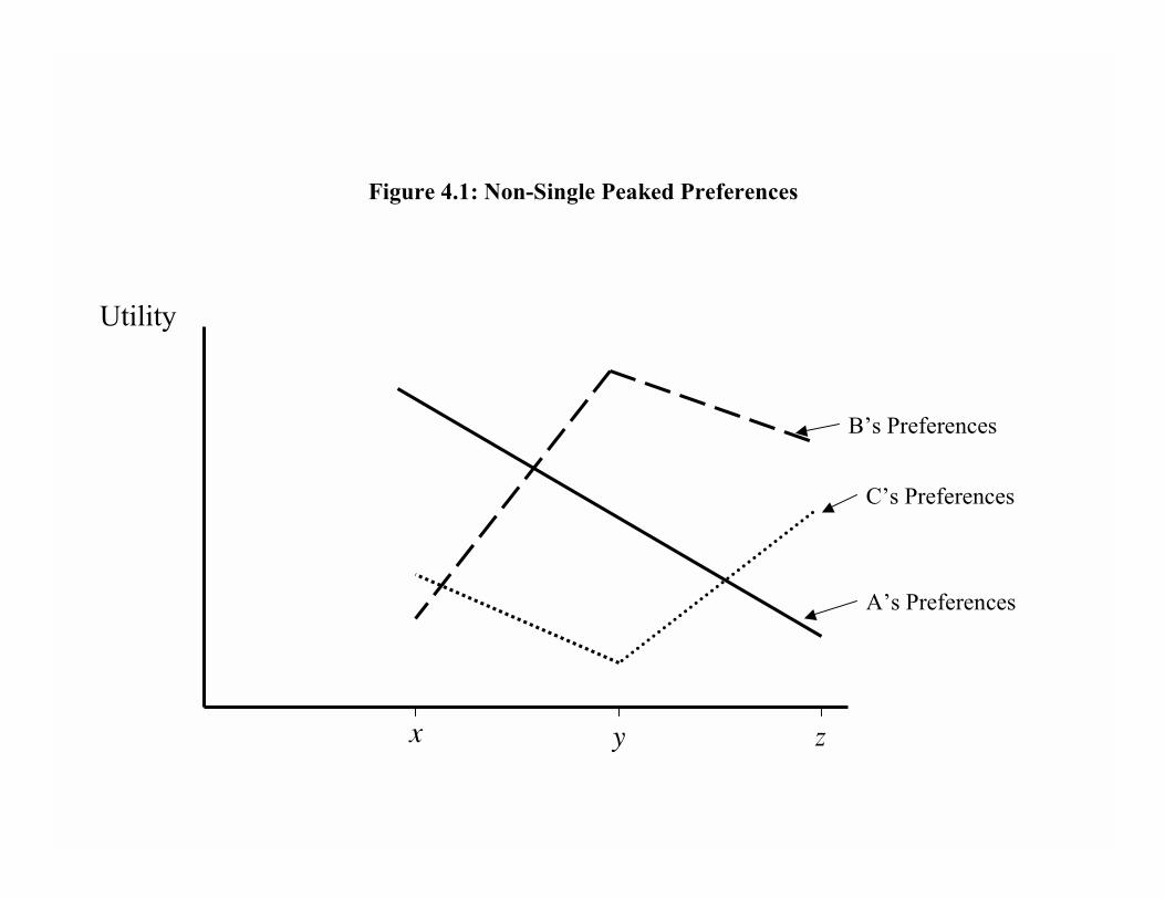
Figure 4.1: Non-Single Peaked Preferences

� � �

Utility

A�s Preferences

B�s Preferences

C�s Preferences

Figure 4.2: Single Peaked Preferences

� � �

Utility

A�s Preferences

B�s Preferences

C�s Preferences

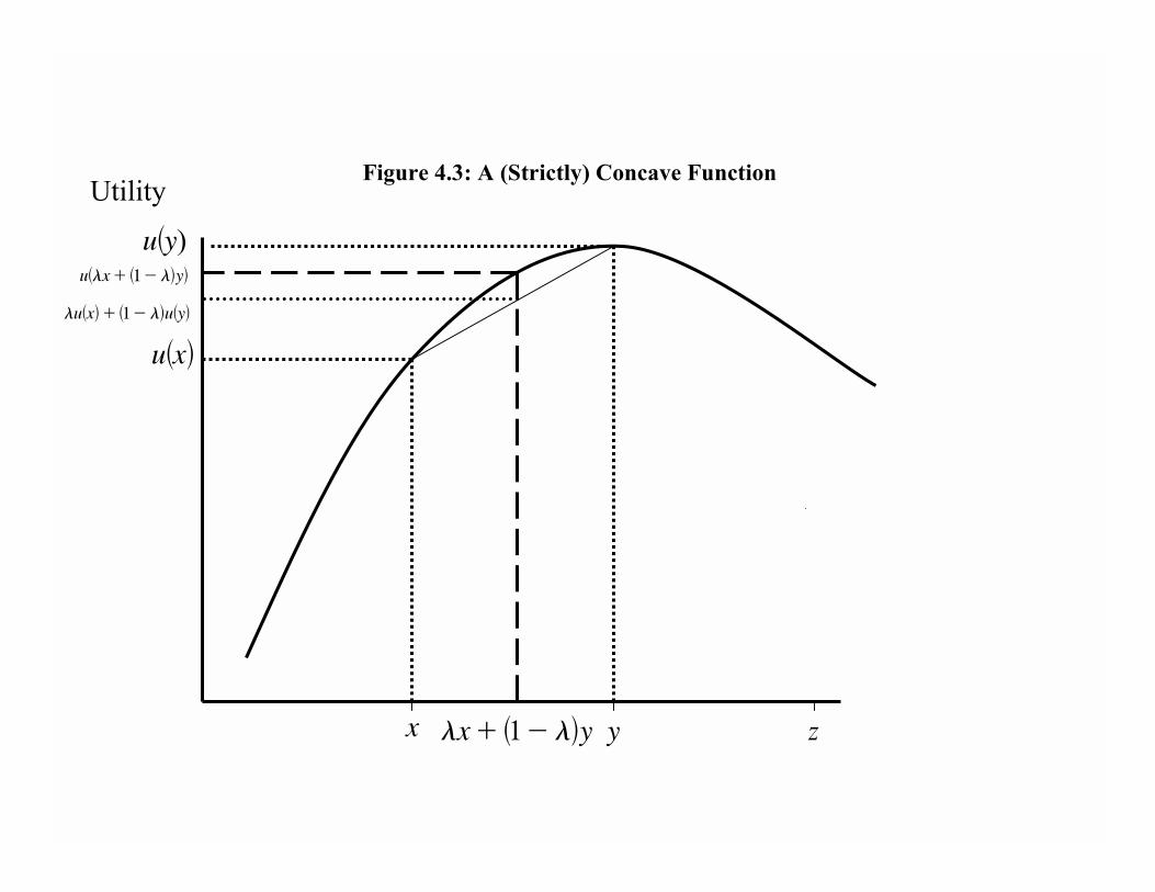
Figure 4.3: A (Strictly) Concave Function

� � �

Utility

����

�������

���)�����������

��������������

Figure 4.4: A (Strictly) Quasi-Concave Function

� � �

Utility

����

�������

����

�����������

Figure 4.5: A Function which is not Quasi-Concave

� � �

Utility

����

����

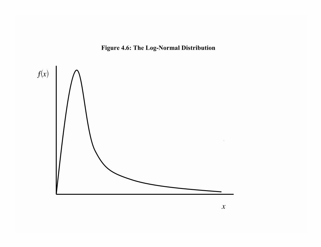
Figure 4.6: The Log-Normal Distribution

����

�