politecnico di torino porto institutional repository you for being around and fair. ... my dear...
TRANSCRIPT

Politecnico di Torino
Porto Institutional Repository
[Doctoral thesis] Preoperative Systems for Computer Aided Diagnosis basedon Image Registration: Applications to Breast Cancer and Atherosclerosis
Original Citation:Riyahi Alam, Mohamad Sadegh (2015). Preoperative Systems for Computer Aided Diagnosis basedon Image Registration: Applications to Breast Cancer and Atherosclerosis. PhD thesis
Availability:This version is available at : http://porto.polito.it/2592170/ since: February 2015
Published version:DOI:10.6092/polito/porto/2592170
Terms of use:This article is made available under terms and conditions applicable to Open Access Policy Arti-cle ("Creative Commons: Attribution 3.0") , as described at http://porto.polito.it/terms_and_conditions.html
Porto, the institutional repository of the Politecnico di Torino, is provided by the University Libraryand the IT-Services. The aim is to enable open access to all the world. Please share with us howthis access benefits you. Your story matters.
(Article begins on next page)

Preoperative Systems for Computer Aided Diagnosis based on Image Registration: Applications to Breast Cancer and Atherosclerosis
Mohamad Sadegh Riyahi Alam
Department of Mechanical and Aerospace Engineering Politecnico di Torino
Turin, Italy February 2015
Supervisors:
Filippo Molinari Alberto Audenino
Assistant Supervisors: Valentina Agostini Umberto Morbiducci
A dissertation submitted to Politecnico di Torino in partial fulfillment of the requirements for the degree of Doctor of Philosophy.
© 2015 Mohamad Sadegh Riyahi Alam

THIS PAGE WAS LEFT INTENTIONALLY BLANK

iii
to my beloved father and mother who
devoted their precious life for us
put us in more than we expected
taught us nothing but pureness

iv
Acknowledgment Before starting my PhD, Marta Peroni who taught me what is “Biomedical Engineering”, told me studying doctorate would be a good opportunity to face how to solve the problems “individually”. During my career, many times I had to inevitably overcome both scientific and daily problems relying on self-capabilities. However obviously, conquering obstacles would become easier each time after one learns how to organize the time and energy and how to control the “stress” to maintain the problems ahead. I was from away, so the first year must have been on self-proving to the engineering society of “Electronics and Mechanics” that their combination had emerged the group of “Bioengineers”, so that I would be able to fix my position somewhere there. I was assigned “two professors” from both societies in which after a while I learned it is quite “unusual”. In any case, I tried to tighten the nodes of both societies. Of course did not go well. I chose a project from the “Electronics” and deploying my abilities I was able to obtain an acceptable outcome “scientifically”. Sometimes, in your life something happens that you are forced to believe there might be a superior spiritual power. The second year ahead, I found a project in which “accidentally” it was “Biomechanics”. I was going to Nagoya. Days were hard-working but super-satisfying. I went back with good outcome, again “scientifically”. Eventually, probably I will be able to connect the nodes from two societies. That is a good outcome “non-scientifically”. Now I admit PhD is the best opportunity to learn problem solving, in which brings you up in your next career, raise your expectations and self-confidence. That is why it is called “Over-qualified degree”. The “conclusion” is that it was “assolutamente” worth it stepping into this society where the following people helped me partially or permanently to arrive to this point: Prof. Molinari, you made me comprehend how an excellent coordinator should be like. Indeed without your helpful comments and advices, I would not have been able to go forward all the way. Thank you for being around and fair. Prof. Audenino, I appreciate your short helpful advices during my both works, when I was stuck and confused with the new concepts. You really know everything. You have always been kind and smiling to me. Valentina, you know without your help I was not able to complete my works. You not only advised me on the projects but you also inspired me to keep moving forward. Grazie mille! Umberto, you always were there if I had to ask you something. Thank for your aspiration on hard-working. I appreciate all the members from both BioLab and my own office, Prof. Knaflitz, Prof. Balestra, Prof. Bignardi, Beppe (you are special!), Kristen, Issey, Valeria Chiono, and my dear friend Shady in which being right beside you was fun during more than half of my career. Thanks for energizing me. Both Giuseppi (Isu and Pisani), meeting you was the last best thing happened in my last year. Thanks for being around as good friends. Last but not least, my parents, my dear father and mother, I do not have any word to express my gratitude for your efforts and kindness to keep me motivated in this way. My father, your precious advices helped me to love my field of work. My dear lovely mother, your heart-warming patience gave me a huge support during the hard times in my way. Thank you both! Thank you all who helped me to finish this career with a complete confident, what I started with a doubt.

v
Abstract Computer Aided Diagnosis (CAD) systems assist clinicians including radiologists and
cardiologists to detect abnormalities and highlight conspicuous possible disease. Implementing a
pre-operative CAD system contains a framework that accepts related technical as well as clinical
parameters as input by analyzing the predefined method and demonstrates the prospective output.
In this work we developed the Computer Aided Diagnostic System for biomedical imaging
analysis of two applications on Breast Cancer and Atherosclerosis.
The aim of the first CAD application is to optimize the registration strategy specifically for
Breast Dynamic Infrared Imaging and to make it user-independent. Base on the fact that
automated motion reduction in dynamic infrared imaging is on demand in clinical applications,
since movement disarranges time-temperature series of each pixel, thus originating thermal
artifacts that might bias the clinical decision. All previously proposed registration methods are
feature based algorithms requiring manual intervention. We implemented and evaluated 3
different 3D time-series registration methods: 1. Linear affine, 2. Non-linear Bspline, 3. Demons
applied to 12 datasets of healthy breast thermal images. The results are evaluated through
normalized mutual information with average values of 0.70±0.03, 0.74±0.03 and 0.81±0.09 (out
of 1) for Affine, BSpline and Demons registration, respectively, as well as breast boundary
overlap and Jacobian determinant of the deformation field. The statistical analysis of the results
showed that symmetric diffeomorphic Demons registration method outperforms also with the
best breast alignment and non-negative Jacobian values which guarantee image similarity and
anatomical consistency of the transformation, due to homologous forces enforcing the pixel
geometric disparities to be shortened on all the frames. We propose Demons registration as an
effective technique for time-series dynamic infrared registration, to stabilize the local temperature
oscillation.
The aim of the second implemented CAD application is to assess contribution of calcification in
plaque vulnerability and wall rupture and to find its maximum resistance before break in image-
based models of carotid artery stenting. The role of calcification inside fibroatheroma during
carotid artery stenting operation is controversial in which cardiologists face two major problems
during the placement: (i) “plaque protrusion” (i.e. elastic fibrous caps containing early
calcifications that penetrate inside the stent); (ii) “plaque vulnerability” (i.e. stiff plaques with
advanced calcifications that break the arterial wall or stent). Finite Element Analysis was used to
simulate the balloon and stent expansion as a preoperative patient-specific virtual framework. A
nonlinear static structural analysis was performed on 20 patients acquired using in vivo MDCT
angiography. The Agatston Calcium score was obtained for each patient and subject-specific
local Elastic Modulus (EM) was calculated. The in silico results showed that by imposing
average ultimate external load of 1.1MPa and 2.3MPa on balloon and stent respectively, average
ultimate stress of 55.7±41.2kPa and 171±41.2kPa are obtained on calcifications. The study
reveals that a significant positive correlation (R=0.85, p<0.0001) exists on stent expansion
between EM of calcification and ultimate stress as well as Plaque Wall Stress (PWS) (R=0.92,
p<0.0001), comparing to Ca score that showed insignificant associations with ultimate stress
(R=0.44, p=0.057) and PWS (R=0.38, p=0.103), suggesting minor impact of Ca score in plaque
rupture. These average data are in good agreement with results obtained by other research groups
and we believe this approach enriches the arsenal of tools available for pre-operative prediction
of carotid artery stenting procedure in the presence of calcified plaques.
vi
Table of Contents Acknowledgment ............................................................................................................................ iv
Abstract............................................................................................................................................ v
List of Tables ................................................................................................................................. viii
List of Figures .................................................................................................................................. ix
Section 1: Computer Aided Diagnosis System for Breast Cancer Detection in Dynamic Area Telethermometry............................................................................................................................. 1
Chapter 1 : Introduction to Dynamic Area Telethermometry ......................................................... 2
1.1. Dynamic Area Telethemometry............................................................................................ 3
1.2. Problems and Aims of the work ........................................................................................... 6
1.3. CAD for breast cancer detection in IR imaging ..................................................................... 9
1.4. Time-series image registration ........................................................................................... 10
1.5. Registration evaluation methods ....................................................................................... 13
Chapter 2 : Methods and Implementation .................................................................................... 15
2.1. Data Acquisition .................................................................................................................. 16
2.2. Breast Segmentation .......................................................................................................... 17
2.3. DAT specific registration methods ...................................................................................... 18
2.3.1. Linear Affine registration ............................................................................................. 18
2.3.2. Nonlinear parametric Bspline registration .................................................................. 19
2.3.3. Symmetric diffeomorphic Demons registration .......................................................... 22
2.4. DAT Registration evaluation methods ................................................................................ 23
2.4.1. DAT specific Breast Boundary Overlap ........................................................................ 23
2.4.2. Normalized Mutual Information .................................................................................. 24
2.4.3. Jacobian determinant of the transformation .............................................................. 24
Chapter 3 : Results ......................................................................................................................... 27
3.1. Comparing the implemented methods .............................................................................. 28
3.2. Pre and Post Registration comparison ............................................................................... 30
3.3. Spectral analysis of temperature modulation .................................................................... 33
Chapter 4 : Discussion and Conclusion .......................................................................................... 36
4.1. Discussion ........................................................................................................................... 37
4.2. Conclusion .......................................................................................................................... 40
Section 2: Preoperative Computer Aided Diagnostic System for Carotid Artery Stenting simulation using Finite Element Analysis ...................................................................................... 42

vii
Chapter 5 : Introduction to Carotid Arterial Stenting .................................................................... 43
5.1. Calcified carotid atherosclerotic plaque and Agatston score ............................................. 44
5.2. Carotid Artery Stenting ....................................................................................................... 50
5.3. Material and Mechanical parameters ................................................................................ 52
5.3.1. Volume score ............................................................................................................... 53
5.3.2. Elasticity ....................................................................................................................... 53
5.3.3. Plasticity ....................................................................................................................... 54
5.4. Finite Element Method ....................................................................................................... 56
5.5. Problems and aims of the work .......................................................................................... 58
Chapter 6 : Materials and Methods ............................................................................................... 60
6.1. Data Acquisitions ................................................................................................................ 61
6.2. Calcification model reconstruction ..................................................................................... 61
6.2.1. Linear elasticity ............................................................................................................ 62
6.2.2. Nonlinear plasticity ...................................................................................................... 63
6.2.3. 3D Reconstruction ....................................................................................................... 64
6.3. Balloon/Stent model reconstruction .................................................................................. 67
6.3.1. 3D reconstruction ........................................................................................................ 69
6.4. Finite Element Analysis and Simulation .............................................................................. 69
Chapter 7 : Results ......................................................................................................................... 74
7.1. Arterial Diversity ................................................................................................................. 75
7.2. Plaque imposed by Balloon ................................................................................................ 76
7.3. Plaque imposed by stent .................................................................................................... 80
Chapter 8 : Discussion and Conclusion .......................................................................................... 88
8.1. Comparison of loads imposed by balloon and stents ......................................................... 89
8.2. Calcium score ...................................................................................................................... 90
8.3. Area and Volume score....................................................................................................... 94
8.4. Penetration and protrusion ................................................................................................ 94
8.5. Ultimate External Pressure ................................................................................................. 94
8.6. Tangent Modulus ................................................................................................................ 94
8.7. Conclusion .......................................................................................................................... 95
Bibliography ................................................................................................................................... 96
Curriculum Vitae .......................................................................................................................... 100
Publications ................................................................................................................................. 105

viii
List of Tables Table 2.1. Classification of cost function exploited for implemented linear and nonlinear
registration methods. ..................................................................................................................... 20 Table 2.2. Most optimized registration parameters in order to register the 500 frames of thermal breast images. For registering each frame it takes 2 seconds, thus for 500 frames it takes 16 minutes on Intel Centrino 2 core 2.27 GHz CPU and 3GB RAM PC. ............................... 21 Table 2.3. Registration parameters. Registrations are performed with Intel Core 2Duo 2.27 GHz CPU, 3GB RAM. a[linear level, non-linear level], b(coarse stage, fine stage). ................................ 22 Table 3.1. Quantitative numerical values resulted from each registration method are presented
here for every subject. Average NMI and BBO values obtained from all the frames of each
subject proves that Demons method is pioneer in terms of both similarity of the warped frames as
well as smoothness of DF indicated by absence of negative Jacobian value. Likewise, small value
for standard deviation in the Demons method obtained from all the metrics proves that diversity
in the results is very small. AAffine,
bBspline,
cDemons ............................................................... 28
Table 3.2. Intra-subject and inter-subject overall results obtained from registration methods on all the cases. .................................................................................................................................. 30 Table 6.1. Material properties belong to all the calcifications in this study ordered from the highest to the lowest Ca score. patient-specific elastic modulus and density are also presented. ....................................................................................................................................................... 63 Table 6.2. Utilized material properties for artery, balloon and two stents. .................................. 68 Table 6.3. Clinical information belonging to all the patients. ........................................................ 68 Table 7.1. Average mechanical parameters from balloon simulation and their correlation with elastic modulus. (statistically significant threshold, p<0.05) ......................................................... 77 Table 7.2. Mechanical parameters obtained for each patient by imposing balloon on the calcified plaque. ........................................................................................................................................... 78 Table 7.3. Average values for mechanical parameters obtained from stent simulation and their nonlinear spearman’s correlation with elastic modulus. (statistically significant threshold, p<0.05). .......................................................................................................................................... 80 Table 7.4. Mechanical parameters obtained for each patient by imposing balloon on the calcified plaque. ........................................................................................................................................... 82 Table 8.1. Mechanical parameters obtained from Stent simulation and their nonlinear spearman’s correlation with Ca Score. (statistically significant threshold, p<0.05)...................... 91

ix
List of Figures Figure 1.1. The electromagnetic spectrum and the IR region. ........................................................ 3 Figure 1.2. General procedure of a DAT starting from patient acquisition, segmentation of breast region, registration of corresponding pixels on time temperature series and converting the signal to frequency domain followed by computation of PSD over specific frequency. ................. 4 Figure 1.3. Problem exists in DAT procedure during patient acquisition leading to misalignment of the temperatures along the frames. ........................................................................................... 7 Figure 1.4. (a) Traditional Landmark placement on the breast for manual feature based registration. (b)Thermogram obtained with landmarks on the breast. .......................................... 7 Figure 1.5. (a) Final PSD spectral image obtained after placing the landmarks. (b) Smoothed spectral image obtained without landmark deploying an automated registration. ....................... 8 Figure 1.6. DF as outcome of registration process has been overlaid on fixed images belonging to current frame of one of our subjects. Parts of the body with burden of vectors represent a large movement of the patient during DAT acquisition process. ........................................................... 11 Figure 1.7. The whole procedure of the image registration [12]. ................................................. 12 Figure 2.1. Current frame belonging to all the subjects are presented. Each subject is acquired
three times, hence in total we are provided with 12 datasets in order to analyse movement of the
body through image registration and further spectral analysis. ..................................................... 16 Figure 2.2. Thermal breast segmentation done using edge based method in [12]. ........................ 17 Figure 2.3. General concepts of Affine registration in which the transformation functions consist of only linear transformation. ....................................................................................................... 18 Figure 2.4. Each control points acts as an automated marker on the image. Since it is polynomial it can be derived to N times, and well fits the optimization functions. Number of control points affects the level of registration from coarse to fine grid level. Therefore, it covers the local motion. .......................................................................................................................................... 20 Figure 2.5. First, velocity field is obtained using gradient symmetric forces that is applied on the moving frames to compensate the dissimilarities. Gaussian smooth kernel is deployed as additional regularizer. Fits for time-series sequential thermal registration. ................................ 22 Figure 2.6. A schematic view of how to obtain Breast Boundary Overlap as one of the DAT specific evaluation metrics is depicted. C.O.M stands for centre of mass which are calculated for the whole image and each left and right breasts. ......................................................................... 24 Figure 2.7. Volume increase, decrease and no volume change after evaluating Jacobian
determinant of the final deformation. [33] .................................................................................... 26 Figure 3.1. In order to perform a Post-hoc analysis for nonparametric Friedman test (P<0.001, df
= 2), box plots representing distribution of errors on the obtained results from provided metrics
for all the methods (inter-subject evaluation) are presented. The analysis shows there is a critical
difference in the groups of Demons method for every experiment acting as the best method in our
experiments. ................................................................................................................................... 29 Figure 3.2. Case variation error on all the methods performed on all the cases. ......................... 29 Figure 3.3. BBO metric is used to evaluate and compare each method applied before (blue line)
and after (red line) registration for every frame belonging to Subject 1 (top row) and Subject 2
(bottom row). X axis represents number of frames from 1 to 476 and Y axis represents BBO error
values (smaller better). Evaluated methods are presented as Affine, Bspline and Demons
respectively from left to right for panels (a), (b) and (c). Demons method shows the lowest
differences error for BBO comparing to other methods. ............................................................... 31

x
Figure 3.4. Same as Fig. 3.3, here NMI metric is used to evaluate and compare each method
applied before (blue line) and after (red line) registration for every frame belonging to Subject 1
(top row) and Subject 2 (bottom row). X axis represents number of frames from 1 to 476 and here
Y axis represents NMI values (larger better). Evaluated methods are presented as Affine, Bspline
and Demons respectively from left to right for panels (a), (b) and (c). NMI values for Demons
registration is the highest comparing to the others, and the values for each frame is stable. ........ 32 Figure 3.5. Final 2D spectral image obtained from PSD values of each pixel without (a) and with
(b) registration. High frequency components of the temperature values for every pixel is shown as
darker red and low frequency component with lighter blue. Unnecessary noises are removed after
registration (b), leading to a smoother image that helps in the further diagnosis. ......................... 34 Figure 3.6. Time-temperature series of an arbitrary spot in Subject1-case1 belonging to before (a)
and after (b) registration. Acquisition time is 10s and vertical axis for panel (b) has been
magnified in order to emphasis that the scale of temperature variation is smaller after registration.
....................................................................................................................................................... 35 Figure 3.7. PSD-frequency graph of the latter time-temperature series for with (red) and without (blue) registration are overlaid. As expected, frequency range is limited between 0.1 and 1 Hz and PSD values for the registered signal has lower peak thus more stabilized comparing to non-registered curve. ............................................................................................................................ 35 Figure 4.1. DF overlaid on warped images belonging to current frame of Subject1-case1, in order to show the smoothness of final DF yielded for each method. Demons resulted with the least irregularity in DF along with the shortest vectors of displacements proving that misalignment of the warped frames is well compensated. ..................................................................................... 38 Figure 4.2. Obtained Power Spectral Density and frequency series of a random point comparing the stabilization before (b) and after the registration (a). ............................................................ 39 Figure 5.1. Schematic representation of an elastic artery. Adapted from Rhodin [9]. ................. 44 Figure 5.2. Many parts and sections of carotid arteries, in addition to plaque build-up progression inside the artery. ........................................................................................................ 46 Figure 5.3. Progression of atherosclerotic disease. From the initial state, where LDL migrate through the endothelium in the intima (left side) to the beginning of intima thickening (right side). Illustration adapted from [44]. ............................................................................................ 46 Figure 5.4. Calculation of plaque volume in a step-by-step fashion using the software and
measurement of percent stenosis is demonstrated. (a) Manually drawn region of interest for
sculpting is depicted on the coronal maximum intensity projection (MIP) image. (b) Calcified
plaque on the sculpted MIP. (c) Volume rendered appearance of the plaque with automatic
calculation of calcified plaque volume with a single button click, calculated to be 0.25cm3 in this
patient. (d) Calculation of percent stenosis on lateral view of carotid digital subtraction
angiography. .................................................................................................................................. 48 Figure 5.5. Stepwise relationship between Hounsfield units and the calcium density score as they
relate to the determination of the Agatston score. ......................................................................... 49 Figure 5.6. Real size and shape of an angioplasty stent that is a small tube mesh. ...................... 51 Figure 5.7. (a)Angioplasty balloon inserted by the catheter is depicted inside the artery to push the plaque. (b) the whole procedure of carotid artery stenting is illustrated by a closed-cell stent. ....................................................................................................................................................... 51 Figure 5.8. A general stress-strain curve that demonstrates elastic and plastic/linear and nonlinear
domains of a parameter. ................................................................................................................. 52 Figure 5.9. (a) Depicts the main principle of Young’s modulus (Elastic modulus) and (b)
Poisson’s ratio. ............................................................................................................................... 53

xi
Figure 5.10. Stress-Strain curve belong to (a): Patient 1, (b): Patient 2, (c): Patient 3, (d): Patient 4.
....................................................................................................................................................... 55 Figure 5.11. The broad procedure of FEM starting from segmentation part, in which the artery is segmented from a CT image. Afterwards, the geometry is structured and volumes are shaped in which the bodies are ready for the assembly part. ....................................................................... 57 Figure 5.12. A general scheme of a post processing analysis of a FEM simulation as an example. In this sample analysis von mises pressure of the stent expansion is depicted inside the carotid artery. ............................................................................................................................................ 57 Figure 5.13. (a) When the stent is too much open, the plaque is smashed and penetrated into the stent leading to plaque protrusion. (b) When the stent is expanding, hardness of the plaque prevents the stent to open completely leads to plaque and arterial vulnerability. ...................... 59 Figure 6.1. Stress-strain curve belong to calcification of case 1. σy is yield stress that plastic deformation begins. EM (E) and TM (Et) have been pointed along with εe and εp that represent elastic and plastic strain. ............................................................................................................... 63 Figure 6.2. Segmentation and 3D reconstruction of the artery and the calcification without volume. .......................................................................................................................................... 65 Figure 6.3. Connecting the meshes belonging to calcification and the artery in Rhinoceros. ...... 66 Figure 6.4. Assembly of two stent models resided on the calcification inside the artery using a specific geometry........................................................................................................................... 66 Figure 6.5. Assembled layout belongs to a case in which the stents is resided on the calcification inside the artery............................................................................................................................. 67 Figure 6.6. Sterling Balloon (A) and two stents: Closed-cell Wallstent (B) and Open-cell Precise
(C) three dimensional design. ........................................................................................................ 69 Figure 6.7. CT image belongs to a case where left carotid artery along with the calcifications are visible. Both artery and the calcified plaque are segmented for further construction in coronary (a), saggital (b) and axial view (c). ................................................................................................. 70 Figure 6.8. Mesh view of balloon placed on calcification for Case C4. (a)Finer mesh size is utilized for the calcification where (b)Coarser meshing has been defined for calcification. Mesh element size for balloon is coarser comparing to calcification due to priority in importance of the objects in the analysis. Contacts area has the same mesh configuration. ............................. 71 Figure 6.9. (a) Cartesian coordinate system (b)Cylindrical coordinate system ............................. 72 Figure 6.10. Geometrical properties of the modeled balloon and stents are presented. External Carotid Arteries (ECA) and Internal Carotid Arteries (ICA) are shown along with the calcification resided in the entry of ICA. Panel (A) shows pre-dilation balloon placed on calcification and in Panel (B) designed closed-cell Wallstent is presented. In Panel (C) open-cell Precise stent is fixed on a case with particular calcification. .......................................................................................... 72 Figure 6.11. Loading condition defined on the inner surface of the stent to be pushed and opened. The force is imposed on the x direction of the cylindrical coordinate in this case. The force has been obtained through an approximation of guidance pressure multiplied by the cross-sectional area and by using trial and error it has been finally determined for each case and it is case specific............................................................................................................................. 73 Figure 7.1. Overall coronal mesh view of the segmented arteries and calcification from CT images belonging to 12 cases out of 20 cases. Yellow objects express calcifications. .................. 76 Figure 7.2. Scatter plot for EM v.s. ultimate stress and PWS for balloon analysis. Quadratic regression curves are also depicted to fit the intercepts. Strong positive correlation is inferred from the graph. .............................................................................................................................. 77

xii
Figure 7.3. Mechanical parameters of (a)ultimate stress (b)PWS(c)Elastic strain(d)Deformation(e)Plastic strain(f)standardized Ca score and ultimate stress for 12 cases imposed by balloon. ...................................................................................................................... 79 Figure 7.4. Scatter plot for EM v.s. ultimate stress and PWS for stent simulation. Quadratic regression curves show better data fit for stent analysis whereas comparing to balloon expansion monotonic pattern is well demonstrated. ................................................................... 81 Figure 7.5. Mechanical parameters of (a)ultimate stress (b)PWS(c)Elastic strain(d)Deformation(e)Plastic strain for 12 cases imposed by stents. ........................................ 83 Figure 7.6. Stress-strain analysis for C4. Panel A shows Von mises stress distributed over the surface of the calcified plaque. Expanded balloon is pointed along with the ICA, ECA and wall thickness. Panel B represents elastic strain. Left color bar for strain distribution corresponds to the maximum values in Table 7.4. Panel C belongs to nonlinear plastic deformation occurred in the center of dynamic interaction between balloon and calcification. ........................................ 84 Figure 7.7. Stress-strain analysis belongs to C10. Panel A represents Von mises stress distribution due to wallstent expansion which has been pointed. Panel B shows WSS on the arterial wall. In panel C we presented plaque and stent break due to stiffness of the calcification in which causes to cross the UTS and fail. ..................................................................................... 84 Figure 7.8. Stress-strain analysis of three different cases imposed by balloon and stent. Panel (A)
shows equivalent stress from center of the calcification while pressed by closed-cell stent. Panel
(B) demonstrates PWS of a calcification on balloon case and Panel (C) represents plastic-strain
imposed by closed-cell stent on a case. ......................................................................................... 85 Figure 7.9. Plaque protrusion and rupture are simulated by inducing the ultimate pressure on the
stents. Panel (A) shows the plaque is penetrated inside the stent. Panel (B) and (C) demonstrate
soft plaque break due to 140kPa and 30kPa of the ultimate stress that crossed the maximum
resistance of the calcification......................................................................................................... 86 Figure 7.10. (a)Equivalent Von mises stress on the Plaque wall being pushed by the balloon.
(b)PWS on a plaque in the middle of lumen. (c)stress on the calcified plaque imposed by balloon.
....................................................................................................................................................... 87 Figure 8.1. Graphs representing comparisons of obtained mechanical parameters imposed by balloon and the stents. (a) Stresses (b)Elastic strain (c)PWS and (d) Plastic strain. ...................... 90 Figure 8.2. Scatter plot showing weak correlation of Ca score and ultimate stress of calcifications
obtained for balloon and stent simulations. ................................................................................... 91 Figure 8.3. Comparisons of Ca score in correlation with Volume score, HU and elastic modulus. Panel (a) shows only EM belongs to 12 cases, (b) proportion of Ca score and HU, (c)corralation between Ca score and volume score and (d)shows standardized values for Ca score and EM for the sake of seeking the relations. .................................................................................................. 93

1
Section 1: Computer Aided Diagnosis System for Breast Cancer Detection in Dynamic Area Telethermometry

Chapter 1– Introduction to Dynamic Area Telethermometry
2
Chapter 1 : Introduction to Dynamic Area Telethermometry

Chapter 1– Introduction to Dynamic Area Telethermometry
3
1.1. Dynamic Area Telethemometry
Early detection of breast cancer has been shown to be crucial for the survival of the patients [1].
Dynamic Area Telethermometry (DAT) has been explored as a potential complementary
technique with respect to mammography. The basic assumption is that normal tissues show
temperature modulation that is different from cancerous tissue [2]. The surface temperature
modulation caused by cancer, occurs at specific frequencies [2], [3]. Hence, the spectral analysis
of the time variations of the local temperature could allow for non-invasively detecting cancerous
lesions.
In general, IR radiation covers wavelengths that range from 0.75𝜇m to 1000µm, among which
the human body emissions that are traditionally measured for diagnostic purposes only occupy a
narrow band at wavelengths of 8µm to 12µm [4]. This region is also referred to as the Long-
Wave IR (LWIR) or body infrared rays. Another terminology that is widely used in medical IR
imaging is Thermal Infrared (TIR), which, as shown in Figure 1.1, covers wavelengths beyond
about 1.4µm. Within this region, the infrared emission is primarily heat or thermal radiation, and
hence the term thermography. The image generated by TIR imaging is referred to as the
thermogram. The Near Infrared (NIR) region occupies wavelengths between 0.75µm and 1.4µm.
The infrared emission that we observe in this region is not thermal [4]. Although the NIR and
Mid-Wave IR (MWIR) regions are not traditionally used in human body screening, the new
generation detectors have enabled the use of multispectral imaging in medicine, in which both
NIR [5] and MWIR [5] are observed in different diagnostic cases.
Figure 1.1. The electromagnetic spectrum and the IR region.
A general DAT procedure starts with a thermal camera generating consecutive 2D frames of the
patient’s breasts, reconstructed as 3D thermograms. Then all the frames are segmented in order to
remove artifacts and reduce the computational time. 3D time-series frame registration is
performed to eliminate the movement by aligning the corresponding pixels of each frame.
Eventually, the time-temperature series of each pixel during the time interval of acquisition is
obtained and transformed to the frequency domain to measure the modulation of the temperature.
More specifically, the Power Spectral Density (PSD) of the time-temperature signal is obtained
for each pixel. Then, the power in a specific frequency band is calculated obtaining a single final
image. Figure 1.2 shows the whole procedure.

Chapter 1– Introduction to Dynamic Area Telethermometry
4
In eventual spectral analysis of the dynamic infrared imaging for breast cancer diagnosis, motion
reduction of the patient is necessary, since it is combined with the signal of interest acting as the
noises. Therefore, motion reduction on the frames of thermogram is crucial. In our previous work
[9], a feature-based registration was applied on breast dynamic thermograms using a linear
piecewise polynomial transformation function with linear interpolation technique in order to
compensate the patients movements. However, there are certain drawbacks in feature-based
registration such as difficulty in placing the markers manually on the patient during the
acquisition as well as obtaining the optimal number of markers, necessity of additional prior
marker detection algorithms, limitation on choosing types of registration transformation function/
interpolation techniques/similarity metric and optimization method. Therefore, performing
automated intensity based motion reduction methods on the sequence of frames as well as
landmark-based registration by taking the criteria concluded in the previous article into the
account and annotating the landmarks on the dataset automatically, we can intensively facilitate
the whole acquisition process and dramatically advance the registration routine by choosing the
best suited method in motion compensation for DAT modalities. Clinical information is obtained
by analyzing in the frequency domain the small temperature fluctuations taking place in
numerous breast areas constituted by a few pixels.
Malignant cells release a chemical into the surrounding area called nitric oxide (NO), causes to
keep the existing blood vessels open (vasodilation), which awake the inactive cells and create
new one [6]. This is called angiogenesis and since malignant/aggressive and benign/normal
tissues have different infrared signals and temperature and physiological cardiovascular activities,
due to activities such as angiogenesis which is crucial for a tumor cell, hence thermo cameras can
be used to identify the latter activities and depict the temperature map predefined as Hot Spots
(final spectral image). The harmonic analysis of the time course of temperature fluctuations
allows obtaining information on the local blood perfusion using specific characteristics of the
vasculature supplying blood to the tumor, and the altered metabolism of cancerous tissue. In
literature, it has been reported that temperature fluctuations have an important diagnostic value in
oncology. [6]
Figure 1.2. General procedure of a DAT starting from patient acquisition, segmentation of breast region, registration of
corresponding pixels on time temperature series and converting the signal to frequency domain followed by
computation of PSD over specific frequency.

Chapter 1– Introduction to Dynamic Area Telethermometry
5
In this work the breast regions in all frames are masked out and segmented from the background
area, using a semi-automated algorithm developed by N. Scales et al [10] that employs Canny
edge detection and the Hough transform to detect the symmetric breast boundaries and isolates
the region of interest. Breast segmentation was checked and altered where necessary using
algorithm embedded in 3D Slicer software based on multiple label mapping and Otsu’s
thresholding, hence only body and breast region is registered and evaluated which helps in
computational time and the accuracy of the algorithm. Unsharp masking filtering is applied on
the images prior to evaluation to negate the noise and smoothness effect of interpolation.
DAT as a new modality can be deployed to detect the breast cancers relatively close to the
surface of the body. In a DAT detection examination, depending on the frame rate of the thermal
camera as the sampling frequency, several frames are acquired from the patient during a certain
amount of time. Based on Nyquist frequency, the sample rate of up to twice larger than the
chosen frequency band is sufficient. However depending on the limitation of the camera, the
more sampling frame rate one chooses, the obtained preliminary information is consecutive and
reliable. The perfusion frequency of the breast region is very low ranged from 0.1 to 1 Hz
(considering the ambient frequencies banded up to 6 Hz) mainly belonging to cardiogenic and
vasomotor frequencies [2], [3]. DAT is based on the assumption that normal tissues radiate
different temperature fluctuations, comparing to the malignant tissues due to the activities such as
angiogenesis [1]. DAT framework is proposed as following: first the infrared intensity versus
time series function at each pixel of the sequential frames is obtained and using PSD of the time-
series, the average integrated power distributed over the banded temperature frequency is
calculated. Finally the integrated outcome value is mapped into each pixel of a 2D thermal map
image.
Prior to spectral analysis of the signal of interest for the clinical evaluation, superimposed noise
signal emerged by the patient movement must be distinguished and eliminated and the sequential
dynamic frames must be registered. The movement during the consecutive dynamic frames,
disarrange the time-temperature series of each pixel, causing to false positive in the eventual
thermal map evaluation.
Section 1 of this thesis is organized as follows:
Chapter 1 introduces the major functionality of DAT framework as a complementary modality
for breast acquisition and cancer detection along with the problems we defined and the goal of
the research. Moreover the general concepts on image registration methods are presented as well
as evaluation of image registration methods.
In Chapter 2, we introduced our novel method of 3D time series registration methods in which
they are utilized for patient movement reduction. Then the DAT specific registration evaluation
methods are introduced along with data acquisition procedure.
Chapter 3, we show the results of our methods along with pre and post registration comparisons.
Then we use spectral analysis of temperature modulation on time temperature series as one DAT
specific evaluation method.
Finally in Chapter 4 we state the discussion followed by the eventual conclusion.

Chapter 1– Introduction to Dynamic Area Telethermometry
6
1.2. Problems and Aims of the work
A major problem exists during a DAT examination. While acquiring several frames of patients’
breasts, the movements disarrange the time-temperature series of each pixel, thus originating
thermal artifacts that might lead to a false positive or false negative in the final spectral image
used for diagnosis. Therefore, prior to spectral analysis, the patient movement must be
compensated and the sequential frames must be aligned using a 3D time-series registration
method [4].
We proposed an automated framework which after acquiring the thermal images, segments the
breast region of interest using non-interventional automated method and registers the thermal
frames to realign the sequence of images in order to attenuate the frequency difference of the
same corresponding pixels which represents the fluctuations in the temperature as well as to
compensate the patients’ movements during the acquisition. Finally by performing a thermal
frequency spectral analysis on the sequence of images, we obtain the spectral image in order to
perform estimations on detecting the suspicious cancerous regions.
In the literatures, many probes on registering static visible and infrared image have been
performed, however very few methods are proposed on automated real-time motion reduction in
sequential dynamic infrared frames especially in breast cancer detection. The most relevant
research is presented by [8] where the final aim is to detect the breast cancer tissue by performing
combination of several spatial and frequency filtering methods in order to increase the signal-
noise ratio on the sequence of 1200-1700 frames, acquired by 50 and 70 Hz frame rate of 24s
breath-holding images. However the movement of the patient is neglected as a prior-stabilization
process and the algorithms are performed by using Matlab, not suited for a real-time application.
In all of the similar works movement of the patient as a noise is either neglected or a breath-hold
process is supposed as assumption where in the 10-30s acquisition process, hardly can be
expected from the patient. Likewise in the very few previous attempts, no elaboration has been
made in terms of complete technical aspects of the frame registration.
In our previous work [9], a feature-based registration was applied on breast dynamic
thermograms using a linear piecewise polynomial transformation function with linear
interpolation technique in order to compensate the patients movements. However, there are
certain drawbacks in feature-based registration such as difficulty in placing the markers manually
on the patient during the acquisition as well as obtaining the optimal number of markers,
necessity of additional prior marker detection algorithms, limitation on choosing types of
registration transformation function/ interpolation techniques/similarity metric and optimization
method. Therefore, performing automated intensity based motion reduction methods on the
sequence of frames as well as landmark-based registration by taking the criteria concluded in []
into the account and annotating the landmarks on the dataset automatically, we can intensively
facilitate the whole acquisition process and dramatically advance the registration routine by
choosing the best suited method in motion compensation for DAT. Figure 1.3 depicts the
problem of misalignment of the pixels in the sequential consecutive frames of DAT.

Chapter 1– Introduction to Dynamic Area Telethermometry
7
Figure 1.3. Problem exists in DAT procedure during patient acquisition leading to misalignment of the temperatures
along the frames.
Image registration is the process of defining the transformation between two images so that the
coordinates in one image correspond to those in the other. Depending on the type of
transformation function, it is referred to as linear or deformable registration [5].
Very few methods were proposed for dynamic infrared images registrations, all were
concentrated on manual feature-based motion reduction [6], [7], [8]. In these methods several
markers are located on the region of interest of patient’s breast skin before the acquisition. The
markers are then recognized and used to construct the transformation function obtaining the
displacement to be compensated. In a previous work from our team [9], [10] a marker-based
registration was applied on breast dynamic thermograms. However, this technique had some
drawbacks: i) it was cumbersome to manually place the markers; ii) the registration was
dependent on the number of markers; iii) detection algorithms were needed to accurately locate
the centroid of each marker; iv) there were limitations on choosing types of registration
parameters. Figure 1.4 shows the landmark placement on the breast in order to follow the manual
feature based registration method. These points of the landmarks are utilized as a transformation
function for patient reduction methods. Figure 1.4 (b) shows the thermogram of the same image
in which the landmarks are completely visible as noises on the image that interrupt the final
decision.
(a) (b)
Figure 1.4. (a) Traditional Landmark placement on the breast for manual feature based registration. (b)Thermogram
obtained with landmarks on the breast.

Chapter 1– Introduction to Dynamic Area Telethermometry
8
(a) (b)
Figure 1.5. (a) Final PSD spectral image obtained after placing the landmarks. (b) Smoothed spectral image obtained
without landmark deploying an automated registration.
Figure 1.5 panel (a) shows final spectral image with landmarks placed on the breast region in
which ruined the image by noises and misleads the radiologists in diagnosis of the suspicious
spots. On the contrary in panel (b), by deploying automated registration method without
landmarks, we can obtain a smooth final PSD image which helps the radiologists to clearly focus
on vulnerable spots only.
The purpose of this paper is to implement and test different types of marker-less linear and non-
linear intensity based registration methods (which we implemented in ITK [11]) on the healthy
subjects of dynamic time series breast infrared images, in order to obtain the best suited
registration method along with optimization of DAT registration parameters.
We developed Affine linear registration along with Bspline and Demons nonlinear 3D time-series
registration method by minimizing the spatial displacement of the corresponding points on the
images. Performance of the methods was evaluated using assessment of DAT specific symmetric
alignment of breast boundary followed by image similarity measurement using Normalized
Mutual Information (NMI) and eventually Jacobian determinant of the transformation. All the
methods are performed automatically without human intervention.
DAT motion compensation evaluation is crucial since, there are huge amount of works that have
been done on evaluating different registration techniques on different current state of the art
modality dataset of different parts of body e.g. Brain CT/MRI, Xray-mammography, head and
neck, pulmonary CT, Prostate etc. taking into account the physiological/anatomical motion
properties, in order to obtain an optimal compensation of the excess movement. However, there is
no work having done on evaluation and comparison of different registration methods on time
series frames of dynamic thermograms. Despite the latter medical modalities which two different
mono/multi-modalities images are used as fixed and moving image to perform the registration
algorithm, in this field of work, different slices/frames inside one 3D image/thermogram should
be aligned on eachother, taking into account the first frame as fixed image and all the rest
sequential frames as the moving image. This fact brings the automated intensity based
registration into a new challenge. This process of “Time-series registration” is on the demand of
the developers in this field of work, since it has not been introduced before in any open source
software society and it is considered as a novelty.

Chapter 1– Introduction to Dynamic Area Telethermometry
9
1.3. CAD for breast cancer detection in IR imaging
According to American Cancer Society's report on Cancer Facts and Figures [12], breast cancer is
the most commonly diagnosed cancer in women, accounting for about 30 percent of all cancers in
women. In 2004, approximately 215,990 women in the United States receive a diagnosis of
invasive breast cancer and 40,110 die from the disease. Figure 2 shows the growth in estimated
new breast cancer cases in women since 2001. On the other hand, research [12] has shown that if
detected earlier (tumor size less than 10mm), the breast cancer patient has an 85% chance of cure
as opposed to 10% if the cancer is detected late. Other research also shows evidence of early
detection in saving life [17], [18]. Many imaging modalities can be used for breast screening,
including mammography using X-ray, IR, MRI, CT, ultrasound, and PET scans. Although
mammography has been the base-line approach, several problems still exist that affect the
diagnostic accuracy and popularity. First of all, mammography, like ultrasound, depends
primarily on structural distinction and anatomical variation of the tumor from the surrounding
breast tissue [18]. Unless the tumor is beyond certain size, it cannot be imaged as X-rays
essentially pass through it unaffected. Secondly, the mammogram sensitivity is higher for older
women (age group 60-69 years) at 85% compared with younger women (<50 years) at 64% [18]
whose denser breast tissue makes it more difficult for mammography to pick up suspicious
lesions. Thirdly, patients gone through mammography screening are exposed to X-ray radiation
which can mutate or destroy the tissue they penetrate. A new study in the British medical journal
[19] shows that screening actually leads to more aggressive treatment, increasing the number of
mastectomies by about 20% and the number of mastectomies and tumorectomies by about 30%.
Finally, mammography is relatively expensive nowadays and is less convenient to take. Even
though other modalities like MRI and PET scan could provide valuable information to diagnosis,
they are not popularly adopted for various reasons including high cost, complexity and
accessibility issues [19]. Compared to mammography, MRI, CT, ultrasound, and PET scans
which are also called the after-the-fact (a cancerous tumor is already there) detection technologies,
IR imaging is able to detect breast cancers 8-10 years earlier than mammography [18], [19]. In
[20] reported that the average tumor size undetected by IR imaging is 1:28cm vs. 1:66cm by
mammography. In addition, IR imaging is non-invasive, non-ionizing, risk-free, patient-friendly,
and the cost is considerably low. These features, together with its early detection capability, have
enabled IR imaging a strong candidate for complementary diagnostic tool to traditional
mammography.
Computer-aided diagnosis (CAD) has been playing an important role in the analysis of IR images,
as human examination of images is often influenced by various factors like fatigue, being careless,
etc. The detection accuracy is also confined by the limitations of human visual system. On top of
all these factors, a shortage of qualified radiologists also put an urgent demand on the
development of CAD technologies. Currently, research on smart image processing algorithms on
IR images tends to improve the detection accuracy from three perspectives: smart
image enhancement and restoration algorithms, asymmetry analysis of the thermogram including
automatic segmentation approaches, and feature extraction and classification.
All objects with a temperature above absolute zero (-273 K) emit infrared radiation from their
surface. The Stefan-Boltzmann law, also known as Stefan's law, states that the total energy
radiated per unit surface area of a blackbody in unit time (blackbody irradiance), is directly
proportional to the fourth power of its absolute temperature. This law can be mathematically
expressed as:

Chapter 1– Introduction to Dynamic Area Telethermometry
10
𝐸 = 𝜎𝑇4 (Equation 1.1)
where
E = total emitted radiance in W/m2
σ = 5.6697 × 10⁻⁸ W m-2
K-4
(Stefan-Boltzmann constant)
T = absolute temperature of the emitting material in Kelvin.
In order to maintain a constant temperature within the human body, the excess heat produced
during metabolic activity is dissipated in part, in the form of infrared radiation. The wavelength
of the radiation that leaves the surface of the skin at any given point is proportional to the local
temperature of the skin at that point. Infrared rays are found in the electromagnetic spectrum
within the wavelengths of 0.75 micron - 1mm, and the human skin emits infrared radiation
mainly in the 2 - 20 micron wavelength range, with an average peak at 9-10 microns. Since the
emissivity of human skin is extremely high (within 1% of that of a black body), sensors in
medical systems can measure infrared radiation emitted by the skin and convert it directly into
precise temperature values using the Stefan-Boltzmann law. Each calculated temperature is
encoded with a different color to generate a temperature map.
Thermographic assessments must take place in a controlled environment. The principal reason for
this is the nature of human physiology. Changes from a different external environment, clothing,
etc. can produce undesirable thermal effects. According to a report by [20], abstaining from sun
exposure, cosmetics and lotions before the procedure, along with 15 minutes of acclimation in a
florescent lit, draft and sunlight-free, temperature and humidity-controlled room maintained
between 18-22 °C, and kept to within 1 degree of change during the procedure, is necessary to
produce a physiologically neutral image free from interference.
1.4. Time-series image registration
Image registration is seen as an optimization problem, having a cost function that consists of a
similarity measure between two images namely, fixed (reference) and moving (target) images
(Equation 1.2). By assuming two corresponding points on two images the similarity measure
between the points is optimized to find the best optimum transformation in order to compensate
the displacement by mapping the domains on the moving image onto fixed image.
∁(𝑇) = −∁𝑠𝑖𝑚𝑖𝑙𝑎𝑟𝑖𝑡𝑦 (𝐼(𝑡0), 𝑇(𝐼(𝑡))) (Equation 1.2)
Where, 𝐼(𝑡0) is the fixed image and 𝐼(𝑡) is the moving image. T represents the transformation
function and ∁𝑠𝑖𝑚𝑖𝑙𝑎𝑟𝑖𝑡𝑦 represents the similarity applied between two images. Final output of
registration procedure which is the product of aligning two images is called “warped image”.
In time-series registration method, different frames inside a 3D thermogram are aligned, where
the first frame is chosen as fixed and all the rest sequential frames as the moving image.
In breast dynamic infrared images, intensities directly correspond to temperature, hence the
similarity metrics must minimize the geometric displacement of the pixels, instead of the pixel
intensities, otherwise leads to losing information.
The solution of optimization problem in registration is transformation parameters or Deformation
Fields (DF), which is the displacement found between the fixed and transformed corresponding
point. As shown in Figure 1.6, DF can be displayed as a vector field to show the

Chapter 1– Introduction to Dynamic Area Telethermometry
11
movement/displacement at each frame. DF is also exploited to evaluate how successful the
registration is performed.
Figure 1.6. DF as outcome of registration process has been overlaid on fixed images belonging to current frame of one
of our subjects. Parts of the body with burden of vectors represent a large movement of the patient during DAT
acquisition process.
Let’s simulate one iteration of the deformable registration procedure. The idea relies on passing
the physical or pixel-wise coordinate parameters (x,y,z) belonging to fixed image to each term of
the cost function which is composed of similarity metric function and a regularization function(s).
The cost function searches the best alignment between two images depending on type of the
similarity metric. For example if we have chosen the intensity based Sum of Squared Difference
(SSD) between two images, it will utilize each coordinate parameters of the fixed image and find
the corresponding point on the moving image and compute the squared difference between those
points. The role of the optimizer is to minimize this difference.
The regularization function computes the displacement (Deformation Field) between two images
at each iteration to compensate the irregularities and misalignment occurred. When the final
value of the cost function is calculated, it is passed to the optimizer.
Then based on the “stopping criteria” defined for the optimizer, it evaluates the value received at
that specific iteration to whether continue the optimization procedure or it should be stopped by
that point. This optimization iteration is done until the optimizer meets the stopping criteria and
the distance between two points in term of intensity and the physical coordinate has been set to
minimum. In this point the finally obtained transformation parameters are considered as the most
optimum and the best for aligning two images.
Eventually using the obtained optimized transformation parameters, we obtain the warped image.
This stage is done through the resampling of the moving image with respect to the optimal
transformation parameters. (Figure 1.7)

Chapter 1– Introduction to Dynamic Area Telethermometry
12
Figure 1.7. The whole procedure of the image registration [12].
Prior to experiments, breast regions in all frames are segmented from the background area, using
a semi-automated algorithm developed by N. Scales et al. [10] that employs Canny edge
detection and the Hough transform to detect the symmetric breast boundaries and isolates the
region of interest. Breast segmentation was checked and altered where necessary using an
algorithm embedded in the software 3D Slicer [11], and based on multiple label mapping and
Otsu’s thresholding. Thus, only body and breast region are registered. This reduces the
computational time and improves the overall accuracy of the algorithm. Unsharp masking is
applied to negate the noise and oversmoothness of interpolation. The general pipeline of the
method is demonstrated in Figure 1.8.

Chapter 1– Introduction to Dynamic Area Telethermometry
13
Figure 1.8. General pipeline of 3D time-series registration method.
1.5. Registration evaluation methods
Evaluation of non-rigid image registration algorithm and the final result are a hard task since
point-wise correspondence between two fixed and warped or fixed and moving images are
typically not known. Many researcher communities have been working to define and exploit a
standard benchmark and a framework to assess deformable registration algorithms. However
there is not a unique and singular application to evaluate all of the registration methods for all
kind of images and modalities.
Generally there are two types of ways to evaluate the final database of registration results. The
first one is to profit the analytical statistical measures to evaluate the differences between fixed
and warped vs. fixed and moving image. Also the final deformation field (transformation) can be
evaluated, either using a ground truth deformation field or by computing the Jacobean
determinant, inverse consistency, etc.
The second way is to use a standardized database to analyze and assess final results. In the
following both methods are briefly described.
The following four main statistical methods are usually used to assess the performance of
registration:
1- Structure overlap
This kind of statistics measures how well the labeled volumes or surfaces of source image and
target image agree with each other after registration. In this method the percentage of overlap of
the whole or part of the desired region of the image is calculated before and after registration.
The major point which has to be taken care in this kind of evaluation is to use accurate contours
for the evaluation. This is because usually a meta 3D/2D image contains extreme elements which
are unnecessary for the evaluation of the only patient area. Hence those parts in the image must

Chapter 1– Introduction to Dynamic Area Telethermometry
14
be masked or cropped. Thus defining a proper contour over the patient area of the image
increases the accuracy of the final evaluation.
Some of these methods such as Percentage of overlap, edge overlap, etc., are investigated in the
next chapter quite in detail both in term of theory and in term of implementation.
2- Intensity based differences error
These measure intensity difference between deformed and target intensity images. Examples of
these errors include intensity variance (RMS error), mutual information and average volume
method (mean and median).
3- Deformation field statistic error
In this method the specification of the final deformation field or the transformation are evaluated.
In case of availability of the synthetic deformation field, the difference between the finally
obtained deformation field of the registration and the synthetically applied transformation are
evaluated.
4- Landmark error
These statistics measure the distance between deformed landmarks and corresponding target
landmarks. Distance between two point sets can be measured using Euclidean distance, closest
distance or any other suitable metric.
The other method to evaluate the registration performance is to use the benchmarks provided by
the research communities for the assessment. These research groups provide the community with
images to register and then evaluate the results. The “Retrospective Image Registration and
Evaluation Project" [21] led by Jay West Fitzpatrick of Vanderbilt University took this approach
to evaluate inter-modality registration algorithms. A common set of images were used to evaluate
the performance of registration algorithms. Researchers registered the images with their own
registration algorithms and then send an ASCII codes containing the original and transformed
points back to Vanderbilt. Registration algorithms were evaluated using the target registration
error.
Castillo et al. [24] evaluated deformable image Registration (DIR) spatial accuracy using large
sets of expert-determined landmark point pairs. Each of their data sets has associated with it a
coordinate list of anatomical landmark point sets which serve as a reference of evaluating DIR
spatial accuracy within the lung. They provide published DIR spatial accuracy results on their
website (http://www.dir-lab.com). Results are reported as mean 3D Euclidean magnitude distance
between calculated and reference landmarks.
If ever there is rarely a “Gold Standard" or “Ground Truth” correspondence map that could be a
best way to judge the performance of a registration algorithm.
The website (http://www.vmip.org/) set up by Pierre Jannine directs people to papers and
references about validation and evaluation in medical imaging processing, and a list of validation
data sets.

Chapter 2 – Methods and Implementation
15
Chapter 2 : Methods and Implementation
Chapter 2 – Methods and Implementation
16
2.1. Data Acquisition
The DAT process starts with the patient acquisition. We use an AIM256Q camera (long wave
quantum well infrared photodetector, 256 × 256 pixels, produced by AEG Infrarot-Module
GmbH, Germany) to acquire 10s of given time. The heat radiated from the breast (ROI) is
captured and digitized as 50 frames (images)/s. Therefore, for the total 10s we acquire 500
thermal images from the breast. The sample thermograms are 3D sequential images, comprising
500 frames, with dynamic ranges of 14 bits identifying the final thermal texture map as well as
the intensity values are sub-sampled by 14. Element/pixel size (Spatial resolution) is 1.5 mm,
turns out be 38×38 cm Field Of View (FOV), hence the image resolution is 256×256×476 with
the 3rd dimension belonging to number of slices/frames. The maximum intensity value for un-
subsampled images is close to 65000 (radiated-heat unit) and for subsampled images is less than
1.
The first acquisition using the camera was performed where we acquired 4 normal patients, each
3 experiments, thus 12 samples are acquired as a normal cases to perform the analysis. A Parallel
cable is used on EPP port for downloading each 3D thermal image from the camera to the PC and
it takes less than 2 minutes. It took 50 minutes to acquire 12 cases.
All the thermograms were registered using the aforementioned methods. We conducted a
nonparametric Friedman test to compare the results obtained from each method in a statistical
manner. Then in order to highlight which method has significantly smaller error, a Post-hoc
analysis was performed through an Inter-subject analysis which is demonstrated in the next
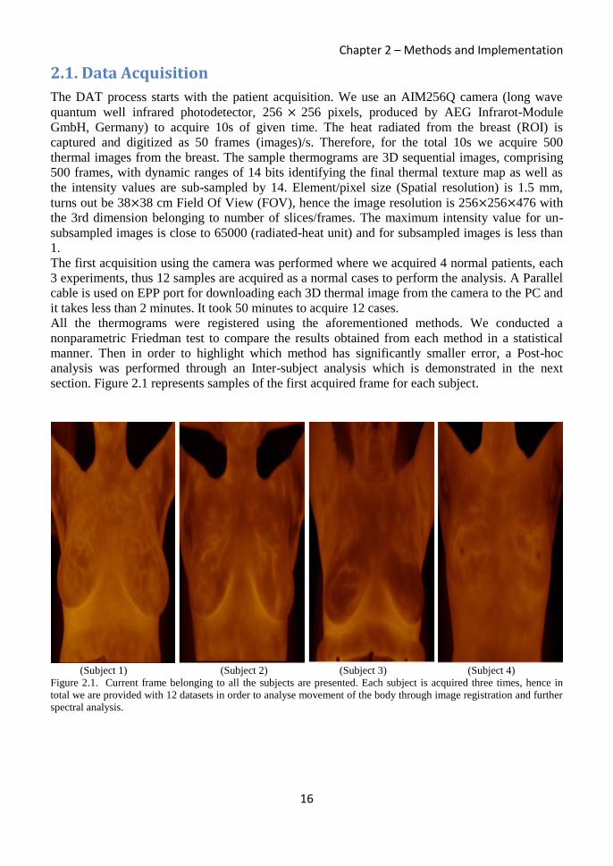
section. Figure 2.1 represents samples of the first acquired frame for each subject.
(Subject 1) (Subject 2) (Subject 3) (Subject 4)
Figure 2.1. Current frame belonging to all the subjects are presented. Each subject is acquired three times, hence in
total we are provided with 12 datasets in order to analyse movement of the body through image registration and further
spectral analysis.

Chapter 2 – Methods and Implementation
17
2.2. Breast Segmentation
After acquisition, in order to reduce the non-desirable artifacts, extra analysis and computational
time of the abovementioned algorithms, we segment the region of interest in the each frame of
the thermograms. Very few works have been done in this field due to a partially smoothed low
frequency components and high degree of noises and artifacts in the thermograms. In the
literatures, the thermograms are segmented first by an operator. Then breast quadrants are derived
automatically based on unique point of reference, i.e. the chin, the lowest, rightmost and leftmost
points of the breast. Recently few works addressing the automated segmentation have been
introduced where the identification of asymmetry by deploying Image Segmentation, Pattern
Recognition and Feature Extraction are considered as the basic methods to extract the region of
interest. There are several ways to performing the segmentation: “threshold-base”, “edge-base”
and “region base”.
The most cited work belongs to [26], which the idea is based on the fact that in a relatively
symmetric image, a small asymmetry could indicate a suspicious region. Hence, edge base
segmentation is performed by first Canny edge detection to identify the four dominant curves in
the edge image which is called “feature curves” including the left and right body boundaries and
the two lower boundaries of the breast. (Figure 2.2) Then the asymmetry analysis has been
performed by two methods of automated breast segmentation and tumor classification on the
images where we are interested in the former method in this phase. In this method simply using
the Hough transform the parabolic and the lower part of the breast is detected.
Figure 2.2. Thermal breast segmentation done using edge based method in [12].
There is another work having done by [23], which the use the same edge base semi-automated
segmentation while they consider more boundaries of the breast by taking into account the
detection of the region with highest curvature in the left and right body edges as well as
estimation of the top breast boundary using a number of empirical rules and body regions.
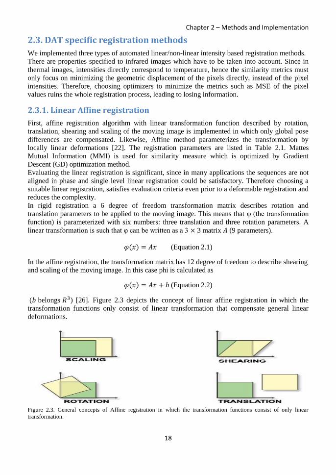
Chapter 2 – Methods and Implementation
18
2.3. DAT specific registration methods
We implemented three types of automated linear/non-linear intensity based registration methods.
There are properties specified to infrared images which have to be taken into account. Since in
thermal images, intensities directly correspond to temperature, hence the similarity metrics must
only focus on minimizing the geometric displacement of the pixels directly, instead of the pixel
intensities. Therefore, choosing optimizers to minimize the metrics such as MSE of the pixel
values ruins the whole registration process, leading to losing information.
2.3.1. Linear Affine registration
First, affine registration algorithm with linear transformation function described by rotation,
translation, shearing and scaling of the moving image is implemented in which only global pose
differences are compensated. Likewise, Affine method parameterizes the transformation by
locally linear deformations [22]. The registration parameters are listed in Table 2.1. Mattes
Mutual Information (MMI) is used for similarity measure which is optimized by Gradient
Descent (GD) optimization method.
Evaluating the linear registration is significant, since in many applications the sequences are not
aligned in phase and single level linear registration could be satisfactory. Therefore choosing a
suitable linear registration, satisfies evaluation criteria even prior to a deformable registration and
reduces the complexity.
In rigid registration a 6 degree of freedom transformation matrix describes rotation and
translation parameters to be applied to the moving image. This means that φ (the transformation
function) is parameterized with six numbers: three translation and three rotation parameters. A
linear transformation is such that φ can be written as a 3 × 3 matrix 𝐴 (9 parameters).
𝜑(𝑥) = 𝐴𝑥 (Equation 2.1)
In the affine registration, the transformation matrix has 12 degree of freedom to describe shearing
and scaling of the moving image. In this case phi is calculated as
𝜑(𝑥) = 𝐴𝑥 + 𝑏 (Equation 2.2)
(𝑏 belongs 𝑅3) [26]. Figure 2.3 depicts the concept of linear affine registration in which the
transformation functions only consist of linear transformation that compensate general linear
deformations.
Figure 2.3. General concepts of Affine registration in which the transformation functions consist of only linear
transformation.

Chapter 2 – Methods and Implementation
19
Likewise the previous algorithm, image moments are described as initialization. Evaluating the
linear registration along with the non-linear registration could be significant, since in many
applications the sequences are not aligned in phase and performing the single level linear
registration could be satisfactory in terms of final clinical evaluation. Therefore choosing the
most suitable linear registration for an application, might satisfy both technical and clinical
evaluation criteria even prior to applying a deformable registration and reduce the complexity and
computational time.
The transformation matrix has 12 degree of freedom to describe shearing and scaling. In order to
compute a reasonable value for the initial center of rotation and the translation, the initializer is
set to use the center of mass of each image as the initial correspondence correction. Centered
rigid with 6 degree of freedom transformation matrix describes rotation and translation
parameters. The CenteredRigid2DTransform supports two modes of operation. In the first mode,
the centers of the images are computed as space coordinates using the image origin, size and
spacing. The center of the fixed image is assigned as the rotational center of the transform while
the vector going from the fixed image center to the moving image center is passed as the initial
translation of the transform. In the second mode, the image centers are not computed
geometrically but by using the moments of the intensity gray levels. The center of mass of each
image is computed using the helper class ImageMomentsCalculator. The
CenteredRigid2DTransform is initialized by 5 parameters, indicating the angle of rotation, the
center coordinates and the translation to be applied after rotation. The initialization is done by the
CenteredTransformInitializer. The transform can operate in two modes, one assumes that the
anatomical objects to be registered are centered in their respective images. Hence the best initial
guess for the registration is the one that superimposes those two centers. This second approach
assumes that the moments of the anatomical objects are similar for both images and hence the
best initial guess for registration is to superimpose both mass centers.
2.3.2. Nonlinear parametric Bspline registration
Next, nonlinear parametric multi-level/multi-resolution Bspline method [23] is implemented and
applied. In a multi-level/multi-resolution registration, the idea is to first perform a linear
registration to roughly align the frames. Then we exploit the obtained transformation function
(bulk transformation) to characterize the further non-linear Bspline registration which consists of
coarse grid to cover the global anatomic deformations and fine grid resolution to compensate the
local motion with respect to number of Bspline grid points.
Categorizing the methods by the level/resolution of the registration, in a multi-level/multi-
resolution registration, the non-linear characterized Bspline registration is followed by the linear
registration in order to roughly align the frames, while the non-linear registration part is divided
to coarse and fine resolution with respect to number of bspline grid points. The multi-resolution
registration helps to localize the final alignment. Cost functions and registration parameters for
each method are presented in Table 2.1. For any point x,y,z part of the moving image the B-
Spline transformation is computed from the positions of the surrounding 4×4×4 control points.
𝑇(𝑥, 𝑦, 𝑧) = ∑ ∑ ∑ 𝐵𝑙(𝑢) + 𝐵𝑚(𝑣) + 𝐵𝑛(𝑤)𝐶𝑃𝑖+𝑙,𝑗+𝑚,𝑘+𝑛3𝑛=0
3𝑚=0
3𝑙=0 (Equation 2.3)
Where T is the transformation and i,j,k represents the index of the control point cell containing
the point (x,y,z) and u,v,w are the relative positions of point (x,y,z) inside that cell in the 3D
space. The control point at a specific location is represented by 𝐶𝑃𝑖+𝑙,𝑗+𝑚,𝑘+𝑛.
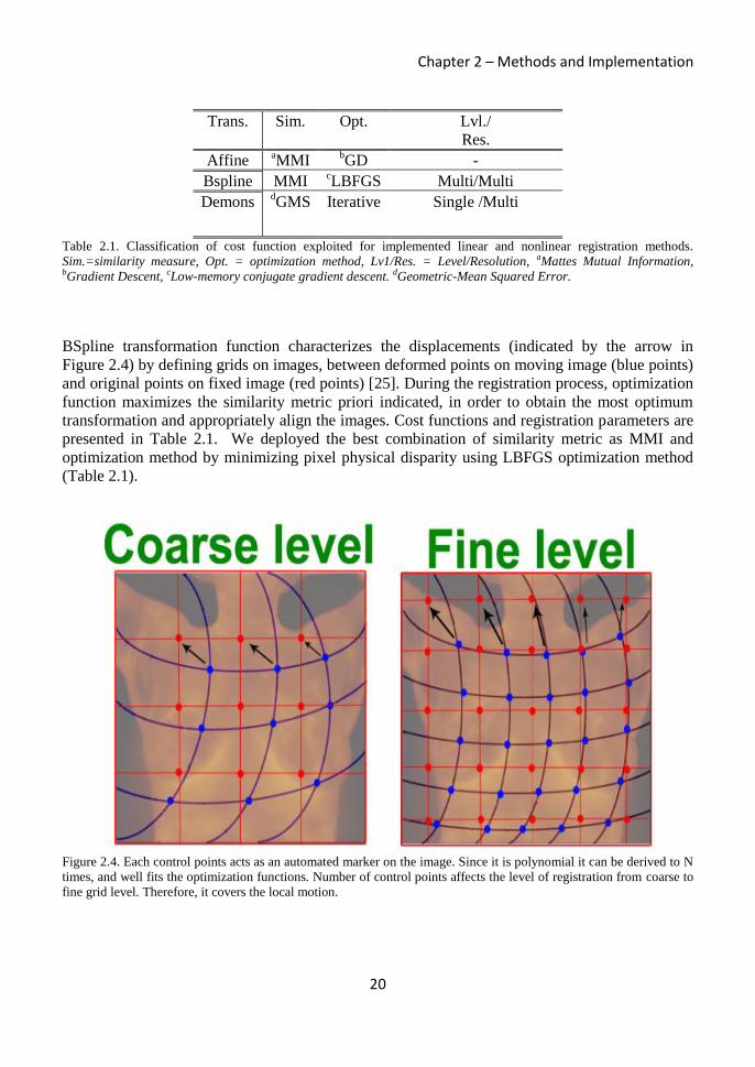
Chapter 2 – Methods and Implementation
20
Trans. Sim. Opt. Lvl./
Res.
Affine aMMI
bGD -
Bspline MMI cLBFGS Multi/Multi
Demons dGMS Iterative Single /Multi
Table 2.1. Classification of cost function exploited for implemented linear and nonlinear registration methods.
Sim.=similarity measure, Opt. = optimization method, Lv1/Res. = Level/Resolution, aMattes Mutual Information, bGradient Descent, cLow-memory conjugate gradient descent. dGeometric-Mean Squared Error.
BSpline transformation function characterizes the displacements (indicated by the arrow in
Figure 2.4) by defining grids on images, between deformed points on moving image (blue points)
and original points on fixed image (red points) [25]. During the registration process, optimization
function maximizes the similarity metric priori indicated, in order to obtain the most optimum
transformation and appropriately align the images. Cost functions and registration parameters are
presented in Table 2.1. We deployed the best combination of similarity metric as MMI and
optimization method by minimizing pixel physical disparity using LBFGS optimization method
(Table 2.1).
Figure 2.4. Each control points acts as an automated marker on the image. Since it is polynomial it can be derived to N
times, and well fits the optimization functions. Number of control points affects the level of registration from coarse to
fine grid level. Therefore, it covers the local motion.
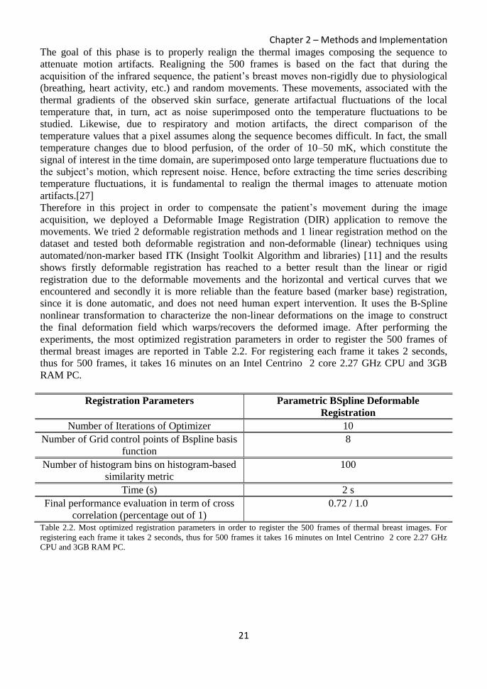
Chapter 2 – Methods and Implementation
21
The goal of this phase is to properly realign the thermal images composing the sequence to
attenuate motion artifacts. Realigning the 500 frames is based on the fact that during the
acquisition of the infrared sequence, the patient’s breast moves non-rigidly due to physiological
(breathing, heart activity, etc.) and random movements. These movements, associated with the
thermal gradients of the observed skin surface, generate artifactual fluctuations of the local
temperature that, in turn, act as noise superimposed onto the temperature fluctuations to be
studied. Likewise, due to respiratory and motion artifacts, the direct comparison of the
temperature values that a pixel assumes along the sequence becomes difficult. In fact, the small
temperature changes due to blood perfusion, of the order of 10–50 mK, which constitute the
signal of interest in the time domain, are superimposed onto large temperature fluctuations due to
the subject’s motion, which represent noise. Hence, before extracting the time series describing
temperature fluctuations, it is fundamental to realign the thermal images to attenuate motion
artifacts.[27]
Therefore in this project in order to compensate the patient’s movement during the image
acquisition, we deployed a Deformable Image Registration (DIR) application to remove the
movements. We tried 2 deformable registration methods and 1 linear registration method on the
dataset and tested both deformable registration and non-deformable (linear) techniques using
automated/non-marker based ITK (Insight Toolkit Algorithm and libraries) [11] and the results
shows firstly deformable registration has reached to a better result than the linear or rigid
registration due to the deformable movements and the horizontal and vertical curves that we
encountered and secondly it is more reliable than the feature based (marker base) registration,
since it is done automatic, and does not need human expert intervention. It uses the B-Spline
nonlinear transformation to characterize the non-linear deformations on the image to construct
the final deformation field which warps/recovers the deformed image. After performing the
experiments, the most optimized registration parameters in order to register the 500 frames of
thermal breast images are reported in Table 2.2. For registering each frame it takes 2 seconds,
thus for 500 frames, it takes 16 minutes on an Intel Centrino 2 core 2.27 GHz CPU and 3GB
RAM PC.
Registration Parameters Parametric BSpline Deformable
Registration
Number of Iterations of Optimizer 10
Number of Grid control points of Bspline basis
function
8
Number of histogram bins on histogram-based
similarity metric
100
Time (s) 2 s
Final performance evaluation in term of cross
correlation (percentage out of 1)
0.72 / 1.0
Table 2.2. Most optimized registration parameters in order to register the 500 frames of thermal breast images. For
registering each frame it takes 2 seconds, thus for 500 frames it takes 16 minutes on Intel Centrino 2 core 2.27 GHz
CPU and 3GB RAM PC.

Chapter 2 – Methods and Implementation
22
2.3.3. Symmetric diffeomorphic Demons registration
Finally symmetric diffeomorphic Demons registration method is implemented [28]. In the non-
parametric demons, by using gradient symmetric forces, the DF is obtained and it is warped onto
the moving image, by minimizing the following energy functional:
𝐸(𝑠, 𝑐) =1
𝛿𝑖2 𝑆𝑖𝑚(𝐹, 𝑀°𝑐) +
1
𝛿𝑥2 𝑑𝑖𝑠𝑡(𝑠, 𝑐)2 +
1
𝛿𝑇2 𝑅𝑒𝑔(𝑠) (Equation 2.4)
𝑆𝑖𝑚(𝐹, 𝑀°𝑐) represents geometric pixel disparity metric of fixed and moving image, 𝑑𝑖𝑠𝑡(𝑠, 𝑐)2
considers a correspondence error between transformation c and deformation field s as Gaussian
noise, hence as depicted in Figure 2.5 a Gaussian smooth kernel is applied on DF as a regularizer
along with smoothness degree of deformation 𝑅𝑒𝑔(𝑠) leading to well-posed framework as well
as a smoother vector field. 𝛿𝑖2, 𝛿𝑥
2, 𝛿𝑇2 maintain the trade-off between the three terms in the cost
function. Demons algorithm assumes pixels representing the same homologous point on an object
have the similar intensity on both the fixed and moving images, hence well suited for the time-
series thermogram registration. Significant parameters are listed in Table 2.3.
Figure 2.5. First, velocity field is obtained using gradient symmetric forces that is applied on the moving frames to
compensate the dissimilarities. Gaussian smooth kernel is deployed as additional regularizer. Fits for time-series
sequential thermal registration.
Label Iteration number Max step length Grid points number Reg. Time
(min)
Affine 200 0.1 - 45
Bspline a[20, 50] 10
b(15,30) 15
Demons 40 - - 15 Table 2.3. Registration parameters. Registrations are performed with Intel Core 2Duo 2.27 GHz CPU, 3GB RAM. a[linear level, non-linear level], b(coarse stage, fine stage).

Chapter 2 – Methods and Implementation
23
In the non-parametric demons, by using Symmetric Forces registration, the DF is obtained and it
is warped onto the moving image while match the histograms between source and target frames.
By exploiting multiple level pyramid registration approach, the registration process is fined and
localized. The demons algorithm relies on the assumption that pixels representing the same
homologous point on an object have the same intensity on both the fixed and moving images to
be registered, hence supposed to be well suited for the time-series sequential thermogram
registration. Therefore, number of bins where the histogram is matched could be considered as
the registration parameters.
2.4. DAT Registration evaluation methods
The fundamental issue for assessing the accuracy of registration relies on quantified comparison
of similarity between fixed and moving frames before registration and fixed and warped frames
after registration. We implemented three types of the most robust registration evaluation method
in order to both quantitatively and qualitatively evaluate the warped 3D thermograms.
2.4.1. DAT specific Breast Boundary Overlap
Aligning the boundaries of the breast correctly is one of the most fundamental expectations of the
breast thermogram registration. As a DAT specific evaluation method, “symmetric alignment of
breast boundaries assessment” of every frame is implemented in order to increase the accuracy
and the reliability of the evaluation.
Breast boundaries in all the frames are segmented using Canny Edge Detection and strong
gradient in every direction are obtained as a scalar value. Sum of squared differences of gradient
values are calculated between fixed frame and every warped frame after registration divided by
the number of voxels as breast boundary difference (Equation 2.5).
𝐵𝑜𝑢𝑛𝑑𝑎𝑟𝑦𝑑𝑖𝑓𝑓𝑒𝑟𝑒𝑛𝑐𝑒 =1
𝑛∑ (𝐼𝑓𝑏 − 𝐼𝑤𝑏)2
𝑖 𝑚
𝑖=2 (Equation 2.5)
Where 𝐼𝑓𝑏 and 𝐼𝑤𝑏 represent gradient values of breast boundary on fixed and warped images
respectively, 𝑖 is the frame number, m is the total number of frames and n is the number of voxels
in the images.
Then center of mass (C.O.M) of the image and both left and right breasts were determined.
Euclidean distances from C.O.M of the image to C.O.M of the left breast and to the right breast
were determined for fixed and every warped frame (see Figure 2.6). Eventually, as shown in
Equation 2.6, sum of squared error of the C.O.M distances between fixed and warped frames are
obtained as center-of-mass difference.
𝐶𝑂𝑀𝑑𝑖𝑠𝑡𝑎𝑛𝑐𝑒 =1
𝑛∑ [(𝐼𝑓𝑅 + 𝐼𝑓𝐿) − (𝐼𝑤𝑅 + 𝐼𝑤𝐿)]
2
𝑖 𝑚
𝑖=2 (Equation 2.6)
Above 𝐼𝑓𝑅 and 𝐼𝑓𝐿 represent Euclidean distance of right and left breast from the C.O.M of the
image respectively for the fixed frame and the same variables are defined for warped frames as
𝐼𝑤𝑅 𝑎𝑛𝑑 𝐼𝑤𝐿.
Finally as stated in the following equation, absolute difference of the two latter parameters
determined the measurement of breast boundary overlap (BBO) as which the final value should
be close to zero.
𝐵𝑟𝑒𝑎𝑠𝑡 𝐵𝑜𝑢𝑛𝑑𝑎𝑟𝑦 𝑂𝑣𝑒𝑟𝑙𝑎𝑝[𝐼, 𝑊] = |𝐶𝑂𝑀𝑑𝑖𝑠𝑡𝑎𝑛𝑐𝑒 − 𝐵𝑜𝑢𝑛𝑑𝑎𝑟𝑦𝑑𝑖𝑓𝑓𝑒𝑟𝑒𝑛𝑐𝑒| (Equation 2.7)

Chapter 2 – Methods and Implementation
24
Figure 2.6. A schematic view of how to obtain Breast Boundary Overlap as one of the DAT specific evaluation metrics
is depicted. C.O.M stands for centre of mass which are calculated for the whole image and each left and right breasts.
2.4.2. Normalized Mutual Information
Image difference residual is calculated via Normalized Mutual Information (NMI) to evaluate the
correspondence of fixed and all the moving frames for all the sequentially warped thermograms.
Using the {JoinImageFilter} we can obtain joint histogram of each image at first and then by
calculating the joint entropy among two images, the mutual information is obtained. By simply
adding entropies of each image and subtracting it from the joint entropy we can obtain mutual
information. [30]
Mutual Information = Entropy of image1 + Entropy of image2 – Joint Entropy
For evaluation of our second data type of clinical patients we use Normalized Mutual Information
(NMI), where the value of Mutual Information gets divided by the mean entropy of the input
images as follows:
Normalized Mutual Information =
2.0 * (Mutual Information) / ( Entropy of image1 + Entropy of image2 )
2.4.3. Jacobian determinant of the transformation
In order to analyze how physically logic the registration method is, an application to obtain
minimum Jacobian determinant of the transformation (Deformation Field) for each warped
frames of the sequences is implemented [31]. This metric investigates on the singularities of the
DF. If Jacobian value for each point is smaller than 1 local contraction has taken place and all the
points are singularities in the DF, indicating the irregularities in the transformation [32]. Hence,
the overall percentage of negative Jacobian values on all the sequential DF is obtained as a
quantitative evaluation metric. The Jacobian matrix is second order matrix of the deformation.

Chapter 2 – Methods and Implementation
25
𝐽𝜑(𝑥) =
𝜕𝜑1(𝑥)
𝜕𝑥1
𝜕𝜑1(𝑥)
𝜕𝑥2
𝜕𝜑1(𝑥)
𝜕𝑥3
𝜕𝜑2(𝑥)
𝜕𝑥1
𝜕𝜑2(𝑥)
𝜕𝑥2
𝜕𝜑2(𝑥)
𝜕𝑥3
𝜕𝜑3(𝑥)
𝜕𝑥1
𝜕𝜑3(𝑥)
𝜕𝑥2
𝜕𝜑3(𝑥)
𝜕𝑥3
The Jacobian matrix encodes the local stretching, shearing and rotating of the deformation field.
Useful measures that can be derived from the matrices are the determinants, which indicate
relative volumes before and after spatially transforming. A region of negative determinants would
indicate that the one-to-one mapping has been lost.
If 𝜑𝑐 is the deformation that results from the composition of two deformations 𝜑𝐵 and 𝜑𝐴 (i.e.
𝜑𝑐 = 𝜑𝐵. 𝜑𝐴 ), then the resulting Jacobian field can be obtained by the matrix multiplication
𝐽𝜑𝐶 = (𝐽𝜑𝐵. 𝜑𝐴) 𝐽𝜑𝐴. This leads to a similar scaling and squaring approach that can be used for
computing the Jacobian matrices of deformations.[33]
In practical approach we have written a program to evaluate the jacobian determinant of each
voxel of our final deformation fields using two following ITK filters.
itk::DisplacementFieldJacobianDeterminantFilter<DeformationFieldType, PixelType>
Computes a scalar image from a vector image (e.g., deformation field) input, where each output
scalar at each pixel is the Jacobian determinant of the vector field at that location. This
calculation is correct in the case where the vector image is a "displacement" from the current
location. The computation for the jacobian determinant is: det [𝑑𝑇
𝑑𝑥] = det [𝐼 +
𝑑𝑢
𝑑𝑥]. [33]
itk::MinimumMaximumImageCalculator<ImageType>
This calculator computes the minimum and the maximum intensity values of an image. It is
templated over input image type. To compute Maximum or Minimum value ComputeMaximum()
(ComputeMinimum()) functions can be called, otherwise Compute() will compute both. [33]
This application is based on [33] and it calculates the jacobian determinant of the first partial
derivative of the transformation. It computes the minimum and maximum jacobian value in the
whole vector field so that we can figure out whether we have any negative jacobian value for any
voxel or not. It also computes the percentage of voxels which its jacobian is less than 1, more
than 1 or equal to 1. It also gives us the final jacobian image applied on the vector field. (Figure
2.7)
In a Deformation Field, Jacobian values near 1 shows no local volume change in term of
quantification and in the jacobian image it is in grey, values lower than 1 show volume decrease
and are dark grey to black, and values above 1 (volume increase) are light grey to white. [33]
If we have the bigger percentage of jacobian values equal to 1 in any vector field, it might be
more consistent, non-singular and invertible. Also in term of minimum jacobian value in the
jacobian image, the positive and bigger number we have, the smoother deformation we will

Chapter 2 – Methods and Implementation
26
obtain. That is because we go far away from the zero and negative values. In contrast in term of
maximum jacobian value the smaller number we have the smoother vector field we will expect.
This application is very useful, since using this application, user can brightly obtain the ability of
the invertibility of its final deformation field and it shows to the user the potential of having
negative jacobian in the transformation which help for the final evaluation of the deformation
field.
Figure 2.7. Volume increase, decrease and no volume change after evaluating Jacobian determinant of the final
deformation. [33]

Chapter 3 – Results
27
Chapter 3 : Results
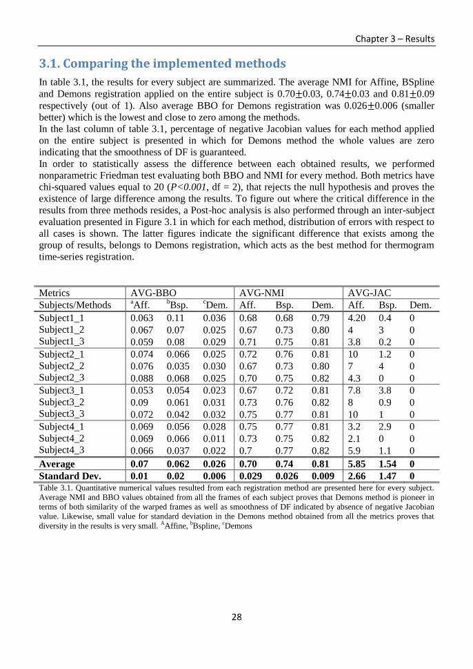
Chapter 3 – Results
28
3.1. Comparing the implemented methods
In table 3.1, the results for every subject are summarized. The average NMI for Affine, BSpline
and Demons registration applied on the entire subject is 0.70±0.03, 0.74±0.03 and 0.81±0.09
respectively (out of 1). Also average BBO for Demons registration was 0.026±0.006 (smaller
better) which is the lowest and close to zero among the methods.
In the last column of table 3.1, percentage of negative Jacobian values for each method applied
on the entire subject is presented in which for Demons method the whole values are zero
indicating that the smoothness of DF is guaranteed.
In order to statistically assess the difference between each obtained results, we performed
nonparametric Friedman test evaluating both BBO and NMI for every method. Both metrics have
chi-squared values equal to 20 (P<0.001, df = 2), that rejects the null hypothesis and proves the
existence of large difference among the results. To figure out where the critical difference in the
results from three methods resides, a Post-hoc analysis is also performed through an inter-subject
evaluation presented in Figure 3.1 in which for each method, distribution of errors with respect to
all cases is shown. The latter figures indicate the significant difference that exists among the
group of results, belongs to Demons registration, which acts as the best method for thermogram
time-series registration.
Metrics AVG-BBO AVG-NMI AVG-JAC
Subjects/Methods aAff.
bBsp.
cDem. Aff. Bsp. Dem. Aff. Bsp. Dem.
Subject1_1
Subject1_2
Subject1_3
0.063 0.11 0.036 0.68 0.68 0.79 4.20 0.4 0
0.067 0.07 0.025 0.67 0.73 0.80 4 3 0
0.059 0.08 0.029 0.71 0.75 0.81 3.8 0.2 0
Subject2_1
Subject2_2
Subject2_3
0.074 0.066 0.025 0.72 0.76 0.81 10 1.2 0
0.076 0.035 0.030 0.67 0.73 0.80 7 4 0
0.088 0.068 0.025 0.70 0.75 0.82 4.3 0 0
Subject3_1
Subject3_2
Subject3_3
0.053 0.054 0.023 0.67 0.72 0.81 7.8 3.8 0
0.09 0.061 0.031 0.73 0.76 0.82 8 0.9 0
0.072 0.042 0.032 0.75 0.77 0.81 10 1 0
Subject4_1
Subject4_2
Subject4_3
0.069 0.056 0.028 0.75 0.77 0.81 3.2 2.9 0
0.069 0.066 0.011 0.73 0.75 0.82 2.1 0 0
0.066 0.037 0.022 0.7 0.77 0.82 5.9 1.1 0
Average 0.07 0.062 0.026 0.70 0.74 0.81 5.85 1.54 0
Standard Dev. 0.01 0.02 0.006 0.029 0.026 0.009 2.66 1.47 0 Table 3.1. Quantitative numerical values resulted from each registration method are presented here for every subject.
Average NMI and BBO values obtained from all the frames of each subject proves that Demons method is pioneer in
terms of both similarity of the warped frames as well as smoothness of DF indicated by absence of negative Jacobian
value. Likewise, small value for standard deviation in the Demons method obtained from all the metrics proves that
diversity in the results is very small. AAffine, bBspline, cDemons

Chapter 3 – Results
29
Figure 3.1. In order to perform a Post-hoc analysis for nonparametric Friedman test (P<0.001, df = 2), box plots
representing distribution of errors on the obtained results from provided metrics for all the methods (inter-subject
evaluation) are presented. The analysis shows there is a critical difference in the groups of Demons method for every
experiment acting as the best method in our experiments.
Figure 3.2. Case variation error on all the methods performed on all the cases.
Based on breast boundary overlap error, we evaluate how well the dynamic frames of each case
within the subjects are aligned apart from the registration method. Hence the distribution of the
errors belonging to all the methods performed to each individual case is assessed, helping to
know which case has the least movement and better recovery. Figure 3.2 shows the error
distributed on each case.
0.01
0.02
0.03
0.04
0.05
0.06
0.07
0.08
0.09
0.1
Affine BSpline Demons
Inte
r-su
bje
ct B
BO
0.55
0.6
0.65
0.7
0.75
0.8
0.85
0.9
0.95
Affine BSpline DemonsIn
ter-
sub
ject
NM
I 0
1
2
3
4
5
6
7
8
9
10
Affine BSpline Demons
Ne
gati
ve J
aco
bia
n V
alu
es (
%)
0.01
0.02
0.03
0.04
0.05
0.06
0.07
0.08
0.09
0.1
Bre
ast
Bo
un
dar
y o
verl
ap E
rro
r (m
m, s
mal
ler
be
tte
r)
Case Variation evaluation
**
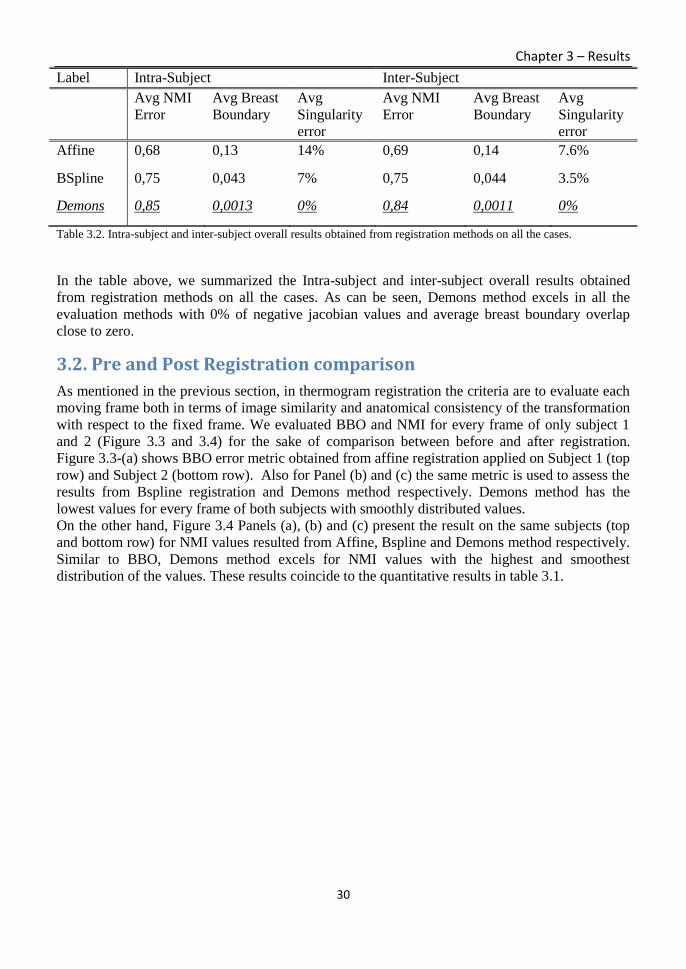
Chapter 3 – Results
30
Label Intra-Subject Inter-Subject
Avg NMI
Error
Avg Breast
Boundary
Avg
Singularity
error
Avg NMI
Error
Avg Breast
Boundary
Avg
Singularity
error
Affine 0,68 0,13 14% 0,69 0,14 7.6%
BSpline 0,75 0,043 7% 0,75 0,044 3.5%
Demons 0,85 0,0013 0% 0,84 0,0011 0%
Table 3.2. Intra-subject and inter-subject overall results obtained from registration methods on all the cases.
In the table above, we summarized the Intra-subject and inter-subject overall results obtained
from registration methods on all the cases. As can be seen, Demons method excels in all the
evaluation methods with 0% of negative jacobian values and average breast boundary overlap
close to zero.
3.2. Pre and Post Registration comparison
As mentioned in the previous section, in thermogram registration the criteria are to evaluate each
moving frame both in terms of image similarity and anatomical consistency of the transformation
with respect to the fixed frame. We evaluated BBO and NMI for every frame of only subject 1
and 2 (Figure 3.3 and 3.4) for the sake of comparison between before and after registration.
Figure 3.3-(a) shows BBO error metric obtained from affine registration applied on Subject 1 (top
row) and Subject 2 (bottom row). Also for Panel (b) and (c) the same metric is used to assess the
results from Bspline registration and Demons method respectively. Demons method has the
lowest values for every frame of both subjects with smoothly distributed values.
On the other hand, Figure 3.4 Panels (a), (b) and (c) present the result on the same subjects (top
and bottom row) for NMI values resulted from Affine, Bspline and Demons method respectively.
Similar to BBO, Demons method excels for NMI values with the highest and smoothest
distribution of the values. These results coincide to the quantitative results in table 3.1.

Chapter 3 – Results
31
(a) (b) ( c)
Figure 3.3. BBO metric is used to evaluate and compare each method applied before (blue line) and after (red line)
registration for every frame belonging to Subject 1 (top row) and Subject 2 (bottom row). X axis represents number of
frames from 1 to 476 and Y axis represents BBO error values (smaller better). Evaluated methods are presented as
Affine, Bspline and Demons respectively from left to right for panels (a), (b) and (c). Demons method shows the
lowest differences error for BBO comparing to other methods.
0
0.02
0.04
0.06
0.08
0.1
0.12
0.14
0.16
0.181
38 75
112
149
186
223
260
297
334
371
408
445
BB
O -
Su
bje
ct 1
(sm
alle
r b
ette
r)
Affine registration
0
0.02
0.04
0.06
0.08
0.1
0.12
0.14
0.16
0.18
1
35 69
103
137
171
205
239
273
307
341
375
409
443
Bspline registration
0
0.02
0.04
0.06
0.08
0.1
0.12
0.14
0.16
0.18
135 69
103
137
171
205
239
273
307
341
375
409
443
Demons registration
0
0.02
0.04
0.06
0.08
0.1
0.12
0.14
0.16
1
41 81
121
161
201
241
281
321
361
401
441
BB
O -
Su
bje
ct 2
(sm
alle
r b
ette
r)
0
0.02
0.04
0.06
0.08
0.1
0.12
0.14
0.16
1
38 75
112
149
186
223
260
297
334
371
408
445
0
0.02
0.04
0.06
0.08
0.1
0.12
0.14
0.16
1
35 69
103
137
171
205
239
273
307
341
375
409
443
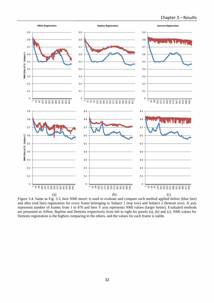
Chapter 3 – Results
32
(a) (b) (c)
Figure 3.4. Same as Fig. 3.3, here NMI metric is used to evaluate and compare each method applied before (blue line)
and after (red line) registration for every frame belonging to Subject 1 (top row) and Subject 2 (bottom row). X axis
represents number of frames from 1 to 476 and here Y axis represents NMI values (larger better). Evaluated methods
are presented as Affine, Bspline and Demons respectively from left to right for panels (a), (b) and (c). NMI values for
Demons registration is the highest comparing to the others, and the values for each frame is stable.
0
0.1
0.2
0.3
0.4
0.5
0.6
0.7
0.8
0.91
41 81
121
161
201
241
281
321
361
401
441
NM
I (O
ut
of
1) -
Su
bje
ct 1
Affine Registration
0
0.1
0.2
0.3
0.4
0.5
0.6
0.7
0.8
0.9
1
31 61 91
121
151
181
211
241
271
301
331
361
391
421
451
Bspline Registration
0
0.1
0.2
0.3
0.4
0.5
0.6
0.7
0.8
0.9
1
35 69
103
137
171
205
239
273
307
341
375
409
443
Demons Registration
0
0.1
0.2
0.3
0.4
0.5
0.6
0.7
0.8
0.9
135 69
103
137
171
205
239
273
307
341
375
409
443
NM
I (O
ut
of
1) -
Su
bje
ct 2
0
0.1
0.2
0.3
0.4
0.5
0.6
0.7
0.8
0.9
1
35 6910
313
717
120
523
927
3
307
341
375
409
443
0
0.1
0.2
0.3
0.4
0.5
0.6
0.7
0.8
0.9
133 65 97
129
161
193
225
257
289
321
353
385
417
449

Chapter 3 – Results
33
3.3. Spectral analysis of temperature modulation
The goal in this phase is to obtain final Power Spectral Density (PSD) image. Information on the
local blood perfusion is obtained from the spectral analysis of the time series at each image pixel.
In spectral analysis of thermograms, the range of frequency which is analyzed is between 0.1 Hz
and 1 Hz. The former 0.1 Hz frequency belongs to the vasomotor frequency, change in diameter
of the blood vessels caused by vasodilation and vasocontsrictions in the arteries and arterioles.
The latter frequency 1 Hz is the heart rate called cardiogenic frequency.[34] Those are in very
low-frequency range, shows the change in the temperature is very low and sudden change in
frequency must be captured during the frames. In order to obtain the final 2D PSD image, the
following sequential methods are applied on the registered thermograms:
1- First two pre-enhancement filtering are applied on each frame of the image: Median and
Average filtering in order to remove the noises and smooth the image while preserve the
high frequency components of the image.
2- For each pixel of each frame, we filter the signal using Yulewalk low pass Infinite
Impulse Response (IIR) filter with order of 15 and cut-off frequency at 10 Hz, (changes
the amplitude of each frequency components) removing mean value and make PSD
estimation using classic periodogram. We use sampling frequency of 50 Hz and 512
number of FFT points to calculate the PSD estimate. Likewise in order to preserve the
phase of the frequency components which changes the time order of the samples from
forward to backward, we use Zero-Phase filter to prevent the phase disorders.
3- Then we compute the FFT on the intensity/temperature-time series of the pixels to obtain
the fluctuation/changes in the temperatures and indicate the high/low frequency
components of the frames. Finally we estimate the PSD, out of computed FFT of every
corresponding pixels belonging to all the frames. In this part, we apply band on the
frequencies to which the PSD is computed. As mentioned the band is from 0.1 Hz to 4
Hz, which we consider the ambient noises as well. PSD can be computed as the Square
Magnitude of FFT scaled spectrum divided by the sampling period (Periodogram).
If we calculate PSD for every row of the frequencies, we obtain a PSD based 2D image
as shown in the last part.
After obtaining PSD image, there are several aspects/components/parameters regarding the
thermal spectral analysis of the obtained thermograms which could be analyzed and evaluated in
order to “detect” cancerous region/Tumor detection or to estimate the tumor contour from the
breast skin surface temperature or any other tumor parameters.
In the final PSD image, the difference of the suspicious region/lesion/cancer and the artifacts
cannot be well distinguished. Both belong to high frequency component of the image but in
different domain. The suspicious region belongs to high frequency, due to sudden change in the
temperature of the region and because of the vast frequent change in the temperature during the
acquisition time. Motion artifacts are then particularly relevant in areas in which a strong spatial
gradient of temperature is present. Distinguishing the latter two objects is considered as an issue.
Skin temperature fluctuations affect the signal of interest, thus applying registration on dynamic
thermogram images improves the spectral analysis of temperature modulation and reduces
percentage of false positive in the further diagnosis. PSD images are used for prognosis of breast
cancer in which the high frequency components of the temperature values are highlighted. We
obtained information on the local blood perfusion from the spectral analysis of the time series at

Chapter 3 – Results
34
each image pixel on Subject1-case1 by means of comparing the final spectral image with and
without applying registration as shown in Figure 3.5. The range of analyzed frequency is between
0.1 Hz (vasomotor frequency) and 1 Hz (cardiogenic frequency) [34]. High frequency
components of the image, where the power of the time-temperature signal is higher due to larger
temperature fluctuation, is highlighted by dark red (Figure 3.5-a). On the contrary, spots with
lower temperature modulation indicating smoother signal without unnecessary noises is shown in
lighter blue (Figure 3.5-b).
Followed by the PSD image, Time-temperature signal belonging to an arbitrary spot before and
after registration is also shown in Figure 3.6. Y axis represents temperature in the previous spot
which is equal to down quantized pixel intensity values.
Non-registered signal in the left panel shows a great variation in the temperature values ranging
from 0.6 to 0.7 during 10s acquisition, showing a huge fluctuation. However in the right panel
after registration, the vertical axis has been magnified in order to emphasis that the signal is quite
stabilized with a lower frequency and the intensities alter in a smaller scale between 0.61 and
0.62.
(a) (b)
Figure 3.5. Final 2D spectral image obtained from PSD values of each pixel without (a) and with (b) registration. High
frequency components of the temperature values for every pixel is shown as darker red and low frequency component
with lighter blue. Unnecessary noises are removed after registration (b), leading to a smoother image that helps in the
further diagnosis.

Chapter 3 – Results
35
(a) (b)
Figure 3.6. Time-temperature series of an arbitrary spot in Subject1-case1 belonging to before (a) and after (b)
registration. Acquisition time is 10s and vertical axis for panel (b) has been magnified in order to emphasis that the
scale of temperature variation is smaller after registration.
Figure 3.7. PSD-frequency graph of the latter time-temperature series for with (red) and without (blue) registration are
overlaid. As expected, frequency range is limited between 0.1 and 1 Hz and PSD values for the registered signal has
lower peak thus more stabilized comparing to non-registered curve.
Finally in Figure 3.7, PSD-Frequency curve of the latter time-temperature signal belonging to
before and after registration is overlaid for the sake of comparison. Peak of the PSD value for
registered signal is lower and smoother comparing to the nonregistered signal showing lower
power of the frequency component of the signal leading to stability and constancy in the
temperature oscillation during time variation.

Chapter 4 – Discussion and Conclusion
36
Chapter 4 : Discussion and Conclusion

Chapter 4 – Discussion and Conclusion
37
4.1. Discussion
The frequency of the any pixel (modulation change), could be staying static and we have the
phase shift or out of phase condition. Could be initial frequency angel of the sinusoidal wave and
we only have change in the angel. We have geometric changes, not change in the distance.
𝑥(𝑡) = 𝐴. cos (2𝜋𝑓𝑡 + 𝜑) (Equation 4.1)
𝑦(𝑡) = 𝐴. sin(2𝜋𝑓𝑡 + 𝜑) = 𝐴. cos (2𝜋𝑓𝑡 + 𝜑 − 𝜋2⁄ ) (Equation 4.2)
Considering the temperature in a point at a given time, total derivative of temperature with
respect to time is proportional to velocity of skin portion, hence Demons method, calculates the
2D velocity in the image, approximating image motion from sequential time-ordered images,
which also guarantees the similarity of warped frames.
Demons method computes a deformable registration based on intensity changes and is derived
from the work by Thirion10. The registration is driven by the concept of optical flow and was
initially used in computer vision research. Optical flow calculates an image velocity
approximating image motion from sequential time-ordered images. The demons algorithm is
based on gradient calculations from the fixed image to determine the demons force required to
deform the moving image. The diffusion model assumes that so-called “demons” at every voxel
from the fixed (reference) image are applying forces that push the voxels of the moving image
into matching up with the fixed image.
The inputs to the registration are a moving image m and a fixed image f. We assume that f and m
are consecutive “snapshots" of an image function I(x,y,z,t) for which the brightness values of
corresponding anatomy are constant. Explicitly including time as a variable gives
I(x(t),y(t),z(t), t) = constant
and f = I(x(t0),y(t0), z(t0), t0), m = I(x(t1),y(t1), z(t1),t1). The optical flow velocity can then be
written as
�⃗� = (𝑚−𝑓)∇⃗⃗⃗𝑓
|∇⃗⃗⃗𝑓|2
+𝐾2(𝑚−𝑓)2 (Equation 4.3)
In optical flow, v is considered to be a velocity because the images are two successive time
frames; v is the displacement during the time interval between the two image frames. f ∇r
represents the relationship between the neighboring points in the fixed image (such as an edge),
K is the reciprocal of the diagonal of a pixel (units of 1/mm) and the (m-f) term represents the
differential force of the interaction between the fixed and the moving images.
Equation (4.3) is calculated iteratively; after each iteration, the optical flow computation is
followed by regularization of the deformation field using a Gaussian filter.
In order to qualitatively evaluate the methods, Figure 4.1 illustrates the sequential final DF
obtained for Subject1-case1 overlaid on the warped frames. Comparing the DF in each method,
vectors in affine registration shows a disordered and irregular pattern conveying misalignment
and failure in compensating the physical distance of corresponding points. Likewise, movements
of the lower part of the body have not been compensated and remain in the same structure.

Chapter 4 – Discussion and Conclusion
38
(Affine) (Bspline) (Demons)
Figure 4.1. DF overlaid on warped images belonging to current frame of Subject1-case1, in order to show the
smoothness of final DF yielded for each method. Demons resulted with the least irregularity in DF along with the
shortest vectors of displacements proving that misalignment of the warped frames is well compensated.
This is because nonlinear deformation of the body movement is neglected and transformation
mapping of two images only contains straight lines and points leading to compensation of only
rigid body motion.
However in Figure 4.1, vectors in Bspline registration have covered movements in every part of
the body, although there are unorganized directions as well as large magnitudes of the vectors
due to the fact that image similarity function does not uniquely determine the correspondence
between two image volumes. Here despite of developing multi level/resolution registration to
keep the localization during the process, however similarity cost functions have many local
minima due to the complexity of the images being matched and the dimensionality of the
transformation [22]. The latter issue leads to uncertainty in the physiological consistency of
deformation between two images. The problem is usually resolved by including a regularization
function into the cost function in order to reduce the irregularities in the deformation field.
Demons registration has resolved both latter problems and yielded smaller BBO error and higher
NMI values (Figure 3.4). Basically in Demons algorithm, histogram matching is very crucial
since we could have different scales of gray levels between the reference frame as the very first
frame and the further frames with large movements. Hence, it assumes that the corresponding
points on both images remain the same intensity value which acts significant in application of
DAT breast cancer detection where temperature parameters play the main role.
DF in the Demons method is the smoothest comparing to other methods, due to the fact that
considering the temperature in a point at a given time, total derivative of temperature with respect
to time is proportional to velocity of skin portion [22]. Demons method, calculates the 2D
velocity in the image, approximating image motion from sequential time-ordered images, which
also guarantees the similarity of warped frames. Moreover, it computes optical flow at every
pixel and assumes motion displacement but no intensity error, and uses Gaussian kernel to
smooth the deformation field after each iteration.
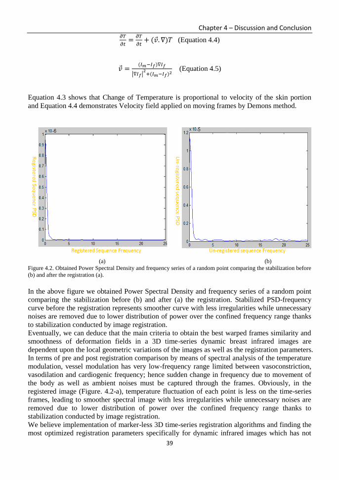
Chapter 4 – Discussion and Conclusion
39
𝜕𝑇
𝜕𝑡=
𝜕𝑇
𝜕𝑡+ (�⃗�. ∇)𝑇 (Equation 4.4)
�⃗� =(𝐼𝑚−𝐼𝑓)∇𝐼𝑓
|∇𝐼𝑓|2
+(𝐼𝑚−𝐼𝑓)2 (Equation 4.5)
Equation 4.3 shows that Change of Temperature is proportional to velocity of the skin portion
and Equation 4.4 demonstrates Velocity field applied on moving frames by Demons method.
(a) (b)
Figure 4.2. Obtained Power Spectral Density and frequency series of a random point comparing the stabilization before
(b) and after the registration (a).
In the above figure we obtained Power Spectral Density and frequency series of a random point
comparing the stabilization before (b) and after (a) the registration. Stabilized PSD-frequency
curve before the registration represents smoother curve with less irregularities while unnecessary
noises are removed due to lower distribution of power over the confined frequency range thanks
to stabilization conducted by image registration.
Eventually, we can deduce that the main criteria to obtain the best warped frames similarity and
smoothness of deformation fields in a 3D time-series dynamic breast infrared images are
dependent upon the local geometric variations of the images as well as the registration parameters.
In terms of pre and post registration comparison by means of spectral analysis of the temperature
modulation, vessel modulation has very low-frequency range limited between vasoconstriction,
vasodilation and cardiogenic frequency; hence sudden change in frequency due to movement of
the body as well as ambient noises must be captured through the frames. Obviously, in the
registered image (Figure. 4.2-a), temperature fluctuation of each point is less on the time-series
frames, leading to smoother spectral image with less irregularities while unnecessary noises are
removed due to lower distribution of power over the confined frequency range thanks to
stabilization conducted by image registration.
We believe implementation of marker-less 3D time-series registration algorithms and finding the
most optimized registration parameters specifically for dynamic infrared images which has not
Chapter 4 – Discussion and Conclusion
40
been done before can ease the patient acquisition procedure by making it user-independently and
compensate the patient movement as well as ambient noises; thus clearer time-temperature signal
of interest can be transformed for the advance spectral analysis of temperature modulation for the
following breast cancer prognosis. It is expected that registration strategy and its characteristics
introduced in this paper, plus the obtained results may be used in future design optimization of
many DAT framework and DIRI applications.
However there are some limitations on the implementation and deployment of the algorithms.
The major problem resides on the complexity of the methods in terms of implementation.
Considering each method, large numbers of parameters are involved e.g. number of histogram
bins of MI as similarity metrics, max/min step length of the optimization functions and cost
function convergence tolerance. This issue makes the procedure nontrivial. Likewise, there is a
computational burden during the deployment of the implemented methods, thus in some points a
parameter tuning is required in order to reduce the calculation cost. For this purpose porting the
implementation from CPU to GPU enabled environment can advance computational pace.
4.2. Conclusion
Respiratory motion can be a significant effect when applying breast infrared thermography.
Manual marker-based registration methods have been used in the previous works to resolve the
patient movement along with ambient noises during the thermogram acquisition, but there are
drawbacks e.g. difficulty in manually placing the markers, optimal number of markers
obstructing the acquisition procedure. Likewise, unnecessary noises in the time-temperature
signals lead to inaccurate further spectral analysis of the temperature modulation.
We implemented time-series image registration techniques in ITK, comprising linear affine and
nonlinear Bspline as well as Demons registration method. The methods are both quantitatively
and qualitatively validated by robust evaluation metrics, i.e. Normalized Mutual Information,
Breast Boundary Overlap and Jacobian determinant of the transformation. Spectral analysis is
also performed to compare the signals of time-temperature series on each pixel before and after
registration. Based on the results along with nonparametric Friedman test and the further Post-
hoc analysis, we deduced that Demons registration due to homologous symmetric forces
enforcing the pixel geometric disparities to be shortened on all the frames, excelled in terms of
both frame similarity and smooth DF, comparing to other methods. Likewise, registered spectral
image was smoother because of stabilized noiseless low frequency components of each pixel that
helps in the further prognosis of breast cancer.
Finally, obtaining optimal DAT registration parameters is considered as a future work.

41
THIS PAGE WAS INTENTIONALLY LEFT BLANK

42
Section 2: Preoperative Computer Aided Diagnostic System for Carotid Artery Stenting simulation using Finite Element Analysis

Chapter 5 – Introduction to Arterial Stenting
43
Chapter 5 : Introduction to Carotid Arterial Stenting

Chapter 5 – Introduction to Arterial Stenting
44
5.1. Calcified carotid atherosclerotic plaque and Agatston score
Understanding mechanical and material behavior of arteriosclerotic cardiovascular disease in
terms of both atherogenesis and thrombogenesis that lead to ischemic stroke has been in debate.
Carotid artery stenting (CAS) of cervical carotid artery stenosis has been increasingly used as an
alternative to carotid endarterectomy (CEA). Realizing mechanism of plaque rupture inside
intracranial carotid artery in order to predict the pre-operative interaction of plaque/stent/balloon
and the arterial wall in an interventional treatment of CAS operation could prevent a high risk of
stroke. Histology of atherosclerosis plaques in an advanced stage consist of different layers:
fibrous cap, fibrotic intima, calcification, lipid pool and fibrotic media [35], [36]. In this work we
specifically focused on carotid calcified plaques extracted from MDCT angiography. Although it
has been suggested that calcifications stabilize the plaque fibrous and prevent the rupture [37],
however when becomes larger and advanced, it causes plaque break [38]. Presence of
calcification inside the fibrous cap indicates a hard and concentric plaque in which alters the
mechanical properties of the plaque [39], [40]. Likewise there is a direct relationship between
percent area of calcification and volume of plaque thus severity of occlusion [41].Two major
problems exist in CAS angioplasty: (i)elastic and small plaques with early calcifications
penetrate into the stent leading to “plaque protrusion”. (ii)stiff and large caps which contain
advanced calcifications when being pushed by the stent/balloon lead to eventual arterial wall
rupture or stent fracture during the operation. Investigation on clinical as well as mechanical
behavior of fibrous cap, lipid pools and different arterial layers have been extensively performed
[42], [43], however there is lack of probe into association of calcification and physiological
phenomena that occurs during the development of atherosclerosis as well as susceptibility of the
carotid plaque during CAS angioplasty. The aim of this work is to particularly explore on
contribution of calcification in atherosclerotic plaque rupture and to find its maximum resistance
when imposed by external pressure load during interventional CAS placement by exploiting
Agatston Calcium score.
Figure 5.1. Schematic representation of an elastic artery. Adapted from Rhodin [9].

Chapter 5 – Introduction to Arterial Stenting
45
As illustrated in Figure 5.1, all blood vessels share some common characteristics, for example,
they consist of three distinct layers or tunicae: The tunica intima, tunica media and tunica
adventitia. In young human arteries the intima is a thin endothelial layer that lines the inside
walls, and sits on a very thin (∼80 nm) basal lamina of a net-like type IV collagen. In general, the
endothelial cells tend to be elongated in the direction of the blood flow. They act as a
semipermeable membrane, through which nutrients and chemical signals can reach the cells in
the vessel wall from the bloodstream. The intima has also a key role in regulating the active
response of the vessel: as a membrane, it is the conduit through which pressure regulating agents
reach the media. Additionally, it is known that the intima produces NO (nitric oxide), which
relaxes smooth muscle cells in the media and thus helps control the vascular tone. Despite its
great functional importance, due to its small thickness in young arteries the intima is usually
neglected when considering the different layer contributions to the global mechanical resistance
of the vessel wall. The intima is separated from the media by the internal elastica lamina, a
fenestrated sheet of elastin. The media is formed primarily by smooth muscle cells (SMC) that
are embedded in an extracellular plexus of elastin and collagen (mainly types I and III) and an
aqueous ground substance that also contains proteoglycans. Depending on the internal
arrangement of the smooth muscle cells in the media, it is distinguished between elastic arteries
and muscular arteries. The former tend to be large-diameter vessels close to the heart, and
include the aorta, the main pulmonary artery, the common carotid and common iliac arteries.
Their most characteristic histological feature is the so-called lamellar unit, a sandwich-like
‘sublayer’ of smooth muscle cells and thin elastic laminae. Histological sections of elastic arteries
show concentric ring-like structures (Fig. 5.1), as many as 40 to 70 in thick vessels like in the
human aorta, that are tied together by radially oriented collagen. In muscular arteries, the media
appears as a single thick ring of smooth muscle cells. The SMC are embedded in a loose
connective tissue matrix and arranged as a sequence of concentric layers of cells, which can reach
numbers of 25-40 in larger vessels like in the femoral artery. Sometimes it is difficult to identify
clearly between elastic and muscular arteries, due to the fact that abrupt changes do not occur in
continuous structures like the vasculature. These transitions occur smoothly and the
corresponding artery segments loose their characteristical lamellar structure progressively, as
happens in the internal and external carotid arteries. Finally, the adventitia is the outermost layer
of the vessel wall. It consists of a dense network of type I collagen fibers with scattered
fibroblasts, elastin and nerves.

Chapter 5 – Introduction to Arterial Stenting
46
Figure 5.2. Many parts and sections of carotid arteries, in addition to plaque build-up progression inside the artery.
Figure 5.2, illustrates the build-up of plaque in the internal carotid artery may lead to narrowing
and irregularity of the artery's lumen, preventing proper blood flow to the brain. More commonly,
as the narrowing worsens, pieces of plaque in the internal carotid artery can break free, travel to
the brain and block blood vessels that supply blood to the brain. This leads to stroke, with
possible paralysis or other deficits.
Atherosclerosis is a local inflammatory disease of the arteries that primarily alters the conduit
function by reducing the lumen, sometimes completely blocking blood flow. Atherosclerosis
appears preferably at junctions and branches of conduit arteries (like coronary arteries and carotid
bifurcation), always at sites of altered flow patterns. (Figure 5.3)
Figure 5.3. Progression of atherosclerotic disease. From the initial state, where LDL migrate through the endothelium
in the intima (left side) to the beginning of intima thickening (right side). Illustration adapted from [44].

Chapter 5 – Introduction to Arterial Stenting
47
The natural history of atherosclerosis starts with the formation of fatty streaks by a specific
trapping and retention of lipoproteins at lesion prone sites, due to an imbalance between the LDL
(low density lipoprotein) concentration in the tissue with respect to the plasma. When this
happens, the lipids are trapped in the extracellular matrix, in the basal zone of the intima. If this
trapping is pathologic, there is an increase of leukocytes that adhere to the endothelial surface,
supported by the expression of specific adhesion molecules. This is seen as the start of the
inflammatory response. As a result, monocytes enter the artery wall and rapidly differentiate into
tissue macrophages, subsequently transforming into foam cells by ingesting trapped and modified
lipoproteins. Many of the foam cells within the lesion become activated to express a large
number of additional factors that likely play important roles in the atherogenic process, from
inducing anomalous behavior of healthy cells to providing a favorable biochemical environment
for disease progression (Figure 5.3).
A more advanced lesion is hallmarked by the formation of a fibrous cap [44, 45]. In this process,
smooth muscle cells migrate from the media to the intima and change phenotype, switching from
being contractile to a cell type which proliferates and produces large amounts of connective
tissues [46]. The fibrous cap acts as a protective shield for the underlying lipid pool, which has a
necrotic core with interspersed microscopic calcium nodules. At this stage, there is a significant
dysregulation of the vascular tone, likely due to a reduction in NO availability to the now
atrophic media.
In the final stage, the atheromatous plaque described above may either become stable, in which
case it only impairs blood flow, or unstable, where it is at risk of rupturing and developing its
highly thrombogenic contents into the blood stream. It has been established that it is the plaque
composition, rather than its size, that determines its instability [47, 48].
From this short description, it is obvious that the structure and the mechanics of the wall changes
dramatically in the event of atherosclerosis.

Chapter 5 – Introduction to Arterial Stenting
48
Figure 5.4. Calculation of plaque volume in a step-by-step fashion using the software and measurement of percent
stenosis is demonstrated. (a) Manually drawn region of interest for sculpting is depicted on the coronal maximum
intensity projection (MIP) image. (b) Calcified plaque on the sculpted MIP. (c) Volume rendered appearance of the
plaque with automatic calculation of calcified plaque volume with a single button click, calculated to be 0.25cm3 in this
patient. (d) Calculation of percent stenosis on lateral view of carotid digital subtraction angiography.
In figure 5.4, we depicted calculation of plaque volume in a step-by-step fashion using the
software and measurement of percent stenosis is demonstrated. (a) Manually drawn region of
interest for sculpting is depicted on the coronal maximum intensity projection (MIP) image. (b)
Calcified plaque on the sculpted MIP. (c) Volume rendered appearance of the plaque with
automatic calculation of calcified plaque volume with a single button click, calculated to be
0.25cm3 in this patient. (d) Calculation of percent stenosis on lateral view of carotid digital
subtraction angiography. The luminal diameter was measured at the narrowest part (A), which
was a post-bulbar location for this particular case; B corresponds to the luminal diameter in the
distal cervical internal carotid artery with percent stenosis and was calculated using the following
formula: Percent stenosis 5(B–A)/B, yielding a 55% stenosis for this patient.

Chapter 5 – Introduction to Arterial Stenting
49
The Agatston score is the EBCT-based scale used to quantify coronary calcification and has
plentiful data to support its usefulness. It is based on the density measurements of the calcium.
The Agatston score is reproducible to 15%–20%. The reason the Agatston score is accurate only
to 15%–20% is that the density of the calcium is assigned a weighting factor (density score) in a
stepwise manner that is not linear or continuous. As illustrated in Figure 5.5, an insignificantly
different Hounsfield unit score could yield a significantly different density score. Because the
Agatston score is a product of this density factor and the area of the calcium in the artery, a
density score that is a factor higher will yield an Agatston score that is an order of magnitude
different despite the fact that the Hounsfield unit scores for the calcium were very similar. For
example, a Hounsfield unit score of 200 will result in a density factor of 1, whereas a score of
201 will yield a density score of 2. If the calcified area is 5 pixels, then the Hounsfi eld unit score
of 200 will yield an Agatston score of 5 (product of a density score of 1 and a calcium area of 5
pixels). The Hounsfield unit score of 201 (not significantly different from a score of 200 as in the
above example) will yield an Agatston score of 10 (product of a density score of 2 and a calcium
area of 5 pixels) because the density factor was stepped up to 2 (Figure 5.5).
If we assume the area of the calcified plaque=4mm2 and Peak HU=270 the based on above
equation Ca score for one slice = 8. Continuously, If slice thickness is 1 mm and number of slices
over volume=220 the whole Ca Score of the plaque would be 220x8=1760.
Figure 5.5. Stepwise relationship between Hounsfield units and the calcium density score as they relate to the
determination of the Agatston score.
In the literature, [49] performed an elaborated study on preoperative simulation of CAS using
Finite Element Method (FEM), by choosing single image based data to model the stent, vessel
and the plaque. Two homogenous and non-homogenous material properties are defined based on
constitutive law strain energy function and maximum stress obtained from each material
properties are reported as 152 KPa and 91.3 KPa respectively. However plaque is considered as
one body with no classification of different fibroatheroma layers and nonlinearity of
atherosclerosis material characteristics are not fully perceivable. Chau et al. [42] investigated on
post-expansion response of the slotted tube in the presence of plaque and artery. The
configuration is not extracted from a patient-specific framework, thus it is a virtual design of the

Chapter 5 – Introduction to Arterial Stenting
50
CAS simulation. Material properties for plaque and artery are defined as linear isotropic. The
maximum pressure load on plaque was specified as 2.65 MPa with max Von mises stress of
plaque equal to 0.883 MPa. Wong et al. [43] performed an elaborated study on anisotropic and
elastic mechanical impact of carotid calcified plaque in rupture using single model geometry by
exploiting two dimensional structural analyses. Virtual simulation showed critical stress is lower
for calcified plaques than that of non-calcified one emphasizing the stabilization of fibroatheroma
plaque. Zhao et al. [44] conducted a single computational model of Finite Element Analysis
(FEA) to simulate CAS procedure and compare the ultimate mechanical properties of soft and
calcified plaque. Smaller stress distribution was reported in calcified plaque with respect to soft
plaque due to energy absorption by calcification indicating the less arterial vulnerability. Another
statistical study was performed by Yang et al. [45] that investigated on association of mechanical
properties of carotid calcified plaque progression measured by wall thickness increase (WTI) on
in vivo Magnetic Resonance Imaging (MRI) data. They found a negative linear correlation
between WTI and plaque wall stress confirming that increase in plaque size leads to lower flow
wall shear stress. They also performed linear regression analysis for predicting a patient-specific
quantitative plaque growth functions.
5.2. Carotid Artery Stenting
In order to perform CAS, a small incision is made in the patient’s groin, arm or wrist. A catheter
is introduced into an artery in the body through this incision, and the physician advances it to the
narrowed part of your carotid artery. Next, a special filter is delivered through the catheter and
placed just beyond the narrowed section of the artery. This small filter is part of a system
(embolic protection system) designed to catch and remove plaque and other particles that may be
released during the procedure. After the embolic protection device is in place, the artery may
need to be enlarged to make room for the stent. To do this, the physician places a small, deflated
balloon through the catheter to the blocked area of the carotid artery. When the balloon is in the
right place, it is inflated. This pushes the plaque buildup aside and reopens the artery to restore
blood flow. The balloon is deflated and removed. Then a small metal mesh tube called a stent is
placed in the artery and is expanded to prop the artery open and allow blood flow to the brain
(Figure 5.6). After the stent is implanted, a balloon may be inflated inside the stent to better
position the stent against the artery wall; then the balloon, filter and catheter are removed. The
incision in the groin, arm or wrist is closed. The stent remains in place to help prevent future
narrowing of the carotid artery.

Chapter 5 – Introduction to Arterial Stenting
51
Figure 5.6. Real size and shape of an angioplasty stent that is a small tube mesh.
The abovementioned procedure has been illustrated in the figure 5.7 (b) below by using a closed-
cell stent. Panel (a) in Figure 5.7 depicts the angioplasty balloon expanded by the catheter inside
the artery in order to press the atherosclerotic plaque.
(a) (b) Figure 5.7. (a)Angioplasty balloon inserted by the catheter is depicted inside the artery to push the plaque. (b) the
whole procedure of carotid artery stenting is illustrated by a closed-cell stent.

Chapter 5 – Introduction to Arterial Stenting
52
5.3. Material and Mechanical parameters
First we have to prove how Ca score is related to hardness of the calcified plaque. We have to
find a correlation between the Ca score, stiffness and hardness. Stiffness means elasticity and
hardness means plasticity. Stiffness measures how linearly the stress that imposed on the plaque
responds as strain and it elongates from the initial length. Stiffness is shown as young’s modulus
and it only depicts the elasticity of the plaque below the Yield strength. Hence the slope of the
stress-strain curve represents young’s modulus.
If one object goes beyond the yield strength without rupture then it has non-linear material model
which is called plasticity. In the stress-strain curve after the yield point, the slope of the curve
represents how plastic is the object and it is measured using Tangent modulus. The curve
continues until reaches to Ultimate tensile strength which beyond that point the object ruptures or
breaks (Figure 5.8).
Figure 5.8. A general stress-strain curve that demonstrates elastic and plastic/linear and nonlinear domains of a
parameter.
Since biomaterial objects such as tissues are non-linear materials, so we consider them having
plasticity in behavior. Elasticity for the material is defined by young’s modulus and Poisson ratio
where plasticity is defined by yield strength and tangent modulus as mechanical parameters. We
consider biomaterials as non-homogenous but isotropic in our analysis. Isotropic means the
direction of the loads imposed on the plaques is not considered in our analysis and they all have
isotropic and ubiquitous responds to the loads. Non-homogenous means we consider the calcified
plaques composed as different composition, not one material, hence we define different density
for each calcified plaque. Therefore in order to analyze hardness of the plaque, we must consider
both its Elasticity and Plasticity. In Figure 5.9, the main concepts for Elastic modulus and
evaluation of compressibility as Poisson’s ratio have been depicted.

Chapter 5 – Introduction to Arterial Stenting
53
(a) (b)
Figure 5.9. (a) Depicts the main principle of Young’s modulus (Elastic modulus) and (b) Poisson’s ratio.
In the following equations the main equations in order to obtain the Young’s modulus of
elasticity (Elastic Modulus) and Poisson’s ratio of compressity have been shown.
𝑌𝑜𝑢𝑛𝑔′𝑠 𝑀𝑜𝑑𝑢𝑙𝑢𝑠 = 𝐸𝑙𝑎𝑠𝑡𝑖𝑐 𝑀𝑜𝑑𝑢𝑙𝑢𝑠 = 𝐸 =𝑠𝑡𝑟𝑒𝑠𝑠
𝑠𝑡𝑟𝑎𝑖𝑛=
𝐹𝐴⁄
∆𝐿𝐿⁄ (Equation 5.1)
𝑃𝑜𝑖𝑠𝑠𝑜𝑛′𝑠 𝑟𝑎𝑡𝑖𝑜 = (𝑤−𝑤0) 𝑤⁄
(𝐿−𝐿0)𝐿⁄
(Equation 5.2)
5.3.1. Volume score
Ca score is composed of three elements. HU, Area and Volume. Based on the fact that no
significant correlation exists between percent area of calcification and the maximum stress thus
stiffness [54], hence the element of volume and area do not influence hardness of the calcium.
Also it has been suggested that it is the type of the calcification that leads to plaque rupture not
the size [55]. Therefore, we conclude largeness of the plaque has no impression on the plaque
rupture and its hardness.
5.3.2. Elasticity
It has been suggested that existence of the calcification leads to stiffness of the arterial wall, thus
the aortic calcification is associated with aortic stiffness [54], [55]. It means high Ca Score must
lead to higher stiffness, which means elasticity of the plaque changes with different Ca score. We
have to assign different Young’s modulus to each plaque. Therefore, we can say there is a linear
and positive proportion between Ca score and stiffness. Ca score is associated with stiffness.
Afterwards, we focus on the last element HU. We have to prove that higher HU means higher
stiffness. There is not such equation relationship which states higher HU leads to higher stiffness
specially in biomaterials because of their non-linearity in material behavior, but based on [57] we
can statistically prove that higher HU leads to stiffer material in terms of young’s modulus. In
[57] Cortical bone and Cancellous bone (Spongy bone) are analyzed in order to relate HU,
Density and young’s modulus using linear and exponential regression empirically.
First, we used the method in [58] to obtain density of the calcified plaque base on its HU using
the related and appropriate equations. Then we obtain the young’s modulus using the density that

Chapter 5 – Introduction to Arterial Stenting
54
was obtained above via following equations to correlate the HU, density and young’s modulus for
each plaque [57]. I considered the cortical bone as the main tissue that form the bones, therefore
it is dense and stiff which release chemical materials mainly Calcium. Spongy bone is less dense
and soft and it combines with cortical bone to form the whole skeleton. The correlation range of
HU and bone types is presented in the following chart [57].
a) Compactcorticalbone→≥1200HU.
b) Crestal cortical bone and coarse trabecular boneunderneath→700~ 1200 HU.
c) Porouscrestallayerofcorticalboneandfinetrabecularbone→350~ 700 HU.
d) Finetrabecularbone(mostlyposteriormaxilla)→100~ 350 HU.
𝐻𝑈 ≥ 1200 → 𝐶𝑜𝑛𝑠𝑖𝑑𝑒𝑟𝑒𝑑 𝑎𝑠 𝐶𝑜𝑟𝑡𝑖𝑐𝑎𝑙 𝑏𝑜𝑛𝑒, 𝐸 = 0.011 × 𝜌 − 9.212 100 ≤ 𝐻𝑈 ≤ 1200 → 𝐶𝑜𝑛𝑠𝑖𝑑𝑒𝑟𝑒𝑑 𝑎𝑠 𝑆𝑝𝑜𝑛𝑔𝑦 𝑏𝑜𝑛𝑒, 𝐸 = 0.005 × 𝜌1.91
𝜌 represents density and E young’s modulus. HU is considered as peak HU, the same as Ca score.
All the young’s modulus for the calcified plaques are assigned based on above equations.
5.3.3. Plasticity
In definition, plasticity is defined as “resistance to deformation, rupture and penetration”. Base on
[55], the plaques that rupture have less ultimate tensile strength, means they rupture with less
stress. On the contrary the plaques with higher ultimate strength, they resist in break, thus are
harder (higher HU). In order to find relation between hardness and plasticity in this domain, we
state that higher ultimate strength means most likely the plaque has higher yield strength and less
elongation on break and yield, hence base on the following equation, Tangent modulus is
increased and the slope of the stress-strain curve increases, that means the plaque behaves less
plastic.
𝑇𝑎𝑛𝑔𝑒𝑛𝑡 𝑀𝑜𝑑𝑢𝑙𝑢𝑠 =
(𝑈𝑙𝑡𝑖𝑚𝑎𝑡𝑒 𝑇𝑒𝑛𝑠𝑖𝑙𝑒 𝑆𝑡𝑟𝑒𝑛𝑔𝑡ℎ −
𝑌𝑖𝑒𝑙𝑑 𝑆𝑡𝑟𝑒𝑛𝑔ℎ𝑡)
(𝐸𝑙𝑜𝑛𝑔𝑎𝑡𝑖𝑜𝑛 𝑎𝑡 𝑈𝑙𝑡𝑖𝑚𝑎𝑡𝑒 𝑠𝑡𝑟𝑒𝑛𝑔𝑡ℎ −
𝐸𝑙𝑜𝑛𝑔𝑎𝑡𝑖𝑜𝑛 𝑎𝑡 𝑌𝑖𝑒𝑙𝑑)
⁄ (Equation 5.3)
𝐸𝑙𝑜𝑛𝑔𝑎𝑡𝑖𝑜𝑛 𝑎𝑡 𝑈𝑙𝑡𝑖𝑚𝑎𝑡𝑒 𝑠𝑡𝑟𝑒𝑛𝑔𝑡ℎ =𝑐ℎ𝑎𝑛𝑔𝑒𝑑 𝑙𝑒𝑛𝑔ℎ𝑡 𝑎𝑡 𝑏𝑟𝑒𝑎𝑘
𝑖𝑛𝑖𝑡𝑖𝑎𝑙 𝑙𝑒𝑛𝑔ℎ𝑡⁄
(Equation 5.4)
𝐸𝑙𝑜𝑛𝑔𝑎𝑡𝑖𝑜𝑛 𝑎𝑡 𝑌𝑖𝑒𝑙𝑑 =𝑦𝑖𝑒𝑙𝑑 𝑠𝑡𝑟𝑒𝑛𝑔𝑡ℎ
𝑦𝑜𝑢𝑛𝑔′𝑠 𝑚𝑜𝑑𝑢𝑙𝑢𝑠⁄ (Equation 5.5)

Chapter 5 – Introduction to Arterial Stenting
55
On the contrary, if we follow the same logic, we can state that the softer plaque (lower HU and
lower ultimate strength), leads to more plastic behavior of the calcified plaque (less steep slope).
Higher Ca score means Higher HU and thus stiffer calcification that leads to higher young’s
modulus. In some states, it is harder in terms of elasticity. Higher Ca score means higher HU and
with respect to above conclusion, it is harder with higher ultimate tensile strength thus less plastic.
Finally, in the following Figure 5.10, stress-strain curves belonging to four patients are depicted.
Top left graph belongs to patient 1 with the highest Ca score and HU, therefore it is harder and
stiffer but less plastic as can be seen by the slope of the curves in both elastic and plastic domains.
On the contrary, the bottom-left patient 4 has the least Ca score thus HU, and the slope of
elasticity and plasticity is less, meaning it is less stiff and more plastic in behavior.
(a) (b)
(c) (d)
Figure 5.10. Stress-Strain curve belong to (a): Patient 1, (b): Patient 2, (c): Patient 3, (d): Patient 4.

Chapter 5 – Introduction to Arterial Stenting
56
5.4. Finite Element Method
The Finite Element Method (FEM), sometimes referred to as Finite Element Analysis (FEA), is a
computational technique used to obtain approximate solutions of boundary value problems in
engineering. Simply stated, a boundary value problem is a mathematical problem in which one or
more dependent variables must satisfy a differential equation everywhere within a known domain
of independent variables and satisfy specific conditions on the boundary of the domain. Boundary
value problems are also sometimes called field problems. The field is the domain of interest and
most often represents a physical structure. The field variables are the dependent variables of
interest governed by the differential equation. The boundary conditions are the specified values
of the field variables (or related variables such as derivatives) on the boundaries of the field.
Depending on the type of physical problem being analyzed, the field variables may include
physical displacement, temperature, heat flux, and fluid velocity to name only a few.
FEA generally and broadly consists of three major scopes. Geometry properties, Material
definition and Simulation. The whole procedure starts with segmentation of the artery and the
desired calcification, the empty area of the geometries are built in which the volume must be
constructed out of the objects. After constructing the volume we have bodies and in this phase
depending on the objective, many peripheral geometrical proofing must be performed such as
smoothing, merging, etc. The next step is to assemble all the objects and bodies using Computer
Aided Design (CAD) software, so that we can build our required construction in which in this
research includes assembly of arteries and the balloon and stents. In this phase many cares have
to be taken, since geometrical properties that have already been defined in the previous case plays
a big role in the assembly and those specifications must be justified. The final step in the main
phase of FEM which the simulation is performed. In order to perform the simulation the most
important aspect is the definition of boundary condition.
First coordinates are defined based on the movement of the bodies in the simulation. Each
boundary condition that is defined must be specified if it is symmetry or anti-symmetry. Then
“Supports” are defined, in which depending on the confined movement of the bodies or faces,
cylindrical, fixed, elastic etc supports can be defined. After this section, Mesh is defined for every
object. Size, number of elements and nodes of the meshes depends on type of meshes that we
define. Obviously the fine the mesh is, more accurate the simulation could be performed. Next
part in which indicates the nonlinearity of the analysis, is the Contact definition. Likewise,
depending on type of the contact that we have in the reality we would be able to define the
desired contact properties between the bodies. Usually, the cross-sectional areas that we have
contacts between the bodies has to be defined the same mesh type in order to facilitate the final
FEM analysis. The insignificant parts of the bodies could be left with coarser meshes. The final
section of FEM is the definition of loading condition. Types, amounts and direction of
pressures/forces are indicated here in order to initialize the analysis.
However in this work, we performed nonlinear static structural analysis in which we ignore
inertia and initial acceleration, but we define static forces base on clinical guides. Our material
properties are nonlinear since we also analyzed plasticity, also our geometry is nonlinear because
of having large deformations. We justified final criterion for nonlinearity that is contact, hence
we follow all the criteria for a nonlinear analysis.
In figure 5.11, the three major phases of FEM for carotid artery stenting is illustrated and in the
Figure 5.12 below, the general scheme of post-processing analysis of the artery stenting has been
depicted.
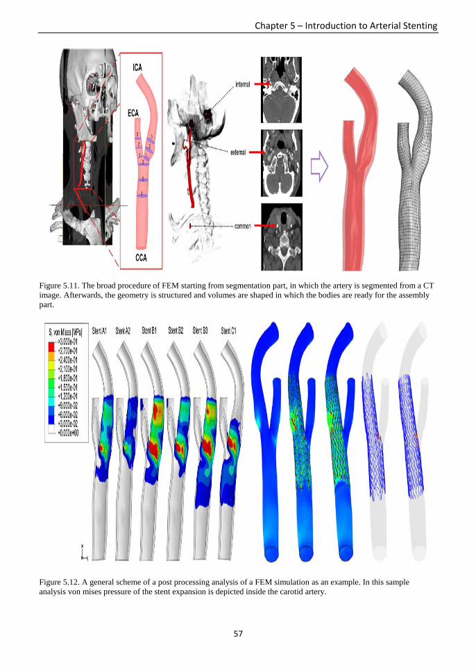
Chapter 5 – Introduction to Arterial Stenting
57
Figure 5.11. The broad procedure of FEM starting from segmentation part, in which the artery is segmented from a CT
image. Afterwards, the geometry is structured and volumes are shaped in which the bodies are ready for the assembly
part.
Figure 5.12. A general scheme of a post processing analysis of a FEM simulation as an example. In this sample
analysis von mises pressure of the stent expansion is depicted inside the carotid artery.

Chapter 5 – Introduction to Arterial Stenting
58
5.5. Problems and aims of the work
Two major problems exist in CAS angioplasty: (i)elastic and small plaques with early
calcifications penetrate into the stent leading to “plaque protrusion”(Figure 5.13-(a)). (ii)stiff and
large caps which contain advanced calcifications when being pushed by the stent/balloon lead to
eventual arterial wall rupture or stent fracture during the operation (Figure 5.13-(b)).
Investigation on clinical as well as mechanical behavior of fibrous cap, lipid pools and different
arterial layers have been extensively performed [54], [55], however there is lack of probe into
association of calcification and physiological phenomena that occurs during the development of
atherosclerosis as well as susceptibility of the carotid plaque during CAS angioplasty. The aim of
this work is to particularly explore on contribution of calcification in atherosclerotic plaque
rupture and to find its maximum resistance when imposed by external pressure load during
interventional CAS placement by exploiting Agatston Calcium score.
In this work, we performed a virtual simulation exploiting FEM to design a patient-specific pre-
operative framework in order to predict the interaction of main objects i.e. balloon, stent,
calcified plaque and artery in CAS operation. In order to achieve this goal, we followed two
approaches; (i)we obtained mechanical parameters imposed by balloon and stent on calcifications
during CAS placement through a nonlinear static structural analysis to elaborate about plaque
penetration and rupture characteristics. (ii)to find the nonlinear correlation between material
properties of the calcification i.e. Ca score, elasticity, and its obtained mechanical properties i.e.
equivalent stress, strains and ultimate external load in an imposed configuration. Teng et al. [38]
statistically investigated on carotid atherosclerotic plaque progression measured by wall thickness
increase (WTI) on in vivo Magnetic Resonance Imaging (MRI) data and found a negative
correlation between WTI and plaque wall stress confirming the fact that increase in plaque size
leads to lower flow wall shear stress. They also performed regression analysis to define a model
for predicting a patient-specific quantitative plaque growth functions. However both correlation
and regression analyses are linearly performed.
In the current study, we innovatively analyzed plastic behaviors of calcification and arterial wall
in additional to linear elastic properties. However, in reality large calcifications with high Ca
score could act as a ductile elastic material and conversely, calcifications with both small volume
and Ca score might behave as hard brittle material, hence it is not trivial to non-experimentally
classify the calcifications base on its hardness through the material properties. Therefore, we
defined inter-patient densities for each calcification as a novelty, considering them as
inhomogeneous material hence categorizing them by their elastic modulus.
(a)

Chapter 5 – Introduction to Arterial Stenting
59
(b)
Figure 5.13. (a) When the stent is too much open, the plaque is smashed and penetrated into the stent leading to plaque
protrusion. (b) When the stent is expanding, hardness of the plaque prevents the stent to open completely leads to
plaque and arterial vulnerability.
This section of the work is organized as follows:
In Chapter 5 we introduced and explained general concepts of atherosclerosis and calcified
carotid plaques and the mode of its evaluation using Agatston score. Then whole general
procedure of carotid artery stenting is explained in detail. In order to become acquaintance with
the investigated parameters and the way to probe the plaque rupture we introduced material and
mechanical parameters exploited to analysis the plaque rupture. Finally we stated some general
procedure of Finite Element Analysis in order to deploy the method in simulation and obtaining
in silico results.
In chapter 6 the material and method of the work is explained in detail. The method to data
acquisition is stated first and the model to design and reconstruction both calcification and
balloon/stents are explained in elaboration. The final part of this chapter is dedicated to exploiting
FEM in our method.
In chapter 7, the results that are obtained through both imposing balloon and stent on the
calcification belonging to each patient are presented. In addition to mechanical and material
parameters that are obtained we performed nonlinear statistical analysis to find the correlation
between the parameters.
Eventually in chapter 8, the final chapter we presented discussion and conclusion about our work
along with the future work.

Chapter 6 – Materials and Methods
60
Chapter 6 : Materials and Methods

Chapter 6 – Materials and Methods
61
6.1. Data Acquisitions
A total of 148 carotid bifurcations belonging to 74 patients (mean age 72.7 ± 6.6 years,
male:female=69:5) were acquired. MDCT angiography was performed in all study patients using
helical acquisition with a 64-detector row CT scanner (SOMATOM Definition; Siemens Medical
Solutions, Forchheim, Germany) with two X-ray tubes mounted onto a single gantry at an angle
of 90° as described previously [46]. The imaging acquisition parameters were as follows: spiral
mode 0.33-second gantry rotation; collimation, 32 x 0.6 mm; pitch factor, 1.5; section thickness
1.0 mm; reconstruction interval, 0.5 mm, and acquisition parameters 120 kVp and 350 mA. A
total 50 ml of non-ionized contrast medium, iohexol (Omnipaque 300; Daiichi Sankyo, Tokyo,
Japan) or iopamidol (Iopamiron 300; Bayer Schering Pharma, Berlin, Germany), was injected at
a flow rate of 3.5 ml/s, followed by 25 ml of a saline chaser at the same rate as the contrast
medium. Optimal timing of MDCT angiography acquisition was determined by an automated
bolus-timing program. Images were obtained from the aortic arch to the level of the inferior
orbits. The image data were transferred to a computer workstation (Ziostation version 1.17;
Amin, Tokyo, Japan) for image post-processing and calcification of the carotid plaque was
quantified. The Agatston calcium score [47] of any calcification area >1 mm2 with attenuation
≥130 Hounsfield units (HU) was determined by multiplying lesion area (total number of pixels)
by the cofactor 1–4 (cofactor 1; 130–199 HU, cofactor 2; 200–299 HU, cofactor 3; 300–399 HU,
cofactor 4; ≥400 HU) with non–contrast-enhanced CT obtain before contrast media injection for
CT angiography. Calcium was further quantified in cubic millimeters with the volume score
calculated as the product of voxel volume and number of voxels in the region of interest and the
overall calcium score of the plaque was the sum of the values for all individual lesions [48]. All
the carotid bifurcations have gone under surgical interventions by CAS, including 4 restenosis
cases. The ethics guidelines for clinical studies by the Japanese Health Labor and Welfare
Ministry (2003) were strictly observed.
6.2. Calcification model reconstruction
Among all the bifurcations, 20 cases were chosen for three dimensional experimental simulations
with average Ca score and calcified area of 400±510 and 84.2±77.1 mm2 respectively. Average
peak HU is 835±351. Table 1 represents material properties of calcifications ordered from the
highest Ca score to the lowest. Cases with a fair dispersion of Ca score along with similar
geometry and volume score are chosen in order to prevent dependency of the final results on
extensiveness of local geometry. The reason in which distribution of volume score and area of the
calcifications does not coincide is that volume score is calculated based on all the lesions inside
the carotid artery, however area belongs to one or two calcifications chosen among all the lesions
depending on the case, hence area is single calcification specific.
We defined different densities for each calcification, since calcified plaques are inhomogeneous
and material substantial are irregularly distributed over the plaque, thus some parts are denser
than the other parts. With respect to our previous work [46] 81.3% of calcified plaque with
Volume Score >500 mm3, have larger differences between peak and mean HU, indicating that
larger calcifications tend to be more inhomogeneous. Therefore by defining different densities,
we experience a virtual configuration which is close to reality. We considered calcified plaques
as inhomogeneous but isotropic material for two reasons: (i)we assume tensile and compressive
tensions imposed on the materials are equal on all the directions. (ii)complexity in analyzing
anisotropic mechanical behavior for inhomogeneous materials.
In order to define material properties for calcifications, an equation is required to numerically
express the available energy in fracture of vulnerable plaques. Consequently, a stress-strain curve
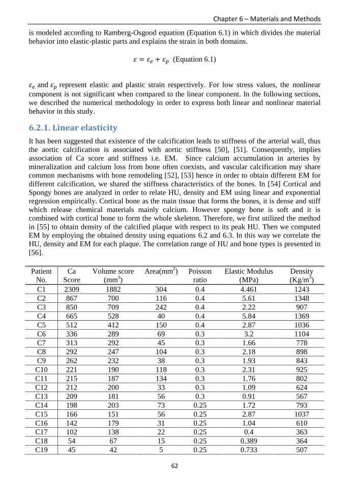
Chapter 6 – Materials and Methods
62
is modeled according to Ramberg-Osgood equation (Equation 6.1) in which divides the material
behavior into elastic-plastic parts and explains the strain in both domains.
휀 = 휀𝑒 + 휀𝑝 (Equation 6.1)
휀𝑒 and 휀𝑝 represent elastic and plastic strain respectively. For low stress values, the nonlinear
component is not significant when compared to the linear component. In the following sections,
we described the numerical methodology in order to express both linear and nonlinear material
behavior in this study.
6.2.1. Linear elasticity
It has been suggested that existence of the calcification leads to stiffness of the arterial wall, thus
the aortic calcification is associated with aortic stiffness [50], [51]. Consequently, implies
association of Ca score and stiffness i.e. EM. Since calcium accumulation in arteries by
mineralization and calcium loss from bone often coexists, and vascular calcification may share
common mechanisms with bone remodeling [52], [53] hence in order to obtain different EM for
different calcification, we shared the stiffness characteristics of the bones. In [54] Cortical and
Spongy bones are analyzed in order to relate HU, density and EM using linear and exponential
regression empirically. Cortical bone as the main tissue that forms the bones, it is dense and stiff
which release chemical materials mainly calcium. However spongy bone is soft and it is
combined with cortical bone to form the whole skeleton. Therefore, we first utilized the method
in [55] to obtain density of the calcified plaque with respect to its peak HU. Then we computed
EM by employing the obtained density using equations 6.2 and 6.3. In this way we correlate the
HU, density and EM for each plaque. The correlation range of HU and bone types is presented in
[56].
Patient
No.
Ca
Score
Volume score
(mm3)
Area(mm2) Poisson
ratio
Elastic Modulus
(MPa)
Density
(Kg/m3)
C1 2309 1882 304 0.4 4.461 1243
C2 867 700 116 0.4 5.61 1348
C3 850 709 242 0.4 2.22 907
C4 665 528 40 0.4 5.84 1369
C5 512 412 150 0.4 2.87 1036
C6 336 289 69 0.3 3.2 1104
C7 313 292 45 0.3 1.66 778
C8 292 247 104 0.3 2.18 898
C9 262 232 38 0.3 1.93 843
C10 221 190 118 0.3 2.31 925
C11 215 187 134 0.3 1.76 802
C12 212 200 33 0.3 1.09 624
C13 209 181 56 0.3 0.91 567
C14 198 203 73 0.25 1.72 793
C15 166 151 56 0.25 2.87 1037
C16 142 179 31 0.25 1.04 610
C17 102 138 22 0.25 0.4 363
C18 54 67 15 0.25 0.389 364
C19 45 42 5 0.25 0.733 507

Chapter 6 – Materials and Methods
63
C20 31 40 33 0.25 0.381 360
AVG 400 343 84.2 - 2.17 823
SD 510 408 77.1 - 1.6 310 Table 6.1. Material properties belong to all the calcifications in this study ordered from the highest to the lowest Ca
score. patient-specific elastic modulus and density are also presented.
𝐻𝑈 ≥ 1200 → Considered as Cortical bone,
𝐸 = 0.011 × 𝜌 − 9.212 (Equation 6.2)
100 ≤ 𝐻𝑈 ≤ 1200 → Considered as Spongy bone,
𝐸 = 0.005 × 𝜌^1.91 (Equation 6.3)
ρ represents density and E is elastic modulus. HU is considered as peak HU. All the EM for the
calcified plaques are assigned based on the latter equations. Average of calculated EM and
density are 2.17±1.6 MPa and 823±310 Kg/m3 respectively. In Table 6.1, EM and density
calculated for each patient is summarized. In chapter 8 correlation of Ca score and EM has been
debated.
6.2.2. Nonlinear plasticity
The goal to investigate nonlinear behavior of a material is to obtain ultimate tensile strength
(UTS) and strain at break. Utilizing FEM the idea is to apply the external loads on inner surface
of both stent and balloon to expand and press the calcification while the internal stress of
calcification cross the yield point. At this point plastic deformation starts and eventually
calcification reaches to UTS and breaks. We performed sensitivity analysis on the external
pressure load to find maximum allowed external pressure on each calcification and obtain the
ultimate mechanical parameters at rupture. However in order to apply abovementioned
simulation we required tangent modulus (TM) which we defined as slope of nonlinear domain
after the yield point (𝜎𝑦) and then depending on applied forces on cross-sectional region of
interest, desired ultimate parameters are achieved. Figure 6.1 expresses stress-strain curve
obtained after stent simulation for calcification case 1.
Figure 6.1. Stress-strain curve belong to calcification of case 1. 𝜎𝑦 is yield stress that plastic deformation begins.
EM (𝐸) and TM (𝐸𝑡) have been pointed along with 휀𝑒 and 휀𝑝 that represent elastic and plastic strain.
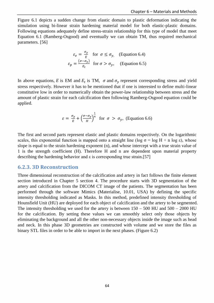
Chapter 6 – Materials and Methods
64
Figure 6.1 depicts a sudden change from elastic domain to plastic deformation indicating the
simulation using bi-linear strain hardening material model for both elastic-plastic domains.
Following equations adequately define stress-strain relationship for this type of model that meet
Equation 6.1 (Ramberg-Osgood) and eventually we can obtain TM, thus required mechanical
parameters. [56]
휀𝑒 = 𝜎𝑦
𝐸 for 𝜎 ≤ 𝜎𝑦, (Equation 6.4)
휀𝑝 =(𝜎−𝜎𝑦)
𝐸𝑡 for 𝜎 > 𝜎𝑦, (Equation 6.5)
In above equations, 𝐸 is EM and 𝐸𝑡 is TM, 𝜎 and 𝜎𝑦 represent corresponding stress and yield
stress respectively. However it has to be mentioned that if one is interested to define multi-linear
constitutive low in order to numerically obtain the power-law relationship between stress and the
amount of plastic strain for each calcification then following Ramberg-Osgood equation could be
applied.
휀 = 𝜎𝑦
𝐸+ (
𝜎−𝜎𝑦
𝐻)
1
𝑛 for 𝜎 > 𝜎𝑦, (Equation 6.6)
The first and second parts represent elastic and plastic domains respectively. On the logarithmic
scales, this exponential function is mapped onto a straight line (log σ = log H + n log ε), whose
slope is equal to the strain hardening exponent (n), and whose intercept with a true strain value of
1 is the strength coefficient (H). Therefore H and n are dependent upon material property
describing the hardening behavior and ε is corresponding true strain.[57]
6.2.3. 3D Reconstruction
Three dimensional reconstruction of the calcification and artery in fact follows the finite element
section introduced in Chapter 5 section 4. The procedure starts with 3D segmentation of the
artery and calcification from the DICOM CT image of the patients. The segmentation has been
performed through the software Mimics (Materialise, 10.01, USA) by defining the specific
intensity thresholding indicated as Masks. In this method, predefined intensity thresholding of
Hounsfield Unit (HU) are deployed for each object of calcification and the artery to be segmented.
The intensity thresholding we used for the artery is between 150 – 500 HU and 500 – 2000 HU
for the calcification. By setting these values we can smoothly select only those objects by
eliminating the background and all the other non-necessary objects inside the image such as head
and neck. In this phase 3D geometries are constructed with volume and we store the files as
binary STL files in order to be able to import in the next phases. (Figure 6.2)
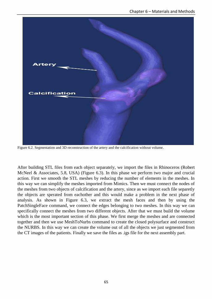
Chapter 6 – Materials and Methods
65
Figure 6.2. Segmentation and 3D reconstruction of the artery and the calcification without volume.
After building STL files from each object separately, we import the files in Rhinoceros (Robert
McNeel & Associates, 5.8, USA) (Figure 6.3). In this phase we perform two major and crucial
action. First we smooth the STL meshes by reducing the number of elements in the meshes. In
this way we can simplify the meshes imported from Mimics. Then we must connect the nodes of
the meshes from two objects of calcification and the artery, since as we import each file separetly
the objects are sperated from eachother and this would make a problem in the next phase of
analysis. As shown in Figure 6.3, we extract the mesh faces and then by using the
PatchSingleFace command, we connect the edges belonging to two meshes. In this way we can
specifically connect the meshes from two different objects. After that we must build the volume
which is the most important section of this phase. We first merge the meshes and are connected
together and then we use MeshToNurbs command to create the closed polysurface and construct
the NURBS. In this way we can create the volume out of all the objects we just segmented from
the CT images of the patients. Finally we save the files as .igs file for the next assembly part.

Chapter 6 – Materials and Methods
66
Figure 6.3. Connecting the meshes belonging to calcification and the artery in Rhinoceros.
The next phase is the assembly part. We must assemble and merge the previously designed stents
and the balloon inside the arterial calcification. We perform this action using Solidworks
(Dassault Systèmes SolidWorks Corp., 2013, Vélizy, France). The .igs file is imported and
assembly is performed. The exact geometry and the distances are explained in the parts 6-3-1 and
6-4 in details. Figure 6.4 depicts the assembly of two stents models fixed on the calcification
inside the artery.
Figure 6.4. Assembly of two stent models resided on the calcification inside the artery using a specific geometry.

Chapter 6 – Materials and Methods
67
The final phase of 3D reconstruction belong to importing the designed assembly into geometry
section of the Ansys (Ansys, Inc. 15.0, USA) in which it is employed for the main FEM analysis
and obtaining the final mechanical parameters. Figure 6.5 below depicts the imported assembled
stents, artery and calcification.
Figure 6.5. Assembled layout belongs to a case in which the stents is resided on the calcification inside the artery.
6.3. Balloon/Stent model reconstruction
We analyzed elastic-plastic material behavior of balloon/stents/artery and calcifications, thus
Elastic Modulus (EM) and Poisson Ratio are defined to characterize linear elastic stiffness and
compressibility for each calcified plaque. On the other hand to characterize the nonlinear plastic
behavior, we defined slope of the curve after the yield point in the stress-strain curve as Tangent
Modulus (TM). Two types of stents and one type of pre-stenting balloon are deployed in the
simulations. Modeled stents are both carotid self-expandable open-cell and close-cell stent
depending on the model of bifurcations. We chose the cases as such two types of stents are fairly
included. Open cell stent belongs to Cordis Corporation registered as PRECISE® PRO RX®.
The material is Nitinol alloy with geometry property of maximum expansion of 6~10 mm, 40 mm
length and cell size of 2 mm and fits to extremely tortuous vessels. On the other hand, closed-cell
stent is Carotid WALLSTENT® Monorail® from Boston Scientific. The material is stainless
steel Elgiloy composed of DFT (Draw Filed Tubing) alloy monofilament wires braided in a
tubular mesh configuration. The stent has 10 mm in diameter and 40 mm length which fits to
unstable plaque morphology. Average arterial diameter for our experiments is 8~10 mm and the
average calcification diameter is 0.5~7 mm and since the chosen stents should be 1~2 mm wider
than the artery, the geometrical parameters are carefully chosen. Average calcification thickness
is 95𝜇𝑚. We deployed Sterling pre-stenting dilation balloon from Boston Scientific. It is made of
compressible elastoplastic material with very low friction coefficient composed of Polyether
block Amide (PDA) leading to atraumatic lesion entry with diameter of 3.5 mm and 40 mm
length. In Table 6.2 all the material properties for the artery, angioplasty balloon and two utilized
stents are presented.

Chapter 6 – Materials and Methods
68
Material
property
Elastic
Modulus
(MPa)
Poisson
ratio
Yield
Strength
(MPa)
Tangent
Modulus
(MPa)
Density
(Kg/m3)
Heat
capacity
(J/Kg.C)
Artery 1.75 0.49 1.1 0.9 1000 300
Sterling
Balloon
513 0.27 56 85 1010 1700
Precise Stent 28000 0.3 100 800 6450 320
Wallstent
Stent
189600 0.226 480 900 8300 430
Table 6.2. Utilized material properties for artery, balloon and two stents.
In the following Table 6.3 we present very useful and important information for each patient on
type of stents, balloon number of voxels of calcification in the images, the side of carotid artery
that has the crucial stenosis, size of the stents and the balloon and finally the amount of pressure
and time on imposing the balloon by the real cardiologists.
No. Side Voxel Stent Size (mm) Balloon Pre-dilatation Size (mm) atm sec
1 L 2917 Precise 8x40 Sterling 3x40 6 30
2 L 1118 Precise 10x40 Sterling 3.5x40 6 30
3 R 1137 Wallstent 10x31 Sterling 3.5x40 6 30
4 L 831 Precise 8x40 Sterling 3x40 6 30
5 L 567 Wallstent 8x29 Sterling 3.5x40 6 30
6 R 474 Precise 8x40+8x30 Sterling 3x40 6 30
7 R 494 Wallstent 10x40 Sterling 3x40 6 30
8 R 388 Precise 8x40 Sterling 3.5x20 6 30
9 R 369 Wallstent 8x21 Sterling 3x30 6 30
10 R 291 Wallstent 10x24 Sterling 3x30 6 30
11 R 256 Precise 10x40 AMIIA 4x30 10 30
12 R 432 Wallstent 10x31 Sterling 3x40 6 30
13 R 388 Precise 7x40 Sterling 3x40 6 30
14 R 305 Wallstent 10x24 Sterling 3x30 6 30
15 R 245 Precise 7x40 Sterling 3x20 6 30
16 R 307 Precise 10x40 Sterling 3x40 6 30
17 L 251 Precise 10x40 Sterling 3x30 6 30
18 L 147 Wallstent 8x29 - - - -
19 R 88 Wallstent 8x29 Sterling 3x40 6 30
20 L 71 Wallstent 10x31 Sterling 3.5x40 6 30 Table 6.3. Clinical information belonging to all the patients.

Chapter 6 – Materials and Methods
69
6.3.1. 3D reconstruction
3D reconstruction of the deployed balloon and two open-cell and closed-cell stents exactly
follows the geometrical section of FEM already explained in Section 6-2 belonging to design of
calcification and the artery. Except that we did not segment or extract the stents and balloon from
the CT images. We designed using CAD software of Solidworks with respect to the geometry
parameters presented in the previous section. Therefore, here we only present the final
constructed images of the balloon and the stents in the following Figure 6.6.
Figure 6.6. Sterling Balloon (A) and two stents: Closed-cell Wallstent (B) and Open-cell Precise (C) three dimensional
design.
6.4. Finite Element Analysis and Simulation
An advanced interventional endovascular CAS angioplasty consists of three steps that starts with
pre-dilation balloon to open the artery and pushes the plaque followed by self-expandable
stenting that fits to the arterial wall and finally post-dilation balloon placement in order to adjust
the previously expanded stent. In this study we performed a patient-specific modeling and
simulation for the balloon and stent expansion as a separated structural configuration. Therefore,
we performed two independent FEM simulations for balloon and stent. In many cases of previous
studies the “failure” is defined as the ultimate fracture of the whole plaque [59], [60], however
we defined the “failure” as initial intimal plaque rupture. Since, “vulnerable” is defined as a
considerable amount of internal stress resisting the break, thus vulnerability has direct correlation
with the stress imposed on calcification [60]. Therefore if the plaque has a part protruded or
indented then the failure could happen from that part in which we take the ultimate internal stress
of the calcification into consideration at that moment.
The whole technical workflow starts with segmentation of the arteries from DICOM CT images
using Mimics (Materialise, 10.01, USA). Among all the lesions inside the artery, depending on
local geometry, location and feasibility of stenting we chose one or two calcified plaque for
segmentation. Selected lesions are mostly resided inside or in the entry of ICA bifurcation.
Reconstructed geometry is stored as an STL file in order to apply thickness and volume in the
next step. Calcifications inside the left carotid artery are visible in CT image of a patient in
Figure 6.7.

Chapter 6 – Materials and Methods
70
(a) (b) (c)
Figure 6.7. CT image belongs to a case where left carotid artery along with the calcifications are visible. Both artery
and the calcified plaque are segmented for further construction in coronary (a), saggital (b) and axial view (c).
Three dimensional open surface geometry is constructed as STL which using Rhinoceros (Robert
McNeel & Associates, 5.8, USA) it is converted to a closed polysurface volume or solid NURBS.
Since STL file is made of a triangular mesh, after volume creation, arterial body and the calcified
plaque is detached. By using merge mesh methods, we connect the meshes in order to prevent the
cavity that is emerged between the plaque and the arterial wall. Final volumes are stored as IGS
files in order to be imported in the assembly part. Followed by arterial segmentation and
reconstruction, we designed the balloon (Figure 6.6-A) and two stents models (Figure 6.6-B, C)
deploying predefined geometry properties presented in section II.B. We then assembled artery
and calcification volumes with the modeled stents and balloon according to the patient data by
employing Solidworks (Dassault Systèmes SolidWorks Corp., 2013, Vélizy, France). As shown
in Figure 6.6, balloon and stents are designed fixed above the calcification and spaced 0.15 mm
from the surface.
FEA is performed through commercially available software Ansys (Ansys, Inc. 15.0, USA). We
used nonlinear static structural analysis to perform the simulation, due to simplicity in analysis by
applying structural loads and neglecting inertial forces. Likewise we looked into a global
response of the structural system by assuming the loads for both balloon and stent placement over
>1s of time. Utilizing FEA application consists of three major procedures. First material
properties are defined in which we employed nonlinear hardening material definition for artery,
calcification, stents and the balloon. Next geometry properties of each material are specified
through the configuration assembled previously. Arterial wall is extruded for 1 mm layer
thickness that represents three arterial layers i.e. intima, media and adventitia. One of the most
important criteria which affect the final result is the distance of each calcification and the arterial
wall and it is completely patient-specific.
In the modeling, we defined boundary conditions to describe the simulation. The boundary
condition defined for balloon/stent is symmetrical in axial direction of the Cartesian coordinate
system in order to characterize evenly distributed loads and to force a symmetric expansion.
Cylindrical support is defined to confine the expansions only to axial and radial direction, but not
circumferential direction and prevent rigid body motion. We defined a frictional connection
between the balloon/stent and the calcified plaque with frictional coefficient of 0.2 for balloon-
plaque and 0.4 for stent-plaque respectively using Augmented Lagrange formulation that have
been obtained through sensitivity testing. Calcified plaques are in contact with the artery using a
bonded connection. Free displacement is applied on the calcified plaque since clinically it is free

Chapter 6 – Materials and Methods
71
to move in any direction as long as limited inside the arterial layers. On the other hand, fixed and
elastic support are defined for arterial walls, however it is allowed to stretch and having relatively
damping effect. Damping effect is given to the arterial wall by defining stiffness foundation of
0.1 N/mm3.
Loading condition is defined by applying external radial load on inner surface of balloon and
stents. Balloon expansion configuration is resembled as 6-10 atm of the pressure into the balloon
continuously pushing the calcified plaque for 30s. In terms of stent, since it is self-expandable, it
instantly opens soon as taken out from angioplasty catheter. Tetrahedrons patch conforming
meshing is utilized for the whole configuration with minimum element size of 0.1 mm for
calcification and 0.4 mm for other parts because of being less significant except the contact
region in which location-specific meshing configuration is applied for both contact and target
bodies. Figure 6.8 expresses mesh configurations of Case 4 for balloon/calcification. Panel (a)
shows finer mesh size for only the calcification comparing to panel (b) with coarser mesh.
Results for both mesh size have been described in chapter 7.
(a) (b)
Figure 6.8. Mesh view of balloon placed on calcification for Case C4. (a)Finer mesh size is utilized for the
calcification where (b)Coarser meshing has been defined for calcification. Mesh element size for balloon is coarser
comparing to calcification due to priority in importance of the objects in the analysis. Contacts area has the same mesh
configuration.
As mentioned before two types of coordinate systems are defined depending on types of loads
and supports that have been identified. Figure 6.9 shows two types of coordinate systems
comprises cylindrical system that is used for supports and confining the displacements of the
objects and Cartesian coordinate system to define loads and symmetrical boundary condition.
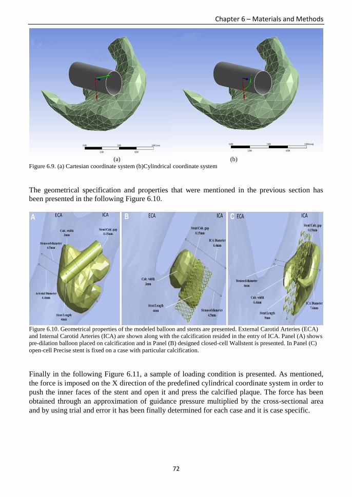
Chapter 6 – Materials and Methods
72
(a) (b)
Figure 6.9. (a) Cartesian coordinate system (b)Cylindrical coordinate system
The geometrical specification and properties that were mentioned in the previous section has
been presented in the following Figure 6.10.
Figure 6.10. Geometrical properties of the modeled balloon and stents are presented. External Carotid Arteries (ECA)
and Internal Carotid Arteries (ICA) are shown along with the calcification resided in the entry of ICA. Panel (A) shows
pre-dilation balloon placed on calcification and in Panel (B) designed closed-cell Wallstent is presented. In Panel (C)
open-cell Precise stent is fixed on a case with particular calcification.
Finally in the following Figure 6.11, a sample of loading condition is presented. As mentioned,
the force is imposed on the X direction of the predefined cylindrical coordinate system in order to
push the inner faces of the stent and open it and press the calcified plaque. The force has been
obtained through an approximation of guidance pressure multiplied by the cross-sectional area
and by using trial and error it has been finally determined for each case and it is case specific.

Chapter 6 – Materials and Methods
73
Figure 6.11. Loading condition defined on the inner surface of the stent to be pushed and opened. The force is imposed
on the x direction of the cylindrical coordinate in this case. The force has been obtained through an approximation of
guidance pressure multiplied by the cross-sectional area and by using trial and error it has been finally determined for
each case and it is case specific.

Chapter 7 – Results
74
Chapter 7 : Results

Chapter 7 – Results
75
7.1. Arterial Diversity
We demonstrated coronal view of carotid artery bifurcations belonging to twelve patients out of
twenty cases we acquired, categorized by the largest to smallest calcification directly segmented
from the CT images to show diversity in the local geometry (Figure 7.1). Diversity of the arterial
local geometry is evident in Figure 7.1, as such the largest calcifications are correlated with the
larger arteries.

Chapter 7 – Results
76
Figure 7.1. Overall coronal mesh view of the segmented arteries and calcification from CT images belonging to 12
cases out of 20 cases. Yellow objects express calcifications.
7.2. Plaque imposed by Balloon
Here mechanical parameters obtained from imposing balloon on calcified plaques are presented
in terms of both quantitative and qualitative results. Imposing the maximum and average ultimate
external pressure as 1.5MPa and 1.11 ± 0.31MPa to expand the balloon, we obtained the
maximum and average ultimate stress of 120kPa and 55.7 ± 41.2kPa on the calcifications
respectively. Average elastic and plastic strain were 0.03±0.02 and 0.006±0.01. We indicated
patient-specific Plaque Wall Stress (PWS) which was defined as shear stress on cross-sectional
area of arterial layer and calcification when is in dynamic contact with balloon/stent. Maximum
and average PWS was equal to 44kPa and 19.03±16.05kPa. TM is also calculated with respect to
obtained mechanical parameters using Equation 5 with average of 0.68±1.17MPa. Expanding the
balloon by imposing maximum external load, we did not encounter rupture in arterial wall
whereas except 3 cases with balloon rupture, all the other cases led to calcification break.
Next we statistically analyzed the relationship between material properties of the calcification i.e.
Ca score, EM and obtained mechanical parameters i.e. ultimate stress, PWS using nonlinear
Spearman’s correlation to find the most influential material characteristics in calcified plaque
rupture. However Ca score is obtained for all the lesions inside an artery, while EM is
calcification-specific, hence practically it conveys stronger correlation (See Chapter 8). Therefore
in Table 2 we summarized average values for each parameter and its correlation (indicated with
R) with EM. There was a strong positive correlation between EM and ultimate stress (0.58;
P=0.008) as well as EM and PWS (0.66; P=0.002). We can state that calcified plaques with
larger EM when imposed by maximum pressure, have higher ultimate stress and PWS,
consequently it is stiffer and more resistance to rupture.

Chapter 7 – Results
77
Parameters Average values Correlation with EM
Ultimate external force 1.11±0.31 MPa R= 0.62; p=0.005
Ultimate Stress 55.7±41.2 kPa R= 0.58; P=0.008
Plaque Wall Stress 19.03±16.05 kPa R= 0.66; P=0.002
Elastic Strain 0.03±0.02 R= -0.56; p=0.005
Table 7.1. Average mechanical parameters from balloon simulation and their correlation with elastic modulus.
(statistically significant threshold, p<0.05)
In Figure 7.2, scatter graph is plotted to demonstrate the relationship between EM and ultimate
stress/PWS for twenty data pairs imposed by balloon.
Figure 7.2. Scatter plot for EM v.s. ultimate stress and PWS for balloon analysis. Quadratic regression curves are also
depicted to fit the intercepts. Strong positive correlation is inferred from the graph.
In Table 7.2, mechanical parameters belong to all the cases that are obtained by calcified plaque
imposed by balloon are presented in the order of largest CA score to the smallest. The cases with
plastic strain equal to zero indicate that the nonlinear deformation has not reached through
balloon expansion, due to contacts and material properties of the balloon and each calcification.

Chapter 7 – Results
78
Patient
NO
Load at
break
(MPa)
Max von
mises stress
(KPa)
Max Elastic
strain(mm/mm
)
Plastic
strain(mm/m
m)
Tangent
Modulus
(MPa)
Plaque
Wall
stress
(KPa)
1 0.8 116 0.02 0.003 3.5 50
2 1.5 96.42 0.00 0.02 2.4 38.78
3 1.1 32.8 0.01 0 0 13.22
4 1.3 99.7 0.006 0.013 4.92 24.1
5 1.1 32.6 0.009 0 0 11
6 1.5 120 0.03 0 0 44
7 0.8 13 0.009 0.001 1.01 3.2
8 1.5 104 0.04 0 0 37
9 0.8 22 0.01 0 0 8.5
10 1.4 70 0.02 0 0 27.2
11 1.5 112 0.04 0.035 1.05 40.2
12 0.7 12 0.09 0 0 2.9
13 1.3 40 0.04 0 0 12.8
14 0.6 12 0.004 0.012 0.47 1.2
15 1.5 102 0.03 0 0 32.6
16 1.1 41.3 0.03 0.032 0.18 13.5
17 1 14 0.03 0 0 3.3
18 1 34 0.08 0.009 0.33 7.7
19 1.1 32 0.04 0.002 0.9 9.6
20 0.6 10 0.02 0 0 1.26
Avg 1.11 53.36 0.063 0.035 0.68 19.03
Table 7.2. Mechanical parameters obtained for each patient by imposing balloon on the calcified plaque.
Finally we presented quantitative analysis of all the obtained mechanical parameters from
imposing loads on calcification by balloon in the following graphs. The graphs in Figure 7.3
represent (a)ultimate stress, (b)PWS, (c)elastic, (d)deformation and (e)plastic strain came from
outcome of 12 cases. In Figure 7.3 panel (f) we also presented the standardized amount of Ca
score and ultimate stress in order to show the standardized normal correlation between two
parameters. As can be seen, most of the cases have direct correlation between Ca score and
ultimate stress.

Chapter 7 – Results
79
(a) (b)
(c) (d)
(e) (f)
Figure 7.3. Mechanical parameters of (a)ultimate stress (b)PWS(c)Elastic strain(d)Deformation(e)Plastic
strain(f)standardized Ca score and ultimate stress for 12 cases imposed by balloon.
0
20
40
60
80
100
120
1 2 3 4 5 6 7 8 9 10 11 12
Stre
es
(KP
a)
Stress by Balloon
0
5
10
15
20
25
30
1 2 3 4 5 6 7 8 9 10 11 12
PWS by Balloon
0
0.02
0.04
0.06
0.08
0.1
0.12
0.14
0.16
1 2 3 4 5 6 7 8 9 10 11 12
Elastic Strain by Balloon
0
0.1
0.2
0.3
0.4
0.5
0.6
1 2 3 4 5 6 7 8 9 10 11 12
Deformation by Balloon
0
0.0001
0.0002
0.0003
0.0004
0.0005
0.0006
1 2 3 4 5 6 7 8 9 10 11 12
Plastic Strain by balloon
-1.5
-1
-0.5
0
0.5
1
1.5
2
2.5
3
3.5
1 2 3 4 5 6 7 8 9 10 11 12
Ca Std Stress STD

Chapter 7 – Results
80
7.3. Plaque imposed by stent
The same analysis has been performed for both open-cell and closed-cell stents to find the
maximum pressure imposed on stent and ultimate parameters of the calcified plaques.
Quantitatively, ultimate stress on the calcifications is increased notably comparing to balloon
expansion. Since the ultimate stress is dependent upon material of contact object, surface friction,
temperature, therefore number of calcified plaque reached to plastic domain is increased.
Maximum and average ultimate stresses were 492kPa and 171±145kPa respectively. Maximum
and average ultimate external load at break were obtained as 4.2MPa and 2.32 ±1.16MPa
obviously showing a huge difference comparing to balloon. PWS caused by stent expansion were
208kPa and 64.3±63.3kPa for maximum and average values. We obtained average elastic and
plastic strain as 0.08±0.06 and 0.03±0.04 which were significantly increased due to stent
interaction. We specifically computed the penetration of the stent inside the calcification with
average of 0.03±0.04mm in which helps in calculation of patient-specific plaque protrusion.
Slope of the plastic deformation (TM) was increased to 1.19±1.47MPa. Table 7.3 shows the
average values for each mechanical parameters and their correlation with EM. The Spearman’s
coefficient between EM and external load was significantly increased to 0.71 (p=0.001).
Likewise correlation between EM and ultimate stress and then PWS were 0.85 (p<0.0001) and
0.92 (p<0.0001) respectively, which comparing to balloon we obtained much stronger and
positive correlation. We can infer the same interpretation for balloon here as the higher the EM of
the calcification, higher the ultimate stress hence less susceptible to rupture. Scatterplot in Figure
7.4 depicts the stronger relationship comparing to the balloon between EM and ultimate
stress/PWS.
Parameters Average values Correlation with EM
Ultimate external force 2.32±1.16 MPa R= 0.71; p=0.001
Ultimate Stress 171±145 kPa R= 0.85; p<0.0001
Plaque Wall Stress 64.3±63.3 kPa R= 0.92; p<0.0001
Elastic Strain 0.08±0.06 R= -0.72; p<0.0001
Table 7.3. Average values for mechanical parameters obtained from stent simulation and their nonlinear spearman’s
correlation with elastic modulus. (statistically significant threshold, p<0.05).

Chapter 7 – Results
81
Figure 7.4. Scatter plot for EM v.s. ultimate stress and PWS for stent simulation. Quadratic regression curves show
better data fit for stent analysis whereas comparing to balloon expansion monotonic pattern is well demonstrated.
In Table 7.4, mechanical parameters belong to all the cases that are obtained by calcified plaque
imposed by stent are presented in the order of largest CA score to the smallest. The cases with
plastic strain equal to zero indicate that the nonlinear deformation has not reached through
balloon expansion, due to contacts and material properties of the balloon and each calcification.
Comparing to balloon expansion, values for the stress/strain and TM are significantly increased
and this proves the fact that the ultimate mechanical parameters strictly depends on contacts,
material properties and cross-sectional area of the objects being in contact with eachother.

Chapter 7 – Results
82
Pati
ent
No
Load at
break
(MPa)
Max von
mises stress
(before
break) (KPa)
Max elastic
strain
(mm/mm)
Plastic
strain
(mm/mm
)
Max
Penetration
of stent in
Plaque (mm)
Tangen
t
Modul
us
(MPa)
Plaque
Wall
stress
52 3 112.23 0.0241 0.0027 0.000543 1.95 49.9
33 4.2 344.91 0.029168 0.04280 0.000243 4.3 139.143
68 1.5 49.372
0.021177 0.00000 0.004769 0 16.3016
3
37 3 198 0.024929 0.012 0.000933 4.83 66.577
71 2.7 147.68 0.051179 0.00136 0.000066 1 41
26 3.8 428.97 0.033593 0.0130 0.000222 2.48 208.615
58 2 100
0.081456 0.02657 0.011476 0.61 40.0290
6
16 3.5 396 0.066092 0.1070 0.004655 2.53 134
45 1.5 140 0.070274 0.0090 0.014777 0.5 35
56 2.5 217 0.040084 0.0950 0.000239 1.37 63.1
13 3.8 300 0.150390 0.05530 0.015324 0.72 141
59 0.8 29.2 0.025195 0.00000 0.012300 0 2
61 3 96.986 0.094760 0.02570 0.025589 0.64 45.9
44 1.3 25.3 0.013256 0.00000 0.022230 0 0
19 4 492 0.051000 0.13600 0.000935 2.66 176
54 1 135 0.132130 0.08800 0.011626 0.125 35
22 0.9 13.491 0.151075 0.00000 0.121930 0 3.59
66 1 26.87 0.205180 0.00000 0.200000 0 5.16
73 1.7 124 0.147660 0.09280 0.246710 0.184 44
67 1.2 53 0.250000 0.00000 0.021174 0 27.1
Ave
rage 2.32 169.8505 1.03E-01 4.41E-02 2.13E-02
1.19
64
Std_
dev
1.16148
7 147.3035 0.060927 0.048578 0.05943
1.47 59.8328
5 Table 7.4. Mechanical parameters obtained for each patient by imposing balloon on the calcified plaque.
Eventually in this section, we presented quantitative analysis of all the obtained mechanical
parameters from imposing loads on calcification by the stents in the following graphs. Figure 7.5,
represent (a)ultimate stress, (b)PWS, (a)elastic, (d)deformation and (e)plastic strain came from
outcome of 12 cases.
Chapter 7 – Results
83
(a) (b)
(a) (b)
(e)
Figure 7.5. Mechanical parameters of (a)ultimate stress (b)PWS(c)Elastic strain(d)Deformation(e)Plastic strain for 12
cases imposed by stents.
0
20
40
60
80
100
120
140
160
1 2 3 4 5 6 7 8 9 10 11 12
Stress by stent
0
10
20
30
40
50
60
70
80
1 2 3 4 5 6 7 8 9 10 11 12
Shear Stress by stent
0
0.02
0.04
0.06
0.08
0.1
0.12
0.14
0.16
1 2 3 4 5 6 7 8 9 10 11 12
Elastic Strain by stent
0
0.1
0.2
0.3
0.4
0.5
0.6
1 2 3 4 5 6 7 8 9 10 11 12
Deformation by stent
0
0.02
0.04
0.06
0.08
0.1
1 2 3 4 5 6 7 8 9 10 11 12
Plastic Strain by stent

Chapter 7 – Results
84
Finally for qualitative evaluation, we presented stress-strain analysis of the calcification imposed
by balloon for a case in Figure 7.6. Panel A shows maximum Von mises stress of the calcified
plaque resided in the entrance of internal carotid artery after being pushed by balloon. Panels B
and C illustrate elastic strain and plastic strain distributed over the calcification respectively. In
panel A position of the balloon, ICA, ECA and arterial wall thickness have been specified.
Figure 7.7, Top panel A shows UTS as Von mises stress where panel B presents PWS. Panel C
demonstrates both plaque/stent rupture in which due to large stiffness of the calcification higher
stress level is reached.
Figure 7.6. Stress-strain analysis for C4. Panel A shows Von mises stress distributed over the surface of the calcified
plaque. Expanded balloon is pointed along with the ICA, ECA and wall thickness. Panel B represents elastic strain.
Left color bar for strain distribution corresponds to the maximum values in Table 7.4. Panel C belongs to nonlinear
plastic deformation occurred in the center of dynamic interaction between balloon and calcification.
Figure 7.7. Stress-strain analysis belongs to C10. Panel A represents Von mises stress distribution due to wallstent
expansion which has been pointed. Panel B shows WSS on the arterial wall. In panel C we presented plaque and stent
break due to stiffness of the calcification in which causes to cross the UTS and fail.

Chapter 7 – Results
85
Finally for qualitative evaluation, we presented stress-strain analysis of the calcification imposed
by both balloon and stent for three different cases in Figure 7.8. Panel A shows maximum
ultimate stress of the calcified plaque in the entrance of internal carotid artery after being stented
by Wallstent. Panel B illustrates PWS shear stress induced between balloon/arterial wall and
calcification. For each case arterial wall thickness is visible in which the calcification is resided
under. In panel C we presented plastic strain started from the middle of calcification while
stented by Precise stent. Case in panel C is one the rare cases with stent break by having high TM
equal to 4.92MPa leading to a stiffer plasticity. Length of the stents and balloon is case-specific
and determined according to the cross-sectional area of the calcifications and stent/balloon for
simplicity in the calculation. In Figure 7.9 we presented qualitative analysis of both plaque
protrusion and plaque rupture. Panel A shows deformation values in a soft calcification where the
stent is penetrated inside due to high elasticity of calcification. Panels B and C demonstrate
fracture in plaque and stent in which due to large stiffness of the calcification, maximum stress
level is reached. The ultimate stress value and its locations after the rupture are indicted in the
images.
Figure 7.8. Stress-strain analysis of three different cases imposed by balloon and stent. Panel (A) shows equivalent
stress from center of the calcification while pressed by closed-cell stent. Panel (B) demonstrates PWS of a calcification
on balloon case and Panel (C) represents plastic-strain imposed by closed-cell stent on a case.

Chapter 7 – Results
86
Figure 7.9. Plaque protrusion and rupture are simulated by inducing the ultimate pressure on the stents. Panel (A)
shows the plaque is penetrated inside the stent. Panel (B) and (C) demonstrate soft plaque break due to 140kPa and
30kPa of the ultimate stress that crossed the maximum resistance of the calcification.
Finally for the qualitative evaluation, Figure 7.10 shows mechanical parameters obtained on three
different cases all by balloon expansion. In panel (a) ultimate stress as equivalent von mises
stress is visible in the bottom of calcification when pushed by the balloon. The contact between
the arterial layer and the bottom layer of calcification has the largest load. Panel (b), shear stress
between calcification and both balloon and the arterial wall are shown which we presented as
PWS. In the last panel (c) again the ultimate stress on the calcified plaque by the balloon is
shown in which the largest stress has been imposed on the bottom layer of the calcification.
(a)

Chapter 7 – Results
87
(b)
(c)
Figure 7.10. (a)Equivalent Von mises stress on the Plaque wall being pushed by the balloon. (b)PWS on a plaque in the
middle of lumen. (c)stress on the calcified plaque imposed by balloon.

Chapter 8 – Discussion and Conclusion
88
Chapter 8 : Discussion and Conclusion

Chapter 8 – Discussion and Conclusion
89
8.1. Comparison of loads imposed by balloon and stents
In this section we compared all the mechanical parameters i.e. ultimate stress, elastic and plastic
strain and PWS obtained for the calcified plaques belong to 12 cases imposed by both balloon
and stents. Each panel in Figures 8.1 presents the graphs of comparisons. Panel (a) represents
ultimate stress, (b)elastic strain, (c)PWS and (d)plastic strain respectively. As can be seen
obviously, parameters obtained for the stents expansions are higher comparing to balloon
expansion. The question is that how linear and nonlinear stress/strain are different for one
calcified plaque belongs to a patient when imposed by two different objects. This is very normal
since when we intend to obtain the ultimate tensile strength or ultimate compressive strength in
which we would obtain different stress values on one same object. Likewise, if we employ
uniaxial tensile test or biaxial tensile test on a object we would obtain two different results.
Therefore we can conclude that the final mechanical parameters definitely depends material
properties such as elastic modulus, Poisson’s ratio and other material properties, types of contacts
and cross-sectional area of the contact.
(a)
(b)
0.00
20.00
40.00
60.00
80.00
100.00
120.00
140.00
160.00
1 2 3 4 5 6 7 8 9 10 11 12
Stress balloon
Stress stent
0
0.02
0.04
0.06
0.08
0.1
0.12
0.14
0.16
1 2 3 4 5 6 7 8 9 10 11 12
Elastic Strain balloon
Elastic Strain stent
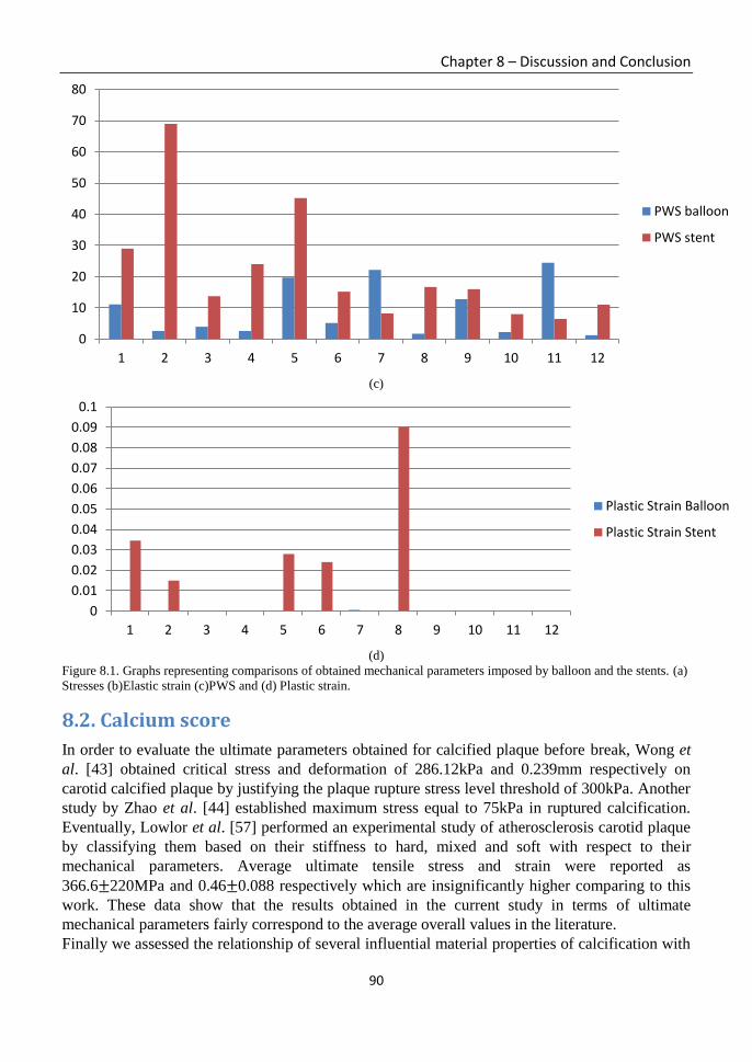
Chapter 8 – Discussion and Conclusion
90
(c)
(d)
Figure 8.1. Graphs representing comparisons of obtained mechanical parameters imposed by balloon and the stents. (a)
Stresses (b)Elastic strain (c)PWS and (d) Plastic strain.
8.2. Calcium score
In order to evaluate the ultimate parameters obtained for calcified plaque before break, Wong et
al. [43] obtained critical stress and deformation of 286.12kPa and 0.239mm respectively on
carotid calcified plaque by justifying the plaque rupture stress level threshold of 300kPa. Another
study by Zhao et al. [44] established maximum stress equal to 75kPa in ruptured calcification.
Eventually, Lowlor et al. [57] performed an experimental study of atherosclerosis carotid plaque
by classifying them based on their stiffness to hard, mixed and soft with respect to their
mechanical parameters. Average ultimate tensile stress and strain were reported as
366.6±220MPa and 0.46±0.088 respectively which are insignificantly higher comparing to this
work. These data show that the results obtained in the current study in terms of ultimate
mechanical parameters fairly correspond to the average overall values in the literature.
Finally we assessed the relationship of several influential material properties of calcification with
0
10
20
30
40
50
60
70
80
1 2 3 4 5 6 7 8 9 10 11 12
PWS balloon
PWS stent
0
0.01
0.02
0.03
0.04
0.05
0.06
0.07
0.08
0.09
0.1
1 2 3 4 5 6 7 8 9 10 11 12
Plastic Strain Balloon
Plastic Strain Stent

Chapter 8 – Discussion and Conclusion
91
obtained ultimate mechanical stresses/strains in order to investigate which material characteristics
are extremely involved in “plaque vulnerability” and “plaque protrusion”.
As a potentially influential parameter, we investigated on correlation between Ca score and
ultimate stress/PWS/external load for stent expansion. Although as mentioned before, in spite of
EM that is calcification-specific, Ca score is calculated based on all the lesions inside the carotid
artery. Nonlinear correlation between Ca score and ultimate stress was 0.44 (p=0.057) followed
by PWS that was 0.38 (p=0.103) in which shows no significant correlation exists. Likewise, there
is no statistically significant correlation between ultimate external load and Ca score in both
balloon and stent expansion as shown in Table 8.1 despite EM that showed strong positive
relationship (Chapter 3). This is because in reality large calcifications with high Ca score could
act as a ductile elastic material and conversely, calcifications with small Ca score might behave
as hard brittle material, hence it is not trivial to classify the calcifications base on its Ca score.
Another robust reason is that there is an element of “weight” that plays a big role in construction
of Ca score in which calcifications with the same range of HU have the same weight in their Ca
score [38]. Scatterplot in Figure 8.2 shows week correlation between Ca score and ultimate stress
imposed by both balloon and stent before break. Although among the rare probe on Ca score,
Nandalur et al. [58] statistically found that carotid artery Ca score have clinically significant
relationship with degree of stenosis and other cardiovascular risk factor, although as shown in
Table 8.1 in terms of mechanical parameters we concluded that Ca score has minor impact on
plaque break comparing to EM. However we believe that calculating calcification-specific Ca
score instead of One-for-all value could strength the proportion. Although the abovementioned
element of “weight” still influences the final correlation.
Mechanical Parameters Average values Correlation with Ca score
Ultimate external force 2.32±1.16 MPa R=0.53; p=0.089
Ultimate Stress 171±145 kPa R=0.44; p=0.057
Plaque Wall Stress 64.3±63.3 kPa R=0.38; p=0.103
Elastic Strain 0.08±0.06 R= -0.66; p=0.012
Table 8.1. Mechanical parameters obtained from Stent simulation and their nonlinear spearman’s correlation with Ca
Score. (statistically significant threshold, p<0.05).
Figure 8.2. Scatter plot showing weak correlation of Ca score and ultimate stress of calcifications obtained for balloon
and stent simulations.

Chapter 8 – Discussion and Conclusion
92
In addition to the statistical values obtained above, here we also presented the graph of
comparison of real values of the Ca score and HU, Volume score and EM that will be analyzed in
the next sections. Figure 8.3 below shows the comparisons for only 12 cases and obviously
volume score and HU have direct relation with Ca score. However EM in this graph seems not in
the direct correlation for some cases which is totally normal and their statistical relationship has
already been explained in Chapter 7. Panel (a) only presents elastic modulus belonging to 12
cases in the order of higher Ca score to the lower CA score. As can be seen relatively the higher
Ca score has the case, the higher EM is assigned to that case. C1 and C2, C3 and C4 with the
higher Ca score the also have higher EM. Panel (b) shows the proportion of CA score and HU
which since they have been obtained through the same equation they have direct correlation. In
panel (c) the relation of Ca score and volume score is shown. Similar to HU, since volume score
is one of the elements to obtain the Ca score, hence they have positive and direct correlation.
Finally in panel (d) standardized values belonging to Ca score and EM are shown. As stated in
the latter paragraph, they have relatively direct correlation.
(a)
(b)
0
1
2
3
4
5
6
1 2 3 4 5 6 7 8 9 10 11 12
Yo
un
g's
Mo
du
lus
(MP
a)
Patient No.
Elastic Modulus
0
500
1000
1500
2000
2500
1 2 3 4 5 6 7 8 9 10 11 12
CA Score HU

Chapter 8 – Discussion and Conclusion
93
(c)
(d)
Figure 8.3. Comparisons of Ca score in correlation with Volume score, HU and elastic modulus. Panel (a) shows only
EM belongs to 12 cases, (b) proportion of Ca score and HU, (c)corralation between Ca score and volume score and
(d)shows standardized values for Ca score and EM for the sake of seeking the relations.
0
500
1000
1500
2000
2500
1 2 3 4 5 6 7 8 9 10 11 12
CA Score Volume Score
-1.5
-1
-0.5
0
0.5
1
1.5
2
2.5
3
3.5
1 2 3 4 5 6 7 8 9 10 11 12
Ca Std EM Std

Chapter 8 – Discussion and Conclusion
94
8.3. Area and Volume score
The most common criteria to define a “vulnerable plaque” is the thickness of fibrous and lesion
size. Maldonado et al. [59] investigated on cap thickness including calcification in HR-μCT
images and confirms 300kPa threshold for cap rupture that correlates it with plaque thickness.
Likewise Vengrenyuk et al. [60] mathematically proves that calcified plaques smaller than 65μm
can reach to an ultimate stress of more than 600kPa. We investigated on correlation between area
of calcification and ultimate stress as well as PWS on stent expansion. The Spearman’s
coefficient was 0.43 (p=0.061) for ultimate stress and 0.39 (p=0.093) for PWS respectively, thus
the correlations are statistically not significant. The same relationship exists for volume score,
therefore size of calcification is not related to its fracture in the current study. This is because we
defined the rupture as the initial failure not the ultimate failure and since stress distribution is
function of both geometry and mechanical properties of the tissues, thus soon as indentation or
protrusion is met between contacts, stress distribution begins to occur leading to plaque
susceptibility. We also evaluated the proportion of area of calcification and ultimate external load
to know if the size has any impact on external load at break. We obtained spearman’s rho equal to
0.6 (p=0.008) that proves the larger the calcified plaque is, the higher load is required to press it.
8.4. Penetration and protrusion
Next, we evaluated penetration values obtained during stent expansion to figure out if any
correlation exists between EM and amount of protrusion in the calcified plaque. Spearman’s
correlation coefficient between EM and penetration was -0.9 (p<0.0001) considering as a strong
negative relationship. Therefore, the stiffer the calcification, the less protrusion occurs during the
expansion in CAS placement.
8.5. Ultimate External Pressure
Correlation of external loads and UTS/WSS/EM has already been presented in Sections III.B, C
for both balloon and stent expansion in which obviously shows a strong positive relationships.
However there is no statistically significant correlation between ultimate external load and Ca
score in both balloon and stent expansion by achieving spearman’s rho equal to 0.4 (p<0.084)
and 0.53 (p<0.019) respectively despite having strong correlation with EM. We also evaluated
the proportion of ultimate external load and area of calcification to know if the size has any
impact on external load at break time. We obtained spearman’s rho equal to 0.6 (p<0.008) that
proves the larger the calcified plaque is, the higher load is required to press it.
8.6. Tangent Modulus
Finally we examined the relationship exists between the numerically obtained TM that expresses
the amount of plasticity and EM as elastic property of calcifications in both balloon and stent
simulations. However in the balloon simulation due to some cases with zero TM, obtaining a
meaningful correlation is not possible, but an implicit correlation is inferred that higher the EM,
the less plastic (steeper slope) is the calcification, thus it is stiffer. However interpretation of this
behavior cannot be fully determined. The same conclusion is achieved for stent simulation that is
proved by a strong positive Spearman’s correlation between EM and TM equal to 0.791
(p<0.0001). This means that the steeper the elastic line is, the plastic slope also elevates higher
and vice versa.
Chapter 8 – Discussion and Conclusion
95
8.7. Conclusion
There is a gap in investigating the contribution of calcification in carotid artery plaque
vulnerability during interventional carotid artery stenting operation. We performed nonlinear
static structural simulations using Finite Element Method for both balloon and stent angioplasty
in order to obtain mechanical parameters i.e. ultimate stress/strain, external load involved in
calcified plaque fracture. The results correspond to the literature and nonlinear correlation
between the mechanical and material parameters shows a negative correlation between Ca score
and plaque rupture; however a strong positive correlation exists between elastic modulus of the
calcifications and plaque vulnerability.
The long term goal of the current work is to exploit the latter correlations and perform regression
analysis in order to develop a platform for pre-operative CAS operation and plaque vulnerability
prediction by deploying material and mechanical characteristics of the objects involved.
There were some limitations and assumptions that we considered in this study as follows:
Non-geometrical shapes of calcified plaque and the artery cause both CAD and CAE
nontrivial, and it has a considerable impact on the final results.
Lack of material properties for atherosclerotic calcification due to small amount of robust
experimental analysis.
Restriction in providing elaborated material properties for the stent and balloon from the
vendor.
Hemodynamic effect of blood flow on the imposed configuration is neglected due to
complexity in analysis of computational fluid dynamics and nonlinear static structural
modeling.
Due to limited sample size statistical analysis could be considered less robust, however
regression analysis is considered as future work in order to be able to prospect the sample
size and also to predict the mechanical parameters.
Obtaining these parameters and relationships helps the researchers in developing a virtual
platform for a pre-operative CAS in the future in order to predict the calcified plaque rupture and
maximum external load to impose.

96
Bibliography 1. A.G. Hauss and M.J. Yaffe, “A categorical course in physics: technical aspects of breast
imaging”, 78th Scientific Assembly and Annual Meeting of RSNA, 1994.
2. J.S. Suri and R.M. Rangayyan, “Recent Advances in Breast Imaging Mammography and
Computer-Aided Diagnosis of Breast Cancer”, 1st edn. SPIE, 2006.
3. M. Anbar, C. Brown, L. Milescu, J. Babalola, et al. “The Potential of Dynamic Area
Telethermometry in Assessing Breast Cancer”, IEEE Engineering in Medicine and Biology
Magazine, Vol. 19, Issue: 3, pp. 58-62, 2000.
4. M. Anbar, L. Milescu, C. Brown, C. Carty, et al. “Diagnosis of Breast Cancer with Infrared
Dynamic Area Telethermometry (DAT)”, Proc. Engineering in Medicine and Biology
Society. Vol.2, pp.1215-1218, 2000.
5. R. Joro, AL. Lääperi, S. Soimakallio, R. Järvenpää, T. Kuukasjärvi, T. Toivonen et al.
“Dynamic infrared imaging in identification of breast cancer tissue with combined image
processing and frequency analysis”, Med Eng Technol. Vol. 32(4), pp. 325-35, 2008.
6. V. Agostini, S. Delsanto, M. Knaflitz and F. Molinari, “Communications Noise Estimation in
Infrared Image Sequences: A Tool for the Quantitative Evaluation of the Effectiveness of
Registration Algorithms”, IEEE Transaction on Biomedical Engineering, Vol. 55, No. 7, pp.
1917-1920, 2008.
7. S. Riyahi-Alam, M. Peroni, G. Baroni and M. Riboldi, “Regularization in deformable
registration of biomedical images based on divergence and curl operators”, Methods Inf. Med.
Vol. 53, pp. 21–28, 2014.
8. Y.L. Sant. “An image registration method for infrared measurements”, Quantitative InfraRed
Thermography. Vol. 2, No.2, pp. 207-222, 2005.
9. V. Agostini, S. Delsanto, F. Molinari and M. Knaflitz. “Evaluation of feature-based
registration in dynamic infrared imaging for breast cancer diagnosis”, Proc. IEEE Eng Med
Biol Soc. Vol. 1, pp. 953-956, 2006.
10. V. Agostini, M. Knaflitz and F. Molinari, “Motion Artifact Reduction in Breast Dynamic
Infrared Imaging”. IEEE Transaction on Biomedical Engineering, Vol. 56, No.3, pp. 903-906,
2009.
11. L. Ibanez, W Schroeder. L. Ng and J Cates. The ITK software guide. Insight Toolkit Kitware
Inc, 2003.
12. N. Scales, C. Herry and M. Frize. “Automated Image Segmentation for Breast Analysis using
Infrared Images”, Proc. IEEE Eng Med Biol Soc. Vol. 3, pp. 1737-40, 2004.
13. 3D Slicer. [Internet]. Available from http://www.slicer.org.
14. J. V. Hajnal and D. L.G. Hill, Medical Image Registration, CRC Press, pp. 46-50, 2001.
15. S. Klein, M. Staring and J. P. W. Pluim, “Evaluation of Optimization Methods for Nonrigid
Medical Image Registration using Mutual Information and B-Splines”, IEEE Transaction On
Image Processing, Vol. 16, pp. 2879-2890, 2007.
16. T. Guerrero, G. Zhang, T. Huang, K. Lin, “Intrathoracic tumour motion estimation from CT
imaging using the 3D optical flow method”, Physics in Medicine and Biology, Vol. 49, No.
17, Aug 2004.
17. D. Rueckert, L. I. Sonoda, C. Hayes, D. L. G. Hill, M. O. Leach, and D. J. Hawkes, “Nonrigid
registration using free-form deformations”, Application to breast MR images, IEEE
Transaction on Medical Imaging, Vol. 18, No. 8, Aug 1999.
18. P. Viola, W. M. Wells, “Alignment by Maximization of Mutual Information”, International
Journal of Computer Vision, Vol. 24, Issue. 2, pp. 137–154, 1997.

97
19. G. E. Christensen, H. J. Johnson, “Consistent Image Registration”, IEEE Transaction on
Medical Imaging, Vol. 20, Issue. 7, pp.568 – 582, Aug 2002.
20. G. E. Christensen, J. He, “Consistent Nonlinear Elastic Image Registration”, IEEE
Transaction on Mathematical Methods in Biomedical Image Analysis, pp.37 – 43, Aug 2002.
21. T. Rohlfing, R. Calvin, Jr. Maurer, A. David, M. A. Jacobs, “Volume-Preserving Nonrigid
Registration of MR Breast Images Using Free-Form Deformation With an Incompressibility
Constraint”, IEEE Transaction on Medical Imaging, Vol. 22, Issue. 6, pp.730 – 741, July
2003.
22. Ch. Venkateswara Rao, K. M. M. Rao, A. S. Manjunath, and R. V. N. Srinivas. “Optimization
of automatic image registration algorithms and characterization”, Proceedings of the ISPRS
Congress, Istanbul, Turkey, pp. 698–702, July 2004.
23. H. Rezaei, S. Azadi, “Nonrigid Medical Image Registration using Hierarchical Particle Swarm
Optimization”, IEEE Transaction on Soft Computing, Computing with Words and Perceptions
in System Analysis, Decision and Control, ISBN: 978-1-4244-3429-9, pp. 1-4, Sep 2009.
24. A. Carreras, C. Ó. S. Sorzano, R. Marabini, J. M. Carazo, C. O. Solorzano, J. Kybic,
“Consistent and elastic registration of histological sections using vector-spline regularization,
in Computer Vision Approaches to Medical Image Analysis”, Lecture Notes in Computer
Science, Vol. 4241. Springer Berlin / Heidelberg, pp. 85-95, May 2006.
25. M. Chu, H. Chen, C. Hsieh, T. Lin, H. Hsiao, G. Liao, Qi Peng, “Adaptive Grid Generation
Based Non-rigid Image Registration using Mutual Information for Breast MRI”, Journal of
signal processing systems, Vol. 54, No. 1-3, pp. 45-63.
26. Akinlar, M. Ali, “A new method for non-rigid registration of 3D images”, PhD Dissertation,
University of Texas Arlington, DISS-10194, Jan 2009.
27. D. Ruan, S. Esedoglu, J. A. Fessler, “Discriminative sliding preserving regularization in
medical image registration”, IEEE International Symposium on Biomedical Imaging, Vol.
129, ISBN: 9781424439317, pp. 430-433, 2009.
28. M. Urschler, S. Kluckner, H. Bischof, “A Framework for Comparison and Evaluation of
Nonlinear Intra-Subject Image Registration Algorithms”, Institute of Computer Graphics and
Vision, Graz, University of Technology, Austria, Insight Journal, 2008.
29. P. Hellier, C. Barillot, I. orouge, B. Gibaud, G. Le Goualher, D. L. Collins, A. Evans, G.
Malandain, N. Ayache, G. E. Christensen, and H. J. Johnson, “Retrospective Evaluation of
Intersubject Brain Registration”, IEEE Transaction on Medical Imaging, Vol. 22, Issue. 9, pp.
1120 - 1130, Sep 2003.
30. A. Klein et al, “Evaluation of 14 nonlinear deformation algorithms applied to human brain
MRI registration”, Elsevier Science Direct Publication, NeuroImage, Vol. 46, Issue 3, pp.
786-802, July 2009.
31. T. Vercauteren, X. Pennec, et al. “Non-parametric diffeomorphic image registration with the
demons algorithm”, Proc. MICCAI. Vol. 10, pp. 319-326, 2007.
32. G. E. Christensen and H. J. Johnson, “Consistent Image Registration”, IEEE Transaction on
Medical Imaging, Vol. 20, Issue. 7, pp. 568-582, 2002.
33. T.M. Button, H. Li, P. Fisher, R. Rosenblatt, K. Dulaimy, S. Li et al. “Dynamic infrared
imaging for the detection of malignancy”, Phys. Med. Biol. Vol. 49, pp. 3105–3116, 2004.
34. G. E. Christensen, “Consistent Linear-Elastic Transformations for Image Matching”,
Information Processing In Medical Imaging, LNCS 1613, pp. 224-237, 1999.
35. H. Huang, R. Virmani, H. Younis, A.P. Burke, R.D. Kamm, R.T. Lee. “The impact of
calcification on the biomechanical stability of atherosclerotic plaques”. Circulation. Vol. 103,
Issue 8, pp. 1051–1056, 2001.

98
36. N. El-Barghouty, A. Nicolaides, V. Bahal, G. Geroulakos, A. Androulakis. “The identification
of the high risk carotid plaque”. European Journal of Vascular and Endovascular Surgery,
Vol. 11, Issue 4, pp. 470–478, 1996.
37. P. Tracqui, A. Broisat, J. Toczek, N. Mesnier, J. Ohayon, L. Riou. “Mapping elasticity moduli
of atherosclerotic plaque in situ via atomic force microscopy”. J Struct Biol, Vol. 174, Issue 1,
pp. 115–123, 2011.
38. Z. Teng, D. Tang, J. Zheng, P.K. Woodard, A.H. Hoffman. “An Experimental Study on the
Ultimate Strength of the Adventitia and Media of Human Atherosclerotic Carotid Arteries in
Circumferential and Axial Directions”. J Biomech, Vol. 42, Issue 15, pp. 2535–2539, 2009.
39. D. Bluestein, Y. Alemu, I. Avrahami, M. Gharib, K. Dumont, J.J. Ricotta, S. Einav.
“Influence of microcalcifications on vulnerable plaque mechanics using FSI modeling”. J
Biomech, Vol. 41, Issue 5, pp. 1111–1118, 2008.
40. D.I. Moussa, T. Rundek, J.P. Mohr, “Asymptomatic Carotid Artery Stenosis: A Primer on
Risk Stratification and Management”, 1st ed., CRC Press, 2007, pp. 22–24.
41. J.J. Mulvihill, M.T. Walsh. “On the mechanical behavior of carotid artery plaques: the
influence of curve-fitting experimental data on numerical model results”. Biomech Model
Mechanobiol, Vol. 12, Issue 5, pp. 975–985, 2013.
42. G.A. Holzapfel, J.J. Mulvihill, E.M. Cunnane, M.T. Walsh. “Computational approaches for
analyzing the mechanics of atherosclerotic plaques: a review”. J Biomech, Vol. 47, Issue 4,
pp. 859–869. 2014
43. K.K. Wong, P. Thavornpattanapong, S.C. Cheung, Z. Sun, J. Tu. “Effect of calcification on
the mechanical stability of plaque based on a three-dimensional carotid bifurcation model”.
BMC Cardiovasc Disord, 12:7, 2012.
44. S. Zhao, L. Gu, S. R. Froemming. “Finite element analysis of the implantation of a self-
expanding stent: impact of lesion calcification”. Journal of Medical Devices, Vol. 6, Issue 2,
pp. 021001, 2012.
45. C. Yang, G. Canton, C. Yuan, M. Ferguson, T.S. Hatsukami, D. Tang. “Advanced human
carotid plaque progression correlates positively with flow shear stress using follow-up scan
data: an in vivo MRI multi-patient 3D FSI study”. J Biomech, Vol. 43, Issue 13, pp. 2530–
2538, 2010.
46. T. Miura, N. Matsukawa, K. Sakurai, H. Katano, Y. Ueki, K. Okita, K. Yamada, K. Ojika.
“Plaque vulnerability in internal carotid arteries with positive remodeling”. Cerebrovasc Dis
Extra, Vol. 1, Issue 1, pp. 54–65, 2011.
47. A. Agatston, W.R. Janowiz, F.J. Hildner, N.R. Zusmer, M. Jr. Viamonte, R. Detrano.
“Quantification of coronary artery calcium using ultrafast computed tomography”. J Am Coll
Cardiol. Vol. 15, Issue 4, pp. 827–832, 1990.
48. H.E. Boyer, “Atlas of Stress-strain Curves”, 2nd ed., ASM International, pp. 12–17, 2002.
49. M.A. Meyers, P.Y Chen, “Biological Materials Science: Biological Materials, Bioinspired
Materials, and Biomaterials”, 1st ed., Cambridge University Press, pp. 237–245, 2014.
50. L.L. Demer, Y. Tintut. “Vascular calcification: pathobiology of a multifaceted disease”.
Circulation, Vol. 117, Issue 22, pp. 2938–2948, 2008.
51. C.L. Higgins, S.A. Marvel, J.D. Morrisett. “Quantification of calcification in atherosclerotic
lesions”. Arterioscler Thromb Vasc Biol., Vol. 25, Issue 8, pp. 1567-1576, 2005.
52. J.Y. Rho, M.C. Hobatho, R.B. Ashman. “Relations of mechanical properties to density and
CT numbers in human bone”. Med. Eng. Phys., Vol. 17, Issue 5, pp. 347-355, 1995.
53. U. Schneider, E. Pedroni, A. Lomax. “The calibration of CT Hounsfield units for radiotherapy
treatment planning”. Phys Med Biol., Vol. 41, Issue 1, pp. 111-124, 1996.
99
54. R. Molteni, “From CT Numbers to Hounsfield Units in Cone Beam Volumetric Imaging: the
effect of artifacts” 62th AAOMR, Annual Session, Chicago Illinois., (8-11), Dec. 2011.
55. E. Maher, A. Creane, S. Sultan, N. Hynes, C. Lally, D.J. Kelly. “Tensile and compressive
properties of fresh human carotid atherosclerotic plaques”. J Biomech., 42(16), pp. 2760-
2767, 2009.
56. R.T. Lee, S.G. Richardson, H.M. Loree, A.J. Grodzinsky, S.A. Gharib, F.J. Schoen, N.
Pandian. “Prediction of mechanical properties of human atherosclerotic tissue by high-
frequency intravascular ultrasound imaging an in vitro study”. Arteriosclerosis, Thrombosis
and Vascular Biology, Vol 12, Issue 1, pp. 1-5, 1992.
57. M.G. Lawlor, M.R. O'Donnell, B.M. O'Connell, M.T. Walsh. “Experimental determination of
circumferential properties of fresh carotid artery plaques”. J Biomech., Vol. 44, Issue 9, pp.
1709-1715, 2011.
58. K.R. Nandalur, E. Baskurt, K.D. Hagspiel, M. Finch, C.D. Phillips, S.R. Bollampally, C.M.
Kramer. “Carotid artery calcification on CT may independently predict stroke risk”. AJR Am
J Roentgenol., 186(2), pp. 547-552, 2006.
59. N. Maldonado, A. Kelly-Arnold, Y. Vengrenyuk, D. Laudier, J.T. Fallon, R. Virmani, L.
Cardoso, S. Weinbaum. “A mechanistic analysis of the role of microcalcifications in
atherosclerotic plaque stability: potential implications for plaque rupture”. Am J Physiol Heart
Circ Physiol., Vol. 303, Issue 5, pp. 619-628, 2012.
60. Y. Vengrenyuk, S. Carlier, S. Xanthos, L. Cardoso, P. Ganatos, R. Virmani, S. Einav, L.
Gilchrist, S. Weinbaum. “A hypothesis for vulnerable plaque rupture due to stress-induced
debonding around cellular microcalcifications in thin fibrous caps”. Proc Natl Acad Sci U S
A., 103(40), pp. 14678-14683, 2006.

100
Curriculum Vitae

101
PERSONAL INFORMATION
Sadegh Riyahi Alam
Address: Corso Duca degli Abruzzi, n. 24, Department of Mechanical and Aerospace engineering, Politecnico di Torino, 10129, Turin, Italy. Office phone: +39-(0)11-903394, Mobile: +39-3284563145
Email: [email protected]
Skype ID: sadeghit
Website: http://socrate.polito.it/biolab/Home.html
Researchgate: https://www.researchgate.net/profile/Sadegh_Riyahi_Alam
Linkedin: https://www.linkedin.com/profile/public-profile-settings?trk=prof-edit-edit-public_profile
Date of birth: 17/01/1983 | Nationality: Iranian
RESEARCH INTERESTS
Computer aided detection/diagnosis (CAD), Computer Vision.
Medical image processing, Image Registration and Segmentation.
Biomechanical finite element analysis (FEM), CAD/CAE.
Cardiovascular imaging, Vascular mechanobiology, Carotid Artery Stenting, Atherosclerosis.
Breast dynamic infrared imaging, Digital Mammography.
4DCT Adaptive/Image guided radiotherapy.
EDUCATION
Jan 2012 – Jan 2015 PhD in Biomedical Engineering
Politecnico di Torino, Turin, Italy
Thesis title: Preoperative Systems for Computer-Aided-Diagnosis based on
image registration: applications to Breast Cancer and Atherosclerosis.
I have been involved in two projects to develop a Computer Aided Diagnostic System comprising: 1. Implementation of automated 3D time-series image registration methods
in Breast Dynamic Infrared Images for detection of breast cancer. We developed both linear and non-linear registration methods using ITK in order to remove the patient movements to facilitate the patient acquisition procedure and improve further spectral analysis of vascular temperature modulation for the prospective breast cancer prognosis.
2. Patient-specific pre-operative carotid artery stenting simulation using Finite
Element Analysis by considering Agatston score of calcified plaques in which using Computer Vision and in silico analysis, we assessed contribution of calcification in carotid atherosclerotic plaque rupture. We also performed correlation/regression analysis between material properties of calcification and obtained mechanical parameters to predict the plaque vulnerability.

102
RESEARCH EXPERIENCES
Feb 2009 – Dec 2011 Master of Science in Computer Engineering
Politecnico di Milano, Milan, Italy
▪ Thesis title: Implementation of divergence and curl operators embedded cost
function in deformable image registration for adaptive radiotherapy.
Sep 2001 – Sep 2006
Bachelor of Science in Computer Engineering (Software)
Azad University-Tehran Central Branch, Tehran, Iran
▪ Thesis title: Mammographic reporting and viewer software developed for
Computer Aided Diagnostic (CAD) system of screening mammography.
Oct 2013 – May 2014 Visiting researcher in vascular mechanobiology
Yokoyama Lab, Department of Biomedical Engineering, Nagoya city university, Nagoya, Japan.
Department of Neurosurgery, Nagoya City University Graduate School of Medical Sciences, Nagoya, Japan.
Supervisors: Kiyoko Yokoyama, Hiroyuki Katano
▪ Computer vision based nonlinear static simulation of patient-specific pre-operative carotid artery stenting using in vivo MDCT images in order to evaluate mechanical and material behaviour of calcified plaques in plaque vulnerability by exploiting finite element method.
Sep 2010 – Dec 2011 Trainee in biomedical image processing
TBM Bioengineering Laboratory Technologies, Department of Bioengineering, Politecnico di Milano, Milan, Italy.
Supervisors: Marco Riboldi, Marta Peroni, Guido Baroni
▪ Analyse and implementation of a novel cost function for deformable image registration of 4DCT images using divergence and curl operators for adaptive radiotherapy application by ITK, VTK and Plastimatch.
July 2005 – Feb 2009
Image processing software developer
Medal Electronic Engineering Co. Ltd., Tehran, Iran. http://www.medalelectronic.com
Supervisor: R. Aghazadeh Zoroufi
▪ Implementation of a Computer Aided Diagnostic System for microcalcification and mass detection in digital xray mammograms.
▪ Development of a Computer Aided Diagnostic Software for segmentation of Multiple Sclerosis (MS) plaques in MRI images using 3D slicer, FSL and MRIcron.
103
PUBLICATIONS
International Journals
1. S. Riyahi-Alam, K. Yokoyama, H. Katano, U. Morbiducci, A. Audenino, F.
Molinari, “Preoperative carotid artery stenting simulation using Finite Element
Analysis by considering Agatston score of calcified plaques”, IEEE transaction on
Biomedical Engineering, Submitted Feb 2015. In Peer-review.
2. S. Riyahi-Alam, V. Agostini, F. Molinari, M. Knaflitz, “Comparison of time-
series registration methods in breast dynamic infrared imaging”, Journal of Opto-
Electronics Review, ISSN:1230-3402; Vol 23, Issue 1, January 2015, pp.68-77.
3. S. Riyahi-Alam, M. Peroni, G. Baroni, M. Riboldi. “Regularization in
deformable registration of biomedical images based on divergence and curl
operators”, Journal of Methods of Information in Medicine, ISSN: 0026-1270; Vol
53, Issue 1, January 2014, pp.21-28.
4. S. Riyahi-Alam, N. Riahi. “Implementation analysis of a Mammographic
Computer-Aided Diagnostic (CAD) System”, International Journal of Medical
Physics, Vol 38, Issue 6, 3396 / Joint AAPM/COMP Meeting Program, July 2011.
5. N. Riahi, F. Younesi, S. Riyahi-Alam. “Computer-Aided Mass Detection on
Digitized Mammograms using a Novel Hybrid Segmentation System”, North
Atlantic University Union (NAUN) International Journal Of Biology And
Biomedical Engineering, Vol 3, Issue 4, 2009, pp.51-56.
Conference roceedingsP
1. S. Riyahi-Alam, U. Morbiducci, H. Katano, K. Yokoyama, S. Ali, A. Audenino,
F. Molinari, “Preoperative in silico analysis of atherosclerotic calcification
vulnerability in carotid artery stenting using Finite Element Analysis by
considering Agatston score”, World Congress on Medical Phys. and Biomedical
Eng–IFMBE / IUPESM 2015, Jun 2015, Toronto, Canada, Submitted, In Peer
Review.
2. S. Ali, M. Giachino, A. Bonani, A. Aprato, S. Riyahi-Alam, A. Khattab, C.
Bignardi, A. Massè, “Pelvic Ring Fractures: External Fixation Comparative
Numerical Structural Analysis”, Proceeding of IEEE 7th Cairo International
Biomedical Engineering Conference-IBEC2014, Dec 2014, Giza, Egypt.
3. S. Riyahi-Alam, V. Agostini, F. Molinari, M. Knaflitz. “Evaluation of time-series
registration methods in Dynamic Area Telethermometry for breast cancer
detection”, Proceeding of 12th International Conference on Advanced Infrared
Technology and Applications, Sep 2013, Turin, Italy, pp. 147-159.
TECHNICAL SKILLS - Excellent programming skills in MATLAB and Visual C++ using ITK, VTK. - Experienced in 3D Slicer, Amira, Plastimatch, FSL, MRIcron and PACSPLUS
for CT and MRI data analyses. - Good knowledge in Finite Element Method and CAD/CAE using Mimics, Rhinoceros, Solidworks and Ansys. - Good knowledge in Statistical software Minitab as well as Unix and Linux operating systems. - Good programming skills in ADO and ODBC database technology with Microsoft SQL Server.
PROFESSIONAL ACTIVITY
Reviewer: Journal of Medical Imaging and Health Informatics (JMIHI). Workshop: 1
st International workshop on Nanotechnology in Cancer Treatment.
10th
Nov 2014. Castello del Valentino, Politecnico di Torino.

104
AWARDS and SCHOLARSHIPS
1. The best paper award: 12th International Conference on Advanced Infrared
Technology and Applications (AITA 2013), Castello Del Valentino, Turin, Italy, Sep 2013.
2. The Italian Government: Italian Government Scholarship. 2012-2015.
3. Award: Innovations, Inventions and Scientific Speculation for “Designing a Computer-Aided-Diagnostic System (CAD) for Assessment of Digital Mammograms in Iran”, The 11th Razi Research Festival on Medical Sciences, Ministry of Health &
Higher Medical Educations, 27th December, 2005, Tehran, Iran.
REFERENCES Prof. Filippo Molinari, Associate professor at department of Electronics and Telecommunication, Politecnico di Torino, Turin, Italy. Website: http://socrate.polito.it/biolab/Home.html. Email: [email protected]. Tel: +39 (0)110904135
Prof. Kiyoko Yokoyama, Professor at Graduate School of Design and Architecture, Nagoya City University, Nagoya, Japan. Website: http://www.sda.nagoya-cu.ac.jp/yokoyama. Email: [email protected]. Tel: +81-52-721-5439
Prof. Alberto Audenino, Professor at department of Mechanical and Aerospace engineering, Politecnico di Torino, Turin, Italy.
Email: [email protected]. Tel: +39 (0)110906932
BACKGROUND SUMMARY
Graduating in biomedical engineering, I have deep technical skills in software development, specially in computer aided diagnostic/detection systems for biomedical applications. Starting from my academic career I was involved in several projects such as mass and microcalcification detection in digital mammography and implementation of novel deformable image registration for adaptive radiotherapy applications. During my PhD career, as a visiting researcher in Nagoya university, I was involved in biomechanical project of patient-specific pre-operative carotid artery stenting simulation using Finite Element Analysis in which elastic-plastic material behaviour of the calcification is observed in Atherosclerotic plaque rupture. I also carried out a project regarding image/signal processing for implementation of 3D Time-series registration methods on dynamic infrared images for breast cancer detection to facilitate the spectral analysis of vascular temperature modulation for further prognosis. In these projects I was able to deal with complex and multi-disciplinary subjects both in individual and team work with high level of autonomy.
PERSONAL SKILLS
Mother tongue(s) Persian
Other language(s) UNDERSTANDING SPEAKING WRITING
Listening Reading Spoken
interaction Spoken
production
English C1 C1 C1 C1 C2
Japanese C1 C1 C1 C1 C1
Italian B1 B1 B1 B1 B1
Levels: A1/2: Basic user - B1/2: Independent user - C1/2 Proficient user

105
Publications

106
1. S. Riyahi-Alam, K. Yokoyama, H. Katano, U. Morbiducci, A. Audenino, F. Molinari,
“Preoperative carotid artery stenting simulation using Finite Element Analysis by considering
Agatston score of calcified plaques”, IEEE transaction on Biomedical Engineering, Submitted Feb
2015. In Peer-review.
2. S.Riyahi-Alam, V. Agostini, F. Molinari, M. Knaflitz, “Comparison of time-series registration
methods in breast dynamic infrared imaging”, Journal of Opto-Electronics Review, ISSN:1230-
3402; Vol 23, Issue 1, January 2015, pp.68-77.
3. S.Riyahi-Alam, M. Peroni, G. Baroni, M. Riboldi. “Regularization in deformable registration of
biomedical images based on divergence and curl operators”, Journal of Methods of Information in
Medicine, ISSN: 0026-1270; Vol 53, Issue 1, January 2014, pp.21-28.
4. S. Riyahi-Alam, N. Riahi. “Implementation analysis of a Mammographic Computer-Aided
Diagnostic (CAD) System”, International Journal of Medical Physics, Vol 38, Issue 6, 3396 / Joint
AAPM/COMP Meeting Program, July 2011.
5. N. Riahi, F. Younesi, S. Riyahi-Alam. “Computer-Aided Mass Detection on Digitized
Mammograms using a Novel Hybrid Segmentation System”, North Atlantic University
Union (NAUN) International Journal Of Biology And Biomedical Engineering, Vol 3, Issue
4, 2009, pp.51-56.
6. S.Riyahi-Alam, U. Morbiducci, H. Katano, K. Yokoyama, S. Ali, A. Audenino, F. Molinari,
“Preoperative in silico analysis of atherosclerotic calcification vulnerability in carotid artery
stenting using Finite Element Analysis by considering Agatston score”, World Congress on
Medical Phys. and Biomedical Eng–IFMBE / IUPESM 2015, Jun 2015, Toronto, Canada,
Submitted, In Peer Review.
7. S. Ali, M. Giachino, A. Bonani, A. Aprato, S.Riyahi-Alam, A. Khattab, C. Bignardi, A. Massè,
“Pelvic Ring Fractures: External Fixation Comparative Numerical Structural Analysis”,
Proceeding of IEEE 7th Cairo International Biomedical Engineering Conference-IBEC2014, Dec
2014, Giza, Egypt.
8. S. Riyahi-Alam, V. Agostini, F. Molinari, M. Knaflitz. “Evaluation of time-series registration
methods in Dynamic Area Telethermometry for breast cancer detection”, Proceeding of 12th
International Conference on Advanced Infrared Technology and Applications, Sep 2013, Turin,
Italy, pp. 147-159.