Policy Uncertainty, Multinational Firms, and Reallocation ∗

Arkodipta Sarkar†

December 26, 2019

Job Market Paper

Abstract

Multinationals are often considered a tool through which economic shocks originat-

ing in a region get magnified. This paper, in contrast, shows that elevated economic

policy uncertainty (EPU) in a country is associated with increase in investment by a

firm in other regions. I find that (multinational) firms hold back investment in a coun-

try subjected to higher EPU, which they reallocate to projects in other countries. I

find the impact to be higher for firms with tighter financial constraints. I also find that

the reallocation is directed more towards countries that provide a better legal environ-

ment. The study uses establishment-level data of mining firms as a laboratory. Limited

input–output linkage across mines allows me to study the impact caused particularly

through the allocation decision of firms. The empirical strategy exploits variations in:

i) parent country of mines operating in the same country; & ii) country of operation

of mines owned by same firm. Overall, my findings highlight that multinationals could

potentially stabilize the escalation of regional policy uncertainty shocks to global crisis.

∗I wish to thank the AQR Asset Management Institute and the Wheeler Institute at London BusinessSchool for their financial support. I am extremely grateful to my advisor Vikrant Vig for his invaluableguidance and support. I thank Pat Akey, Aleksander A. Aleszczyk, Simcha Barkai, Bo Bian, LorenzoBretscher, Svetlana Bryzgalova, Joao Cocco, Ian Cooper, Nuno Clara, Mahitosh Dutta, Dimas MateusFazio, Raymond Fisman, Julian Franks, Francisco Gomes, Marco Grotteria, Denis Gromb, Thilo Kind,Howard Kung, Stefan Lewellen, Lakshmi Sankararama Naraayanan, Narayan Naik, Elias Papaioannou, AnnaPavlova, Ashish Sahay, Ishita Sen, Henri Servaes, Gunjan Seth, Rui Silva, Manpreet Singh, Varun Sharma,Shikhar Singla, Janis Skrastins, Prasanna Tantri, Gareth Taylor, Philip Woodhead and all participants atthe London Business School internal seminar, Trans-Atlantic Doctoral Conference (TADC), LBS AlumniWorkshop 2019 and HEC Paris finance PhD workshop 2019.†London Business School, e-mail: asarkar@london.edu

1 Introduction

Since the financial crisis in the US, there has been an increased interest in studying the

link between policy-related uncertainty and economic outcomes in general and firms’ decision

making in particular (Baker, Bloom, and Davis (2016), Julio and Yook (2012), among others).

A significant proportion of firms (particularly in developed countries) are multinational in

nature and represent a primary feature of the world economy through which shocks tend

to propagate (Alviarez (2019)). Cravino and Levchenko (2016) estimates that 20–40% of a

foreign affiliate’s shock has its origin in their home country. Given this premise, this paper

studies the way multinational firms, through their decision to allocate resources, propagate

policy-related uncertainty across countries.

There is a growing body of research that studies the way economic shocks originating

in a country could have a negative impact on other economies. Multinational firms have

been particularly highlighted as a tool through which local shock can magnify and thereby

escalate to global crisis. This is empirically observed through a negative shock to funding or

business cycle fluctuations at the parent firm location and a consequent reduction in economic

activity across foreign affiliates (Desai and Foley (2004), Cravino and Levchenko (2016),

Alviarez (2019), Biermann and Huber (2019), among others). Economic policy uncertainty

(henceforth, EPU), causing reductions in the economic activity of firms, manifests itself as

a negative shock like any other. Consequently, it is natural to expect that a rise in EPU is

also likely to be negatively propagated across countries through multinational firms. This

paper, in contrast, finds that an increase in EPU in a country is associated with an increase

in investment by a multinational firm in their foreign operations. I find that firms reduce

investment in the location with elevated EPU and are left with additional resources that

they can internally allocate to other business units, thereby causing a positive propagation.

This paper, consequently, provides evidence of an instance whereby multinational firms could

prevent the escalation of local shock to global crisis.

There are several challenges that might hinder the empirical identification of a multina-

tional firm’s allocation decision across countries caused by economic policy uncertainty. To

fix idea, consider a period of elevated policy uncertainty caused by the discussion around

possible reduction in government budget deficit in a country (say Canada). The first concern

is that the uncertainty in Canada could itself lead to overall attractiveness to invest in a

competing country that has a more stable policy outlook (say Australia), creating an in-

crease in aggregate demand there. Alternatively, this period of uncertainty in Canada could

be correlated with local economic factors in Australia. Secondly, uncertainty in Canada

1

could lead to reduction in production of engines by a manufacturing firm (say Bombardier)

in Canada which might cause a reduction in investment in Bombardier’s assembling unit in

Thailand. However, this could be owing to engines being an input in assembling segment

and not necessarily through the allocation decision of the firms.

Using a laboratory of mining sector firms, I address the first concern by comparing op-

erations of Canadian multinational mining firms in Australia with other mining operations

there, and consequently subjected to the same local conditions. This also allows me to high-

light the importance of multinational firms’ ability to flexibly allocate capital and labour

across different operations. Using mining firms with limited production linkages as my em-

pirical setup also allows me to particularly identify internal capital decision making from

production linkages across different units of the same firm.

The empirical analysis of this paper uses database on international operations of mining

firms domiciled in multiple countries and data on economic policy uncertainty index of 15

countries constructed by Baker, Bloom, and Davis (2016). This allows me to infer whether

a mine is facing policy uncertainty in its home country.1 Therefore, I can compare the

difference in investment of firms mining in the same country (and in most instances, mining

the same commodity) but subject to periods of varying degrees of EPU in their respective

home countries. Multinational firms hold back investment in the country with elevated

policy uncertainty and internally reallocate it to projects in other countries that are in need

of capital. This provides a basis to investigate cross-sectional heterogeneity based on the

degree of financial constraint to which a firm is subjected. Next, I investigate whether the

institutional quality, measured as bilateral investment treaty (BITs) between two countries

plays a role in firms’ choice of the location of investment during periods of elevated economic

policy uncertainty. Finally, since I know the location of mining properties, I use satellite

images of light density at night around the mines as a credible measure of local growth to

quantify the positive effect of foreign uncertainty in economic activity.

The analysis in this paper begins by looking at the share of capital expenditure (capex) of

mining firms that move to a foreign economy when a country is subject to periods of elevated

EPU. I find that a 100% increase in EPU in a country is associated with a 10 percentage

point increase in the share of expenditure in foreign countries by the multinationals. It is

associated with decrease in capex by firms in the domestic country and an increase in the

foreign countries, while the aggregate firm level capex remains largely unchanged. The results

indicate that multinationals shift investment to other countries in response to domestic EPU

1Alternatively, I also use uncertain elections as a measure of periods when economic policy uncertaintyis particularly high.

2

and thereby prevent local shocks from magnifying globally.

As discussed above, the result could, however, be driven by investment opportunities in

foreign countries and not by the rising EPU in the country of firm. To rule these concerns

out, I look at capex in a country (thereby subject to the same local conditions) by firms

with varying countries of origin. I find that as EPU in the country of headquarters of the

firm doubles (increases by 100%), capex increases by around 23%. To put this magnitude

in perspective, the EPU index rises on average by around 25% in the year of imminent

elections, leading to around a 6% increase in expenditure in foreign countries. On looking

at within-firm allocation (including firm × year fixed effect), I find the magnitude to rise

sharply, highlighting internal reallocation of resources across countries.

Next, I compare investment in establishments in the same country, mining the same com-

modity, but owned by firms varying in their country of origin. I find that the ratio of

investment to value of mines increases by 20 basis points in foreign mines as the policy

uncertainty index in their home country doubles. Given that the mean is around 90 basis

points, the result shows an increase by more than 20%. These pieces of evidence taken to-

gether highlight that multinational firms tend to reallocate investment outside as domestic

EPU increases.

To further probe the underlying mechanism behind the empirical findings, I exploit several

dimensions of heterogeneity in the data. I begin by examining the differential effect of

EPU on investment in the foreign establishment of firms varying in their degree of financial

constraints. As discussed before, the thesis in this paper builds on the idea that firms

withhold investment in the region that has high policy uncertainty and consequently are left

with resources that they can potentially allocate to establishments in other regions. If all

the unaffected business units of a firm are operating at their optimum without any financial

constraint, there might be no reallocation of investment by the multinational firm. Also,

the additional resource is more valuable to a firm that was subjected to a tighter constraint

and thereby slackens the constraint by a greater magnitude.2 The finding echoes Fazzari,

Hubbard, and Petersen (1988), where investment is shown to have greater sensitivity to cash

flow for financially constrained firms.

Next, I investigate whether institutional quality in the country where the mines are located

drives the intensity of reallocation. The idea is that better quality of institutions provides

2Since the optimality condition for a constrained firm requires that the marginal revenue product of capitaldeviate from its cost by the degree of financial constraint, greater reduction in the constraint is associated witha higher increase in investment under standard upward sloping concave production technology. Consistentwith this, I find the impact of foreign EPU to be higher in establishments of firms with stricter financialconstraints.

3

better protection for investors and hence such countries would be more attractive as invest-

ment destinations during periods of policy uncertainty.3 I use BITs signed by two countries

as a measure of institutional quality between the signatories (Bhagwat, Brogaard, and Julio

(2017), Cao, Li, and Liu (2017)). BITs particularly protect investors from expropriation risk

as well as allowing easier repatriation of profits. I find that firms shift their investment to

countries that provide better institutional quality. BITs allow me to compare investment

in mines in the same host country where institutional quality differs for different foreign

countries.4

I also explore alternate definitions of policy uncertainty and country of origin of a firm to

establish robustness of the results in this paper. Following the literature, I use three alternate

ways of identifying periods of elevated EPU. First, I use periods prior to elections in general

and close elections in particular as an alternate measure of policy uncertainty (Akey (2015),

Jens (2017), Asher and Novosad (2017), among others). Second, I use an uncertainty index

constructed by Ahir, Bloom, and Furceri (2018) which uses economic intelligence unit country

reports made by IMF. Third, I use the residual from regressing country EPU on global EPU

(Davis (2016)) as a measure of policy uncertainty for each country. The primary results of

the paper are qualitatively the same in all the above instances. The result is also robust to

alternate definition of home country as country where the maximum operations of the firms

are located. I also provide some external validity of the results using compustat segment

data and find that as EPU in the US increases, firms tend to shift investment in their foreign

subsidiaries.

There can be a possible concern that the results in the paper are driven by changes

in expectations and not necessarily by policy-related uncertainty. I attempt to address

this concern in the following way. Firstly, I include measures of sentiment indices in the

empirical analysis as a control for changes in expectation (Gulen and Ion (2015), Hassan,

Hollander, van Lent, and Tahoun (2019), among others). Secondly, I split my sample between

periods of relatively high and low sentiment with the idea that if the result is driven by

negative sentiment then the relationship between EPU and foreign investment should be

3Refer to Acemoglu, Johnson, and Robinson (2005) for a review of the role of institutional quality or thelack thereof as a potential cause of underdevelopment.

4The optimality condition of resource allocation would require the marginal revenue product per unitcost of capital to be equalized across all establishments, and for a constrained firm it equals the degree ofthe constraint. Since better institutional quality is associated with higher marginal productivity, it impliesgreater allocation of resources. As discussed before, elevated policy uncertainty frees up resources to allocatein other establishments. This implies that under the new optimality condition, the marginal revenue productof all the establishments has to decrease (i.e. increase in capital). The concavity of the function would requirea greater increase in capital for establishments which are already operating at a higher level of capital. Thiswould then manifest as more resources being allocated to establishments located in places that provide betterlegal institutions.

4

significant only in periods of negative sentiment. I find that that the relation between

EPU and investment in foreign countries is identical in either of the sample splits. Thirdly,

uncertain elections provide an event where uncertainty resolves after the election. I find

the effect on foreign investment fades immediately after the election as the uncertainty is

resolved. Meanwhile, I do not find any change during less uncertain elections. Expectations

are, however, likely to change during any elections.

In the final analysis of the paper, I investigate whether the allocation of investment to

foreign economies has a positive impact in the local economic activity around the mines.

For this purpose, I look at economic activity measured as night time light in arbitrarily

drawn small areas called cells of 55 × 55 km2 (0.5 × 0.5 degree latitude). The idea is

that reallocation of assets might not have an aggregate effect for the entire country, but the

positive spillover could occur at a local level around the mines. I map the mining properties

to each of the cells. Thus, for each cell I know whether it has a mine and if that mine is

owned by a domestic or foreign company. Also, for each of these cells I have night time

light data obtained from satellite images, which have been shown in the literature as a

good proxy for local economic activity. I find that the level of economic activity measured

by the luminosity data around foreign mines is 5% higher following a 100% increase in

policy uncertainty originating from their home countries, suggesting positive spillover in real

economic activity.5

In summary, I find that multinational firms tend to invest more in foreign countries as

a response to domestic policy uncertainty. The empirical strategy helps me to control for

investment opportunities coming up in foreign countries and other linkages that might drive

the result. I also attempt to indicate that the results are driven primarily by uncertainty

aspect of possible policy changes and not necessarily through changes in expectations. In

contrast to previous findings where multinationals have been considered a catalyst for shock

propagation across countries, I provide a scenario where multinational firms could act as a

global stabilizer and prevent local shocks from escalating to a global magnitude.

Related Literature: This research contributes most directly to the literature on the role

of policy uncertainty on firms’ decision making, and it extends it by studying the way policy

uncertainty propagates across countries. Julio and Yook (2012) and Jens (2015), among oth-

ers, used elections as a measure of policy uncertainty to show that firms decrease investment

during elections. Meanwhile, economic policy uncertainty index developed by Baker, Bloom,

and Davis (2016) has been used to study the impact of uncertainty surrounding policy deci-

5Meyer (2004) provides a review highlighting the need to better understand the role of multinationalenterprises in broader social and environmental contexts, particularly in developing countries.

5

sions on investment by firms, mergers and acquisitions, and other economic activity (Gulen

and Ion (2015), Akey and Lewellen (2015), Bonaime, Gulen, and Ion (2018)).6 I contribute

to this strand of literature by studying the way resources are allocated within a firm in the

face of policy uncertainty. This also allows me to contribute to the literature by examin-

ing how policy uncertainty in a country spills over to other economies. At a macro level,

Gauvin, McLoughlin, and Reinhardt (2014) and Kloßner and Sekkel (2014) show how un-

certainty related to macroeconomic policies propagates to other countries through portfolio

flows. Julio and Yook (2016) highlighted a drop in aggregate FDI flows from US companies

during periods of election activity in the host countries. Cao, Li, and Liu (2017) looks at

cross-border mergers and acquisitions during periods of national elections, while Campello,

Cortes, d’Almeida, and Kankanhalli (2018) highlights the way investment by US compa-

nies decreased following Brexit in the UK. The current paper is distinct from these existing

works in several different ways. First, I highlight the importance of firms operating in mul-

tiple countries in propagating uncertainty through their internal decision to invest across

different mines and thereby provide a a microeconomic understanding of policy uncertainty

that might spill over through reallocation of assets by firms with a global presence. Second,

the setting allows me to control for local economic shocks and identify the impact of policy

uncertainty from foreign economies. Third, the mining sector provides a setting wherein I

can distinguish internal capital decision making in propagation of policy uncertainty from

other production and input–output linkages.7 The granularity of the data also allows me to

control for several other confounding factors. Finally, my result highlights a scenario where

policy uncertainty can positively impact investment in foreign countries.

A growing literature highlights the way shocks tend to propagate in an economy: produc-

tion linkages (Acemoglu, Carvalho, Ozdaglar, and Tahbaz-Salehi (2012), Acemoglu, Akcigit,

and Kerr (2016), Barrot and Sauvagnat (2016), among others); financial and social linkages

(Acemoglu, Ozdaglar, and Tahbaz-Salehi (2015), Acemoglu, Ozdaglar, and Tahbaz-Salehi

(2015)); and international banking (Schnabl (2012), Gilje, Loutskina, and Strahan (2016)).8

Lamont (1997) shows that cash flow shock in the oil subsidiaries of a firm could lead to

reduction in capital expenditure of non-oil subsidiaries. This paper attempts to causally

infer the role of multinational firms and/or firms with multiple establishments in spreading

6There is also a large literature on the impact of policy or political uncertainty on asset prices Brogaardand Detzel (2015),Pastor and Pietro (2003), Pastor and Veronesi (2013).

7The mining sector has been used for empirical studies by Tufano (1996) as a setup for risk managementexercises in the gold industry. Meanwhile, Moel and Tufano (2002) uses real options model to study theopening and closing of mines. Wittry (2019) uses the resource extraction sector to empirically investigatedebt overhang.

8Alcacer and Zhao (2012) show that internal linkages could endogenously arise owing to competition inforeign market.

6

local shocks to policy uncertainty from one region to the other.9 Giroud and Mueller (2017)

studies the way shocks to local consumer demand, measured as housing price shock in a zip

code in the US, propagate to other regions through firms’ internal network of establishment.

Apart from being a distinct setting—within the US versus multi-country—I also analyze

the impact of different kind of shocks, namely shocks to policy uncertainty versus demand

shock. Consequently, my findings also differ from theirs. While Giroud and Mueller (2017)

finds a reduction in employment owing to foreign shocks, I find an increase in investment

following policy uncertainty in other economies. In the same spirit, this paper is also dis-

tinct from Cravino and Levchenko (2016) in using a multi-country setup to show that a 10%

increase in sales in the parent firm is associated with a 2% increase in sales in the affiliated

firm. Such works—this included—provide the microeconomic foundation of a more macro-

level research on the propagation of economic shocks across countries (Kose, Prasad, and

Terrones (2003), Kelly, Pastor, and Veronesi (2014), Gauvin, McLoughlin, and Reinhardt

(2014), among others).

Finally, this paper also contributes to the literature on the importance of strong insti-

tutions in economic development in general and investments in particular (see Acemoglu,

Johnson, and Robinson (2005), Michalopoulos and Papaioannou (2013a), and Dell (2010),

among others). In the context of multinationals, Henisz (2000) (as well as Henisz and Delios

(2001), Henisz (2002), among others) have highlighted the importance of political hazard in

the context of market entry. I use BITs as a measure of institutional quality between two

countries. Bhagwat, Brogaard, and Julio (2017) show BITs have a strong positive impact

on cross-border mergers and acquisitions, while Fotak, Lee, and Megginson (2019) shows

that BITs lead to an increase in the size of syndicated loans as well as the cost of debt. I

use BITs as a measure of expropriation risk and show that firms, when faced with elevated

uncertainty, tend to reallocate assets more to countries who are signatories of a bilateral

treaty.

Structure: The remainder of this paper proceeds as follows. Section 2 describes the data

used in the empirical analysis of this paper. Section 3 lays down the details of our empirical

strategy. Section 4 describes the primary results that drive the thesis of this paper. Section

5 provides an additional set of results with the objective of further probing the robustness

9There is a large literature that has highlighted the comovement in sales and investment of affiliate andparent firms of a multinational firm, particularly through internal capital markets or input–output linkages(Desai, Foley, and Hines (2009), Kleinert, Martin, and Toubal (2015), and Boehm, Flaaen, and Pandalai-Nayar (2019), among others). Multinationals have also been shown to be an important factor to matchthe comovement in international business cycles and trade (see Helpman (1984), Ghironi and Melits (2005),Menno (2014), Zlate (2016)). Given that most of these studies have information on either parent or affiliatefirms, causal inference is limited.

7

of our main findings. Finally, Section 6 concludes the paper.

2 Background and Data

I use data from from four primary sources: data on the international operations of mining

sector firms from S&P global market intelligence database (SNL metals and minings), data

on economic policy uncertainty index is constructed by Baker, Bloom, and Davis (2016)

and compiled for other major economies in www.policyuncertainty.com, data on the signing

and ratification of bilateral investment treaties obtained from United Nations Conference on

Trade and Development (UNCTAD). The establishment level data on mining sector firms

provides information on the location of owners which in turn is merged with the economic

policy uncertainty data. Meanwhile, information on the location of establishment and the

firm headquarters allows me to merge with information on bilateral investment treaties.

Lastly, the latitude and longitude of mines allows me to allocate each mine to a cell (55 × 55

Km2) and merge it with and nighttime light data obtained from PRIO-GRID v2 (Tollefsen,

Strand, and Buhaug (2012)).

2.1 Mining Firms

The primary data source used in this paper is information on mining sector firms across the

world and data on their international operations. SNL metals and mining provide detailed

data on mining sector firms, location of their mines, exploration expenditure among other

details. The location of mines are geocoded and thereby I can know their exact location,

commodities they produce, and the amount of production. Berman, Couttenier, Rohner, and

Thoenig (2017) uses this dataset to study the effect of commodity price in fuelling conflict

around mines in Africa. I augment the dataset by a novel data, SNL mine economics which

provides yearly investment data on a sub-sample of the mines (around 1000 mines). SNL

mine economics covers 14 minerals and has the detailed data of sample of mines covering

these properties.10 The mining properties covered by SNL mine economics account for an

average of 60% output by production volume varying from 48% of total lead recovered in

an average year to around 84% of total output of copper. This data allows me to compare

investment for active mines producing the same commodity but are owned by firms varying

in their country of origin.

10Copper, Nickel, Lead, Zinc, Gold, Silver, Platinum, Palladium, Rhodium, Uranium, Molybdenum,Cobalt, Coal and Iron Ore.

8

Figure (1) shows the geographic distribution of firms. I see that Australia and Canada

account for the major share of the firms (49%) followed by US, Great Britain and others.

However, the exploration budget spent by these mining firms as depicted in figure (2) is

spread across all parts of the world.

Table (1) provides the summary statistics of our primary database. Panel A summarizes

the data at the firm–year level. Since our empirical specification requires within-firm allo-

cation, I restrict our sample to firms which have at least two plants, one in home country

and one in foreign. I see that on an average a firm has around 24 mining properties (that

include mines at all stage, not necessarily active) producing around 4 commodities spanning

around 4 different countries of operation. Panel B provides data summarized at the level of

a country where the mines are located. The average number of commodities mined is around

20. There are nearly 15 countries owning mining properties in a country. A country in our

sample also receives on an average USD 388 million as exploration budget from different

firms.

Panel C provides summary statistics on the subsample of mines obtained from mine eco-

nomics as mentioned above. The average value of a mine, i.e. the value of existing resources

in a mine, is around USD 54 million. Firms invest around 0.8% of the value of mines as

yearly capital expenditure of which around 0.5% is for the purpose of development while the

other .3% is sustaining capital.

2.2 Economic Policy Uncertainty

The measure of economic policy uncertainty (EPU) used in the empirical analysis of this

paper is obtained from Baker, Bloom, and Davis (2016). The authors provides a news-

based policy uncertainty index for 15 countries: Australia, Brazil, Canada, China, Chile,

France, Germany, India, Italy, Japan, Russia, Spain, South Korea, the United Kingdom

and the United states.11 Though this restricts the primary analysis of the paper to firms

headquartered in these 15 countries, it accounts for nearly 80% of all the mining firms in our

sample.

The economic policy uncertainty index is obtained as a monthly count of words about

the economy, policy and uncertainty. The authors searched several newspaper of each of

the countries and counted words like “economic”, “economy”, “uncertain”, “uncertainty”

and several other terms related to policy or regulation.12 The raw count of words are scaled

11The data is available for download at www.policyuncertainty.com12For example, in the case of the US, “Congress”, “deficit”, “Federal Reserve”, “legislation”, “regulation”,

9

by total number of articles in the same newspaper and month. Each newspaper-level series

is normalized to a standard deviation of one. Finally, the index is obtained by averaging

across all the newspapers to obtained the required index for each of these countries. Baker,

Bloom, and Davis (2016) performs a host of checks to ensure that the index is an accurate

measure of uncertainty. The measure has been used extensively to study the effect of policy

uncertainty on firm decision making not only in the US but also across different countries

(Gulen and Ion (2015), Greenland, Ion, and Lopresti (2016) among others).

The correlation matrix reported in table (2) shows that in most instance the correlation is

very low and in some instance it is even negative. For the countries which have the maximum

number of mining firms, i.e. Australia and Canada, the correlation of their economic policy

uncertainty index is 0.46.

2.3 Bilateral Investment Treaty

A bilateral investment treaty is a voluntary and reciprocal agreement between two coun-

tries which is structured to promote and protect private investments made by the nationals

of the signatories in each other’s territory.13 The investment treaty establishes the contract

which lays down the rights and protections of the nationals of one country when they invest

in the other. Primarily, BITs provide protection against illegal nationalization, expropri-

ation of assets and any other action that might undermine the ownership of the investor.

One main feature of BITs is that they allow investors from signatories to bring suit against

states directly to an international arbitration body, International Center for the Settlement

of Investment Dispute (ICSID), rather than local courts. The ICSID facilities conciliation

and arbitration of investment disputes between Contracting States and nationals of other

Contracting. Since it came into force, ICSID has been involved in more than 700 cases of

investor–state disputes. Given these features, BITs improve the property right of investors

and allow them to operate in an environment with better institutional quality.14

The main purpose of a BIT has been to promote foreign investment by treating a foreign

investor in the same way as a domestic investor and protecting them from any expropriation.

In the event of an expropriation BITs enable the foreign investor to get adequate and quick

compensation (Bhagwat, Brogaard, and Julio (2017)). In a recent settlement mediated by

or “White House” (including variants like “uncertainties”, “regulatory”, or “the Fed”). The words for thiscategory differed for different countries.

13The definition is taken from uk.practicallaw.thomsonreuters.com14The ICSID came into force in 1966 by the Convention on the Settlement of Investment Disputes between

States and Nationals of Other States (the ICSID Convention or the Convention) and is a part of the WorldBank group. http://icsidfiles.worldbank.org/ICSID/ICSID/StaticFiles/basicdoc/intro.htm

10

the ICSID, Bolivarian Republic of Venezuela had to pay USD 1 billion for expropriating

investments of Canadian mining company Rusoro Mining Ltd. in accordance with the BIT

signed by the two countries in 1996.15

The first BIT was signed between Germany and Pakistan in 1959 and since then there

have been 2959 BITs that have been signed between countries; of these, 2361 are in force. It

is important to note here that not all BITs that are signed are automatically ratified. The

treaties have to be ratified in both the countries’ respective Parliaments to come into force.

For example, Brazil has signed BITs with 21 different nation but there is only one (with

Angola) that is in force. It is only when a treaty comes into force that the signatories are

bound by the terms of its contract.

Figure 3 shows the yearly evolution of the number of BITs signed. It can be seen that

from the 1960s–1980s there were very few BITs signed every year, and the number increased

rapidly after that and peaked in the late 1990s and early 2000s. In our sample which

consists of the years 2002–2016, 89 treaties were signed. Figure 5 provides the geographical

distribution of the number of BITs signed by countries. Panel A highlights the distribution

of BITs signed before 2002 while the Panel B shows the distribution of BITs signed post

2002.16

2.4 Satellite Light Density

To study the real impact of policy uncertainty spill-over I require data on economic de-

velopment around the mines. Given that there are limited geocoded measure of economic

development at a very microeconomic level, I use satellite images on light density as a proxy

for economic activity. Henderson, Storeygard, and Weil (2012) showed the importance of

satellite data on night lights to augment official income growth which has later been used

extensively in the literature as a measure of economic development (Michalopoulos and Pa-

paioannou (2013a), Michalopoulos and Papaioannou (2013b) among others).

Defense Meteorological Satellite Programs Operational Linescan System (DMSP-OLS)

reports images of Earth captured at night between 20:00 and 22:00. The measure created

by them is an integer ranging from 0 to 63 and is available for every 1 km2. I use the data

collated at a cell level provided by prio-grid v2. Apart from night-time lights data, each grid

cell contains cell-specific information on armed conflicts, socio-economic conditions, ethnic

15The case is titled Rusoro Mining Ltd. v. Bolivarian Republic of Venezuela (ICSID Case No.ARB(AF)/12/5) and can be found here.

16This is important for our empirical strategy as it provides a scenario where for the same country pairthe institution quality changes which thereby helps in identification.

11

groups, physical attributes, climatic conditions and more. For this paper I map the geocoded

mines to every cell and consequently for each cell I know whether it has mines and the policy

uncertainty index associated with each cell.

3 Empirical Strategy

In this section I present our strategy to empirically test the main hypotheses of this paper.

I will discuss the setting and the way it helps me to causally study the intended effect.

3.1 Foreign Policy Uncertainty and Investment

In this section I present our strategy to empirically test the main hypotheses of this paper.

I will discuss the setting and the way it helps me to causally study the intended effect.

3.1.1 Foreign Policy Uncertainty and Investment

There are the following empirical challenges to studying the effect of policy uncertainty on

a firm’s decision to invest differently in domestic and foreign mines. Firstly, it is difficult to

obtain different international operations of same firm. Secondly, a measure which provides a

variation in policy uncertainty of a country. Thirdly, one must control for the time-varying

economic conditions in the foreign country. Our setting attempts to solve this by using

establishment-level data on metals and mining firms varying across the country of operation.

Given that our data are for firms domiciled in multiple countries, at each point in time our

data allow me to compare establishments of firms from two different countries operating in

the same foreign nation. Finally, Baker, Bloom, and Davis (2016) provides index of policy

uncertainty that is time-varying and distinct for 15 large countries. Given these features of

the data, our baseline empirical specification takes the following form.

Yjit = β1Log(EPUj,t−1)× Foreignji + βjt + βji +∑c

βcit + εjit (1)

where for a firm j, Yjit is measures investment, production exploration budget among others

in country i in the year t. The location of firm is identified as the country of its headquarters.

Log(EPUj,t−1) is the lagged economic policy uncertainty index for the country of the firm’s

locations. Foreignji is a dummy that takes the value 1 for the operations of a firm in foreign

country and 0 otherwise.

12

For most of our results, I present specifications that include firm–year (βjt), firm–country

of operation (βji) and country of operation–commodity–year dummies. The full set of fixed

effects (FEs) helps me to rule out a range of identification concerns. The firm–year dummies

allow me to capture time-varying characteristics of firms and ensures that the estimation of

β1 does indeed come from within-firm differences of foreign and domestic operations. The

firm–country of operation dummies allows me to control for any time-invariant relationship

of a firm with a particular country. For example, if there is a general propensity of a firm

to invest in some countries or a close connection with the government, it is accounted for

with this fixed effect. Finally, country of operation–commodity–year fixed effects allows me

to control for time trends across mines in the country where the firm operates. This rules

out the concern that our results might be driven by the unobservable factors in the foreign

country rather than the domestic policy uncertainty. This also allows the estimation of β1 to

come from mines owned by firms from different countries, varying in their policy uncertainty

index, operating in the same country. This also allows me to infer that the estimated impact

on foreign units is not only compared to domestic units of the same firm but also compared

to other units in the country and thereby suggests a positive impact of domestic policy

uncertainty on investment in other countries.

To test the impact of financial constraint I use measures like leverage, size and size-age

index and test for cross sectional heterogeneity between high and low constrained firms. To

do this I append regression specification 1 with a constraint measure.

3.2 Role of Institution

I intend to study the role that local institution quality plays when firms decide for which

foreign operations they should increase investment when faced with domestic policy un-

certainty. However, institutional quality being very persistent and sticky, it is difficult to

identify its impact. Further, institutional quality is also correlated with other macroeconomic

variables and hence it is an impediment for identification. To resolve this I use passage of

bilateral investment treaty between two countries as a shock to institutional quality between

two countries. The treaty also allows for a change in institutional quality between a country

pair. To study whether policy uncertainty causes firms to invest relative more in countries

with whom a bilateral treaty has been signed I use the following regression specification:

Yjit = β1Log(EPUj,t−1)× Foreignji ×BITjit + β2Log(EPUj,t−1)× Foreignji ×NoBITjit

+β3BITjit + βjt + βji +∑c

βcit + εjit (2)

13

As mentioned in Section 3.1.1, the subscripts j, i and t stand for firm, country of operation,

and year, respectively. BITjit takes a value 1 if there is a bilateral investment treaty in force

in time t between country i and the domicile country of firm j. Similarly, NoBITjit takes

value 1 if there is no BIT in force between country i and country of the firm j at time t.

The other variables and fixed effects have the same definitions as in equation 1.

β1 and β2 have the same triple difference interpretation as described in 3.1.1. The difference

is that β1 (β2) is the amount of investment in mines located in foreign countries with a BIT

in force (not in force) compared to domestic mines when a firm is hit by policy uncertainty in

its home country. In order to test our conjecture that institution quality matters when firms

decide where to invest when faced with domestic policy uncertainty, I check if the coefficient

β1 > β2.

3.3 Local Economic Impact Around Foreign Mines

In this section I lay down the strategy to investigate if there is a real impact on economic

activity around foreign-owned mines. The idea is that if firms shift investment to foreign

countries when faced with domestic uncertainty, it should be reflected in aggregate economic

activity around the mines. However, getting sub-national data on economic activity in most

economies is difficult and this provides an empirical challenge as our intended effect might

not be reflected at the country-wide data level. I resolve this by performing our analysis

at the cell level (55 × 55 km2) and using night-time light data as a proxy for economic

activity (Henderson, Storeygard, and Weil (2012), Michalopoulos and Papaioannou (2013a)).

Tollefsen, Strand, and Buhaug (2012) provides data of night-time light obtained as satellite

image at the cell level.

Using the coordinates of mines, I map each mine to a particular cell. Thus for each cell I

know whether it has a mine and if the mine is owned by a company domiciled in a different

country, and following that I have the economic policy uncertainty index. If a cell has

multiple foreign mines, I aggregate the policy uncertainty index of their respective country.

To identify our intended effect I follow Berman, Couttenier, Rohner, and Thoenig (2017)

and use the following regression specification:

Ykjt = β1Log(EPUi,t−1)× Foreignk + βjt + βi + εkjt (3)

Where Ykjt is the natural logarithm of night-time light data of cell k in country j at time t.

Log(EPUi,t−1) is the lagged value of average economic policy uncertainty index of the foreign

14

mines located in the cell. Foreigni takes the value 1 if the cell has at least one mine that

is foreign-owned. In equation (3) I focus on the estimation of β1. As I include country–year

dummies (βjt) our identification assumption requires Log(EPUi,t−1) × Foreignk to local

determinants of economic activity. This seems reasonable as the policy uncertainty is an

index of the foreign country and not related to local conditions in the area of mines. Also,

whether a cell has a foreign-owned mine or not is time-invariant and is not affected by local

conditions.17 I perform the analysis for all cells, where the identification comes from the

comparing cells with foreign mines with both cells with domestic mines and cells with no

mines. I also do the same by restricting our sample to the subset of cells containing mines.

4 Results

4.1 Local versus Foreign Uncertainty

Before proceeding to our regression results, in Figure (6) I present a visual representation

of the relationship between exploration expenditure in a country and both local and foreign

policy uncertainty. Local policy uncertainty is defined as the natural logarithm of the EPU

index of a country where a firm is incurring the expenditure. Meanwhile, foreign uncertainty

is the natural logarithm of the EPU index of the country where the firm is headquartered. To

filter out any confounding effect of policy uncertainty from firms’ home country when plot-

ting the relationship between exploration expenditure and local policy uncertainty, I obtain

residuals from regressing exploration budget on policy uncertainty of firms’ home country

and set of country–firm dummies. The residual represents variation in firms’ expenditure

that is unexplained by policy uncertainty originating from firms’ home country and also

controls for time-invariant trends of a firm operating in different countries. To have a com-

parable local policy uncertainty across different countries, I subtract the mean local policy

uncertainty index of each country. For a given percentile of de-meaned log(local EPU), the

plot shows the mean value of the residual exploration budget and log(local EPU). I proceed

analogously when plotting the relationship between a firm’s exploration expenditure and

foreign uncertainty.

Consistent with the existing literature, local policy uncertainty is likely to reduce expen-

diture by firms in that region and thereby in the top panel of Figure (6) there is negative

relationship between exploration budget spent by a firm in a country and the policy uncer-

17While the foreign ownership can vary, I do not see much of a switch from foreign to domestic mines inour sample.

15

tainty index of that country. However, in the bottom panel of Figure (6) I see a positive

relationship between exploration budget spent in a region and policy uncertainty in the

domicile country of the firm. This provides initial support to our thesis of positive spill-over

of policy uncertainty.

I contrast this with an alternate economic shock manifested as the decline in local and

foreign GDP.18 I follow a similar approach above and plot the relationship between residual

exploration expenditure and demeaned local and foreign GDP decline in Figure (7). I find

that as local GDP declines, expenditure by firms reduces. However, in contrast to foreign

uncertainty, as foreign GDP declines, expenditure of firms declines. This alludes to our

assertion that different economic shocks can have different spill-over effects. Decline in

GDP, which is more in line with a decline in aggregate demand in an economy, is likely

to have negative spill-over (Giroud and Mueller (2017)), while policy uncertainty which

increases the riskiness to operate in a region can manifest itself as a positive spill-over

through multinational firms.

In Table (4) I lay down the result from the following regression analysis that underlie the

above figures.

Log(ExplorationExpendijt) = β1Log(EPUj,t−1)× Foreignji + β2Log(EPUi,t−1)

+β3GDPgrowthj,t−1 × Foreignji + β4GDPgrowthi,t−1

+βji + εjit (4)

The main dependent variable is the exploration expenditure of a firm j in a country i at

time period t. I want to study the the impact of foreign policy uncertainty (Log(EPUj,t−1)×Foreignji) and local policy uncertainty (Log(EPUi,t−1)) and compare it with foreign GDP

growth (GDPgrowthj,t−1 × Foreignji) and local GDP growth (GDPgrowthi,t−1).

In column 1 I see that as local uncertainty increases by 100%, the share of budget expen-

diture by a firm in that country decreases by 3.4 percentage points. Similarly, as uncertainty

increases by 100% in the headquarters of the firm, then investment in a country increases

by 2.2 percentage points. However, decline in GDP growth both at the local level and at

the location of the home country of the firms leads to decline in investment expenditure. I

see similar effects when the log of expenditure is used as the dependent variable in columns

3 and 4 and when an indicator variable of positive expenditure is used as the dependent

variable in columns 5 and 6.

18Note here that I invert the GDP growth and plot the relationship with GDP decline so that it can bevisually interpreted as a negative shock and can be comparable with the negative shock represented in Figure(6).

16

However, it should be noted that the above analysis is done only in countries where a

policy uncertainty index is available. Further, there are other confounding factors in the

country of operation that might affect the causal inference of the study. Given that the

primary objective of this paper is to identify the spill-over of of foreign policy uncertainty, in

the subsequent sections I will compare operations within a country belonging to firms that

are subject to different exposure to policy uncertainty by the virtue of the fact that they

are headquartered in different countries. Also, the remaining analysis will not be restricted

by the country of operations with available policy uncertainty index but will consider all

countries of operations with firms headquartered in countries that have available data on

policy uncertainty index.

4.2 Policy Uncertainty and Impact on Exploration Expenditure

Exploration activity is one of the most important operations of mining companies and

hence the budget spent on exploration is a crucial choice variable of mining firms. I begin

our analysis at the aggregate country level where I am interested to see if the share of

exploration budget spent in foreign countries is correlated with domestic economic policy

uncertainty. The idea is that the necessary condition for policy uncertainty to spill over

is that firms shift their investment to foreign economies as a response to domestic policy

uncertainty which consequently gets manifested as the increase in investment in the host

countries. To investigate whether aggregate foreign expenditure by a country increases, I

use the following regression specification:(ForeignExplorationBudget

TotalExplorationBudget

)it

= β1Log(EPUi,t−1) + βi + βt + εit (5)

Where i represents country where firms are located and t indicates year. Estimating changes

in the share of budget spent in foreign countries to total budget eliminates a potential

upward bias while estimating β1 as there might be substitution of budget from home country

to foreign country (Haselmann, Schoenherr, and Vig (2018)).19 I present the findings of

regression equation (5) in Table (5).

In column 1 where I include country fixed effects and no time fixed effects I find that 100%

increase in economic policy uncertainty leads to around 6 percentage points increase in share

of exploration budget in foreign countries. In column (2) of table (5) I include time fixed

effects, which allows the identification to come from difference in policy uncertainty across

19See Appendix IA.3 for a detailed illustration of this issue.

17

different countries. I find that 100% increase in policy uncertainty index causes around 10

percentage point increase the share exploration budget towards foreign countries. Given that

EPU increases by 69 log points from the year 2002 to 2016, the increase is to the tune of 6.9

percentage points. The results thus lend some support to our intended thesis that domestic

policy uncertainty leads to relatively higher investment in foreign countries. In columns 5

and 6, the main variable of interest is the natural logarithm of (1+) exploration expenditure

spend in foreign economies. I find that the quasi elasticity of foreign expenditure and policy

uncertainty is around 0.7 in column (3) and in column 4, where I include time dummies

the quasi elasticity is around 0.4. However, it is difficult to infer causality from regression

equation (5) since there are other country-specific time varying factors that I are unable

to completely account for. Also, I are not able to control for economic environment in the

foreign countries as well as the idiosyncracies underlying the decision making of each firm.

Thus, for a better causal inference I perform the following variant of regression equation (1)

at firm(j)-country of operation(i)-year(t) level.(ExplorationBudget

TotalExplorationBudget

)jit

= β1Log(EPUj,t−1)× Foreignji + βjt + βji + βit + εjit (6)

The primary coefficient of interest β1 is the difference between sensitivity of share of foreign

budget and share of domestic budget with change in domestic policy uncertainty. The

coefficient is also identified from the difference in share of foreign exploration budget spent

by two firms operating in the same country but domiciled in different countries.20

Table 6 reports the results from the regression specification (6). In columns 1 and 2 the

main dependent variable is the log of exploration expenditure by firms. In column 1, I

include Firm × Destination Country and Destination Country × Year fixed effects. The

identification thus comes from firms operating in a country, but subjected to different policy

uncertainty by the virtue of being headquartered in different countries. I find that as policy

uncertainty in the foreign country increases by 100%, expenditure by firms increases by 23%.

To put this magnitude in perspective, the EPU index rose by around 69 log points in our

sample from 2002-2016, this implies an increase of 16 log units of exploration expenditure

(7% of sample mean). In column (2) I include firm×year fixed effect, and thereby control

for any time varying firm specific idiosyncracies. Further, since the impact that particularly

stems from demand is likely to impact all the operations/establishments in the same direction

as shown in section IA.5 firm×year fixed effect controls for it.21 It also allows the coefficient

20The difference in domicile countries provides the variation in the policy uncertainty index between thefirms

21 The existing literature have talked about the centralized budget constraint and consequently if one

18

to be identified from the allocation of expenditure across the domestic and foreign operations

of a firm. I find that as foreign policy uncertainty doubles, exploration increases by 58%.

The increase in the magnitude of the coefficients alludes to the point that policy uncertainty

in the home country cause reallocation of expenditure from domestic to foreign operations.

In columns 3 and 4 the main variable is the share of of exploration that a firm invests in

a particular country. In column 5, I see that the share of budget expenditure that a country

receives from a foreign firm is 1.5 percent higher as the policy uncertainty in the domicile

country of the firm doubles. The magnitude of the coefficient is higher to the tune of 8.2

in column 6 when I include firm×year fixed effects, thereby identifying the intended effect

through within firm reallocation of exploration resources.

4.3 Policy Uncertainty and Investment

Next, I test spillover of policy uncertainty on establishment level investment of the mining

firms. The identification strategy stems from comparing two mining establishments produc-

ing the same commodity and operating in the same country, but are subject to different

levels of policy uncertainty since they belong to firms varying in their country of domicile.

For a subset of properties, as shown in figure (IA.2), I have investment details at the level

of mines. Using this data I test the following variant of regression specification (1)

CAPEXjp(i)t = β1Log(EPUj,t−1)× Foreignp + βjt + βp + +βji +∑c

βcit + εjpt (7)

The results from the above equation is presented in table 7. In columns 1 and 2 the main

dependent variable is ratio of total capex to the value of mines. The primary explanatory

variable is the policy uncertainty originating from the headquarters of of the firm (j) which

owns the establishment p in the country i. Different fixed effects allows me to control for

different confounding factors and allows me to identify the impact of policy uncertainty.

Column (1) includes Destination country × commodity × year, which causes the β1 to

be identified from mines operating in the same country and mining the same commodity

but subject to different policy uncertainty owing to their head quarters being in different

countries. Firms × Destination country allows the identification to come from time series

variation of policy uncertainty in a firm’s home country and consequently controls for time

invariant firm-operation country relationships. Establishment fixed effects controls for time

establishment of the firm gets affected through reduced demand/tightened revenue, then the other wingssubsidizes it and consequently investment reduces from all the establishments

19

invariant characteristics of a particular property. I find that as policy uncertainty in the

home country increases by 100%, share of capex to value of mines increases by 20 basis

points compared to other plants. Consider again a 69 log point increase in the EPU from

2002 to 2016. This would lead to 13.8 basis points increase (.69*20) in capital expenditure,

which is around 15% compared to the sample mean of 90 basis points.

In column (2) I include firm×year fixed effects which controls for time-varying idiosyn-

cracies of a particular firm. This also allows the primary variable of interest β1 to come

from variation country of location of mines of the same firms. In column 2 the coefficient

of interest increases in magnitude to 60 basis points. The increase could partially be caused

by the substitution of investment from the mines located in the country of headquarters to

other mines. However, given in section IA.5, I show that policy uncertainty could affect

both through cash flow as well as through increase in risk. The former is impacted similarly

across all the operations of the same firm and hence a firm × year fixed effects likely control

for it and leads the impact to come through only the uncertainty channel.

Next I group the total capital expenditure into development and sustaining capital expen-

diture. I report them in columns 3&4 and 5&6 of table 7 respectively. I find that the entire

effect is largely driven by increase in development capital. In column 3 I see that as policy

uncertainty doubles in the home country, development capital expenditure increase by 10

basis points, which is around 25% compared to sample mean. Meanwhile the impact almost

doubles as I include firm × year fixed effects.22 I do not find any significant impact for the

sustaining capital.23

4.4 Policy Uncertainty and Impact on Production

Given that I find that firms explores and invest relatively more in their foreign operations

when faced with domestic policy uncertainty, the natural next question to ask is whether it

translates into an increase in output produced by the firms in the mines located in foreign

countries. To empirically test our thesis I perform the following variant of our baseline

22With regard to magnitude in perspective, 69 log points increase in EPU would lead to 6.9 basis pointsincrease in the ratio. Given that the mean is 40 basis points it would lead to an increase of around 15%.Similarly in column 4, this would lead to 27.6 basis points increase and thereby is around 60% rise comparedto the sample mean

23The result is similar in spirit with Atanassov, Julio, and Leng (2015), who highlights an increase in R&Dexpenditure during periods of elevated political uncertainty.

20

specification:

Log(Output)jp(i)t = β1Log(EPUj,t−1)× Foreignp + βjt + βp + +βji +∑c

βcit + εjpt (8)

The primary dependent variable is the natural logarithm of the volume of output produced

by firm j in mine p located at country i in time period t.24 The results of this regression is

reported in table (8).

In column 1 the main dependent variable is a dummy which takes 1 if a mine produces

positive output and 0 otherwise. Using this variable in the above empirical specification (4.4)

gives the increase/decrease in the probability of production, or the result at the extensive

margin. I do not find any impact at the extensive margin. Alternatively I do not find that

policy uncertainty in a region can convert an inactive mine to active in a foreign location. In

column 2 the main dependent variable is the natural logarithm of the quantity of commodities

mined. I find that the the coefficient β1 is significant and the magnitude is .163. This implies

that as policy uncertainty in a foreign country increases by 100% the commodity mined in a

particular region increases by 6.3%. Again, to put the magnitude in the same interpretation

as before, 69 log points increase in EPU leads to around 11% increase in the quantity mined

in a foreign location. Thus I see an increase in the intensive margin. In column 4 the main

dependent variable is the value of the total mining output. I find that as policy uncertainty

doubles the value of output in foreign economies increases by 19%. With regards to the rise

of EPU by 69 log points in the sample, the increase in the value of the output increases by

13.11 log points in average firm level value of output. In columns 3 and 5 which is a measure

of both intensive and extensive margin I do not see any significant impact. Thus the rise is

particularly focussed in the intensive margin, i.e. active mines shored up their production

during periods of elevated policy uncertainty in their home country.

4.5 Role of Financial Constraint

In this section I investigate the role of financial constraints in the magnitude of spillover.

As has been discussed before, the spillover is a result of reallocation of investment from a

country subjected to high levels of policy uncertainty. The idea being that if a region is

subject to policy uncertainty firms are unlikely to invest there, this leaves them with excess

resources which they can invest in other regions. However, this argument implicitly assumes

24Given that I are comparing output of mines of same commodity as I include country of mine-commodity-year fixed effects, I avoid the problem that the inherent amount of mining in different commodities is verydifferent

21

that the firm is financially constrained and consequently has not optimized investment across

its establishments. Thus a natural cross sectional implication of our thesis is that the spillover

through reallocation is driven by firms with tighter financial constraint. I use different proxies

for financial constraints like existing leverage (Giroud and Mueller, 2017), size of the firms

(Beck, Demirguc-Kunt, and Maksimovic, 2005) and size-age index Hadlock and Pierce (2010)

and perform the following version of regression specification (2).25(CAPEXjp(i)t

V aluejp(i)t−1

)= β1Log(EPUj,t−1)× Foreignji ×HighConstrainedit−1+

β2Log(EPUj,t−1)× Foreignji × LowConstrainedit−1

+βjt + βji + βp +∑c

βcit + εjit (9)

The results from the above equation is presented in table (9). In columns 1 and 2 uses leverage

of the firm as a measure of financial constraint and classifies firms to be high constrained

if the leverage is greater than the median across firms. In line with our thesis, I find that

the results are driven by the firms that are more constrained. In column 1 I find that as

policy uncertainty index doubles, the ratio of capex to the value of mines that firms above

the median level of leverage incurs in foreign establishments increases by 80 basis points,

meanwhile the share of development capex increases by 60 basis points. In columns 3 and

4 I use size as a measure of financial constraint and group firms that are lower than the

median size as more financially constrained. Firms that are more constrained increases the

share of capex to value of mines by 1.1 percentage points in establishments located in foreign

countries while firms that are bigger in size increases investment in foreign establishments

by only 30 basis points. I find similar impact for development capex as well. In columns

5 and 6, the I use size-age index as a measure of financial constraint and the results that I

obtain are qualitatively similar.

This lends support to our hypothesis that the spillover of policy uncertainty through

multinational firms are particularly caused by the firms that are in need of capital. Policy

uncertainty in a region deters firm to invest in an establishment there. Consequently firms

have resources that they divert to establishments in other countries leading to a positive

spillover effect.

25I also find the result to be robust to using financial constraint measures of (Kaplan and Zingales, 1997),(Whited and Wu, 2006) as reported in table IA.5

22

4.6 Role of Legal Institution

Given that I see that firms invest relatively more in their foreign units when faced with

policy uncertainty in their home, the next question I are interested to study is whether the

quality of institution in a country drives investment there. The idea, as I discussed before,

is that given there already exist a risk in home country firms would want to invest more

in countries where their investment is secured. However, measuring quality of institution is

difficult and the majority of indicators vary by countries and hence are correlated with coun-

try specific characteristics. Consequently I use BITs as a measure of bilateral institutional

quality which allows me to compare two countries having different property rights/ expropri-

ation threat operating in same country (Bhagwat, Brogaard, and Julio (2017), Fotak, Lee,

and Megginson (2017) among others). To empirically investigate our intended thesis, I use

the following version of regression specification (2), which is grouping the foreign countries

in equation (7) into foreign countries with which the home country of the firm has a BIT

signed and the other country with which there is no BIT. To test this proposition I run the

following variation of our primary regression specification.(CAPEXjp(i)t

V aluejp(i)t−1

)= β1Log(EPUj,t−1)× Foreignji ×BITjit+

β2Log(EPUj,t−1)× Foreignji ×NoBITjit + β3BITjit

+βjt + βji + βp +∑c

βcit + εjit (10)

In column (1) our dependent variable is

(CAPEXit

V alueit−1

). I find that as policy uncertainty

increases by 100%, share of capital expenditure to the total value of the mine by a firm

increases by 80 basis points in country with an existing BIT (with the home country of the

firm) compared to domestic mines and by 40 basis points in mines with no BIT in force. Given

the average share of CAPEX is around 80 basis points, the coefficient implies that as policy

uncertainty doubles, CAPEX share also doubles in countries with BIT but increase by 50%

in countries with no BIT. In column (2) our dependent variable is is

(DevelopmentCAPEXit

V alueit−1

).

I find that the entire rise in the CAPEX share is driven by development CAPEX is exactly

the same in magnitude as observed in column (1). Meanwhile I do not see any significant

effect in column(3) where the dependent variable is

(Sustaining CAPEXit

V alueit−1

). Thus it confirms

our earlier assertion that the entire rise in CAPEX is driven by the developmental capital

expenditure. Finally in column (4) our dependent variable is

(CAPEXit

Sustaining CAPEXit

). I find

that the ratio increases by around 29 percentage points in mines located in countries with

23

which the home country of the firm has a BIT in force, as domestic policy uncertainty index

doubles. Meanwhile the impact is around 15 percentage point in countries with no BIT in

force.

4.7 Foreign Policy Uncertainty and Impact on Economic Activity

I next want to investigate if the increase in investment by firms in the foreign economies

have a real spillover in the local economic activity. It is unlikely that investment in a mine

would have an overall effect in the country GDP, hence the ideal unit of observation should

be at sub-national level and more specifically around the mines. However, as mentioned

before, subnational data of economic activity is difficult to observe and hence I use night

time light data obtained from satellite images as a measure of economic activity. The unit of

observation is at the level of cell (55 × 55 km2). The benefit of using data at this granularity

has the benefit that it provides me a measure of economic activity at a very granular level.

Further the definition of cells are also exogenous to intra or international borders. I call a

cell to be a foreign mine if at least one mine in that cell is owned by a company of foreign

origin. If a cell has more than 1 foreign mine I average their policy uncertainty index. Thus

for each cell if it has no mine foreign policy uncertainty index is 0. If the mine has only

domestic mine foreign uncertainty is 0. If a cell has foreign mine it’s policy uncertainty index

is average of the policy uncertainty of all the countries where the headquarter of the firms

owning the mines. Given that owner countries can be different, the foreign-mine cells have

distinct time series of policy uncertainty index.

To test our intended thesis I use the regression specification 3 with log(Night time Light)

as our main dependent variable. The results are reported in table (11). In column (1)

and (2) I include all the cells, both with and without mines. Thus in this specification I

compare economic activity in: cells with and without mines; cells with foreign mines and

cells with domestic mines; in cells with foreign mines varying in policy uncertainty in their

home country. I find that as policy uncertainty increases by 100% in the home country cells

with foreign mines have 5.6% increase in their economic activity measured by nighttime light.

On including other cell specific exogebous controls like rainfall and drought prone months

the effect is 4.4%.

In column (3) and (4) I restrict our sample to cells consisting a mine. Thus I leave out the

control group of cells containing no mines. I find that as foreign policy uncertainty doubles,

cells have an increase in economic activity by 1.6%. On including the controls the effect is

largely unchanged.

24

5 Robustness Tests

5.1 Impact Over Time

In the analysis so far I have highlighted the impact of foreign policy uncertainty in period

t and investment in period t+1. However, the impact might persist more than a year. In

this section I investigate the persistence of the impact. I perform the regression specification

(2) with the dependent variable ranging from t to t+3. The results are reported in table

(12)

In column 1 the primary dependent variable is the contemporaneous share of capital

expenditure. I do not find any significant impact on the capital expenditure in period t. This

is in line with the extensive literature that highlights that there exist a capital adjustment

cost and consequently capital adjusts slowly (see Hall (2004), Cooper and Haltiwanger (2006)

among others). Following this, I find that the impact of policy uncertainty in the period t

on foreign establishments occur in the next period as presented in column 2. In column 3

the dependent variable is capital expenditure share two years ahead. I find that as policy

uncertainty in a country increases by 100%, investment in foreign plants and consequent

spillover increases by 70 basis points. However, I do not find the impact to persist after 2

years. In columns 5 to 8 the dependent variable is development capital expenditure. The

results are qualitatively similar and I find that the effect persists for 2 years following policy

uncertainty.

5.2 Control for Expectation

One of the major challenge to study the impact of uncertainty in general and policy

related uncertainty in particular is to separate news that impacts uncertainty from the news

that affects the conditional mean. For the purpose of this paper, such effect on mean could

confound the inference of policy uncertainty having a positive impact on investment in foreign

establishments. To alleviate this concern I toe Hassan, Hollander, van Lent, and Tahoun

(2017) and Gulen and Ion (2015) and control for broad based indices for business sentiment.

The idea is that the business sentiment and consumer sentiment would capture the expected

changes of a possible policy and thereby controlling for it, I could be able to disinter the

impact. I include measures of business confidence index and composite leading indicators

collated by OECD.26 The results are reported in table (13).

26For the measure of business confidence I use business confidence index is obtained from: OECD (2019),Business confidence index (BCI) (indicator). doi: 10.1787/3092dc4f-en and composite leading indicator is

25

In columns 1 and 2 the dependent variables are share of capital expenditure and share of

development capital expenditure respectively. The primary explanatory variables are natural

logarithm of policy uncertainty and the interaction with foreign establishments, standardized

business sentiment and interaction of foreign sentiment and finally the interaction of stan-

dardized composite indicator and foreign establishments. The idea being that the latter two

terms would control for the first moment impacts on investment in foreign establishments

and thus allow me to identify the spillover particularly emanating from policy uncertainty.

I find that as policy uncertainty doubles, investment (share of value of mines) in foreign

establishment increases by 60 basis points similar in magnitude as observed in section (4.3).

However I do not find any significant impact of the sentiment indicators. For a more com-

parable analysis on the magnitudes, in columns 3 and 4, I replace the policy uncertainty

measure from natural logarithm to standardized EPU index. I find that the effect on invest-

ment in foreign mines only occurs as standardized policy uncertainty increases and there is no

significant impact of the sentiment index. Finally, in columns 4 and 5, the main explanatory

variable is standardized residual obtained from regressing policy uncertainty index on the

sentiment indicators. As our earlier results I find that as this measure of policy uncertainty

increases investment in foreign mines also increases.

Another possible impediment to the causal inference of this study is that, the impact I

identify could be a result of implementation of a policy rather than the uncertainty regarding

the policy itself. To address this concern I intend to see if there is any difference in the

relationship of policy uncertainty and investment in foreign establishments between periods

that uncertainty is followed by a positive sentiment and periods when uncertainty is followed

by a negative sentiment. I use our measure of sentiment as described above and estimate

the following regression specification(CAPEXjp(i)t

V aluejp(i)t−1

)= β1Log(EPUj,t−1)× Foreignji × Positivej,t+

β2Log(EPUj,t−1)× Foreignji ×Negativej,t

+βjt + βji + βp +∑c

βcit + εjit (11)

If policy uncertainty is driving the effect then I the coefficients of β1 and β2 is supposed to

be statistically indistinguishable. The results reported in table (14) shows the same, thus

underlining our thesis that it is the policy uncertainty that drives the impact on investment.

obtained from: OECD (2019), Composite leading indicator (CLI) (indicator). doi: 10.1787/4a174487-en

26

5.3 Alternate Measure of Policy Uncertainty - Uncertain National

Elections

In this section, I use an alternate definition of policy uncertainty using years imminent

to national elections. I further group elections as more and less uncertain elections in two

ways: i) More uncertain election being the ones where the difference between the vote share

of winner and runner up is less than 5%. ii) More uncertain elections being the elections

with higher than average effective number of parties (ENOP). Where, ENOP = 1∑ni=1 p

2i. I

perform the following regression analysis and test if the impact is higher during periods of

more uncertain elections.(CAPEXjp(i)t

V aluejp(i)t−1

)= β1MoreUncertainElection× Foreignji+

β2LessUncertainElection× Foreignji

+βjt + βji + βp +∑c

βcit + εjit (12)

The results are reported in table 15. It shows that during the period imminent to foreign

uncertain elections capex share increases by around 40 basis points, while during non uncer-

tain elections, there is no significant increase in investment. I also plot investment around

the uncertain election cycles in foreign countries in figure 8. The figure shows a significant

increase in the period 0, which is the year just prior to uncertain elections. However, there

is no significant impact in the other periods.

5.4 Controlling for Global Policy Uncertainty Index

As noted in section (2.2) I showed that there exist some correlation of economic policy

uncertainty index across different countries. Thus, one possibility could be that a global

policy uncertainty index is possibly driving the result.27 To address this I project epu of

each country on the global policy uncertainty and obtain the residuals and standardized

the residual. Global policy uncertainty index is the gdp weighted average of the policy

uncertainty index of the countries that has epu data. I estimate our primary regression

specification with the exception that the measure of policy uncertainty is the standardized

residual instead of the natural logarithm of the index. The results are presented in table

(16).

27It should be noted that our empirical analysis is driven by difference in policy uncertainty of firmsheadquartered and hence by the virtue of our empirical design I differentiate any common trend

27

In column 1 I find that as residual policy uncertainty index increases by 1 standard de-

viation, capex ratio in foreign establishments increases by 20 basis points. Given that the

average is 80 basis points, it shows an increase by 25%. In column 2 I group a country pair

by whether they have a signed bilateral investment treaty and without any bilateral treaty.

In line with our existing results I find that the impact particularly being driven by countries

with signed BITs. In column 3 I group firms based on their financial constraint and find

support for our initial assertion that the impact is driven by firms with a tighter financial

constraint. I find qualitatively similar results in columns 4-6 where the dependent variable

is development capital expenditure.

5.5 Alternate Definition of the Origin of Policy Uncertainty

In the analysis so far I have identified the parent country of the firm where the headquarter

is located. However, one possible concern can be that firms might not operate where there

headquarters are and consequently reallocation is likely to occur from places with the biggest

operation. Consequently, to alleviate this concern I now identify the parent country of the

establishment as the country which has the largest amount of operations of the firm and

not its headquarters. Though it is important to note that in our sample a large majority

of firms have headquarters in the same country as their largest operation.28 I estimate the

baseline specification using the policy uncertainty index of the country of the country of the

firm with largest operation and report the result in table (17)

The primary dependent variable is the capital expenditure share. In columns 1 and 2

the main explanatory variable is the natural logarithm of EPU. In column 1 I find 20 basis

points increase in investments when policy uncertainty doubles in the country where the

firm (of which the establishment is a part of ) has its largest operation. In column 2 I

include firm×year fixed effects and find that the magnitude increases to 70 basis points. I

find qualitatively similar results in columns 3 and 4 where I measure policy uncertainty by

taking the residual from the global policy uncertainty index.

I also exploit the fact that some firms have their main operations in countries outside

its headquarters. Since headquarters of the firma also the source of the primary funding

for firms, I can test the cross sectional prediction of whether the instance where the largest

operations belong to the headquarters vis-a-vis where they do not belong there. The results

are reported in table (18). I find that the firms increase their investment only when the

policy uncertainty increases in the headquarter location that also corresponds to the country

28The main exception to this is firms headquartered in UK and firms headquartered in Japan

28

of the main operations of the firm (column 1). However, if this is not the case I do not find

any impact (column 2).

5.6 External Validity - Compustat Segment Data

In this section I provide some external validation of the impact that I observe so far through

the use of segment data in compustat. The idea is to show that beyond the mining sector

sector firms tend to shift investment outside US during periods of high policy uncertainty.

The identification is driven by the difference in investment by a firm in US vis-a-vis foreign

economy during periods of elevated policy uncertainty. To test this in the data I perform

the following regression specification, where I regress the natural logarithm of segment i

of industry k operating in country j in time t. The main variable of interest is β1. The

regression also includes segment and industry × year fixed effects. As the data only has

firms from 1 particular country, we are not able to include operating country × year fixed

effects as before and hence I cannot control for local factors in the country that might drive

the impacts.

log(CAPEX)i(k)jt = β1EPUjt−1 × Foreignji + βi + βkt + εijt (13)

The result from the regression is reported in table (19). In column 1 I find that as policy

uncertainty in US increases by 1%, capital expenditure in foreign economies increases by

0.26%. In columns 2 and 3 I divide the sample between big and small firms with the former

being the top tercile while the latter being the bottom tercile. I find that the result is more

pronounced in the sample of smaller firms which furthers the story that the impact is driven

by financially constrained firms. In the last column I look at the share of capex by a firm in

the foreign economy.29 The results are qualitatively similar as before.

6 Concluding Remarks

In this paper, I provide microeconomic evidence which highlight that firms operating in

multiple countries can lead to propagation of policy uncertainty between countries. I partic-

ularly show a scenario where multinational firms, subjected to elevated policy uncertainty in

a region increases investment in other countries. The economic rationale being that elevated

29As explained in appendix this prevents double counting and non-parametrically accounts for firm× yearfixed effects

29

policy uncertainty in a region causes firms to reduce investment from that country and shift

its capital to the other. The set up that utilizes establishment level data of mining firms

allows me to address several identification issues. Firstly, the data comprising of mining

establishments of firms belonging to different countries, helps me to separate policy uncer-

tainty originating from other countries from local economic shocks. Secondly, the data allows

me to exploit variations in within firm allocation of resources across countries. Finally, in

the mining industry there is neither much complementarity nor input-output linkages across

mines. Consequently I could neatly identify reallocation as the mechanism of propagation.

I next look at the cross sectional heterogeneity in firms’ choice to reallocate capital. I

find the reallocation to be particularly higher for firms with stricter financial constraint.

I also find that during policy uncertainty in home country, firms tend to invest more in

their foreign establishments that are located in countries which provide better protection

from expropriation risk and consequently stronger property rights. Finally, I show that the

reallocation leads to improvement in real economic activity around foreign owned mines.

Thus in the scenario of this article policy uncertainty in foreign economies lead to a positive

spill over in real economic activity which highlights a bright side of policy uncertainty.

This article thus provides evidence of a scenario where multinational firms, through their

ability to internally allocate resource tend to stabilize regional shocks from blowing up into

a global crisis.

30

References

Acemoglu, D., U. Akcigit, and W. Kerr (2016): “Networks and the macroeconomy:An empirical exploration,” NBER Macroeconomics Annual, 30(1), 273–335.

Acemoglu, D., V. M. Carvalho, A. Ozdaglar, and A. Tahbaz-Salehi (2012):“The network origins of aggregate fluctuations,” Econometrica, 80(5), 1977–2016.

Acemoglu, D., S. Johnson, and J. A. Robinson (2005): “Institutions as a fundamentalcause of long-run growth,” Handbook of economic growth, 1, 385–472.

Acemoglu, D., A. Ozdaglar, and A. Tahbaz-Salehi (2015): “Systemic risk andstability in financial networks,” American Economic Review, 105(2), 564–608.

Ahir, H., N. Bloom, and D. Furceri (2018): “The world uncertainty index,” Availableat SSRN 3275033.

Akey, P. (2015): “Valuing changes in political networks: evidence from campaign contri-butions to close congressional elections,” Review of Financial Studies, 28(11), 3188–3223.

Akey, P., and S. Lewellen (2015): “Policy Uncertainty, Political Capital, and FirmRisk-Taking,” .

Alcacer, J., and M. Zhao (2012): “Local R&D strategies and multilocation firms: Therole of internal linkages,” Management Science, 58(4), 734–753.

Alviarez, V. (2019): “Multinational production and comparative advantage,” Journal ofInternational Economics, 119, 1–54.

Asher, S., and P. Novosad (2017): “Politics and local economic growth: Evidence fromIndia,” American Economic Journal: Applied Economics, 9(1), 229–73.

Atanassov, J., B. Julio, and T. Leng (2015): “The bright side of political uncertainty:The case of R&D,” .

Baker, S. R., N. Bloom, and S. J. Davis (2016): “Measuring economic policy uncer-tainty,” The Quarterly Journal of Economics, 131(4), 1593–1636.

Barrot, J.-N., and J. Sauvagnat (2016): “Input specificity and the propagation of id-iosyncratic shocks in production networks,” The Quarterly Journal of Economics, 131(3),1543–1592.

Beck, T., A. Demirguc-Kunt, and V. Maksimovic (2005): “Financial and legal con-straints to growth: does firm size matter?,” The Journal of Finance, 60(1), 137–177.

Berman, N., M. Couttenier, D. Rohner, and M. Thoenig (2017): “This mine ismine! How minerals fuel conflicts in Africa,” American Economic Review, 107(6), 1564–1610.

31

Bhagwat, V., J. Brogaard, and B. Julio (2017): “A BIT Goes a Long Way: BilateralInvestment Treaties and Cross-border Mergers,” .

Biermann, M., and K. Huber (2019): “Tracing the International Transmission of a CrisisThrough Multinational Firms,” .

Boehm, C. E., A. Flaaen, and N. Pandalai-Nayar (2019): “Input Linkages and theTransmission of Shocks: Firm-Level Evidence from the 2011 Tohoku Earthquake,” Reviewof Economics and Statistics, 101(1), 60–75.

Bonaime, A., H. Gulen, and M. Ion (2018): “Does policy uncertainty affect mergersand acquisitions?,” Journal of Financial Economics, 129(3), 531–558.

Brogaard, J., and A. Detzel (2015): “The asset-pricing implications of governmenteconomic policy uncertainty,” Management Science, 61(1), 3–18.

Campello, M., G. Cortes, F. d’Almeida, and G. Kankanhalli (2018): “ExportingUncertainty: The Impact of Brexit on Corporate America,” Available at SSRN 3078220.

Cao, C., X. Li, and G. Liu (2017): “Political Uncertainty and Cross-Border Acquisitions,”Review of Finance, 1, 32.

Cooper, R. W., and J. C. Haltiwanger (2006): “On the nature of capital adjustmentcosts,” The Review of Economic Studies, 73(3), 611–633.

Cravino, J., and A. A. Levchenko (2016): “Multinational firms and international busi-ness cycle transmission,” The Quarterly Journal of Economics, 132(2), 921–962.

Davis, S. J. (2016): “An index of global economic policy uncertainty,” Discussion paper,National Bureau of Economic Research.

Dell, M. (2010): “The persistent effects of Peru’s mining mita,” Econometrica, 78(6),1863–1903.

Desai, M. A., and C. F. Foley (2004): “The comovement of returns and investmentwithin the multinational firm,” Discussion paper, National Bureau of Economic Research.

Desai, M. A., C. F. Foley, and J. R. Hines (2009): “Domestic effects of the foreignactivities of US multinationals,” American Economic Journal: Economic Policy, 1(1),181–203.

Fazzari, S., R. G. Hubbard, and B. Petersen (1988): “Investment, financing decisions,and tax policy,” The American Economic Review, 78(2), 200–205.

Fotak, V., H. Lee, and W. Megginson (2017): “A BIT of Investor Protection: HowBilateral Investment Treaties Impact the Terms of Syndicated Loans,” .

Fotak, V., H. K. Lee, and W. Megginson (2019): “A BIT of Investor Protection: HowBilateral Investment Treaties Impact the Terms of Syndicated Loans,” Journal of Banking& Finance.

32

Gauvin, L., C. McLoughlin, and D. Reinhardt (2014): “Policy uncertainty spilloversto emerging markets–evidence from capital flows,” .

Gertner, R. H., D. S. Scharfstein, and J. C. Stein (1994): “Internal versus externalcapital markets,” The Quarterly Journal of Economics, 109(4), 1211–1230.

Ghironi, F., and M. J. Melits (2005): “International trade and macroeconomic dynamicswith heterogeneous firms,” The Quarterly Journal of Economics, 120(3), 865–915.

Gilje, E. P., E. Loutskina, and P. E. Strahan (2016): “Exporting liquidity: Branchbanking and financial integration,” The Journal of Finance, 71(3), 1159–1184.

Giroud, X., and H. M. Mueller (2017): “Firms’ Internal Networks and Local EconomicShocks,” Discussion paper, National Bureau of Economic Research.

Greenland, A., M. Ion, and J. Lopresti (2016): “Exports, investment and policyuncertainty,” .

Gulen, H., and M. Ion (2015): “Policy uncertainty and corporate investment,” Reviewof Financial Studies, p. hhv050.

Hadlock, C. J., and J. R. Pierce (2010): “New evidence on measuring financial con-straints: Moving beyond the KZ index,” The Review of Financial Studies, 23(5), 1909–1940.

Hall, R. E. (2004): “Measuring factor adjustment costs,” The Quarterly Journal of Eco-nomics, 119(3), 899–927.

Haselmann, R., D. Schoenherr, and V. Vig (2018): “Rent seeking in elite networks,”Journal of Political Economy, 126(4), 1638–1690.

Hassan, T. A., S. Hollander, L. van Lent, and A. Tahoun (2017): “Firm-levelpolitical risk: Measurement and effects,” Discussion paper, National Bureau of EconomicResearch.

(2019): “Firm-level political risk: Measurement and effects,” The Quarterly Journalof Economics, 134(4), 2135–2202.

Helpman, E. (1984): “A simple theory of international trade with multinational corpora-tions,” Journal of political economy, 92(3), 451–471.

Henderson, J. V., A. Storeygard, and D. N. Weil (2012): “Measuring economicgrowth from outer space,” American economic review, 102(2), 994–1028.

Henisz, W. J. (2000): “The institutional environment for multinational investment,” TheJournal of Law, Economics, and Organization, 16(2), 334–364.

(2002): “The institutional environment for infrastructure investment,” Industrialand corporate change, 11(2), 355–389.

33

Henisz, W. J., and A. Delios (2001): “Uncertainty, imitation, and plant location:Japanese multinational corporations, 1990-1996,” Administrative science quarterly, 46(3),443–475.

Jens, C. (2015): “Political uncertainty and investment: Causal evidence from US guberna-torial elections,” Available at SSRN 2176855.

Jens, C. E. (2017): “Political uncertainty and investment: Causal evidence from US gu-bernatorial elections,” Journal of Financial Economics, 124(3), 563–579.

Julio, B., and Y. Yook (2012): “Political uncertainty and corporate investment cycles,”The Journal of Finance, 67(1), 45–83.

(2016): “Policy uncertainty, irreversibility, and cross-border flows of capital,” Jour-nal of International Economics, 103, 13–26.

Kaplan, S. N., and L. Zingales (1997): “Do investment-cash flow sensitivities provideuseful measures of financing constraints?,” The quarterly journal of economics, 112(1),169–215.

Kelly, B., L. Pastor, and P. Veronesi (2014): “The price of political uncertainty:Theory and evidence from the option market,” Discussion paper, National Bureau ofEconomic Research.

Kleinert, J., J. Martin, and F. Toubal (2015): “The few leading the many: Foreignaffiliates and business cycle comovement,” American Economic Journal: Macroeconomics,7(4), 134–59.

Kloßner, S., and R. Sekkel (2014): “International spillovers of policy uncertainty,”Economics Letters, 124(3), 508–512.

Kose, M. A., E. S. Prasad, and M. E. Terrones (2003): “How does globalizationaffect the synchronization of business cycles?,” American Economic Review, 93(2), 57–62.

Lamont, O. (1997): “Cash flow and investment: Evidence from internal capital markets,”The Journal of Finance, 52(1), 83–109.

Menno, D. (2014): “Multinational firms and business cycle transmission,” .

Meyer, K. E. (2004): “Perspectives on multinational enterprises in emerging economies,”Journal of international business studies, 35(4), 259–276.

Michalopoulos, S., and E. Papaioannou (2013a): “National institutions and subna-tional development in Africa,” The Quarterly Journal of Economics, 129(1), 151–213.

(2013b): “Pre-colonial ethnic institutions and contemporary African development,”Econometrica, 81(1), 113–152.

Moel, A., and P. Tufano (2002): “When are real options exercised? An empirical studyof mine closings,” The Review of Financial Studies, 15(1), 35–64.

34

Pastor, L., and V. Pietro (2003): “Stock valuation and learning about profitability,”The Journal of Finance, 58(5), 1749–1789.

Pastor, L., and P. Veronesi (2013): “Political uncertainty and risk premia,” Journal ofFinancial Economics, 110(3), 520–545.

Schnabl, P. (2012): “The international transmission of bank liquidity shocks: Evidencefrom an emerging market,” The Journal of Finance, 67(3), 897–932.

Tollefsen, A. F., H. Strand, and H. Buhaug (2012): “PRIO-GRID: A unified spatialdata structure,” Journal of Peace Research, 49(2), 363–374.

Tufano, P. (1996): “Who manages risk? An empirical examination of risk managementpractices in the gold mining industry,” the Journal of Finance, 51(4), 1097–1137.

Whited, T. M., and G. Wu (2006): “Financial constraints risk,” The Review of FinancialStudies, 19(2), 531–559.

Williamson, O. E. (1975): “Markets and hierarchies,” New York, pp. 26–30.

Wittry, M. D. (2019): “(Debt) Overhang: Evidence from Resource Extraction,” .

Zlate, A. (2016): “Offshore production and business cycle dynamics with heterogeneousfirms,” Journal of International Economics, 100, 34–49.

35

Figure 1: Domicile Countries of Mining Firms

The picture shows the location of the head quarters of mining companies across the world. It canbe seen that Australia and Canada are the major location of the mining companies.

Figure 2: Average Exploration Expenditure Spent in Countries

The following picture shows the average amount spent in exploration by the mining companiesacross different countries across the world.

36

Figure 3: Number of BITs Signed Over Years

The following picture shows the number of BITs that were signed each year between two countrypairs.

Figure 4: Distribution of BITs Across Countries

The following picture shows the distribution of BITs across countries. The darker shades are thecountries with higher number of bilateral treaties signed.

37

Figure 5: Cells Containing Mines and Nighttime Light

The following picture shows the cells in each country that consists at least one mine

38

Figure 6: Local Vs. Foreign Economic Policy Uncertainty

The following figure plots the relationship between policy uncertainty index and exploration ex-penditure by the firms. The left panel plots the relationship between policy uncertainty index ofthe country of operation and the exploration expenditure. The right panel plots the relationshipbetween policy uncertainty index of the domicile country of the firm and exploration expenditurein other countries. To plot the graph, I demean the policy uncertainty index of each country andsort them in 100 buckets. I plot the mean of the index and exploration amount of each bucket. Thegraph provides the contrast between the impact caused by local and foreign policy uncertainty.

39

Figure 7: Local Vs. Foreign GDP Decline

The following figure plots the relationship between GDP decline (negative of growth) and explo-ration expenditure by the firms. I use decline instead of growth to interpret it as a negative shock.The left panel plots the relationship between GDP decline of the country of operation and the ex-ploration expenditure. The right panel plots the relationship between GDP decline of the domicilecountry of the firm and exploration expenditure in other countries. To plot the graph, I demeanthe GDP decline of each country and sort them in 100 buckets. I plot the mean of the GDP decline(demeaned) and exploration amount of each bucket. The graph provides the contrast between theimpact caused by local and foreign GDP decline.

40

Figure 8: Investment Around Uncertain Elections in The Domicile Countryof Firms

The following figure plots the relative investment in mines when their parent country is subject touncertain elections uncertain elections in their respective home country.

41

Table 1: Summary Statistics

The following table lays down the summary statistics of the primary variables employed in ouranalysis. Panel A provides the summary statistics at the firm-year level. There are 1200 firms inour sample operating in around 100 countries over 2002 to 2016. Panel B provides the summarystatistics of the country where the firms operate. Finally in panel C, I provide summary statisticson the subset of mining properties for which I have data on the yearly investment. The subsetincludes investment detail in active mines of 14 commodities. Of the 14 commodities the dataprovides information on mines covering an average of 60% to total output.

Panel A: Firm-Year Level (1200)Mean St Dev P25 P50 P75

No. of Properties 24.27 30.73 5 11 30

No. of Commodities mined 3.59 3.18 1 1 3

No. of Countries 4.7 4.22 2 3 5

Exploration Budget 23.56 62.27 0.6 2.1 11.2

Panel B: Country-Year Level (102)Mean St Dev P25 P50 P75

No. of Commodities 20.41 9.68 12 22 28

No. of Countries Investing 15.21 7.17 10 14 22

Exploration Budget Received 388.64 514.92 34.9 135.8 579.8

Panel C: Property-Year Level (928 properties in 34 countries)Mean St Dev P25 P50 P75

Value of Mines 53.92 13.61 2.21 7.57 26.62

CAPX/Value of Mines 0.008 0.01 0.001 0.003 0.008

Development CAPX/Value of Mines 0.005 0.009 0 0.002 0.004

Sustainable CAPX/Value of Mines 0.003 0.006 0.0003 0.002 0.003

42

Table 2: Correlation Matrix

The following table presents the pairwise correlation of the policy uncertainty index of the countries in our sample

AUS BRA CAN CHL CHN FRA DEU IND ITA JPN MEX RUS ESP SWE GBR USA

AUS 1.00BRA 0.05 1.00CAN 0.46 0.47 1.00CHL 0.15 0.60 0.36 1.00CHN 0.27 0.74 0.86 0.41 1.00FRA 0.56 0.66 0.83 0.47 0.80 1.00DEU 0.67 0.64 0.83 0.51 0.81 0.93 1.00IND 0.85 -0.14 0.29 0.03 0.05 0.42 0.43 1.00ITA 0.67 -0.05 0.40 0.27 0.10 0.55 0.55 0.65 1.00JPN 0.90 0.25 0.42 0.24 0.37 0.56 0.71 0.69 0.54 1.00MEX 0.00 -0.29 -0.30 -0.20 -0.24 -0.41 -0.31 -0.19 -0.15 -0.05 1.00RUS 0.13 0.68 0.64 0.77 0.61 0.74 0.64 0.11 0.28 0.16 -0.62 1.00ESP 0.63 0.37 0.54 0.50 0.53 0.63 0.75 0.27 0.55 0.60 0.31 0.31 1.00SWE 0.49 0.48 0.89 0.68 0.73 0.79 0.82 0.32 0.48 0.46 -0.34 0.79 0.59 1.00GBR 0.40 0.77 0.78 0.45 0.91 0.91 0.90 0.14 0.32 0.51 -0.28 0.66 0.66 0.72 1.00USA 0.85 0.29 0.78 0.19 0.63 0.77 0.81 0.63 0.59 0.78 0.02 0.31 0.71 0.69 0.68 1.00

43

Table 3: Cell Specific Summary Statistics

The following table provides summary statistic at the cell level. Each cell is an artificially drawnboundary with the area 55 × 55 km2. I plot the mines in our sample in such cells. I also computethe night-time light that each cells receive and other measures like rainfall, time period of droughtamong others.

Mean St Dev P25 P50 P75No. of Mines (M>0) 2.59 3.82 1 1 3No. of Countries (M>0) 1.57 0.95 1 1 2Pr(M>0) 0.15 0.36 0 0 0Pr(M>1)

All Cells 0.06 0.25 0 0 0M>0 0.46 0.49 0 0 1

Pr(F>0)All Cells 0.1 0.31 0 0 0M>0 0.71 0.46 0 1 1

Night time LightAll Cells 15.62 21.69 0 4 27Mines 21.11 22.63 0 11 41Foreign Mines 20.35 20.2 0 10 39

Precipitation (in mm)All cells 20.12 17.71 8.31 15.37 26.60Mines 21.11 19.14 8.48 15.39 27.21Foreign Mines 22.35 20.86 8.24 15.91 29.14

Drought (Proportion of months)All Cells 0.07 0.11 0 0 0.125Mines 0.07 0.1 0 0 0.1Foreign Mines 0.07 0.1 0 0 0.1

44

Table 4: Effect of local shocks versus shocks at the parent location

In this table I present the the differential effects of local economic shock vs. shock at the parent location (foreign economic shocks). Iuse two different kind of economic shocks: economic policy uncertainty and gdp decline. I multiply GDP growth with -1, to have aninterpretation of negative shocks. The table reports the result from the following regression specification:Log(ExplorationExpendijt) = β1Log(EPUj,t−1)×Foreignji+β2Log(EPUi,t−1)+β3GDPgrowthj,t−1×Foreignji+β4GDPgrowthi,t−1+βji + εjitIn the first column I include local and foreign policy uncertainty index. In the second I add local and foreign GDP growth. The idea is tosee how local and foreign shocks to uncertainty have opposite effects while local and foreign shocks to GDP growth have similar effects.The standard errors are clustered at the level of the the firms. ***, **, * represents statistical significance at the 1%, 5% and 10% levels.

Share of Expenditure Share of Expenditure log(1+Expenditure) log(1+Expenditure)(1) (2) (3) (4)

Local Log(EPU) -0.034∗∗∗ -0.031∗∗∗ -0.122∗∗∗ -0.076∗∗

(0.007) (0.007) (0.031) (0.031)

Foreign Log(EPU) 0.022∗∗ 0.025∗∗∗ 0.186∗∗∗ 0.261∗∗∗

(0.009) (0.009) (0.056) (0.056)

Local GDP decline -0.059∗∗∗ -0.457∗∗∗

(0.016) (0.073)

Foreign GDP decline -0.021 -1.135∗∗∗

(0.013) (0.074)Firm × Country FE Yes Yes Yes YesAdj.-R2 0.698 0.698 0.565 0.572Obs. 27106 27099 27106 27099

45

Table 5: Firms’ Decision to Allocate Investment During Policy Uncertainty

In this table I present the impact of domestic political uncertainty on the allocation of explorationexpenditure among the domestic and foreign economies. In panel A, the exploration budget byevery mining company located in a country is aggregated and the analysis is done at the countrylevel. While in panel B, the analysis is done at the firm level. Policy uncertainty is measured asthe natural logarithm of the yearly average of news-based economic policy uncertainty index. Thetable below report the estimation using the following regression specification:

Yjt = β1Log(EPUj,t−1) + βjβt + εjtIn columns 1 the main dependent variable is share of expenditure in foreign economies. In columns3 and 4 and 5 the dependent variable is log (1+exploration expenditure) spend in foreign countries,domestic countries and overall respectively. The standard errors are clustered at the level of firms.***, **, * represents statistical significance at the 1%, 5% and 10% levels.

Panel A: Country-Year PanelShare of Foreign Foreign Domestic Total

(1) (2) (3) (4)Log(EPUt−1) 0.072∗∗ 0.156∗∗∗ -0.243∗∗∗ -0.071

(0.030) (0.054) (0.088) (0.080)Country FE Yes Yes Yes YesTime FE Yes Yes Yes YesAdj.-R2 0.804 0.686 0.866 0.872Obs. 270 303 303 303

Panel B: Firm-Year PanelShare of Foreign Foreign Domestic Total

(1) (2) (3) (4)Log(EPUt−1) 0.035∗∗ 0.033∗∗ -0.081∗∗∗ -0.024

(0.017) (0.013) (0.026) (0.025)Firm Yes Yes Yes YesYear Yes Yes Yes YesAdj.-R2 0.674 0.749 0.669 0.671Obs. 12494 12494 14508 18285

46

Table 6: Effect of Policy Uncertainty on Exploration Expenditure of Firms

In this table I present the impact of policy uncertainty originating in foreign countries andexploration budget received from a firm headquartered in that country. The identification comesfrom comparing exploration expenditure received from firms varying in their exposure to policyuncertainty by the virtue of being headquartered in different countries. Policy Uncertainty ismeasured as the natural logarithm of economic policy uncertainty index. The table below presentsthe estimate from the following regression specification:

Yjit = β1Log(EPUj,t−1)× Foreignji + βjt + βji + βit + εjitHere j, i and t represents firm, country of operation and time respectively. In columns 1 and 2 thedependent variable is the logarithm of 1+budget expenditure). In coulmn 3 and 4 the dependentvariable is the share of expenditure of firm j in country i in time t. In columns 1,3 I do not includeFirm × year FEs while in columns 2 and 4 I include them. The standard errors are clustered atthe level of the firms. ***, **, * represents statistical significance at the 1%, 5% and 10% levels.

log(1+Expenditure) log(1+Expenditure) Expenditure∑Expenditure

Expenditure∑Expenditure

(1) (2) (3) (4)Foreign × Log(EPUt−1) 0.219∗∗ 0.666∗∗∗ 0.017∗∗ 0.101∗∗∗

(0.108) (0.183) (0.008) (0.026)Firm × Destination Country FE Yes Yes Yes YesDestination Country × Year Yes Yes Yes YesFirm × Year No Yes No YesAdj.-R2 0.586 0.679 0.620 0.632Obs. 32080 32080 32080 32080

47

Table 7: Effect of Policy Uncertainty on mine Level Investment

In this table I present the impact of policy uncertainty originating in foreign countries and establishment level investment from a firmheadquartered in that country. The identification comes from comparing exploration expenditure received from firms varying in theirexposure to policy uncertainty by the virtue of being headquartered in different countries. Policy Uncertainty is measured as thenatural logarithm of economic policy uncertainty index. The table below presents the estimate from the following regression specification:

Yjp(i)t = β1Log(EPUj,t−1)× Foreignp + βjt + βp + +βji +∑

c βcit + εjpt

Here p, j, i and t represents mining establishment, firm, country of operation and time respectively. The main dependent variable incolumns 1 and 2 is the share of total capital expenditure to the value of mines. I group this further into development capital expenditure(columns 2 and 3) and sustainable capital expenditure (columns 4 and 5). In columns 1,3 and 5 I do not include Firm × year FEswhile in columns 2, 4 and 6 I include them. The standard errors are clustered at the level of the firms. ***, **, * represents statisticalsignificance at the 1%, 5% and 10% levels. The standard errors are clustered at the level of the home country of firms. ***, **, *represents statistical significance at the 1%, 5% and 10% levels. Robust t-statistics in brackets

capexitV alueit−1

capexitV alueit−1

DevcapexitV alueit−1

DevcapexitV alueit−1

SustcapexitV alueit−1

SustcapexitV alueit−1

(1) (2) (3) (4) (5) (6)Foreign × Log(EPUt−1) 0.002∗∗ 0.006∗∗∗ 0.001∗ 0.004∗∗ 0.001 0.001

(0.001) (0.002) (0.001) (0.002) (0.001) (0.001)Destination Country × Commodity × Year Yes Yes Yes Yes Yes YesFirm × Destination Country Yes Yes Yes Yes Yes YesMine Yes Yes Yes Yes Yes YesFirm × Year No Yes No Yes No YesAdj.-R2 0.586 0.735 0.509 0.635 0.588 0.786Obs. 6054 6054 6054 6054 6054 6054

48

Table 8: Effect of Policy Uncertainty on Property Level Output

In this table I present the impact of policy uncertainty originating in foreign countries and establishment level output of a firmheadquartered in that country. The identification comes from comparing exploration expenditure received from firms varying in theirexposure to policy uncertainty by the virtue of being headquartered in different countries. Policy Uncertainty is measured as thenatural logarithm of economic policy uncertainty index. The table below presents the estimate from the following regression specification:

Yjp(i)t = β1Log(EPUj,t−1)× Foreignp + βjt + βp + +βji +∑

c βcit + εjpt

Here p, j, i and t represents mining establishment, firm, country of operation and time respectively. The standard errors are clusteredat the level of the firms. ***, **, * represents statistical significance at the 1%, 5% and 10% levels.

Production Log(Output) Log(1+Output) Log(Output Value) Log(1+Output Value)(1) (2) (3) (4) (5)

Foreign × Log(EPUt−1) 0.007 0.163∗∗ 0.048 0.198∗∗ 0.210(0.034) (0.081) (0.267) (0.100) (0.301)

Destination Country × Commodity × Year Yes Yes Yes Yes YesFirm × Destination Country Yes Yes Yes Yes YesMine yes yes yes yes yesFirm × Year FE Yes Yes Yes Yes YesAdj.-R2 0.588 0.895 0.634 0.858 0.643Obs. 37313 18772 37313 17944 35792

49

Table 9: Financial Constraint and Investment

In this table I present the heterogeneity in the impact of policy uncertainty originating in foreign countries and establishment levelinvestment of a firms varying in their degree of financial constraint. The table below presents the estimate from the following regressionspecification:(CAPEXjp(i)t

V aluejp(i)t−1

)= β1Log(EPUj,t−1)×Foreignji×HighConstrainedit−1 + β2Log(EPUj,t−1)×Foreignji×LowConstrainedit−1 + βjt +

βji + βp +∑

c βcit + εjit

Here p, j, i and t represents mining establishment, firm, country of operation and time respectively. The main dependent variable arecapital expenditure to the value of mines and development capital expenditure. In columns 1 and 2 financial constrained is proxied byprevious period’s leverage. In columns 3 and 4 financial constraint is proxied by size and in columns 5 and 6 financial constraint isproxied by size-age index. The standard errors are clustered at the level of the firms. ***, **, * represents statistical significance at the1%, 5% and 10% levels.

Leverage Size Size-AgecapexitV alueit−1

DevcapexitV alueit−1

capexitV alueit−1

DevcapexitV alueit−1

capexitV alueit−1

DevcapexitV alueit−1

(1) (2) (3) (4) (5) (6)High Constrained × Foreign × Log(EPUt−1) 0.008∗∗∗ 0.006∗∗∗ 0.013∗∗∗ 0.011∗∗∗ 0.012∗∗∗ 0.010∗∗∗

(0.003) (0.002) (0.003) (0.003) (0.003) (0.003)

Low Constrained × Foreign × Log(EPUt−1) 0.001 0.001 0.003∗ 0.002 0.004∗ 0.003(0.004) (0.004) (0.002) (0.002) (0.002) (0.002)

Difference ( 1- 2) 0.007*** 0.005** 0.010∗∗∗ 0.008*** 0.007∗∗ 0.006**Destination Country × Commodity × Year Yes Yes Yes Yes Yes YesFirm × Destination Country Yes Yes Yes Yes Yes YesMine Yes Yes Yes Yes Yes YesFirm × Year Yes Yes Yes Yes Yes YesAdj.-R2 0.736 0.635 0.736 0.635 0.742 0.636Obs. 6054 6054 6054 6054 5647 5647

50

Table 10: Effect of Policy Uncertainty on Establishment Level Investment and Role of Institution

In this table I investigate if firms invest more in countries which provide a better institutional set up to operate as a response to policyuncertainty in their home country. The table below presents the estimate from the following regression specification:(CAPEXjp(i)t

V aluejp(i)t−1

)= β1Log(EPUj,t−1)×Foreignji×BITjit+β2Log(EPUj,t−1)×Foreignji×NoBITjit+β3BITjit+βjt+βji+βp+

∑c β

cit+εjit

Here p, j, i and t represents mining establishment, firm, country of operation and time respectively. The main dependent variable arecapital expenditure to the value of mines and development capital expenditure. BITjit is a dummy if the country of the headquarterof firm j has a signed bilateral treaty with the country i in time t. ***, **, * represents statistical significance at the 1%, 5% and 10%levels.

capexitV alueit−1

DevcapexitV alueit−1

SustcapexitV alueit−1

(1) (2) (3)BIT × Foreign × Log(EPUt−1) 0.009∗∗∗ 0.009∗∗∗ -0.000

(0.003) (0.003) (0.002)

No BIT × Foreign × Log(EPUt−1) 0.004∗∗ 0.004∗∗ 0.000(0.002) (0.002) (0.001)

Difference (1-2) 0.005∗ 0.005∗ 0.000Destination Country × Commodity × Year Yes Yes YesFirm × Destination Country Yes Yes YesMine Yes Yes YesFirm × Year Yes Yes YesAdj.-R2 0.736 0.635 0.786Obs. 6054 6054 6054

51

Table 11: Impact on Economic Activity Around Mines

In this table I investigate if policy uncertainty in a country impact economic activity around the mining operations in foreign economies.I measure economic activity using night light density. The unit of observations are cells, which are a standardized spatial grid structurewith global coverage at a resolution of 0.5 × 0.5 decimal degrees (55 × 55 sq.km). For each cell I know if it has a mine, whether themine is owned by a company in another country and the political uncertainty index for the foreign country. The table provides theestimate from the following regression specification:

Ykjt = β1Log(EPUi,t−1) × Foreignk + βjt + βi + εkjt The first two columns include all the cells. Columns 3 and 4 are for forsubset of cells with mines in them. The standard errors are clustered at the level of the home country of firms. ***, **, * representsstatistical significance at the 1%, 5% and 10% levels.

Log(1 + NightLight) Log(1 + NightLight) Log(1 + NightLight) Log(1 + NightLight)(1) (2) (3) (4)

Foreign × Log(EPUt−1) 0.056∗∗∗ 0.044∗∗∗ 0.016∗∗ 0.016∗∗

(0.005) (0.006) (0.008) (0.008)Home Country × Year Yes Yes Yes YesCell Yes Yes Yes YesControl No Yes No YesAdj.-R2 0.955 0.955 0.946 0.946Obs. 828884 488010 130228 96316

52

Table 12: Impact over time

In this table I present the impact of economic policy uncertainty in period t on investment share of firms in foreign establishment inperiod t to t+4. I run the baseline specification with the the main explanatory variable if logarithm of policy uncertainty index interactedwith foreign dummy. var***, **, * represents statistical significance at the 1%, 5% and 10% levels. Robust t-statistics in brackets

capexitV alueit−1

DevcapexitV alueit−1

t t+1 t+2 t+3 t t+1 t+2 t+3Foreign × Log(EPU) 0.002 0.006∗∗∗ 0.007∗∗ 0.003 0.002 0.004∗∗ 0.003∗ -0.003

0.002 (0.002) (0.003) (0.003) 0.002 (0.002) (0.001) (0.002)Destination Country × Commodity × Year Yes Yes Yes Yes Yes Yes Yes YesFirm × Destination Country Yes Yes Yes Yes Yes Yes Yes YesMine Yes Yes Yes Yes Yes Yes Yes YesFirm × Year Yes Yes Yes Yes Yes Yes Yes YesAdj.-R2 0.735 0.735 0.744 0.753 0.635 0.635 0.639 0.660Obs. 6054 6054 5556 5054 6054 6054 5556 5054

53

Table 13: Control for Business and Consumer Sentiment

In this table I present the impact of policy uncertainty originating in foreign countries andestablishment level investment from a firm headquartered in that country. In addition to the mainvariable of interest, in the following table I include measures of business sentiment and compositeleading indicators of different countries. Both the indices are obtained from OECD database. Theidea is to control for any change in sentiment/perception that periods of uncertainty might cause.The table reports result from the following regression specification.(CAPEXjp(i)t

V aluejp(i)t−1

)= β1Log(EPUj,t−1)×Foreignji+β2BusSentj,t−1×Foreignji+β2CompIndicj,t−1×

Foreignji + βjt + βji + βp +∑

c βcit + εjit

Here p, j, i and t represents mining establishment, firm, country of operation and time respectively.BusSentj,t−1 is the business sentiment indicator of the country that firm j is headquartered inthe period t-1. CompIndicj,t−1 is the composite leading indicator of the country that firm j isheadquartered in the period t-1. In the regression specification I standardize all the main variablesfor comparability. The main dependent variable are capital expenditure to the value of minesand development capital expenditure. The standard errors are clustered at the level of the homecountry of firms. ***, **, * represents statistical significance at the 1%, 5% and 10% levels.Robust t-statistics in brackets

capexitV alueit−1

capexitV alueit−1

capexitV alueit−1

(1) (2) (3)Foreign × Log(EPUt−1) 0.005∗∗ 0.005∗

(0.002) (0.003)

Foreign × Resid(EPUt−1) 0.002∗∗

(0.001)

Foreign × Positive(CompIndt−1) -0.000(0.002)

Foreign × Positive(BusSentt−1) 0.001(0.002)

Foreign × Standardized(BusSentt−1) 0.000(0.001)

Foreign × Standardized(CompIndt−1) -0.001(0.001)

Foreign × GDPGrowtht−1 0.005 0.011(0.008) (0.010)

Destination Country × Commodity × Year Yes Yes YesFirm × Destination Country Yes Yes YesMine Yes Yes YesFirm × Year Yes Yes YesAdj.-R2 0.735 0.735 0.735Obs. 6054 6054 6054

54

Table 14: Effect of Policy Uncertainty on Property Level Investment - positive sentiment versus NegativeSentiment

In this table I group policy uncertainty as positive and negative based on the business sentiment that follows the year of the uncertainty.The idea is to see if the impact is just from uncertainty or the sentiment. If the impact is driven only by uncertainty, I should not findany difference between positive or negative uncertainty. To test this I run the following regression specification.(CAPEXjp(i)t

V aluejp(i)t−1

)= β1Log(EPUj,t−1)× Foreignji × Positivej,t + β2Log(EPUj,t−1)× Foreignji ×Negativej,tβjt + βji + βp +

∑c β

cit + εjit

Here p, j, i and t represents mining establishment, firm, country of operation and time respectively. Positivej,t is a dummy variablethat takes a value 1 if the country in which firm j is headquartered has business sentiment greater than 100 in period t (i.e. one periodfollowing the policy uncertainty). The main dependent variable are capital expenditure to the value of mines and development capitalexpenditure. The standard errors are clustered at the level of the firms. ***, **, * represents statistical significance at the 1%, 5% and10% levels. Robust t-statistics in brackets

capexitV alueit−1

capexitV alueit−1

DevcapexitV alueit−1

DevcapexitV alueit−1

SustcapexitV alueit−1

SustcapexitV alueit−1

(1) (2) (3) (4) (5) (6)Positive × Foreign × Log(EPUt−1) 0.002∗∗ 0.005∗∗ 0.001∗ 0.004∗∗ 0.000 0.001

(0.001) (0.002) (0.001) (0.002) (0.001) (0.001)

Negative × Foreign × Log(EPUt−1) 0.002∗∗ 0.005∗∗ 0.001∗ 0.004∗∗ 0.000 0.000(0.001) (0.002) (0.001) (0.002) (0.001) (0.001)

Destination Country × Commodity × Year Yes Yes Yes Yes Yes YesFirm × Destination Country Yes Yes Yes Yes Yes YesMine Yes Yes Yes Yes Yes YesFirm × Year No Yes No Yes No YesAdj.-R2 0.586 0.735 0.509 0.635 0.588 0.786Obs. 6054 6054 6054 6054 6054 6054

55

Table 15: Robustness: Alternate Measure of Policy Uncertainty - Close Elections

In this table I present the impact of policy uncertainty originating in foreign countries and establishment level investment from a firmheadquartered in that country. The identification comes from comparing exploration expenditure received from firms varying in theirexposure to policy uncertainty by the virtue of being headquartered in different countries. Policy Uncertainty is considered to be highduring periods prior to national elections and particularly when the elections are difficult to predict. The table below presents theestimate from the following regression specification:

Yjp(i)t = β1Election× Foreignp + βjt + βp + +βji +∑

c βcit + εjpt

Here p, j, i and t represents mining establishment, firm, country of operation and time respectively. The main dependent variablein columns 1, 2 and 3 is the share of capital expenditure while in columns 4, 5 and 6 the main dependent variable if the share ofdevelopment capital expenditure. In columns 1 and 4 the main explanatory variable is the interaction of election and foreign dummy.In columns 2 and 5 elections are grouped between high and low uncertainty based on the difference in vote share. In columns 3 and 6 Igroup elections as high low uncertainty based on effective number of parties (ENOP). The standard errors are clustered at the level ofthe home country of firms. ***, **, * represents statistical significance at the 1%, 5% and 10% levels. Robust t-statistics in brackets

capexitV alueit−1

capexitV alueit−1

capexitV alueit−1

DevcapexitV alueit−1

DevcapexitV alueit−1

DevcapexitV alueit−1

(1) (2) (3) (4) (5) (6)Foreign × Electionit+1 0.003∗ 0.003∗∗

(0.002) (0.001)

Foreign × UncElectionit+1 0.004∗∗ 0.005∗∗∗

(0.002) (0.002)

Foreign × NonUncElectionit+1 0.002 0.002(0.002) (0.001)

Foreign × HighENOPit+1 0.006∗∗∗ 0.004∗∗

(0.002) (0.002)

Foreign × LowENOPit+1 -0.001 0.002(0.002) (0.001)

Destination Country × Commodity × Year Yes Yes Yes Yes Yes YesFirm × Destination Country Yes Yes Yes Yes Yes YesMine Yes Yes Yes Yes Yes YesFirm × Year Yes Yes Yes Yes Yes YesAdj.-R2 0.747 0.747 0.747 0.641 0.641 0.641Obs. 5937 5937 5937 5937 5937 5937

56

Table 16: Robustness - Residual Policy Uncertainty from Global Uncertainty

In this table I define policy uncertainty by regressing policy uncertainty on global policy uncertainty index and obtain the residual. Ithen standardize the residual and use it as a measure of policy uncertainty (StdEput−1). In columns 1, 2 and 3 the dependent variableis the share of capital expenditure while in columns 4, 5 and 6 the dependent variable is development capital expenditure. In columns 1and 4 the main variable of interest is Foreign × StdEput−1. In columns 2 and 5, I look at difference in the effect of BIT and NoBIT. Incolumns 3 and 6 I look at difference in financial and non-financial constraint. The standard errors are clustered at the level of the firms.***, **, * represents statistical significance at the 1%, 5% and 10% levels.

capexitV alueit−1

capexitV alueit−1

capexitV alueit−1

DevcapexitV alueit−1

DevcapexitV alueit−1

DevcapexitV alueit−1

(1) (2) (3) (4) (5) (6)Foreign × StdEput−1 0.002∗∗ 0.001∗∗

(0.001) (0.001)

BIT × Foreign × StdEput−1 0.006∗∗ 0.004∗∗

(0.003) (0.002)

No BIT × Foreign × StdEput−1 0.002 0.001(0.002) (0.002)

High Constrained × Foreign × StdEput−1 0.004∗∗∗ 0.003∗∗∗

(0.001) (0.001)

Low Constrained × Foreign × StdEput−1 0.001 0.001(0.001) (0.001)

Destination Country × Commodity × Year Yes Yes Yes Yes Yes YesFirm × Destination Country Yes Yes Yes Yes Yes YesMine Yes Yes Yes Yes Yes YesFirm × Year Yes Yes Yes Yes Yes YesAdj.-R2 0.744 0.744 0.745 0.636 0.636 0.636Obs. 5272 5272 5272 5272 5272 5272

57

Table 17: Robustness - Alternate Location

In this table I present the impact of policy uncertainty originating in foreign countries and estab-lishment level investment from a firm with major operations in that country. The identificationcomes from comparing exploration expenditure received from firms varying in their exposureto policy uncertainty by the virtue of have majority of operations in different countries. PolicyUncertainty is measured as the natural logarithm of economic policy uncertainty index. The tablebelow presents the estimate from the following regression specification:

Yjp(i)t = β1Log(EPUj,t−1)× Foreignp + βjt + βp + +βji +∑

c βcit + εjpt

Here p, j, i and t represents mining establishment, firm, country of operation and time respectively.The standard errors are clustered at the level of the firms. ***, **, * represents statisticalsignificance at the 1%, 5% and 10% levels. Robust t-statistics in brackets

capexitV alueit−1

capexitV alueit−1

capexitV alueit−1

capexitV alueit−1

(1) (2) (3) (4)Foreign × Log(EPUt−1) 0.002∗∗ 0.007∗∗

(0.001) (0.003)

Foreign × StdEput−1 0.001∗∗ 0.002∗∗

(0.000) (0.001)Destination Country × Commodity × Year Yes Yes Yes YesFirm × Destination Country Yes Yes Yes YesMine Yes Yes Yes YesFirm × Year Yes Yes Yes YesAdj.-R2 0.473 0.574 0.461 0.564Obs. 6542 6542 5498 5493

58

Table 18: Robustness - Largest Operation vs. Funding Source

In this table I group firms between whether the head quarter is the place where the largestoperations. I run the following specifications separately for the two groups of firms

Yjp(i)t = β1Log(EPUj,t−1)× Foreignp + βjt + βp + +βji +∑

c βcit + εjpt

Here p, j, i and t represents mining establishment, firm, country of operation and time respectively.The standard errors are clustered at the level of the firms. ***, **, * represents statisticalsignificance at the 1%, 5% and 10% levels. Robust t-statistics in brackets

capexitV alueit−1

capexitV alueit−1

(1) (2)Foreign × Log(EPUt−1) 0.002∗∗ 0.000

(0.001) (0.002)Destination Country × Commodity × Year Yes YesFirm × Destination Country Yes YesProperty Yes YesAdj.-R2 0.625 0.603Obs. 4714 1134

59

Table 19: External Validity Using Compustat Geographic Segment

In this table I present the the effect of US policy uncertainty on the investment expenditure offirms in the foreign countries relative to domestic economies. In column 1 the dependent variableis the segment level (natural logarithm of) capital expenditure. The main explanatory variable isforeign × log(US EPUt−1). I include segment and industry × year fixed effects. In column 2 and3 I group firms based on their size as a proxy of financial constraint. Finally in column 4 the maindependent variable is the share of capital expenditure in foreign countries. The standard errors areclustered at the level of the the firms. ***, **, * represents statistical significance at the 1%, 5%and 10% levels.

Log(Capex) Log(Capex) Log(Capex) Capex Share(All) (Fin Conc) (Unconstrained)

Foreign × Log(EPUt−1) 0.267∗∗∗ 0.480∗∗ 0.218(0.096) (0.236) (0.144)

Log(EPUt−1) 0.025∗

(0.014)Segment Yes Yes Yes NoIndustry × Year Yes Yes Yes NoFirm No No No YesAdj.-R2 0.933 0.830 0.945 0.850Obs. 100790 31861 20225 17989

60

Internet Appendix

61

IA.1 Additional Tables

In this section I provide results of some additional tests which provides support to the

robustness of our primary result. In table 7 the main dependent variable is capex shares

(and different versions of it). However, in table IA.1 I present the result of the main regression

specification of the paper with the dependent variable as the natural logarithm of (1+) capital

expenditure. This provides support for the assertion that the rise is led by the amount of

capital expenditure and not by any possible change in the value of mines.

A possible concern with the primary analysis is that the results that I obtained are driven

by particular companies or by the timing of the financial crisis. I try to address this concern

by dropping the the countries (one by one) where the firms are headquartered and also

dropping the year of financial crisis. The result is reported in table IA.2. I find that dropping

the individual countries does not have much effect on the coefficient.30

The analysis so far have highlighted that policy uncertainty in foreign country spills over

in a positive way to other countries through multinational firms. However, a flip side of the

argument is that if policy uncertainty in a foreign country decreases then the firm might shift

its investment towards its headquarter thereby having a negative spillover. Consequently, in

this section I investigate the symmetry in the impact of policy uncertainty on investment in

foreign establishments. That is, I want to test if increase in uncertainty and decrease have

similar impact on foreign investments. To test this I estimate our primary regressions specifi-

cation (2) separately for the periods when policy uncertainty is rising and policy uncertainty

is declining. I also estimate the following variation of our main regression equation.(CAPEXjp(i)t

V aluejp(i)t−1

)= β1Log(EPUj,t−1)× Foreignji × Increasej,t−1+

β2Log(EPUj,t−1)× Foreignji ×Decreasej,t−1

+βjt + βji + βp +∑c

βcit + εjit (A-1)

In the above equation, Increasejt−1 takes a value 1 if policy uncertainty index increases

in a country j in time period t-1 and 0 otherwise. Meanwhile Decreasejt−1 takes a value

1 if policy uncertainty index in a country j decreased in time period t-1 and 0 otherwise.

Column 1 of Table IA.3 shows that when policy uncertainty increases, 100% change leads

to 1 percentage point change in the share of capital expenditure to value of mines. How-

30The only aberation to this is that on dropping Australia the magnitude of the observed impact increases.Australia is a large producer of commodities and hence policy uncertainty in Australia could be a demandrelated shock and could drive down investment in other economies as well

62

ever, when policy uncertainty decrease, 100% change in policy uncertainty leads to 30 basis

points change in capex. In column 2 the main variable of interest is development capex, I

find that as policy uncertainty increases in the country of headquarter firms invest more in

foreign establishments. However, when policy uncertainty decreases there is no reduction in

investment in development capital. In columns 3 and 4 I restrict the sample to instances

of rise in policy uncertainty and find that as policy uncertainty doubles share of capital

expenditure to the value of mines increase by 1.2 percentage points. However, in columns

5 and 6, where I restrict the sample to instances of decrease in policy uncertainty, I do not

find any statistically significant effect. The results thus points that policy uncertainty has

an asymmetric effect and our observed impacts are driven primarily by increase in policy

uncertainty.

In our primary analysis I looked at the role of institutional quality in determining firm’s

choice in shifting investment when faced with policy uncertainty. The institutional quality

was measured using Bilateral Investment Treaty (BIT). Here I use an alternative way to

measure institutional quality. The measure that I use is from world bank’s polity IV data

base. I use the index of regulation quality. The countries above the median regulation

quality is classified as good institution while countries with less than median is classified as

bad institution. The results are reported in table IA.6. I find qualitatively similar result,

that better institutional quality allows a country to receive more investment when a foreign

country is subject to elevated levels of policy uncertainty.

In the chart IA.1 I group countries in 1) High Group: share of total investment that

comes from US is greater than median. 2) Low group: share of total investment that comes

from US is greater than median. Following which I run a VAR of investment growth on

OECD countries and US economic policy uncertainty. The idea is that if the multinationals

act as stabilizer then it would mute the effect of US policy uncertainty on other countries.

In line with this argument I find that for countries with low share of investment from US

multinationals gets negatively affected while investment in countries with high share of US

multinationals are affected less.

63

Table IA.1: Effect of Policy Uncertainty on Establishment Level Investment

In this table I present the impact of policy uncertainty originating in foreign countries and establishment level investment from a firmheadquartered in that country. The identification comes from comparing exploration expenditure received from firms varying in theirexposure to policy uncertainty by the virtue of being headquartered in different countries. Policy Uncertainty is measured as thenatural logarithm of economic policy uncertainty index. The table below presents the estimate from the following regression specification:

Yjp(i)t = β1Log(EPUj,t−1)× Foreignp + βjt + βp + +βji +∑

c βcit + εjpt

Here p, j, i and t represents mining establishment, firm, country of operation and time respectively. The main dependent variable incolumns 1 and 2 is the share of total capital expenditure to the value of mines. I group this further into development capital expenditure(columns 2 and 3) and sustainable capital expenditure (columns 4 and 5). In columns 1,3 and 5 I do not include Firm × year FEswhile in columns 2, 4 and 6 I include them. The standard errors are clustered at the level of the firms. ***, **, * represents statisticalsignificance at the 1%, 5% and 10% levels. The standard errors are clustered at the level of the home country of firms. ***, **, *represents statistical significance at the 1%, 5% and 10% levels. Robust t-statistics in brackets

Log(1+Capex) Log(1+Capex) Log(1+DevCapex) Log(1+DevCapex) Log(1+SustCapex) Log(1+SustCapex)(1) (2) (3) (4) (5) (6)

Foreign × Log(EPUt−1) 0.257∗∗∗ 0.327∗∗∗ 0.077(0.093) (0.085) (0.064)

Foreign × StdEput−1 0.092∗∗ 0.104∗∗ 0.033(0.038) (0.042) (0.021)

Destination Country × Commodity × Year Yes Yes Yes Yes Yes YesFirm × Destination Country Yes Yes Yes Yes Yes YesMine Yes Yes Yes Yes Yes YesFirm × Year Yes Yes No No No NoAdj.-R2 0.844 0.842 0.723 0.720 0.889 0.888Obs. 6054 5272 6054 5272 6054 5272

64

Table IA.2: Effect of Policy Uncertainty on Establishment Level Investment- Removing Countries

In this table I present the impact of policy uncertainty originating in foreign countries andestablishment level investment from a firm headquartered in that country. The identificationcomes from comparing exploration expenditure received from firms varying in their exposure topolicy uncertainty by the virtue of being headquartered in different countries. Policy Uncertaintyis measured as the natural logarithm of economic policy uncertainty index. The table belowpresents the estimate from the following regression specification:

Yjp(i)t = β1Log(EPUj,t−1)× Foreignp + βjt + βp + +βji +∑

c βcit + εjpt

Here p, j, i and t represents mining establishment, firm, country of operation and time respectively.The main dependent variable in columns is the share of total capital expenditure to the valueof mines. In columns 1 I drop USA, in column 2 I drop Australia, in column 3 I drop Canada,in column 4 I drop China, in column 5 I drop UK and in column 6 I drop the year 2008. Thestandard errors are clustered at the level of the firms. ***, **, * represents statistical significanceat the 1%, 5% and 10% levels. The standard errors are clustered at the level of the home countryof firms. ***, **, * represents statistical significance at the 1%, 5% and 10% levels. Robustt-statistics in brackets

USA Australia Canada China UK 2008(1) (2) (3) (4) (5) (6)

Foreign × Log(EPUt−1) 0.004∗ 0.015∗∗∗ 0.003∗ 0.006∗∗∗ 0.006∗∗ 0.005∗∗

(0.002) (0.003) (0.002) (0.002) (0.003) (0.002)Destination Country × Commodity × Year Yes Yes Yes Yes Yes YesFirm × Destination Country Yes Yes Yes Yes Yes YesMine Yes Yes Yes Yes Yes YesFirm × Year Yes Yes Yes Yes Yes YesAdj.-R2 0.751 0.745 0.772 0.736 0.749 0.738Obs. 5194 5182 4393 5997 5088 5683

65

Table IA.3: Increase in Policy Uncertainty vs. Decrease in Policy Uncertainty

In this table I present the heterogeneity in the impact of increase vs. decrease in policy uncertainty originating in foreign countries andestablishment level investment of firms. The table below presents the estimate from the following regression specification:(CAPEXjp(i)t

V aluejp(i)t−1

)= β1Log(EPUj,t−1)×Foreignji×Increasejt−1+β2Log(EPUj,t−1)×Foreignji×Decreasejt−1+βjt+βji+βp+

∑c β

cit+εjit

Here p, j, i and t represents mining establishment, firm, country of operation and time respectively. The main dependent variableare capital expenditure to the value of mines and development capital expenditure. In columns 1 and 2 the regression specification isperformed on the entire sample. In columns 3 and 4 the sample is restricted to the period of increase while in columns 5 and 6, thesample is restricted to the period of decrease. The standard errors are clustered at the level of the firms. ***, **, * represents statisticalsignificance at the 1%, 5% and 10% levels.

All Increase DecreasecapexitV alueit−1

capexitV alueit−1

capexitV alueit−1

capexitV alueit−1

capexitV alueit−1

capexitV alueit−1

(1) (2) (3) (4) (5) (6)Increase × Foreign × Log(EPUt−1) 0.010∗∗ 0.011∗∗

(0.004) (0.004)

Decrease × Foreign × Log(EPUt−1) 0.003∗ 0.001(0.002) (0.002)

Foreign × Log(EPUt−1) 0.013∗∗∗ 0.012∗∗∗ 0.003 0.003(0.004) (0.004) (0.002) (0.002)

Destination Country × Commodity × Year Yes Yes Yes Yes Yes YesFirm × Destination Country Yes Yes Yes Yes Yes YesMine Yes Yes Yes Yes Yes YesFirm × Year Yes Yes Yes Yes Yes YesAdj.-R2 0.735 0.635 0.717 0.663 0.868 0.695Obs. 6054 6054 3977 3977 1750 1750

66

Table IA.4: World Uncertainty Index as a measure of Policy Uncertainty

In this table I use an alternate measure of policy uncertainty index for each country using IMFcountry reports. I perform the baseline specifications using this alternate measure. Given thatworld uncertainty index is obtained for a large section of countries, I can use all the countries inthe sample. In columns 1 and 2, I restrict my sample to the ones used in the primary specification.While in columns 3 and 4 I use the weighted average of the policy uncertainty index of all the othercountries that the firm is operating as a measure of foreign policy uncertainty.

capexitV alueit−1

DevcapexitV alueit−1

capexitV alueit−1

DevcapexitV alueit−1

(1) (2) (3) (4)Foreign × Log(WUIt−1) 0.003∗∗ 0.003∗∗

(0.001) (0.001)

Mean(WUIt−1) 0.004∗∗ 0.003∗

(0.002) (0.002)Destination Country × Commodity × Year Yes Yes Yes YesFirm × Destination Country Yes Yes Yes YesMine Yes Yes Yes YesFirm × Year Yes Yes No NoAdj.-R2 0.738 0.636 0.501 0.402Obs. 6032 6032 8607 8607

67

Table IA.5: Financial Constraint and Investment

In this table I present the heterogeneity in the impact of policy uncertainty originating in foreign countries and establishment levelinvestment of a firms varying in their degree of financial constraint. The table below presents the estimate from the following regressionspecification:(CAPEXjp(i)t

V aluejp(i)t−1

)= β1Log(EPUj,t−1)×Foreignji×HighConstrainedit−1 + β2Log(EPUj,t−1)×Foreignji×LowConstrainedit−1 + βjt +

βji + βp +∑

c βcit + εjit

Here p, j, i and t represents mining establishment, firm, country of operation and time respectively. The main dependent variable arecapital expenditure to the value of mines and development capital expenditure. In columns 1 and 2 financial constrained is proxiedby Kaplan Zingales index of financial constraint. In columns 3 and 4 financial constraint is proxied by Whited Wu index of financialconstraint. The standard errors are clustered at the level of the firms. ***, **, * represents statistical significance at the 1%, 5% and10% levels.

KZ Index WW IndexcapexitV alueit−1

DevcapexitV alueit−1

capexitV alueit−1

DevcapexitV alueit−1

(1) (2) (3) (4)High Constrained × Foreign × Log(EPUt−1) 0.011∗∗∗ 0.007∗∗∗ 0.027∗∗∗ 0.022∗∗∗

(0.004) (0.002) (0.002) (0.004)

Low Constrained × Foreign × Log(EPUt−1) 0.003 0.003 0.004∗ 0.003(0.002) (0.003) (0.002) (0.002)

Destination Country × Commodity × Year Yes Yes Yes YesFirm × Year Yes Yes Yes YesFirm × Destination Country Yes Yes Yes YesMine Yes Yes Yes YesAdj.-R2 0.736 0.636 0.736 0.636Obs. 6054 6054 6054 6054Difference ( 1- 2) 0.008** 0.004** 0.023∗∗∗ 0.019***

68

Table IA.6: Effect of Policy Uncertainty on Establishment Level Investmentand Role of Institution - Regulatory Quality Index

In this table I investigate if firms invest more in countries which provide a better institutional setup to operate as a response to policy uncertainty in their home country. The table below presentsthe estimate from the following regression specification:(CAPEXjp(i)t

V aluejp(i)t−1

)= β1Log(EPUj,t−1) × Foreignji × HighRegi + β2Log(EPUj,t−1) × Foreignji ×

LowRegi + βjt + βji + βp +∑

c βcit + εjit

Here p, j, i and t represents mining establishment, firm, country of operation and time respectively.The main dependent variable are capital expenditure to the value of mines and developmentcapital expenditure. HighRegi is a dummy that takes 1 if the country of operation has highregulation measured as the regulatory quality index. ***, **, * represents statistical significanceat the 1%, 5% and 10% levels.

capexitV alueit−1

DevcapexitV alueit−1

SustcapexitV alueit−1

(1) (2) (3)High Regulation × Foreign × Log(EPUt−1) 0.006∗∗∗ 0.005∗∗ 0.002∗∗

(0.002) (0.002) (0.001)

Low Regulation × Foreign × Log(EPUt−1) 0.003 0.003 -0.002(0.004) (0.003) (0.004)

Destination Country × Commodity × Year Yes Yes YesFirm × Destination Country Yes Yes YesMine Yes Yes YesFirm × Year Yes Yes YesR2 0.735 0.635 0.786Obs. 6054 6054 6054

69

Figure IA.1: Impulse response function

The following figure plots the impulse response function of a 1 standard deviation shock in US EPUand the reaction in countries with a relatively small share of US multinationals (left panel) and alarge share of US multinationals (right panel)

IA.2 Other detail on data

In this section I provide some additional details of the data. In table IA.7 I present the

exploration budget that firms headquartered in a country spends on all other countries. In

most cases I find that on an average a country spend the largest in exploiration expenditure

in the country of their headquarters. Similarly table IA.8 shows the location of mines in a

country and the country that owns those mines.

70

Table IA.7: Location of Exploration Budget

The following table gives an overview of the share of mining budget that the countries where the firms belong to spend in differentcountries.

ARG AUS BRA CAN CHL CHN COD COL ESP IND IDN KAZ MEX MNG NAM PER PHL RUS SWE USA VEN ZAFAUS 1.02 54.23 1.28 4.44 6.45 0.37 1.42 0.59 0.46 0.12 3.75 0.07 0.38 0.55 1.03 1.51 1.43 0.09 0.54 1.51 0.01 0.67BRA 3.48 2.78 46.23 18.58 3.94 0.15 1.14 0.12 0.00 0.00 5.57 0.38 0.27 0.61 0.00 5.86 0.82 0.12 0.00 0.53 0.13 0.44CAN 2.52 2.85 2.53 34.14 4.41 1.24 1.80 1.70 0.20 0.00 0.44 0.32 8.30 3.17 0.45 3.29 0.41 0.89 0.32 11.94 0.27 0.46CHL 0.26 0.00 0.00 0.00 75.33 0.00 0.00 1.64 0.00 0.00 0.00 0.00 0.00 0.00 0.00 0.07 0.00 0.00 0.00 0.00 0.00 0.00CHN 0.28 2.91 0.11 4.22 0.00 82.27 2.74 0.00 0.00 0.00 0.39 0.00 0.00 0.50 0.28 0.80 0.11 0.69 0.00 0.00 0.15 0.00DEU 0.00 11.11 0.00 18.32 0.00 0.00 0.00 0.00 0.00 0.00 0.00 0.00 0.00 0.00 0.00 0.00 0.00 0.00 0.00 2.40 0.00 0.00ESP 0.00 17.78 0.00 0.00 0.00 0.00 0.00 0.00 82.22 0.00 0.00 0.00 0.00 0.00 0.00 0.00 0.00 0.00 0.00 0.00 0.00 0.00FRA 0.97 6.64 0.00 28.35 0.00 0.01 0.13 0.00 0.00 0.00 9.69 7.53 0.00 8.40 0.26 0.00 0.00 1.15 0.00 0.00 0.00 0.20GBR 3.15 5.44 2.59 5.08 13.18 0.86 1.46 0.31 0.11 1.45 1.36 3.85 1.16 1.69 0.83 7.68 0.85 9.73 0.29 9.61 0.02 1.59IND 0.00 1.16 0.00 0.00 0.00 0.00 0.00 0.00 0.00 80.28 0.00 0.00 0.00 0.00 8.12 0.00 0.00 0.00 0.00 0.00 0.00 8.00JPN 0.93 8.98 1.91 9.30 18.84 0.00 0.00 0.00 0.00 0.36 4.10 0.55 0.60 1.79 0.00 6.20 2.63 0.00 0.00 19.41 0.00 1.05MEX 0.64 0.21 0.08 0.10 1.71 0.00 0.00 0.09 0.07 0.00 0.00 0.00 88.51 0.00 0.00 8.20 0.00 0.00 0.00 0.22 0.01 0.00RUS 0.00 0.82 0.00 0.71 0.00 0.00 0.11 0.00 0.00 0.00 0.00 0.77 0.00 0.00 0.23 0.00 0.00 90.80 0.00 0.00 0.00 0.28SGP 0.00 43.09 0.00 0.00 0.00 0.00 0.00 0.00 0.00 0.00 0.00 0.00 0.00 2.25 0.00 0.00 0.00 0.00 0.00 0.00 0.00 0.00SWE 0.00 0.00 0.00 1.51 0.98 0.00 0.00 0.00 0.15 0.00 0.00 0.00 0.29 0.00 0.00 0.00 0.00 4.44 77.52 0.09 0.00 0.00USA 2.83 8.24 0.87 5.26 5.55 0.03 3.96 0.00 0.01 0.00 6.24 0.06 9.93 0.00 0.00 6.20 0.75 0.12 0.01 32.93 0.90 0.00

71

Table IA.8: Location of Mining Properties

The following table gives an overview of the location mining properties of firms located in a particular country

ARG AUS BRA CAN CHL CHN COD COL ESP IND IDN KAZ MEX MNG NAM PER PHL RUS SWE USA VEN ZAFAUS 39 3076 102 164 111 27 25 15 10 132 22 12 28 26 50 38 40 4 37 170 1 133BRA 3 7 249 16 2 2 0 5 1 5 0 1 0 0 0 7 0 0 0 4 0 0CAN 190 202 155 4806 154 101 39 96 25 37 4 10 564 55 35 229 30 37 52 1275 28 61CHL 2 0 1 0 166 0 0 1 0 0 0 0 0 0 0 1 0 0 0 0 0 0CHN 2 132 3 43 8 1245 8 1 0 7 0 0 2 11 6 7 3 8 0 6 0 13DEU 0 5 3 2 0 0 0 0 0 0 0 0 0 0 0 0 0 1 0 1 0 2ESP 0 0 0 0 0 0 0 0 29 0 0 0 0 0 0 1 0 0 0 3 0 0FRA 1 6 2 16 0 0 0 0 0 1 0 1 0 5 1 0 0 0 0 3 0 7GBR 21 158 43 99 52 4 29 11 14 16 9 69 22 4 14 39 13 137 8 76 2 103IND 0 12 1 8 0 0 0 0 0 6 421 0 0 0 1 0 0 0 0 12 0 5JPN 0 55 9 12 7 0 0 0 0 0 0 0 3 0 0 6 0 0 0 15 0 2MEX 0 0 0 0 1 0 0 0 1 0 0 0 195 0 0 6 0 0 0 10 0 0RUS 1 12 0 3 0 0 0 0 0 0 0 15 0 0 1 0 0 682 0 12 0 1SGP 0 9 0 4 0 3 0 0 0 30 0 0 0 6 0 0 1 0 0 0 0 1SWE 0 0 0 4 2 0 2 0 2 0 0 0 0 0 0 0 0 16 59 0 0 1USA 33 157 40 265 65 18 7 15 3 9 0 4 150 23 1 53 6 17 0 2409 8 13

72

Figure IA.2: Distribution of Properties Across Countries

The following picture shows the number of properties across the globe. The first panel are all theproperties. The second panel are the properties for which there is investment announcement andthe third panel are the distribution of properties for which there are property level investment data

73

IA.3 Regression Specification With Shares

The primary dependent variable being transformed to shares helps me to mitigate concern

that the estimate is biased upward due to substitution of budget spent in one country to

the other and thereby there can be an overestimation of the intended impact. Consider the

following system of equations of investment by a firm b in business unit i in time t :

Yibt = γib + γit + γbt + β1Policyuncertainty(bt) + εibt

Yi′bt = γi′b + γi′t + γbt − β2Policyuncertainty(bt) + εi′bt (A-2)

Differencing the equations in A-2 I get,

∆Ybt = γib − γi′b + γit − γi′t + (β1 + β2)Policyuncertainty(bt) + εibt − εi′bt (A-3)

Thus I can see from the above equation A-3 that the difference can lead to bias as the

investment can be switched from location i to location i′, consequently leading to an upward

bias in the coefficient β1 to β1 + β2. Transforming the the variables to shares, as in our case

helps me to mitigate this concern. Consider the following transformed set of equations:

Yibt∑i Yibt

= ηib + ηit + ηbt + βPolicyuncertainty(bt) + εibt

Yi′bt∑i Yi′bt

= ηi′t + γi′t + γbt − βPolicyuncertainty(bt) + εi′bt (A-4)

Differencing the equations in A-4 and since Yibt∑i Yibt

= 1− Yi′bt∑i Yibt

I get,

Yibt∑i Yibt

=1

2+ηib − ηi′b

2+ηit − γi′t

2+ βPolicyuncertainty(bt) +

εibt − εi′bt2

(A-5)

Equation A-5 can be re-written as:

Yibt∑i Yibt

= β0 + βb + βt + βPolicyuncertainty(bt) + εbt (A-6)

Thus I see that through the transformation I get the unbiased coefficient β. It is also

important to note that the specification through a non-parametric way controls for firm-

quarter specific shocks (ηbt).

74

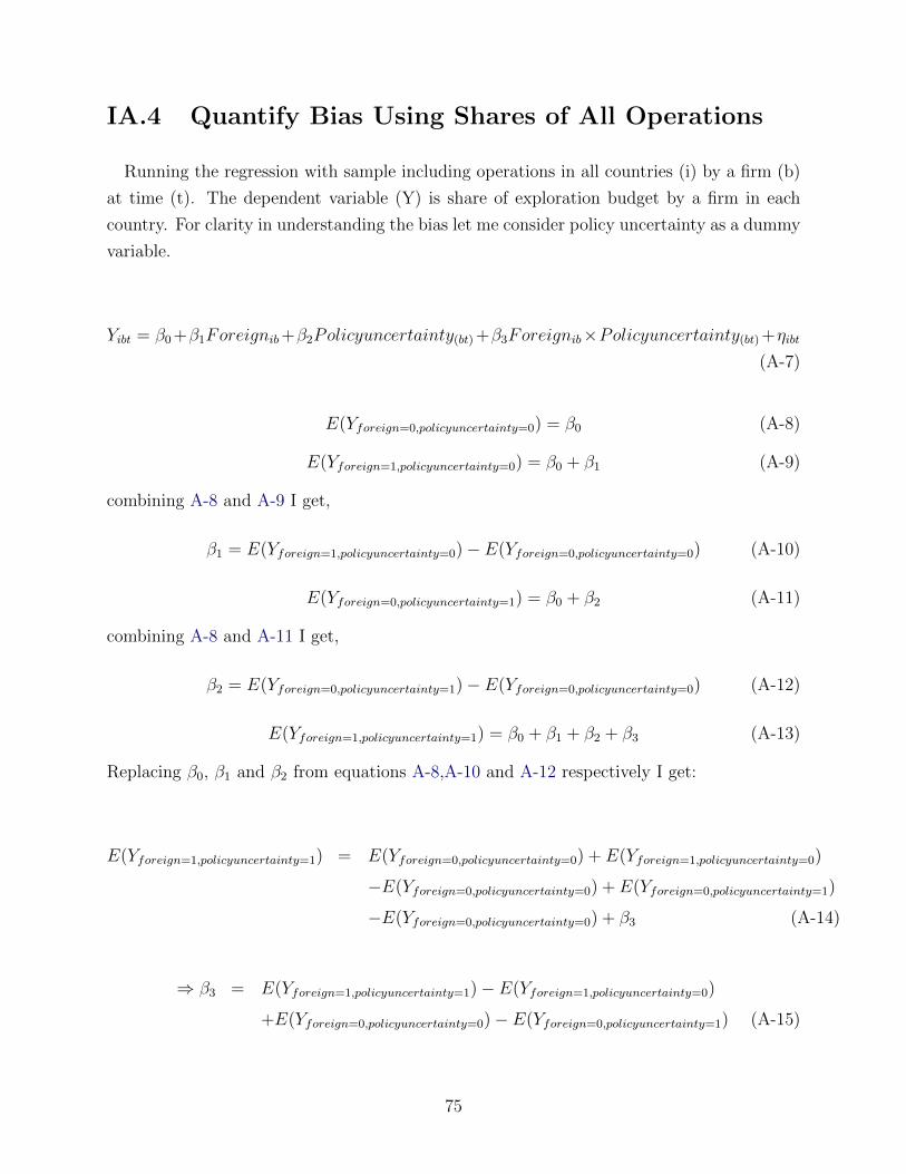
IA.4 Quantify Bias Using Shares of All Operations

Running the regression with sample including operations in all countries (i) by a firm (b)

at time (t). The dependent variable (Y) is share of exploration budget by a firm in each

country. For clarity in understanding the bias let me consider policy uncertainty as a dummy

variable.

Yibt = β0+β1Foreignib+β2Policyuncertainty(bt)+β3Foreignib×Policyuncertainty(bt)+ηibt(A-7)

E(Yforeign=0,policyuncertainty=0) = β0 (A-8)

E(Yforeign=1,policyuncertainty=0) = β0 + β1 (A-9)

combining A-8 and A-9 I get,

β1 = E(Yforeign=1,policyuncertainty=0)− E(Yforeign=0,policyuncertainty=0) (A-10)

E(Yforeign=0,policyuncertainty=1) = β0 + β2 (A-11)

combining A-8 and A-11 I get,

β2 = E(Yforeign=0,policyuncertainty=1)− E(Yforeign=0,policyuncertainty=0) (A-12)

E(Yforeign=1,policyuncertainty=1) = β0 + β1 + β2 + β3 (A-13)

Replacing β0, β1 and β2 from equations A-8,A-10 and A-12 respectively I get:

E(Yforeign=1,policyuncertainty=1) = E(Yforeign=0,policyuncertainty=0) + E(Yforeign=1,policyuncertainty=0)

−E(Yforeign=0,policyuncertainty=0) + E(Yforeign=0,policyuncertainty=1)

−E(Yforeign=0,policyuncertainty=0) + β3 (A-14)

⇒ β3 = E(Yforeign=1,policyuncertainty=1)− E(Yforeign=1,policyuncertainty=0)

+E(Yforeign=0,policyuncertainty=0)− E(Yforeign=0,policyuncertainty=1) (A-15)

75

Rearranging I get,

β3 = [E(Yforeign=1,policyuncertainty=1)− E(Yforeign=1,policyuncertainty=0)]

−[E(Yforeign=0,policyuncertainty=1)− E(Yforeign=0,policyuncertainty=0)] (A-16)

Let [E(Yforeign=1,policyuncertainty=1)−E(Yforeign=1,policyuncertainty=0)] = δ, i.e Let there be a total

of ‘n+1’ countries, of which 1 group is non-foreign and n groups are foreign. So increase in

δ units of ‘n’ foreign groups is same as decline of δ units of all the other ‘n’ group combined.

So on an average the increase for each foreign group is δn. Consequently,

[E(Yforeign=1,policyuncertainty=1)− E(Yforeign=1,policyuncertainty=0)] =δ

n

Thus the equation (A-16) can be expressed as

β3 =δ

n− (−δ) = δ +

δ

n=n+ 1

nδ (A-17)

limn→∞

β3 = δ

76

IA.5 Conceptual Framework and Motivation

In the discussion that follows, I will lay out the comparative statistics from a simple model

that illustrates how multi-country firms allocate resources in response to shocks in policy

related uncertainty. As I have discussed before policy uncertainty can manifest itself either

through a rise in risk or through reduction in cash flow. Through this model I will highlight

that shock to risk and shock to cash flow in one region could have different effect o investment

decisions in other regions.

Consider a firm operating in n regions with each firm using ki amount of capital to trans-

form into production using the production function fi(ki). The production function satisfies

the standard regularity conditions, i.e. f ′i(ki) > 0, f ′′i (ki) < 0 and fi(0) = 0 ∀ i. The inada

conditions are satisfied. The price of input and output at each unit/ region of production

is exogenously given to firms as ri and pi respectively. The revenue that firms generate in

the next period is discounted using a discount factor of θi. θi captures the risk in a region.

Higher the uncertainty, higher is the discount rate ρi and consequently lower is θi. Firms

utilizes their cash (Ci)to pay for their inputs in each region. The firm makes a centralized

decision to allocate capital in its different units by reallocating budget from one production

unit to the other (Williamson (1975), Gertner, Scharfstein, and Stein (1994), Giroud and

Mueller (2017) among others). It is also important to note that given the decision making

is at the headquarter of firms, budget constraint at the overall firm level and not at the

individual unit level binds. A firm’s optimization problem thus takes the following form:

L =∑i

θiPifi(ki) + λ(∑

i

Ci −∑i

riki)

(A-18)

λ is the lagrange multiplier and is interpreted as the shadow cost of the constraints. The

Kuhn-Tucker conditions are:

θiPif′i(ki) = ri(λ) ∀i (A-19)∑

i

Ci −∑i

riki = 0 (A-20)

λ(∑

i

Ci −∑i

riki)

= 0 (A-21)

Policy uncertainty in a region can either increases the risk of operation in that region or re-

duce the total available cash to pay the factors of production. Consequently, for the purpose

of this paper I are interested in studying the effect of change in θi on kj and change in Ci on kj.

77

IA.5.1 Effect of change in θi on kj

Differentiating (A-19) w.r.t θi I get

Pif′i(ki) + θiPif

′′i (ki)

δkiδθi

= riδλiδθi

(A-22)

Differentiating (A-19) w.r.t θj I get

θiPif′′i (ki)

δkiδθj

= riδλiδθj

(A-23)

Differentiating (A-20) w.r.t θj I get

∑i 6=j

riδkiδθj

+ rjδkjδθj

= 0 (A-24)

Using δkiδθi

and δkiδθj

from (A-22) and (A-23) in (A-24) I get:

δλ

δθj=

rjf′j(kj)

θjf ′′j (kj)∑i

r2iθiPif ′′i (ki)

> 0 ∀i

δkjδθj

= −rjf′j(kj)

θjf ′′j (kj)

∑i 6=j

riθif ′′i (ki)∑

ir2i

θiPif ′′i (ki)

> 0

δkiδθj

=rjf′j(kj)

θjf ′′j (kj)

riθif ′′i (ki)∑i

r2iθiPif ′′i (ki)

< 0

Given θj = 11+ρj

,δθjδρj

= − 1(1+ρj)2

. This implies:

δkjδρj

< 0 &δkiδρj

> 0

Thus I find that if policy uncertainty leads to rise in risk of operation in a region, firms tend

to invest less in that region and invests relatively more in other region. The idea being that as

policy uncertainty increases, firms find it risky to invest, consequently it frees up resource to

invest in other regions.31 It is crucial to note that: 1) all the units of the firms produces final

31It is important to mention that the underlying assumption of binding budget constraint highlights thatthe firms were not operating at optimum in all its region else there would be no impact of uncertainty oncapital investments in other region.If the budget constraint does not bind then λ = 0. This implies from

78

output and not intermediary products, and 2) there is no input-output linkages between the

output of different plants of the firm. If either of the above would be true then I might not

get the results obtained above. The intuition is that if there is an uncertainty shock in region

i, investment in region i decreases. If this output is an input in the production function of

the region j then investment and consequently output may also reduce. Mining sector fulfills

both these criterion as each mines produces the final output of a mining company and the

resource extracted from one mine is not used as an input for the other mine. Thus mining

sector provides me a good laboratory for our empirical investigation.

IA.5.2 Effect of change in Ci on kj

Policy uncertainty can also manifest itself as real economic shock to the wealth / cash flow

of the firm in a region i could have a negative spillover and lead to reduction in investment

in all other units j 6= i (Giroud and Mueller (2017)).

Differentiating A-19 and A-20 with respect to Ci

δλ

δCi=

1∑i

r2iθiPif ′′i (ki)

< 0

δKj

δCi=

rjθiPjf ′′j (kj)

δλ

δCi

⇒ δKj

δCi=

riθjPjf ′′j (kj)

1∑i

r2iθiPif ′′i (ki)

> 0 ∀i

Thus I see that as cash flow in a region decreases, firms reduces their investment from all

regions. Consequently I see a difference in the effect of uncertainty shock or a negative cash

flow shock in a region i on the investment in region j. While the former implies positive

impact on investment in region j, the latter indicates negative spillover.

Thus, I see that whileδKj

δCi< 0,

δkjδρi

> 0. Hence, the impact of policy uncertainty in one

region and its impact on the other region through the allocation decision making of the firm

is not clear. This motivates the empirical investigation of the paper.

equation (A-23) θiPif′′i (ki)

δkiδθj

= 0. i.e δkiδθj

= 0

79