Policy Improvement: Between Black-Box Optimizationand Episodic Reinforcement Learning

Freek Stulp1,2, Olivier Sigaud3

1 Robotics and Computer Vision, ENSTA-ParisTech, Paris2 FLOWERS Research Team, INRIA Bordeaux Sud-Ouest, Talence, France

3 Institut des Systèmes Intelligents et de Robotique, Univ. Pierre Marie Curie CNRS UMR 7222, Paris

Abstract : Policy improvement methods seek to optimize the parameters of a policy with respectto a utility function. There are two main approaches to performing this optimization: reinforcementlearning (RL) and black-box optimization (BBO). In recent years, benchmark comparisons betweenRL and BBO have been made, and there have been several attempts to specify which approach worksbest for which types of problem classes. In this article, we make several contributions to this line ofresearch by: 1) Classifying several RL algorithms in terms of their algorithmic properties. 2) Showinghow the derivation of ever more powerful RL algorithms displays a trend towards BBO. 3) Continuingthis trend by applying two modifications to the state-of-the-art PI2 algorithm, which yields an algorithmwe denote PIBB. We show that PIBB is a BBO algorithm. 4) Demonstrating that PIBB achieves similaror better performance than PI2 on several evaluation tasks. 5) Analyzing why BBO outperforms RLon these tasks. Rather than making the case for BBO or RL – in general we expect their relativeperformance to depend on the task considered – we rather provide two algorithms in which such casescan be made, as the algorithms are identical in all respects except in being RL or BBO approaches topolicy improvement.

1 IntroductionOver the last two decades, the convergence speed and robustness of policy improvement methods has in-creased dramatically, such that they are now able to learn a variety of challenging robotic tasks (Theodorouet al., 2010; Rückstiess et al., 2010b; Tamosiumaite et al., 2011; Kober & Peters, 2011; Buchli et al., 2011;Stulp et al., 2012). Several underlying trends have accompanied this performance increase. The first isrelated to exploration, where there has been a transition from action perturbing methods, which perturbthe output of the policy at each time step, to parameter perturbing methods, which perturb the parametersof the policy itself (Rückstiess et al., 2010b). The second trend pertains to the parameter update, whichhas moved from gradient-based methods towards updates based on reward-weighted averaging (Stulp &Sigaud, 2012a).

A striking feature of these trends, described in detail in Section 2, is that they have moved reinforcementlearning (RL) approaches to policy improvement closer and closer to black-box optimization (BBO). Infact, two state-of-the-art algorithms that have been applied to policy improvement — PI2 (Theodorou et al.,2010) and CMA-ES (Hansen & Ostermeier, 2001) — are so similar that a line-by-line comparison of thealgorithms is feasible (Stulp & Sigaud, 2012a). The main difference is that whereas PI2 is an RL algorithm— it uses information about rewards received at each time step during exploratory policy executions —CMA-ES is a BBO algorithm — it uses only the total reward received during execution, which enables itto treat the utility function as a black box that returns one scalar value.

In this article, we make the relation between RL and BBO even more explicit by taking these trends one(ultimate) step further. We do so by introducing PIBB (in Section 3), which simplifies the exploration andparameter update methods of PI2. These modifications are consistent with PI2’s derivation from stochasticoptimal control. An important insight is that PIBB is actually a BBO algorithm, as discussed in Section 3.3.One of the main contributions of this article is thus to draw an explicit bridge from RL to BBO approachesto policy improvement.

We thus have a pair of algorithms — PI2 and PIBB— that use the same method for exploration (parameterperturbation) and parameter updating (reward-weighted averaging), and differ only in being RL (PI2) or

JFPDA 2013

BBO (PIBB) approaches to policy improvement. This opens the way to a more objective comparison ofRL/BBO algorithms than, for instance, comparing eNAC and CMA-ES (Heidrich-Meisner & Igel, 2008a;Rückstiess et al., 2010b), as eNAC is an action-perturbing, gradient-based RL algorithm, and CMA-ESis a parameter-perturbing, reward-weighted averaging BBO algorithm. If one is found to outperform theother on a particular task, does it do so due to the different parameter update methods? Or is it due tothe difference in the policy perturbation? Or because one is an RL method and the other BBO? Using thePI2/PIBB pair allows us to specifically investigate the latter question, whilst keeping the other algorithmicfeatures the same.

The PI2/PIBB pair may thus be the key to providing “[s]trong empirical evidence for the power of evo-lutionary RL and convincing arguments why certain evolutionary algorithms are particularly well suitedfor certain RL problem classes” (Heidrich-Meisner & Igel, 2008a), and could help verify or falsify thefive conjectures proposed by Togelius et al. (2009, Section 4.1), about which types of problems are par-ticularly suited for RL and BBO approaches to policy improvement. As a first step in this direction, wecompare the performance of PI2 and PIBB in terms of convergence speed and final cost on the evaluationtasks from (Theodorou et al., 2010) in Section 3. Although PIBB has equal or better performance than PI2

on these tasks, our aim in this article is not to make a case for either RL or BBO approaches to policyimprovement — in general we expect the most appropriate method to vary from task to task, as discussedin Section 5 — but rather to provide a pair of algorithms that makes such targeted comparisons possible inthe first place.

In summary, the main contributions of this article are: • Providing an overview and classification ofpolicy improvement algorithms. • Deriving PIBB by simplifying the perturbation and update methods ofPI2. • Empirically comparing PI2 and PIBB on the five tasks proposed by Theodorou et al. (2010), andshowing that PIBB has equal or superior performance. • Demonstrating that PIBB is a BBO algorithm. Inparticular, it is a special case of CMA-ES. • Providing an algorithmic pair (PI2 and PIBB) that are identicalexcept in being RL and BBO approaches to policy improvement, which opens the way to an objectivecomparison of RL and BBO.

The rest of this article is structured as follows. In the next section, we describe several policy improvementalgorithms, explain their key differences, and classify them according to these differences. In Section 3, weshow how PIBB is derived by applying two simplifications to PI2, and we compare the algorithms empiricallyon five tasks. The PIBB algorithm is analyzed more closely in Section 3.3; in particular, we show that PIBB

is a BBO algorithm, and discuss several reasons why it outperforms PI2 on the tasks used. In Section 6 wesummarize the main contributions of the article.

2 Background

In RL, the policy π maps states to actions. The optimal policy π∗ chooses the action that optimizes acumulative reward over time. When the state and actions sets of the system are continuous, a policy cannotbe represented by enumerating all actions, so parametric policy representations πθ are required, where θis a vector of parameters. Thus, finding the optimal policy π∗ corresponds to finding the optimal policyparameters θ∗, i.e. those that maximize cumulative reward. As finding the θ corresponding to the globaloptimum is generally too expensive, policy improvement methods are local methods that rather search fora local optimum of the expected reward.

In episodic RL, on which this article focusses, the learner executes a task until a terminal state is reached.Executing a policy from an initial state until the terminal state, called a “roll-out”, leads to a trajectory τ ,which contains information about the states visited, actions executed, and rewards received. Many policyimprovement methods use an iterative process of exploration, where the policy is executed K times leadingto trajectories τ k=1...K , and parameter updating, where the policy parameters θ are updated based on thisbatch of trajectories. This process is explained in more detail in the generic policy improvement loopin Figure 1.

In this section, we give an overview of algorithms that implement this loop. We distinguish between threemain classes of algorithms, based on whether their derivation is based mainly — they are not mutually ex-clusive — on principles based on lower bounds on the expected return (Section 2.1), path integral stochasticoptimal control (Section 2.2) or BBO (Section 2.3).

Policy Improvement: Between BBO and Episodic RL

execute policy πθ

parameter update

θinit

θnew

θ roll-out of policy πθ

generate perturbation

roll-out of policy πθ

generate perturbation

roll-out of policy πθ

generate perturbation

τ k=1...K

Figure 1: Generic policy improvement loop. In each iteration, the policy is executed K times. One execution of a policy is called a ‘Monte Carloroll-out’, or simply ‘roll-out’. Because the policy is perturbed (different perturbation methods are described in Section 2.1.3), each execution leads toslightly different trajectories in state/action space, and potentially different rewards. The exploration phase thus leads to a set of different trajectoriesτk=1...K . Based on these trajectories, policy improvement methods then update the parameter vector θ → θnew such that the policy is expected toincur lower costs/higher rewards. The process then continues with the new θnew as the basis for exploration.

2.1 Policy Improvement through Lower Bounds on the Expected Return

We now briefly describe three algorithms that build on one another to achieve ever more powerful pol-icy improvement methods, being REINFORCE (Williams, 1992), eNAC (Peters & Schaal, 2008a), andPOWER (Kober & Peters, 2011). These algorithms may be derived from a common framework based onthe lower bound on the expected return, as demonstrated by Kober & Peters (2011). In this section, wefocus on properties of the resulting algorithms, rather than on their derivations. Since these algorithms havealready been covered in extensive surveys (Peters & Schaal, 2008a, 2007; Kober & Peters, 2011), we donot present them in full detail here, as this does not serve the particular aim of this section.

An underlying assumption of the algorithms presented in Section 2.1 and 2.2 is that the policies arerepresented as ut = g(x, t)ᵀθ; g is a set of basis functions, for instance Gaussian kernels, θ are the policyparameters, x is the state, and t is time since the roll-out started.

2.1.1 REINFORCE

The REINFORCE algorithm (Williams, 1992) (“reward increment = nonnegative factor× offset reinforce-ment× characteristic eligibility”) uses a stochastic policy to foster exploration (1), where πθ(x) returns thenominal motor command1, and εt is a perturbation of this command at time t. In REINFORCE, this policyis executed K times with the same θ, and the states/actions/rewards that result from a roll-out are stored ina trajectory.

Given K such trajectories, the parameters θ are then updated by first estimating the gradient ∇θJ(θ) (2)of the expected return J(θ) = E

[∑Ni=1 rti |πθ

]. Here, the trajectories are assumed to be of equal length,

i.e. having N discrete time steps ti=1...N . The notation in (2) estimates the gradient ∇θdJ(θ) for each pa-rameter entry d in the vector θ separately. Riedmiller et al. (2007) provides a concise yet clear explanationhow to derive (2). The baseline (3) is chosen so that it minimizes the variation in the gradient estimate (Pe-ters & Schaal, 2008b). Finally, the parameters are updated through steepest gradient ascent (4), where theopen parameter α is a learning rate.

Policy perturbation during a roll-outut = πθ(x) + εt (1)

Parameter update, given K roll-outs

∇θdJ(θ) =1

K

K∑

k=1

N∑

i=1

i∑

j=1

∇θdlog π(utj ,k|xtj ,k)(rti,k − b

dti) (2)

bdti =

∑Kk=1

∑ij=1

(∇θd

log π(utj ,k|xtj ,k))2rti,k

∑Kk=1

∑ij=1

(∇θd

log π(utj ,k|xtj ,k))2

(3)

θnew = θ + α∇θJ(θ) (4)

1With this notation, the policy πθ(x) is actually deterministic. A truly stochastic policy is denoted asut ∼ πθ(u|x) = µ(x) + εt (Riedmiller et al., 2007), where µ(x) is a deterministic policy that returns the nominal com-mand. We use our notation for consistency with parameter perturbation, introduced in Section 2.1.3. For now, it is best to consider thesum πθ(x) + εt to be the stochastic policy, rather than just πθ(x).

JFPDA 2013

2.1.2 eNAC

One issue with REINFORCE is that it requires many roll-outs for one parameter update, and the resultingtrajectories cannot be reused for later updates. This is because we need to perform a roll-out each timewe want to compute

∑Ni=1[. . . ]rti in (2). Such methods are known as ‘direct policy search’ methods.

Actor-critic methods, such as “Episodic Natural Actor Critic” (eNAC), address this issues by using a valuefunction Vπθ as a more compact representation of long-term reward than sample episodes R(τ ), allowingthem to make more efficient use of samples.

In continuous state-action spaces, Vπθ cannot be represented exactly, but must be estimated from data.Actor-critic methods therefore update the parameters in two steps: 1) approximate the value function fromthe point-wise estimates of the cumulative rewards observed in the trajectories acquired from roll-outs ofthe policy; 2) update the parameters using the value function. In contrast, direct policy search updates theparameters directly using point-wise estimates2. The main advantage of having a value function is that itgeneralizes; whereas K roll-outs provide only K point-wise estimates of the cumulative reward, a valuefunction approximated from these K point-wise estimates is also able to provide estimates not observed inthe roll-outs.

Another issue is that in REINFORCE the ‘naive’, or ‘vanilla’3, gradient ∇θJ(θ) is sensitive to differ-ent scales in parameters. To find the true direction of steepest descent towards the optimum, independentof the parameter scaling, eNAC uses the Fischer information matrix F to determine the ‘natural gradi-ent’: θnew = θ + αF−1(θ)∇θJ(θ). In practice, the Fischer information matrix need not be computedexplicitly (Peters & Schaal, 2008a).

Thus, going from REINFORCE to eNAC represents a transition from direct policy search to actor-critic,and from vanilla to natural gradients.

2.1.3 POWER

REINFORCE and eNAC are both ‘action perturbing’ methods which perturb the nominal command ateach time step ut = unominal

t +εt, cf. (1). Action-perturbing algorithms have several disadvantages: 1) Sam-ples are drawn independently from one another at each time step, which leads to a very noisy trajectory inaction space (Rückstiess et al., 2010b). 2) Consecutive perturbations may cancel each other and are thuswashed out (Kober & Peters, 2011). The system also often acts as a low-pass filter, which further reducesthe effects of perturbations that change with a high frequency. 3) On robots, high-frequency changes inactions, for instance when actions represent motor torques, may lead to dangerous behavior, or damage tothe robot (Rückstiess et al., 2010b). 4) It causes a large variance in parameter updates, an effect whichgrows with the number of time steps (Kober & Peters, 2011).

The “Policy Learning by Weighting Exploration with the Returns” (POWER) algorithm therefore im-plements a different policy perturbation scheme first proposed by Rückstiess et al. (2010a), where theparameters θ of the policy, rather than its output, are perturbed, i.e. π[θ + εt](x) rather than πθ(x) + εt.

REINFORCE and eNAC estimate gradients, which is not robust when noisy, discontinuous utility func-tions are involved. Furthermore, they require the manual tuning of the learning rate α, which is notstraightforward, but critical to the performance of the algorithms (Theodorou et al., 2010; Kober & Peters,2011). The POWER algorithm proposed by Kober & Peters (2011) addresses these issues by using reward-weighted averaging, which rather takes a weighted average of a set of K exploration vectors εk=1...K asfollows:

Policy perturbation during a roll-outut = π[θ + εt](x), with εt ∼ N (0,Σ) (5)

Parameter update, given K roll-outs

Skti =

∑Nj=ir

kj (6)

θnew = θ +

(E

[N∑i=1

WSkti

])−1(E

[N∑i=1

WεtiSkti

])(7)

2The point-wise estimates are sometimes considered to be a special type of critic; in this article we use the term ‘critic’ only whenit is a function approximator.

3‘Vanilla’ refers to the canonical version of an entity. The origin of this expression lies in ice cream flavors; i.e. ‘plain vanilla’ vs.‘non-plain’ flavors, such as strawberry, chocolate, etc.

Policy Improvement: Between BBO and Episodic RL

≈ θ +

(K∑

k=1

N∑i=1

WtiSkti

)−1( K∑k=1

N∑i=1

WtiεktiS

kti

)(8)

with Wti = gtigᵀti(gᵀ

tiΣgti)

−1

where K refers to the number of roll-outs, and gti is a vector of the basis function activations at timeti. The update (8) may be interpreted as taking the average of the perturbation vectors εk, but weightingthem with Sk/

∑Kl=1 Sl, which is a normalized version of the reward-to-go Sk. Hence the name reward-

weighted averaging. An important property of reward-weighted averaging is that it follows the naturalgradient (Arnold et al., 2011), without having to actually compute the gradient or the Fischer informationmatrix. This leads to more robust updates.

The final main difference between REINFORCE/eNAC and POWER is that the former require roll-out trajectories to contain information about the state and actions, as they must compute ∇θlogπθ(ut|xt) toperform an update. In contrast, POWER only uses information about the rewards rt from the trajectory,as these are necessary to compute the expected return (6). The basis function g are parameters of thealgorithm, and must not be stored in the trajectory.

In summary, going from eNAC to POWER represents a transition from action perturbation to policyparameter perturbation, from estimating the gradient to reward-weighted averaging, and from actor-criticback to direct policy search (as in REINFORCE).

2.2 Policy Improvement with Path Integrals (PI2)The PI2 algorithm has its roots in path integral solutions of stochastic optimal control problems4. In particu-lar, PI2 is the application of Generalized Path Integral Control (GPIC) to parameterized policies (Theodorouet al., 2010). For the complete PI2 derivation we refer to Theodorou et al. (2010).

Policy perturbation during a roll-out (parameter perturbation)ut = π[θ + εt](xt), with εt ∼ N (0,Σ) (9)

Parameter update for each time step (reward-weighted averaging)

Skti = φk

tN +

N−1∑j=i

qktj +1

2

N−1∑j=i+1

(θ + Mtjεktj )

ᵀR(θ + Mtjεktj ) (10)

P kti =

e− 1λSkti∑K

k=1[e− 1λSkti ]

(11)

δθti =K∑

k=1

[Mti ε

kti P

kti

]with Mtj = R−1gtj gT

tj (gTtjR

−1gtj )−1 (12)

Weighted average over time steps

[δθ]b =

∑N−1i=0 (N − i) [wti ]b [δθti ]b∑N−1

i=0 (N − i) [wti ]b(13)

Actual parameter updateθnew = θ + δθ (14)

The cost-to-go S(τ i,k) is computed for each of the K roll-outs and each time step i = 1 . . . N . Theterminal cost φtN , immediate costs qti and command cost matrix R are task-dependent and provided bythe user. The command cost matrix regularizes the parameter vector θ by penalizing θᵀRθ. Mtj ,k is aprojection matrix onto the range space of gtj under the metric R−1, cf. (Theodorou et al., 2010). Theweight of a roll-out P (τ i,k) is computed as the normalized exponentiation of the cost-to-go. This assignshigh weights to low-cost roll-outs and vice versa. In PI2, the weight Pk is interpreted as a probability, whichfollows from applying the Feynman-Kac theorem to the stochastic optimal control problem, cf. (Theodorouet al., 2010). The key algorithmic step is in (12), where the parameter update δθ is computed for eachtime step i through probability weighted averaging over the exploration ε of all K trials. Trajectories withhigher probabilities, and thus lower costs, therefore contribute more to this parameter update, moving theparameters into regions of lower costs.

4Note that in the previous section, algorithms aimed at maximizing rewards. In optimal control, the convention is rather to definecosts, which should be minimized.

JFPDA 2013

A different parameter update δθti is computed for each time step. To acquire one parameter vectorθ, the time-dependent updates must be averaged over time, one might simply use the mean parametervector over all time steps: δθ = 1

N

∑Ni=1 δθti . Although temporal averaging is necessary, the particular

weighting scheme used in temporal averaging does not follow from the derivation. Rather than a simplemean, Theodorou et al. (2010) suggest the weighting scheme in Eq. (13). It emphasizes updates earlier inthe trajectory, and also makes use of the activation of the jth basis function at time step i, i.e. wj,ti .

As demonstrated in (Theodorou et al., 2010), PI2 is able to outperform the previous RL algorithms forparameterized policy learning described in Section 2.1 by at least one order of magnitude in learning speed(number of roll-outs to converge) and also lower final cost performance. As an additional benefit, PI2 hasno open algorithmic parameters, except for the magnitude of the exploration noise Σ, and the number oftrials per update K.

Although having been derived from very different principles, PI2 and POWER use identical policy per-turbation methods, and have very similar update rules. The main difference between them is that POWERrequires the cost function to behave as improper probability, i.e. be strictly positive and integrate to a con-stant number. This constraint can make the design of suitable cost functions more complicated (Theodorouet al., 2010). For cost functions with the same optimum in POWER’s pseudo-probability formulation andPI2 cost function, “both algorithms perform essentially identical” (Theodorou et al., 2010). Another differ-ence is that matrix inversion in POWER’s parameter update (8) is not necessary in PI2.

2.3 Policy Improvement through Black-box OptimizationPolicy improvement may also be achieved with BBO. In general, the aim of BBO is to find the solutionx∗ ∈ X that optimizes the objective function J : X 7→ R (Arnold et al., 2011). As in stochastic optimalcontrol and PI2, J is usually chosen to be a cost function, such that optimization corresponds to minimiza-tion. Let us highlight three aspects that define BBO: 1) Input: no assumptions are made about the searchspace X; 2) Objective function: the function J is treated as a ‘black box’, i.e. no assumptions are madeabout, for instance, its differentiability or continuity; 3) Output: the objective function returns only onescalar value. A desirable property of BBO algorithms that are applicable to problems with these conditionsis that they are able to find x∗ using as few samples from the objective function J(x) as possible. ManyBBO algorithms, such as CEM (Rubinstein & Kroese, 2004), CMA-ES (Hansen & Ostermeier, 2001) andNES (Wierstra et al., 2008), use an iterative strategy, where the current x is perturbed x + εk=1...K , and anew solution xnew is computed given the evaluations Jk=1...K = J(x + εk=1...K).

BBO is applicable to policy improvement (Rückstiess et al., 2010b) as follows: 1) Input: the input xis interpreted as being the policy parameter vector θ. Whereas RL algorithms are tailored to leveragingthe problem structure to update the policy parameters θ, BBO algorithms used for policy improvement arecompletely agnostic about what the parameters θ represent; θ might represent the policy parameters fora motion primitive to grasp an object, or simply the 2-D search space to find the minimum of a quadraticfunction. 2) Objective function: the function f executes the policy π with parameters θ, and records therewards rti=1:N

. 3) Output: J must sum over these rewards after a policy execution: R =∑Ni=1 rti to

achieve an output of only one scalar value. Examples of applying BBO to policy improvement include (Ng& Jordan, 2000; Busoniu et al., 2011; Heidrich-Meisner & Igel, 2008a; Rückstiess et al., 2010b; Marin &Sigaud, 2012; Fix & Geist, 2012).

For the point of view of policy improvement, an important property of BBO algorithms is that the searchis performed in the space of policy parameters; this is the input of the black-box cost function J . Therefore,all BBO approaches to policy improvement must be policy parameter perturbing methods. Furthermore,since the policy is executed within the function J , the parameter perturbation θ+ε can be passed only onceas an argument to J before the policy is executed. The perturbations ε therefore cannot vary over time,as is the case in REINFORCE/eNAC/POWER. As Heidrich-Meisner & Igel (2008a) note: “in evolution-ary strategies [BBO] there is only one initial stochastic variation per episode, while the stochastic policyintroduces perturbations in every step of the episode.”.

The RL algorithms discussed in Section 2.1 (REINFORCE/eNAC/POWER) and 2.2 (PI2), use informa-tion about the rewards received at each time step. Furthermore, REINFORCE/eNAC also use informationabout the states visited, and actions executed in these states. BBO by definition cannot make use of thisinformation, because the black-box cost function returns only a scalar cost, as visualized in Figure 2. Forpolicy improvement, this scalar cost is taken to be the return of an episode R =

∑Ni=1 rti .

In fact, if a policy improvement algorithm 1) uses policy perturbation, where the perturbation is constant

Policy Improvement: Between BBO and Episodic RL

rt1 rt2 . . . rtNxt1 xt2 . . . xtN

ut1 ut2 . . . utN

rt1 rt2 . . . rtN

only rewardsstates/actions/rewards

∑N J

aggregrate scalar reward

Figure 2: Illustration of the different types of information that may be stored in the trajectories that arise from policy roll-outs. Algorithms that use onlythe aggregate scalar reward are considered to be BBO approaches to policy improvement.

during policy execution, and 2) stores only the scalar total cost of a roll-out in the trajectory, then it is bydefinition a BBO approach to policy improvement, because the algorithm that works under these conditionsis by definition a BBO algorithm. If a particular algorithm is historically considered to be an RL approach,we are agnostic about this. But if the two conditions above (one scalar return, constant parameter pertur-bation) hold, it must at least be acknowledged that the algorithm may also be interpreted as being a BBOalgorithm. As Rückstiess et al. (2010b) point out: “the return of a whole RL episode can be interpretedas a single fitness evaluation. In this case, parameter-based exploration in RL is equivalent to black-boxoptimization.”.

The relative advantages and disadvantages of using the states and rewards encountered during a roll-outrather than treating policy improvement as BBO depend on the domain and problem structure, and are notyet well understood (Heidrich-Meisner & Igel, 2008a).

2.3.1 BBO Algorithms Applied to Policy Improvement

CMA-ES (Hansen & Ostermeier, 2001) is an example of an existing BBO method that was applied onlymuch later to the specific domain of policy improvement (Heidrich-Meisner & Igel, 2008a). In BBO,CMA-ES is considered to be a de facto standard (Rückstiess et al., 2010b).

Further BBO algorithms that have been applied to policy improvement include the Cross-Entropy Method(CEM) (Rubinstein & Kroese, 2004; Busoniu et al., 2011; Heidrich-Meisner & Igel, 2008b), which isvery similar to CMA-ES, but has simpler methods for determining the weights Pk and performing thecovariance matrix update. For a comparison of further BBO algorithms such as PGPE (Rückstiess et al.,2010b) and Natural Evolution Strategies (NES) (Wierstra et al., 2008) with CMA-ES and eNAC, pleasesee the overview article by Rückstiess et al. (2010b).

NEAT+Q is a hybrid algorithm that actually combines RL and BBO in a very original way (Whiteson &Stone, 2006). Within our classification, NEAT+Q is first and foremost an actor-critic approach, as func-tion approximation is used to explicitly represent the value function. What sets NEAT+Q apart is that therepresentation of the value function is evolved through BBO, with the “Neuro Evolution of AugmentingTopologies” (NEAT). This alleviates the user from having to design this representation; unsuitable repre-sentations may keep RL algorithms from being able to learn the problem, even for algorithms with provenconvergence properties (Whiteson & Stone, 2006).

2.4 Classification of Policy Improvement AlgorithmsBased on several of the properties of the algorithms discussed in this section, we provide a classificationof these algorithms in Figure 3. The figure also depicts the aim of the next section: simplifying the PI2

algorithm to acquire PIBB, which is a BBO algorithm.

3 From PI2 to PIBB

To convert PI2 to a BBO algorithm, we must first adapt the policy perturbation method. PI2 and BBO bothuse policy parameter perturbation, but in PI2 it varies over time (θ + εt), whereas it must remain constantover time in BBO (θ + ε). In Section 3.1, we therefore simplify the perturbation method in PI2 to beconstant over time, which yields the algorithm variation PI2 .

Second, we must adapt PI2 such that it is able to update the parameters based only on the scalar aggregatedcost J =

∑Ni=1 rti , rather than having access to the reward rt at each time step t. This is done in Section 3.2,

and yields the PIBB algorithm. An important aspect of these two simplifications for deriving PIBB from PI2

JFPDA 2013

Trajectory? states/actions/rewards(at each time step)

rewards only(at each time step) (aggregrated)

Perturbation? action(at each time step)

parameter(at each time step) (constant)

Actor-Critic? act.-critic direct policy search

Upd

ate?

vanillagradient

naturalgradient

reward-w.averaging PIBB

REINFORCE

eNAC

POWER

GPIC PI2

FD

PGPE

NES

CMA-ESCEM

Figure 3: Classification of policy improvement algorithms. The vertical dimension categorizes the update method used, and the horizontal dimensionthe method used to perturb the policy. The two streams represent both the derivation history of policy improvement algorithms.

is that they do not violate any of the assumptions required for the derivation of PI2 from stochastic optimalcontrol, which we motivate in more detail throughout this section.

3.1 Simplifying the Exploration MethodThis section is concerned with analyzing exploration in PI2. We refer to the ‘canonical’ version of PI2,which samples different exploration vectors εt for each time step, as PI2 . The small blue symbol servesas a mnemonic to indicate that exploration varies at a high frequency. As an alternative to time-varyingexploration, Theodorou et al. (2010) propose to generate exploration noise only for the basis function withthe highest activation. This approach is also used by Tamosiumaite et al. (2011). We refer to this secondmethod as PI2 with exploration per basis function, or PI2 , where the green graphs serves as a mnemonic ofthe shape of the exploration for one basis function. Alternatively, εti,k can be set to have a constant valueduring a roll-out (Stulp & Sigaud, 2012a). Thus, for each of the K roll-outs, we generate εk explorationvectors before executing the policy, and keep it constant during the execution, i.e. εti,k = εk. We call this‘PI2 with constant exploration’, and denote it as PI2 , where the horizontal line indicates a constant valueover time.

3.2 Simplifying the Parameter UpdateIn this section, we simplify the parameter update rule of PI2 which yields the simpler PIBB algorithm.

In PI2, a different parameter update δθti is computed for each time step i. This is caused by its derivationfrom GPIC, where motor commands ut are different at each time step; it is difficult to imagine a task thatrequires a constant motor command during a roll-out. But since the policy parameters θ are constant duringa roll-out, there is a need to condense the N parameters updates δθti=0:N into one update δθ. This step iscalled temporal averaging, and was proposed by Theodorou et al. (2010) as:

[δθ]d =

∑Ni=1(N − i+ 1) wd,ti [δθti ]d∑N

i=1 wd,ti(N − i+ 1). (15)

This temporal averaging scheme emphasizes updates earlier in the trajectory, and also makes use of thebasis function weights wd,ti . However, since this does not directly follow from the derivation “[u]sersmay develop other weighting schemes as more suitable to their needs.” (Theodorou et al., 2010). As analternative, we now choose a weight of 1 at the first time step, and 0 for all others. This means that allupdates δθti are ignored, except the first one δθt1 , which is based on the cost-to-go at the first time stepS(τ 1,k). By definition, the cost-to-go at t1 represents the cost of the entire trajectory. This implies thatwe must only compute the cost-to-go S(τ i,k) and probability P (τ i,k) for i = 1. This simplified PI2

variant, which does not use temporal averaging, and which we denote ‘PIBB’ is presented in more detail inSection 3.3.

Policy Improvement: Between BBO and Episodic RL

Note that this simplification depends strongly on using constant exploration noise during a roll-out. Ifthe noise varies at each time step or per basis function, the variation at the first time step εt1,k is not atall representative for the variations throughout the rest of the trajectory. It is therefore more accurate toconsider PIBB as a variant of PI2 , rather than of PI2 ≡PI2 .

3.3 The PIBB Algorithm

PIBB is a special case of PI2 in which: 1) Exploration noise is constant over time, i.e. as in PI2 . 2) Temporalaveraging uses only the first update, i.e. δθnew = δθnew

t1 . We also refer to this simply as ‘no temporalaveraging’. In this section, we perform a closer analysis of PIBB.

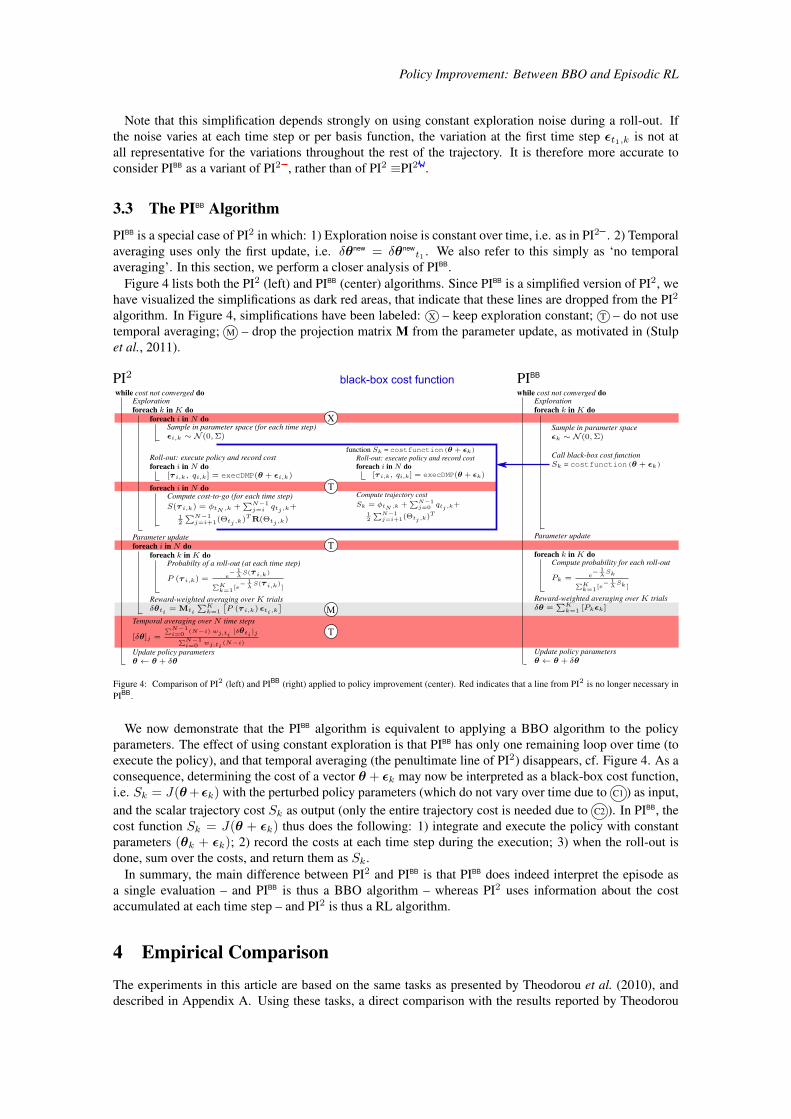
Figure 4 lists both the PI2 (left) and PIBB (center) algorithms. Since PIBB is a simplified version of PI2, wehave visualized the simplifications as dark red areas, that indicate that these lines are dropped from the PI2

algorithm. In Figure 4, simplifications have been labeled: X – keep exploration constant; T – do not usetemporal averaging; M – drop the projection matrix M from the parameter update, as motivated in (Stulpet al., 2011).

Figure 4: Comparison of PI2 (left) and PIBB (right) applied to policy improvement (center). Red indicates that a line from PI2 is no longer necessary inPIBB.

We now demonstrate that the PIBB algorithm is equivalent to applying a BBO algorithm to the policyparameters. The effect of using constant exploration is that PIBB has only one remaining loop over time (toexecute the policy), and that temporal averaging (the penultimate line of PI2) disappears, cf. Figure 4. As aconsequence, determining the cost of a vector θ + εk may now be interpreted as a black-box cost function,i.e. Sk = J(θ+εk) with the perturbed policy parameters (which do not vary over time due to C1 ) as input,and the scalar trajectory cost Sk as output (only the entire trajectory cost is needed due to C2 ). In PIBB, thecost function Sk = J(θ + εk) thus does the following: 1) integrate and execute the policy with constantparameters (θk + εk); 2) record the costs at each time step during the execution; 3) when the roll-out isdone, sum over the costs, and return them as Sk.

In summary, the main difference between PI2 and PIBB is that PIBB does indeed interpret the episode asa single evaluation – and PIBB is thus a BBO algorithm – whereas PI2 uses information about the costaccumulated at each time step – and PI2 is thus a RL algorithm.

4 Empirical ComparisonThe experiments in this article are based on the same tasks as presented by Theodorou et al. (2010), anddescribed in Appendix A. Using these tasks, a direct comparison with the results reported by Theodorou

JFPDA 2013

et al. (2010) is straightforward. Furthermore, it alleviates us of the need to demonstrate that PI2 outperformsREINFORCE, eNAC and POWER on these tasks, because this was already done by Theodorou et al.(2010).

For each learning session, we are interested in comparing the convergence speed and final cost, i.e. thevalue to which the learning curve converges. Convergence speed is measured as the parameter update afterwhich the cost drops below 5% of the initial cost before learning. The final cost is the mean cost over the last100 updates. For all tasks and algorithm settings, we execute 10 learning sessions (which together we callan ‘experiment’), and report the µ ± σ over these 10 learning sessions. For all experiments, the DynamicMovement Primitives (DMPs) (Ijspeert et al., 2002) and PI2 parameters are the same as in (Theodorouet al., 2010), and listed in Appendix A.

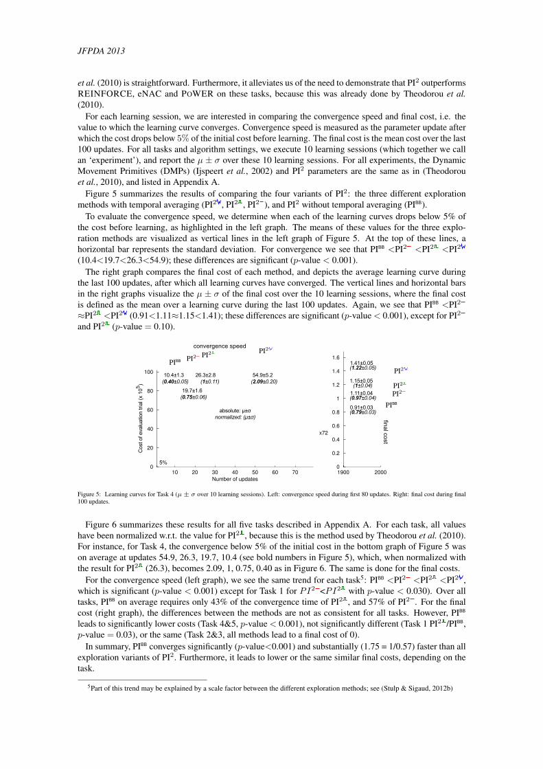
Figure 5 summarizes the results of comparing the four variants of PI2: the three different explorationmethods with temporal averaging (PI2 , PI2 , PI2 ), and PI2 without temporal averaging (PIBB).

To evaluate the convergence speed, we determine when each of the learning curves drops below 5% ofthe cost before learning, as highlighted in the left graph. The means of these values for the three explo-ration methods are visualized as vertical lines in the left graph of Figure 5. At the top of these lines, ahorizontal bar represents the standard deviation. For convergence we see that PIBB <PI2 <PI2 <PI2

(10.4<19.7<26.3<54.9); these differences are significant (p-value < 0.001).The right graph compares the final cost of each method, and depicts the average learning curve during

the last 100 updates, after which all learning curves have converged. The vertical lines and horizontal barsin the right graphs visualize the µ ± σ of the final cost over the 10 learning sessions, where the final costis defined as the mean over a learning curve during the last 100 updates. Again, we see that PIBB <PI2

≈PI2 <PI2 (0.91<1.11≈1.15<1.41); these differences are significant (p-value < 0.001), except for PI2

and PI2 (p-value = 0.10).

Figure 5: Learning curves for Task 4 (µ ± σ over 10 learning sessions). Left: convergence speed during first 80 updates. Right: final cost during final100 updates.

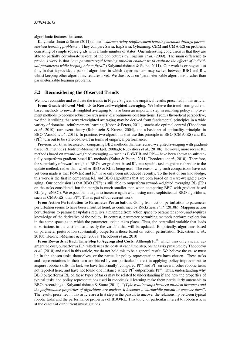
Figure 6 summarizes these results for all five tasks described in Appendix A. For each task, all valueshave been normalized w.r.t. the value for PI2 , because this is the method used by Theodorou et al. (2010).For instance, for Task 4, the convergence below 5% of the initial cost in the bottom graph of Figure 5 wason average at updates 54.9, 26.3, 19.7, 10.4 (see bold numbers in Figure 5), which, when normalized withthe result for PI2 (26.3), becomes 2.09, 1, 0.75, 0.40 as in Figure 6. The same is done for the final costs.

For the convergence speed (left graph), we see the same trend for each task5: PIBB <PI2 <PI2 <PI2 ,which is significant (p-value < 0.001) except for Task 1 for PI2 <PI2 with p-value < 0.030). Over alltasks, PIBB on average requires only 43% of the convergence time of PI2 , and 57% of PI2 . For the finalcost (right graph), the differences between the methods are not as consistent for all tasks. However, PIBB

leads to significantly lower costs (Task 4&5, p-value < 0.001), not significantly different (Task 1 PI2 /PIBB,p-value = 0.03), or the same (Task 2&3, all methods lead to a final cost of 0).

In summary, PIBB converges significantly (p-value<0.001) and substantially (1.75 = 1/0.57) faster than allexploration variants of PI2. Furthermore, it leads to lower or the same similar final costs, depending on thetask.

5Part of this trend may be explained by a scale factor between the different exploration methods; see (Stulp & Sigaud, 2012b)

Policy Improvement: Between BBO and Episodic RL

Figure 6: Results for all tasks, normalized w.r.t. PI2 . Left: convergence speed. Right: final cost.

5 DiscussionSo why, on these five tasks, is PI2 outperformed by the much simpler BBO algorithm PIBB? It is rathercounter-intuitive that an algorithm that uses less information is able to converge as fast or quicker than analgorithm that uses more information. This intuition is captured well in the following quote from Moriartyet al. (1999) “In this sense, EA [BBO] methods pay less attention to individual decisions than TD [RL]methods do. While at first glance, this approach appears to make less efficient use of information, it may infact provide a robust path toward learning good policies.”

In this discussion section, we first describe previous comparisons of RL and BBO algorithms, and thenexplain how our results extend the knowledge obtained in this previous work. In particular, we re-considerthe trends in Figure 3. We also discuss how the results we have obtained are influenced by the choice ofpolicy representation and tasks used by Theodorou et al. (2010) and ourselves, which are tailored to thedomain of learning skills on physical robots.

5.1 Previous Work on Empirically Comparing RL and BBO

The earliest empirical comparison of RL and BBO that we are aware of is the work of Moriarty et al.(1999). They compare “Evolutionary Algorithms for Reinforcement Learning” (EARL) with Q-learning ona simple MDP grid world, and conclude that these two methods “while complementary approaches, are byno means mutually exclusive.” and that BBO approaches are advantageous “in situations where the sensorsare inadequate to observe the true state of the world.” (Moriarty et al., 1999).

Heidrich-Meisner & Igel (2008b) compare the performance of CMA-ES and NAC on a single pole bal-ancing task. They conclude that “Our preliminary comparisons indicate that the CMA-ES is more robustw.r.t. to the choice of hyperparameters and initial policies. In terms of learning speed, the natural policygradient ascent performs on par for fine-tuning and may be preferable in this scenario.” This work was laterextended to a double pole balancing task (Heidrich-Meisner & Igel, 2008a), where similar conclusions weredrawn. A more extensive evaluation on single- and double pole balancing tasks is performed by (Gomezet al., 2008). They also conclude that “in real world control problems, neuroevolution [. . . ] can solve theseproblems much more reliably and efficiently than non-evolutionary reinforcement learning approaches”.

In an extensive comparison, Rückstiess et al. (2010b) compare PGPE, REINFORCE, NES, eNAC,NES and CMA-ES on pole-balancing, biped standing, object grasping, and ball catching. Their focus isparticularly on comparing action-perturbing and parameter-perturbing algorithms. Their main conclusion isthat parameter-perturbation outperforms action-perturbation: “We believe that parameter-based explorationshould play a more important role not only for [policy gradient] methods but for continuous RL in general,and continuous value-based RL in particular” (Rückstiess et al., 2010b).

An issue with such comparisons is that “each of these efforts typically only compares a few algorithms ona single problem, leading to contradictory results regarding the merits of different RL methods.” (Togeliuset al., 2009). It is this issue that we referred to in the introduction: if CMA-ES outperforms eNAC ona particular task, is it because of their different perturbation methods, their different parameter updatemethods, or because one is BBO and the other is RL? One of the main results of this article is to provide analgorithmic framework that allows us to specifically investigate the latter question, whilst keeping the other

JFPDA 2013

algorithmic features the same.Kalyanakrishnan & Stone (2011) aim at “characterizing reinforcement learning methods through param-

eterized learning problems”. They compare Sarsa, ExpSarsa, Q-learning, CEM and CMA-ES on problemsconsisting of simple square grids with a finite number of states. One interesting conclusion is that they areable to partially corroborate several of the conjectures by Togelius et al. (2009). The main difference toprevious work is that “our parameterized learning problem enables us to evaluate the effects of individ-ual parameters while keeping others fixed.” (Kalyanakrishnan & Stone, 2011). Our work is orthogonal tothis, in that it provides a pair of algorithms in which experimenters may switch between BBO and RL,whilst keeping other algorithmic features fixed. We thus focus on ‘parameterizable algorithms’, rather thanparameterizable learning problems.

5.2 Reconsidering the Observed TrendsWe now reconsider and evaluate the trends in Figure 3, given the empirical results presented in this article.

From Gradient-based Methods to Reward-weighted averaging. We believe the trend from gradient-based methods to reward-weighted averaging to have been an important step in enabling policy improve-ment methods to become robust towards noisy, discontinuous cost functions. From a theoretical perspective,we find it striking that reward-weighted averaging may be derived from fundamental principles in a widevariety of domains: reinforcement learning (Kober & Peters, 2011), stochastic optimal control (Theodorouet al., 2010), rare-event theory (Rubinstein & Kroese, 2004), and a basic set of optimality principles inBBO (Arnold et al., 2011). In practice, two algorithms that use this principle in BBO (CMA-ES) and RL(PI2) turn out to be state-of-the-art in terms of empirical performance.

Previous work has focussed on comparing BBO methods that use reward-weighted averaging with gradient-based RL methods (Heidrich-Meisner & Igel, 2008a,b; Rückstiess et al., 2010b). However, more recent RLmethods based on reward-weighted averaging — such as POWER and PI2— have been shown to substan-tially outperform gradient-based RL methods (Kober & Peters, 2011; Theodorou et al., 2010). Therefore,the superiority of reward-weighted BBO over gradient-based RL on a specific task might be rather due to theupdate method, rather than whether BBO or RL is being used. The reason why such comparisons have notyet been made is that POWER and PI2 have only been introduced recently. To the best of our knowledge,this work is the first in comparing RL and BBO algorithms that are both based on reward-weighted aver-aging. Our conclusion is that BBO (PIBB) is still able to outperform reward-weighted averaging RL (PI2)on the tasks considered, but the margin is much smaller than when comparing BBO with gradient-basedRL (e.g. eNAC). We expect this margin to increase again when using more sophisticated BBO algorithms,such as CMA-ES, than PIBB. This is part of our current work.

From Action Perturbation to Parameter Perturbation. Going from action perturbation to parameterperturbation seems to have been a fruitful trend, as confirmed by Rückstiess et al. (2010b). Mapping actionperturbations to parameter updates requires a mapping from action space to parameter space, and requiresknowledge of the derivative of the policy. In contrast, parameter perturbing methods perform explorationin the same space as in which the parameter update takes place. Thus, the controlled variable that leadsto variations in the cost is also directly the variable that will be updated. Empirically, algorithms basedon parameter perturbation substantially outperform those based on action perturbation (Rückstiess et al.,2010b; Heidrich-Meisner & Igel, 2008a; Theodorou et al., 2010).

From Rewards at Each Time Step to Aggregrated Costs. Although PIBB, which uses only a scalar ag-gregrated cost, outperforms PI2, which uses the costs at each time step, on the tasks presented by Theodorouet al. (2010) and used in this article, we do not hold this to be a general result. We believe the cause mustlie in the chosen tasks themselves, or the particular policy representation we have chosen. These tasksand representations in their turn are biased by our particular interest in applying policy improvement toacquire robotic skills. In fact, we have (informally) compared PIBB and PI2 on several other robotic tasksnot reported here, and have not found one instance where PI2 outperforms PIBB. Thus, understanding whyBBO outperforms RL on these types of tasks may be related to understanding if and how the properties oftypical tasks and policy representations used in robotic skill learning make them particularly amenable toBBO. According to Kalyanakrishnan & Stone (2011): “[T]he relationships between problem instances andthe performance properties of algorithms are unclear, it becomes a worthwhile pursuit to uncover them”.The results presented in this article are a first step in the pursuit to uncover the relationship between typicalrobotic tasks and the performance properties of BBO/RL. This topic, of particular interest to roboticists, isat the center of our current investigations.

Policy Improvement: Between BBO and Episodic RL

6 ConclusionWe have provided a classification of policy improvement algorithms. Furthermore, within this classification,we observed three trends in the chronology and derivation paths of algorithms: from gradient-based methodsto reward-weighted averaging, from action to parameter perturbation, and towards algorithms that use onlyreward information from policy roll-outs. We observe that these trends have brought RL methods closerand closer to BBO approaches to policy improvement.

In previous work, it was shown that PI2 is able to outperform PEGASUS, REINFORCE, eNAC andPOWER (Theodorou et al., 2010). Using exactly the same tasks, we observe rather surprisingly that themuch simpler BBO algorithm PIBB has equal or better performance than PI2 still. Previous work on compar-ing RL and BBO shows that BBO often wins by a wide margin; the caveat being that, in those experiments,the BBO methods use reward-weighted averaging whereas the RL methods use gradient estimation. Animportant conclusion of our results is that the margin, though still existent, is much smaller when both RLand BBO are based on the powerful concept of reward-weighted averaging.

But rather than making the case for BBO or RL, one of the main contributions of this article is to providean algorithmic framework in which such cases may be made. Because PIBB and PI2 use identical perturbationand parameter update methods, and differ only in being BBO and RL approaches respectively, this facilitatesa more objective comparison of BBO and RL than for instance comparing algorithms that differ in manyrespects. Therefore, we believe this algorithmic pair is an excellent basis for comparing BBO and RLapproaches to policy improvement, and further investigating the five conjectures in (Togelius et al., 2009).

Although BBO thus trumps RL on the tasks we consider, we do not believe this to be a general result, andfurther investigations are needed, especially into the bias that typical tasks and policy representations usedin robotics – the types used in this article – introduce into RL problems.

ReferencesARNOLD L., AUGER A., HANSEN N. & OLLIVIER Y. (2011). Information-Geometric Optimization Al-

gorithms: A Unifying Picture via Invariance Principles. Rapport interne, INRIA Saclay.BUCHLI J., STULP F., THEODOROU E. & SCHAAL S. (2011). Learning variable impedance control.

International Journal of Robotics Research, 30(7), 820–833.BUSONIU L., ERNST D., SCHUTTER B. D. & BABUSKA R. (2011). Cross-entropy optimization of control

policies with adaptive basis functions. IEEE Transactions on Systems, Man, and Cybernetics-Part B:Cybernetics, 41(1), 196–209.

FIX J. & GEIST M. (2012). Monte-carlo swarm policy search. In Symposium on Swarm Intelligence andDifferential Evolution, Lecture Notes in Artificial Intelligence (LNAI), p. 9 pages. Zakopane (Poland):Springer Verlag - Heidelberg Berlin.

GOMEZ F., SCHMIDHUBER J. & MIIKKULAINEN R. (2008). Accelerated neural evolution through coop-eratively coevolved synapses. Journal of Machine Learning Research, 9, 937–965.

HANSEN N. & OSTERMEIER A. (2001). Completely derandomized self-adaptation in evolution strategies.Evolutionary Computation, 9(2), 159–195.

HEIDRICH-MEISNER V. & IGEL C. (2008a). Evolution strategies for direct policy search. In Proceedingsof the 10th international conference on Parallel Problem Solving from Nature: PPSN X, p. 428–437,Berlin, Heidelberg: Springer-Verlag.

HEIDRICH-MEISNER V. & IGEL C. (2008b). Similarities and differences between policy gradient methodsand evolution strategies. In ESANN 2008, 16th European Symposium on Artificial Neural Networks,Bruges, Belgium, April 23-25, 2008, Proceedings, p. 149–154.

IJSPEERT A. J., NAKANISHI J. & SCHAAL S. (2002). Movement imitation with nonlinear dynamicalsystems in humanoid robots. In Proceedings of the IEEE International Conference on Robotics andAutomation (ICRA).

KALYANAKRISHNAN S. & STONE P. (2011). Characterizing reinforcement learning methods throughparameterized learning problems. Machine Learning, 84(1-2), 205–247.

KOBER J. & PETERS J. (2011). Policy search for motor primitives in robotics. Machine Learning, 84,171–203.

MARIN D. & SIGAUD O. (2012). Towards fast and adaptive optimal control policies for robots: A directpolicy search approach. In Proceedings Robotica, p. 21–26, Guimaraes, Portugal.

JFPDA 2013

MORIARTY D. E., SCHULTZ A. C. & GREFENSTETTE J. J. (1999). Evolutionary algorithms for rein-forcement learning. Journal of Artificial Intelligence (JAIR), 11, 241–276.

NG A. Y. & JORDAN M. I. (2000). Pegasus: A policy search method for large mdps and pomdps. InProceedings of the 16th Conference on Uncertainty in Artificial Intelligence, p. 406–415.

PETERS J. & SCHAAL S. (2007). Applying the episodic natural actor-critic architecture to motor primitivelearning. In Proceedings of the 15th European Symposium on Artificial Neural Networks (ESANN 2007),p. 1–6.

PETERS J. & SCHAAL S. (2008a). Natural actor-critic. Neurocomputing, 71(7-9), 1180–1190.PETERS J. & SCHAAL S. (2008b). Reinforcement learning of motor skills with policy gradients. Neural

networks : the official journal of the International Neural Network Society, 21(4), 682–97.POWELL W. B. (2007). Approximate Dynamic Programming: Solving the curses of dimensionality, volume

703. Wiley-Blackwell.RIEDMILLER M., PETERS J. & SCHAAL S. (2007). Evaluation of Policy Gradient Methods and Vari-

ants on the Cart-Pole Benchmark. In 2007 IEEE International Symposium on Approximate DynamicProgramming and Reinforcement Learning, p. 254–261: IEEE.

RUBINSTEIN R. & KROESE D. (2004). The Cross-Entropy Method: A Unified Approach to CombinatorialOptimization, Monte-Carlo Simulation, and Machine Learning. Springer-Verlag.

RÜCKSTIESS T., FELDER M. & SCHMIDHUBER J. (2010a). State-dependent exploration for policy gradi-ent methods. In 19th European Conference on Machine Learning (ECML).

RÜCKSTIESS T., SEHNKE F., SCHAUL T., WIERSTRA D., SUN Y. & SCHMIDHUBER J. (2010b). Explor-ing parameter space in reinforcement learning. Paladyn. Journal of Behavioral Robotics, 1, 14–24.

SANTAMARÍA J., SUTTON R. & RAM A. (1997). Experiments with reinforcement learning in problemswith continuous state and action spaces. Adaptive behavior, 6(2), 163–217.

STULP F. & SIGAUD O. (2012a). Path integral policy improvement with covariance matrix adaptation. InProceedings of the 29th International Conference on Machine Learning (ICML).

STULP F. & SIGAUD O. (2012b). Policy improvement methods: Between black-box optimization andepisodic reinforcement learning. hal-00738463.

STULP F., THEODOROU E., KALAKRISHNAN M., PASTOR P., RIGHETTI L. & SCHAAL S. (2011). Learn-ing motion primitive goals for robust manipulation. In International Conference on Intelligent Robotsand Systems (IROS).

STULP F., THEODOROU E. & SCHAAL S. (2012). Reinforcement learning with sequences of motionprimitives for robust manipulation. IEEE Transactions on Robotics, 28(6), 1360–1370.

SUTTON R. & BARTO A. (1998). Reinforcement Learning: an Introduction. MIT Press.TAMOSIUMAITE M., NEMEC B., UDE A. & WÖRGÖTTER F. (2011). Learning to pour with a robot arm

combining goal and shape learning for dynamic movement primitives. Robots and Autonomous Systems,59(11), 910–922.

THEODOROU E., BUCHLI J. & SCHAAL S. (2010). A generalized path integral control approach to rein-forcement learning. Journal of Machine Learning Research, 11, 3137–3181.

TOGELIUS J., SCHAUL T., WIERSTRA D., IGEL C., GOMEZ F. & SCHMIDHUBER J. (2009). Onto-genetic and phylogenetic reinforcement learning. Zeitschrift Künstliche Intelligenz - Special Issue onReinforcement Learning, p. 30–33.

WHITESON S. & STONE P. (2006). Evolutionary function approximation for reinforcement learning. Jour-nal of Machine Learning Research, 7, 877–917.

WIERSTRA D., SCHAUL T., PETERS J. & SCHMIDHUBER J. (2008). Natural evolution strategies. InProceedings of IEEE Congress on Evolutionary Computation (CEC).

WILLIAMS R. J. (1992). Simple statistical gradient-following algorithms for connectionist reinforcementlearning. Machine Learning, 8, 229–256.

A Evaluation TasksWe describe the tasks used for the empirical evaluations in Section 4. The implementations are based on the same sourcecode as used for Theodorou et al. (2010), and all tasks and algorithms parameters are the same unless stated otherwise.This allows for a direct comparison of the results in this article and those acquired by Theodorou et al. (2010). Due tothe similarity, this appendix is very similar to Section 5 of (Theodorou et al., 2010), and added for completeness only.

Parameterizations. As in (Theodorou et al., 2010), we use Dynamic Movement Primitives (Ijspeert et al., 2002)as the underlying policy representation in all tasks. The DMPs have 10 basis functions per dimension, and a duration

Policy Improvement: Between BBO and Episodic RL

of 0.5s. During learning, K = 15 roll-outs are performed for one update. Although 10 roll-outs has usually provento be sufficient, Theodorou et al. (2010) choose 15 roll-outs to allow comparison with eNAC, which requires at least1 roll-out more than the number of basis functions to perform its matrix inversion without numerical instabilities. Theinitial exploration magnitude is λ = 0.05 for all tasks except Task 1, where it is λ = 0.01. The exploration decay isγ = 0.99, i.e. the exploration at update u is Σu = γuλI.

Task 1. This task considers a 1-dimensional DMP of duration 0.5s, which starts at x0 = 0 and ends at the goal g = 1.In this task as in all others, the initial movement is acquired by training the DMP with a minimum-jerk movement. Theaim of Task 1 is to reach the goal g with high accuracy, whilst minimizing acceleration, which is expressed with thefollowing immediate (rt) and terminal (φtN ) costs:

rt = 0.5f2t + 5000θᵀθ, φtN = 10000(x2tN + 10(g − xtN )2) (16)

where ft refers to the linear spring-damper system in the DMP (Theodorou et al., 2010). Figure 7 (left) visualizes themovement before and after learning.

Figure 7: Task 1: Reaching the goal accurately whilst minimizing accelerations before (light green) and after (black) learning. Task 2 and 3: Minimizingthe distance to 1 or 3 viapoints before (light green) and after (black) learning. Task 4 (2-DOF) and 5 (10-DOF): minimizing the distance to a viapoint inend-effector space whilst minimizing joint accelerations.

Task 2 & 3. In Task 2, the aim is for the output of the 1-dimensional DMP (same parameters as in Task 1) to passthrough the viapoint 0.25 at time t = 300ms. Which is expressed with the costs:

r300ms = 108(0.25− xt300ms)2, φtN = 0 (17)

The costs are thus 0 at each time step except at t300ms. This cost function was chosen by Theodorou et al. (2010) toallow for the design of a compatible function for POWER.

Task 3 is equivalent except that it uses 3 viapoints [0.5 -0.5 1.0] at times [100ms 200ms 300ms] respectively. Figure 7(2nd and 3rd graphs) visualizes the movement before and after learning for Task 2 and Task 3.

Note that Task 3 was not evaluated by Theodorou et al. (2010). We have included it as we expected that it is atask where it may be “helpful to exploit intermediate rewards” (Togelius et al., 2009), and where RL approaches areconjectured to outperform BBO (Togelius et al., 2009). As Figure 6 reveals, this is not the case for this particular task,and PIBB also outperforms PI2 for this task.

Task 4 & 5. Theodorou et al. (2010) used this task to evaluate the scalability of PI2 to high-dimensional actionspaces and learning problems with high redundancy. Here, an ‘arm’ with D rotational joints and D links of length 1

D

is kinematically simulated in 2D Cartesian space. Figure 7 (right two graphs) visualizes the movement by showing theconfiguration of the arm at each time step. The goal is again to pass through a viapoint (0.5,0.5) , this time in end-effector space, whilst minimizing accelerations. The D joint trajectories are initialized with a minimum-jerk trajectory,and then optimized with respect to the following cost function:

rt =

∑Di=1(D + 1− i)(0.1f2

i,t + 0.5θᵀi θi)∑D

j=1(D + 1− j)(18)

r300ms = 108((0.5− xt300ms)2 + (0.5− yt300ms)

2) (19)

φtN = 0 (20)

The weighting term (D+1−i) places more weight on proximal joints than distal ones, which is motivated by the factthat proximal joints have lower mass and therefore less inertia, and are therefore more efficient to move (Theodorouet al., 2010). Figure 7 depicts the movements before and after learning for arms with D = 2 and D = 10 linksrespectively.