polarization calibration of the solar optical telescope ...6265/datastream... · polarization...

Solar Phys (2008) 249: 233–261DOI 10.1007/s11207-008-9169-9

Polarization Calibration of the Solar Optical Telescopeonboard Hinode

K. Ichimoto · B. Lites · D. Elmore · Y. Suematsu · S. Tsuneta · Y. Katsukawa ·T. Shimizu · R. Shine · T. Tarbell · A. Title · J. Kiyohara · K. Shinoda · G. Card ·A. Lecinski · K. Streander · M. Nakagiri · M. Miyashita · M. Noguchi · C. Hoffmann ·T. Cruz

Received: 12 June 2007 / Accepted: 7 March 2008 / Published online: 5 April 2008© Springer Science+Business Media B.V. 2008

Abstract The Solar Optical Telescope (SOT) onboard Hinode aims to obtain vector mag-netic fields on the Sun through precise spectropolarimetry of solar spectral lines with aspatial resolution of 0.2 – 0.3 arcsec. A photometric accuracy of 10−3 is achieved and, afterthe polarization calibration, any artificial polarization from crosstalk among Stokes para-meters is required to be suppressed below the level of the statistical noise over the SOT’sfield of view. This goal was achieved by the highly optimized design of the SOT as a po-larimeter, extensive analyses and testing of optical elements, and an end-to-end calibrationtest of the entire system. In this paper we review both the approach adopted to realize thehigh-precision polarimeter of the SOT and its final polarization characteristics.

Keywords Polarimeter · Stokes vector · Space telescope · Magnetic field · Opticaltelescope · Sun

K. Ichimoto (�) · Y. Suematsu · S. Tsuneta · Y. Katsukawa · K. Shinoda · M. Nakagiri · M. Miyashita ·M. NoguchiNational Astronomical Observatory of Japan, 2-21-1, Osawa, Mitaka, Toyko 181-8588, Japane-mail: [email protected]

B. Lites · D. Elmore · G. Card · A. Lecinski · K. StreanderHigh Altitude Observatory, National Center for Atmospheric Research, P.O. Box 3000 Boulder, CO80307-3000, USA

R. Shine · T. Tarbell · A. Title · C. Hoffmann · T. CruzLockheed Martin Advanced Technology Center, 3251 Hanover Street, Palo Alto, CA 94304, USA

T. ShimizuJapan Aerospace Exploration Agency, Institute of Space and Astronautical Science, 3-1-1, Yoshinodai,Sagamihara, Kanagawa 229-8510, Japan

J. KiyoharaKwasan Observatory, Kyoto University, Kita-Kazan Ohmine-cho, Yamashina-ku, Kyoto 607-8471,Japan

mailto:[email protected]

234 K. Ichimoto et al.

1. Introduction

The science goals of the Solar Optical Telescope (SOT; Tsuneta et al., 2008) onboard Hin-ode (formerly Solar-B; Shimizu, 2004; Ichimoto et al., 2005; Kosugi et al., 2007) requirehigh-precision polarimetry of solar spectral lines with a spatial resolution of 0.2 – 0.3 arc-sec. Hinode/SOT thus provides the first quantitative and continuous measurements of fullvector magnetic fields of the Sun that either resolve or isolate the solar fine-scale magneticstructures. The Focal Plane Package (FPP) of the SOT contains two sets of vector mag-netographs (Tarbell et al., 2008). The Spectropolarimeter (SP) performs the highest pre-cision polarimetry with a photometric accuracy of ≈10−3 to provide full Stokes profilesof Fe I 630.25/630.15 nm lines with a spatial sampling of 0.16 arcsec. The NarrowbandFilter Imager (NFI) of Filtergraph (FG), in contrast, produces two-dimensional images ofStokes parameters using a Lyot-type tunable filter (width ≈0.1 Å) in several photosphericand chromospheric lines with spatial sampling of 0.08′′/pixel and higher time cadence, butwith lower wavelength resolution. The available spectral bands of the NFI contain Fe I

630.2/630.1/525.0/524.7 nm for photospheric magnetograms, Na I 589.6/Mg I 517.2 nm forchromospheric magnetogram/Dopplergrams, Fe I 557.6 nm for photospheric Dopplergrams,and H I 656.3 nm for chromospheric images/Dopplergrams. Both the SP and the NFI havea field of view (FOV) of 328 × 164 arcsec2.

One of the most significant sources of error in high-spatial-resolution ground-based solarpolarimetry is noise caused by atmospheric seeing. Since seeing produces rapid image mo-tion, blurring, and distortion, if the polarization modulation is slower than 1000 Hz, seeingcauses false “polarization” signals. Furthermore, attaining high spectropolarimetric preci-sion (10−3 relative to the continuum intensity, I c) at the telescope resolution demands inte-gration times of at least several seconds. Even with adaptive optical correction, atmosphericseeing can significantly degrade image quality. As a result, an accuracy of 10−3 in Stokesvector measurements has rarely been achieved at a spatial resolution of less than 1 arc-sec, and then never for an extended period of time. Hinode/SOT overcomes this difficultyby flying the telescope in space and stabilizing the residual pointing error with an imagestabilization system (Shimizu et al., 2004, 2008). The next major source of the error inpolarization measurement is the instrumental polarization. Most large ground-based solartelescopes employ feed optics with oblique, time-varying reflective angles, which introduceconsiderable time variation in the instrumental polarization. In contrast, the SOT consists ofsymmetric optical system with constant, small-angle reflections. Since the entire observa-tory (satellite) points to the Sun, the instrumental polarization of Hinode/SOT is small andnearly constant. However, because on-orbit polarization calibration of the instruments andtelescope is impractical, and because the SOT is exposed to significant thermal variation, amajor design effort and comprehensive polarization tests of the system were required priorto launch.

In this paper, we review the methodology used for calibrating the SOT polarization anddescribe the final characteristics of the SOT polarimeter. The overview of the SOT as a po-larimeter is described in Section 2, the goal of polarization calibration accuracy is definedquantitatively in Section 3, some component-level calibration tests are described in Sec-tion 4, and system calibration using the final SOT configuration is described in Section 5.Characterization and modeling of SOT polarization is discussed in Section 6 with additionalinformation on data sampling schemes in Section 7. Section 8 summarizes the conclusions.

Polarization Calibration of the Solar Optical Telescope onboard Hinode 235

2. Overview of the SOT Polarimeter

Figure 1 presents a schematic diagram of the SOT optical system, emphasizing those com-ponents essential to polarimetry. The Optical Telescope Assembly (OTA; Ichimoto et al.,2004; Suematsu et al., 2008) is a 50-cm-aperture Gregorian telescope containing the primarymirror, secondary mirror, collimator lens unit (CLU), polarization modulator unit (PMU),tip-tilt folding mirror (CTM-TM), and astigmatism corrector lens (ACL) as elements thatmay act on the polarization states of the incident light. The primary and secondary mirrorshave ellipsoidal figures and protected silver coatings. The CLU is an achromatic lens unitthat consists of six elements of different types of optical glasses. The CLU provides a col-limated beam to the FPP and creates a 30-mm φ pupil image between the CTM-TM andthe ACL. The ACL is a nearly plane parallel silica plate with a thickness of 10 mm. Thisplate was installed after assembly and testing of the Gregorian telescope to eliminate theas-built small astigmatism of the telescope (see Suematsu et al., 2008). To prevent a ghostfrom a reflection of the collimated beam, the plate was tilted by 1.5 degrees with respect tothe optical axis. The PMU is a bicrystalline athermal waveplate that rotates at a constant rateof 1/1.6 Hz. Retardation is optimized for measurements of both circular and linear polar-ization at 630.2 and 517.2 nm (Guimond and Elmore, 2004). The beam is split between theSP and the FG paths by a nonpolarizing beam splitter. The polarizer in front of the tunablefilter and a polarizing beam splitter in front of the SP CCD provide the polarization analysisfor FG/NFI and SP, respectively.

Both SP-CCD and FG-CCD take multiple images synchronously with the PMU. TheSP takes 16 exposures for each PMU revolution in both orthogonally polarized beams. TheFG has a variety of sampling schemes. In the “shuttered mode” of the NFI, the mechanicalshutter is used to control the exposure of a large area of the CCD. The mechanical shutter

Figure 1 Schematic of the SOT polarimeter.


is placed at a pupil image to avoid PMU phase variation across the field of view duringexposures. In “shutterless mode,” continuous readout is performed in the central area of theCCD. The mask wheel located at an intermediate focus has a selectable aperture that masksoff different amounts of the outer portions of the CCD. Appropriate demodulation (suc-cessive addition and subtraction of images) is applied onboard for each sampling sequenceto reduce data telemetry volume data and to improve signal to noise (S/N). The SOT dataproducts are then I , Q, U , and V images, which require further correction by a calibrationmatrix to obtain the Stokes vector of the light incident to the telescope. Typical samplingschemes of the NFI are as follows:

In shuttered mode:8 exposures at 22.5◦ waveplate rotation intervals for IQUV .4 exposures for IQUV .2 exposures for IV .

Other exposure schemes are also possible with variable exposure times.In shutterless mode:

16 frames/rev. for IQUV (same as SP).4 frames/half rev. for IV .2 frames/half rev. for IV .

Other exposure schemes are also possible with flexible numbers of accumulations.

The key features that optimize the SOT as a polarimeter are summarized as follows:

1. Axisymmetric configuration up to the polarization modulator: As shown in the next sec-tion, the optical system up to the polarization modulator is most critical to the accuratemeasurement of polarization. The axisymmetric configuration of this system is a greatadvantage for minimizing the crosstalk among the Stokes IQUV .

2. Simple rotating waveplate for the polarization modulator: Since a rotating waveplatecauses Stokes Q, U , and V to be modulated at different frequencies and phases, thecrosstalk among them is not sensitive to the absolute retardation of the waveplate.

3. Rotating waveplate located near the pupil image: Any possible defect or nonuniformityof the waveplate will not produce spurious intensity modulation at the detector.

4. Simultaneous measurements of both orthogonally polarized beams at the SP-CCD: Anyresidual guiding error of the spacecraft will produce an intensity modulation. This term(I to QUV crosstalk) may be greatly reduced by combining observables taken simulta-neously in the two orthogonal polarizations.

3. Requirement on Accuracy of the Polarization Calibration

The “polarimeter response matrix” X (Elmore, 1990) is defined as S′ = XS, where S is theincident Stokes vector to the telescope and S′ is the data product of the SOT (demodulatedintensity; see Figure 2). Our goal of the polarization calibration of the SOT is to determinethe X matrix of both the SP and the FG/NFI with a required accuracy as described in thefollowing. For the crosstalk among different elements of the Stokes vector, we require that afictitious signal produced by the incorrect evaluation of X should be smaller than the statis-tical noise (photon noise). Denoting the polarimeter response matrix used in data reductionas Xr, we can write the error in the reduced Stokes vector as

�S = S′′ − S = X−1r S′ − S = (

X−1r X − E

)S,


Figure 2 Definition of polarization response matrix and error in polarization measurements.

where S′′ is the reduced Stokes vector, X is the real, but unknown, polarimeter response ma-trix, and E is the identity matrix. The error in the reduced Stokes vector from the statisticalnoise, ε, is given by

δS = X−1r δS′ = X−1

r ε,

where ε is a four-element column vector with all elements having a value of ε.The requirement of �S < δS reduces to

�X S < ε,

where �X ≡ (X − Xr) is the required accuracy for X. This inequality is interpreted as fol-lows: Let pl and pc denote the maximum linear and circular polarizations, respectively, inrealistic spectral lines from the Sun. When one applies �X to the Stokes vectors representingthe anticipated maximum polarization (i.e., S = (1,pl,0,0)T, (1,0,pl,0)T, or (1,0,0,pc)

T

incident to the telescope), the resulting error of each Stokes parameter should be smallerthan ε. In particular, off-diagonal elements of �X produce a false signal of a Stokes com-ponent even when the component is intrinsically zero via the crosstalk from other Stokescomponents. Such errors must be suppressed below the detection limit of the system (i.e., ε).However, the “scale error,” which is introduced by the error of diagonal elements or the firstrow of X, does not produce a false signal of a Stokes component if that component is in-trinsically zero, but changes its value with a certain factor. Since the scale error exists alsoin derivations of the magnetic fields from the Stokes profiles of spectral lines because ofuncertainties in solar atmospheric models, we relax the requirement on the scale errors andset the limit by an “uncertainty factor” a rather than ε. After normalizing S by the intensity(I = 1 and x11 = 1, we can write the inequality for �X as

|�X| <

⎛

⎜⎜⎝

– a/pl a/pl a/pv

ε a ε/pl ε/pv

ε ε/pl a ε/pv

ε ε/pl ε/pl a

⎞

⎟⎟⎠ .


Table 1 Classification of polarimeter components.

Definition SOT components

MT Elements before Gregorian telescope, CLU

polarization modulator

MP Polarization modulator Rotating waveplate (PMU)

MB Elements between Tip-tilt mirror, reimaging lens, beam splitter

polarization modulator

and analyzer

(SP) (NFI)

Scanning mirror Folding mirrors

Blocking filter

Slit

Field lens

spectrograph

MA Polarization analyzer Polarizing beam splitter Polarizer

MF Elements following the CCD Filters

polarization analyzer Relay lenses

Folding mirror

CCD

In case of Hinode/SOT, we adopt the following values:

ε = 0.001,

a = 0.05,

Pl = 0.15 (max of Q,U),

Pc = 0.2 (max of V ),

and hence the tolerance of X becomes

|�X| <

⎛

⎜⎜⎝

– 0.333 0.333 0.2500.001 0.050 0.007 0.0050.001 0.007 0.050 0.0050.001 0.007 0.007 0.050

⎞

⎟⎟⎠ .

This relation gives the basis of our goal of the SOT polarization calibration.The optical components in a polarimeter can be classified into five groups based on their

location in the optical system with respect to the polarization modulator and the analyzer.Table 1 shows the category of the polarization elements in the SOT. The tolerances of polar-ization properties of components in each group may be evaluated using the tolerance matrix�X specified here; that is, one may calculate the amount of error in diattenuation, retarda-tion, or depolarization of each of the elements that causes the error of one of the elements ofX to exceed the tolerance �X. Table 2 shows these calculated tolerances of the polarizationproperties for each group.

It is obvious from Table 2 that the first elements in the optical train have the tightesttolerance limits and components in the OTA need to be carefully characterized for their


Table 2 Tolerance of polarization properties for each component.

Location Diattenuation Retardation (deg) Orientation (deg) Depolarization

MT 0.0010 (I → Q,U) 0.286 (V → U) Does not matter 0.050 (dQ,U,V )

MP 0.0053 (U → V ) 3.687 (dV ) 0.095 (Q–U ) 0.050 (dQ,U,V )

MB 0.0073* (Q–U ) 0.419* (Q → V ) 0.100 (U–Q) 0.050 (dQ,U,V )

MA Does not matter Does not matter 0.233 (Q–U ) Does not matter

MF Does not matter Does not matter 2.100 (Q–U ) Does not matter

Note. The kind of crosstalk that limits the tolerance of each error is shown in parentheses.

*The axis of error is assumed to be 45◦ to the axis of the polarization analyzer. Off-axis rays from the edgeof the FOV entering on the CTM-TM or the BS correspond to an axis rotation of ≈ 0.7◦ .

polarization properties. In the measurements of X matrices of the SOT, the uniformity of theX matrices over the field of view and their temperature stability are also important aspectsto be characterized. In the next section, we focus on polarization calibration of the criticalcomponents of the OTA (i.e., optical coatings and the CLU).

4. Component Calibration

In the development of the SOT, the highest priorities for design of optical components andselection of materials were their durability in the space environment and ability to achievehigh wavefront quality. Where choices were possible (e.g., optical coatings, waveplate de-sign, etc.), polarization properties were also a major factor for the selection. The expectedpolarization characteristics of each component in a realistic space thermal environment wasstudied based on theoretical properties in the design phase. After the fabrication of eachcomponent, polarization properties were measured and characterized using the ComponentPolarization Analyzer (CPA) developed by HAO. The CPA consists of a “polarization gen-erator” and a “polarization analyzer” with a sample to be measured in between them. Theformer creates known polarized lights (a set of Stokes vectors) and the later measures theStokes vectors of the light after passage through the sample. The spatial distributions of 16elements of the Mueller matrix of the sample can be obtained as two-dimensional maps withan accuracy that meets our requirement. In this section, examples of component polariza-tion calibration are described for representative cases that are the most critical for accuratepolarimetry with the SOT (i.e., optical coatings in the OTA and the CLU).

4.1. Optical Coatings in the OTA

Coatings on mirrors or lenses can directly affect the polarization state of the beam, andthose in the OTA are especially critical for the final performance of the polarimeter. Theprimary and secondary mirrors are 1170- and 263-mm focal length ellipsoids with a pro-tected silver coating provided by SAGEM/REOSC. The CLU is a six-element achromaticlens schematically drawn in Figure 3. All elements have an antireflection coating on theirsurfaces provided by Canon, except for the first surface, which has a bandpass coating toreject most IR and ultraviolet wavelengths. The coating was fabricated by the Ion BeamSpattering system of NAOJ. There are in total 14 optical surfaces before the light reachesthe PMU. Figure 4 shows the maximum incidence angles of the rays from the center and


Figure 3 Configuration of CLUwith coatings on each surface.

Figure 4 Maximum incidence angle of rays at each surface of M1, M2, and CLU.

edge of the field of view at each surface. Since the CLU is optically rather fast, these anglesare up to 26° for particular rays at the edge of the FOV.

Figure 5 shows the theoretical polarization properties of the protected silver coating onM1 and M2 (left) and the antireflection coating of one of the CLU elements (right) as afunction of incident angle. Shown from top to bottom are the transmission of P and S polar-izations, diattenuation, and retardation. These properties were evaluated by using the actualmeasurements of coating witness samples by the CPA. Examples of the results are shownwith error bars in the right panel of Figure 5. It should be remarked that the most significantoutcome from the measurements is the confirmation that there is neither unexpected retar-dation nor diattenuation at normal incidence. Actually, we found that some coatings, whichwere deposited under anisotropic conditions, can have such behavior, and one coating thathad an “intrinsic” polarization was rejected in the development of the SOT.

To evaluate the net polarization of the telescope from the optical coatings, a polarizing raytracing was performed in which the propagation of the Stokes vectors (or Jones vectors) ofindividual rays were calculated based on the polarization properties of the coatings. The rayswere combined after passing through the optics. Because of the axisymmetric configuration


Figure 5 Theoretical polarization properties of the protected silver coating on M1 and M2 (left) and theantireflection coating of one of the CLU elements (right) as a function of incident angle: transmission of Pand S polarizations (top), diattenuation (middle), and retardation (bottom). Shown are curves for a protectedsilver coating at 517 nm (dashed), 525 nm (dotted), and 630 nm (solid). In the right panel, measurementresults are also shown with error bars.

of the telescope, the net polarization is theoretically zero at the center of the field of view,and the Gregorian telescope (M1 + M2) has diattenuation and retardation of the order of10−8 and 10−4 degrees at the edge of FOV, respectively (both of which are much smallerthan our tolerance). Figure 6 shows an example of calculations for the CLU at the edge of theFOV. Short lines correspond to the rays incident at different points on the pupil. The lengthand direction of each line show the amount and direction of the diattenuation resulting fromthe 12 surfaces of the CLU. After combining these rays, one obtains the net diattenuationand retardation of the CLU coatings: about 3 × 10−4 and 0.08◦, both of which, again, aresmaller than our requirements given in Table 2.

4.2. CLU Optothermal Properties

The six elements of the CLU are tightly mounted in a titanium housing to maintain theirprecise positions and survive the launch load. (For details of the CLU design, see Suematsuet al. (2008).) In contrast to reflective surfaces, at the CLU, light passes through the opticalmedia, which may have internal stress. Thus the CLU polarization may be quite sensitiveto the properties of the optical glasses and also temperature since the mechanical stress onthe glasses induced from the titanium housing may cause additional retardation. This ledus to perform extensive analyses and testing to characterize the optothermal polarizationproperties of the CLU.

Prior to fabrication of the CLU, we measured the retardation of the glass blanks for alllens elements caused by the residual internal stress and also the stress-optical coefficientsof the optical glasses using a HeNe laser at 632.8 nm. Table 3 summarizes the results of


Figure 6 Result of polarizingray tracing for the CLU for therays at the edge of the SOT fieldof view (see text for details).

Table 3 Optomechanicalproperties of the CLU glasses(measurements by NAOJ).

Retardation due to Stress-optical coeff. Supplier

the internal stress (×10−6 mm2 N−1)

(degree cm−1 @630 nm)

BAM9 0.033 – 0.035 1.89 Ohara

KzFS1 0.441 – 0.632 3.52 Schott

FTL8 0.087 – 0.123 3.17 Ohara

ESL2 (silica) 0.110 – 0.148 3.37 Tosoh

the measurements. We selected the glass blank that has a minimum retardation for the flightCLU, and, for the KzFS1, for which all blanks have non-negligible retardation, we alignedthe axes of retardation of two KzFS1 elements in the CLU orthogonally to cancel the re-tardations. By performing extensive thermomechanical analyses, we calculated the internalstress distributions of each CLU element under realistic thermal conditions with the absorp-tion of incident solar light, and, using the measured stress-optical coefficients, we evalu-ated the retardation of the CLU. The promising result indicated a small polarization effectof the CLU, but the simulation was based on an ideal axisymmetric mechanical model ofthe CLU.

Tests of polarization properties with the real flight CLU were performed by using theCPA. The CLU was mounted in a thermal shroud and put in a beam that simulates theflight optical configuration, and the Mueller matrix was obtained as a function of positionin the FOV at λ = 630.2 nm under various temperature conditions before and after mechan-ical load and thermal cycling tests. Figure 7 shows examples of two-dimensional imagesof the Mueller matrix elements derived from the CPA measurement, where the temper-


Figure 7 Mueller matrix image of the CLU at T = 15◦C (left) and T = 30◦C (right) as inferred from CPAmeasurements. Rectangles in each matrix element show the SOT field of view. The contour intervals indicatethe tolerance of each Mueller matrix element.

ature of the CLU was 15°C (left) and 30°C (right). Each image spans different incidentray angles and the rectangle in each matrix element shows the SOT field of view. Con-tour intervals indicate the tolerance of each Mueller matrix element as defined in Section 3.We observe a clear indication of large, inhomogeneous polarization effects when the CLUtemperature is low, especially in two elements in the last row ([2,4] and [3,4]) and twoelements in the last column ([4,2] and [4,3]), which correspond to linear retardation. AtT = 15°C, the retardation and its variation across the SOT field of view are significantlylarger than our tolerance, as indicated by the contours. Such linear retardation may be cre-ated by lateral stress induced by the housing, since neither lenses nor housing are idealowing to machining errors. It is also revealed that the behavior of the linear retardation hassignificant hysteresis. Figure 8 shows the history of the [2,4] element of the CLU Muellermatrix averaged over the SOT field of view versus temperature through various environmen-tal tests.

After extensive measurements, we reached the following conclusions regarding the polar-ization of the CLU: The only significant polarization effect of the CLU is a linear retardation(i.e., there are no linear and circular diattenuations, no circular retardation, and no depolar-ization). The CLU linear retardation may be regarded as uniform over the SOT field of viewand constant against T at temperatures higher than 25°C. The CLU retardation can havea small, unpredictable shift following launch vibration and the initial cold cycle in orbit.The signature of circular to linear crosstalk will be checked after launch by using a sim-ple sunspot, and that part of the calibration matrix will be updated if necessary. The lowerlimit of the operational temperature range of the CLU was thus set as 25°C, which will bemaintained by the OTA operational heaters in orbit.


Figure 8 Hysteresis of (2,4) element (= linear retardation) of the CLU Mueller matrix against temperature.The averages over the SOT FOV are plotted with error bars showing the variation across the SOT FOV.

5. System Calibration

5.1. Definition of Coordinate System

Figure 9 shows the definition of the polarization coordinate system of the SOT with respectto the spacecraft coordinates. This definition follows the standard convention used in thedata analysis of the ASP (Advanced Stokes Polarimeter; Skumanich and Lites, 1997); thatis, right circular polarization is positive when the electric vector rotates clockwise lookingat the source, and positive V on the blue side of spectral lines gives positive magnetic flux.Note that this definition is applied to the Stokes vectors obtained after application of theX matrix; therefore, the raw Stokes products of the SOT (which are also called IQUV ) arenot consistent with this definition.

5.2. Test Setup and Measurements

Measurement of the polarimeter response matrix of the SOT was performed by using naturalsunlight fed by a heliostat at the NAOJ clean room (see Figure 10). The entire SOT (withthe OTA and the FPP attached to the spacecraft Optical Bench Unit) was located under theheliostat. Well-calibrated sheet polarizers (linear, left, and right circular) were placed at theentrance of the telescope at 0◦, 45◦, 90◦, and 135◦. The polarizers create the incident Stokesvectors. At each position of the sheet polarizer, data were taken by both the SP and the NFIin typical observing sequences, with multiple sets of polarization products corresponding to


Figure 9 The definition of the SOT polarization coordinates.

Figure 10 Configuration of theSOT polarization calibrationtesting system.

12 different incident Stokes vectors obtained. The data were taken for the entire slit scanrange of the SP and at all available wavelengths using representative exposure schemes forthe FG/NFI. During testing, the room temperature was controlled at 20°C, while the OTAoperational heater was applied to maintain the CLU temperature at T > 25°C.

The sheet polarizers used for the test were HN38 (linear), HNCP37R (right-hand cir-cular), and HNCP37L (left-hand circular), all provided by 3M Corporation. Their Mueller


Figure 11 Configuration of sheet polarizer and incident Stokes vector.

matrices at 630 nm were obtained prior to testing by using the NAOJ Mueller matrix mea-surement system (Ichimoto et al., 2006). The configurations of the sheet polarizer and cor-responding incident Stokes vectors are shown in Figure 11. VR and PlR are circular andlinear diattenuations of HNCP37R , and VL and PlL are circular and linear diattenuations ofHNCP37L, respectively. We obtained values of VR = 0.9811, PlR = 0.1496, VL = 0.9905,and PlL = 0.0637 from the Mueller matrix measurements. The angles θR and θL are the ori-entations of the linear diattenuation of the HNCP37R and HNCP37L, respectively, and areregarded as unknown parameters in the following data reduction. It may be shown that thepolarization produced by the heliostat (< 5%) is negligible when these sheet polarizers areplaced in front of the OTA.

Table 4 summarizes the data set taken during the two test periods for the SOT polarizationcalibration. The data sets marked with circles were used for the following analysis.

5.3. Derivation of the Polarimeter Response Matrix

The relation between the data products of the SP (S′) and incident Stokes vectors (S) maybe written as follows:

S′k± = X±TSk ≡ α±Ikx±sk,

⎛

⎜⎜⎝

I ′k

Q′k

U ′k

V ′k

⎞

⎟⎟⎠

±

= α±Ik

⎡

⎢⎢⎣

1 x10 x20 x30

x01 x11 x21 x31

x02 x12 x22 x32

x03 x13 x23 x33

⎤

⎥⎥⎦

± ⎛

⎜⎜⎝

1qk

uk

vk

⎞

⎟⎟⎠ ,


Table 4 List of data sets for the SOT polarization calibration.

λ 5172 5250 5896 6302 6563 Date

FG shuttered IQUV

(exp = 90 ms)

2048 × 1024(2 × 2sum, OBS_ID = 3)

– ! ! ! ! 2004.8.19/20

512 × 1024(2 × 2sum, OBS_ID = 3)

(!) (!) (!) (!) (!) 2005.6.13 Quality is poor(not used)

FG shutterless IQUV

(exp = 100 ms)

64 × 2048(1 × 1sum, OBS_ID = 33)

– ! ! ! ! 2004.8.19/20 Mask = 82

80 × 1024 (2 × 2sum) – ! ! ! ! 2004.8.19/20 Mask = 112

72 × 1024 (2 × 2sum) ! ! ! ! ! 2005.6.13/14 Mask = 112

SP

224 × 1024 (1 × 1sum) P 2004.8.19/20 SP opt. wasmodified later

! 2005.6.13/14

where S′k is the SP product, sk is the normalized incident Stokes vector with I = 1, ± stands

for the left and right CCD areas (measuring orthogonal polarizations), and k stands for theconfiguration of the sheet polarizer. Each element of X is determined by a least-squaresfitting procedure by using the normalized equation by each I ′

k to eliminate the variability ofthe sky transmission,

⎛

⎝Q′

k/I′k

U ′k/I

′k

V ′k/I

′k

⎞

⎠ ≡⎛

⎝q ′

k

u′k

v′k

⎞

⎠ =

⎡

⎣x01 x11 x21 x31

x02 x12 x22 x32

x03 x13 x23 x33

⎤

⎦

1 + x10qk + x20uk + x30vk

⎛

⎜⎜⎝

1qk

uk

vk

⎞

⎟⎟⎠ .

The number of equations is thus 3 × 12 × 2 = 72, while the number of unknowns is15 × 2 (with x00 = 1). Fitting is carried out for each pixel of the CCD, but θR and θL (theoffset angles of RCP and LCP) are determined prior to the fitting from the average over theCCD.

A similar approach is applied to obtain the X-matrix elements of the FG/NFI, but onlyfor one CCD, and the degree of circular/linear polarization of the circular polarizers is alsoregarded as unknown since we do not have Mueller matrix measurements of them at wave-lengths other than 630.2 nm. The values of θR, θL, PlR, and PlL (the offset angles and linearpolarizations of RCP and LCP) are determined from the average over the CCD and thenfixed in fitting for each pixel by assuming P 2

cR + P 2lR = 1 and P 2

cL + P 2lL = 1. Thus, the

number of unknowns is 15 and the number of equations is 3 × 12 = 36.Thus the X-matrix elements were determined as a function of the position in the FOV.

We obtained two-dimensional maps of polarimeter response matrices for the SP at multiplescan positions covering its entire range and for the NFI in all available wavelengths forrepresentative exposure schemes.


5.4. SP Polarimeter Response Matrix

It should be noted that the analyses of the SOT/SP polarization calibration measurementswere carried out completely independently by two separate methods (at HAO and NAOJ).These methods produced the same results within the measurement error. The HAO calibra-tion scheme has a heritage from calibration of the Advanced Stokes Polarimeter (Skumanichand Lites, 1997). It has been used to calibrate other ground-based polarimeters. Here wepresent results derived from the NAOJ scheme, but the calibration software for flight datacurrently utilizes data resulting from the HAO calibration.

Figure 12 shows an example of observed products of the SP along with fitting results forboth left and right CCD areas. This result is for a particular pixel at the center of the CCDand for the center of the slit scan range. The fitting is satisfactory and each element of theX matrix is well determined. Figure 13 shows the two-dimensional distribution of X overthe CCD at the scan center. Representative matrices for the left and right CCDs consistingof the median values of each element are also shown. Figure 14 shows X-matrix elements(median value in the CCD) as a function of the scan position. The horizontal dotted linesshow the tolerance of each element defined in Section 2. From both Figures 13 and 14, wemay regard the X matrix as uniform over both the CCD and the scan range (i.e., within thetolerance defined in Section 3). There is, however, a systematic trend in some elements withthe scan position or position in the CCD, which may be corrected in data reduction.

Figure 12 The observed SP products for 12 different configurations of the sheet polarizer (symbols) andresults of the least-squares fitting (lines). The left and right CCDs are shown by solid and dotted lines, re-spectively.


Median Mueller matrix

Figure 13 X-matrix spatial distribution over the CCD. Each element is scaled to median ± tolerance, andx00 (=1) is replaced by the I image.

Figure 14 X-matrix elements (median value in CCD) as a function of scan position. Left and right CCDareas are shown by diamonds and asterisks, respectively. The horizontal dotted lines indicate the tolerance ofeach element as defined in Section 3.


5.5. NFI Polarimeter Response Matrix

Figure 15 shows examples of the observed products and results of the least-squares fittingfor the NFI at 630.2 and 525.0 nm at the center of the CCD in the same manner as justdemonstrated for the SP. The fitting is again successful, and the 15 elements of the responsematrix are well determined for each CCD pixel. Figure 16 shows the spatial distribution ofthe X matrix over the CCD in NFI shuttered mode at 630.2 nm. The FOV covers the entireCCD, but the very left and right edges were obscured by an improper optical baffle duringthis test period in 2004. The plot in the right panel shows the horizontal cross sections ofeach element (with all rows overplotted). These plots again demonstrate that the X matrixmay be regarded as uniform over the CCD. Figure 17 shows the spatial distribution of theX matrix over the CCD in NFI shutterless mode at 630.2 nm. The FOV covers a central160 × 2048 pixel region. Note in the right-panel plot that the (2,3) and (3,2) elementsshow a discrete jump at the center of the FOV with an amount exceeding our tolerance.This behavior is due to the successive readout scheme of the CCD; the left half is read firstand then the right half is read, and there is a time delay in effective exposure between leftand right halves by about 2.83 ms. This jump corresponds to the mutual rotation of theQ – U frame or rotation of the B azimuth between the two halves of the CCD by 2.83◦.This effect will be corrected by the calibration. In each half of the CCD, the X matrix maybe regarded as uniform. The experimental polarimeter response matrices were obtained forall wavelengths in which the NFI performs polarization measurements, namely, for 517.2,525.0, 589.6, 630.2, and 656.3 nm.

5.6. Repeatability of the Measurement

To confirm the reliability of the measurements, we repeated the same measurement on dif-ferent days during the test periods and checked the repeatability of the results. The followingmatrices show the difference of the SP X matrices (median for each left and right CCD) ontwo successive days (2005.6.13 and 6.14) as an example:

Left Right0.0000 −0.0041 −0.0032 −0.0008 0.0000 0.0368 0.0018 −0.0032

−0.0023 −0.0093 0.0021 0.0007 0.0094 0.0079 0.0048 −0.0069−0.0014 0.0040 −0.0071 −0.0008 0.0004 −0.0037 0.0099 −0.0000−0.0012 0.0002 0.0001 0.0066 0.0005 0.0006 −0.0014 −0.0053

The differences shown without underlining are within our tolerance, and we concludethat the accuracy of the measurement is good enough for most X-matrix elements exceptfor the first column. Elements in the first column will be determined in orbit by using thecontinuum in the solar spectrum. This is also the case for the NFI.

6. Modeling of the SOT Polarization

We have successfully determined the experimental polarimeter response matrices for typicalNFI observing sequences, but the NFI has a variety of exposure schemes with a variety of ex-posures, on-chip summing, and polarization sampling. Furthermore, new exposure schemescan be added after the launch whenever they are demanded. We do not have experimentalX-matrix measurements for each case. To extend our knowledge of the X matrices of the


Figure 15 Same as Figure 12 but for the NFI at 630.2 nm (top) and 525.0 nm (bottom).

tested cases, a simple “SOT polarization model” is created, from which we may predict theX matrix for arbitrary observing sequences. There is another need for the SOT polariza-tion model. Since, during the polarization calibration test, the entire FOV is illuminated by


Figure 16 X matrix in NFI shuttered mode at 630.2 nm. Two-dimensional image over the CCD (left) andtheir plots against the y-coordinate (right). In the right panel, horizontal dotted lines show the tolerance ofeach element.

Figure 17 X matrix in NFI shutterless mode at 630.2 nm. Two-dimensional image over the CCD (left) andtheir plots against the y-coordinate (right). In the right panel, horizontal dotted lines show the tolerance ofeach element. The FOV covers the central 160 × 2048 pixels with 2 by 2 summing.

uniformly polarized light, some experimental X-matrix elements in shutterless mode havea variation across the FOV as the result of “polarization smearing” (see Section 6.2). OurSOT polarization model incorporates the correction of this artificial effect in experimentalX matrices.

6.1. Basic Formulations

The assumptions of this model are as follows:

• The PMU is an ideal retarder and the polarization analyzer is an ideal linear polarizer.• Exposure time and intervals between successive exposures are per flight software specifi-

cations.


• Any deviations of X from the theoretical matrix are attributed to the telescope matrixdescribed in the following.

• The X matrix is uniform over each area (left and right) of the CCD.

The SOT data product, SSOT, and the polarimeter response matrix, X, may be expressed as

SSOT = XSin = DWTSin,

or

X = DWT,

where D is the demodulation matrix (N × 4 elements, with N the number of exposures),

W = (1,1,0,0)P(δλ,φk,�t)

is the polarization measurement matrix (4 ×N elements with k = 0, . . . ,N − 1 standing forthe sequence number of exposure), and T is the telescope Mueller matrix, with (1,1,0,0) asthe first row of a Mueller matrix for an ideal analyzer and P(δ,φk,�t) as the PMU matrixunder continuous rotation, k = 0, . . . ,N − 1, given by

P(δλ,φk,�t) =∫ φ2

φ1

R(−φ)Mret(δλ)R(φ)dφ

=

⎛

⎜⎜⎝

�φ 0 0 00 c2 + s2 cos δ (1 − cos δ)d −s1 sin δ

0 (1 − cos δ)d c2 cos δ + s2 c1 sin δ

0 s1 sin δ −c1 sin δ �φ cos δ

⎞

⎟⎟⎠

k

where

c1 ≡∫ φ2

φ1

cos 2φ dφ =[

1

2sin 2φ

]φ2

φ1

, c2 ≡∫ φ2

φ1

cos2 2φ dφ =[

φ

2+ 1

8sin 4φ

]φ2

φ1

,

s1 ≡∫ φ2

φ1

sin 2φ dφ =[−1

2cos 2φ

]φ2

φ1

, s2 ≡∫ φ2

φ1

sin2 2φ dφ =[

φ

2− 1

8sin 4φ

]φ2

φ1

,

d ≡∫ φ2

φ1

cos 2φ sin 2φ dφ =[−1

4cos2 2φ

]φ2

φ1

, �φ ≡ φ2 − φ1 = ω · �t,

with

φ1 = φk − ω · �t/2,

φ2 = φk + ω · �t/2,

ω = 2π/1.6 rad s−1,

and where φk is the phase angles of the PMU at the center of each exposure, �t is theexposure time, δλ is the retardation of the waveplate, and λ is the wavelength.

Using the response matrices obtained by the experiments, Xex, we performed a least-squares fitting for X with dt (exposure delay time) and δλ (retardation) as unknowns,

Xex ≈ Xfit = DW(φk,�t,dt, δλ)


with φk and �t fixed to the specified values. The telescope matrix is determined by

T(λ) = X−1fit Xex

for each experimental data set. Then T(λ) and δλ are averaged over data sets for the samewavelength. The time delay dt is averaged for each left and right half of the CCD of theshuttered and shutterless modes. Thus the SOT polarization model provides the X matrixfor arbitrary sequence specified by φk and �t by

Xmodel = DW(φk,�t, δλ,dt

)Tλ.

6.2. Correction for Polarization Smearing

Each pixel in the SP and in the FG shutterless mode experiences smearing periods duringthe frame transfer, The mean PMU phase angle in an exposure (or effective exposure timing)differs with the position of the pixel on the CCD. Since the incident light is uniformly polar-ized in the FOV in the polarization calibration test, the variation of effective timing along theCCD appears as the slope of (2,3) and (3,2) elements of the derived response matrix alongthe CCD x-coordinate (see Figures 13 and 17). This is not the case for a real observation ofthe highly structured Sun. To eliminate this artificial effect in the experimental X, we needto apply an additional correction to the SOT polarization model.

Figure 18 shows a chart describing the “exposure” sequence in NFI shutterless mode.In the chart, tp is the center of the illuminated period (�t0 + �t1 + �t2) whose timing isdetermined from the fitting of the experimental X matrix (dt ). As inferred from the chart,this timing depends on the mask size and pixel position on the CCD. The parameter tc isthe center of the exposure cycles, which does not depend on either the mask size or pixelposition.

The SOT data product is a summation of contributions from three periods – �t0, �t1, and�t2 – where �t0 is the period for charge being transferred from the CCD center to the pixelposition xp, �t1 is the period of the exposure at the pixel position, and �t2 is the period

Figure 18 Geometrical and temporal sketch of exposure timing for the shutterless mode. �t is the “expo-sure” time (typically = 100 ms); �t1 is the exposure at the pixel position; and �t0, �t2 is the smearingperiod.


for the charge being transferred from the pixel position xp to the mask edge. Thus the SOTproduct is

SSOT = D[W(�t0)T Sin0 + W(�t1)T Sin1 + W(�t2)T Sin2

].

In the polarization calibration test where the polarization is uniform over the SOT FOV,

Sin0 = Sin2 = Sin1,

and thus

SSOT = D[W(�t0) + W(�t1) + W(�t2)

]TSin1

and

Xex = X(�t0) + X(�t1) + X(�t2).

In real solar observations, in contrast, since the smear regions (exposed areas during �t0and �t2) are likely to have mixed polarity, Q, U , V = 0 on average and

Sin0 = Sin2 = (I,0,0,0)T.

Then

SSOT = (�I,0,0,0)T + DW(�t1)TSin1 = (�I,0,0,0)T + X(�t1)Sin1,

where �I = I (�t0 + �t2)/(�t0 + �t1 + �t2) is the bias intensity resulting from smearing(with T ≈ 1 assumed). Since our aim is to obtain Sin1 for a real observation,

Sin1 = X(�t1)−1

[SSOT − (�I,0,0,0)T

], X(�t1) = DW(�t1)T.

X(�t1) is the polarization calibration goal in NFI shutterless mode. As inferred from Fig-ure 18, Xex depends on both mask size and pixel position on the CCD, but X(�t1) is inde-pendent of both mask size and pixel position.

The target matrix X(�t1) may then be calculated by the following equation:

X(�t1) =∫ te

ts

X(t)dt =∫ tc+�t/2

tc−�t/2+1024τ

X(t)dt,

where tc (the center of the exposure cycle, which is independent of the pixel position andthe mask) is converted from tp by

tc = tp − τ(512 + xm/2 − xp),

with τ = 0.00615 ms/pixel being the rate of frame transfer. Using this formula, one cancorrect the exposure delay time dt in the polarization model.

6.3. Results from the SOT Polarization Model

Table 5 summarizes the parameters obtained for the SOT polarization model for each wave-length. The integer part of the retardation of the PMU is that specified in the design of thewaveplate. Notice that the modulation amplitudes for both linear and circular polarization


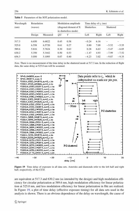
Table 5 Parameters of the SOT polarization model.

Wavelength Retardation Modulation amplitude Time delay of tc (ms)

(nm) (waves) (diagonal element of X Shutterless Shuttered

in shutterless mode)

Design Measured QU V Left Right Left Right

517.3 6.650 6.6822 0.45 0.58 −0.24 6.16 – –

525.0 6.558 6.5720 0.61 0.27 0.80 7.09 −5.52 −5.55

589.6 5.816 5.7624 0.30 0.63 0.28 6.63 −5.47 −6.05

630.2 5.350 5.3442 0.50 0.53 −1.47 4.93 −7.99 −7.52

656.3 5.050 5.1095 0.07 0.40 −4.23 3.02 −9.87 −9.35

Note. There is no measurement of the time delay in the shuttered mode at 517.3 nm. In the reduction of flightdata, the same delay at 525.0 nm will be assumed.

Figure 19 Time delay of exposure in all data sets. Asterisks and diamonds refer to the left half and righthalf, respectively, of the CCD.

are equivalent at 517.3 and 630.2 nm (as intended by the design) and high modulation effi-ciency for circular polarization at 589.6 nm, high modulation efficiency for linear polariza-tion at 525.0 nm, and less modulation efficiency for linear polarization in Hα are realized.In Figure 19, a plot of time delay (effective exposure timing) for all data sets used in theanalysis is shown. There is an obvious dependence of the delay on wavelength, the cause of


Table 6 Telescope matrices and the standard deviation of the fitting residual with the SOT polarizationmodel.

Average T matrix STD deviation of fitting residual

6563 0.9893 −0.0420 −0.0491 0.0018 0.0000 0.0117 0.0296 0.0113

−0.0121 −0.9541 0.0190 0.0072 0.0006 0.0025 0.0005 0.0009

−0.0052 0.0088 0.9764 0.0205 0.0010 0.0011 0.0015 0.0013

−0.0049 −0.0285 −0.0135 1.0070 0.0008 0.0010 0.0019 0.0067

6303 0.9976 0.0101 0.0276 0.0031 0.0000 0.0069 0.0087 0.0062

0.0108 0.9990 0.0145 −0.0025 0.0028 0.0080 0.0022 0.0036

0.0030 0.0131 0.9983 −0.0157 0.0012 0.0021 0.0079 0.0017

−0.0050 0.0437 0.0099 0.9763 0.0015 0.0020 0.0010 0.0086

5896 0.9951 0.0008 0.0730 −0.0006 0.0000 0.0075 0.0107 0.0028

0.0091 0.9970 0.0144 −0.0010 0.0018 0.0046 0.0018 0.0013

0.0013 0.0147 1.0021 −0.0143 0.0018 0.0016 0.0049 0.0019

−0.0099 −0.0178 0.0111 0.9927 0.0010 0.0031 0.0009 0.0103

5250 0.9994 0.0061 0.0141 −0.0082 0.0000 0.0040 0.0148 0.0199

0.0113 0.9996 0.0131 0.0011 0.0032 0.0083 0.0046 0.0027

0.0030 0.0136 1.0031 −0.0169 0.0043 0.0033 0.0137 0.0042

−0.0169 −0.0459 0.0025 0.9931 0.0011 0.0015 0.0020 0.0074

5172 0.9998 0.0007 −0.0296 −0.0458 – – – –

−0.0007 1.0003 0.0077 −0.0077 – – – –

−0.0018 0.0093 0.9863 0.0149 – – – –

−0.0139 0.0543 −0.0246 0.9901 – – – –

Note. Elements in italics exceed the tolerance. Standard deviations are not given for 5172 Å since we haveonly a single measurement for this wavelength.

which is not well understood but is likely due to fabrication error of the waveplate. Residu-als of the fitting (i.e., the difference of Xex and Xfit = DW) averaged in each wavelength forthe telescope matrices are shown in Table 6. The standard deviations of the fitting residualare also shown in the right side of Table 6. Since all elements of the standard deviation otherthan the first column are smaller than the tolerances of the response matrix, we can con-sider that the SOT polarization model developed here well represents the real polarizationresponse matrix of the NFI except for the first column. The elements of the first column willbe determined in orbit, again by using continuum values.

For reference, the polarimeter response matrices provided by the SOT polarization modelare presented in Table 7 for the NFI shutterless IQUV mode, where the telescope matrix isassumed to be unity.

7. Examples of Extended Observing Schemes for the NFI

7.1. Magnetogram (IV Mode)

So far we have been focusing on observations of full Stokes parameters in which a 4 × 4polarimeter response matrix is applicable to retrieve the incident Stokes vector. The NFI can


Table 7 The polarimeter response matrices provided by the SOT polarization model for the NFI shutterlessIQUV mode (Obs_ID = 33, exposure = 100 ms). The telescope matrix is assumed to be unity.

Left-CCD Right-CCD

6563 1.0000 0.8863 0.0000 0.0000 1.0000 0.8863 0.0000 0.0000

0.0000 0.0723 0.0048 0.0000 0.0000 0.0723 −0.0034 0.0000

0.0000 0.0048 −0.0723 0.0000 0.0000 −0.0034 −0.0723 0.0000

0.0000 0.0000 0.0000 −0.4040 0.0000 0.0000 0.0000 −0.4041

6303 1.0000 0.2210 0.0000 0.0000 1.0000 0.2210 0.0000 0.0000

0.0000 0.4958 0.0114 0.0000 0.0000 0.4944 −0.0384 0.0000

0.0000 0.0114 −0.4958 0.0000 0.0000 −0.0384 −0.4944 0.0000

0.0000 0.0000 0.0000 −0.5279 0.0000 0.0000 0.0000 −0.5279

5896 1.0000 0.5389 0.0000 0.0000 1.0000 0.5389 0.0000 0.0000

0.0000 0.2935 −0.0013 0.0000 0.0000 0.2919 −0.0305 0.0000

0.0000 −0.0013 −0.2935 0.0000 0.0000 −0.0305 −0.2919 0.0000

0.0000 0.0000 0.0000 0.6374 0.0000 0.0000 0.0000 0.6338

5250 1.0000 0.0503 0.0000 0.0000 1.0000 0.0503 0.0000 0.0000

0.0000 0.6046 −0.0076 0.0000 0.0000 0.6009 −0.0672 0.0000

0.0000 −0.0076 −0.6046 0.0000 0.0000 −0.0671 −0.6009 0.0000

0.0000 0.0000 0.0000 0.2783 0.0000 0.0000 0.0000 0.2778

5172 1.0000 0.2934 0.0000 0.0000 1.0000 0.2934 0.0000 0.0000

0.0000 0.4498 0.0017 0.0000 0.0000 0.4477 −0.0434 0.0000

0.0000 0.0017 −0.4498 0.0000 0.0000 −0.0434 −0.4477 0.0000

0.0000 0.0000 0.0000 0.5797 0.0000 0.0000 0.0000 0.5790

also take IV information only with two exposures centered at the PMU phases at ±45◦(Figure 20) and the exposure time is selectable in shuttered mode. In practice such a mode,called a “magnetogram,” is useful for making context longitudinal magnetograms at highcadence.

Intensities obtained by the two exposures are given by

I+ = I + cQQ + cV V,

I− = I + cQQ − cV V

and the polarimeter response matrix in this case consists of 4 × 2 elements,

(I ′V ′

)=

(x00 x10 x20 x30

x03 x13 x23 x33

)⎛

⎜⎜⎝

I

Q

U

V

⎞

⎟⎟⎠ ≈

(1 cQ 0 00 0 0 cV

)⎛

⎜⎜⎝

I

Q

U

V

⎞

⎟⎟⎠ .

Here cQ and cV represent Q → I crosstalk and the efficiency of the V measurement,respectively, and are functions of exposure time. Figure 21 shows the plots of cQ and cV

against the exposure time predicted from the SOT polarization model for five NFI wave-lengths. The verification test of such curves was performed by using the FPP and backup


Figure 20 Exposure timing with respect to the PMU modulation phase for the NFI IV mode.

Figure 21 Plots of cQ and cV against the exposure time predicted from the SOT polarization model. Solidcurves are cV (efficiency of V measurement) and dashed curves are cQ (Q → I crosstalk).

(flight spare) unit of the PMU. Figure 21 suggests that there is a preferable exposure time atwhich the Q → I crosstalk becomes negligible for each wavelength.


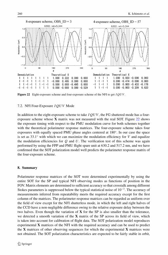
Figure 22 Eight-exposure scheme and four-exposure scheme of the NFI to get IQUV .

7.2. NFI Four-Exposure IQUV Mode

In addition to the eight-exposure scheme to take IQUV , the FG shuttered mode has a four-exposure scheme whose X matrix was not measured with the real SOT. Figure 22 showsthe exposure timing with respect to the PMU modulation curve for both schemes togetherwith the theoretical polarimeter response matrices. The four-exposure scheme takes fourexposures with equally spaced PMU phase angles centered at 180◦. In our case the spaceis set as 33.1◦ with which we can maximize the modulation efficiency for V and equalizethe modulation efficiencies for Q and U . The verification test of this scheme was againperformed by using the FPP and PMU flight spare unit at 630.2 and 517.2 nm, and we haveconfirmed that the SOT polarization model well predicts the polarimeter response matrix ofthe four-exposure scheme.

8. Summary

Polarimeter response matrices of the SOT were determined experimentally by using theentire SOT for the SP and typical NFI observing modes as functions of position in theFOV. Matrix elements are determined to sufficient accuracy so that crosstalk among differentStokes parameters is suppressed below the typical statistical noise of 10−3. The accuracy ofmeasurements inferred from repeatability meets the required accuracy except for the firstcolumn of the matrices. The polarimeter response matrices can be regarded as uniform overthe field of view except for the NFI shutterless mode, in which the left and right halves ofthe CCD have a non-negligible difference owing to the relative exposure delay between thetwo halves. Even though the variation of X for the SP is also smaller than the tolerance,we detected a smooth variation of the X matrix of the SP across its field of view, whichis taken into account for calibration of flight data. The SOT polarization model reproducesexperimental X matrices of the NFI with the required accuracy and can be used to predictthe X matrices of other observing sequences for which the experimental X matrices werenot obtained. The SOT polarization characteristics are expected to be fairly stable in orbit,


whereas the linear retardation of the CLU may have a small offset created during the launchload environment. This possible offset may be checked in real solar data and the X matrixwill be updated if necessary.

Following the successful launch of Hinode on 22 September 2006, the SOT achieved itsfirst light soon after the deployment of the top door of the telescope on 25 October. After theinitial instrument checkout, the SP and the FG began making regular observations of the Sunand are producing excellent Stokes data. We have noticed that the three elements of the firstcolumn of X matrices are very close to zero from the SP and the FG/NFI continuum data.However, we have not yet found any sign implying an offset of the CLU linear retardation(V → QU crosstalk). We need to await further detailed analysis of sunspot data to finalizethis issue.

Polarization calibrations of the SP data are being performed successfully on a regularbasis by using the polarimeter response matrices obtained by HAO. An IDL procedure(fg_pcalx.pro) that provides polarization response matrices for arbitrary NFI products isready and catalogued in the Solar Software (SSW) package.

Acknowledgements The authors are grateful to the late professor T. Kosugi of JAXA/ISAS and to Drs.L. Hill, R. Jayroe, and J. Owens of NASA for continuous support throughout the development of theSOT. The authors also thank Messrs. T. Matsushita and H. Saito of Mitsubishi Electric Corporation andMr. N. Takeyama of Genesia Corporation for extensive thermomechanical analysis of the CLU and alsoMessrs. S. Abe and M. Suzuki of Canon Corporation for indispensable support for the polarization testingof the CLU. One of the authors (KI) also would like to thank Dr. E. West of Marshall Space Flight Center,Dr. R. Chipman of Alabama University, and Dr. Y. Otani of Tokyo University of Agriculture and Technologyfor valuable discussions on the polarization measurements of optical devices in the early phase of the project.Hinode is a Japanese mission developed and launched by ISAS/JAXA, with NAOJ as domestic partner andNASA and STFC (UK) as international partners. It is operated by these agencies in cooperation with ESAand NSC (Norway).

References

Elmore, D.F.: 1990, A polarization calibration technique for the advanced stokes polarimeter. NCAR Tech-nical Note NCAR/TN-355+STR, NCAR, Boulder, Colorado.

Guimond, S., Elmore, D.: 2004, OE Mag. 4(5), 26.Ichimoto, K., Tsuneta, S., Suematsu, Y., Shimizu, T., Otsubo, M., Kato, Y., et al.: 2004, In: Mather, J.C. (ed.)

Optical, Infrared, and Millimeter Space Telescopes, Proc. SPIE 5487, 1142.Ichimoto, K., the Solar-B Team: 2005, J. Korean Astron. Soc. 38, 307.Ichimoto, K., Shinoda, K., Yamamoto, T., Kiyohara, J.: 2006, Publ. Natl. Astron. Obs. Japan 8, 11.Kosugi, T., Matsuzaki, K., Sakao, T., Shimizu, T., Sone, Y., Tachikawa, S., et al.: 2007, Solar Phys. 243, 3.Shimizu, T.: 2004, In: Sakurai, T., Sekii, T. (eds.) The Solar-B Mission and the Forefront of Solar Physics

CS-325, Astron. Soc. Pac., San Francisco, 3.Shimizu, T., Nagata, S., Edwards, C., Tarbell, T., Kashiwagi, Y., Kodeki, K., et al.: 2004, In: Mather, J.C.

(ed.) Optical, Infrared, and Millimeter Space Telescopes, Proc. SPIE 5487, 1199.Shimizu, T., Nagata, S., Tsuneta, S., Tarbell, T., Edwards, C., Shine, R., et al.: 2008, Solar Phys. in press.Skumanich, A., Lites, B.W.: 1997, Astrophys. J. Suppl. 110, 357.Suematsu, Y., Tsuneta, S., Ichimoto, K., Shimizu, T., Otsubo, M., Katsukawa, Y., et al.: 2008, Solar Phys.

in press.Tarbell, T.D., et al.: 2008, Solar Phys. to be submitted.Tsuneta, S., Ichimoto, K., Katsukawa, Y., Shimizu, T., Otsubo, M., Nagata, S., et al.: 2008, Solar Phys.

in press.

polarization calibration of the solar optical telescope ...6265/datastream... · polarization...

Documents