PHYSICAL REVIEW A 93, 063827 (2016)

Polariton states in circuit QED for electromagnetically induced transparency

Xiu Gu,1,2 Sai-Nan Huai,1 Franco Nori,2,3 and Yu-xi Liu1,2,4,*

1Institute of Microelectronics, Tsinghua University, Beijing 100084, China2CEMS, RIKEN, Saitama 351-0198, Japan

3Department of Physics, The University of Michigan, Ann Arbor, Michigan 48109-1040, USA4Tsinghua National Laboratory for Information Science and Technology (TNList), Beijing 100084, China

(Received 3 February 2016; published 14 June 2016)

Electromagnetically induced transparency (EIT) has been extensively studied in various systems. However, itis not easy to observe in superconducting quantum circuits (SQCs) because the Rabi frequency of the strong-controlling field corresponding to EIT is limited by the decay rates of the SQCs. Here, we show that EIT can beachieved by engineering decay rates in a superconducting circuit QED system through a classical driving fieldon the qubit. Without such a driving field, the dressed states of the system, describing a superconducting qubitcoupled to a cavity field, are approximately product states of the cavity and qubit states in the large-detuningregime. However, the driving field can strongly mix these dressed states. These doubly dressed states, here calledpolariton states, are formed by the driving field and dressed states, and are a mixture of light and matter. Theweights of the qubit and cavity field in the polariton states can now be tuned by the driving field, and thus thedecay rates of the polariton states can be changed. We choose the three lowest-energy polariton states with a�-type transition in such a driven circuit QED system, and demonstrate how EIT and Autler-Townes splittingcan be realized in this compound system. We believe that this study will be helpful for EIT experiments usingSQCs.

DOI: 10.1103/PhysRevA.93.063827

I. INTRODUCTION

Since electromagnetically induced transparency (EIT) wasproposed [1], it has been extensively explored in variouscontexts [2–5] using three-level systems. The main featureof EIT is that the absorption of a weak probe field in a mediumis reduced because of the presence of a strong-control field.EIT can be used to control the propagation of the weak fieldthrough the medium. It can also be used to greatly enhance thenonlinear susceptibility in the induced transparency region,and thus to generate a strong photon-photon Kerr interaction.Strong photon-photon Kerr interactions have been studied torealize quantum logic operations such as controlled phase gates[6], quantum Fredkin gates [7], and conditional phase switches[8] for photon-based quantum information processing. More-over, Kerr interactions can be employed to realize quantumnondemolition detection of photons [9].

Recent studies show that superconducting quantum circuits(SQCs) are one of the best candidates for quantum infor-mation processing [10–14]. Meanwhile, these artificial atoms[10,11,13,15,16] have been employed to study quantum opticsand atomic physics in the microwave domain. For example,several studies [17–21] have explored population trapping anddark states in three-level SQCs. EIT was also theoreticallystudied for probing the decoherence of a superconductingflux qubit [22,23] via a third auxiliary state. How to realizeEIT using SQCs has also been theoretically studied usingseveral different setups [24–26]. Experimentalists showedAutler-Townes splitting (ATS) [27] using various three-levelSQCs [21,28–36]. However, EIT experiments are difficult tomake using superconducting circuits. The main obstacle is thatthe decay rates of the three-level system and the strength of the

*yuxiliu@mail.tsinghua.edu.cn

Rabi frequency corresponding to the controlling field cannotsatisfy the condition for realizing EIT [26,37,38].

It is well known that EIT [1] is mainly caused by Fanointerference [39], while ATS [27] is due to the driving-field-induced shift of the transition frequency. Although themechanisms of EIT and ATS are very different, they are noteasy to discern from experimental observations since both ofthem exhibit a dip in the absorption spectrum of the weak probefield. Theoretically, there is a threshold value [26,37,38] todistinguish EIT from ATS. This threshold value is determinedby two decay rates of the three-level system [26,37,38]. Whenthe strength of the Rabi frequency of the strong-controllingfield is smaller than this value, EIT occurs, otherwise, it isATS. Experimentally, the data should be analyzed by virtueof the Akaike information criterion [38]. The transition fromEIT to ATS has been experimentally demonstrated in coupledwhispering-gallery-mode optical resonators [40].

Here, instead of three-level superconducting quantumcircuits [22–26], we study EIT and the transition from EIT toATS using a driven two-level circuit QED system [12], wherea superconducting qubit is coupled to a single-mode cavityfield and driven by a classical field. The three-level systemused to study EIT is constructed by the three lowest-energymixed polariton states, formed by the driving field and thedressed states of the circuit QED system. The polariton statesare hybridizations of microwave photon and qubit states. Thus,the decays of the polariton states are determined by the decaysof both the cavity field and the superconducting qubit.

The eigenstates of the circuit QED system are dressedstates of the cavity field and the superconducting qubit. Thesestates can be approximately reduced to product states of theuncoupled cavity field and qubit states when the frequenciesof the cavity field and the superconducting qubit are largelydetuned. In this case, the qubit acquires a small frequencyshift due to the microwave field and the Purcell [41] enhanced

2469-9926/2016/93(6)/063827(12) 063827-1 ©2016 American Physical Society

XIU GU, SAI-NAN HUAI, FRANCO NORI, AND YU-XI LIU PHYSICAL REVIEW A 93, 063827 (2016)

spontaneous decay rate [42] is obtained. Therefore, when thedetuning between the cavity field and the qubit is changedfrom zero to a finite value, the decay rates of the eigenstatesof the circuit QED system can also be changed. However,such tunable decay is not easy to be realized when the sampleis fabricated. Thus, we introduce a classical driving field tofurther mix the dressed states. We refer to these doubly dressedstates as polariton states. In solid-state physics, polaritons areelementary excitations that are half light and half matter. In oursystem, the mixture of the driving field and the dressed statesinherits both atomic and photonic properties. The weights ofthe photon and qubit states in polariton states can be tuned bythe driving field, and thus the decay of the polariton states canbe controlled. Such polariton states were studied in order toimplement an impedance-matched � system [43–45], wherethe two decay rates from the highest-energy level to the twolowest-energy levels are identical. However, in our study, weneed to engineer different decay rates of the three-level �

system so that the condition to realize EIT and ATS can besatisfied. In contrast to the study [24], an extra driving field onthe qubit is introduced to modify the decay rates of the systemstudied.

The paper is organized as follows. In Sec. II, we describe amodel Hamiltonian and discuss how the transition frequenciescan be tuned by the driving field. In Sec. III, we study theselection rules and how to control decay rates of polaritonstates by changing the driving field. In Sec. IV, we studya three-level polariton system to implement EIT and ATS,and the threshold value to discern EIT and ATS is given.Numerical simulations with possible experimental parametersare presented. Finally, further discussions and a summary arepresented in Sec. V.

II. THEORETICAL MODEL AND POLARITON STATES

In this section, we derive polariton states from the modelHamiltonian and then discuss how decay rates of the polaritonstates can be adjusted by an externally applied classical field.

A. Hamiltonian

As schematically shown in Fig. 1, we study a supercon-ducting two-level system (a qubit system) which is coupledto a quantized single-mode microwave field and also drivenby a classical microwave field. For concreteness, we assumethat such qubit system is a three-Josephson-junction flux qubitcircuit. The interaction between the qubit and the single-modecavity field is described by the well-known Jaynes-Cummings

qubi

t driv

e

FIG. 1. A driven qubit coupled to a resonator mode. Here,{|g〉,|e〉} are the ground and excited states of the qubit, g is thecoupling strength between the qubit and the cavity field, and γq (γc)is the decay rate of the qubit (cavity field).

model [46,47]. Thus, the model Hamiltonian of the drivencircuit QED system can be written as

HS = �

2ωqσz + �ωr

(a†a + 1

2

)+ �g

(a†σ− + aσ+

)

+ �[�σ− exp (iωdt) + �∗σ+ exp (−iωdt)]. (1)

The first line of Eq. (1) is the Jaynes-Cummings Hamiltonian,which describes the interaction between the qubit system andthe single-mode cavity field with coupling strength g. Here,ωq and ωr denote the frequencies of the qubit and single-modecavity field, respectively. Also, a is the annihilation operatorof the cavity field and σ− is the ladder operator of the qubit.The second line of Eq. (1) describes the interaction betweenthe qubit and the classical driving field. The parameter �

represents the interaction strength or Rabi frequency betweenthe qubit and the classical field with frequency ωd . Withoutloss of generality, hereafter we assume that � is a real number.

To remove the time-dependent factors, we transform theHamiltonian HS , given in Eq. (1), into a rotating referenceframe by the unitary transformation

U = exp[−iωd (σz/2 + a†a)t], (2)

so that we can obtain the following effective Hamiltonian:

HS = �

2ωqσz + �ωr

(a†a + 1

2

)+ �g(a†σ− + aσ+)

+ �[�σ− + �σ+], (3)

with the detunings ωq = ωq − ωd , ωr = ωr − ωd , and � =ωr − ωq .

B. Eigenvalues and eigenstates for � = 0

For completeness, we first briefly discuss the eigenstatesand eigenvalues when the classical driving field is not appliedto the qubit. In this case, � = 0, and the eigenstates of Eq. (3),for the Jaynes-Cummings Hamiltonian of the qubit and thesingle-mode cavity field, are

|+,n〉 = cosθn

2|e,n〉 + sin

θn

2|g,n + 1〉, (4)

|−,n〉 = − sinθn

2|e,n〉 + cos

θn

2|g,n + 1〉, (5)

which mix the qubit states with the states of a single-modecavity field. Here, tan θn = −2g

√n + 1/�. We note that

|e,n〉 ≡ |e〉|n〉 (|g,n〉 ≡ |g〉|n〉) denote that the qubit is in theexcited |e〉 (ground |g〉) state and the single-mode cavity fieldis in the state |n〉. The states expressed in Eqs. (4) and (5) areusually called dressed states. Note that we do not distinguishthe dressed states in the rotating reference frame from those inthe original laboratory frame. The eigenvalues correspondingto Eqs. (4) and (5) are

E±,n = �ωr

(n + 1

2

)± �

2

√�2 + 4g2(n + 1). (6)

From Eqs. (4) and (5), it is clear that the eigenenergiesof the Jaynes-Cummings model change with the detuning �

between the qubit and the single-mode cavity field. Whenthe detuning is very large, the dressed states are approachingeither bare qubit states or the states of the single-mode cavity

063827-2

POLARITON STATES IN CIRCUIT QED FOR . . . PHYSICAL REVIEW A 93, 063827 (2016)

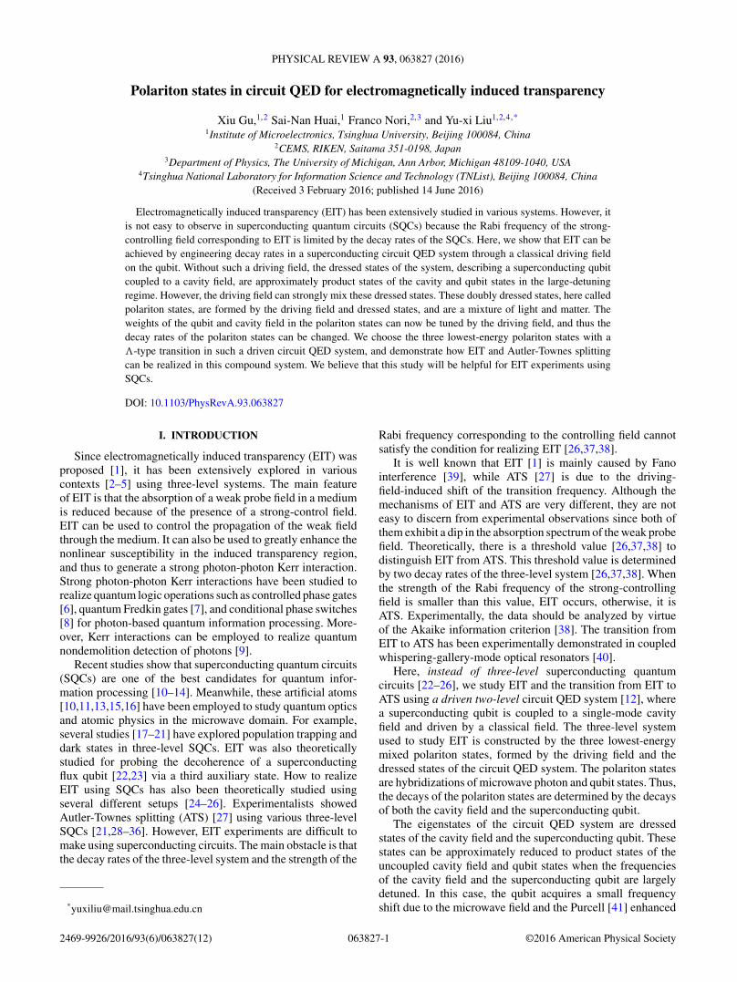
FIG. 2. A schematic energy diagram for the Jaynes-Cummingsmodel vs the detuning between the qubit and cavity field in the rotatingframe. The eigenstates are denoted by |±,n〉. In the large-detuningregime, the coupled states |±,n〉 are approaching the bare qubit andphoton states. Here, � = ωr − ωq . The nesting regime, defined byω|g,0〉 � ω|e,0〉 < ω|e,1〉 � ω|g,1〉, as in Refs. [43–45], is between thetwo points linked by a line with two arrows. The frequency of thedriving field ωd sets the boundary of the nesting regime. The lowerlimit is at ω|e,1〉 = ω|g,1〉, where ωd = ωq − 3χ . The upper limit isat ω|g,0〉 = ω|e,0〉, where ωd = ωq − χ . Here, χ = g2/�, with g thecoupling strength between the qubit and cavity field. We note thatwhen the zero-point fluctuation of the cavity field is taken intoaccount, the energy of the ground state |g〉|0〉 is �/2.

field. That is, they are almost decoupled from each other. Theeigenenergies in Eq. (6) are shown as a function of the detuning� in Fig. 2, which clearly shows that the qubit and the cavityfield are decoupled from each other when � becomes verylarge. Figure 2 also shows that there are some degeneracypoints when � takes a particular value, e.g., Eg,0 = E−,0 andE+,0 = E−,1, which will be further discussed in the followingin the large-detuning case.

In the large-detuning case, i.e., g � |�|, Eqs. (4) and (5)can be approximately written as

|+,n〉 ≈ |g,n + 1〉 − g

�

√n + 1|e,n〉, (7)

|−,n〉 ≈ |e,n〉 + g

�

√n + 1|g,n + 1〉, (8)

where we assume � > 0 for convenience in the followingdiscussions. We now focus on the five lowest eigenstates of theJaynes-Cummings model, i.e., the ground state |g,0〉 and thefour dressed states |±,0〉 and |±,1〉. To simplify the analysis,we first omit the first order of g/�. In this case, the four dressedstates can be approximately written as |−,0〉 ≈ |e,0〉, |+,0〉 ≈|g,1〉, |−,1〉 ≈ |e,1〉, and |+,1〉 ≈ |g,2〉, which correspond tothe eigenfrequencies E±,n/� given by

ω|g,n〉 ≈ n(ωr + χ ) + �

2, (9)

ω|e,n〉 ≈ ωq − χ + n(ωr − χ ) + �

2, (10)

where χ = g2/� is the dispersive frequency shift. FromEqs. (9) and (10), we can approximately obtain ω|e,0〉 = ω|g,0〉at ωq = χ , and ω|e,1〉 = ω|g,1〉 at ωq = 3χ . Thus, to operatein the so-called nesting regime [43–45], where ω|g,0〉 <

ω|e,0〉 < ω|e,1〉 < ω|g,1〉, that is, Eg,0 < E−,0 < E−,1 < E+,0,the frequency ωd of the driving field must satisfy the conditionωq − 3χ < ωd < ωq − χ .

C. Eigenvalues and eigenstates for � �= 0

When a classical driving field is applied to the qubit, i.e.,� �= 0, it will induce transitions between different states of|±,n〉. Thus, the classical driving field lifts the degeneraciesand strongly mixes the states |±,n〉 with the states |±,n + 1〉.That is, the dressed states in Eqs. (4) and (5) are mixed againby the classical field. We refer to these new states as polaritonstates because they inherit both atomic and photonic properties.Below, we will mainly focus on the large-detuning regime.

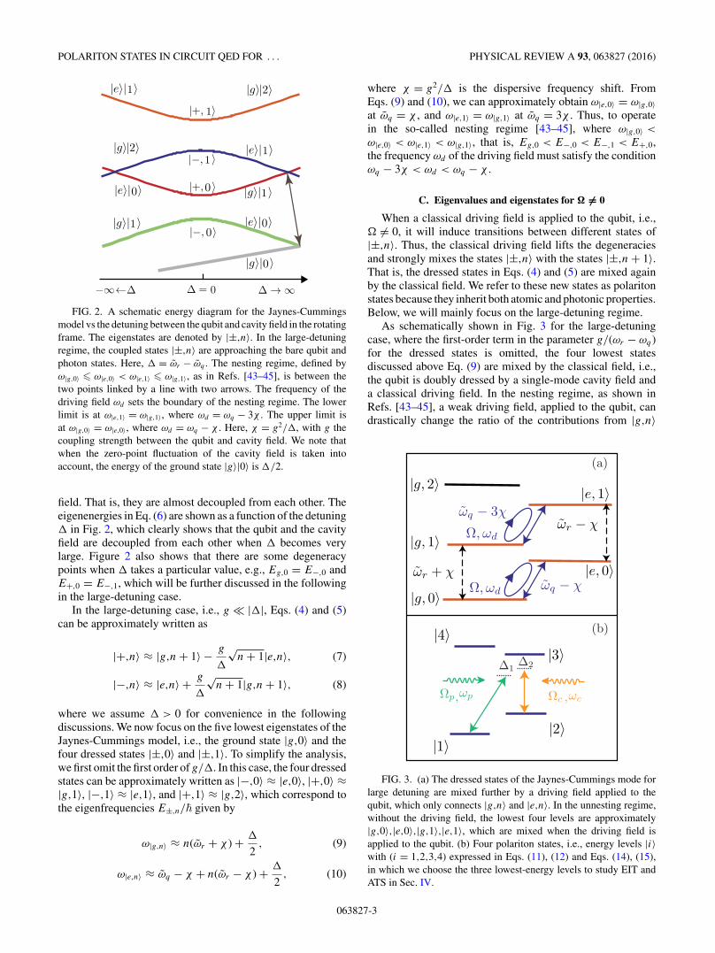
As schematically shown in Fig. 3 for the large-detuningcase, where the first-order term in the parameter g/(ωr − ωq)for the dressed states is omitted, the four lowest statesdiscussed above Eq. (9) are mixed by the classical field, i.e.,the qubit is doubly dressed by a single-mode cavity field anda classical driving field. In the nesting regime, as shown inRefs. [43–45], a weak driving field, applied to the qubit, candrastically change the ratio of the contributions from |g,n〉

(a)

(b)

FIG. 3. (a) The dressed states of the Jaynes-Cummings mode forlarge detuning are mixed further by a driving field applied to thequbit, which only connects |g,n〉 and |e,n〉. In the unnesting regime,without the driving field, the lowest four levels are approximately|g,0〉,|e,0〉,|g,1〉,|e,1〉, which are mixed when the driving field isapplied to the qubit. (b) Four polariton states, i.e., energy levels |i〉with (i = 1,2,3,4) expressed in Eqs. (11), (12) and Eqs. (14), (15),in which we choose the three lowest-energy levels to study EIT andATS in Sec. IV.

063827-3

XIU GU, SAI-NAN HUAI, FRANCO NORI, AND YU-XI LIU PHYSICAL REVIEW A 93, 063827 (2016)

and |e,n〉 to the final polariton states. This is in contrast tothe unnesting case, where the external qubit drive has noappreciable effect on the system, as the following analysisshows.

The classical qubit field only induces transitions betweenthe states |g,n〉 and |e,n〉. Thus, it can only mix the state|g,0〉 with |±,0〉, or mix states |±,n〉 with states |±,n + 1〉. Inthe large-detuning case, the states |g,0〉 and |−,0〉 ≈ |e,0〉 areseparated by the energy level spacing ωq − χ , when the drivingfield is not applied. Thus, in the lower boundary of the nestingregime, when the frequency of the driving field satisfies thecondition ωd = ωq − χ , the driving field induces transitionsbetween the states |−,0〉 ≈ |e,0〉 and |g,0〉 and strongly mixthese two states. These mixed states form new doubly dressedeigenstates, the so-called polariton states,

|1〉 = − sinθl

2|e,0〉 + cos

θl

2|g,0〉, (11)

|2〉 = cosθl

2|e,0〉 + sin

θl

2|g,0〉. (12)

Here, tan θl = 2�/(ωq − χ). The transition frequencybetween the state |1〉 and the state |2〉 is given by

ω21 =√

(ωq − χ )2 + 4�2, (13)

with ωij = ωi − ωj . Likewise, the states |+,0〉 ≈ |g,1〉 and|−,1〉 ≈ |e,1〉, with original level spacing ωq − 3χ , can bemixed by the qubit driving field at the upper boundary ofthe nesting regime when ωd = ωq − 3χ . Thus, these polaritonstates (i.e., eigenstates) can be given by

|3〉 = − sinθu

2|g,1〉 + cos

θu

2|e,1〉, (14)

|4〉 = cosθu

2|g,1〉 + sin

θu

2|e,1〉, (15)

with tan θu = 2�/(−ωq + 3χ ). The energy splitting between|4〉 and |3〉 becomes

ω43 =√

(ωq − 3χ )2 + 4�2. (16)

As schematically shown in Fig. 2(b), below we will choose{|1〉,|2〉,|3〉} to form a three-level system. The transitionfrequency ω31 between the state |3〉 and the state |1〉 is givenby

ω31 = ωr − 12 (ω43 + ω21). (17)

In Fig. 4, transition frequencies are plotted as functions ofthe qubit driving frequency ωd and strength � in the rotatingreference frame. Here we use the exact solution of Eq. (3) in thenumerical calculation. In other words, without large-dispersiveapproximation, each new eigenstate |i〉 is the superposition offive states: |g,0〉, |e,0〉, |g,1〉, |e,1〉, and |g,2〉. Figure 4(a)shows the trend of ω21 and ω43, and they are consistent withEqs. (13) and (16). First we discuss the � = 0 case, in whichthe driving field is not applied. The lowest two energy levels |1〉and |2〉 are composed of |g,0〉 and |e,0〉. The degeneracy point,where ω21 = 0, is set by ω|e,0〉 = ω|g,0〉, i.e., ωd = ωq − χ ,which is the upper boundary of the nesting regime. Likewise,the states |4〉 and |3〉 are superpositions of the states |g,1〉 and|e,1〉. The degeneracy point is set by ω|e,1〉 = ω|g,1〉, i.e., ωd =

ωd/2π (GHz)

Ω/2

π (M

Hz)

ωij/2

π (

GH

z)

40200

0.1

04.95

0.2

4.85

(b)

ωij/2

π (

GH

z)

ω d/2

π

Ω/2π (MHz)

4.954.85

4.85020

5.05

40

5.25 ω31

ω32

(a)

ω21 ω

43

(GH

z)

FIG. 4. Transition frequencies ωij vs both the frequency ωd andthe strength � of the driving field in the rotating reference frame.Here, ωij = ωi − ωj . The parameters used here are ωq/2π = 5 GHz,ωr/2π = 10 GHz, g/2π = 500 MHz, and χ/2π = 50 MHz. (a) TwoV-shaped surfaces with the minimum values at ωd/2π = 4.95 andωd/2π = 4.85 GHz represent ω21 and ω43, respectively. (b) The uppersurface represents ω31 and the lower one represents ω32.

ωq − 3χ , which is the lower boundary of the nesting regime.We note that ω43 = ω21 in the middle of nesting regime whenωq = 2χ . It is clear that the frequency ωd of the driving fielddetermines the onset of the nesting regime. When the drivingfield is applied to the qubit, i.e., � �= 0, these degeneracies arelifted. The larger strength � is, the larger ω21 and ω43 are.

We also show how the frequency and the strength of thedriving field affect the transition frequencies ω31 and ω32

in Fig. 4(b). It clearly shows that the upper surface for thetransition frequency ω31 approaches that of ω32 when the states|2〉 and |1〉 are degenerate. When the driving strength is small,ω31 and ω21 are mainly determined by ωr and χ . However, χ ,which is determined by g and � in the large-dispersive regime,can be enhanced by the presence of the higher excited states[42–45].

III. TRANSITION RULES AND TUNABLE DECAY RATES

A. Transition rules between polariton states

Since the polariton states, formed by the cavity field, drivingfield, and the qubit, are mixed photon and qubit states, we caninduce transitions between two of these new states by applyingadditional classical fields to either the qubit or the cavity field.Hereafter we refer to these classical fields as the external fields,to avoid confusion with the classical driving field applied tothe qubit with coupling strength �. The transition selection

063827-4

POLARITON STATES IN CIRCUIT QED FOR . . . PHYSICAL REVIEW A 93, 063827 (2016)

rule between these polariton states depends on the manner inwhich the external field is applied. For example, the transitionsbetween the state |e,n〉 and |g,n〉 can be induced when theexternal field is applied to the qubit. However, those transitionsare forbidden when the external field is applied to the cavityfield. In contrast, the transitions between the state |l,n〉 and|l,n − 1〉, with l = e or l = g, can be induced by the externalfield applied to the cavity field. However, these transitions areforbidden if the external field is applied to the qubit. Therefore,the transition matrix elements between two polariton states canbe tuned by varying the applied external field.

When the external field is applied to the qubit, the transitionmatrix elements are denoted by

Qij = |〈i|σ−|j 〉|. (18)

Similarly, when the external field is applied to the cavity field,the transition matrix elements are defined as

Cij = |〈i|a|j 〉|. (19)

Here, |i〉 and |j 〉 denote the new polariton states, e.g., the statesin Eqs. (11), (12) and Eqs. (14), (15) in the large-detuning case.The transition elements between two of the states in Eqs. (11),(12) and (14) can be written as

C32 =∣∣∣∣cos

(θu + θl

2

)∣∣∣∣, (20)

C31 =∣∣∣∣sin

(θu + θl

2

)∣∣∣∣, (21)

Q21 = cos2

(θl

2

), (22)

Q31 = Q32 = C21 = 0. (23)

Equations (20)–(23) clearly show that transitions betweenthe states |3〉 and |2〉 or between the states |3〉 and |1〉 arecontrolled by the driving field applied to the cavity field.However, the transition between the states |2〉 and |1〉 isdominated by the driving field applied to the qubit. Figure 5numerically shows how the matrix elements change withthe frequency ωd and the strength � of the driving field.The nonzero values for Q32, Q31, and C21, as shown inFigs. 4(b), 4(d), and 4(f), are limited by the first order of g/�

which we omitted in Eqs. (7) and (8). Moreover, the behaviorof Q32, Q31, and C21 is identical to C32, C31, and Q21. So, in thefollowing analysis, we focus on the dominant matrix elementsin the different parameter ranges.

(i) Outside the nesting regime, where ωd < ωq − 3χ , thedriving field applied to the qubit has no appreciable affects, andwe have |1〉 ≈ |g,0〉, |2〉 ≈ |e,0〉, |3〉 ≈ |g,1〉, and |4〉 ≈ |e,1〉.As shown in Figs. 4(a), 4(c), and 4(e), C32 ≈ 0, C31 ≈Q21 ≈1.The lowest three energy levels can be formed into a three-levelsystem with V-type transitions. That is, one external field isapplied to the cavity field to induce the transition between thestates |3〉 and |1〉, while the other one is applied to the qubit toinduce the transition between the states |2〉 and |1〉.

(ii) In the nesting regime, where ωq − 3χ < ωd < ωq − χ ,the driving field applied to the qubit drastically changes theproperties of the polariton states. We take C32, shown inFig. 5(a), as an example. The saddle shape of C32 is consistent

(a) C32

0

0.5

4.95 40

1

204.850

(b) Q32

0

0.05

4.95 40

0.1

204.850

(c) C31

0

0.5

4.95 40

1

204.850

(d) Q31

0

0.05

4.95 40

0.1

204.850

(f) C21

ωd/2π (GHz) Ω/2π (MHz)

0

0.05

4.95 40

0.1

204.850

ωd/2π (GHz) Ω/2π (MHz)

(e) Q

21

0

0.5

4.95 40

1

204.850

FIG. 5. Moduli of the transition matrix elements between the state|i〉 and the state |j〉 vs both the strength � and the frequency ωd ofthe driving field. Qij denotes the transition matrix elements betweenthe states |i〉 and |j〉, induced by an external field applied to the qubit,while Cij is the one induced by an external field applied to the cavityfield. The sharp change in Qij and Cij occurs at the boundary ofthe nesting regime; when � = 0, this occurs when ωq − 3χ < ωd <

ωq − χ . Note that the nonzero coupling in (b), (d), and (e) is limitedby the first order of g/�, which we omit in the theoretical analysis.The parameters are the same as in Fig. 4. Here, the states |i〉 fornumerical calculations of the transition matrix elements are given bythe exact eigenstates of Eq. (3).

with the boundary of the nesting regime. We first discussthe weak-driving case, i.e., � ≈ 0. In this case, we have|1〉 ≈ |g,0〉, |2〉 ≈ |e,0〉, |3〉 ≈ |g,1〉, and |4〉 ≈ |e,1〉, and thisis the same with (i). The first sharp transition of C32 occursat ω|e,1〉 = ω|g,0〉, when ωd = ωq − 3χ , and then the state |3〉is changed to |e,1〉 with the change of the driving frequencyωd through entering the nesting regime, where the transitionC32, due to the driving field applied to the cavity, has a suddenjump from 0 to the finite value. Then, when changing thefrequency ωd of the driving field, when ωd = ωq − χ , thestate |2〉 changes from |e,0〉 to |g,0〉, while the state |3〉 can beapproximated to |3〉 ≈ |e,1〉, and hence the transition matrixelement C32 drops sharply. This is the same for the reversetrend of the transition matrix element C31. It is understandablethat for the transition between the states |2〉 and |1〉, the sharpturning point is at the upper boundary, where ω|e,0〉 = ω|g,0〉. In

063827-5

XIU GU, SAI-NAN HUAI, FRANCO NORI, AND YU-XI LIU PHYSICAL REVIEW A 93, 063827 (2016)

this condition, we have C32 ≈ 1, Q21 ≈ 1, and C31 ≈ 0 whenthe driving field is rather weak, i.e., � ≈ 0, and the systembehaves like a �-type transition where the states |2〉 and |1〉are linked by the external field applied to the qubit, while thestates |3〉 and |2〉 are linked by the external field applied to thecavity field.

(iii) In the nesting regime, when � �= 0, with the increasingof the strength � of the driving field applied to the qubit, thestate |3〉 becomes a mixing of the states |g,1〉 and |e,1〉, and thestate |2〉 becomes a mix of the states |g,0〉 and |e,0〉. Thus,the matrix element C32 decreases gradually when increasingthe driving strength �. Likewise, the matrix element C31

increases when increasing the driving strength �. If twoexternal driving fields are applied to the cavity field, thentwo transitions between the states |3〉 and |2〉, and between thestates |3〉 and |1〉, are induced; in this case, we can constructa three-level system with the �-type transition, which will beused to study EIT and ATS in the following section. If anotherexternal field is applied to the qubit, then the transition betweenthe states |2〉 and |1〉 can be induced, and the three-levelsystem now possesses cyclic transitions, or a �-type [48,49]transition. For natural atoms, �-type transitions do not existbecause the dipole operator possesses odd parity; it can onlyconnect states with different parities.

EIT only occurs in three-level systems with �-type tran-sition or three-level systems with the upper driven �-typetransition [37,50]. In the next section, we will focus on athree-level system with �-type transition and study how EITand ATS can be tuned by changing the driving field applied tothe qubit.

B. Tunable decay rates of mixed polariton states

To study EIT, we first study how the classical driving fieldcan be used to adjust the decay rates of the mixed polaritonstates by varying its amplitude and the frequency. The mainidea is to change the ratio of how the cavity field or qubitcontributes to the final mixture. If the cavity field and thequbit have different decay rates, then the decay rates of thepolariton states vary with the weights of the cavity field branchand the qubit branch in the polariton states. To discuss thedecay rates of the polariton states, let us assume that theenvironment interacting with the system can be described bybosonic operators. Then the Hamiltonian of the whole system,including the environment, can be written as

H ′ = HS + HE + HI , (24)

where the Hamiltonian HS is given in Eq. (1). The freeHamiltonian HE in Eq. (24) of the environment is given by

HE = �

∫dωωb†(ω)b(ω) + �

∫dω′ω′c†(ω′)c(ω′). (25)

The interaction Hamiltonian HI in Eq. (24) between the systemand the environment is given by

HI = �

[∫dωK(ω)b†(ω)a + H.c.

]

+[∫

dω′η(ω′)c†(ω′)σ− + H.c.

]. (26)

We have assumed that the environment of the cavity field isindependent of that of the qubit. Here, b†(ω) and c†(ω′) denotethe creation operators of the environmental bosonic modes ofthe cavity field and the qubit, respectively. For simplicity, wefurther assume that the spectrum of the environment is flat,that is, both K(ω) and η(ω′) are independent of frequency. Inthis case, we can introduce the first Markov approximation,

K(ω) =√

γc/2π, (27)

η(ω′) = √

γq/2π. (28)

In the polariton basis, the operators a and σ− of the cavityfield and the qubit can be expressed as

a =∑ij

〈i|a|j 〉σij , (29)

σ− =∑lm

〈l|σ−|m〉σlm, (30)

where |i〉, |j 〉, |l〉, and |m〉 denote mixed polariton states, whichcan be expressed by either the mixture of Eqs. (4) and (5), forthe general case, or the mixture of Eqs. (7) and (8), for thelarge-detuning case. Here, σij = |i〉〈j |. In the basis of themixed polariton states, the interaction Hamiltonian HI can berewritten as

HI = �

∫dω

∑ij

[√γ c

ij /2πb†(ω)σij + H.c.]

+ �

∫dω′

⎡⎣∑

ij

√γ

q

ij /2πc†(ω′)σij + H.c.

⎤⎦, (31)

with γ cij = γc|〈i|a†|j 〉|2 and γ

q

ij = γq |〈i|σ+|j 〉|2. Thus, thetotal decay rate γij from one mixed polariton state |i〉 to anotherone |j 〉 transition is given by

γij = γ cij + γ

q

ij = γc|〈i|a†|j 〉|2 + γq |〈i|σ+|j 〉|2. (32)

In the large-detuning regime, where the cavity field and thequbit have very different frequencies, the decay rates, fromone upper state to another lower state, expressed from Eq. (11)to Eq. (14), can be approximately given by

γ31 = γc sin2

(θu + θl

2

), (33)

γ32 = γc cos2

(θu + θl

2

), (34)

γ21 = γq cos4

(θl

2

). (35)

In the large-detuning regime, we also find γ31 ≈ γ42, γ32 ≈ γ41,γ c

ii = γc|〈i|a†|i〉|2 ≈ 0, and γ c21 = γ

q

43 ≈ 0.Figure. 6 shows how the decay rates γij change with the

frequency and strength of the driving field, plotted for themixed polariton states. The decay rates are proportional tothe square of the transition matrix elements. Therefore theyhave similar features for the dependence on the frequency andstrength of the driving field. This can be seen by comparing

063827-6

POLARITON STATES IN CIRCUIT QED FOR . . . PHYSICAL REVIEW A 93, 063827 (2016)

40

(a) γ31

(MHz)

0

10

4.95

20

204.85 0

(b) γ32

(MHz)

0

10

4.95 40

20

204.85 0

Γ31

(MHz)(c)

19.5

20

4.95 40

20.5

204.85 0

ωd/2π (GHz) Ω/2π (MHz)

(d)γ21

(MHz)

0

0.5

4.95 40

1

204.85 0

FIG. 6. Decay rates γij vs both the frequency and strength of thedriving field. Here, we set 31 = γ31 + γ32 ≈ γc. We have chosenγq/2π = 1 MHz, γc/2π = 20 MHz.

Fig. 5 with Fig. 6. We define the total decay rate of the state |3〉as 31 = γ31 + γ32. We find that 31 is hardly influenced bythe driving field in the large-detuning case, except that thereis a slight jump at the lower bound of the nesting regime.This is consistent with Eqs. (33) and (34), i.e., 31 ≈ γc. In thenesting regime, the decay rates γ31 and γ32 change significantlywhen varying �; the decay rate γ21 is slightly decreasedwhen � is increased. We find γ31 = γ32 when � is taken asa particular value. This is an impedance-matching condition[43], in which the two decay rates from the highest-energylevel |3〉 to the two lowest-energy levels |1〉 and |2〉 are thesame, and microwave photons are down converted efficientlythrough Raman transitions due to impedance matching [45].Instead of using the impedance-matching condition, below wemainly study how EIT can occur in a chosen three-level systemby using proper decay rates through adjusting the driving field.

IV. ELECTROMAGNETICALLY INDUCEDTRANSPARENCY AND AUTLER-TOWNES SPLITTING

A. Linear response of a � system

We now study the EIT effect in a � configuration atominteracting with two classical fields, as shown in Fig. 3(b). Thetransition between the states |3〉 and |2〉 is linked by a strongexternal field with frequency ωc, hereafter called the controlfield. A probe field with frequency ωp is applied to inducethe transition between the states |3〉 and |1〉. The presence ofa strong driving field dramatically modifies the response ofthe system to the weak probe field. As shown, for example,in Ref. [5], the response of the probe field is analyzed using asemiclassical approach through the master equation.

The master equation for the reduced density matrix operatorρ of the three-level system can be given by [5]

ρ = − i

�[Hint,ρ] + γ31

2[2σ13ρσ31 − σ31σ13ρ − ρσ31σ13]

+ γ32

2[2σ23ρσ32 − σ32σ23ρ − ρσ32σ23]

+ γ21

2[2σ12ρσ21 − σ21σ12ρ − ρσ21σ12]. (36)

Here, we have neglected the energy-conserving dephasingprocesses of the three-level system. Also, γij is the spontaneousdecay rate from |i〉 to |j 〉, which coincides with Eq. (32).Note that compared to Ref. [5], we have taken into accountthe spontaneous decay from |2〉 to |1〉. For natural atoms,|2〉 → |1〉 transition is forbidden, and thus the dephasing rateof |2〉 dominates. However, in our compound system, weassume radiative decays of qubit and cavity are larger thandephasing processes [43–45]. Hint describes the interaction ofthe three-level system with the control and probe fields in theinteraction picture. In this system, Hint can be given as

Hint = −�

2(�p|3〉〈1|e−i�1t + �c|3〉〈2|e−i�2t + H.c.), (37)

where �c and �p are the Rabi frequencies of the control andprobe fields. We define the detunings as �1 = ω31 − ωp and�2 = ω32 − ωc. The master equation of the three-level systemin Eq. (36) can be solved using perturbation theory for thedifferent orders of the strength of the probe field. We usethe steady-state solution of the three-level system and assumethat the three-level system is almost in the ground state, i.e.,ρ11 ≈ 1. Then, we find the linear susceptibility of the probefield, χ (1)(−ωp,ωp) ∝ ρ31. Omitting a multiplication factor,χ (1)(−ωp,ωp) can be given as [37,38]

χ (1)(−ωp,ωp) = δ − iγ21

2(δ − i 31

2

)(δ + �2 − iγ21

2

) − �2c

4

. (38)

Here, δ = �1 − �2 is the two-photon detuning. The totaldecay rate 31 of the state |3〉 is defined as

31 = γ31 + γ32. (39)

Equation (38) is the starting point for the discussions of thedifference between EIT and ATS as in Refs. [26,37,38,40].

063827-7

XIU GU, SAI-NAN HUAI, FRANCO NORI, AND YU-XI LIU PHYSICAL REVIEW A 93, 063827 (2016)

Note that in Eq. (38), if we take into account the dephasingprocesses of states |3〉 and |2〉 with rates γ3deph and γ2deph, andneglect the spontaneous decay from |2〉 to |1〉 in the masterequation, then the coherence decay rates are 31 = γ31 +γ32 + γ3deph, 32 = γ31 + γ32 + γ3deph + γ2deph, and γ21 =γ2deph. These are the definitions used in Refs. [5,22,38].

B. Difference between EIT and ATS

To shed light on the difference between EIT and ATS,we follow the spectral decomposition method as used inRefs. [5,38,40,51,52]. For simplicity, we assume that ωc isresonant with ω32, i.e., �2 = 0. The imaginary part of thelinear susceptibility χ characterizes the absorption, which canbe decomposed into two resonances,

Im(χ ) = Im

(χ+

δ − δ++ χ−

δ − δ−

), (40)

where χ± = ±(δ± − iγ21/2)/(δ+ − δ−). The poles of thedenominator are given by

δ± = i 31 + γ21

4± 1

2

√�2

c − 1

4( 31 − γ21)2. (41)

Equation (41) gives the threshold value for EIT,

|�c| = 12 | 31 − γ21|. (42)

(i) When |�c| | 31 − γ21|/2, i.e., the strong-controllingfield case, ATS occurs. The final spectrum of Im(χ ) isdecomposed of two positive Lorentzians with equal linewidths.They are separated by a distance proportional to �c [37,38].

(ii) When |�c| < | 31 − γ21|/2, EIT occurs. The majorcharacteristic of EIT is that the absorption spectrum iscomposed of one broad positive Lorentzian and one narrownegative Lorentzian. Both are centered at δ = 0. They canceleach other and result in the reduction of absorption to the probefield [37,38].

For the ideal three-level system with �-type transitions, thetransition between |2〉 and |1〉 is forbidden, and thus γ21 = 0,which is easy to find in natural atomic systems. However, γ21 isusually nonzero in artificial atomic systems. Thus, to observean absorption dip with a nonzero value of γ21, we must requireγ21 � 31, otherwise the dip in the absorption spectrum isabsent [5].

C. EIT and ATS in polariton system

We now turn to study how the EIT and ATS can be realizedin polariton systems by adjusting the driving field when thestates |1〉, |2〉, and |3〉 in Eq. (37) are replaced by polaritonstates. As shown above, in the nesting regime, when � �= 0,the polariton system can be used to construct an effectivethree-level system with �-type transitions by three polaritonstates |1〉, |2〉, and |3〉, expressed in Eqs. (11), (12), and (14).Below, we show how a �-type transition can be formed bythese three polariton states. Let us assume that both a strong-control field A′

c cos(ωct) and a weak probe field A′p cos(ωpt)

are applied to the polariton system through the cavity mode

with the frequency ωc (ωp) and the amplitude A′c (A′

p) of thecontrol (probe) field. Under the rotating-wave approximation,the Hamiltonian between the cavity mode and the two externalfields can be written as

Hdrive = −�

2(Apa†e−iωpt + Aca

†e−iωct + H.c.). (43)

Here, the coupling strength Ac (Ap) between the controlling(probing) field and the cavity field is proportional to theamplitude A′

c (A′p) of the control (probe) field.

Similar to the three-level systems for demonstrating EITand ATS, we now assume that the control field is used toinduce the transition between the states |3〉 and |2〉 with theRabi frequency �c, while the probe field is used to inducethe transition between the states |3〉 and |1〉 with the Rabifrequency �p. Then in the mixed polariton state basis, usingEqs. (20) and (21), the relation between �c (�p) shown inEq. (37), and Ac (Ap) shown in Eq. (43), is

|�c| ≈ AcC32, (44)

|�p| ≈ ApC31. (45)

Figure 5 shows that the transition matrix element C32 decreaseswhile C31 increases in the nesting regime, when the strength �

of the driving field is increased. Both of them are in the rangeof 0 to 1.

Now we turn to study the threshold of EIT set by Eq. (42)in the polariton system. With the help of Eqs. (33)–(35), weobtain

31 = γ31 + γ32 = γc, (46)

γ21 = γq cos4

(θl

2

). (47)

It is clear that the driving field can hardly affect 31, as shownin Fig. 6(c). For EIT in a � system [5], γ21 should be negligible,and this requires γc γq . Therefore, in order to achieve EITin our polariton system, the Rabi frequency of the controllingfield should satisfy the condition

|�c| <γc

2. (48)

To investigate EIT and ATS in our polariton system, we nowchoose ωd/2π = 4.9 GHz, γc/2π = 20 MHz, and γq/2π =1 MHz in the following. In Table I, we show explicitly how

TABLE I. Numerical calculations for the matrix elements andtransition frequencies. Here we choose ωd/2π = 4.9 GHz in themiddle of the nesting regime. The units of �, ω21, and ω32 are in2π MHz. Other parameters are the same as in Fig. 4.

� C31 C32 Q21 Q31 Q32 C21 ω21 ω32 Type

0 0 1 1 0 0.1 0.1 54 5050 �

10 0.37 0.93 0.96 0 0.1 0.1 59 5047 �, �

20 0.62 0.77 0.89 0 0.1 0.09 66 5037 �, �

30 0.77 0.64 0.82 0 0.1 0.08 78 5023 �, �

40 0.85 0.53 0.76 0 0.1 0.08 89 5007 �, �

063827-8

POLARITON STATES IN CIRCUIT QED FOR . . . PHYSICAL REVIEW A 93, 063827 (2016)

Im(

)

(b)

-20 0 20δ/2π (MHz)

-0.05

0

0.05

Re(

)

(c)

0

4020

30

δ/2π (MHz)

0

Ω/2π (MHz)

20 -2010

0.05

Im(

)

0.1

(a)

-20 0 20δ/2π (MHz)

0

0.1(b)

FIG. 7. (a) The imaginary part of the susceptibility, Im(χ ),vs the strength of the driving field � and the two-photon de-tuning δ, when the ATS condition is satisfied. Here, we havechosen ωd/2π = 4.9 GHz, γc/2π = 20 MHz, γq/2π = 1 MHz, andAc/2π = 30 MHz, while the rest of the parameters are identical to theones in Fig. 4. The control field frequency is ωc/2π = 5.037 GHz,which is resonant with ω32 for the �/2π = 20 MHz case. (b) Thespectral decomposition of Im(χ ) at resonance, i.e., �2 = 0. Here,the blue solid curve corresponds to the absorption spectrum. Thered-dotted and the black-dashed curves correspond to two Lorentzianprofiles. (c) The real part of χ characterizing the refractive propertiesat resonance.

the transition matrix elements and energy level spacing changewith � in the nesting regime.

-20 0 20δ/2π (MHz)

-0.1

0

0.1

Im(

)

(b)

-20 0 20δ/2π (MHz)

-0.05

0

0.05

Re(

)

(c)

0

40 20

δ/2π (MHz)

30 0

Ω/2π (MHz)

20 -20

10

0.05

Im(

)

0.1

(a)

FIG. 8. (a) The imaginary part of the susceptibility, Im(χ ), vsthe strength of the driving field � and the two-photon detuning δ,when the EIT condition is satisfied. Here, we have chosen ωd/2π =4.9 GHz, γc/2π = 20 MHz, γq/2π = 1 MHz, and Ac/2π = 5 MHz,while the rest of the parameters are identical to the ones in Fig. 4. Thecontrol field frequency is ωc/2π = 5.037 GHz, which is resonant withω32 for the �/2π = 20 MHz case. (b) The spectral decompositionof Im(χ ) at resonance, i.e., �2 = 0. Here, the blue solid curvecorresponds to the absorption spectrum. The red-dotted and theblack-dashed curves correspond to two Lorentzian profiles. (c) Thereal part of χ at resonance, which characterizes the refractiveproperties.

In Figs. 7 and 8, we set the frequency ωc/2π = 5.037 GHzof the controlling field, which is resonant with ω32 when

063827-9

XIU GU, SAI-NAN HUAI, FRANCO NORI, AND YU-XI LIU PHYSICAL REVIEW A 93, 063827 (2016)

�/2π = 20 MHz, as shown in Table I. From Eqs. (44) and(48) and Table I, we can find that the polariton system satisfiesthe ATS condition (EIT condition) when Ac/2π = 30 MHz(Ac/2π = 5 MHz) for γc/2π = 20 MHz, γq/2π = 1 MHz,with the value of �/2π in the range 10 to 40 MHz. However,we find that ATS and EIT also depend on the strength � ofthe driving field. We plot �/2π = 10,20,30,40 MHz casesseparately in Figs. 7 and 8, in which the parameters areconsistent with Table I.

When the ATS condition is satisfied for Ac/2π = 30 MHz,Fig. 7(a) shows how the absorption spectra through Im(χ )varies with the strength � of the driving field. Figure 7(b)shows the variations of spectral decomposition of Im(χ )with two-photon detuning δ at resonance with two positiveLorentzian shape spectra. Figure 7(c) shows the variationsof the real part, Re(χ ), of the susceptibility χ with δ.Clearly, when varying �, the absorption spectra can havetwo symmetric or asymmetric peaks. The asymmetries aremainly caused by the nonzero detuning between ωc and ω32,i.e., �2 �= 0 in Eq. (38), because we have assumed that thefrequency ωc/2π = 5.037 GHz of the controlling field, whichis resonant with ω32 only when �/2π = 20 MHz. In othervalues of �, the controlling field is nonresonant with ω32,which decreases when � is increased, as shown in Fig. 4(b)and Table I. Therefore, the windows of two peaks disappearfor a given ωc when � becomes very large. We emphasize thatthe windows with two peaks can always be found for a given� by varying the frequency ωc.

Figure 8 shows how the imaginary and real parts of thesusceptibility χ vary with the strength � and the two-photondetuning δ when the EIT condition is satisfied for Ac/2π =5 MHz. The two asymmetric peaks in the spectrum in Fig. 8(a)are also due to the nonzero detuning between ωc and ω32.Figure 8(a) also shows that the transparency windows not onlydepend on the strength Ac of the control field but also dependon the strength � of the driving field. When the strength �

of the driving field becomes very strong, the transparencywindows disappear even when the EIT condition �c < γc/2is satisfied for a given ωc. As for ATS, we can always findtransparency windows by changing ωc for a given � whenthe EIT condition is satisfied. Figure 8(b) clearly shows thatthe reduction of absorption is caused by the cancellation ofpositive and negative Lorentzian profiles. Compared with ATSin Fig. 7(b), the transmission window is sharper and the widthis less than 31, which is due to interference effects [5]. Thereal part Re(χ ), characterizing refractive properties shown inFig. 8(c), varies much more rapidly in the transparency windowcompared to that in Fig. 7(c).

Note that Ref. [38] analyzes the threshold for EIT and ATSonly for the case for �2 = 0. If �2 becomes large, the Ramanmodel has to be taken into account. In the Raman model, thespectral decomposition becomes one broad Lorentzian at thecenter δ = 0 with another narrow Lorentzian at δ = �2 [53].This is different from both EIT and ATS.

V. DISCUSSIONS AND CONCLUSIONS

We studied how to achieve EIT and ATS in a drivensuperconducting circuit QED system. Without the drivingfield, the system is reduced to the Jaynes-Cummings model.

EIT based on the dressed states of the Jaynes-Cummings modelwas studied in Ref. [24]. In contrast to Ref. [24], where thedecay rates cannot be changed once the sample is fabricated,we introduce an additional driving field to form a three-levelsystem to study EIT and ATS. That is, the three-level systemfor EIT and ATS is formed by polaritons, which is the doublydressed qubit states through a cavity field and a classicaldriving field. It is known that the polaritons are a hybridizationof the states of both the qubit and the cavity field, and thustheir decay rates include both contributions of the cavity fieldand the qubit. The qubit and the single-mode cavity field haveindependent decay rates, and also the weights of the cavity fieldstate and the qubit state in the polaritons can be adjusted by thedriving field. Thus, the decay rates of the chosen three-levelsystem can be adjusted by the driving field. Therefore, it is easyto find a parameter regime to realize EIT and also demonstratethe transition from EIT to ATS.

In particular, we have provided a detailed study of how EITand ATS can be demonstrated in a so-called nesting regime[43] by varying the driving field, when the qubit and the cavityfield are in the large-detuning regime. We find that the drivingfield can also be used to control windows between the twopeaks of EIT or ATS. Sometimes, we can only find a peak andcannot find a windows even when the EIT and ATS conditionsare satisfied for a given frequency of the control field. This isbecause the driving energy structure of the chosen three-levelsystem is changed by the driving field; when the frequencyof the control field is largely out of resonance with the twoaddressed energy levels, the two peaks become one peak andthen the transparency window disappears. To observe a dipin the absorption spectrum for both EIT and ATS, it is alsorequired that the qubit decay rate is negligibly small comparedwith the cavity decay rate.

Finally, we would like to mention that our proposed three-level system can also possess �-type, �-type, and V-typetransitions by using different configurations of the externalfields applying to the driven circuit QED system. Thus, thissystem provides a very good platform to demonstrate variousatomic and quantum optical phenomena. For a single artificialatom, the decay rates are intrinsic properties and are veryhard to control. However, our compound system can bemanufactured by tailoring the qubit and cavity decay. Thiscan be helpful in guiding future experimental observation ofEIT in driven circuit QED systems. The parameters for thenumerical calculations are taken from accessible experimentaldata; thus our proposal should be experimentally realizablewith current superconducting quantum circuits.

Note added. Recently, an experiment observed EIT in aSQC system [54].

ACKNOWLEDGMENTS

We thank P. M. Anisimov, A. F. Kockum, and A. Miranow-icz for useful comments on the manuscript. Y.X.L. acknowl-edges the support of the National Basic Research Programof China Grant No. 2014CB921401 and the National NaturalScience Foundation of China under Grant No. 91321208. F.N.is partially supported by the RIKEN iTHES Project, the MURICenter for Dynamic Magneto-Optics via the AFOSR AwardNo. FA9550-14-1-0040, the IMPACT program of JST, and aGrant-in-Aid for Scientific Research (A).

063827-10

POLARITON STATES IN CIRCUIT QED FOR . . . PHYSICAL REVIEW A 93, 063827 (2016)

[1] S. E. Harris, J. E. Field, and A. Imamoglu, Nonlinear OpticalProcesses Using Electromagnetically Induced Transparency,Phys. Rev. Lett. 64, 1107 (1990).

[2] S. E. Harris, Electromagnetically induced transparency,Phys. Today 50, 36 (1997).

[3] J. P. Marangos, Electromagnetically induced transparency,J. Mod. Opt. 45, 471 (1998).

[4] M. D. Lukin, Colloquium: Trapping and manipulating photonstates in atomic ensembles, Rev. Mod. Phys. 75, 457 (2003).

[5] M. Fleischhauer, A. Imamoglu, and J. P. Marangos, Electro-magnetically induced transparency: Optics in coherent media,Rev. Mod. Phys. 77, 633 (2005).

[6] Q. A. Turchette, C. J. Hood, W. Lange, H. Mabuchi, and H. J.Kimble, Measurement of Conditional Phase Shifts for QuantumLogic, Phys. Rev. Lett. 75, 4710 (1995).

[7] G. J. Milburn, Quantum Optical Fredkin Gate, Phys. Rev. Lett.62, 2124 (1989).

[8] K. J. Resch, J. S. Lundeen, and A. M. Steinberg, Conditional-Phase Switch at the Single-Photon Level, Phys. Rev. Lett. 89,037904 (2002).

[9] N. Imoto, H. A. Haus, and Y. Yamamoto, Quantum nondemo-lition measurement of the photon number via the optical Kerreffect, Phys. Rev. A 32, 2287 (1985).

[10] J. Q. You and F. Nori, Superconducting circuits and quantuminformation, Phys. Today 58, 42 (2005).

[11] J. Clarke and F. K. Wilhelm, Superconducting quantum bits,Nature (London) 453, 1031 (2008).

[12] R. J. Schoelkopf and S. M. Girvin, Wiring up quantum systems,Nature (London) 451, 664 (2008).

[13] J. Q. You and F. Nori, Atomic physics and quantum optics usingsuperconducting circuits, Nature (London) 474, 589 (2011).

[14] M. H. Devoret and R. J. Schoelkopf, Superconducting circuitsfor quantum information: An outlook, Science 339, 1169(2013).

[15] I. Buluta, S. Ashhab, and F. Nori, Natural and artificialatoms for quantum computation, Rep. Prog. Phys. 74, 104401(2011).

[16] Z.-L. Xiang, S. Ashhab, J. You, and F. Nori, Hybrid quantum cir-cuits: Superconducting circuits interacting with other quantumsystems, Rev. Mod. Phys. 85, 623 (2013).

[17] Z. Zhou, S.-I. Chu, and S. Han, Quantum computing withsuperconducting devices: A three-level SQUID qubit, Phys. Rev.B 66, 054527 (2002).

[18] M. Amin, A. Smirnov, and A. Maassen van den Brink,Josephson-phase qubit without tunneling, Phys. Rev. B 67,100508 (2003).

[19] Z. Kis and E. Paspalakis, Arbitrary rotation and entanglementof flux SQUID qubits, Phys. Rev. B 69, 024510 (2004).

[20] C.-P. Yang, S.-I. Chu, and S. Han, Quantum Information Transferand Entanglement with SQUID Qubits in Cavity QED: A Dark-State Scheme with Tolerance for Nonuniform Device Parameter,Phys. Rev. Lett. 92, 117902 (2004).

[21] W. R. Kelly, Z. Dutton, J. Schlafer, B. Mookerji, T. A. Ohki,J. S. Kline, and D. P. Pappas, Direct Observation of CoherentPopulation Trapping in a Superconducting Artificial Atom,Phys. Rev. Lett. 104, 163601 (2010).

[22] K. V. R. M. Murali, D. S. Crankshaw, T. P. Orlando, Z. Dutton,and W. D. Oliver, Probing Decoherence with Electromag-netically Induced Transparency in Superconductive QuantumCircuits, Phys. Rev. Lett. 93, 087003 (2004).

[23] Z. Dutton, K. V. R. M. Murali, W. D. Oliver, and T. P. Orlando,Electromagnetically induced transparency in superconductingquantum circuits: Effects of decoherence, tunneling, and multi-level crosstalk, Phys. Rev. B 73, 104516 (2006).

[24] H. Ian, Y. X. Liu, and F. Nori, Tunable electromagneticallyinduced transparency and absorption with dressed supercon-ducting qubits, Phys. Rev. A 81, 063823 (2010).

[25] J. Joo, J. Bourassa, A. Blais, and B. C. Sanders, Elec-tromagnetically Induced Transparency with Amplification inSuperconducting Circuits, Phys. Rev. Lett. 105, 073601 (2010).

[26] H.-C. Sun, Y. X. Liu, H. Ian, J. Q. You, E. Il’ichev, and F. Nori,Electromagnetically induced transparency and Autler-Townessplitting in superconducting flux quantum circuits, Phys. Rev. A89, 063822 (2014).

[27] S. H. Autler and C. H. Townes, Stark effect in rapidly varyingfields, Phys. Rev. 100, 703 (1955).

[28] M. Baur, S. Filipp, R. Bianchetti, J. M. Fink, M. Goppl, L.Steffen, P. J. Leek, A. Blais, and A. Wallraff, Measurement ofAutler-Townes and Mollow Transitions in a Strongly DrivenSuperconducting Qubit, Phys. Rev. Lett. 102, 243602 (2009).

[29] M. A. Sillanpaa, J. Li, K. Cicak, F. Altomare, J. I. Park, R. W.Simmonds, G. S. Paraoanu, and P. J. Hakonen, Autler-TownesEffect in a Superconducting Three-Level System, Phys. Rev.Lett. 103, 193601 (2009).

[30] A. A. Abdumalikov, O. Astafiev, A. M. Zagoskin, Y. A. Pashkin,Y. Nakamura, and J. S. Tsai, Electromagnetically InducedTransparency on a Single Artificial Atom, Phys. Rev. Lett. 104,193601 (2010).

[31] J. Li, G. S. Paraoanu, K. Cicak, F. Altomare, J. I. Park, R. W.Simmonds, M. A. Sillanpaa, and P. J. Hakonen, Decoherence,Autler-Townes effect, and dark states in two-tone driving of athree-level superconducting system, Phys. Rev. B 84, 104527(2011).

[32] J. Li, G. S. Paraoanu, K. Cicak, F. Altomare, J. I. Park, R. W.Simmonds, M. A. Sillanpaa, and P. J. Hakonen, DynamicalAutler-Townes control of a phase qubit, Sci. Rep. 2, 645 (2012).

[33] I.-C. Hoi, C. M. Wilson, G. Johansson, J. Lindkvist, B.Peropadre, T. Palomaki, and P. Delsing, Microwave quantumoptics with an artificial atom in one-dimensional open space,New J. Phys. 15, 025011 (2013).

[34] S. Novikov, J. E. Robinson, Z. K. Keane, B. Suri, F. C. Wellstood,and B. S. Palmer, Autler-Townes splitting in a three-dimensionaltransmon superconducting qubit, Phys. Rev. B 88, 060503(2013).

[35] I.-C. Hoi, A. F. Kockum, T. Palomaki, T. M. Stace, B. Fan, L.Tornberg, S. R. Sathyamoorthy, G. Johansson, P. Delsing, andC. M. Wilson, Giant Cross-Kerr Effect for Propagating Mi-crowaves Induced by an Artificial Atom, Phys. Rev. Lett. 111,053601 (2013).

[36] B. Suri, Z. K. Keane, R. Ruskov, L. S. Bishop, C. Tahan, S.Novikov, J. E. Robinson, F. C. Wellstood, and B. S. Palmer,Observation of Autler-Townes effect in a dispersively dressedJaynes-Cummings system, New J. Phys. 15, 125007 (2013).

[37] T. Y. Abi-Salloum, Electromagnetically induced transparencyand Autler-Townes splitting: Two similar but distinct phenom-ena in two categories of three-level atomic systems, Phys. Rev.A 81, 053836 (2010).

[38] P. M. Anisimov, J. P. Dowling, and B. C. Sanders, ObjectivelyDiscerning Autler-Townes Splitting from ElectromagneticallyInduced Transparency, Phys. Rev. Lett. 107, 163604 (2011).

063827-11

XIU GU, SAI-NAN HUAI, FRANCO NORI, AND YU-XI LIU PHYSICAL REVIEW A 93, 063827 (2016)

[39] U. Fano, Effects of configuration interaction on intensities andphase shifts, Phys. Rev. 124, 1866 (1961).

[40] B. Peng, S. K. Ozdemir, W. Chen, F. Nori, and L. Yang, Whatis and what is not electromagnetically induced transparencyin whispering-gallery microcavities, Nat. Commun. 5, 5082(2014).

[41] E. M. Purcell, Spontaneous emission probabilities at radiofrequencies, Phys. Rev. 69, 681 (1946).

[42] A. A. Houck, D. I. Schuster, J. M. Gambetta, J. A. Schreier,B. R. Johnson, J. M. Chow, L. Frunzio, J. Majer, M. H. Devoret,S. M. Girvin, and R. J. Schoelkopf, Generating single microwavephotons in a circuit, Nature (London) 449, 328 (2007).

[43] K. Koshino, K. Inomata, T. Yamamoto, and Y. Nakamura, Im-plementation of an Impedance-Matched � System by Dressed-State Engineering, Phys. Rev. Lett. 111, 153601 (2013).

[44] K. Koshino, K. Inomata, T. Yamamoto, and Y. Nakamura,Theory of deterministic down-conversion of single photonsoccurring at an impedance-matched � system, New J. Phys.15, 115010 (2013).

[45] K. Inomata, K. Koshino, Z. R. Lin, W. D. Oliver, J. S. Tsai,Y. Nakamura, and T. Yamamoto, Microwave Down-Conversionwith an Impedance-Matched � System in Driven Circuit QED,Phys. Rev. Lett. 113, 063604 (2014).

[46] E. Jaynes and F. Cummings, Comparison of quantum andsemiclassical radiation theories with application to the beammaser, Proc. IEEE 51, 89 (1963).

[47] B. W. Shore and P. L. Knight, The Jaynes-Cummings model,J. Mod. Opt. 40, 1195 (1993).

[48] Y. X. Liu, J. Q. You, L. F. Wei, C. P. Sun, and F. Nori, OpticalSelection Rules and Phase-Dependent Adiabatic State Controlin a Superconducting Quantum Circuit, Phys. Rev. Lett. 95,087001 (2005).

[49] F. Deppe, M. Mariantoni, E. P. Menzel, A. Marx, S. Saito,K. Kakuyanagi, H. Tanaka, T. Meno, K. Semba, H.Takayanagi, E. Solano, and R. Gross, Two-photon probeof the Jaynes-Cummings model and controlled sym-metry breaking in circuit QED, Nat. Phys. 4, 686(2008).

[50] H. Lee, Y. Rostovtsev, and M. O. Scully, Asymmetries betweenabsorption and stimulated emission in driven three-level sys-tems, Phys. Rev. A 62, 063804 (2000).

[51] G. S. Agarwal, Nature of the quantum interference inelectromagnetic-field-induced control of absorption, Phys. Rev.A 55, 2467 (1997).

[52] P. Anisimov and O. Kocharovskaya, Decaying-dressed-stateanalysis of a coherently driven three-level � system, J. Mod.Opt. 55, 3159 (2008).

[53] P. Anisimov (unpublished).[54] S. Novikov, T. Sweeney, J. E. Robinson, S. P. Premaratne, B.

Suri, F. C. Wellstood, and B. S. Palmer, Raman coherence in acircuit quantum electrodynamics lambda system, Nat. Phys. 12,75 (2015).

063827-12