polar code designanddecoding for...
TRANSCRIPT
POLAR CODE DESIGN AND DECODING
FOR MAGNETIC RECORDING
A ThesisPresented to
The Academic Faculty
by
Ubaid U. Fayyaz
In Partial Fulfillmentof the Requirements for the Degree
Doctor of Philosophy in theSchool of Electrical and Computer Engineering
Georgia Institute of TechnologyDecember 2014
Copyright © 2014 by Ubaid U. Fayyaz

POLAR CODE DESIGN AND DECODING
FOR MAGNETIC RECORDING
Approved by:
Dr. John R. Barry, AdvisorSchool of Electrical and ComputerEngineeringGeorgia Institute of Technology
Dr. Matthieu BlochSchool of Electrical and ComputerEngineeringGeorgia Institute of Technology
Dr. Faramarz FekriSchool of Electrical and ComputerEngineeringGeorgia Institute of Technology
Dr. David GoldsmanSchool of Industrial and SystemsEngineeringGeorgia Institute of Technology
Dr. Steven W. McLaughlinSchool of Electrical and ComputerEngineeringGeorgia Institute of Technology
Date Approved: August 4th, 2014

To my parents,
Bano & Abdullah.
iii

ACKNOWLEDGEMENTS
First of all, I would like to express my deepest gratitude to my PhD advisor Dr. John Barry.
This thesis would not have been in current shape without his patient mentoring despite my
frequent mistakes and constructive criticism. His eagerness to present difficult concepts in a
simple and elegant way has inspired me to take academia as a career. He has set standards
of being a good teacher for me, and I will consider myself successful if I achieve a small
fraction of those standards some day.
I would like to thank Dr. Steven W. McLaughlin and Dr. Faramarz Fekri for taking out
time from their busy schedules and being a part of my reading committee. I would also like
to thank Dr. Goldsman and Dr. Bloch for serving on my dissertation defense committee.
I would like to thank all my lab mates in Communication and Information Theory Lab.
Sarwat and Elnaz helped me in the hours of distress and made my journey through PhD
a lot easier. Talking to them was always refreshing, and their continuous encouragement
kept me focused on my goals.
I would like to express my heartfelt thanks to my friends Wasif, Muqarrab, Shoaib,
Hassan, Sajid, Bashir, Usman, Saad, Faisal and Waseem who made my life at Tech enjoyable
and delightful.
My words cannot express my gratitude toward my parents who, despite all hardships,
provided me with everything I ever needed. At times, the prayers of my parents were the
only thing to give me the confidence to overcome my problems. Being away from my parents
was the biggest sacrifice I made for graduate studies. In addition to my parents, my sisters
Saima, Sadia and Nadia supported me throughout my life, and without them, I would not
have achieved anything in my life. Thank you, my family.
iv
TABLE OF CONTENTS
DEDICATION . . . . . . . . . . . . . . . . . . . . . . . . . . . . . . . . . . . . . . iii
ACKNOWLEDGEMENTS . . . . . . . . . . . . . . . . . . . . . . . . . . . . . . iv
LIST OF TABLES . . . . . . . . . . . . . . . . . . . . . . . . . . . . . . . . . . . viii
LIST OF FIGURES . . . . . . . . . . . . . . . . . . . . . . . . . . . . . . . . . . ix
LIST OF SYMBOLS OR ABBREVIATIONS . . . . . . . . . . . . . . . . . . xiii
SUMMARY . . . . . . . . . . . . . . . . . . . . . . . . . . . . . . . . . . . . . . . . xiv
I INTRODUCTION . . . . . . . . . . . . . . . . . . . . . . . . . . . . . . . . . 1
1.1 Magnetic Recording Channel as a Communication Channel . . . . . . . . . 2
1.2 History of Error-Correcting Codes in Magnetic Recording . . . . . . . . . . 3
1.3 Polar Codes in Magnetic Recording . . . . . . . . . . . . . . . . . . . . . . 4
1.4 Thesis Goal: A Tale of Four Metrics . . . . . . . . . . . . . . . . . . . . . 6
1.4.1 Requirements from a Decoder . . . . . . . . . . . . . . . . . . . . . 6
1.4.2 Requirements from a Code/Encoder . . . . . . . . . . . . . . . . . 7
1.4.3 Summary . . . . . . . . . . . . . . . . . . . . . . . . . . . . . . . . 9
II BACKGROUND . . . . . . . . . . . . . . . . . . . . . . . . . . . . . . . . . . 12
2.1 An Introduction to Block Codes . . . . . . . . . . . . . . . . . . . . . . . . 12
2.1.1 Single Parity-Check Codes . . . . . . . . . . . . . . . . . . . . . . . 12
2.1.2 Repetition Codes . . . . . . . . . . . . . . . . . . . . . . . . . . . . 17
2.2 An Introduction to Polar Codes . . . . . . . . . . . . . . . . . . . . . . . . 19
2.2.1 Generator Matrix and Encoding . . . . . . . . . . . . . . . . . . . . 19
2.2.2 The Factor Graph Representation of Polar Codes . . . . . . . . . . 22
2.2.3 Hard-Output Successive Cancellation Decoder . . . . . . . . . . . . 24
2.3 The Construction of Polar Codes . . . . . . . . . . . . . . . . . . . . . . . 26
2.3.1 Construction for the BEC . . . . . . . . . . . . . . . . . . . . . . . 28
2.3.2 Construction for the AWGN Channel . . . . . . . . . . . . . . . . . 28
2.4 System Model . . . . . . . . . . . . . . . . . . . . . . . . . . . . . . . . . . 29
2.5 Advanced Decoders for Polar Codes . . . . . . . . . . . . . . . . . . . . . . 30
2.5.1 Hard-Output Successive Cancellation List Decoder . . . . . . . . . 30
v

2.5.2 Hard-Output Simplified Successive Cancellation Decoder . . . . . . 32
2.5.3 Soft-Output Belief Propagation Decoder . . . . . . . . . . . . . . . 33
III IMPROVED BELIEF-PROPAGATION SCHEDULE FOR POLARCODES . . . . . . . . . . . . . . . . . . . . . . . . . . . . . . . . . . . . . . . . 37
3.1 The Soft-Cancellation (SCAN) Schedule and Decoder . . . . . . . . . . . . 38
3.2 Reducing the Memory of the SCAN Decoder . . . . . . . . . . . . . . . . . 41
3.3 A Comparison with the Flooding Schedule . . . . . . . . . . . . . . . . . . 48
3.4 Performance Results . . . . . . . . . . . . . . . . . . . . . . . . . . . . . . 51
3.4.1 The AWGN Channel . . . . . . . . . . . . . . . . . . . . . . . . . . 51
3.4.2 Partial Response Channels . . . . . . . . . . . . . . . . . . . . . . . 52
3.5 Complexity Analysis . . . . . . . . . . . . . . . . . . . . . . . . . . . . . . 54
3.6 Summary . . . . . . . . . . . . . . . . . . . . . . . . . . . . . . . . . . . . . 56
IV AN ENHANCED SCAN DECODER WITH HIGH THROUGHPUTAND LOW COMPLEXITY . . . . . . . . . . . . . . . . . . . . . . . . . . . 58
4.1 The Properties of Polar Codes . . . . . . . . . . . . . . . . . . . . . . . . . 59
4.2 Discussion on the Properties of Polar Codes . . . . . . . . . . . . . . . . . 70
4.3 A High-Throughput, Low-Complexity Soft-Output Decoder for Polar Codes 72
4.4 Latency and Complexity Analysis . . . . . . . . . . . . . . . . . . . . . . . 78
4.5 Summary . . . . . . . . . . . . . . . . . . . . . . . . . . . . . . . . . . . . . 81
V OPTIMIZED POLAR CODE DESIGN FOR INTERSYMBOLINTERFERENCE CHANNELS . . . . . . . . . . . . . . . . . . . . . . . . 82
5.1 Polar Codes as Generalized Concatenated Codes . . . . . . . . . . . . . . . 83
5.2 An Introduction to EXIT Charts . . . . . . . . . . . . . . . . . . . . . . . 84
5.3 EXIT Chart Analysis of Polar Codes with Multistage Decoding . . . . . . 87
5.3.1 Multistage Decoding with Two Stages . . . . . . . . . . . . . . . . 87
5.3.2 Multistage Decoding with Four Stages . . . . . . . . . . . . . . . . 90
5.4 EXIT Chart Based Design of Polar Codes . . . . . . . . . . . . . . . . . . 93
5.4.1 For Decoding with Two Stages . . . . . . . . . . . . . . . . . . . . 94
5.4.2 For Decoding with Four Stages . . . . . . . . . . . . . . . . . . . . 95
5.4.3 Computation of Design SNR . . . . . . . . . . . . . . . . . . . . . . 96
5.5 Simulation Results . . . . . . . . . . . . . . . . . . . . . . . . . . . . . . . 99
vi
5.5.1 Accuracy of EXIT Curve Approximation . . . . . . . . . . . . . . . 100
5.5.2 Code Performance . . . . . . . . . . . . . . . . . . . . . . . . . . . . 100
5.6 Summary . . . . . . . . . . . . . . . . . . . . . . . . . . . . . . . . . . . . . 102
VI CONTRIBUTIONS AND FUTURE RESEARCH . . . . . . . . . . . . . 103
6.1 Contributions . . . . . . . . . . . . . . . . . . . . . . . . . . . . . . . . . . 103
6.2 Future Directions . . . . . . . . . . . . . . . . . . . . . . . . . . . . . . . . 104
6.2.1 Error Floor Analysis of Polar Codes with the SCAN Decoder . . . 104
6.2.2 Analysis of the SCAN Decoder . . . . . . . . . . . . . . . . . . . . 105
6.2.3 Performance of the SCAN Decoder in Turbo Decoding . . . . . . . 106
APPENDIX A — PROOF OF THE PROPERTIES OF THE SCANDECODER . . . . . . . . . . . . . . . . . . . . . . . . . . . . . . . . . . . . . 108
REFERENCES . . . . . . . . . . . . . . . . . . . . . . . . . . . . . . . . . . . . . 110
VITA . . . . . . . . . . . . . . . . . . . . . . . . . . . . . . . . . . . . . . . . . . . . 113
vii

LIST OF TABLES
1 Complexity Comparison of Different Decoders . . . . . . . . . . . . . . . . . 56
2 Protograph Input/Output Set Relationship . . . . . . . . . . . . . . . . . . 62
3 Design Parameters . . . . . . . . . . . . . . . . . . . . . . . . . . . . . . . . 100
viii

LIST OF FIGURES
1.1 A magnetic recording device consists of a magnetic recording medium and aread/write head. The write head writes data bits on the magnetic recordingmedium in concentric rings called tracks. . . . . . . . . . . . . . . . . . . . 2
1.2 The write head writes data bits on a track by changing the polarity of smallmagnetized regions. . . . . . . . . . . . . . . . . . . . . . . . . . . . . . . . 2
1.3 Hard-disk write/read process is similar to transmitting on a traditionalcommunication channel except that instead of transmitting from one physicallocation to the other, hard-disk drives transmit data from one time instant(when the user writes the data) to the other (when the user reads the data).An example of mapping between message and coded bits is also shown belowthe encoder. In this example, the transmitter sends the message bit twiceand for this repetition, the code is called the repetition code. . . . . . . . . 3
1.4 In turbo equalization, the receiver iteratively exchanges the soft informationbetween the soft-output detector and the decoder for error-correcting code. 5
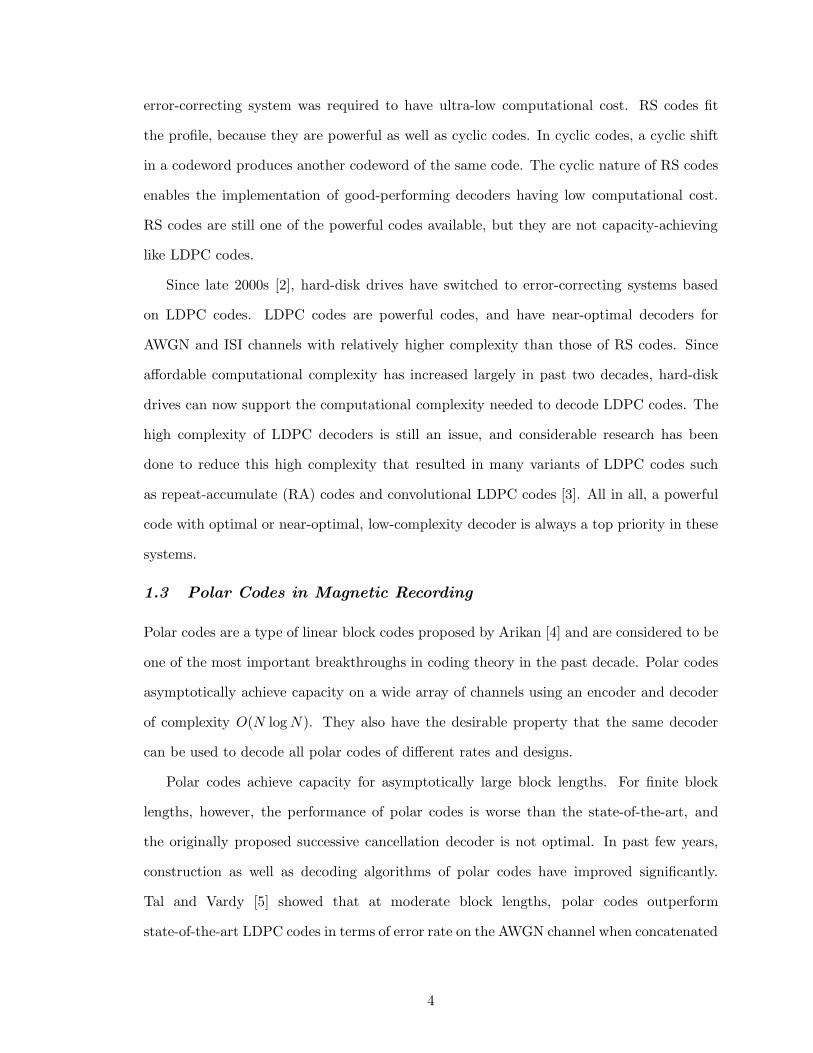
1.5 The majority of the area in the die micrograph of this LDPC decoder chip isoccupied by computational and memory units shown as SISO engine and Γ-,π-SRAM, respectively. Most of the rest of the area is occupied by the wiringnetwork connecting different parts of the chip shown as Ω-NETWORK. Theimage is taken from Mansour, M.M.; Shanbhag, N.R.,“A 640-Mb/s 2048-bitprogrammable LDPC decoder chip,” Solid-State Circuits, IEEE Journal of ,vol.41, no.3, pp.684,698, March 2006 ©2006 IEEE. . . . . . . . . . . . . . 8
1.6 A good decoder lies in the region close to the origin in three dimensionalspace of power, area and latency. This region directly corresponds to a regionclose to the origin in three dimensional space of computational complexity,memory requirement and latency. . . . . . . . . . . . . . . . . . . . . . . . 8
1.7 An ideal system consisting of polar codes and their soft-output decoder shouldlie in the highlighted region of the four-dimensional space. . . . . . . . . . 10
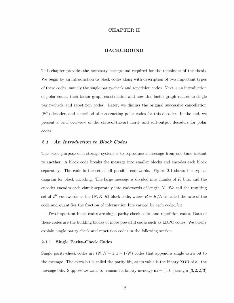
2.1 In a block code, the message is divided into blocks of K bits. Each block isthen independently encoded to a block of N coded bits using an encoder. . 13
2.2 The parity-check node takes all the input messages in the form of intrinsic
LLRs and produces the outbound message L(e)N−1. . . . . . . . . . . . . . . . 18
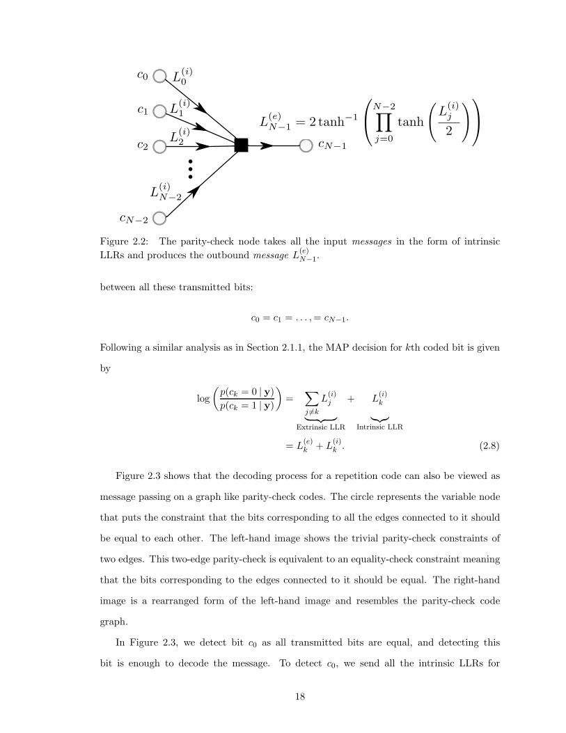
2.3 A (N, 1, 1/N) repetition code repeats the message bit N times giving rise toN − 1 trivial parity-check nodes with two edges as shown on the left. Theright-hand side image is the rearranged version of the left-hand side imagewith the equality-check node corresponding to c0 summing all incoming LLRsto produce an outgoing extrinsic LLR for c0. . . . . . . . . . . . . . . . . . 19
2.4 The encoder represents the relationship between encoded and uncoded bitsof a rate one-half polar code with I = 3, 5, 6, 7. The rectangles with ’+’sign represents binary XOR operation. . . . . . . . . . . . . . . . . . . . . . 22
ix

2.5 The basic structure in the encoder of polar code represents polar codesof length two. This basic encoder correspond to a parity-check and anequality-check constraint. . . . . . . . . . . . . . . . . . . . . . . . . . . . . 23
2.6 The factor graph represents the relationship between encoded and uncodedbits of a rate one-half polar code with I = 3, 5, 6, 7. . . . . . . . . . . . . 24
2.7 The trio (λ, φ, ω) can index all the nodes in the factor graph of polar codes. 25
2.8 The difference between the SC and the SCL decoder lies in the number ofpaths they keep while detecting any message bit. . . . . . . . . . . . . . . . 31
2.9 The BP decoder updates LLRs on a protograph-by-protograph basis. In asingle protograph, it updates four LLRs with two LLRs in both L and B. . 34
2.10 The polar code with BP decoding performs worse than the LDPC code withBP decoding on both the fronts: it requires a larger number of computationswhile requiring a larger Eb/N0 to achieve FER = 10−3 on a dicode channel. 35
2.11 The BP decoder for LDPC codes requires less than 50% of the memoryrequired by BP decoder for polar codes with N > 16. This relative memoryrequirement decreases monotonically and goes very low for practical blocklengths such as only 13% for a code of length 32768. . . . . . . . . . . . . . 36
3.1 System model for Lemma: 3.1 . . . . . . . . . . . . . . . . . . . . . . . . . . 38
3.2 At any depth λ ∈ 0, 1, . . . , n, Lλ(φ) for all φ ∈ 0, . . . , 2λ are stored inthe memory for Lλ(0), which is shown in green. . . . . . . . . . . . . . . . . 44
3.3 Memory elements required to store B with corresponding φ displayed nextto a particular Bλ(φ). In any iteration, the SCAN decoder does not needBλ(φ) : φ is even for the next iteration, and we can overwrite Bλ(0)(shown with green rectangles) at any depth λ with Bλ(φ) : φ is even, φ 6= 0(shown with yellow rectangles). On the other hand, the SCAN decoderrequires Bλ(φ) : φ is odd (shown with white rectangles) for processingin the next iteration, and therefore it will keep these memory locations asthey are. In this small example, we save five memory elements correspondingto B2(2),B3(2),B3(4) and B3(6). . . . . . . . . . . . . . . . . . . . . . . . 48
3.4 FER and BER performance of the SCAN decoder in the AWGN channel forN = 32768. We have optimized the polar code for Eb/N0 = 2.35 dB usingthe method of [1]. . . . . . . . . . . . . . . . . . . . . . . . . . . . . . . . . . 53
3.5 FER performance of the SCAN decoder in partial response channels for K =4096 and N = 8192. We have optimized the polar code for Eb/N0 = 1.4 dB(dicode) and Eb/N0 = 1.55 dB (EPR4) using the method of [1]. . . . . . . . 55
3.6 Memory efficiency improves with increasing block length. . . . . . . . . . . 56
x

4.1 Only P0, P1 and P2 are possible at depth n in the factor graph of the polarcodes. The inputs on the right of these three protographs specify whetherbit is free (in case of 0) or fixed (in case of ∞). In case of P0, P1 and P2,both of the output nodes have LLRs from the same set. For example for P0,the values in B0(0) corresponding to both the output nodes on the left haveLLRs from the set ∞, i.e., the LLRs in both of these nodes are stuck to∞.On the other hand in P6, LLRs corresponding to output nodes come from theset 0,∞, i.e., both the values are different unlike other three protographs. 62
4.2 The notation used in the proof of Theorem 4.2 is explained. . . . . . . . . . 65
4.3 An example design of a rate one-half polar code validates the properties. Onlyprotographs P0, P1 and P2 appear at depth λ = n (Special Prohibited PairsProperty). In the entire factor graph, P6, P7 and P8 do not occur (GeneralProhibited Pairs Property). All the node-groups have LLRs from either ofthe sets 0, ∞,R (Corollary 4.1). . . . . . . . . . . . . . . . . . . . . 70
4.4 Every type of protograph has an equivalent reduced form. . . . . . . . . . 71
4.5 The memory required for O is reduced by not storing the LLRs correspondingto rate-one and rate-zero subcodes. . . . . . . . . . . . . . . . . . . . . . . . 77
4.6 The normalized number of computations, memory requirement and latencyof the eSCAN decoder with LLR-skipping stays less than those of the SCANdecoder without LLR-skipping for a range of code rates. . . . . . . . . . . . 79
4.7 The polar code with eSCAN decoding has approximately the samecomplexity/power trade-off trend as the LDPC code with BP decoding.However, polar codes require approximately 0.4 dB higher Eb/N0 to achievethe same frame error rate on the dicode channel. . . . . . . . . . . . . . . . 80
5.1 The factor graph of a parent polar code of length N = 8 is a concatenationof two outer codes of length four with an inner code of length eight. . . . . 84
5.2 The computation of EXIT chart of the BCJR decoder/equalizer boils downto computing three LLRs: a priori LLRs LA, channel LLRs LC and extrinsicLLRs LE . . . . . . . . . . . . . . . . . . . . . . . . . . . . . . . . . . . . . . 86
5.3 The polar code of length N can be viewed as the concatenation of four outercodes C0, C1,C2 and C3 using an inner code. . . . . . . . . . . . . . . . . . . 87
5.4 The EXIT curve of polar codes follows a hill-like trajectory with two faces,two plateaus and one slope. . . . . . . . . . . . . . . . . . . . . . . . . . . . 89
5.5 The inner code serves as the parity check and repetition code of degree threewhen the decoder for C1 is unsuccessful and the decoder for C0 is successful,respectively. . . . . . . . . . . . . . . . . . . . . . . . . . . . . . . . . . . . . 91
5.6 When decoders for outer codes C0, C1, C2 and C3 are unsuccessful, the innercode acts like a mixture of degree-five parity-check codes. The extrinsicmutual information at the output of the multistage decoder is zero, becauseall the decoders for C0, C1, C2 and C3 are unable to decode the message. . . 92
xi

5.7 When the decoders for outer code C0 and C1 are successful and unsuccessful,respectively, the inner code becomes a code mixture of serially concatenateddegree-three parity-check and degree-three variable nodes. . . . . . . . . . . 92
5.8 The EXIT curve of polar codes follows a hill-like trajectory for four-level codes. 94
5.9 The EXIT curve of polar codes calculated from Section 5.3 approximatesthat obtained through Monte Carlo simulations. . . . . . . . . . . . . . . . 98
5.10 Polar codes constructed through the proposed method provide approximately0.6 dB and 0.9 dB gain in FER performance on EPR4 and E2PR4 channels,respectively, relative to the ones optimized for AWGN. . . . . . . . . . . . . 101
6.1 In turbo decoding, the decoder decodes the combination of two codes byexchanging soft information between two decoders. . . . . . . . . . . . . . . 106
xii

LIST OF SYMBOLS OR ABBREVIATIONS
APP A Posteriori Probability.
AWGN Additive White Gaussian Noise.
BCJR Bahl, Cocke, Jelinek and Raviv.
BEC Binary Erasure Channel.
BP Belief Propagation.
CRC Cyclic Redundancy Check.
DE Desntiy Evolution.
E2PR4 Extended-Extended Partial Response Class-4.
EPR4 Extended Partial Response Class-4.
EXIT Extrinsic Information Transfer.
HDD Hard-Disk Drive.
ISI Intersymbol Interference.
LDPC Low-Density Parity-Check.
LLR Log-Likelihood Ratio.
MAP Maximum a Posteriori Probability.
RA Repeat-Accumulate.
RS Reed-Solomon.
SC Successive Cancellation.
SCAN Soft Cancellation.
SCL Successive Cancellation List.
SNR Signal-to-Noise Ratio.
SSC Simplified Successive Cancellation.
xiii

SUMMARY
Powerful error-correcting codes have enabled a dramatic increase in the bit density
on the recording medium of hard-disk drives (HDDs). Error-correcting codes in magnetic
recording require a low-complexity decoder and a code design that delivers a target
error-rate performance. This dissertation proposes an error-correcting system based on
polar codes incorporating a fast, low-complexity, soft-output decoder and a design that is
optimized for error-rate performance in the magnetic recording channel.
LDPC codes are the state-of-the-art in HDDs, providing the required error-rate
performance on high densities at the cost of increased computational complexity of the
decoder. Substantial research in LDPC codes has focused on reducing decoder complexity
and has resulted in many variants such as quasi-cyclic and convolutional LDPC codes.
Polar codes are a recent and important breakthrough in coding theory, as they achieve
capacity on a wide spectrum of channels using a low-complexity successive cancellation
decoder. Polar codes make a strong case for magnetic recording, because they have low
complexity decoders and adequate finite-length error-rate performance. In their current
form, polar codes are not feasible for magnetic recording for two reasons. Firstly, there is no
low-complexity soft-output decoder available for polar codes that is required for turbo-based
equalization of the magnetic recording channel. The only soft-output decoder available to
date is a message passing based belief propagation decoder that has very high computational
complexity and is not suitable for practical implementations. Secondly, current polar codes
are optimized for the AWGN channel only, and may not perform well under turbo-based
detector for ISI channels.
This thesis delivers a powerful low-complexity error-correcting system based on polar
codes for ISI channels. Specifically, we propose a low-complexity soft-output decoder for
polar codes that achieves better error-rate performance than the belief propagation decoder
for polar codes while drastically reducing the complexity. We further propose a technique
xiv
for polar code design over ISI channels that outperforms codes for the AWGN channel in
terms of error rate under the proposed soft-output decoder.
Altogether, this thesis takes polar codes from the point of being infeasible for magnetic
recording application and puts them at a competitive position with the state-of-the-art.
xv
CHAPTER I
INTRODUCTION
Storage devices such as DVDs, hard-disks and flash drives are the backbone of modern
data-driven life. Each of these devices is suitable for a specific application. DVDs suit
applications where data is only read and is not written or erased such as software and
movie distribution. Flash drives suit applications that require little storage with high read
and write speed such as temporary personal data storage. Magnetic recording devices such
as hard-disk drives cater for the bulk of today’s data storage needs. Magnetic recording
devices are popular, because they offer a non-volatile, high-speed, low-cost and physically
manageable solution for data storage. For these reasons, the hard disk is an integral part
of almost every computer system and data center.
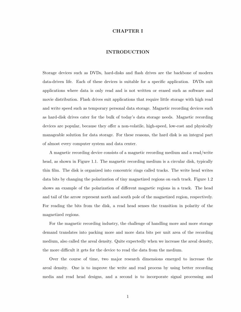
A magnetic recording device consists of a magnetic recording medium and a read/write
head, as shown in Figure 1.1. The magnetic recording medium is a circular disk, typically
thin film. The disk is organized into concentric rings called tracks. The write head writes
data bits by changing the polarization of tiny magnetized regions on each track. Figure 1.2
shows an example of the polarization of different magnetic regions in a track. The head
and tail of the arrow represent north and south pole of the magnetized region, respectively.
For reading the bits from the disk, a read head senses the transition in polarity of the
magnetized regions.
For the magnetic recording industry, the challenge of handling more and more storage
demand translates into packing more and more data bits per unit area of the recording
medium, also called the areal density. Quite expectedly when we increase the areal density,
the more difficult it gets for the device to read the data from the medium.
Over the course of time, two major research dimensions emerged to increase the
areal density. One is to improve the write and read process by using better recording
media and read head designs, and a second is to incorporate signal processing and
1

Read/Write Head
Tracks
Magnetic Recording
Medium
Figure 1.1: A magnetic recording device consists of a magnetic recording medium and aread/write head. The write head writes data bits on the magnetic recording medium inconcentric rings called tracks.
Write Head
N S
Figure 1.2: The write head writes data bits on a track by changing the polarity of smallmagnetized regions.
error-correcting techniques to make the read process robust against errors. This thesis
extends research in the dimension of error-correcting techniques and proposes a new,
competitive error-correcting system based on polar codes.
1.1 Magnetic Recording Channel as a Communication Channel
In error-control coding, a transmitter wishing to send a K-bit message will first encode it
into a sequence of N > K coded bits called the codeword before sending through a noisy
channel. The set of all possible codewords is called the code. At the receiver, the decoder
maps the noisy version of the transmitted codeword to a K-bit decision message. N −K
additional bits make the communication system more reliable. The price for this extra
reliability is the reduction in useful data rate or storage capacity for the HDD, by a factor
of 1−K/N .
A magnetic recording system is like a communication system. The read/write process
2

ENCODER DECODER
Channel
ENCODER DECODER
Recording Medium
Figure 1.3: Hard-disk write/read process is similar to transmitting on a traditionalcommunication channel except that instead of transmitting from one physical location tothe other, hard-disk drives transmit data from one time instant (when the user writes thedata) to the other (when the user reads the data). An example of mapping between messageand coded bits is also shown below the encoder. In this example, the transmitter sends themessage bit twice and for this repetition, the code is called the repetition code.
is similar to a communication system with the write process acting as the transmitter, the
read process acting as the receiver, and the recording medium acting as the channel. Unlike
communication systems, in which we transmit the data from one physical location to the
other, the recording devices transmit data from one time instant to the other. Figure 1.3
compares the basic components of a communication system with those of a recording system.
The effectiveness of an error-correcting system broadly depends on both the encoder
and the decoder. Often the code must be designed to match the specific characteristics of
the channel being considered. For example, a code designed for the AWGN channel may
not perform well on ISI channels. Secondly, the decoder should be optimal or near-optimal
in error-rate performance for a specific channel and should also admit a memory-efficient,
low-complexity, low-latency hardware implementation.
1.2 History of Error-Correcting Codes in Magnetic Recording
In 1990s, hard-disk drives employed Reed-Solomon (RS) codes for their error-correcting
systems. At that time, the affordable computational power was very low, and the
3
error-correcting system was required to have ultra-low computational cost. RS codes fit
the profile, because they are powerful as well as cyclic codes. In cyclic codes, a cyclic shift
in a codeword produces another codeword of the same code. The cyclic nature of RS codes
enables the implementation of good-performing decoders having low computational cost.
RS codes are still one of the powerful codes available, but they are not capacity-achieving
like LDPC codes.
Since late 2000s [2], hard-disk drives have switched to error-correcting systems based
on LDPC codes. LDPC codes are powerful codes, and have near-optimal decoders for
AWGN and ISI channels with relatively higher complexity than those of RS codes. Since
affordable computational complexity has increased largely in past two decades, hard-disk
drives can now support the computational complexity needed to decode LDPC codes. The
high complexity of LDPC decoders is still an issue, and considerable research has been
done to reduce this high complexity that resulted in many variants of LDPC codes such
as repeat-accumulate (RA) codes and convolutional LDPC codes [3]. All in all, a powerful
code with optimal or near-optimal, low-complexity decoder is always a top priority in these
systems.
1.3 Polar Codes in Magnetic Recording
Polar codes are a type of linear block codes proposed by Arikan [4] and are considered to be
one of the most important breakthroughs in coding theory in the past decade. Polar codes
asymptotically achieve capacity on a wide array of channels using an encoder and decoder
of complexity O(N logN). They also have the desirable property that the same decoder
can be used to decode all polar codes of different rates and designs.
Polar codes achieve capacity for asymptotically large block lengths. For finite block
lengths, however, the performance of polar codes is worse than the state-of-the-art, and
the originally proposed successive cancellation decoder is not optimal. In past few years,
construction as well as decoding algorithms of polar codes have improved significantly.
Tal and Vardy [5] showed that at moderate block lengths, polar codes outperform
state-of-the-art LDPC codes in terms of error rate on the AWGN channel when concatenated
4

Serial Concatenation
+ENCODER ISISOFT-OUTPUT
DETECTORDECODER
Soft Information
AWGN
Turbo Equalizer
Figure 1.4: In turbo equalization, the receiver iteratively exchanges the soft informationbetween the soft-output detector and the decoder for error-correcting code.
even with the simplest cyclic redundancy check (CRC) codes using a successive-cancellation
list decoder [5]. The work of Tal and Vardy produced a powerful code with near-optimal
performance and a relatively low-complexity decoder, but these results were limited to the
AWGN channel only.
The magnetic recording channel is an intersymbol interference ISI channel. One famous
detection strategy for intersymbol interference channels is turbo equalization [6], in which a
detector for the ISI channel and the decoder for error-correcting code iteratively exchange
reliability information known as soft information about the coded bits. A common way of
representing soft information for binary symbols is the log-likelihood ratio (LLR), which is
defined as
LLR = log
(Likelihood of a bit being zero
Likelihood of a bit being one
)
.
The sign of the LLR describes the decision whether the bit is zero or one, whereas its
magnitude corresponds to the reliability of this decision. The higher the magnitude is, the
more confident the decoder is about its decision. For instance, if the LLR is positive, it
means the decoder is more confident about the bit being zero than its being one. In the
extreme case when this LLR is +∞, the decoder is absolutely sure that the bit is zero. If
the decoder decides only with absolute belief delivering only +∞ and −∞ LLRs, it is called
a hard-output decoder. The iterative exchange of this soft information gradually reduces
the error rate resulting in the improved reliability of a turbo-based communication system.
Figure 1.4 shows the basic system diagram for a turbo-based equalizer.
For turbo-based receivers, polar codes need a soft-output decoder that can produce
the reliability information to be exchanged. Additionally, polar codes are expected to
5

perform well in turbo-based receivers if codes are optimized for error-rate performance in
ISI channels. Therefore, the goal of the thesis can be broadly defined as follows: to construct
a turbo-based system for polar codes with error-rate performance close to state-of-the-art
LDPC-based systems. We precisely describe this goal in the next section.
1.4 Thesis Goal: A Tale of Four Metrics
In the previous section, we established that the desirable properties of polar codes make
them an excellent candidate for magnetic recording system, but to enable polar codes
in this application, we need a soft-output decoder to decode these codes under turbo
equalization framework. Furthermore, code designs matched to the characteristics of ISI
channels often outperform the codes designed for the AWGN channel. Therefore, we expect
better error-rate performance with the optimized code designs compared to the designs for
the AWGN channel. This section further discusses these requirements.
1.4.1 Requirements from a Decoder
The requirements for a soft-output decoder stem from the fact that eventually it is realized
on a hardware platform. The hardware has three important specifications, namely the power
consumption, area utilization and the number of bits it can process per second, also called
throughput. The following aspects of a decoder directly affect these three specifications:
1. Computational Complexity: Computational complexity relates to the number of
computations (such as additions, multiplications and copy operations) required by
a decoder. In general, higher computational complexity results in increased power
consumption, higher area utilization and slower speed of operation of the device
[7]. Therefore, an efficient decoder should minimize the number of operations while
delivering a certain quality of service in terms of error rate.
2. Memory Requirement: A decoder requires not only computational hardware but
also memory to store interval variables such as intermediate states. In general, a
larger memory requirement translates to higher power and area utilization [7] on the
hardware platform. Therefore, an efficient decoder should minimize the amount of
6

memory it uses as much as possible.
3. Latency or Throughput: Latency is usually defined in a normalized fashion as the
number of clock cycles required to process one bit, and is inversely related to the
throughput of the decoder [8]. A decoder with higher latency requires a higher clock
than one with lower latency to achieve the same throughput. For example, consider
two decoders A and B of normalized latency of 10 and 20 cycles per bit, respectively.
To achieve a throughput of 1Mbps, the decoder A and B need a clock of 10 and 20 MHz,
respectively. In general, the higher clock rate results in higher power consumption of
hardware, and as decoder B requires a higher clock, it consumes more power than
decoder A. Therefore, a decoder should minimize its latency as much as possible.
In short, power consumption, area utilization and latency are three key performance
metrics for hardware implementation of any decoder. The two major contributors to power
and area consumption are computational logic and memory. To elaborate this point further,
Figure 1.5 shows the die micrograph of the LDPC decoder chip taken from [9]. The die
shows that the majority of the area is taken up by the SISO engine corresponding to the
computational unit and memory shown as Γ-SRAM and π-SRAM. The interconnect network
connecting different parts of the chip shown as Ω-NETWORK, occupies most of the rest of
the area.
Figure 1.6 summarizes this section and shows that a practically feasible decoder lies
as close to the origin in three dimensional space of power, area and latency. This
position directly corresponds to a region close to the origin in three dimensional space
of computational complexity, memory required and the same latency.
1.4.2 Requirements from a Code/Encoder
Even if we have near-optimal performance by a decoder, the complete system may not deliver
in terms of error rates if the underlying code itself is weak. Therefore, the requirement from
the code is very straight forward – it should produce a lower error rate in a channel when
decoded by a specific decoder. For example, early LDPC codes were not powerful enough
to deliver better error rates on the AWGN channel, even though their decoder provided
7
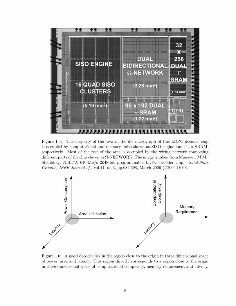
Figure 1.5: The majority of the area in the die micrograph of this LDPC decoder chipis occupied by computational and memory units shown as SISO engine and Γ-, π-SRAM,respectively. Most of the rest of the area is occupied by the wiring network connectingdifferent parts of the chip shown as Ω-NETWORK. The image is taken from Mansour, M.M.;Shanbhag, N.R.,“A 640-Mb/s 2048-bit programmable LDPC decoder chip,” Solid-StateCircuits, IEEE Journal of , vol.41, no.3, pp.684,698, March 2006 ©2006 IEEE.
Pow
er
Co
nsu
mptio
n
Area Utilization
Late
ncy
Co
mpu
tation
al
Co
mple
xity
Memory
Requirement
Late
ncy
Figure 1.6: A good decoder lies in the region close to the origin in three dimensional spaceof power, area and latency. This region directly corresponds to a region close to the originin three dimensional space of computational complexity, memory requirement and latency.
8

near-optimal performance. Later Richardson, Shokrollahi and Urbanke designed better
LDPC codes that outperformed the state-of-the-art codes at that time for the AWGN
channel [10]. In short, a code should be optimized for any required channel to deliver
desired error rates using an optimal or near-optimal decoder.
1.4.3 Summary
Figure 1.7 summarizes all the requirements for a magnetic recording error-control system.
In a four-dimensional space of these requirements, the ideal system (a code and its decoder)
should lie as close to the origin in the highlighted region as possible, and this thesis primarily
focuses on coming up with such a system for polar codes. In other words, this thesis
produces both the optimized polar codes for ISI channels as well as a low-complexity,
soft-output decoder for their decoding under the turbo framework, and delivers a powerful
error-correcting system for magnetic recording application.
Figure 1.7 also describes the structure of the thesis. The thesis is structured as follows:
1. In Chapter 2, we provide a brief introduction to different concepts needed to explain
rest of the thesis. We start with an introduction to block codes and then provide
a tutorial on two examples block codes, namely parity-check codes and repetition
codes. We then introduce polar codes with their factor graph description and show
how parity-check and repetition codes combine to form polar codes. In the end, we
discuss various soft-output and hard-output decoding algorithms.
2. In Chapter 3, we propose a low-complexity soft-output decoder called the soft
cancellation (SCAN) decoder. The SCAN decoder is based on the SCAN schedule for
message updates in the message passing decoder of polar codes. The SCAN schedule,
in contrast with the original flooding schedule, drastically reduces the computational
complexity of the message passing decoder. The reason for the substantial complexity
reduction is better dissemination of information in the factor graph with the SCAN
schedule compared to the flooding schedule. The SCAN schedule results in rapid
convergence of message passing algorithm while providing soft outputs needed for
turbo processing. Additionally, we propose a technique to reduce the memory
9

CO
MP
UT
AT
ION
AL
CO
MP
LE
XIT
YMEMORY REQUIRED
LATENCY
ERROR R
ATE
Figure 1.7: An ideal system consisting of polar codes and their soft-output decoder shouldlie in the highlighted region of the four-dimensional space.
requirement of the SCAN decoder based on the idea that the decoder can overwrite
soft information corresponding to some of the nodes in the factor graph. We identify
the nodes for which we can overwrite the soft information and reuse the memory to
reduce the memory requirement of the decoder. We also provide error-rate curves for
AWGN and ISI channels to show that the SCAN decoder outperforms the BP decoder
for polar codes and performs close to the BP decoder of LDPC codes.
3. In Chapter 4, we have two major contributions. Firstly, we extend the simplified
successive-cancellation (SSC) principle of Alamdar-Yazdi and Kschischang [11] to the
SCAN decoder and reduce its latency and computational complexity. Secondly, we
prove that the construction of polar codes exhibit two properties called the special
10
prohibited pair property and the general prohibited pair property. We apply these
properties to the implementation of the SCAN decoder that reduces the memory
requirement of the decoder even further. We call the resulting SCAN decoder with
the improvements in latency, computational complexity and memory requirement the
enhanced SCAN (eSCAN) decoder. The eSCAN has the same error-rate performance
as the SCAN decoder but with reduced latency, computational complexity and
memory requirement.
4. In Chapter 5, we propose a method to design polar codes for ISI channels. The
method is based on the idea that the EXIT chart of an optimal code matches that
of an ISI channel under iterative decoding. We show that in a multilevel description
of polar codes, we can change the rates of polar codes in different levels in order to
match the EXIT chart to that of an ISI channel. We demonstrate using simulations
that polar codes designed using this method outperform the ones designed for the
AWGN channel when decoded using the SCAN decoder, and perform close to the
state-of-the-art LDPC codes with the belief propagation decoder.
5. In Chapter 6, we conclude the thesis by summarizing our contributions and outlining
a few directions in which our work can be extended.
11
CHAPTER II
BACKGROUND
This chapter provides the necessary background required for the remainder of the thesis.
We begin by an introduction to block codes along with description of two important types
of these codes, namely the single parity-check and repetition codes. Next is an introduction
of polar codes, their factor graph construction and how this factor graph relates to single
parity-check and repetition codes. Later, we discuss the original successive cancellation
(SC) decoder, and a method of constructing polar codes for this decoder. In the end, we
present a brief overview of the state-of-the-art hard- and soft-output decoders for polar
codes.
2.1 An Introduction to Block Codes
The basic purpose of a storage system is to reproduce a message from one time instant
to another. A block code breaks the message into smaller blocks and encodes each block
separately. The code is the set of all possible codewords. Figure 2.1 shows the typical
diagram for block encoding. The large message is divided into chunks of K bits, and the
encoder encodes each chunk separately into codewords of length N . We call the resulting
set of 2K codewords as the (N,K,R) block code, where R = K/N is called the rate of the
code and quantifies the fraction of information bits carried by each coded bit.
Two important block codes are single parity-check codes and repetition codes. Both of
these codes are the building blocks of more powerful codes such as LDPC codes. We briefly
explain single parity-check and repetition codes in the following section.
2.1.1 Single Parity-Check Codes
Single parity-check codes are (N,N − 1, 1 − 1/N) codes that append a single extra bit to
the message. The extra bit is called the parity bit, as its value is the binary XOR of all the
message bits. Suppose we want to transmit a binary message m = [ 1 0 ] using a (3, 2, 2/3)
12
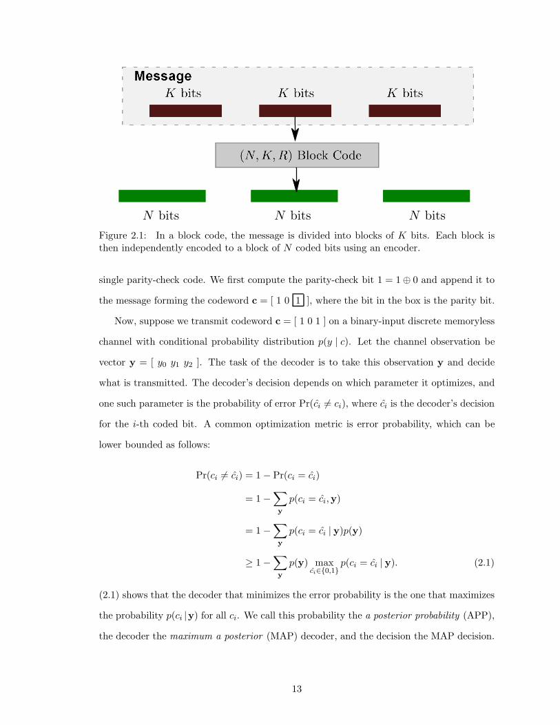
Figure 2.1: In a block code, the message is divided into blocks of K bits. Each block isthen independently encoded to a block of N coded bits using an encoder.
single parity-check code. We first compute the parity-check bit 1 = 1⊕ 0 and append it to
the message forming the codeword c = [ 1 0 1 ], where the bit in the box is the parity bit.
Now, suppose we transmit codeword c = [ 1 0 1 ] on a binary-input discrete memoryless
channel with conditional probability distribution p(y | c). Let the channel observation be
vector y = [ y0 y1 y2 ]. The task of the decoder is to take this observation y and decide
what is transmitted. The decoder’s decision depends on which parameter it optimizes, and
one such parameter is the probability of error Pr(ci 6= ci), where ci is the decoder’s decision
for the i-th coded bit. A common optimization metric is error probability, which can be
lower bounded as follows:
Pr(ci 6= ci) = 1− Pr(ci = ci)
= 1−∑
y
p(ci = ci,y)
= 1−∑
y
p(ci = ci | y)p(y)
≥ 1−∑
y
p(y) maxci∈0,1
p(ci = ci | y). (2.1)
(2.1) shows that the decoder that minimizes the error probability is the one that maximizes
the probability p(ci |y) for all ci. We call this probability the a posterior probability (APP),
the decoder the maximum a posterior (MAP) decoder, and the decision the MAP decision.
13

The MAP decision ci is given by
ci(y) = argmaxci
p(ci | y)
= argmaxci
p(y | ci)p(ci)p(y)
(Bayes’ Rule)
= argmaxci
p(y | ci)p(ci), (2.2)
where in the last step, we omitted p(y), as it does not depend on ci and does not take part
in the optimization process.
Suppose we are interested in detecting bit c2. We calculate the MAP decision for c2
by first computing the objective function in (2.2) for both the values c2 ∈ 0, 1 and then
finding the value of ci that maximizes it. We start by computing p(y | ci = 0)Pr(ci = 0) as
follows:
p(y | c2 = 0)Pr(c2 = 0) = p(y0, y1 | c2 = 0)︸ ︷︷ ︸
from y0, y1
p(y2 | c2 = 0)︸ ︷︷ ︸
from y2
Pr(c2 = 0).︸ ︷︷ ︸
Message Source
(2.3)
The right-hand side of (2.3) depends on the following:
1. p(y0, y1 | c2 = 0): This is likelihood of c2 being zero given noisy observations y0 and
y1 of c0 and c1, respectively. This term carries the information that y0 and y1 convey
about c2.
2. p(y2 | c2 = 0): This is likelihood of c2 being zero given noisy observation y2. This term
carries the information that y2 conveys about c2.
3. Pr(c2 = 0): Assuming m0 and m1 are equally likely to be zero or one, c2 is equally
likely to be zero or one as well and Pr(c2 = 0) = 1/2.
14

Expanding p(y0, y1 | c2 = 0) term on the right-hand side of (2.3), we get
p(y0, y1 | c2 = 0) =∑
c0,c1
p(y0, y1, c0, c1 | c2 = 0)
=∑
c0,c1
p(y0, y1 | c0, c1, c2 = 0)p(c0, c1 | c2 = 0)
= p(y0, y1 | c0 = 0, c1 = 0, c2 = 0)Pr(c0 = 0, c1 = 0 | c2 = 0)
+ p(y0, y1 | c0 = 1, c1 = 0, c2 = 0)Pr(c0 = 1, c1 = 0 | c2 = 0)
+ p(y0, y1 | c0 = 0, c1 = 1, c2 = 0)Pr(c0 = 0, c1 = 1 | c2 = 0)
+ p(y0, y1 | c0 = 1, c1 = 1, c2 = 0)Pr(c0 = 1, c1 = 1 | c2 = 0). (2.4)
Since c0 and c1 must be identical when c2 = 0, the middle two terms are zero, and (2.4)
simplifies to:
p(y0, y1 | c2 = 0) = p(y0, y1 | c0 = 0, c1 = 0, c2 = 0)Pr(c0 = 0, c1 = 0 | c2 = 0)
+ p(y0, y1 | c0 = 1, c1 = 1, c2 = 0)Pr(c0 = 1, c1 = 1 | c2 = 0). (2.5)
But since the message source is independently and uniformly distributed, we have
Pr(c0 = 1, c1 = 1 | c2 = 0) = Pr(m0 = 1,m1 = 1 | c2 = 0) =1
2.
Therefore, p(y0, y1 | c2 = 0) in (2.5) is simplified to
p(y0, y1 | c2 = 0) =1
2
(
p(y0, y1 | c0 = 0, c1 = 0, c2 = 0) + p(y0, y1 | c0 = 1, c1 = 1, c2 = 0)
)
=1
2
(
p(y0 | c0 = 0)p(y1 | c1 = 0) + p(y0 | c0 = 1)p(y1 | c1 = 1)
)
.
Using this value of p(y0, y1 | c2 = 0) in (2.3), we get
p(y |c2 =0)Pr(c2 =0)=1
4
(
p(y0 |c0 =0)p(y1 |c1 =0)+p(y0 |c0 =1)p(y1 |c1 =1)
)
p(y2 |c2 =0),
where once again we have used the fact that the source is uniformly distributed, and Pr(c2 =
0) = 1/2. By following the same procedure we used for p(y | c2 = 0)Pr(c2 = 0), we compute
p(y |c2 =1)Pr(c2 =1)=1
4
(
p(y0 |c0 =0)p(y1 |c1 =1)+p(y0 |c0 =1)p(y1 |c1 =0)
)
p(y2 |c2 =1).
15

The last step of the decoder is to use these two probabilities to make a decision about
i-th bit, according to
p(ci = 0 | y)0≷1p(ci = 1 | y)
or
p(y | ci = 0)Pr(ci = 0)0≷1p(y | ci = 1)Pr(ci = 1).
In simple words, it means that decide the bit is zero if
p(y | ci = 0)Pr(ci = 0) > p(y | ci = 1)Pr(ci = 1)
and one otherwise. We can further simplify it by converting it into a ratio and taking
natural logarithm of both sides as follows:
p(y | ci = 0)Pr(ci = 0)
p(y | ci = 1)Pr(ci = 1)
0≷11
log
(p(y | ci = 0)Pr(ci = 0)
p(y | ci = 1)Pr(ci = 1)
)0≷10. (2.6)
The left-hand side of (2.6) can further be simplified as
log
(p(y | ci = 0)Pr(ci = 0)
p(y | ci = 1)Pr(ci = 1)
)
= log
(p(y0 | c0 = 0)p(y1 | c1 = 0) + p(y0 | c0 = 1)p(y1 | c1 = 1)
p(y0 | c0 = 0)p(y1 | c1 = 1) + p(y0 | c0 = 1)p(y1 | c1 = 0)
× p(y2 | c2 = 0)
p(y2 | c2 = 1)
)
= log
p(y0 | c0=0)p(y0 | c0=1)
p(y1 | c1=0)p(y1 | c1=1) + 1
p(y0 | c0=0)p(y0 | c0=1) +
p(y1 | c1=0)p(y1 | c1=1)
× p(y2 | c2 = 0)
p(y2 | c2 = 1)
= log
((ℓ0ℓ1 + 1)ℓ2ℓ0 + ℓ1
)
, (2.7)
where
ℓj =p(yj | cj = 0)
p(yi | ci = 1).
We can use trigonometric identities to reduce (2.7) to
log
(p(c2 = 0 | y)p(c2 = 1 | y)
)
= 2 tanh−1
(
tanh
(
L(i)0
2
)
tanh
(
L(i)1
2
))
︸ ︷︷ ︸
Extrinsic LLR
+ L(i)2
︸︷︷︸
Intrinsic LLR
= L(e)2 + L
(i)2
16

where
L(i)j = log
(p(yj | cj = 0)
p(yj | cj = 1)
)
.
Extrinsic LLRs provide the reliability information generated from code constraints, whereas
intrinsic LLRs provide the reliability information directly gleaned from channel observations.
To make a decision about bit c2, the decoder adds these two LLRs to compute the so-called
full LLR and declares the bit zero if the sum is positive and one otherwise, as described by
the rule (2.6).
We can follow a similar analysis for two other bits c0 and c1 to get the expression for
their full LLRs. In general, for a (N,N − 1, 1− 1/N) code the extrinsic LLR and full LLR
of kth bit are given by
L(e)k = 2 tanh−1
∏
j 6=k
tanh
(
L(i)j
2
)
,
and
L(full)k = L
(e)k + L
(i)k ,
respectively.
Figure 2.2 shows that the whole decision process as message passing along the edges
on a graph. The rectangle represents a parity-check node, whereas the circles represent
variable nodes. The parity-check node represents the constraint that all its inputs should
sum to zero. The figure shows that to compute the extrinsic LLR for the parity bit, we send
intrinsic LLRs observed from the channel on the edges corresponding to variable nodes c0
to cN−2. The parity-check node takes all these messages from different variable nodes and
computes the outbound message L(e)N−1. The same process can be repeated for all other bits
to compute their extrinsic LLRs and eventually their full LLRs for detection.
2.1.2 Repetition Codes
An (N, 1, 1/N) repetition code repeats every message bit N times so that each message bit
m0 gets mapped to the codeword c = [m0,m1, . . . ,mN−1].
Suppose we want to transmit a zero bit using a (N, 1, 1/N) repetition code. This code
takes the message bit and transmits it N times producing the following equality constraint
17
...
Figure 2.2: The parity-check node takes all the input messages in the form of intrinsic
LLRs and produces the outbound message L(e)N−1.
between all these transmitted bits:
c0 = c1 = . . . ,= cN−1.
Following a similar analysis as in Section 2.1.1, the MAP decision for kth coded bit is given
by
log
(p(ck = 0 | y)p(ck = 1 | y)
)
=∑
j 6=k
L(i)j
︸ ︷︷ ︸
Extrinsic LLR
+ L(i)k
︸︷︷︸
Intrinsic LLR
= L(e)k + L
(i)k . (2.8)
Figure 2.3 shows that the decoding process for a repetition code can also be viewed as
message passing on a graph like parity-check codes. The circle represents the variable node
that puts the constraint that the bits corresponding to all the edges connected to it should
be equal to each other. The left-hand image shows the trivial parity-check constraints of
two edges. This two-edge parity-check is equivalent to an equality-check constraint meaning
that the bits corresponding to the edges connected to it should be equal. The right-hand
image is a rearranged form of the left-hand image and resembles the parity-check code
graph.
In Figure 2.3, we detect bit c0 as all transmitted bits are equal, and detecting this
bit is enough to decode the message. To detect c0, we send all the intrinsic LLRs for
18

...
...
Figure 2.3: A (N, 1, 1/N) repetition code repeats the message bit N times giving rise toN − 1 trivial parity-check nodes with two edges as shown on the left. The right-hand sideimage is the rearranged version of the left-hand side image with the equality-check nodecorresponding to c0 summing all incoming LLRs to produce an outgoing extrinsic LLR forc0.
c1, c2, . . . , cN−1 to the variable node of c0. The variable node sums all the incoming messages
and produce the extrinsic LLR L(e)0 that we add to intrinsic LLR L
(i)0 calculating the full
LLR. The sign of this full LLR decides about the message bit. It is easy to see that the full
LLR for all the bits is equal to∑N−1
j=0 L(i)j , highlighting once again that no matter which bit
we decode, the resulting decision for the message bit stays the same. However, note that
extrinsic LLRs corresponding to different bits will generally be different.
2.2 An Introduction to Polar Codes
In the previous section, we discussed block codes and their two important examples. This
section builds on this discussion and introduces polar codes that are complex combination
of the basic parity-check and repetition codes.
2.2.1 Generator Matrix and Encoding
Like all other linear binary block codes, polar codes encode a block of K bits to a block of
N bits using a generator matrix G. The difference is in the construction of this generator
matrix.
Consider a (N,K,R) polar code of length N , dimension K and rate R = K/N . The
generator matrix G for this polar code can be constructed in four steps:
19

1. Construct FN using FN = F⊗n2 , where n = log2(N), (.)⊗ denotes the nth Kronecker
power and
F2 :=
1 0
1 1
.
2. Construct GN using GN = BFN , where B is called the bit-reversal matrix. B is a
permutation matrix ensuring that
x = yB =⇒ xbn−1,bn−2,...,b0 = yb0,b1,...,bn−1,
where b1, . . . , bn ∈ 0, 1 represent the binary expansion of the index of an element in
row vectors x and y [4]. For example, x1 = x0,0,1 for n = 3. The significance of this
permutation operation will be explained in Section 2.2.2.
3. Remove N − K rows with indices from the set I c ⊂ 0, 1, . . . , N − 1 from GN to
obtain a K ×N matrix G. The codeword v is given by
v = mG.
4. An alternative to the last step is to take the message vector m = [m0 m1, . . . , m(K−1)]
of length K and form another vector u = [u0 u1 , . . . , u(N−1)] such that m appears
in u on the index set I ⊆ 0, 1, 2, . . . , N − 1 and zero bit appears on I c. In this
case, v = uGN.
In literature, the set I is usually referred to as the set of ’free indices’ and the complement
I c as the set of ’frozen indices’. The construction of polar codes is equivalent to constructing
I and is discussed in Section 2.3.
Example 2.1. Suppose we want to generate a (8, 4, 0.5) polar code with frozen indices
20
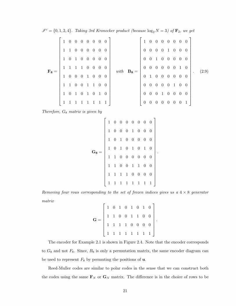
I c = 0, 1, 2, 4. Taking 3rd Kronecker product (because log2N = 3) of F2, we get
F8 =
1 0 0 0 0 0 0 0
1 1 0 0 0 0 0 0
1 0 1 0 0 0 0 0
1 1 1 1 0 0 0 0
1 0 0 0 1 0 0 0
1 1 0 0 1 1 0 0
1 0 1 0 1 0 1 0
1 1 1 1 1 1 1 1
with B8 =
1 0 0 0 0 0 0 0
0 0 0 0 1 0 0 0
0 0 1 0 0 0 0 0
0 0 0 0 0 0 1 0
0 1 0 0 0 0 0 0
0 0 0 0 0 1 0 0
0 0 0 1 0 0 0 0
0 0 0 0 0 0 0 1
. (2.9)
Therefore, G8 matrix is given by
G8 =
1 0 0 0 0 0 0 0
1 0 0 0 1 0 0 0
1 0 1 0 0 0 0 0
1 0 1 0 1 0 1 0
1 1 0 0 0 0 0 0
1 1 0 0 1 1 0 0
1 1 1 1 0 0 0 0
1 1 1 1 1 1 1 1
.
Removing four rows corresponding to the set of frozen indices gives us a 4 × 8 generator
matrix
G =
1 0 1 0 1 0 1 0
1 1 0 0 1 1 0 0
1 1 1 1 0 0 0 0
1 1 1 1 1 1 1 1
.
The encoder for Example 2.1 is shown in Figure 2.4. Note that the encoder corresponds
to G8 and not F8. Since, B8 is only a permutation matrix, the same encoder diagram can
be used to represent F8 by permuting the positions of u.
Reed-Muller codes are similar to polar codes in the sense that we can construct both
the codes using the same FN or GN matrix. The difference is in the choice of rows to be
21

UN
CO
DE
D B
ITS
EN
CO
DE
D B
ITS
+
+
+
+
+
+
+
+
+
+
+
+
Figure 2.4: The encoder represents the relationship between encoded and uncoded bits ofa rate one-half polar code with I = 3, 5, 6, 7. The rectangles with ’+’ sign representsbinary XOR operation.
removed. We can construct a (r,m) Reed-Muller code by keeping all the rows in FN with
Hamming weight greater than or equal to 2m−r [12]. In other words, in Reed-Muller codes
the rows with low Hamming weights are removed. In polar codes, a channel-specific rule
determines the rows to be removed and will be discussed in Section 2.3.
The polar code in Example 2.1 with generator matrix G is also a (1, 3) Reed-Muller
code [12]. Note that G is obtained by removing all the rows with Hamming weight less
than 23−1 = 4 in G8. Example 2.1 is a special case in which the choice of the rows to be
removed happens to be the same for Reed-Muller and polar codes, and in general, both
codes will be different.
2.2.2 The Factor Graph Representation of Polar Codes
Factor graphs are a graphical way of representing relationship between two set of variables
[13]. This graphical representation is specially beneficial when the relationship to be
represented can be factored into relationships between subsets of these variables. The
factor graph for polar codes can be understood with the help of parity-check and repetition
codes discussed in Section 2.1.
Figure 2.5 shows the basic structure in the encoder of polar codes that is also the
22

+
Figure 2.5: The basic structure in the encoder of polar code represents polar codes of lengthtwo. This basic encoder correspond to a parity-check and an equality-check constraint.
encoder of a length-two polar code. Two bits u0 and u1 add to produce the first codeword
bit c0, whereas the second codeword bit c1 is simply u1. As discussed in Section 2.1.1,
we can decode u0 using the parity-check node, whereas a variable node can represent the
equality constraint of c1 and u1 as discussed in Section 2.1.2. Therefore, we can convert
the constraints between message bits and codeword bits using a parity-check and variable
node, as shown in Figure 2.5.
Note that the bottom parity-check node is essentially an equality check node and can be
removed as well. The reason for this additional parity-check node is to make the decoder’s
graph a bipartite one. A bipartite graph consists of two disjoint set of vertices with the
restriction that the every edge of this graph connects a vertex from one set to the other.
In our example, variable nodes and parity-check nodes constitute two disjoint sets, and the
additional bottom parity-check ensures that every edge of this graph connects a variable
node to a check node instead of connecting two variable or two parity-check nodes.
We can repeat the process of converting the basic encoding structure of length two to
two parity-check codes on the entire encoder to build constraints between message bits and
codeword bits of polar code of arbitrary length. This collection of constraints give rise to a
factor graph, as shown in Figure 2.6.
The factor graph representation of polar codes consists of N(n+1) unique nodes, divided
into n+1 columns indexed by λ ∈ 0, . . . , n. Each column consists of 2λ groups indexed by
φ ∈ 0, . . . , 2λ−1, and each group consists of 2n−λ nodes, represented by ω ∈ 0, . . . , 2n−λ−
1. Each of these groups, denoted by Φλ(φ), are defined as the set of nodes at a depth λ in
the group φ. The factor graph of polar codes contains a total of 2N − 1 such groups.
The factor graph of a rate-0.5 polar code of length N = 8 is shown in Figure 2.6. The
dashed rectangles group the nodes in a Φλ(φ) at any depth λ along with corresponding
23
UN
CO
DE
D B
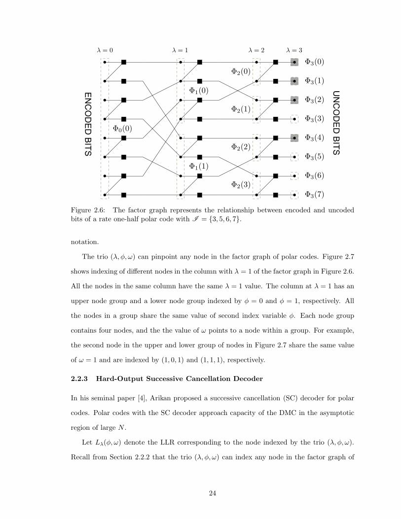
ITS
EN
CO
DE
D B
ITS
Figure 2.6: The factor graph represents the relationship between encoded and uncodedbits of a rate one-half polar code with I = 3, 5, 6, 7.
notation.
The trio (λ, φ, ω) can pinpoint any node in the factor graph of polar codes. Figure 2.7
shows indexing of different nodes in the column with λ = 1 of the factor graph in Figure 2.6.
All the nodes in the same column have the same λ = 1 value. The column at λ = 1 has an
upper node group and a lower node group indexed by φ = 0 and φ = 1, respectively. All
the nodes in a group share the same value of second index variable φ. Each node group
contains four nodes, and the the value of ω points to a node within a group. For example,
the second node in the upper and lower group of nodes in Figure 2.7 share the same value
of ω = 1 and are indexed by (1, 0, 1) and (1, 1, 1), respectively.
2.2.3 Hard-Output Successive Cancellation Decoder
In his seminal paper [4], Arikan proposed a successive cancellation (SC) decoder for polar
codes. Polar codes with the SC decoder approach capacity of the DMC in the asymptotic
region of large N .
Let Lλ(φ, ω) denote the LLR corresponding to the node indexed by the trio (λ, φ, ω).
Recall from Section 2.2.2 that the trio (λ, φ, ω) can index any node in the factor graph of
24

(1,0,0)
(1,0,1)
(1,0,2)
(1,0,3)
(1,1,0)
(1,1,2)
(1,1,3)
(1,1,1)
Figure 2.7: The trio (λ, φ, ω) can index all the nodes in the factor graph of polar codes.
polar codes.
Figure 2.7 explains Lλ(φ, ω) notation for LLRs corresponding to the nodes in the factor
graph of polar codes. Figure 2.7 shows only the nodes for the column with λ = 1 of the
factor graph in Figure 2.6. Since all the LLRs belong to the same column, their notation
has the same form L1(·, ·). As explained in Section 2.2.2, φ corresponds to the node group
and ω corresponds to the node within the node group Φλ(φ). All the LLRs of the upper
node group Φ1(0) have the same form L1(0, ·), as all of them have the same φ = 0 value.
Similarly, all the LLRs of the lower node group Φ1(1) have the same form L1(1, ·). Within
a node group, the LLR of an individual node is denoted using ω. For example in Figure 2.7,
L1(1, 2) denotes the LLR of the third node from the top in the lower group of nodes Φ1(1).
Let Bλ(φ, ω) denote the bit decision corresponding to the node indexed by the trio
(λ, φ, ω).
Let us denote the memory used to store LLRs and bit decisions corresponding to all the
nodes in the factor graph as L and B, respectively.
The SC decoder detects the message bits using Algorithms 2.1, 2.2 and 2.3. Algorithm
2.1 wraps up the SC decoder initializing L0(0, i)(N−1)i=0 with LLRs received from the channel
and iterates through all the message bits u in the outer loop. If the message bit corresponds
to the frozen bit, the algorithm sets message decision Bn(i, 0) to zero. Otherwise, Algorithm
2.1 calls Algorithm 2.2 to compute LLR Ln(i, 0) of ui and decides about Bn(i, 0) based
25

Algorithm 2.1: The SC decoder
Data: LLRs from channelResult: Message Estimates in Bn(i, 0)(N−1)
i=0
1 L0(0, i)(N−1)i=0 ← LLRs from channel
2 for i = 0→ (N − 1) do3 if i ∈ I c then4 Bn(i, 0) ← 05 end6 else7 updatellrmap(n, i)8
Bn(i, 0)←
0 if Ln(i, 0) > 0,
1 otherwise.(2.11)
9 end10 if i is odd then updatebitmap(n, i)
11 end
on Ln(i, 0). Algorithm 2.2 calculates LLR Ln(i, 0) for ui using the estimates for already
detected bits. For all message bits, Algorithm 2.1 calls Algorithm 2.3 if the message bit
being detected has an odd index, e.g., u3, u5 etc. Algorithm 2.3 keeps on updating the
decisions for all nodes in the factor graph recursively as the decoder detects the message
bits.
In these algorithms, ⊞ is defined as
(2.10)a⊞ b , 2 tanh−1
[
tanh(a
2
)
× tanh
(b
2
)]
.
2.3 The Construction of Polar Codes
The basic principle of the construction of polar codes is to find a set I such that the block
error probability of the polar code is minimum when decoded using the SC decoder. Arikan
provided an upper bound on the block error probability of polar codes under the SC decoder
[4] as follows:
Pe ≤∑
i∈I
Pe(i), (2.17)
where Pe(i) is the error probability in detecting ui given the perfect knowledge of all the
previous bits u0 to ui−1 and no information about ui+1 to uN−1 – the bits yet to be detected.
26
Algorithm 2.2: updatellrmap(λ, φ)
1 if λ = 0 then return
2 ψ ← ⌊φ2 ⌋3 if φ is even then updatellrmap(λ− 1, ψ)
4 for ω = 0→(2n−λ − 1
)do
5 if φ is even then6
Lλ(φ, ω)← Lλ−1(ψ, 2ω) ⊞ Lλ−1(ψ, 2ω + 1) (2.12)
7 end8 else9 if Bλ(φ− 1, ω) is 0 then
10
Lλ(φ, ω)← Lλ−1(ψ, 2ω + 1) + Lλ−1(ψ, 2ω) (2.13)
11 end12 else13
Lλ(φ, ω)← Lλ−1(ψ, 2ω + 1)− Lλ−1(ψ, 2ω) (2.14)
14 end
15 end
16 end
Algorithm 2.3: updatebitmap(λ, φ)
1 if φ is odd then2 for ω = 0→
(2n−λ − 1
)do
3
Bλ−1(ψ, 2ω) ← Bλ(φ− 1, ω)⊕Bλ(φ, ω) (2.15)
Bλ−1(ψ, 2ω + 1)← Bλ(φ, ω) (2.16)
4 end5 if ψ is odd then updatebitmap(λ− 1, ψ)
6 end
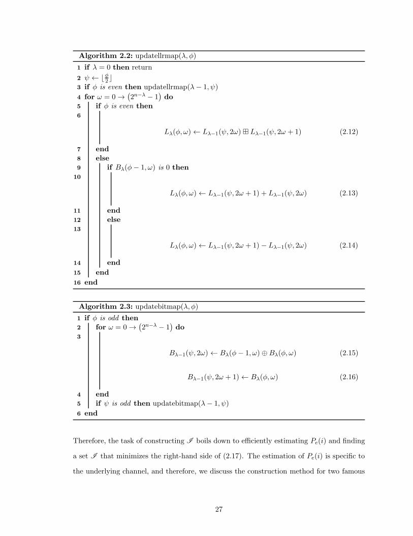
Therefore, the task of constructing I boils down to efficiently estimating Pe(i) and finding
a set I that minimizes the right-hand side of (2.17). The estimation of Pe(i) is specific to
the underlying channel, and therefore, we discuss the construction method for two famous
27

channels; namely, the binary erasure channel (BEC) and the added white Gaussian noise
(AWGN) channel.
2.3.1 Construction for the BEC
Suppose we want to construct a polar code for a BEC with erasure probability ǫ. Arikan
showed in [4] that we can calculate Pe(i) = ǫn(i) using the following recursions:
ǫk(2j) = 2ǫk−1(j) − ǫ2k−1(j),
ǫk(2j + 1) = ǫ2k−1(j),
where ǫλ(φ) represents the erasure probability for the bits corresponding to Φλ(φ) and
ǫ0(0) = ǫ. The last step of the code construction is to choose a set I such that∑
i∈IPe(i)
is minimum.
2.3.2 Construction for the AWGN Channel
For more general channels (including the AWGN channel), [4], [1], [14], and [15] constitute
a list for the methods to estimate Pe(i). In this thesis, we choose the method reported in
[1] because of its accuracy and implementation ease.
The method of [1] is an extension of the full-blown density evolution-based construction
[14] and assumes Gaussian distribution for the LLRs exchanged. In this method, we
suppose that the transmitter sends all-zeros codeword. In the case of all-zeros codeword
transmission, it is easy to show that the log-likelihoods (LLRs) 2ri/σ2 are distributed
according to a Gaussian distribution with mean 2/σ2 and variance 4/σ2, i.e., 2ri/σ2 ∼
N (2/σ2, 4/σ2). Since the decoder uses the same equations to compute all the LLRs in a
Φλ(φ), all these LLRs follow the same distribution N (mλ(φ), 2mλ(φ)), where mλ(φ) is the
mean of this distribution. In this notation, the LLRs corresponding to message bits ui have
mean mn(i), and the probability of error Pe(i) (the probability that the LLR is negative)
is given by:
Pe(i) = Q
(√
mn(i)
2
)
. (2.18)
Trifonov and Semenov showed in [1] that mn(i) in (2.18) can be approximated using the
28

initial value of m0(0) = 2/σ2 in the following recursions:
mk(2j) = g(mk−1(j)),
mk(2j + 1) = 2mk−1(j),
(2.19)
where
g(x) = h−1(
1− (1− h(x))2)
, (2.20)
h(x) =
e−0.4527x0.86+0.0218 x > 10,
√πxe
−x4
[1− 10
7x
]otherwise.
Once we have Pe(i) for all i ∈ 0, 1, . . . , N − 1, we can choose a set I that minimizes
∑
i∈IPe(i) in (2.17).
2.4 System Model
The binary codeword v is interleaved and mapped to x ∈ 1,−1N . x is passed through
an ISI channel with impulse response h = [h0h1, . . . , hµ−1] followed by the AWGN channel
with noise variance σ2 = N0/2, so that kth element of observation r at the output of the
channel is
rk =
µ−1∑
i=0
hixk−i + nk, (2.21)
where nk ∼ N (0, σ2) is a Gaussian random variable with mean zero and variance σ2. The
per-bit signal-to-noise ratio is thus Eb/N0 =∑
i hi2/(2Rσ2), where R = K/N .
The receiver uses a standard turbo equalization architecture. It equalizes the channel
using the Bahl, Cocke, Jelinek and Raviv (BCJR) algorithm [16], computes extrinsic
log-likelihoods (LLRs) eb using BCJR, deinterleaves eb to ab and passes the result to
the polar decoder that estimates the message vector m as well as the extrinsic LLRs ed.
Extrinsic LLRs ed are interleaved again and are passed to the BCJR equalizer which uses
these LLRs as prior information to once again compute eb. This information/LLR exchange
continues for T number of iterations and at the end of the last iteration, the message vector
m is estimated.
29

2.5 Advanced Decoders for Polar Codes
Arikan showed that polar codes achieve capacity with the SC decoder in the asymptotic
region of very large block length [4]. For finite block lengths, the SC decoder is not an
optimal decoder for polar codes, and since [4], many advanced decoders have been proposed,
most of which are hard-output decoders. In this section, we review three most important
of the advanced decoders for polar codes that outperformed the SC decoder.
2.5.1 Hard-Output Successive Cancellation List Decoder
The SC decoder is a greedy algorithm that estimates bit ui in ascending order, and once
the decoder decides about a bit, it does not go back to correct the bit in case of an incorrect
decision. The SC decoder uses the bit’s decision for the decision of all subsequent bits, and
as a result, the effect of an incorrect decision propagates to all the subsequent decisions.
Tal and Vardy proposed a successive cancellation list (SCL) decoder that alleviates the
error propagation problem of the SC decoder by keeping both the options of ui being zero
and ui being one. The two options for every bit being detected results in a list of possible
sequences of the size exponential in the number of bits detected instead of only one sequence
as in the case of the SC decoder. Since, this exponential increase in the number of sequences
require a large amount of memory, the decoder uses a pruning technique. In the pruning
technique, when the number of possible sequences in the list increases beyond a preset size
L, the least probable sequences are dropped from the list, and in the end, the SCL decoder
chooses the sequence with the largest likelihood as the estimated sequence.
The difference between the SC decoder and the SCL decoder is explained in Figure 2.8.
Both of these decoders can be described with the help of a tree diagram. In this tree
diagram, each node represents a sequence of decisions, and the number next to each node
represents its probability. The root node represents an empty sequence with probability
one, as it points to the start of the decoding process. As the decoding proceeds, the tree
starts building up from root node to leaf nodes. The first bit to decide is u0. A branch
to the left represents a u0 = 0 decision, while a branch to the right represents a u0 = 1
decision. The task of any sequential decoder, starting from the detection of u0 to that of
30
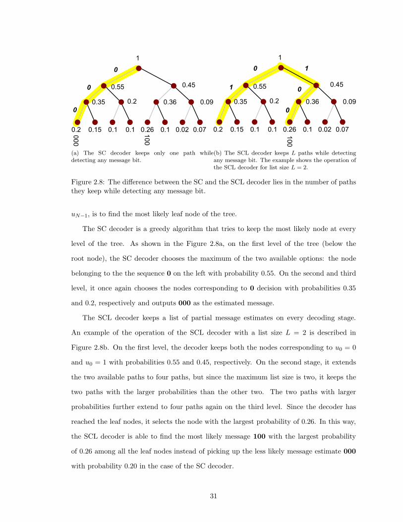
(a) The SC decoder keeps only one path whiledetecting any message bit.
(b) The SCL decoder keeps L paths while detectingany message bit. The example shows the operation ofthe SCL decoder for list size L = 2.
Figure 2.8: The difference between the SC and the SCL decoder lies in the number of pathsthey keep while detecting any message bit.
uN−1, is to find the most likely leaf node of the tree.
The SC decoder is a greedy algorithm that tries to keep the most likely node at every
level of the tree. As shown in the Figure 2.8a, on the first level of the tree (below the
root node), the SC decoder chooses the maximum of the two available options: the node
belonging to the the sequence 0 on the left with probability 0.55. On the second and third
level, it once again chooses the nodes corresponding to 0 decision with probabilities 0.35
and 0.2, respectively and outputs 000 as the estimated message.
The SCL decoder keeps a list of partial message estimates on every decoding stage.
An example of the operation of the SCL decoder with a list size L = 2 is described in
Figure 2.8b. On the first level, the decoder keeps both the nodes corresponding to u0 = 0
and u0 = 1 with probabilities 0.55 and 0.45, respectively. On the second stage, it extends
the two available paths to four paths, but since the maximum list size is two, it keeps the
two paths with the larger probabilities than the other two. The two paths with larger
probabilities further extend to four paths again on the third level. Since the decoder has
reached the leaf nodes, it selects the node with the largest probability of 0.26. In this way,
the SCL decoder is able to find the most likely message 100 with the largest probability
of 0.26 among all the leaf nodes instead of picking up the less likely message estimate 000
with probability 0.20 in the case of the SC decoder.
31

Polar codes outperform LDPC codes if concatenated with a CRC code and decoded
by the SCL decoder with a minute difference from above-mentioned algorithm [5]. The
difference is that at the end of the decoding operation, the sequence that passes CRC check
is picked up instead of picking up the sequence with largest probability.
2.5.2 Hard-Output Simplified Successive Cancellation Decoder
One of the drawbacks of the SC decoder is its very high latency: approximately 0.5fR [8],
where f is the clock frequency. To overcome this problem, Alamdar-Yazdi and Kschischang
proposed the SSC decoder that exploited the rate-zero and rate-one subcodes in a polar
code [11]. A rate-zero subcode is the one that does not transmit any information, and all
its message bits are fixed to zero. On the other hand, a rate-one subcode is the one that
does not provide any error-correcting capability, and all its message bits are free bits. For
example, in Figure 2.6 the subgraph consisting of Φ3(0),Φ3(1) and Φ2(0) correspond to
a rate-zero subcode, because no information is transmitted using this subcode as all the
nodes belonging to this subcode are fixed to zero. Similarly, the subgraph consisting of
Φ3(6),Φ3(7) and Φ2(3) correspond to a rate-one subcode, because both Φ3(6) and Φ3(7)
correspond to free bits.
The SSC decoder skips the computations for rate-zero subcodes (corresponding to frozen
bits), and decodes rate-one subcodes (corresponding to free bits) in one clock cycle using
the thresholding operation. In this way, the decoder avoids unnecessary computations and
reduces the computational complexity as well as decoding latency.
For example, consider the SSC decoder operation to decode a polar code of N = 8 and
I = 3, 5, 6, 7 as shown in Figure 2.6. The SSC decoder starts with the computation
of L3(0), i.e., the top node at the depth λ = 3, but the decoder knows a-priori that the
nodes at (3, 0, 0) and (3, 1, 0) correspond to fixed bits and fixes B2(0) to zero. Therefore,
the decoder can skip the calculation of L3(0),L(1) and L2(0) and directly assign bit
decisions in B2(0) to zero. The decoder computes L1(0) and proceeds to the calculation of
L3(2),L3(3) as usual. In a similar way to rate-zero subcodes, the nodes (3, i, 0)7i=6 form
a rate-one sub-code. In [11], the authors proposed skipping the calculation of L3(i)7i=6
32

and computing B2(3) by thresholding the LLRs in L2(3) using an operation like (2.11)
in Algorithm 2.1. In this way, the SSC decoder reduces the number of operations, and
therefore, reduces the latency in the decoder.
2.5.3 Soft-Output Belief Propagation Decoder
The factor graph description of Figure 2.6 enables the message passing based BP algorithm
to be used for polar codes [17], [18]. One advantage of this decoder is that it provides
soft outputs for the coded bits. The pitfall, however, is that it requires a large number
of iterations over the factor graph of the polar code resulting in a larger processing and
memory requirement. Additionally, a large number of iterations hinders high-throughput
(low-latency) implementations. Therefore, this high processing, memory and latency
requirement of the BP decoder makes it practically infeasible for many applications. We
briefly describe the operation of the decoder here.
The decoder works locally on protographs of length two by computing extrinsic LLRs
corresponding to all the four nodes of the protograph. Figure 2.9 explains the LLR updates
in a single protograph, which is the factor graph of a polar code of length two. The
decoder first updates L1(0, 0) using L0(0, 0) and L0(0, 1) from L and B1(1, 0) from B, and
then updates B1(1, 0) using the same L0(0, 0) and L0(0, 1) from L but B1(0, 0) from B,
completing the left-to-right update on the protograph. The decoder then starts to update
the LLRs from right to left by updating B0(0, 0) and B0(0, 1). The four steps shown in
Figure 2.9 complete the updates on this single protograph. The LLRs in red represent the
LLRs that are used to update the LLRs in green.
The BP decoder updates messages on the top-right protograph of the factor graph and
then moves down updating all the protograph at λ = n. Once the BP decoder has updated
all the protographs at depth λ = n, it moves from right to left updating all the protographs
at depth 0 ≤ λ < n in a similar fashion until it reaches the bottom-left corner of the factor
graph, completing the first iteration of the BP decoder. The decoder repeats this process for
a fixed number of iterations and at the end of last iteration, produces the message estimate.
33

Figure 2.9: The BP decoder updates LLRs on a protograph-by-protograph basis. In asingle protograph, it updates four LLRs with two LLRs in both L and B.
Since the BP decoder is the only soft-output decoder available for polar codes, we
compare its performance metrics with those of the BP decoder for LDPC codes. Figure 2.10
compares the trade-off between the complexity and the Eb/N0 required to achieve FER =
10−3 on a dicode channel with impulse response h = [ 1 − 1 ]. The total number of
turbo iterations between the channel detector and the decoder is 15. The number next to
an individual performance point refers to the number of iterations used in the respective
decoder. The LDPC code used is an irregular LDPC code of the variable node distribution
λ(x) = 0.2184x+0.163x2 +0.6186x3, check node distribution ρ(x) = 0.6821x4 +0.3173x5 +
0.0006x6, average column weight dv = 3.4 and row weight dc = 5.31. Clearly, the BP
decoder for polar codes requires a larger number of computations and Eb/N0 to achieve the
required FER than that for LDPC codes. The BP decoder for polar codes with 60 iterations
require approximately 11 times more iterations than the BP decoder for LDPC codes with
60 iterations. The huge computational complexity overshadows any benefits polar codes
have and makes polar codes with BP decoder infeasible for practical applications.
The BP decoder for polar codes requires 2N(log2(N) + 1) real values to store, whereas
full parallel implementation of the BP decoder for LDPC codes requires storage of N(dv+1)
34

106
107
108
2
2.5
3
3.5
4
4.5
5
No. of Operations
Pola
r - BP
30
40
60
1020 30 40
LDPC - BP
Figure 2.10: The polar code with BP decoding performs worse than the LDPC code withBP decoding on both the fronts: it requires a larger number of computations while requiringa larger Eb/N0 to achieve FER = 10−3 on a dicode channel.
[19] real values. Figure 2.11 shows the relative memory required for the BP decoder for
LDPC codes with respect to the one required for that for polar codes, and for block lengths
of practical importance (N > 2048) is well below 15%.
Unlike the computational complexity and memory requirement, latency is highly related
to the hardware implementation of a decoder, and it is hard to compare two decoders until
they are realized in hardware. The hardware implementation of a decoder is beyond the
scope of this thesis, but if we are able to reduce the number of operations required to
be performed in a sequential fashion, we can guarantee latency reduction by reducing the
clock cycles required to perform these operations without any hardware implementation.
An excellent example is the SSC decoder we described in Section 2.5.2 in which the decoder
skips the detection of a few bits that used to occur in a sequential order in the SC decoder,
35

0 2 4 6 8 10 12 14 160
0.5
1
1.5
2
2.5
LD
PC
-BP
Mem
ory
/Po
lar-
BP
Me
mory
Figure 2.11: The BP decoder for LDPC codes requires less than 50% of the memoryrequired by BP decoder for polar codes with N > 16. This relative memory requirementdecreases monotonically and goes very low for practical block lengths such as only 13% fora code of length 32768.
resulting in a lower number of clock cycles required. In this thesis, we will be concerned
with the latency improvement resulting from these methods based on reducing the number
of sequential operations required instead of hardware implementation.
36

CHAPTER III
IMPROVED BELIEF-PROPAGATION SCHEDULE FOR POLAR
CODES
Chapter 2 briefly discussed the BP decoder, which provides the soft outputs needed for
turbo-based receivers as well as better performance than the SC decoder. However, these
gains come at the price of high complexity and latency of the decoder that render it infeasible
for practical applications. In this chapter, we take the first step toward the ideal system by
proposing a decoder based on a new schedule that targets this high complexity issue.
In the original BP decoder, the message updates follow a flooding schedule, in which
it updates messages on a protograph-by-protograph basis starting from the top-right
protograph and coming down till the bottom-right one. The decoder repeats the same
process for all the depths of the factor graph completing its first iteration. After the
first iteration, the decoder repeats the same process for a fixed number of iterations. As
explained later in detail, the flooding schedule is unable to disseminate the information
efficiently throughout the factor graph and requires many iterations to reach acceptable
error rates.
We propose a new serial schedule based on the successive cancellation schedule of the
SC decoder and call it the soft-cancellation schedule. We call the message-passing decoder
with the proposed schedule the soft-cancellation SCAN decoder. The proposed schedule
reduces the complexity of the decoder immensely compared to the flooding schedule of the
BP decoder and is similar to the schedule of message updates in the SC decoder. Therefore,
the ideas used in the improvement of the SC decoder can be extended to the SCAN decoder
in many cases. Furthermore, we propose a technique to reduce memory utilization of the
decoder based on the proposed schedule.
We now explain the key idea behind the proposed schedule.
37

Figure 3.1: System model for Lemma: 3.1
3.1 The Soft-Cancellation (SCAN) Schedule and Decoder
Consider the factor graph of a polar code of length two as shown in Figure 3.1. We call the
small factor graph the basic decision element, as in the SC decoder, all the processing on the
factor graph of any polar code of length more than two occurs locally on this basic decision
element. Therefore, we can build our intuition and analysis of the proposed schedule on the
basic decision element and then extend it to the general case of the factor graph of polar
codes with length larger than two.
Suppose we encode the bits u0, u1 using a polar code of length two and map the resulting
coded bits to x0, x1 ∈ +1,−1. We then send x0 and x1 on a binary-input DMC W with
transition probabilities W (y|x). The SC decoder first calculates the log-likelihood ratio for
the bit u0 using (2.12) with channel observations y0, y1 while assuming that u1 is equally
likely to be 0 or 1. The SC decoder assumes this about u1, because it does not have
an estimate of u1 yet. Once it has an estimate for the bit u0, it assigns the estimate to
B1(0, 0) using (2.11) and calculates the log-likelihood ratio for the bit u1 using (2.13) with
the assumption that u0 has been decoded with no error. After the calculation of m1 using
L1(1, 0) in (2.11), it assigns m1 to B1(1, 0) and use (2.12) to estimate the values of x0, x1.
The final operation of assigning m1 completes the SC decoding on this polar code of length
two.
The aforementioned process transforms the vector channel W2(y0, y1|u0, u1) into two
separate channels W−SC and W+
SC defined by the transition probabilities W−SC(y0, y1|u0) and
38

W+SC(y0, y1, u0|u1), respectively. We reiterate the assumptions used in the SC decoder as
follows:
1. u1 is equally likely to be 0 or 1 for the computation of likelihood W−SC(y0, y1, u1|u0).
2. u0 has been decoded with no error for the computation of likelihood
W+SC(y0, y1, u0|u1).
The first assumption is an oversimplification given the channel observations y0 and y1
contain information about u0 that the decoder is not using, whereas the second assumption
is true only for very high Eb/N0. Both assumptions degrade the LLR estimates, and we
expect improved LLR estimates if we can incorporate soft information about u0 and u1
in the decoder instead of hard decision and no information, respectively. We first show in
the following lemma how the likelihood computation changes if we have access to such soft
information, and then we show how we provide this soft information in the SCAN decoder.
Figure 3.1 explains the system model used in this lemma. We encode bits u0 and u1
to x0 and x1 and transmit on channel W . At the receiver, the SC decoder has y0 and
y1 as channel observations to estimate the transmitted bits. Now assume that we have
information about u0 and u1 through other channels P0 and P1 in the form of z0 and z1,
respectively. Lemma 3.1 describes the likelihood calculations for u0 and u1 given access to
y0, y1, z0 and z1.
Lemma 3.1. Let z0 and z1 be the output of DMCs P0 and P1, defined by the transition
probabilities P0(z0|u0) and P1(z1|u1), respectively. Suppose z0 and z1 are conditionally
independent given u0 and u1, respectively implying P (z0, z1|u0, u1) = P0(z0|u0)P1(z1|u1).
If we have access to z0 or z1 instead of perfect or no knowledge of u0 and u1, respectively
the log-likelihood ratios of u0 and u1 are given by
L1(0, 0) = L0(0, 0) ⊞ [B1(1, 0) + L0(0, 1)] , (3.1)
L1(1, 0) = L0(0, 1) + [B1(0, 0) ⊞ L0(0, 0)] . (3.2)
Proof. The proof is provided in the Appendix A.
39

One problem that remains now is to show how we can provide additional LLRs
B1(0, 0), B1(1, 0) in all decision elements in a factor graph for any N . In the start of a
decoding cycle, we compute L0(0, k)(N−1)k=0 as we receive symbols r from the channel.
We inform the decoder about the location of fixed bits by initializing Bn(k, 0)k∈I c to
∞. Suppose we are interested in finding the LLR Ln(i, 0) with Ln(k, 0)(i−1)k=0 already
computed and no information about ukN−1k=(i+1)
. Since we cannot have any information
about ukN−1k=(i+1) in the first iteration, we will keep the assumption that they are equally
likely, i.e., Bn(k, 0) = 0,∀(i + 1) ≤ k ≤ (N − 1). It is noteworthy that we have already
populated L partially from left to right while calculating Ln(k, 0)(i−1)k=0 . Therefore, as we
calculate Ln(k, 0)(i−1)k=0 , we can use the partially calculated L as a-priori information to
update B from right to left using (3.1) and (3.2) on all the decision elements involved. When
i = N − 1, we have B with extrinsic LLRs corresponding to all the nodes in the decoder’s
factor graph.
We once again start computing LLRs Ln(i, 0)N−1i=1 , but this time we have soft
information in B for ukN−1k=(i+1) unlike the first iteration. Therefore, we can use B to supply
a-priori information to all decision elements in subsequent iterations. We use this iterative
process I times and use the extrinsic LLRs Ln(i, 0)N−1i=0 and B0(0, i)N−1
i=0 calculated in
the last iteration corresponding to message and coded bits, respectively. We explain all the
necessary implementation details in Algorithms 3.1, 3.3 and 3.2.
Algorithm 3.1 provides the decoder’s wrapper and calls Algorithm 3.2 to calculate
Ln(φ, 0)(N−1)φ=0 . Algorithm 3.2 updates L from left to right using B as prior information.
Since B is initialized to zero except Bn(i, 0)(N−1)i=0 , Bλ(φ+1, ω) in Algorithm 3.1 has zero
value in the first iteration, just like the SC decoder. On the other hand, the SCAN decoder
in the first iteration uses soft information in Bλ(φ − 1, ω) in contrast to the SC decoder
which uses hard information about Bλ(φ − 1, ω) in (2.13). As we iterate through φ in the
inner loop of Algorithm 3.1, for the odd values of φ the wrapper calls Algorithm 3.3 to
update B from right to left. Algorithm 3.3 populates B using L as prior information, and
by the end of the first iteration, B0(0, φ)(N−1)φ=0 contains extrinsic LLRs for the coded bits.
In the second iteration, (3.3) uses the values of Bλ(φ+ 1, ω) from the first iteration, unlike
40

the first iteration in which Bλ(φ + 1, ω) were initialized to zero. Algorithm 3.1 repeats
this process for I times using the outer loop and estimates message bits at the end of Ith
iteration.
One of the important parameters of polar codes under any decoding scheme is the
rate of channel polarization, which describes how fast the capacity of the transformed bit
channels approaches 1 and 0, respectively as N →∞. We refer the interested readers to [4]
for further details about this parameter, and mention here the advantage of using the SC
decoder in place of the SCAN decoder with I = 1 for the AWGN channel. We observe that
by clipping the LLRs of already detected bits to +∞,−∞ we can increase the convergence
and polarization rate. Zimmermann et al. [20] observed the same phenomenon in belief
propagation decoder for LDPC codes and called it ’belief pushing ’. It is noteworthy here
that the SCAN decoder with I = 1 is different from the SC decoder, because the SC decoder
clips the LLRs of already detected bits in the factor graph to either +∞ or −∞, whereas
the SCAN decoder uses soft information about these bits. However, both of these decoders
do not use information about the bits yet to be detected and are similar in this respect.
With this in mind, one can convert the SCAN decoder with I = 1 into the SC decoder
by assigning Bn(k, 0) =∞× sgn(Bn(k, 0) +Ln(k, 0)) as we calculate Ln(k, 0)N−1k=0 , where
sgn(.) is the sign function. Therefore, we can consider the SC decoder as a modified version
of the more general SCAN decoder. We conclude this section by presenting the following
proposition.
Proposition 3.1. The rate of channel polarization is higher under the SC decoder than the
SCAN decoder with I = 1.
Proof. The proof is provided in the appendix.
3.2 Reducing the Memory of the SCAN Decoder
One of the two contributors to the area and power consumption on a chip is memory as
explained in Section 1.4. A larger memory requirement translates into a higher power and
area utilization, and therefore, the memory requirement of a decoder should be minimized as
41

Algorithm 3.1: The SCAN decoder
1 initialization
2 L0(0, i)(N−1)i=0 ← LLRs from channel
3 Bn(i, 0)i∈I c ←∞4 Bn(i, 0)i∈I ← 0
5 Bλ(φ)n−1λ=0 ← 0, ∀φ ∈ 0, . . . , 2λ − 1
6
7 for i = 1→ I do8 for φ = 0→ (N − 1) do9 updatellrmap(n, φ)
10 if φ is odd then updatebitmap(n, φ)
11 end
12 end13 for i = 0→ (N − 1) do14 if (Bn(i, 0) + Ln(i, 0)) ≥ 0 then mi ← 015 else mi ← 1
16 end
Algorithm 3.2: updatellrmap(λ, φ)
1 if λ = 0 then return
2 ψ ← ⌊φ2 ⌋3 if φ is even then updatellrmap(λ− 1, ψ)
4 for ω = 0→(2n−λ − 1
)do
5 if φ is even then6
Lλ(φ, ω)← Lλ−1(ψ, 2ω) ⊞ [Lλ−1(ψ, 2ω + 1) +Bλ(φ+ 1, ω)] (3.3)
7 end8 else9
Lλ(φ, ω)← Lλ−1(ψ, 2ω + 1) + [Lλ−1(ψ, 2ω) ⊞Bλ(φ− 1, ω)] (3.4)
10 end
11 end
much as possible. In this section, we propose a technique to reduce the memory requirement
of the SCAN decoder.
In [5] and [8], a memory-efficient version of the SC decoder has been proposed by
modifying L and B memory indexing. The proposed modifications reduced the memory
requirement for L and B to 2N−1 and 4N−2, respectively. We show that the modification
42

Algorithm 3.3: updatebitmap(λ, φ)
1 if φ is odd then2 for ω = 0→
(2n−λ − 1
)do
3
Bλ−1(ψ, 2ω)← Bλ(φ− 1, ω)⊞ [Bλ(φ, ω) + Lλ−1(ψ, 2ω + 1)] (3.5)
Bλ−1(ψ, 2ω + 1)← Bλ(φ, ω) + [Bλ(φ− 1, ω)⊞ Lλ−1(ψ, 2ω)] (3.6)
4 end5 if ψ is odd then updatebitmap(λ− 1, ψ)
6 end
that [5] proposed for L can be directly applied to the SCAN decoder, and the memory
requirement for L can be reduced to 2N − 1 from N(n + 1). On the other hand, the
modification that [5] proposed for B is not directly applicable for the reasons explained later.
This section introduces a partitioning method for B that reduces its memory requirement
to 4N − 2 +Nn/2 from N(n+ 1).
We first briefly describe the modification proposed for L and apply it directly to the
SCAN decoder. Looking at the factor graph in Figure 3.2, it is clear that all the Φ-groups
on a single λ depth has the same number of nodes 2n−λ. Let us denote L and B values
corresponding to Φλ(φ) as Lλ(φ) and Bλ(φ), respectively. As we calculate Ln(i, 0)N−1i=0 ,
traversing i in ascending order, we use the Φ-groups at different depths in ascending order
as well. With this schedule of LLR update, when we are updating Lλ(i), we do not need
any of the Lλ(φ) : φ < i. Therefore, we can overwrite the values of previously calculated
Lλ(φ) : φ < i and only need 2n−λ memory locations for a depth λ. Figure 3.2 shows that
the memory for Lλ(0) of size 2n−λ can be used to store all Lλ(φ) at the depth λ. Hence,
the total number of memory elements required by L is∑n
λ=0N/2λ = 2N − 1.
The SCAN decoder updates L with a similar schedule to the schedule of updates in the
SC decoder, and therefore, the above-mentioned modification can be directly applied to L
in the SCAN decoder, reducing the memory requirement of L from N(n+1) to 2N − 1. It
is noteworthy that this modification is not possible in the similar fashion to the originally
proposed belief propagation decoder of [17] because of the flooding schedule of LLR updates
in L and B.
43

Figure 3.2: At any depth λ ∈ 0, 1, . . . , n, Lλ(φ) for all φ ∈ 0, . . . , 2λ are stored in thememory for Lλ(0), which is shown in green.
The modification for B in [5] (where B used binary values) that is similar to the
modification for L described above, is not applicable to the SCAN decoder, because now
not only do we need to calculate LLRs in B, but we also need to pass them onto the next
iteration. Therefore, as [5] suggested for the SC decoder, we cannot overwrite the values of
B.
To see how we might reduce the memory requirement for B in the SCAN decoder, we
first present the following notation and lemmas. Consider Lλ(φ) and Lλ(δ) at any depth
λ,∀φ 6= δ and φ, δ ∈ 0, . . . , 2λ − 1.
We denote
Lλ(φ) ≺ Lλ(δ)
to show that the decoder updates Lλ(φ) before Lλ(δ).
Lemma 3.2. At any depth λ ∈ 0, . . . , n, the SCAN decoder updates Φ-groups for both L
44

and B in ascending order from φ = 0→ N − 1, i.e.,
Lλ(φ) ≺ Lλ(φ+ 1)
Bλ(φ) ≺ Bλ(φ+ 1)
for all φ ∈ 0, . . . , 2λ − 2.
Proof. We prove this lemma using mathematical induction. First we note the following
trivial cases:
1. The SCAN decoder does not update B and L for λ = n and λ = 0.
2. The SCAN decoder trivially updates B in ascending order for λ = 0, because there is
only one Φ-group.
3. The SCAN decoder trivially updates L in ascending order for λ = n because of the
schedule of the decoder on this depth.
First we prove this Lemma for L only. Let us denote φλi 2λ
i=0 as the sequence in which
we update L at any depth λ. From the schedule of the SCAN decoder, we know that
φni = i2ni=0. Suppose that φki = i2ki=0 is true. From (3.3) and (3.4), we know that the
update in Lλ(φ) requires the update in Lλ−1(⌊φ/2⌋). Therefore, φ(k−1)i = i2k−1
i=0 is also
true from the definition of the ’floor’ function. We can use the same argument for both the
base and induction step of the proof.
Similarly, with (3.5) and (3.6), we can prove the same results for B.
Lemma 3.3. At any depth λ ∈ 1, . . . , n− 1,
Lλ(φ) ≺ Bλ(φ) ≺ Lλ(φ+ 1), (3.7)
where φ ∈ 0, . . . , 2λ − 2.
Proof. Without loss of generality, consider the calculation of Lλ(φ) and Lλ(φ + 1) for φ
even, and λ ∈ 2, . . . , n. From Lemma 3.2, (3.3) and (3.4) we know that
Lλ−1(ψ) ≺ Lλ(φ) ≺ Lλ(φ+ 1),
45

where ψ = ⌊φ/2⌋. Also from (3.5) and (3.6),
Lλ(φ+ 1) ≺Bλ−1(ψ).
Therefore, using these two relationships we get
Lλ−1(ψ) ≺ Bλ−1(ψ).
Now considering the calculation of Lλ(φ+ 2) and Lλ(φ+ 3), we get
Lλ−1(ψ + 1) ≺ Bλ−1(ψ + 1).
From Lemma 3.2, we know that at any λ, the decoder updates both L and B in ascending
order, we conclude
Lλ−1(ψ) ≺ Bλ−1(ψ) ≺ Lλ−1(ψ + 1),
for all λ ∈ 2, . . . , n, and ψ ∈ 0, . . . , 2λ−1 − 2. We complete the proof by changing
variables.
Theorem 3.1. In any iteration i and for any depth λ, the SCAN decoder requires only
Bλ(φ) : φ is odd from iteration (i− 1) to update L.
Proof. Consider (3.3) for iteration i. From Lemma 3.3, we know that
Lλ(φ) ≺ Bλ(φ).
Therefore, when the decoder is updating Lλ(φ), Bλ(φ+1) is holding the value from iteration
(i − 1). Since it is true for φ even only, (φ + 1) is odd and we use Bλ(i) : i is odd from
(i − 1). Similarly, (3.4) shows that to update Lλ(φ) for odd φ, we need Bλ(φ − 1) that,
by Lemma 3.3, the decoder has already updated.Therefore, Bλ(φ − 1) contains the values
calculated in the current iteration i.
Suppose we reserve two separate memory locations for B: one to hold Bλ(φ) :
φ is even, namely E and one for Bλ(φ) : φ is odd, namely O. From Theorem 3.1,
we conclude that we only need to keep O for the next iteration with only N/2 elements at a
46

depth λ. In contrast, the decoder will use E in the current iteration only, and therefore the
decoder can use the same space Bλ(0) for all Bλ(φ), φ is even at a depth λ by overwriting
it. The number of memory elements required for E is exactly the same as required for L,
i.e., (2N − 1).
The decoder also needs to specify the indexing of both E and O. As noted in [5], φ
does not convey any information in indexing memory location for any Lλ(φ), because the
decoder writes all the values to the same location Lλ(0). Since E is similar to L in the
sense that the SCAN decoder does not need E from one iteration to the other, the decoder
can use the same indexing for both E and L. One such memory indexing function is
f(λ, ω) = ω + 2(n+1) − 2(n+1−λ). (3.8)
Since O is used only for odd values of φ, we can convert these odd values into the natural
numbers by a simple transformation and then use it to index O. One such indexing function
is
g(λ, φ, ω) = ω + (φ− 1)2(n−λ−1) + (λ− 1) 2(n−1). (3.9)
Figure 3.3 presents a small example of a rate-1/2 polar code. In this example, the SCAN
decoder reuses B2(0) and B3(0) (shown with green rectangles) by overwriting them with
the values of B2(2),B3(2),B3(4) and B3(6), and does not need extra memory for them.
On the other hand, the SCAN decoder keeps the values for Bλ(φ),∀λ, φ is odd as they
are required for the next iteration.
We summarize the details of the proposed low-complexity SCAN decoder in Algorithm
3.4, 3.5 and 3.6. Algorithm 3.4 is the top-level wrapper for the SCAN decoder, similar to
Algorithm 3.1. The SCAN decoder successively calls Algorithm 3.5 and 3.6 as it traverses
all the uncoded bits from i = 0 to N − 1. Algorithm 3.6 updates the two portions of B
using L as prior information: E for the groups with φ even and O for the groups with φ
odd, whereas Algorithm 3.5 updates L using E and O as prior information. It is noteworthy
that in all the algorithms we have indexed E and O using (3.8) and (3.9), respectively.
47

Figure 3.3: Memory elements required to store B with corresponding φ displayed next to aparticular Bλ(φ). In any iteration, the SCAN decoder does not need Bλ(φ) : φ is even forthe next iteration, and we can overwrite Bλ(0) (shown with green rectangles) at any depthλ with Bλ(φ) : φ is even, φ 6= 0 (shown with yellow rectangles). On the other hand, theSCAN decoder requires Bλ(φ) : φ is odd (shown with white rectangles) for processing inthe next iteration, and therefore it will keep these memory locations as they are. In thissmall example, we save five memory elements corresponding to B2(2),B3(2),B3(4) andB3(6).
3.3 A Comparison with the Flooding Schedule
In this section, we compare the flooding schedule of the BP decoder with the SCAN schedule
using Figure 3.3.
Consider first the operation of the BP decoder on the factor graph shown in Figure 3.3.
Just like the SCAN decoder, the BP decoder also uses two memory locations L and
B. The decoder starts by updating LLRs L3(0, 0), L3(1, 0), B2(0, 0) and B2(0, 1) using
L2(0), B3(0, 0) and B3(1, 0). In this way, the decoder updates the LLRs corresponding to
the top-right protograph and then repeats the same process for all the four protographs
under λ = 2. After the updates in the protographs under λ = 2, the decoder updates the
48

Algorithm 3.4: The SCAN decoder with reduced memory requirement
Result: Extrinsic LLRs E0(0, ω)N−1ω=0
1 L0(0, i)(N−1)i=0 ← LLRs from channel
2 On(i, 0)i∈I c,i is odd ←∞3 for i = 1→ I do4 for φ = 0→ (N − 1) do5 updatellrmap(n, φ)6 if φ is even then7 if φ ∈ I c then Em(φ, 0)←∞8 else Em(φ, 0)← 0
9 end10 else updatebitmap(n, φ)
11 end
12 end
Algorithm 3.5: updatellrmap(λ, φ)
1 if λ = 0 then return
2 ψ ← ⌊φ2 ⌋3 if φ is even then updatellrmap(λ− 1, ψ)
4 for ω = 0→(2n−λ − 1
)do
5 if φ is even then Lλ(φ, ω)← Lλ−1(ψ, 2ω) ⊞ [Lλ−1(ψ, 2ω + 1) + Eλ(φ+ 1, ω)]6 else Lλ(φ, ω)← Lλ−1(ψ, 2ω + 1) + Lλ−1(ψ, 2ω) ⊞Oλ(φ− 1, ω)
7 end
four protographs under λ = 1 and then λ = 0 completing its first iteration. The following
points are noteworthy in this schedule:
1. The BP decoder updates L and B on a protograph-by-protograph basis.
2. In any iteration to update any LLR in both L and B, the BP decoder uses the values
in B that are updated in the current iteration and the values in L updated in the
previous iteration (or in the case of first iteration, the initialized values of L).
3. When the BP decoder is updating the LLRs under λ = 0 at the end of the
first iteration, the information received from the channel in L0(0) moves from the
protographs under λ = 0 to the protographs under λ = 1. Therefore, in the first
iteration the information from the fixed bits travels from the right-most end of the
factor graph to the left-most end, but the information received from the channel moves
only to the neighboring protographs, i.e., the protographs under λ = 1. Following
49

Algorithm 3.6: updatebitmap(λ, φ)
1 ψ ← ⌊φ2 ⌋2 if φ is odd then3 for ω = 0→
(2n−λ − 1
)do
4 if ψ is even then5
Eλ−1(ψ, 2ω)← Eλ(φ− 1, ω)⊞ [Oλ(φ, ω) + Lλ−1(ψ, 2ω + 1)]
Eλ−1(ψ, 2ω + 1)← Oλ(φ, ω) + Eλ(φ− 1, ω)⊞ Lλ−1(ψ, 2ω)
6 end7 else8
Oλ−1(ψ, 2ω) ← Eλ(φ− 1, ω)⊞ [Oλ(φ, ω) + Lλ−1(ψ, 2ω + 1)]
Oλ−1(ψ, 2ω + 1)← Oλ(φ, ω) + Eλ(φ− 1, ω)⊞ Lλ−1(ψ, 2ω)
9 end
10 end11 if ψ is odd then updatebitmap(λ− 1, ψ)
12 end
the same procedure, we can show that in every iteration, the information about the
fixed bits traverses the whole factor graph, whereas the information received from the
channel moves to the neighboring protographs only, and it requires n iterations to
reach the right-most end of the factor graph.
The SCAN decoder updates L1(0), L2(0), L3(0) and L3(1) in this order. After the
update in L3(1), the SCAN decoder updates B2(0) using L2(0) that has just been updated.
In this way, as the SCAN decoder updates L3(i) from i = 0 to 7, it populates B using the
updated values in L. At the end of the first iteration, the information received from the
channel moves from left end of the factor graph to the right while the information about
the fixed bits move from the right end to the left. The following points are noteworthy in
this schedule:
1. The SCAN decoder does not update L and B on protograph-by-protograph basis;
instead it is a node-by-node basis update schedule except in the protographs under
λ = 2. For example, the SCAN decoder first updates L1(0), L2(0), L3(0) that are
50
the updates corresponding to the top-right node of the protographs involved.
2. In any iteration to update any LLR in B, the SCAN decoder uses B as well as L
updated in the current iteration. To update any LLR in L, the decoder uses L and
Bλ(φ) : φ even updated in the current iteration while Bλ(φ) : φ odd updated
in the previous iteration.
3. In any iteration, the information about both the fixed bits in B3(i)7i=0 and the
information received from the channel in L0(0) traverse the entire factor graph.
As described above, the BP decoder needs at least n iterations to disperse the information
contained in Bn(i)(N−1)i=0 and L0(0) in the entire factor graph, whereas the SCAN decoder
achieves this with only one iteration. In this way, the SCAN decoder achieves a faster
convergence by better disseminating the information in the factor graph than the BP
decoder, as pointed out by the last two points of the schedules in both the decoders.
3.4 Performance Results
In this section, we compare the error-rate performance of the SCAN decoder with the SC
decoder and the BP decoder for polar codes, and the BP decoder for LDPC codes.
3.4.1 The AWGN Channel
Figure 3.4 demonstrates the improved performance of our algorithm in the AWGN channel.
We have simulated the SC and the SCAN decoder for a polar code of block length N = 32768
and dimension K = 16384. The polar code is optimized for Eb/N0 = 2.35 dB in the AWGN
channel using the method of [1]. The design Eb/N0 = 2.35 dB is obtained by sweeping
design Eb/N0 for a range of values and picking up the one that resulted in the best FER
performance. We have simulated a maximum of 106 frames to calculate error rates on all
Eb/N0 values, terminating the simulation if 100 or more frames are found in error.
In terms of frame error rates, the SCAN decoder with one iteration performs worse than
the SC decoder. The worse performance is in agreement with Proposition 3.1, as the rate
of polarization for the SCAN decoder with only one iteration is lower than that of the SC
decoder. By clipping the LLRs for already detected bits to extreme values of infinity, the
51

SC decoder converges faster than the SCAN decoder with one iteration. However, with
only two iterations, the SCAN decoder outperforms the SC decoder, providing a gain of 0.1
dB in the required Eb/N0 for a frame error rate of 10−4. Further increase in the number of
iterations of the SCAN decoder to four does not provide any significant gain.
In contrast to the FER performance, the SCAN decoder with only one iteration
has better bit error rate (BER) performance than that of the SC decoder. The better
performance of the SCAN decoder is due to the fact that in case of incorrect decoding,
the SC decoder converges to an incorrect but valid codeword, because it produces hard bit
decisions for message bits that combined with frozen bits has one-to-one correspondence
with a codeword in the code. Therefore, whenever the SC decoder is unable to decode a
message, it produces at least dmin errors, where dmin is the minimum Hamming distance
of the code and is usually a large number for powerful codes. Recall that the Hamming
distance between two codewords is the number of positions in which the two codewords
differ, and the minimum Hamming distance dmin of a code is the minimum Hamming
distance between any two codewords of the code. In contrast to the SC decoder, the SCAN
decoder does not have the restriction of converging to a valid codeword in case of decoding
failure. The SCAN decoder, by nature, is a distributed algorithm, and its codeword decisions
may not correspond to message decisions at all, because they belong to different parts of
the factor graph. The SCAN decoder’s bit error rate performance improves even further
with increasing number of iterations, and with only two iterations, provides approximately
0.2 dB gain to achieve FER=10−4. With four iterations, the SCAN decoder’s performance
saturates and does not improve any further with increasing number of iterations.
3.4.2 Partial Response Channels
Figure 3.5 shows the performance of the SCAN decoder on the dicode channel for a polar
code of length N = 8192 and dimension K = 4096 under turbo equalization architecture
[6]. We have designed the polar code using the method of [1] for the AWGN channel with
Eb/N0 = 1.4 dB. The design Eb/N0 = 1.4 dB is obtained by calculating FER corresponding
to a range of design Eb/N0 values and picking up the one that resulted in the best FER. In
52

1 1.2 1.4 1.6 1.8 210
−5
10−4
10−3
10−2
10−1
100
BER
FER
SCAN I =
1
SC
AN
I =1
Arik
an's S
C
Arikan's SC
SCAN I =
2SCAN I =
4
SCAN I =
2
SCAN I =4
Figure 3.4: FER and BER performance of the SCAN decoder in the AWGN channel forN = 32768. We have optimized the polar code for Eb/N0 = 2.35 dB using the method of[1].
all simulations, a maximum of 15 turbo iterations are used.
The SCAN decoder with only two iterations outperforms the BP decoder with 60
iterations on the dicode channel, where the complexity of one iteration of both the decoders
is the same. With further increase in number of iterations, the performance improves, and
with only eight iterations the SCAN decoder provides about 0.3 dB gain in the required
Eb/N0 over the BP decoder to achieve FER= 10−3.
Figure 3.5 also shows the performance of the SCAN decoder on the EPR4 channel for
a polar code of length N = 8192 and dimension K = 4096, designed using the method of
[1] for the AWGN channel with Eb/N0 = 1.55 dB. The design Eb/N0 is obtained by the
same Eb/N0 sweeping for a range of values as used for the dicode channel. The SCAN
decoder shows the same performance improvement over the BP decoder for polar codes as
53

shown in the dicode channel, and with only two iterations, performs comparable to the BP
decoder with 60 iterations in the EPR4 channel. With eight iterations, the SCAN decoder
provides about 0.2 dB gain in the required Eb/N0 over the BP decoder for polar codes with
60 iterations to achieve FER= 10−3.
We also compare the polar code’s performance with the SCAN decoder to that of an
irregular LDPC code of the variable node distribution λ(x) = 0.2184x+0.163x2 +0.6186x3,
check node distribution ρ(x) = 0.6821x4+0.3173x5+0.0006x6, average column weight dv =
3.4 and row weight dc = 5.31 decoded using the BP algorithm and constructed using [21],
[22] and [23]. The performance difference between this LDPC code with the BP algorithm
and the polar code with the SCAN decoder (using four iterations) is approximately 0.3 dB
for FER = 10−3 on the dicode channel. The performance loss in the case of the EPR4
channel is larger than that in the case of the dicode channel.
Furthermore, it has been shown that polar codes outperform LDPC codes if
concatenated with very simple codes [5], [24] in the AWGN channel. In this respect, the
SCAN decoder can have potential applications for turbo decoding of concatenated codes
because of their ability to provide soft outputs.
3.5 Complexity Analysis
Table 1 compares the complexity of the BP decoder for LDPC codes with that of the BP and
the SCAN decoder for polar codes. We have used the complexity analysis for LDPC codes
given in [25], where one iteration consists of variable-to-check and then check-to-variable
message passing. We have further assumed that the decoder uses table lookup method to
calculate both tanh(.) and tanh−1(.).
The processing requirement of the SCAN decoder with two iterations is only 4% of that
of the BP decoder with 60 iterations for polar codes while both of the decoders deliver
approximately the same frame error rate performance in both the dicode and the EPR4
channel. With eight iterations, the SCAN decoder has processing requirement of only
13% of that of the BP decoder with 60 iterations but has gain in the required Eb/N0 of
approximately 0.3 dB and 0.2 dB to achieve FER = 10−3 in the dicode and the EPR4
54

Figure 3.5: FER performance of the SCAN decoder in partial response channels for K =4096 and N = 8192. We have optimized the polar code for Eb/N0 = 1.4 dB (dicode) andEb/N0 = 1.55 dB (EPR4) using the method of [1].
channels, respectively.
The number of operations required for the SCAN decoder with four iterations is
approximately equal to 60% of that required for the BP decoder for the LDPC code with
50 iterations. The complexity reduction comes at the price of higher Eb/N0 requirement to
achieve the same error-rate performance, as shown in Figure 3.5.
Figure 3.6 shows how the normalized memory requirement of the SCAN decoder with
respect to the BP decoder for polar codes decreases with the increase in n. The BP decoder
uses N(n+ 1) real memory elements for each of L and B. The SCAN decoder uses 2N − 1
and 4N − 2 + Nn/2 real memory elements for L and B, respectively. Figure 3.6 shows
that the memory required by the SCAN decoder at two practical frame lengths of 4096
and 32768 is 43% and 39% of that required by the BP decoder, respectively. In summary,
55

Table 1: Complexity Comparison of Different Decoders
Complexity/Iteration
Operation LDPC BP Polar SCAN/BP
Table Lookups (N −K)(dc + 1) 6Nn
Multiplications (N −K)(dc − 1) 2Nn
Divisions (N −K)dc 0
Additions/Subtractions 2Ndv 2Nn
Total Operations 5Ndv 10Nn
2 4 6 8 10 12 14 16 18
0.4
0.5
0.6
0.7
0.8
0.9
1
Figure 3.6: Memory efficiency improves with increasing block length.
the SCAN decoder requires approximately half the memory required by the BP decoder for
polar codes for practical block lengths.
3.6 Summary
In this chapter, we have introduced SCAN, a soft-output decoder for polar codes that
offers good performance, low computational complexity and low memory requirements. The
56

proposed decoder achieves its complexity reduction by adopting a serial schedule instead
of a flooding schedule of the BP decoder. The SCAN decoder’s computational complexity
with two iterations is approximately 4% that of the BP decoder with 60 iterations on the
dicode channel, with comparable performance. Furthermore, the SCAN decoder requires
Nn/2 (unlike N(n + 1) for the BP decoder) memory elements to pass from one iteration
to the next. Using this fact, a memory-splitting method is proposed in which the decoder
keeps one portion of the memory needed for the next iterations as it is and optimizes the
other one that it uses in the current iteration. With the proposed modification, the memory
required by the SCAN decoder is approximately 39% of that required by the BP decoder
at a block length N = 32768 in one example.
57

CHAPTER IV
AN ENHANCED SCAN DECODER WITH HIGH THROUGHPUT
AND LOW COMPLEXITY
In this chapter, we propose an enhanced SCAN (eSCAN) decoder that outperforms the
SCAN decoder of the previous chapter in the following ways: computational complexity,
latency and memory usage.
In the previous chapter, we showed that changing the schedule of message updates in
the BP decoder drastically reduces the complexity of soft-output decoding of polar codes.
Although the new serial schedule reduces the complexity of the decoder, its serial nature
severely hampers the decoder’s throughput. The SC decoder faces the same problem,
because its schedule for message update is the same as the SCAN decoder. Fortunately,
for the SC decoder a number of techniques have been proposed to reduce this high latency
problem, and many of them are directly applicable to the SCAN decoder. One of these
techniques is the simplified successive cancellation (SSC) decoding of Alamdar-Yazdi and
Kschischang [11]. However, a direct implementation of the SSC principle to the SCAN
decoder requires large memory and the knowledge whether LLRs in different parts of the
factor graph are fixed to ∞, zero or take value from R.
In this chapter, we prove that the location of frozen bits exhibit structural properties
for a class of polar codes that provide the knowledge about LLR values in different parts of
the factor graph of a polar code. The class of polar codes include the ones constructed for
binary erasure channel using Arikan’s method [4] and the AWGN channel using Gaussian
approximation based density evolution [1]. The proposed properties define the structure of
the complete factor graph of a polar code using just the location of frozen bits, and thus help
in the extension of the SSC principle to the SCAN decoder, reducing the SCAN decoder’s
latency and computational complexity. In addition to the application of the SSC principle
to the SCAN decoder, we also propose a technique based on the structural properties to
58

reduce the memory requirement of the SCAN decoder. The memory reduction is in addition
to the reduction in the computational complexity and the latency of the SCAN decoder that
come from the application of the SSC principle.
The structure of the chapter is as follows. Section 4.1 introduces the structural properties
of polar codes and Section 4.2 provides an intuitive explanation for these properties.
In Section 4.3, we apply these properties to propose a memory-efficient, low-complexity
and low-latency enhanced SCAN (eSCAN) decoder. Section 6.2.2 analyzes the proposed
hight-throughput low-complexity SCAN decoder.
4.1 The Properties of Polar Codes
One can construct the generator matrix for any (N,K,R) polar code by first taking the
Kronecker power of a kernel matrix of small dimension (such as 2×2 in the case of classical
polar codes [4]) and then removing N − K rows of the matrix by fixing corresponding
message bits to zero. The construction of polar codes is explained in depth in Section 2.3.
The Kronecker power introduces a pattern in the structure of both the encoder and
decoder which is a very desirable feature from hardware implementation perspective as it
generally reduces area utilization and wiring congestion [7]. On the other hand, the location
of frozen bits does not show any pattern whatsoever.
The construction of polar codes consists of specifying the location of frozen bits. Arikan
proposed a DE-based technique to construct polar codes for the BEC only. Mori and
Tanaka employed DE to construct polar codes for the AWGN channel [14], but the method
is limited to moderate block lengths as the complexity of DE is very high. Trifonov and
Semenov [1] approximated DE of [14] by assuming Gaussian distribution on the messages
exchanged in the factor graph. Tal and Vardy approached this construction problem using
channel upgradation/degradation [15] principles.
In this section, we prove that in the class of polar codes constructed using density
evolution (DE) for the BEC and Gaussian assumption based DE [1] for the AWGN
channel, only a few patterns of the location of fixed bits are possible. The patterns in
the location of fixed bits force some node groups in the factor graph to take zero, infinity
59

or real log-likelihoods, thereby reducing the processing from a node-by-node basis to a
group-by-group basis. We also identify these patterns in the entire factor graph, and as an
application, exploit these patterns for an efficient implementation of a fast low-complexity
soft-output decoder for polar codes. Specifically, if we pair two consecutive bit locations
in the detection order of the SC decoder, then either both of the bits are fixed, free or the
fixed bit precedes the free bit. We further prove that patterns similar to the ones in the
location of fixed bits emerge in the entire factor graph of a polar code under the SCAN
decoder. In general, any pair of consecutive node groups at any depth in the factor graph
are restricted to a few patterns based on whether LLRs corresponding to all the nodes in
individual node groups of the pair are zero, ∞ or from R.
Now we will formally introduce and prove the properties of the polar codes constructed
using the method of [1]. The proofs for the case of the BEC are identical and are skipped.
At this point, we urge the reader to revisit Section 2.3 to refresh the notation and the
concepts related to the construction of polar codes. The following proofs and explanation
will heavily rely on Section 2.3.
Let
Bλ(φ) η denotes Bλ(φ, ω) ∈ η, for all ω ∈ 0, 1, . . . , 2λ − 1.
For η ∈ 0, ∞, we can interpret the notation as ‘will stick to’, e.g., Bλ(φ) 0
implies that all the elements in Bλ(φ) will stick to zero for all the iterations of the decoder.
We first prove two lemmas for the construction method of [1] described in Section 2.3.2.
Lemma 4.1.
2x− x2 > x2, for 0 < x < 1.
Proof.
x > x2 =⇒ 2x > 2x2 =⇒ 2x− x2 > x2.
Lemma 4.2.
2x > x > g(x), for 0 < x < 1,
60
where g(.) is defined in (2.20).
Proof.
2x > x = h−1(h(x)) = h−1(2h(x) − h(x)).
Since h(x) is monotonically decreasing and h(x) < 1,
2x > x > h−1(2h(x) − h(x)2) = h−1(1− (1− h(x))2) = g(x).
Consider values in B corresponding to the basic protograph in the upper-right corner
of Figure 4.1 that builds the entire factor graph of a polar code. This protograph has
two inputs on the right and two outputs on the left. We call the sets from which these
inputs and outputs take value the input and the output set, respectively. Table 2 shows all
possible input sets for this protograph, corresponding output sets and a distinct ID for the
protograph based on input/output sets. We use Pi as the designator for the protograph
with ID i.
Given a design set I , let p(Pi) denotes the probability (in the frequentist sense) of
protograph Pi appearing at depth λ = n.
Theorem 4.1 (Special Prohibited Pairs Property).
p(Pi) = 0, for i ∈ 3, 4, 5, 6, 7, 8. (4.1)
Proof. We know from Line 3 and 4 in Algorithm 3.1 that the decoder initializes B by
assigning infinity and zero LLRs at depth λ = n corresponding to fixed and free bits,
respectively. From the SCAN decoder operation, we know that it does not update these
LLRs in the entire decoding process. Therefore, for the entire decoding process, Bn(i)N−1i=0
has elements either from 0 or ∞. Mathematically,
Bn(i)N−1i=0 0 or ∞.
61

Table 2: Protograph Input/Output Set Relationship
Protograph ID Input Output
0 ∞ ∞ ∞ ∞1 ∞ 0 R R
2 0 0 0 03 ∞ R R R
4 R 0 R R
5 R R R R
6 0 ∞ 0 ∞7 0 R 0 R
8 R ∞ R ∞
Figure 4.1: Only P0, P1 and P2 are possible at depth n in the factor graph of the polarcodes. The inputs on the right of these three protographs specify whether bit is free (incase of 0) or fixed (in case of ∞). In case of P0, P1 and P2, both of the output nodeshave LLRs from the same set. For example for P0, the values in B0(0) corresponding toboth the output nodes on the left have LLRs from the set ∞, i.e., the LLRs in both ofthese nodes are stuck to ∞. On the other hand in P6, LLRs corresponding to output nodescome from the set 0,∞, i.e., both the values are different unlike other three protographs.
62

Therefore, p(Pi) = 0 is trivially true for all i ∈ 3, 4, 5, 7, 8, because all these protographs
have R as either of their input sets, and R is not possible as an input set at depth n.
Therefore, we only need to prove the theorem for i = 6.
Recall from Section 2.3.2 that for the construction method based on Gaussian
assumption, LLRs in Lλ(φ) have Gaussian distribution with mean mλ(φ) and variance
2mλ(φ). Using the recursions in (2.19), we know that for any given mn−1(φ) and for all
φ ∈ 0, 1, . . . , N/2 − 1,
mn(2φ+ 1) = 2mn−1(φ)
> g (mn(φ))
= mn(2φ). (4.2)
We can convert the relationship between two mean values mn(2φ+ 1) and mn(2φ) in (4.2)
into a relationship between the probability of error in (2φ)th and (2φ+1)th bit, respectively
as follows:
Pe(2φ) = Q(√
mn(2φ)/2)
> Q(√
mn(2φ + 1)/2) Q(.) is monotonically decreasing
= Pe(2φ+ 1). (4.3)
It is shown in (2.17) of Section 2.3 that to construct a polar code, we need to construct a
set of free indices I such that∑
i∈IPe(i) is minimized. To minimize the sum, we need
to include the bits with lowest error probabilities to I . Therefore, we will never pick
(2φ+1)th node as fixed bit compared to (2φ)th bit for all φ ∈ 0, 1, . . . , N/2− 1, because
Pe(2φ) > Pe(2φ+ 1) as proved in (4.3).
Theorem 4.1 describes the pattern in the location of fixed bits and prohibits any free
bit preceding a fixed bit in any pair of consecutive bits in the detection order of the SC
decoder.
Following theorem generalizes the result of Theorem 4.1 to rest of the factor graph.
63

Theorem 4.2 (General Prohibited Pairs Property). Let Bλ(2φ) and Bλ(2φ + 1) be two
consecutive groups at any depth λ ∈ 1, . . . , n and for any φ ∈ 0, 1, 2, . . . , 2λ−1 − 1. The
following group patterns are impossible in the polar code constructed using the method in
[1]:
1. (Bλ(2φ),Bλ(2φ+ 1)) (0, ∞).
2. (Bλ(2φ),Bλ(2φ+ 1)) (0,R).
3. (Bλ(2φ),Bλ(2φ+ 1)) (R, ∞).
Proof. We prove this theorem by contradiction. From Theorem 4.1, only protographs P0, P1
and P2 are possible at depth λ = n, and the proof is complete for λ = n. For λ = k, k ∈
1, . . . , (n− 1), we investigate all the cases separately.
1. Case 1: Let us contrary assume that two consecutive Bλ(2φ) and Bλ(2φ + 1) exist
such that (Bk(2φ),Bk(2φ + 1)) (0, ∞), for some φ ∈ 0, 1, 2, . . . , 2k−1 − 1.
The contrary assumption is true only if all the elements of X correspond to free bits,
and all the elements of Y correspond to fixed bits, where
X = 2(n−k)(2φ), . . . , 2(n−k)(2φ+ 1)− 1, (4.4)
Y = 2(n−k)(2φ+ 1), . . . , 2(n−k)(2φ+ 2)− 1. (4.5)
Mathematically,
Bn(i)
0 i ∈ X
∞ i ∈ Y. (4.6)
Figure 4.2 explains this case of the proof for k = 1 and φ = 0. For k = 1 and φ = 0,
the contrary assumption becomes (B1(0),B1(1)) (0, ∞), which implies that
all the bits in X = 0, . . . , 3 are free while all the bits in Y = 4, . . . , 7 are fixed.
Since all the elements in X and Y correspond to free and fixed bits, respectively, the
error probabilities will follow the following relationship:
Pe(i) < Pe(j), for any i ∈ X, j ∈ Y. (4.7)
64

Figure 4.2: The notation used in the proof of Theorem 4.2 is explained.
We can equivalently write (4.7) as
mn(i) ≥ mn(j), for any i ∈ X, j ∈ Y,
which implies
mini∈X
mn(i) ≥ maxj∈Y
mn(j). (4.8)
By repeated application of Lemma 4.2, we can easily show that
mini∈X
mn(j) = mn(2(n−k)(2φ))
= go(n−k+1) (mk−1(φ)) ,
and
maxj∈Y
mn(i) = mn(2(n−k)(2φ+ 2)− 1)
= 2(n−k+1)mk−1(φ),
65

where go(j) denotes the j-times application of the function g(x). So, (4.8) becomes,
go(n−k+1) (mk−1(φ)) ≥ 2(n−k+1)mk−1(φ).
But from repeated application of Lemma 4.2 on mk−1(φ), we have
go(n−k+1) (mk−1(φ)) < 2(n−k+1)mk−1(φ).
Therefore, our original assumption is wrong, and no such case exists.
2. Case 2: Let us contrary assume that two consecutive Bλ(2φ) and Bλ(2φ + 1) exist
such that (Bk(2φ),Bk(2φ + 1)) (0, R), for some φ ∈ 0, 1, 2, . . . , 2k−1 − 1.
This implies that all the bits in X and at least one bit in Y are free bits, where X
and Y are as defined in (4.4) and (4.5). Equivalently,
mn(i) ≥ mn(j), for any i ∈ X, at least one j ∈ Y,
which implies
mini∈X
mn(i) ≥ minj∈Y
mn(j). (4.9)
By repeated application of Lemma 4.2, we can easily show that
mini∈X
mn(i) = mn(2(n−k)(2φ))
= go(n−k)(mk(2φ)),
and
minj∈Y
mn(i) = mn(2(n−k)(2φ+ 1))
= go(n−k)(mk(2φ+ 1)),
where go(j) denotes the j-times application of the function g(x). So, (4.9) becomes,
go(n−k)(mk(2φ)) ≥ go(n−k)(mk(2φ+ 1)).
Since g(.) is a monotonically increasing function and mk(2φ + 1) > mk(2φ), we have
go(n−k)(mk(2φ)) < go(n−k)(mk(2φ+ 1)),
that is a contradiction. Hence, no such case exists.
66

3. Case 3: Let us contrary assume that two consecutive Bλ(2φ) and Bλ(2φ + 1) exist
such that (Bk(2φ),Bk(2φ+1)) (R, ∞), for some φ ∈ 0, 1, 2, . . . , 2k−1− 1.
This implies that at least one bit in X is a free bit, and all the bits in Y are fixed
bits, where X and Y are as defined in (4.4) and (4.5). Equivalently,
maxi∈X
mn(i) ≥ maxj∈Y
mn(j). (4.10)
By repeated application of Lemma 4.2, we can easily show that
maxi∈X
mn(i) = mn(2(n−k)(2φ+ 1)− 1)
= 2n−k(mk(2φ)),
and
maxj∈Y
mn(i) = mn(2(n−k)(2φ+ 2)− 1)
= 2n−k(mk(2φ+ 1)).
So, (4.10) becomes,
2n−k(mk(2φ)) ≥ 2n−k(mk(2φ+ 1)).
Since mk(2φ+ 1) > mk(2φ), we have
2n−k(mk(2φ)) < 2n−k(mk(2φ+ 1)),
that is a contradiction. Hence, no such case exists.
Example 4.1. Consider a polar code with I c = 0, 1, 2, 4 and N = 8, constructed using
the method of [1] for the AWGN channel with design Eb/N0 = 2 dB. Figure 4.3 shows
the structure of the factor graph for this construction. The code has the following group
patterns:
1. (B1(0),B1(1)) (R,R).
2. (B2(0),B2(1)) (∞,R),
(B2(2),B2(3)) (R, 0).
67

3. (B3(0),B3(1)) (∞, ∞),
(B3(2),B3(3)) (∞, 0),
(B3(4),B3(5)) (∞, 0),
(B3(6),B3(7)) (0, 0).
It is clear that none of the group patterns described in Theorem 4.2 is present in the list
above.
Corollary 4.1. For any λ ∈ 0, . . . , n, φ ∈ 0, . . . , 2λ − 1,
Bλ(φ) η, η ∈ ∞, 0,R.
Proof. We prove this corollary by induction. The corollary is trivially true for the base case
of λ = n as the size of the groups is one. Suppose the corollary is true for λ = k, and we
need to show that the corollary holds for λ = k − 1. We observe from the factor graph
in Figure 4.1 that two consecutive Bλ(2φ) and Bλ(2φ + 1) combine to produce output in
Bλ(⌊φ/2⌋). Therefore, the cases in which Bλ(⌊φ/2⌋) will have mixed values are:
1. (Bk(2φ),Bk(2φ+ 1)) (0, ∞).
2. (Bk(2φ),Bk(2φ+ 1)) (0,R).
3. (Bk(2φ),Bk(2φ+ 1)) (R, ∞).
Since from Theorem 4.2, these cases are not possible, all the Bλ(φ) will either have real
values or will stick to ∞ or zero.
Equivalently, Corollary 4.1 says that all Bλ(φ) will either have real values or will stick
to zero or ∞ for the entire decoding process. It specifically removes the possibility of any
Bλ(φ) having mixed values such as from the set 0,∞.
Corollary 4.2. For any λ ∈ 0, . . . , n and φ ∈ 0, . . . , 2λ − 1, given Bλ(φ) η, where
η ∈ 0, ∞ then
Bλ(φ)
∞ if φ is even and Bλ(φ+ 1) / ∞,
0 if φ is odd and Bλ(φ− 1) / 0.
68

Proof. Assume on the contrary that for some even φ, Bλ(φ) 0. From Theorem 4.2,
Case 1 and Case 2 are not possible when φ is even. Thus, Bλ(φ) ∞. The proof for φ
odd is similar and is omitted.
Corollary 4.3. Consider Bλ(φ) for any λ ∈ 1, . . . , n with Bλ(φ) η, where η ∈
0, ∞ . For even values of φ, if Bλ(φ+ 1) / η then
Bλ(φ+ 1)
R if 2n−λ(φ+ 1) ∈ I c,
0 otherwise ,
whereas for odd values of φ, if Bλ(φ− 1) / η then
Bλ(φ− 1)
∞ if 2n−λφ− 1 ∈ I c,
R otherwise .
Proof. Consider any Bλ(φ) η, where η ∈ 0, ∞. For even values of φ, from
Corollary 4.2, we know that Bλ(φ) ∞ or Bλ(φ) R. Suppose if Bλ(φ) ∞ then
Bλ(φ+ 1) 0 ⇐⇒ Y ⊂ I =⇒ 2n−λ(φ+ 1) ∈ I ,
where Y = 2n−λ(φ+ 1), . . . , 2n−λ(φ+ 2)− 1.
Now suppose if Bλ(φ) R, then at least one element of Y should belong to I , where
Y is as defined above. Equivalently, by repeated application of Lemma 4.2,
argmini∈Y
mn(i) = 2n−λ(φ+ 1) ∈ Ic.
Similarly, for odd values of φ the proof is similar and is omitted.
Example 4.2. Consider the construction of polar code in Figure 4.3. Since B2(0) ∞
and B2(1) / ∞ with φ = 0 being even, the conditions in Corollary 4.3 are satisfied.
To know whether B2(1) 0 or B2(1) R, we only need to check if 2n−λ(φ + 1) =
23−2(0+1) = 2 ∈ I c. In this example, u2 is a fixed bit and therefore according to Corollary
4.3, B2(1) R.
69

Figure 4.3: An example design of a rate one-half polar code validates the properties. Onlyprotographs P0, P1 and P2 appear at depth λ = n (Special Prohibited Pairs Property). Inthe entire factor graph, P6, P7 and P8 do not occur (General Prohibited Pairs Property).All the node-groups have LLRs from either of the sets 0, ∞,R (Corollary 4.1).
4.2 Discussion on the Properties of Polar Codes
In this section, we discuss the rationale behind the properties derived in Section 4.1.
Figure 4.4 shows all the protographs in Table 2 except P0 and P1, along with their reduced
forms, which are similar to the ones presented by Forney [26] in the context of Reed Muller
codes. The reduced forms of protographs in Table 2 emerge from the values of LLRs in B
corresponding to the nodes on the right-hand side of these protographs.
For example, consider P1 in Figure 4.4. By using Bλ(φ − 1, ω) = ∞ and Bλ(φ, ω) = 0
in (3.5), we get
Bλ(ψ, 2ω) = Lλ(ψ, 2ω + 1),
Bλ(ψ, 2ω + 1) = Lλ(ψ, 2ω).
The aforementioned equations correspond to the reduced form of P1 shown below the
70

Figure 4.4: Every type of protograph has an equivalent reduced form.
protograph in Figure 4.4. In words, the equations show that in this protograph, two values
corresponding to Lλ(φ − 1, 2ω) and Lλ(φ − 1, 2ω + 1) go as they are in B but in swapped
locations. It is noteworthy here that LLRs in L always come from R and there is no
guarantee that these LLRs will stick to either ∞ or zero for the entire decoding process.
Since B in this protograph gets values from L, the output of the protograph shows R on
both the left nodes.
The reduced forms for P3 and P4 are an equality check code and a parity check code,
respectively. P5 is equivalent to two parity checks (note that the bottom parity check is
equivalent to an equality check). Each of P1, P3, P4 and P5 takes part in error correction
71

or checking, whereas P0 and P2 yield P1, P3, P4 and P5 under the general prohibited pair
property. Therefore, Pi, i ∈ 0, 1, . . . , 5 give rise to the error-correction capability of polar
codes.
In contrast to Pi for i ∈ 0, 1, . . . , 5, P6 and P7 result in the loss of a dimension. The
reduced forms of both of P6 and P7 are equivalent to two short-circuited upper nodes. In
the reduced form of P8, both upper and lower pair of nodes are short circuited with no
error-correction capability. In this context, we can easily conclude that the construction of
[4] and [1] discourage the ineffective protograph formations of P6, P7 and P8.
4.3 A High-Throughput, Low-Complexity Soft-Output Decoder forPolar Codes
In applications requiring large block lengths, design constraints other than error-rate
performance become stringent. The design constraints include latency, computational
complexity and storage requirement of the decoder. The latency of the decoder dictates
its throughput, whereas the higher computational complexity and storage requirement
of the decoder in general, result in higher power and area utilization in the hardware
implementation [7]. In this section, we apply the structural properties of polar codes
discussed in the previous section by proposing a memory-efficient extension of the SSC
principle to the SCAN decoder, called the enhanced SCAN (eSCAN) decoder.
We first demonstrate that like the SSC decoder, we can skip rate-one and rate-zero
subcodes in the SCAN decoder as well, and that the properties of polar codes can be
used to locate these subcodes using only I . This straightforward extension results in a
computation complexity and latency reduction as discussed in [11]. We then demonstrate
that by using the properties of polar codes discussed in Section 4.1, we can reduce the
memory utilization of the decoder in addition to the reduction in computational complexity
and latency by the application of the SSC principle. Memory utilization in the SC or the
SSC decoder is not an issue, because memory for already detected bits (in the detection
order of the SC decoder) in the factor graph is binary valued, and any further reduction or
optimization will not reduce the overall memory budget of the SC decoder. On the other
hand, in the SCAN decoder memory for both L and B is real valued, and memory reduction
72
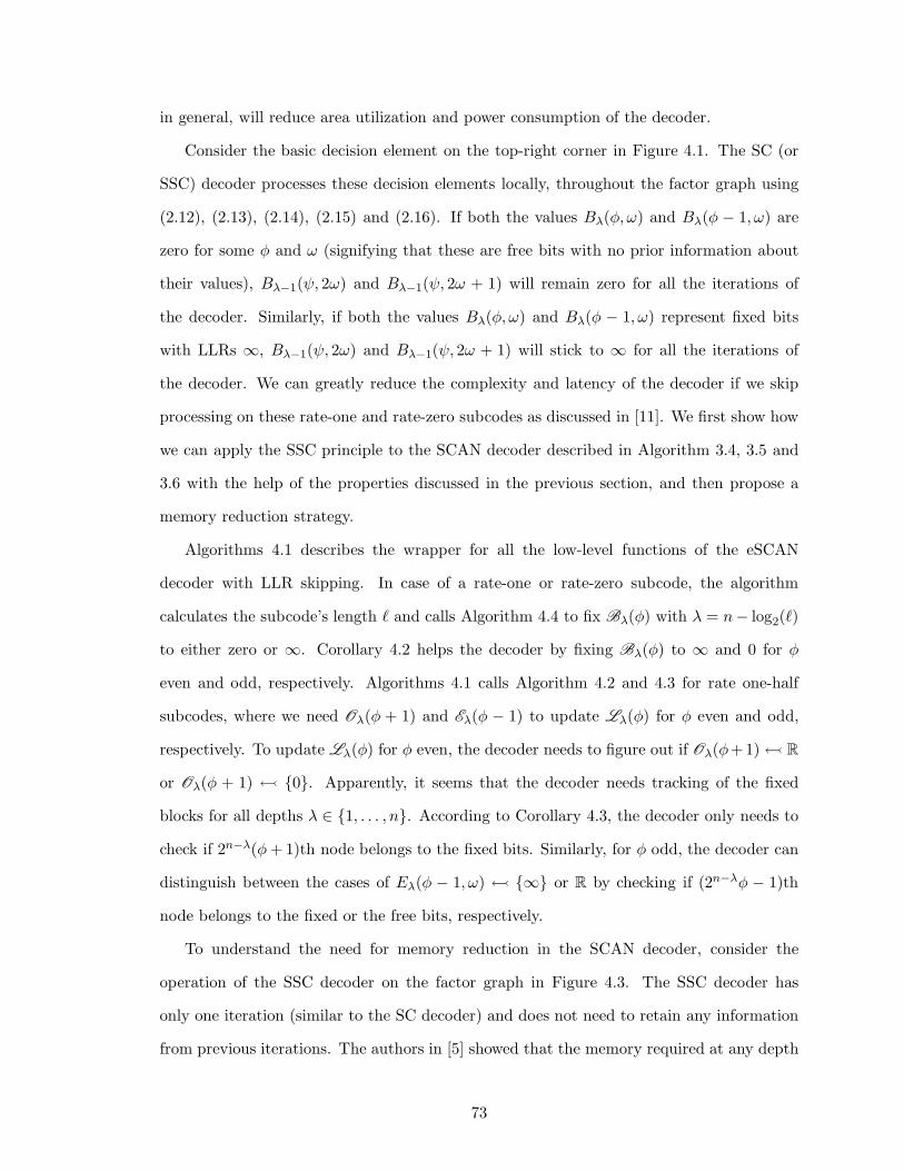
in general, will reduce area utilization and power consumption of the decoder.
Consider the basic decision element on the top-right corner in Figure 4.1. The SC (or
SSC) decoder processes these decision elements locally, throughout the factor graph using
(2.12), (2.13), (2.14), (2.15) and (2.16). If both the values Bλ(φ, ω) and Bλ(φ − 1, ω) are
zero for some φ and ω (signifying that these are free bits with no prior information about
their values), Bλ−1(ψ, 2ω) and Bλ−1(ψ, 2ω + 1) will remain zero for all the iterations of
the decoder. Similarly, if both the values Bλ(φ, ω) and Bλ(φ − 1, ω) represent fixed bits
with LLRs ∞, Bλ−1(ψ, 2ω) and Bλ−1(ψ, 2ω + 1) will stick to ∞ for all the iterations of
the decoder. We can greatly reduce the complexity and latency of the decoder if we skip
processing on these rate-one and rate-zero subcodes as discussed in [11]. We first show how
we can apply the SSC principle to the SCAN decoder described in Algorithm 3.4, 3.5 and
3.6 with the help of the properties discussed in the previous section, and then propose a
memory reduction strategy.
Algorithms 4.1 describes the wrapper for all the low-level functions of the eSCAN
decoder with LLR skipping. In case of a rate-one or rate-zero subcode, the algorithm
calculates the subcode’s length ℓ and calls Algorithm 4.4 to fix Bλ(φ) with λ = n− log2(ℓ)
to either zero or ∞. Corollary 4.2 helps the decoder by fixing Bλ(φ) to ∞ and 0 for φ
even and odd, respectively. Algorithms 4.1 calls Algorithm 4.2 and 4.3 for rate one-half
subcodes, where we need Oλ(φ + 1) and Eλ(φ − 1) to update Lλ(φ) for φ even and odd,
respectively. To update Lλ(φ) for φ even, the decoder needs to figure out if Oλ(φ+1) R
or Oλ(φ + 1) 0. Apparently, it seems that the decoder needs tracking of the fixed
blocks for all depths λ ∈ 1, . . . , n. According to Corollary 4.3, the decoder only needs to
check if 2n−λ(φ+1)th node belongs to the fixed bits. Similarly, for φ odd, the decoder can
distinguish between the cases of Eλ(φ − 1, ω) ∞ or R by checking if (2n−λφ − 1)th
node belongs to the fixed or the free bits, respectively.
To understand the need for memory reduction in the SCAN decoder, consider the
operation of the SSC decoder on the factor graph in Figure 4.3. The SSC decoder has
only one iteration (similar to the SC decoder) and does not need to retain any information
from previous iterations. The authors in [5] showed that the memory required at any depth
73

Algorithm 4.1: Low-complexity low-latency eSCAN decoder
Data: LLRs from channelResult: B0(0)
1 j ← 02 for k = 1→ J do3 for i = 0→ (N − 1) do4 if i belongs to rate-one or rate-zero subcode then5 j ← j + 16 if i is the last node of the subcode then7 ζ ← (n− log(j))8 ψ ← i/j9 j ← 0
10 fixblock(ζ, ψ)
11 end
12 end13 else14 if i is odd then15 updatellrmap(n− 1, ⌊i/2⌋)16 Bn−1(⌊i/2⌋, 1) ← Ln−1(⌊i/2⌋, 0)17 Bn−1(⌊i/2⌋, 0) ← Ln−1(⌊i/2⌋, 1)18 updatebitmap(n− 1, ⌊i/2⌋)19 end
20 end
21 end
22 end
λ for B in the SC (or the SSC) is 2(n−λ+1), i.e., the memory required for two Bλ(φ) . For
example, the SSC decoder only needs B2(0) and B2(1) for the operation at depth λ = 2.
Therefore, there is no memory requirement issue in the SSC decoder, because it already
uses a small number of memory elements at a depth λ. Additionally, since the memory
for B is of boolean type, any further optimization (if possible) will not have a significant
impact on the overall memory budget.
In case of the SCAN decoder, we have to pass on information in some of the memory
elements from one iteration to the other. The information passed on from one iteration to
the next is of real type, and can significantly impact the decoder’s memory budget. In the
memory-efficient SCAN decoder discussed in Section 3.2, we divided the memory for B in
E = Bλ(φ) : φ is even and O = Bλ(φ) : φ is odd. We further showed that only O
is required from one iteration to the other of the SCAN decoder, and E can be optimized
74
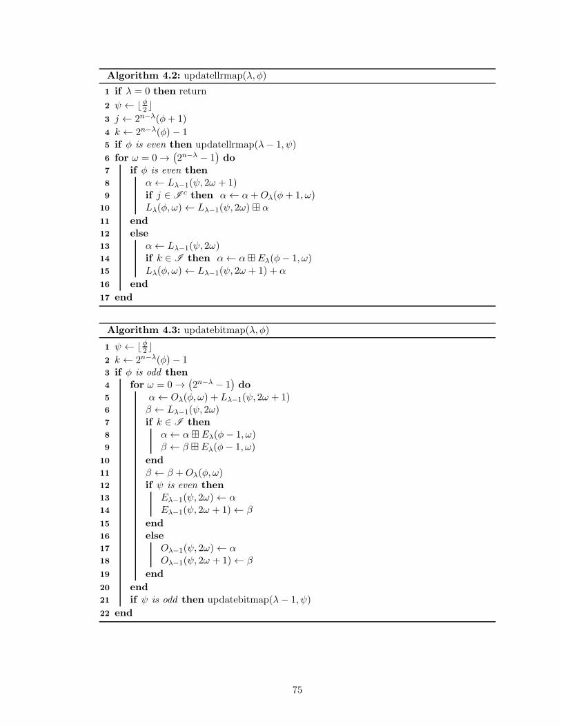
Algorithm 4.2: updatellrmap(λ, φ)
1 if λ = 0 then return
2 ψ ← ⌊φ2 ⌋3 j ← 2n−λ(φ+ 1)
4 k ← 2n−λ(φ)− 15 if φ is even then updatellrmap(λ− 1, ψ)
6 for ω = 0→(2n−λ − 1
)do
7 if φ is even then8 α← Lλ−1(ψ, 2ω + 1)9 if j ∈ I c then α← α+Oλ(φ+ 1, ω)
10 Lλ(φ, ω)← Lλ−1(ψ, 2ω) ⊞ α
11 end12 else13 α← Lλ−1(ψ, 2ω)14 if k ∈ I then α← α⊞ Eλ(φ− 1, ω)15 Lλ(φ, ω)← Lλ−1(ψ, 2ω + 1) + α
16 end
17 end
Algorithm 4.3: updatebitmap(λ, φ)
1 ψ ← ⌊φ2 ⌋2 k ← 2n−λ(φ)− 13 if φ is odd then4 for ω = 0→
(2n−λ − 1
)do
5 α← Oλ(φ, ω) + Lλ−1(ψ, 2ω + 1)6 β ← Lλ−1(ψ, 2ω)7 if k ∈ I then8 α← α⊞ Eλ(φ− 1, ω)9 β ← β ⊞ Eλ(φ− 1, ω)
10 end11 β ← β +Oλ(φ, ω)12 if ψ is even then13 Eλ−1(ψ, 2ω)← α14 Eλ−1(ψ, 2ω + 1)← β
15 end16 else17 Oλ−1(ψ, 2ω)← α18 Oλ−1(ψ, 2ω + 1)← β
19 end
20 end21 if ψ is odd then updatebitmap(λ− 1, ψ)
22 end
75
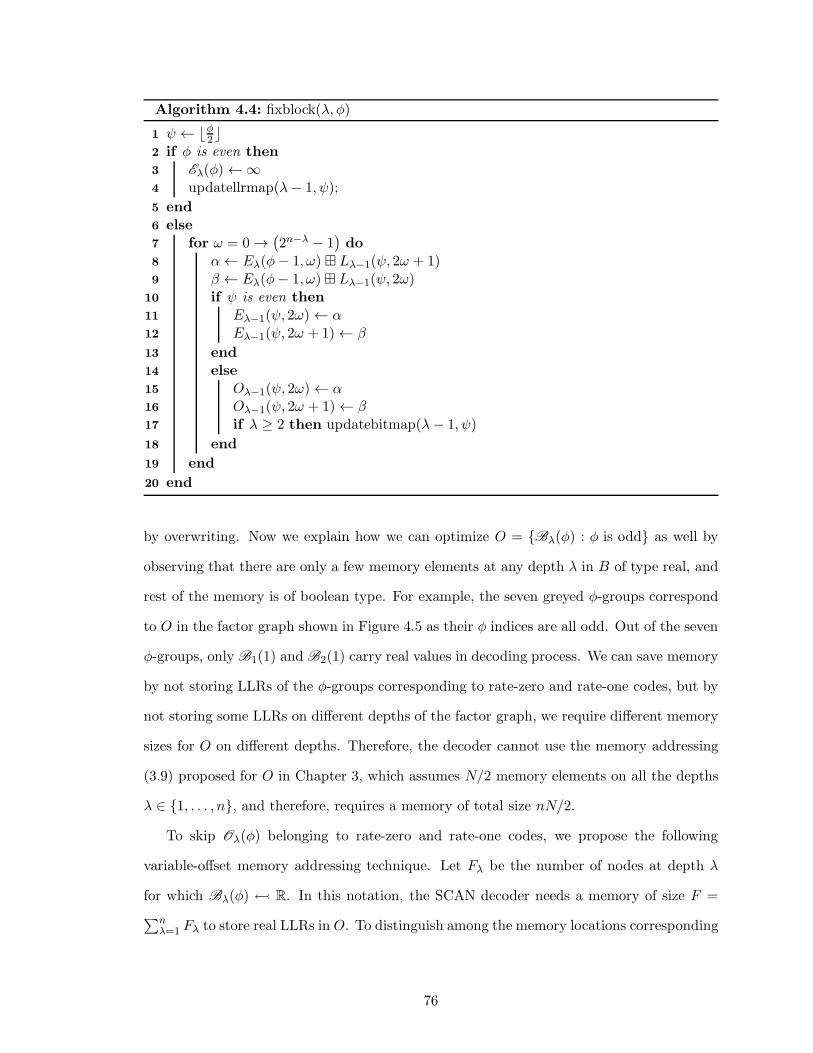
Algorithm 4.4: fixblock(λ, φ)
1 ψ ← ⌊φ2 ⌋2 if φ is even then3 Eλ(φ)←∞4 updatellrmap(λ− 1, ψ);
5 end6 else7 for ω = 0→
(2n−λ − 1
)do
8 α← Eλ(φ− 1, ω) ⊞ Lλ−1(ψ, 2ω + 1)9 β ← Eλ(φ− 1, ω)⊞ Lλ−1(ψ, 2ω)
10 if ψ is even then11 Eλ−1(ψ, 2ω)← α12 Eλ−1(ψ, 2ω + 1)← β
13 end14 else15 Oλ−1(ψ, 2ω)← α16 Oλ−1(ψ, 2ω + 1)← β17 if λ ≥ 2 then updatebitmap(λ− 1, ψ)
18 end
19 end
20 end
by overwriting. Now we explain how we can optimize O = Bλ(φ) : φ is odd as well by
observing that there are only a few memory elements at any depth λ in B of type real, and
rest of the memory is of boolean type. For example, the seven greyed φ-groups correspond
to O in the factor graph shown in Figure 4.5 as their φ indices are all odd. Out of the seven
φ-groups, only B1(1) and B2(1) carry real values in decoding process. We can save memory
by not storing LLRs of the φ-groups corresponding to rate-zero and rate-one codes, but by
not storing some LLRs on different depths of the factor graph, we require different memory
sizes for O on different depths. Therefore, the decoder cannot use the memory addressing
(3.9) proposed for O in Chapter 3, which assumes N/2 memory elements on all the depths
λ ∈ 1, . . . , n, and therefore, requires a memory of total size nN/2.
To skip Oλ(φ) belonging to rate-zero and rate-one codes, we propose the following
variable-offset memory addressing technique. Let Fλ be the number of nodes at depth λ
for which Bλ(φ) R. In this notation, the SCAN decoder needs a memory of size F =
∑nλ=1 Fλ to store real LLRs in O. To distinguish among the memory locations corresponding
76

Figure 4.5: The memory required for O is reduced by not storing the LLRs correspondingto rate-one and rate-zero subcodes.
to different depths of the factor graph, we define n memory offset values Hλ =∑λ−1
i=1 Fi,
for λ ∈ 1, . . . , n, corresponding to each portion in the memory of size Fλ. The values of
Hλ depend on the construction of polar code and are fixed for a given set of free bits I .
Figure 4.5 shows an example of the memory reduction in the case of a polar code
of length eight. The decoder only need to store B1(1) and B2(1) of lengths four and
two, respectively. Therefore, the size of the memory required by O is only six instead of
12 required for O without the optimization, highlighting a 50% decrease in the required
memory in this example.
We have addressed the start of memory location for an individual depth in the factor
graph using Hλ. The last step in the addressing technique is to specify how we will address
77

each memory node on a particular offset Hλ in the memory for O. From Lemma 1 in [27],
we know that at any depth λ, the SCAN decoder reads from and writes to B traversing the
nodes in increasing order. Therefore, we can use two counters at every depth λ to address
Bλ(φ) : φ is odd: one counter for the write and one for the read operations. The counters
are incremented each time the decoder writes to or reads from the memory for a particular
node. This completes the implementation of the eSCAN decoder with SSC principle and
reduced memory requirement.
4.4 Latency and Complexity Analysis
Figure 4.6 shows the normalized values of the number of computations, memory and latency
of the eSCAN decoder with respect to the SCAN decoder of Chapter 3 for a block length
N = 32768. We have constructed polar codes using the method in [1] for design Eb/N0 =
22R−1. For analysis, we have assumed that eSCAN has N/2 processing elements with each
capable of implementing both (3.3), (3.4) and (3.5), (3.6) in τ clock cycles. Additionally,
we have assumed that fixing of a block Bλ(φ) with φ even occurs instantly.
Under these assumptions, the update in any Lλ(φ) or Bλ(φ) takes τ clock cycles
implying that the latency of one iteration of the eSCAN decoder equals τ times the
number of Lλ(φ) and Bλ(φ) the decoder updates. In any iteration, the decoder updates
2N − 2 times in L and N − 1 times in B with total clock cycles of (3N − 3)τ , significantly
higher than (2N − 2)τ for the SC decoder. Fortunately, the eSCAN decoder can compute
Ln(i), Ln(i+ 1), Bn−1(⌊i/2⌋) for i even in parallel, unlike the SC decoder that computes
them in 2τ clock cycles. The parallel computation of LLRs in parallel reduces the number
of updates in Lλ(φ) to N −2, and as a result the total number of clock cycles to (2N −3)τ :
slightly less than (2N − 2)τ required for the SC decoder.
We computed the latency of the eSCAN decoder by subtracting the number of Lλ(φ)
and Bλ(φ) corresponding to rate-one and rate-zero subcodes from 2N − 3. We observe in
Figure 4.6 that for a polar code of length 32768, the normalized latency stays below 0.2 for
all rates: a significant 80% reduction in the latency. Specifically, for the rate-0.7 code the
normalized latency decreases to approximately 0.14 which is 86% reduction in latency with
78

0.3 0.4 0.5 0.6 0.7 0.8 0.90.1
0.2
0.3
0.4
0.5
0.6
0.7
0.8
Normalized Complexity
Normalized Memory Requirement
Normalized Latency
Figure 4.6: The normalized number of computations, memory requirement and latency ofthe eSCAN decoder with LLR-skipping stays less than those of the SCAN decoder withoutLLR-skipping for a range of code rates.
respect to the latency of the SCAN decoder in Chapter 3.
The normalized complexity of the eSCAN decoder can be calculated by counting number
of operations required for the nodes with Bλ(φ) R. Figure 4.6 shows the decrease in
the normalized complexity of the eSCAN decoder in comparison with the SCAN decoder
as described in Chapter 3. For rates greater than 0.7, it stays below 0.59 and approaches
0.45 for rates near 0.9 that is less than half the complexity of the SCAN decoder.
The normalized memory requirement of the eSCAN decoder with proposed memory
reduction for O with respect to the SCAN decoder of Section 3.2 decreases with increasing
rate of the code and goes as low as 0.6, highlighting almost 40% reduction in memory
requirement.
Figure 4.7 shows the complexity versus power trade-off for different decoders of polar
79

106
107
108
2
2.5
3
3.5
4
4.5
5
Pola
r - BP
30
40
60
20 30 40LDPC-BP
1
24 6
POLAR-eSCAN
Complexity (No. of Operations)
Figure 4.7: The polar code with eSCAN decoding has approximately the samecomplexity/power trade-off trend as the LDPC code with BP decoding. However, polarcodes require approximately 0.4 dB higher Eb/N0 to achieve the same frame error rate onthe dicode channel.
and LDPC codes on the dicode channel. All the simulation conditions are the same as for
Figure 2.10. The slope of the eSCAN decoder curve is approximately the same as that
of the BP decoder for LDPC codes showing that unlike BP decoder for polar codes, the
eSCAN decoder’s performance does not vary much with increasing number of iterations and
quickly saturates with only four iterations. The same slope of the curves for the eSCAN
decoder and the BP decoder for LDPC codes shows that both of the decoders have the same
performance versus complexity trade-off. Moreover, the eSCAN decoder with six iterations
and BP decoder for LDPC codes with 30 iterations have approximately the same complexity
with 0.4 dB difference in required Eb/N0 to achieve a frame error rate of 10−3.
As a final note, we mention here that the error-rate performance of the eSCAN decoder
80
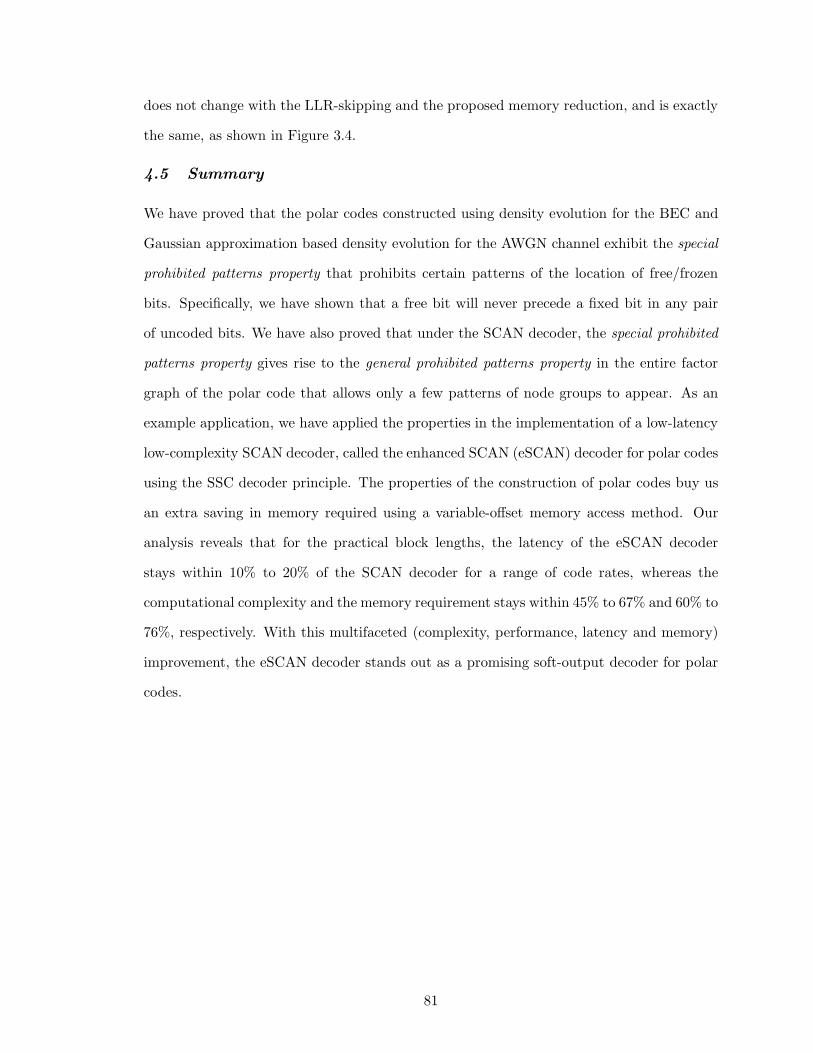
does not change with the LLR-skipping and the proposed memory reduction, and is exactly
the same, as shown in Figure 3.4.
4.5 Summary
We have proved that the polar codes constructed using density evolution for the BEC and
Gaussian approximation based density evolution for the AWGN channel exhibit the special
prohibited patterns property that prohibits certain patterns of the location of free/frozen
bits. Specifically, we have shown that a free bit will never precede a fixed bit in any pair
of uncoded bits. We have also proved that under the SCAN decoder, the special prohibited
patterns property gives rise to the general prohibited patterns property in the entire factor
graph of the polar code that allows only a few patterns of node groups to appear. As an
example application, we have applied the properties in the implementation of a low-latency
low-complexity SCAN decoder, called the enhanced SCAN (eSCAN) decoder for polar codes
using the SSC decoder principle. The properties of the construction of polar codes buy us
an extra saving in memory required using a variable-offset memory access method. Our
analysis reveals that for the practical block lengths, the latency of the eSCAN decoder
stays within 10% to 20% of the SCAN decoder for a range of code rates, whereas the
computational complexity and the memory requirement stays within 45% to 67% and 60% to
76%, respectively. With this multifaceted (complexity, performance, latency and memory)
improvement, the eSCAN decoder stands out as a promising soft-output decoder for polar
codes.
81

CHAPTER V
OPTIMIZED POLAR CODE DESIGN FOR INTERSYMBOL
INTERFERENCE CHANNELS
An effective strategy for error-control decoding over an intersymbol interference (ISI)
channel is turbo equalization [6], in which the cascade of the encoder and ISI channel
is viewed as a serial concatenation, and the receiver iteratively exchanges soft information
between the ISI detector and decoder. In Chapter 3 and 4, we designed the soft-output
decoder for polar codes that enabled polar codes in this turbo-based framework. In addition
to the soft-output decoder, a turbo-based system requires codes designed for the ISI channel.
While codes designed for the AWGN channel can perform adequately in this setting,
better performance can be achieved when the code is specifically tailored to match the
characteristics of the given ISI channel.
Code design for ISI channels has been limited to LDPC codes, and in this setting, three
different strategies for code design have emerged: density evolution is used in [28] and [29],
the extrinsic information transfer (EXIT) charts of ten Brink [30] are used in [31], and
multistage decoding of multilevel codes is used in [32]. Although there has been much work
regarding polar code design for the AWGN channel as well as soft-output decoders for polar
codes based on belief propagation [33] and SCAN [34], the problem of designing good polar
codes for ISI channels, to the best of our knowledge, remains unexplored in literature until
now.
This chapter proposes a solution to the problem of designing polar codes for ISI channels
with iterative decoding. We describe a design methodology to construct polar codes tailored
for an ISI channel and with performance close to LDPC codes. Specifically, we employ
the multilevel description of polar codes [1], analyze the shape of the EXIT curve under
multilevel decoding, and following [30] and [31] formulate the problem of code design as
one of matching the EXIT curve of the polar code with that of the ISI channel. We then
82

propose a graphical strategy to design the rates of different component polar codes in
the multilevel description to achieve the required curve matching. We present numerical
results demonstrating that the polar codes designed using our method outperform the codes
designed for the AWGN channel when used over an ISI channel. For example, for the EPR4
and E2PR4 channels we observe a gain of 0.6 dB and 0.9 dB, respectively, using our designs
when compared to polar codes designed for the AWGN channel.
The structure of the chapter is as follows. We introduce polar codes as generalized
concatenated codes as done by Trifonov and Semenov [1] and then give a primer on EXIT
charts. Then, we describe our EXIT curve analysis of polar codes in Section 5.3. Section
5.4 describes the design methodology based on the EXIT chart analysis, and in Section 5.5,
we present our conclusions.
5.1 Polar Codes as Generalized Concatenated Codes
Trifonov and Semenov [1] demonstrated that polar codes are a class of generalized
concatenated codes, and that successive cancellation decoding is an instance of multistage
decoding.
As a special case, we can view a parent polar code of length N as the concatenation
of two outer polar codes of length N/2 with an inner polar code of length N , as shown in
Figure 5.1. Similarly, we can decode this polar code of length N using a multistage decoder
in which we individually decode one of the polar codes of length N/2, use its output as
prior input to the inner decoder, and then decode the other polar code of length N/2.
Figure 5.1 shows an example concatenation of two length-four outer polar codes to a
rate-one inner code of length eight, constructing a parent polar code of length eight. To
decode this code, we can first use any decoder (the SC or any of its variants such as the
successive cancellation list decoder [5]) to decode the outer code C0. The inner decoder uses
extrinsic LLRs in B1(0, i)N/2i=0 to compute L1(1, i)N/2
i=0 , which is input to the decoder of
C1. After successful decoding of C1, the multistage decoder uses (3.5) and (3.6) at λ = 1 to
calculate B0(0, i)Ni=0 and completes the decoding of the parent code.
83
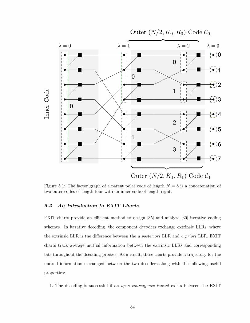
0
0
1
0
1
2
3
0
1
2
3
4
5
6
7
Figure 5.1: The factor graph of a parent polar code of length N = 8 is a concatenation oftwo outer codes of length four with an inner code of length eight.
5.2 An Introduction to EXIT Charts
EXIT charts provide an efficient method to design [35] and analyze [30] iterative coding
schemes. In iterative decoding, the component decoders exchange extrinsic LLRs, where
the extrinsic LLR is the difference between the a posteriori LLR and a priori LLR. EXIT
charts track average mutual information between the extrinsic LLRs and corresponding
bits throughout the decoding process. As a result, these charts provide a trajectory for the
mutual information exchanged between the two decoders along with the following useful
properties:
1. The decoding is successful if an open convergence tunnel exists between the EXIT
84
curves of the two decoders [30].
2. One can design efficient codes by matching the two curves of the component decoders
using curve-fitting techniques [35]. The better the matching is, the higher the code
rate is and the more iterations are required.
We follow the notation of [35] to describe the following different methods of computing the
EXIT curves:
1. Using Monte Carlo Simulations: This method applies to any decoder, specially for
which analytical methods do not exist such as the BCJR decoder. In this method, to
compute the EXIT curve of the BCJR decoder/equalizer for a channel of certain SNR,
we compute histogram of extrinsic LLRs corresponding to a large number of frames,
assuming that a Gaussian source generates a priori LLRs of mutual information IA.
This histogram gives us the extrinsic mutual information IE. Figure 5.2 explains this
method and the step-by-step procedure to calculate IE corresponding to a given IA
is as follows:
(a) A Priori LLRs LA Generation: Generate Gaussian-distributed LLRs by adding
σ2Axi/2 to a Gaussian source N (0, σ2A), where σA = J−1(IA), xi ∈ −1, 1 are
source symbols, and functions J(.) and J−1(.) are defined in [35, Appendix].
(b) Channel LLRs LC Generation: Pass source symbols x through the ISI channel
and the AWGN channel of zero mean and variance σ2N . The output of the AWGN
channel multiplied by 2/σ2N gives us channel LLRs LC .
(c) Extrinsic LLRs LE Generation: Given the channel observations in LC and
a priori information from LA, compute extrinsic LLRs LE using the BCJR
equalizer/decoder.
(d) Calculation of Extrinsic Information: Given LE , calculate histogram p(LE/xi =
85
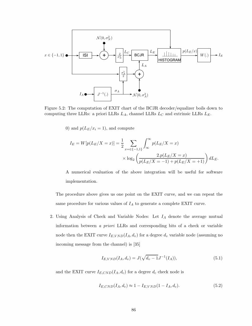
BCJR
HISTOGRAM
+
+ISI
Figure 5.2: The computation of EXIT chart of the BCJR decoder/equalizer boils down tocomputing three LLRs: a priori LLRs LA, channel LLRs LC and extrinsic LLRs LE .
0) and p(LE/xi = 1), and compute
IE =W [p(LE/X = x)] =1
2
∑
x=∈−1,1
∫ ∞
∞p(LE/X = x)
× log2
(2.p(LE/X = x)
p(LE/X = −1) + p(LE/X = +1)
)
dLE .
A numerical evaluation of the above integration will be useful for software
implementation.
The procedure above gives us one point on the EXIT curve, and we can repeat the
same procedure for various values of IA to generate a complete EXIT curve.
2. Using Analysis of Check and Variable Nodes: Let IA denote the average mutual
information between a priori LLRs and corresponding bits of a check or variable
node then the EXIT curve IE,V ND(IA, dv) for a degree dv variable node (assuming no
incoming message from the channel) is [35]
IE,V ND(IA, dv) = J(√
dv − 1J−1(IA)), (5.1)
and the EXIT curve IE,CND(IA, dc) for a degree dc check node is
IE,CND(IA, dc) ≈ 1− IE,V ND(1− IA, dc). (5.2)
86
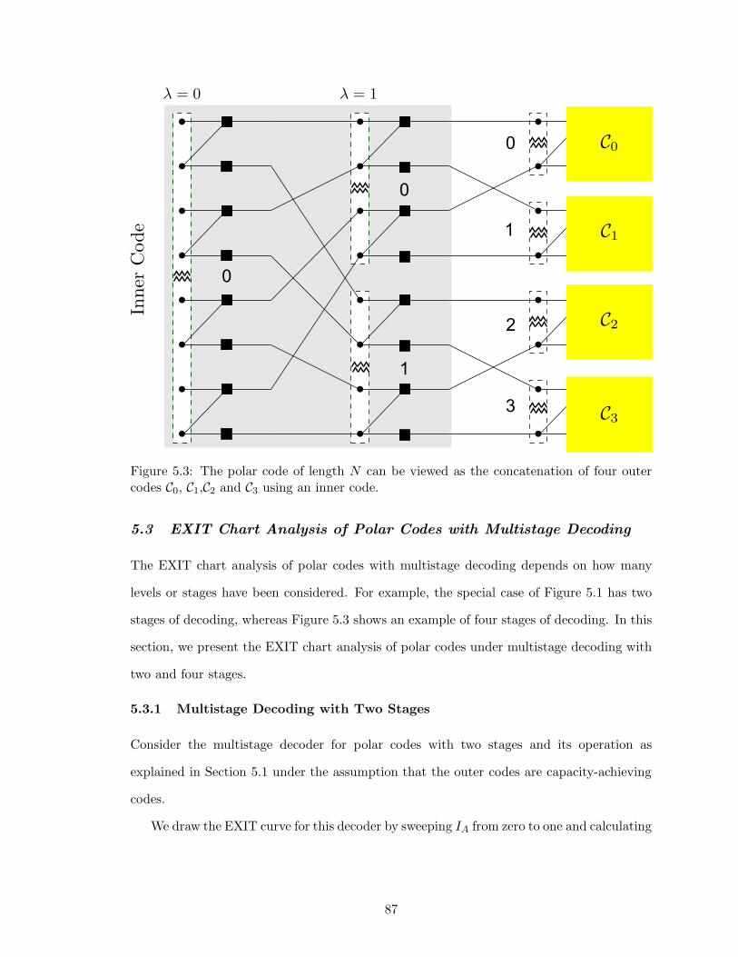
0
0
1
0
1
2
3
Figure 5.3: The polar code of length N can be viewed as the concatenation of four outercodes C0, C1,C2 and C3 using an inner code.
5.3 EXIT Chart Analysis of Polar Codes with Multistage Decoding
The EXIT chart analysis of polar codes with multistage decoding depends on how many
levels or stages have been considered. For example, the special case of Figure 5.1 has two
stages of decoding, whereas Figure 5.3 shows an example of four stages of decoding. In this
section, we present the EXIT chart analysis of polar codes under multistage decoding with
two and four stages.
5.3.1 Multistage Decoding with Two Stages
Consider the multistage decoder for polar codes with two stages and its operation as
explained in Section 5.1 under the assumption that the outer codes are capacity-achieving
codes.
We draw the EXIT curve for this decoder by sweeping IA from zero to one and calculating
87

IE , where
IA = I(L0(0, i)N−1i=0 ,v) and IE = I(B0(0, i)N−1
i=0 ,v).
Let IA,Ci and IE,Ci denote the input and output mutual information of the decoder for
outer code Ci. Let Ri denote the rate of the code Ci.
The following description of multilevel decoding applies directly if the component
decoders are SC or the SCL decoders. In the case of the SCAN decoder, the following
description applies to the last iteration of the decoder.
As we increase the values of IA, we observe the following different stages of this EXIT
curve in the inverted graph (IA versus IE):
1. Lower Face: This is the first part of the EXIT curve, as we increase IA from zero.
As described in Section 5.1, the multistage decoder first decodes C0, assuming no
information from the decoder of C1 and converts the inner code into a mixture of check
nodes of degree three, as shown in Figure 5.5. Since the EXIT curve of a code mixture
is average of the EXIT curves of the component codes [35], the mutual information
corresponding to a priori input to the decoder of C0 is IA,C0 = IE,CND(IA, 3). As we
have assumed that the outer code C0 is capacity-achieving, the decoder will remain
unsuccessful for as long as R0 ≥ IA,C0 . Alternatively,
IE = 0 for 0 ≤ IA ≤ I−1E,CND(R0, 3).
We call the region of IE = 0 the lower face.
2. Lower Plateau: As soon as IA > I−1E,CND(R0, 3), the decoder for outer code C0
successfully decodes the message u0, u1, . . . , uN/2−1, and therefore, the average
extrinsic mutual information at the output of the decoder for C0 is maximum, i.e.,
IE,C0 = 1. Thus, the perfect recovery of bits corresponding to B1(0, i)N/2−1i=0 converts
the inner code into a repetition code by removing the top right edge of all the
protographs in the inner code, as shown in Figure 5.5.
When the inner code is behaving as a repetition code, and the decoder for C1 is
unsuccessful, IE = IE,CND(IA, 2) = IA. The equality IE = IA can also be explained
88
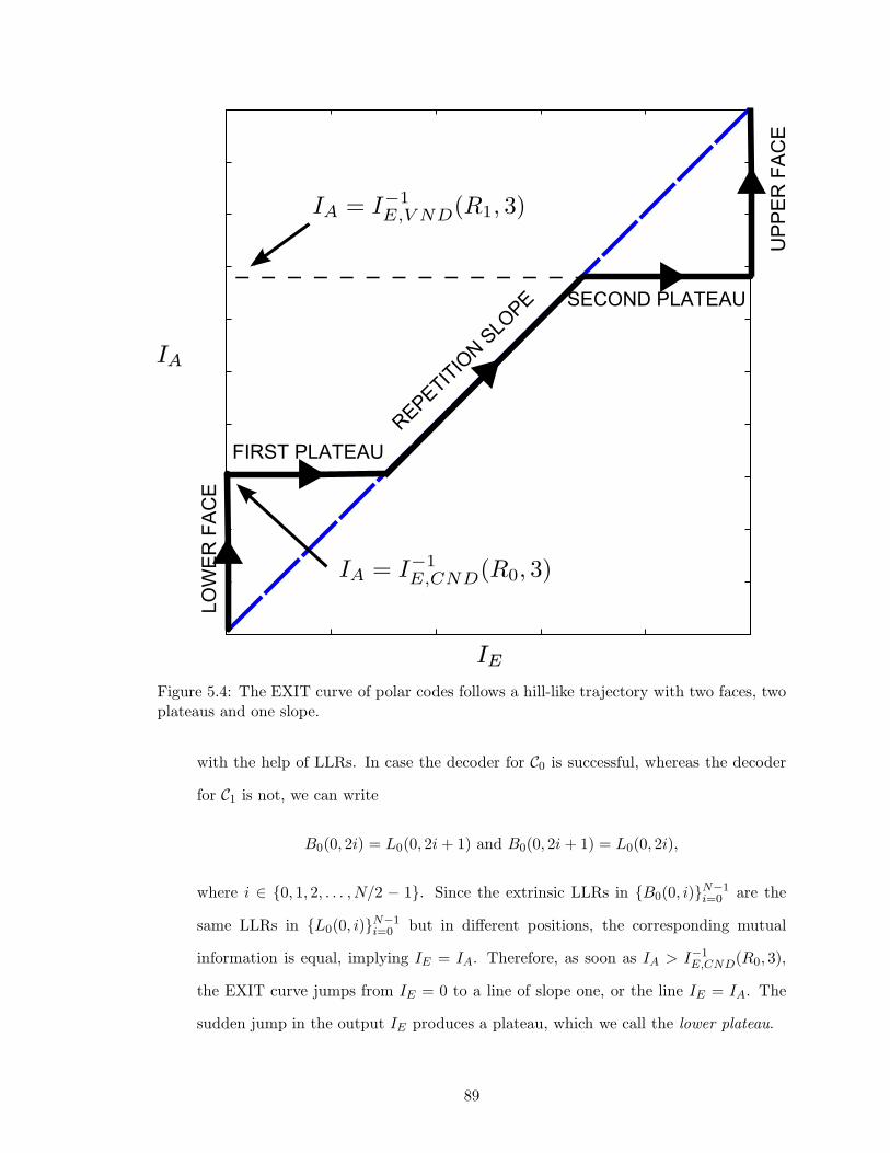
Figure 5.4: The EXIT curve of polar codes follows a hill-like trajectory with two faces, twoplateaus and one slope.
with the help of LLRs. In case the decoder for C0 is successful, whereas the decoder
for C1 is not, we can write
B0(0, 2i) = L0(0, 2i + 1) and B0(0, 2i + 1) = L0(0, 2i),
where i ∈ 0, 1, 2, . . . , N/2 − 1. Since the extrinsic LLRs in B0(0, i)N−1i=0 are the
same LLRs in L0(0, i)N−1i=0 but in different positions, the corresponding mutual
information is equal, implying IE = IA. Therefore, as soon as IA > I−1E,CND(R0, 3),
the EXIT curve jumps from IE = 0 to a line of slope one, or the line IE = IA. The
sudden jump in the output IE produces a plateau, which we call the lower plateau.
89
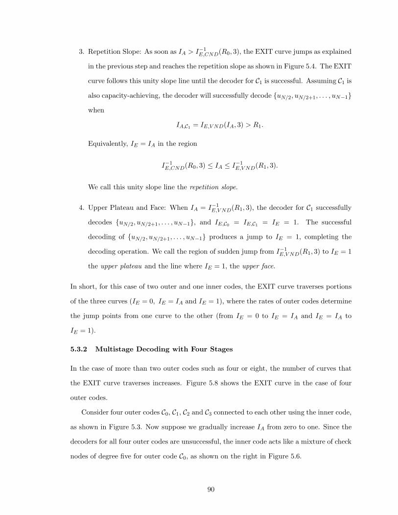
3. Repetition Slope: As soon as IA > I−1E,CND(R0, 3), the EXIT curve jumps as explained
in the previous step and reaches the repetition slope as shown in Figure 5.4. The EXIT
curve follows this unity slope line until the decoder for C1 is successful. Assuming C1 is
also capacity-achieving, the decoder will successfully decode uN/2, uN/2+1, . . . , uN−1
when
IA,C1 = IE,V ND(IA, 3) > R1.
Equivalently, IE = IA in the region
I−1E,CND(R0, 3) ≤ IA ≤ I−1
E,V ND(R1, 3).
We call this unity slope line the repetition slope.
4. Upper Plateau and Face: When IA = I−1E,V ND(R1, 3), the decoder for C1 successfully
decodes uN/2, uN/2+1, . . . , uN−1, and IE,C0 = IE,C1 = IE = 1. The successful
decoding of uN/2, uN/2+1, . . . , uN−1 produces a jump to IE = 1, completing the
decoding operation. We call the region of sudden jump from I−1E,V ND(R1, 3) to IE = 1
the upper plateau and the line where IE = 1, the upper face.
In short, for this case of two outer and one inner codes, the EXIT curve traverses portions
of the three curves (IE = 0, IE = IA and IE = 1), where the rates of outer codes determine
the jump points from one curve to the other (from IE = 0 to IE = IA and IE = IA to
IE = 1).
5.3.2 Multistage Decoding with Four Stages
In the case of more than two outer codes such as four or eight, the number of curves that
the EXIT curve traverses increases. Figure 5.8 shows the EXIT curve in the case of four
outer codes.
Consider four outer codes C0, C1, C2 and C3 connected to each other using the inner code,
as shown in Figure 5.3. Now suppose we gradually increase IA from zero to one. Since the
decoders for all four outer codes are unsuccessful, the inner code acts like a mixture of check
nodes of degree five for outer code C0, as shown on the right in Figure 5.6.
90
Figure 5.5: The inner code serves as the parity check and repetition code of degree threewhen the decoder for C1 is unsuccessful and the decoder for C0 is successful, respectively.
Consider the mixture of degree-five check nodes on the right in Figure 5.6. The extrinsic
mutual information of this code mixture, which is also the input mutual information for
the decoder of C0, is IA,C0 = IE,CND(IA, 5). Since C0 is unsuccessful, the extrinsic mutual
information IE,C0 from the decoder for C0 is zero. As a result of unsuccessful decoding by
all the outer decoders, the extrinsic mutual information IE of the multistage decoder is also
zero.
As we have assumed that the outer code C0 is capacity-achieving, the decoder for C0 will
remain unsuccessful for as long as R0 ≥ IA,C0 . Alternatively,
IE = 0 for 0 ≤ IA ≤ I−1E,CND(R0, 5).
As soon as IA > I−1E,CND(R0, 5), the decoder for C0 is successful. When the decoder
for C0 is successful, the inner code becomes the concatenation of degree-three check and
91

...
...
...
Mixture of Degree-5
Check Nodes
Figure 5.6: When decoders for outer codes C0, C1, C2 and C3 are unsuccessful, the innercode acts like a mixture of degree-five parity-check codes. The extrinsic mutual informationat the output of the multistage decoder is zero, because all the decoders for C0, C1, C2 andC3 are unable to decode the message.
Figure 5.7: When the decoders for outer code C0 and C1 are successful and unsuccessful,respectively, the inner code becomes a code mixture of serially concatenated degree-threeparity-check and degree-three variable nodes.
and degree-three variable nodes, as shown on the right of Figure 5.7. The extrinsic mutual
information of this concatenated code, which is also the input mutual information for the
decoder of code C1, is IE,VND(IE,CND(IA, 3), 3). Since the decoder for C1 is unsuccessful,
IE,C1 = 0, which essentially removes the edges connecting C1 and inner code. As a result,
the extrinsic mutual information IE of the multistage decoder is the extrinsic mutual
information of a mixture of degree-four parity-check codes IE,CND(IA, 4).
The EXIT curve stays on the curve IE = IE,CND(IA, 4) until the decoder for C1
92

succeeds when the input mutual information IA,C1 = IE,V ND(IE,CND(IA, 3), 3) > R1. At
this point, the EXIT curve jumps to IE = IA in a similar way to the lower plateau in
Section 5.3.1. The EXIT curve traverses IE = IA until the decoder for C2 succeeds at
IA,C2 = IE,CND(IE,V ND(IA, 3), 3). Equivalently, the EXIT curve stays on IE = IA line for
as long as
I−1E,CND(I
−1E,V ND(R1, 3), 3) ≤ IA ≤ I−1
E,V ND(I−1E,CND(R2, 3), 3).
When IA > I−1E,VND(I
−1E,CND(R2, 3), 3), the decoder for C3 succeeds, and the EXIT curve
jumps to IE = IE,VND(IA, 4).
The EXIT curve follows IE = IE,VND(IA, 4) until the decoder for C3 succeeds when
IA,C3 = IE,V ND(IA, 5) > R3 with a jump to IE = 1 curve. At this point, the decoding of
the message u is complete.
5.4 EXIT Chart Based Design of Polar Codes
Figure 5.9 shows the EXIT curve for the BCJR equalizer in the dicode, the EPR4 and the
E2PR4 channels, defined by the impulse response
h =
[
1 −1]
/√2,
h =
[
1 1 −1 −1]
/2,
h =
[
1 2 0 −2 −1]
/√10,
respectively. It is evident that with the increasing intersymbol interference, the EXIT curves
of the channels become steeper, and for better performance under iterative decoding, the
EXIT curve of the code needs to match to these steep curves as closely as possible.
As explained in Section 5.3, by changing the rates of the component codes in the
multistage description of polar codes, we can produce the jump points giving the EXIT
curve a sloped shape. The sloped EXIT curve provides better matching to the EXIT curve
of the ISI channel, which facilitates an open convergence tunnel between the two curves.
This open tunnel allows the iterative decoder to follow a trajectory that ends at IE = 1
or equivalently successful decoding. Based on this observation, we propose the following
design method for polar codes of rate R for ISI channels.
93

0 10
1
Figure 5.8: The EXIT curve of polar codes follows a hill-like trajectory for four-level codes.
5.4.1 For Decoding with Two Stages
1. Fix the search space size as M codes. Draw the EXIT curve of the ISI channel for
(Eb/N0)R × (1 + ∆), where ∆ > 0 is arbitrarily small, and (Eb/N0)R denotes the
Eb/N0 required by a capacity-achieving modulation scheme to transmit on an ISI
channel with rate R and an independent, uniformly distributed (IUD) binary source.
One simulation-based technique to compute (Eb/N0)R is discussed in [36]. Let (0, a)
be the intersection point of this curve with y-axis (IE = 0).
2. Draw a unity slope line connecting the points (0, 0) and (1, 1). Let (b, b) be the
94

intersection point of the unity slope line with the line of step 1.
3. If
R+M/N > (IE,CND(a, 3) + IE,V ND(b, 3))/2,
go to step 1 and repeat with increased ∆, else proceed to step 4.
4. Perform a search in the following region for the code with best frame error rate (FER):
R0 < IE,CND(a, 3),
R1 < IE,VND(b, 3),
R =
(R0 +R1
2
)
.
5.4.2 For Decoding with Four Stages
1. Fix the search space size as M codes. Draw the EXIT curve of the ISI channel for
(Eb/N0)R × (1 + ∆), where ∆ > 0 is arbitrarily small, and (Eb/N0)R denotes the
Eb/N0 required by a capacity-achieving modulation scheme to transmit on an ISI
channel with rate R and an independent, uniformly distributed (IUD) binary source.
One simulation-based technique to compute (Eb/N0)R is discussed in [36]. Let the
curve be IE = IE,CH(IA)
2. Let (0, y0), (·, y1), (·, y2) and (·, y3) be the intersection points of this curve with the
lines IE = 0, IA = I−1E,CND(IE , 4), IA = IE and IA = I−1
E,VND(IE , 4), respectively and
ρ0 = IE,CND(y0, 5) (5.3)
ρ1 = IE,CND(IE,V ND(y1, 3), 3) (5.4)
ρ2 = IE,V ND(IE,CND(y2, 3), 3) (5.5)
ρ3 = IE,V ND(y3, 5) (5.6)
3. If
R+M/N >3∑
i=0
ρi,
repeat from step 1 with an increased ∆, else proceed to step 4.
95

4. Perform a search in the following region for the code with best frame error rate (FER):
1− (ρ0 + ρ1) < R1 < ρ2 + ρ3.
5.4.3 Computation of Design SNR
The second design parameter is the SNR to which the component polar codes will be
optimized. One empirically good design strategy we found is to design component polar
codes optimized to the design SNR γ0 and γ1 given by
γ0 =h−1
(
1− [1− h(2γ)]2)
2and γ1 = 2γ, (5.7)
where
h(x) =
e−0.4527x0.86+0.0218 x > 10,
√πxe
−x4
[1− 10
7x
]otherwise.
(5.8)
γ0 and γ1 represent the SNRs corresponding to the LLRs in L1(0, i)N/2i=0 and L1(1, i)N/2
i=0 ,
respectively calculated using the density evolution (DE) based on Gaussian assumption [1].
The DE procedure assumes that the SNR γ corresponding to the LLRs in L0(0, i)Ni=0 is
given by
γ = (Eb/N0)R ×∆Eb(N)× 2R, (5.9)
where ∆Eb(N) is excess energy per bit over the energy per bit required to achieve capacity
for a block length N . γ is a crude guess about the SNR required to achieve rate-R
communication over the ISI channel at a finite block length N . We refer the interested
reader to [37] for the computation of ∆Eb(N) and will just state the quantity wherever
needed.
Example 5.1 (EPR4 Channel). Suppose we want to design a polar code of length 8192
with R = 1/2 for the EPR4 channel. For this example, we apply the design method for
the two-level description of polar codes. We first fix the search space size to M = 50 codes.
Using the method in Section 5.2, we draw EXIT curve for the EPR4 channel using the BCJR
equalizer for (Eb/N0)1/2 = 1.16 dB which is the minimum Eb/N0 required for rate-0.5 (to
96

be precise 0.5012) transmission [36]. A linear approximation to this EXIT curve generates
IE = 0.16IA + 0.44. (5.10)
Solving (5.10) and IE = IA results in b = 0.5238. Since
(IE,CND(a, 3) + IE,V ND(b, 3)
2
)
= 0.4929 < 0.5 + 0.0061,
we cannot achieve rate-0.5 transmission with the rate pair (R0, R1), where R0 =
IE,CND(a, 3) and R1 = IE,V ND(b, 3). We go back to step 1 and repeat with increased ∆.
After a few iterations, we reach the EXIT curve for the EPR4 channel with Eb/N0 = 1.8
dB. This curve has the following linear approximation:
IE = 0.17IA + 0.46, (5.11)
with a = 0.46. Solving (5.11) and IE = IA results in b = 0.5542. Since
(IE,CND(a, 3) + IE,V ND(b, 3)
2
)
= 0.5067 > 0.5 + 0.0061,
according to step 3, the design is possible. The code search region is as follows:
R0 < 0.2267, R1 < 0.7867,
(R0 +R1
2
)
= 0.5,
that simplifies to
1−R0 < R1 < 0.7867 =⇒ 0.7733 < R1 < 0.7867
in terms of rates and
3167 < K1 < 3222,
in terms of dimensions of component codes of length 4096, respectively. For the design SNR
of different component codes, we know the following parameters for the EPR4 channel:
(Eb/N0)1/2 = 1.16 dB , ∆Eb(8192) ≈ 0.4 dB ,
where ∆Eb is calculated to achieve an error rate of 10−5. Using these parameters in (5.9),
we calculate SNR γ = 1.6 dB (after rounding off). This γ along with (5.7) gives γ0 =
−1.45 dB and γ1 = 4.6 dB .
97
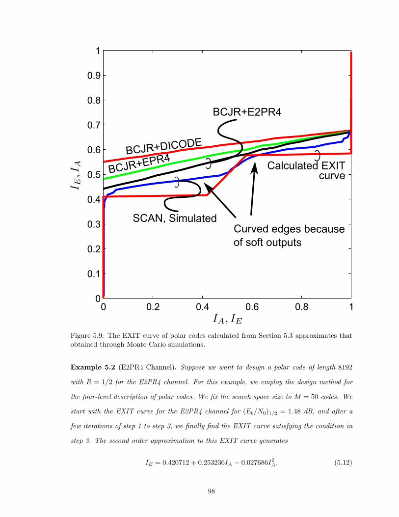
Figure 5.9: The EXIT curve of polar codes calculated from Section 5.3 approximates thatobtained through Monte Carlo simulations.
Example 5.2 (E2PR4 Channel). Suppose we want to design a polar code of length 8192
with R = 1/2 for the E2PR4 channel. For this example, we employ the design method for
the four-level description of polar codes. We fix the search space size to M = 50 codes. We
start with the EXIT curve for the E2PR4 channel for (Eb/N0)1/2 = 1.48 dB, and after a
few iterations of step 1 to step 3, we finally find the EXIT curve satisfying the condition in
step 3. The second order approximation to this EXIT curve generates
IE = 0.420712 + 0.253236IA − 0.027686I2A. (5.12)
98

Using (5.12) in step 3 results in
y0 = 0.420712, y1 = 0.447026, y2 = 0.552080, y3 = 0.999751,
ρ0 = 0.041606, ρ1 = 0.375103, ρ2 = 0.623617, ρ3 = 1.000000.
Since
1
4
3∑
i=0
ρi = 0.510082 > 0.500000 + 0.006104,
according to step 3, the design is possible. The code search region is as follows:
R0 < (ρ0 + ρ1)/2, R1 < (ρ2 + ρ3)/2,(R0 +R1
2
)
= 0.5,
that simplifies to
1−R0 < R1 < 0.811809 =⇒ 0.791645 < R1 < 0.811809
in terms of rates and
3243 < K1 < 3326,
in terms of dimensions of component polar codes of length 4096, respectively. For design
SNR, following the similar approach to the previous example, we get the following:
(Eb/N0)1/2 = 1.48 dB , ∆Eb(8192) ≈ 0.4 dB ,
γ = 1.9 dB , γ0 = −1.0189 dB , γ1 = 4.9 dB .
5.5 Simulation Results
In this section, we show that the EXIT curve of polar codes with the SCAN decoder follows
the approximation presented in Section 5.3. We further compare the error-rate performance
of the polar codes designed using our proposed method with the polar codes designed for the
AWGN channel when decoded using the SCAN decoder in turbo equalization framework.
99

Table 3: Design Parameters
Channel Code N K Design SNR
EPR4
C0 4096 894 -1.45 dB
C1 4096 3202 4.6 dB
Classical 8192 4096 1.4 dB
E2PR4
C0 4096 770 -1.01 dB
C1 4096 3326 4.9 dB
Classical 8192 4096 1.6 dB
5.5.1 Accuracy of EXIT Curve Approximation
We have calculated the EXIT curve of the SCAN decoder for the polar code in Example
5.2 using Monte Carlo simulations, as explained in Section 5.3. The jump points in the
simulated curve closely follow the predicted jump points in the EXIT curve calculated
using the analysis in Section 5.3.
We also observe smooth edges in the EXIT curve for the SCAN decoder on the two
jump points (at the start of both the plateaus) rather than the sudden transitions in the
calculated EXIT curve. This smoothness is because we assumed in Section 5.3 that the
outer decoders are capacity-achieving and hard-output, i.e., either they deliver complete
information with IE = 1 or no information IE = 0, but not in between. On the other
hand, the SCAN decoder is a soft-output decoder that provides a smooth transition instead
of a sudden jump. This smooth transition reduces the area between the EXIT curve of
the SCAN decoder and that of the ISI channel relative to the calculated EXIT curve and
directly corresponds to the reduction in the rate loss (C −R) [38], where C is the capacity
of the channel for IUD binary source.
5.5.2 Code Performance
We have simulated polar codes designed in Example 5.1 and 5.2 and compared them with
classical polar codes. We have designed the classical as well as both the component polar
codes in the two examples using the method of [1]. For classical polar codes, we swept the
design SNR from 1 dB to 3 dB with a step of 0.1 dB and picked the one that resulted in
100

Figure 5.10: Polar codes constructed through the proposed method provide approximately0.6 dB and 0.9 dB gain in FER performance on EPR4 and E2PR4 channels, respectively,relative to the ones optimized for AWGN.
the best FER performance at a certain Eb/N0. For all polar code simulations, a maximum
of six turbo iterations and eight SCAN iterations are used.
In the code search space in both of the examples, we observed that the majority of the
codes perform well with negligible difference in error rate from each other. Therefore, the
search for M = 50 codes in both of the examples suffices to reach a code that performs
either equal or closer to the best code in the entire code search space. Table 3 summarizes
different polar codes used in Figure 5.10. We observed a gain of 0.6 dB and 0.9 dB in the
proposed design of polar codes as compared to the classical designs for FER = 10−4.
We also compared the proposed polar codes to an irregular LDPC code of the variable
node distribution λ(x) = 0.2184x+ 0.163x2 + 0.6186x3 and check node distribution ρ(x) =
0.6821x4 + 0.3173x5 + 0.0006x6 designed using progressive edge growth (PEG) method
101

[23], [21], [22]. For LDPC simulations, we have used a maximum of six turbo and 40 BP
iterations. We observed that polar codes for both EPR4 and E2PR4 channels perform
approximately 0.25 dB and 0.2 dB away from respective LDPC codes.
In fairness, we mention here that the simulated LDPC code is optimized for the AWGN
channel with lower values of maximum variable and check node degrees and LDPC codes
optimized for ISI channels exist such as reported in [28]. But, the caveat, however, is that
such optimal LDPC codes usually have very higher maximum variable node and check node
degrees that make these codes difficult to realize in hardware.
5.6 Summary
In this chapter, we presented a method to design polar codes for intersymbol interference
channels. The proposed method utilizes the multilevel description of polar codes and
optimizes the rates of component codes for ISI channels under iterative decoding. We showed
that by changing the rates of the component polar codes, we can match the EXIT curve
of a polar code to that of a ISI channel. We also provided numerical results demonstrating
significant gains relative to codes designed for the AWGN channel. Specifically, we observed
a gain of 0.6 dB and 0.9 dB in the proposed designs for EPR4 and E2PR4 channels,
respectively, relative to the classical design of polar codes for the AWGN channel.
102
CHAPTER VI
CONTRIBUTIONS AND FUTURE RESEARCH
This thesis presents polar codes as a strong candidate for magnetic recording application.
In current state, polar codes have neither the optimized designs nor near-optimal,
low-complexity, soft-output decoders for magnetic recording channels. This thesis provides
an error-correcting system based on optimized polar codes for magnetic recording channels
and a low-complexity, high-throughput soft-output decoder for polar codes. In this chapter,
we summarize all the contributions of this thesis and then discuss a few directions in which
this work can be extended.
6.1 Contributions
Following are the main contributions of this thesis:
1. In Chapter 3, we proposed a low-complexity soft-output decoder called the
soft-cancellation (SCAN) decoder. We demonstrated that the serial schedule of
message updates in the SCAN decoder converges much faster than the flooding
schedule of previous BP decoder, resulting in drastically reduced computational
complexity. The low complexity of SCAN combined with other properties of polar
codes such as universal rate adaptability, puts polar codes in a strong position with
other competing code families in magnetic recording application. The complexity
reduction does not compromise error-rate performance at all, and the SCAN decoder
outperforms the SC and the BP decoders in both the AWGN and the ISI channels.
2. In Chapter 4, we demonstrated that polar codes exhibit special prohibited pair property
according to which only a few of all the possible patterns in the location of frozen bits
are possible. Specifically, if we pair two consecutive bits in the successive-cancellation
detection order, a free bit will never precede a fixed bit. We also showed that
this property generalizes to the general prohibited pair property under SCAN in the
103
sense that a few of all the possible patterns of node groups are possible. Both of
the properties describe the type of LLRs in the entire factor graphs based on the
location of fixed bits. We apply these properties to the SCAN decoder and propose
a high-throughput and memory-efficient implementation of the SCAN decoder called
the enhanced SCAN (eSCAN) decoder.
3. In Chapter 5, we proposed a method to design polar codes for ISI channels when the
SCAN decoder is used. The method is based on the well-known result that under
turbo equalization, EXIT curves of optimal codes match those of ISI channels. This
result reduces the problem of finding better codes into a curve-fitting problem in which
we try to fit the EXIT curve of the code to that of the ISI channel. The better this
matching is, the better the codes perform in terms of error rates. We demonstrated
that polar codes can have a sloped EXIT curve matched to that of an ISI channel,
outperforming the codes designed for the AWGN channel under turbo equalization.
We also provide a method to achieve this matching for a given channel. The polar
codes designed using the proposed method buy us a gain of 0.6 dB and 0.9 dB for
EPR4 and E2PR4 channels, respectively compared to the the codes designed for the
AWGN channel.
6.2 Future Directions
In the previous section, we outlined the main contributions of this thesis. This section
discusses a few directions in which our work can be extended.
6.2.1 Error Floor Analysis of Polar Codes with the SCAN Decoder
Error-rate curves for the iterative decoding usually exhibit two main regions as we increase
the SNR from a lower value to a higher one; namely, the waterfall region and the error-floor
region [39]. As we increase the SNR from a lower value, the error rate stays at some lower
value as well until it reaches a certain value of SNR. After this SNR, the error rate decreases
rapidly. This region of rapid error-rate drop is called the waterfall region. As we increase
the SNR even further, it is observed that the error rate stops to decrease as rapidly as it
104

does in the waterfall region. This region of slow error-rate drop is called the error-floor
region.
All the performance curves in this thesis concern only the waterfall region as they
are easy to simulate using computer software. The waterfall region broadly defines the
performance of a coded system in most cases, however, some applications such as magnetic
recording and optical communication channels have stringent error-floor requirements. To
assess the performance of polar codes with the SCAN decoder in the error-floor region, we
need high-speed hardware platforms that can reach such low error rates. This necessitates
the research for hardware implementations of the SCAN decoder.
6.2.2 Analysis of the SCAN Decoder
All codes of rate R require a minimum block length N to achieve a certain frame-error
probability Pe. Although a single relationship between these three parameters is of immense
practical significance, it is usually very hard to find. Therefore, a relatively easier approach
is to reduce the size of the problem by fixing one of these three parameters and look at the
relationship between the remaining two variables. This reduction results in the following
two important cases:
1. Error Exponent: If we fix rate R and study the relationship between the
error-probability Pe and block length N , we end up with the concept of an error
exponent. Precisely, if the error probability of a code decays as Pe = e−Nα, then α is
called the error exponent.
For instance, Arikan and Telatar [40] showed that under the SC decoder polar codes
attain an exponent of 1/2. In other words, for any β < 1/2 and R < C, where R is
the rate of the code and C is the capacity of the channel, the block-error probability is
upper bounded by 2−Nβ
. This rapid exponential decay of error probability guarantees
an error-rate curve with no error floor for moderate to large block lengths. For the
SCAN decoder, no such guarantees exist; although, it outperforms the SC decoder in
error-rate performance in the AWGN channel. Therefore, one possible extension of
our work is to study the error exponent of polar codes under the SCAN decoding to
105
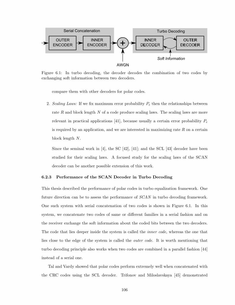
Serial Concatenation
+ C C
Soft Information
AWGN
Turbo Decoding
INNER
ENCODER
OUTER
ENCODER
Figure 6.1: In turbo decoding, the decoder decodes the combination of two codes byexchanging soft information between two decoders.
compare them with other decoders for polar codes.
2. Scaling Laws: If we fix maximum error probability Pe then the relationships between
rate R and block length N of a code produce scaling laws. The scaling laws are more
relevant in practical applications [41], because usually a certain error probability Pe
is required by an application, and we are interested in maximizing rate R on a certain
block length N .
Since the seminal work in [4], the SC [42], [41]; and the SCL [43] decoder have been
studied for their scaling laws. A focused study for the scaling laws of the SCAN
decoder can be another possible extension of this work.
6.2.3 Performance of the SCAN Decoder in Turbo Decoding
This thesis described the performance of polar codes in turbo equalization framework. One
future direction can be to assess the performance of SCAN in turbo decoding framework.
One such system with serial concatenation of two codes is shown in Figure 6.1. In this
system, we concatenate two codes of same or different families in a serial fashion and on
the receiver exchange the soft information about the coded bits between the two decoders.
The code that lies deeper inside the system is called the inner code, whereas the one that
lies close to the edge of the system is called the outer code. It is worth mentioning that
turbo decoding principle also works when two codes are combined in a parallel fashion [44]
instead of a serial one.
Tal and Vardy showed that polar codes perform extremely well when concatenated with
the CRC codes using the SCL decoder. Trifonov and Miloslavskaya [45] demonstrated
106
similar improvement in the performance of polar codes when concatenated with a
short-length parity-check code and decoded with a SCL decoder. Both of these codes
are examples of serially concatenated codes and can be decoded using the turbo decoding
framework. Our initial investigations show that the first CRC-concatenated code is hard
to decode this way, because no low-complexity soft-output decoder is available for them at
moderate to long block lengths. For short-length parity-check codes, the BP decoder for
LDPC codes do not work because of the relatively high-density of the code. In this context,
the following two important questions demand further exploration:
1. Is there a way to decode these concatenated codes using the SCAN decoder?
2. Which of these codes perform better under SCAN in turbo decoding framework?
107
APPENDIX A
PROOF OF THE PROPERTIES OF THE SCAN DECODER
Proof of Lemma 3.1.
W−(y0, y1, z1|u0)
=∑
u1
W2(y0, y1, z1, u1|u0)
=1
2
∑
u1
W (y0|u0 ⊕ u1)W (y1|u1)P (z1|u1). (A.1)
W+(y0, y1, z0|u1)
=∑
u0
W2(y0, y1, z0, u0|u1)
=1
2W (y1|u1)
∑
u0
W (y0|u0 ⊕ u1)P (z0|u0), (A.2)
where we have used the fact that both the bits u0, u1 are equally likely to be 0 or 1. Using
(A.1) and (A.2) with the definition of an LLR, we get (3.1) and (3.2).
Proof of Proposition 3.1. Consider the problem setup for (A.1) and (A.2). Recall for an SC
decoder, we have from [18]
Z(W+SC) = Z(W )2,
Z(W )√
2− Z(W )2 ≤ Z(W−SC) ≤ 2Z(W )− Z(W )2,
where Z(W ) is Bhattacharrya parameter of the DMC W defined as
Z(W ) ,∑
y
√
W (y|0)W (y|1). (A.3)
Since for the SCAN decoder with I = 1, the computation for the check-node doesn’t change,
the relationships for Z(W−) as described above hold. Therefore, we only need to prove
108

Z(W+) ≥ Z(W )2.
(A.4)
Z(W+) =∑
y0,y1,z0
√
W+(y0, y1, z0|0)W+(y0, y1, z0|1)
=1
2Z(W )×A(W,P ),
where
A(W,P ) =∑
y0,z0
(∑
u0
W (y0|u0)P (z0|u0))
×
∑
u′
0
W (y0|u′
0 ⊕ 1)P (z0|u′
0)
.
From Lemma 3.15 in [18], we have
(A.5)A(W,P ) ≥ 2√
Z(W )2 + Z(P )2 − Z(W )2Z(P )2.
Using (A.5) in (A.4), we get
Z(W+) = Z(W )2
√
1 + Z(P )2(
1
Z(W )2− 1
)
,
≥ Z(W )2
as by definition 0 ≤ Z(P ), Z(W ) ≤ 1.
109

REFERENCES
[1] P. Trifonov and P. Semenov, “Generalized concatenated codes based on polar codes,”in Proc. 8th Int. Symp. Wireless Commun. Syst., Nov. 2011, pp. 442–446.
[2] R. Galbraith and T. Oenning. (2008) Iterative detection readchannel technology in hard disk drives. [Online]. Available:http://www.hgst.com/tech/techlib.nsf/techdocs/FB376A33027F5A5F86257509001463AE/$file/IDRC˙WP˙final.pdf
[3] A. Jimenez Felstrom and K. Zigangirov, “Time-varying periodic convolutional codeswith low-density parity-check matrix,” IEEE Trans. Inf. Theory, vol. 45, no. 6, pp.2181–2191, Sep. 1999.
[4] E. Arikan, “Channel polarization: A method for constructing capacity-achieving codesfor symmetric binary-input memoryless channels,” IEEE Trans. Inf. Theory, vol. 55,no. 7, pp. 3051–3073, Jul. 2009.
[5] I. Tal and A. Vardy, “List decoding of polar codes,” in Proc. IEEE Int. Symp. Inform.Theory, Aug. 2011, pp. 1–5.
[6] C. Douillard, M. Jzquel, C. Berrou, D. Electronique, A. Picart, P. Didier, andA. Glavieux, “Iterative correction of intersymbol interference: Turbo-equalization,”European Trans. on Telecommun., vol. 6, no. 5, pp. 507–511, 1995.
[7] M. Mansour and N. Shanbhag, “High-throughput LDPC decoders,” IEEE Trans. VLSISyst., vol. 11, no. 6, pp. 976–996, Dec. 2003.
[8] C. Leroux, I. Tal, A. Vardy, and W. Gross, “Hardware architectures for successivecancellation decoding of polar codes,” in Proc. IEEE Int. Conf. Acoust., Speech andSignal Process., 2011, pp. 1665–1668.
[9] M. Mansour and N. Shanbhag, “A 640-mb/s 2048-bit programmable ldpc decoderchip,” IEEE J. Solid-State Circuits, vol. 41, no. 3, pp. 684–698, Mar. 2006.
[10] T. Richardson, M. Shokrollahi, and R. Urbanke, “Design of capacity-approachingirregular low-density parity-check codes,” IEEE Trans. Inf. Theory, vol. 47, no. 2,pp. 619–637, Feb. 2001.
[11] A. Alamdar-Yazdi and F. Kschischang, “A simplified successive-cancellation decoderfor polar codes,” IEEE Commun. Lett., vol. 15, no. 12, pp. 1378–1380, Dec. 2011.
[12] E. Arikan, “A survey of reed-muller codes from polar coding perspective,” inInformation Theory Workshop (ITW), 2010 IEEE, Jan 2010, pp. 1–5.
[13] F. Kschischang, B. Frey, and H.-A. Loeliger, “Factor graphs and the sum-productalgorithm,” IEEE Trans. Inf. Theory, vol. 47, no. 2, pp. 498–519, 2001.
110

[14] R. Mori and T. Tanaka, “Performance of polar codes with the construction usingdensity evolution,” IEEE Commun. Lett., vol. 13, no. 7, pp. 519–521, Jul. 2009.
[15] I. Tal and A. Vardy, “How to construct polar codes,” IEEE Trans. Inf. Theory, vol. 59,no. 10, pp. 6562–6582, Oct. 2013.
[16] L. Bahl, J. Cocke, F. Jelinek, and J. Raviv, “Optimal decoding of linear codes forminimizing symbol error rate,” IEEE Trans. Inf. Theory, vol. 20, no. 2, pp. 284–287,Mar. 1974.
[17] E. Arikan, “A performance comparison of polar codes and Reed-Muller codes,” IEEECommun. Lett., vol. 12, no. 6, pp. 447 –449, Jun. 2008.
[18] S. B. Korada, “Polar codes for channel and source coding,” Ph.D. dissertation, EPFL,Lausanne, 2009. [Online]. Available: http://library.epfl.ch/theses/?nr=4461
[19] H. Sankar and K. Narayanan, “Memory-efficient sum-product decoding of ldpc codes,”IEEE Trans. Commun., vol. 52, no. 8, pp. 1225–1230, Aug 2004.
[20] E. Zimmermann and G. Fettweis, “Reduced complexity LDPC decoding using forcedconvergence,” in Proc. 7th Int. Symp. Wireless Personal Multimedia Communications,2004, p. 15.
[21] X.-Y. Hu. Source code for Progressive Edge Growth parity-check matrix construction.[Online]. Available: http://www.cs.toronto.edu/ mackay/PEG˙ECC.html
[22] X.-Y. Hu, E. Eleftheriou, and D.-M. Arnold, “Progressive edge-growth tanner graphs,”in Proc. IEEE Global Commun. Conf., vol. 2, 2001, pp. 995–1001.
[23] LOPT - online optimisation of LDPC and RA degree distributions. [Online]. Available:http://sonic.newcastle.edu.au/ldpc/lopt/
[24] B. Li, H. Shen, and D. Tse, “An adaptive successive cancellation list decoder for polarcodes with cyclic redundancy check,” IEEE Commun. Lett., vol. 16, no. 12, pp. 2044–2047, Dec. 2012.
[25] S. Jeon and B. Kumar, “Performance and complexity of 32 k-bit binary LDPC codesfor magnetic recording channels,” IEEE Trans. Magn., vol. 46, no. 6, pp. 2244–2247,2010.
[26] J. Forney, G.D., “Codes on graphs: normal realizations,” IEEE Trans. Inf. Theory,vol. 47, no. 2, pp. 520–548, 2001.
[27] U. U. Fayyaz and J. Barry, “A Low-Complexity Soft-Output decoder for polar codes,”in Proc. IEEE Global Commun. Conf., Atlanta, USA, Dec. 2013.
[28] N. Varnica and A. Kavcic, “Optimized low-density parity-check codes for partialresponse channels,” IEEE Commun. Lett., vol. 7, no. 4, pp. 168–170, April 2003.
[29] A. Kavcic, X. Ma, and M. Mitzenmacher, “Binary intersymbol interference channels:Gallager codes, density evolution, and code performance bounds,” IEEE Trans. Inf.Theory, vol. 49, no. 7, pp. 1636–1652, July 2003.
111

[30] S. Ten Brink, “Convergence behavior of iteratively decoded parallel concatenatedcodes,” IEEE Trans. Commun., vol. 49, no. 10, pp. 1727–1737, Oct 2001.
[31] M. Franceschini, G. Ferrari, and R. Raheli, “Exit chart-based design of LDPC codes forinter-symbol interference channels,” in Proc. IST Mobile and Wireless CommunicationsSummit, 2005.
[32] J. B. Soriaga, H. Pfister, and P. Siegel, “Determining and approaching achievable ratesof binary intersymbol interference channels using multistage decoding,” IEEE Trans.Inf. Theory, vol. 53, no. 4, pp. 1416–1429, April 2007.
[33] N. Hussami, S. Korada, and R. Urbanke, “Performance of polar codes for channel andsource coding,” in Proc. IEEE Int. Symp. Inform. Theory, 2009, pp. 1488–1492.
[34] U. U. Fayyaz and J. R. Barry, “Low-complexity soft-output decoding of polar codes,”IEEE J. Sel. Areas Commun., vol. 32, no. 5, pp. 958–966, May 2014.
[35] S. ten Brink, G. Kramer, and A. Ashikhmin, “Design of low-density parity-check codesfor modulation and detection,” IEEE Trans. Commun., vol. 52, no. 4, pp. 670–678,Apr. 2004.
[36] D. Arnold and H.-A. Loeliger, “On the information rate of binary-input channels withmemory,” in Proc. IEEE Int. Conf. Commun., vol. 9, June 2001, pp. 2692–2695.
[37] Y. Polyanskiy, H. Poor, and S. Verdu, “Channel coding rate in the finite blocklengthregime,” IEEE Trans. Inf. Theory, vol. 56, no. 5, pp. 2307–2359, May 2010.
[38] A. Ashikhmin, G. Kramer, and S. ten Brink, “Extrinsic information transfer functions:model and erasure channel properties,” IEEE Trans. Inf. Theory, vol. 50, no. 11, pp.2657–2673, Nov. 2004.
[39] T. Richardson, “Error floors of LDPC codes,” in Proc. the 41st Annual Conf. onCommun., Control and Comput., 2003, pp. 1426–1435.
[40] E. Arikan and I. Telatar, “On the rate of channel polarization,” in Proc. IEEE Int.Symp. Inform. Theory, Jun. 2009, pp. 1493–1495.
[41] S. H. Hassani, K. Alishahi, and R. Urbanke, “Finite-length scaling of polar codes,”arXiv preprint arXiv:1304.4778, 2013.
[42] S. Korada, A. Montanari, I. Telatar, and R. Urbanke, “An empirical scaling law forpolar codes,” in Proc. IEEE Int. Symp. Inform. Theory, Jun. 2010, pp. 884–888.
[43] M. Mondelli, S. H. Hassani, and R. L. Urbanke, “Scaling exponent of list decoders withapplications to polar codes,” CoRR, vol. abs/1304.5220, 2013.
[44] S. Benedetto and G. Montorsi, “Design of parallel concatenated convolutional codes,”IEEE Trans. Commun., vol. 44, no. 5, pp. 591–600, May 1996.
[45] P. Trifonov and V. Miloslavskaya, “Polar codes with dynamic frozen symbols and theirdecoding by directed search,” in Proc. IEEE Information Theory Workshop (ITW),Sep. 2013, pp. 1–5.
112

VITA
Ubaid U. Fayyaz received the B.S. degree in electrical engineering from the University of
Engineering and Technology, Lahore, Pakistan in 2005, and the M.S. degree in electrical
engineering from the Georgia Institute of Technology, Georgia USA, in 2013. He is currently
pursuing his Ph.D. degree in electrical engineering at the Georgia Institute of Technology
Atlanta, Georgia USA. From 2006 to 2009, he worked at the Center for Advance Research
in Engineering Islamabad, Pakistan, where he was responsible for the algorithm design and
FPGA-based implementations of communication systems. His research interests include
coding theory, information theory and signal processing. He is recipient of the William J.
Fulbright, the Water and Power Development Authority Pakistan, and the National Talent
scholarships.
113