point-to-point shortest paths on dynamic time-dependent - pastel
TRANSCRIPT
HAL Id: pastel-00005275https://pastel.archives-ouvertes.fr/pastel-00005275
Submitted on 21 Jul 2009
HAL is a multi-disciplinary open accessarchive for the deposit and dissemination of sci-entific research documents, whether they are pub-lished or not. The documents may come fromteaching and research institutions in France orabroad, or from public or private research centers.
L’archive ouverte pluridisciplinaire HAL, estdestinée au dépôt et à la diffusion de documentsscientifiques de niveau recherche, publiés ou non,émanant des établissements d’enseignement et derecherche français ou étrangers, des laboratoirespublics ou privés.
Point-to-point shortest paths on dynamictime-dependent road networks
Giacomo Nannicini
To cite this version:Giacomo Nannicini. Point-to-point shortest paths on dynamic time-dependent road networks. Com-puter Science [cs]. Ecole Polytechnique X, 2009. English. <pastel-00005275>

Point-to-Point Shortest Pathson Dynamic Time-Dependent
Road Networks
These presentee pour obtenir le grade de
DOCTEUR DE L’ECOLE POLYTECHNIQUE
par
Giacomo Nannicini
Soutenue le 18 juin 2009 devant le jury compose de:
Dorothea Wagner Universitat Karlsruhe, Karlsruhe RapporteurRoberto Wolfler-Calvo Universite Paris Nord, Paris RapporteurGilles Barbier DisMoiOu, ParisPhilippe Goudal Mediamobile, Ivry sur SeineFrank Nielsen Ecole Polytechnique, PalaiseauLeo Liberti Ecole Polytechnique, Palaiseau Directeur de thesePhilippe Baptiste Ecole Polytechnique, Palaiseau Co-directeur de theseDaniel Krob Ecole Polytechnique, Palaiseau Co-directeur de these

2

3
Abstract
The computation of point-to-point shortest paths on time-dependent roadnetworks has many practical applications which are interesting from an indus-trial point of view. Typically, users are interested in the path leading to their des-tination which has the smallest travel time among all possible paths; it is nat-ural to model the shortest paths problem on a time-dependent graph, wherethe arc weights are travel times that depend on the time of day at which thearc is traversed. We study both fully combinatorial methods and mathemat-ical formulation based methods. From a combinatorial point of view, if weimpose some restrictions on the arc weights, the problem can be solved inpolynomial time with the well known Dijkstra’s algorithm. However, apply-ing Dijkstra’s algorithm on a graph with several millions of vertices and arcs,such as a continental road network, may require several seconds of CPU time.This is not acceptable for real-time industrial applications; therefore, the needfor speedup techniques arises. Bidirectional search is a standard technique tospeed up computations on static (i.e. non time-dependent) graphs; however,as the arrival time at the destination is unknown, the cost of time-dependentarcs around the target node cannot be evaluated, thus bidirectional search can-not be directly applied on time-dependent networks. We propose an algorithmbased on an asymmetric bidirectional search, which allows the extension tothe time-dependent case of hierarchical speedup techniques, well known forstatic graphs. Our method deals efficiently with dynamic scenarios where arcsweights can change, so that we can take into account real-time and forecast traf-fic information as soon as it becomes available. We achieve average query timesfor time-dependent shortest paths computations that were previously only pos-sible on dynamic graphs with static arc costs. We discuss the integration ofour algorithm with an existing real-world industrial application. For generalarc weight functions, the problem is not polynomially solvable; we propose amathematical programming formulation which is a Mixed-Integer Linear Pro-gram (MILP) if the time-dependent arc weights are linear or piecewise linearfunctions, whereas it is a Mixed-Integer Nonlinear Program (MINLP) if the arcweights are nonlinear functions. We study efficient algorithms for both classesof problems, and test them on benchmark instances taken from the literature,as well as shortest paths instances. We propose new branching strategies withinthe context of a Branch-and-Bound algorithm for MILPs. Computational ex-periments show that, by generating good branching decisions, we enumerateon average half the nodes enumerated by traditional strategies. Our approachis also competitive in terms of total computational time. Finally, we present ageneral-purpose heuristic for MINLPs based on Variable Neighbourhood Search,Local Branching, Sequential Quadratic Programming and Branch-and-Bound.Experiments show the reliability of our heuristic with respect to methods pro-posed in the literature.

4

Contents
1 Introduction 91.1 Motivation . . . . . . . . . . . . . . . . . . . . . . . . . . . . . . . . 91.2 Definitions and Notation . . . . . . . . . . . . . . . . . . . . . . . . 12
1.2.1 The FIFO property . . . . . . . . . . . . . . . . . . . . . . . 131.2.2 Choice of the cost functions . . . . . . . . . . . . . . . . . . 13
1.3 Mathematical Programming Formulations for the TDSPP . . . . . 141.3.1 Definition of mathematical program . . . . . . . . . . . . . 151.3.2 Formulation of the TDSPP . . . . . . . . . . . . . . . . . . . 181.3.3 Analysis of the formulations . . . . . . . . . . . . . . . . . . 20
1.4 Related Work . . . . . . . . . . . . . . . . . . . . . . . . . . . . . . . 211.4.1 Early history . . . . . . . . . . . . . . . . . . . . . . . . . . . 211.4.2 Dijkstra’s algorithm . . . . . . . . . . . . . . . . . . . . . . . 231.4.3 Label-correcting algorithm . . . . . . . . . . . . . . . . . . 241.4.4 Hierarchical speedup techniques for static road networks . 26
1.4.4.1 Highway Hierarchies . . . . . . . . . . . . . . . . . 261.4.4.2 Dynamic Node Routing . . . . . . . . . . . . . . . 281.4.4.3 Contraction Hierarchies . . . . . . . . . . . . . . . 30
1.4.5 Goal-directed search: A∗ . . . . . . . . . . . . . . . . . . . . 311.4.5.1 The ALT algorithm . . . . . . . . . . . . . . . . . . 32
1.4.6 The SHARC algorithm . . . . . . . . . . . . . . . . . . . . . 331.5 Contributions . . . . . . . . . . . . . . . . . . . . . . . . . . . . . . 351.6 Overview . . . . . . . . . . . . . . . . . . . . . . . . . . . . . . . . . 38
I Combinatorial Methods 41
2 Guarantee Regions 452.1 Definitions and main ideas . . . . . . . . . . . . . . . . . . . . . . . 462.2 Computing the node sets . . . . . . . . . . . . . . . . . . . . . . . . 492.3 Query algorithm . . . . . . . . . . . . . . . . . . . . . . . . . . . . . 512.4 Implementation . . . . . . . . . . . . . . . . . . . . . . . . . . . . . 53
2.4.1 Storing node sets . . . . . . . . . . . . . . . . . . . . . . . . 532.4.2 Computational analysis . . . . . . . . . . . . . . . . . . . . 54

6 CONTENTS
2.4.3 Drawbacks of guarantee regions . . . . . . . . . . . . . . . 57
3 Bidirectional A∗ Search on Time-Dependent Graphs 593.1 Algorithm description . . . . . . . . . . . . . . . . . . . . . . . . . . 593.2 Correctness . . . . . . . . . . . . . . . . . . . . . . . . . . . . . . . . 613.3 Improvements . . . . . . . . . . . . . . . . . . . . . . . . . . . . . . 633.4 Dynamic cost updates . . . . . . . . . . . . . . . . . . . . . . . . . 66
4 Core Routing on Time-Dependent Graphs 694.1 Algorithm description . . . . . . . . . . . . . . . . . . . . . . . . . . 694.2 Practical issues . . . . . . . . . . . . . . . . . . . . . . . . . . . . . . 72
4.2.1 Proxy nodes . . . . . . . . . . . . . . . . . . . . . . . . . . . 724.2.2 Contraction . . . . . . . . . . . . . . . . . . . . . . . . . . . 734.2.3 Outputting shortest paths . . . . . . . . . . . . . . . . . . . 74
4.3 Dynamic cost updates . . . . . . . . . . . . . . . . . . . . . . . . . 744.3.1 Analysis of the general case . . . . . . . . . . . . . . . . . . 754.3.2 Increases in breakpoint values . . . . . . . . . . . . . . . . . 754.3.3 A realistic scenario . . . . . . . . . . . . . . . . . . . . . . . 76
4.4 Multilevel Hierarchy . . . . . . . . . . . . . . . . . . . . . . . . . . . 77
5 Computational Experiments 795.1 Input data . . . . . . . . . . . . . . . . . . . . . . . . . . . . . . . . 79
5.1.1 Time-dependent arcs . . . . . . . . . . . . . . . . . . . . . . 805.2 Contraction rates . . . . . . . . . . . . . . . . . . . . . . . . . . . . 815.3 Random Queries . . . . . . . . . . . . . . . . . . . . . . . . . . . . . 85
5.3.1 Local Queries . . . . . . . . . . . . . . . . . . . . . . . . . . 925.4 Dynamic Updates . . . . . . . . . . . . . . . . . . . . . . . . . . . . 93
6 A Real-World Application 976.1 Description of the existing architecture . . . . . . . . . . . . . . . . 976.2 Description of the proposed architecture . . . . . . . . . . . . . . . 99
6.2.1 Load balancing and fault tolerance . . . . . . . . . . . . . . 1026.3 Updating the cost function coefficients . . . . . . . . . . . . . . . . 104
II Mathematical Formulation Based Methods 107
7 Improved Strategies for Branching on General Disjunctions 1117.1 Preliminaries and notation . . . . . . . . . . . . . . . . . . . . . . . 1127.2 A quadratic optimization approach . . . . . . . . . . . . . . . . . . 113
7.2.1 The importance of the norm of λ . . . . . . . . . . . . . . . 1177.2.2 Choosing the set Rk . . . . . . . . . . . . . . . . . . . . . . . 1187.2.3 The depth of the cut is not always a good measure . . . . . 119
7.3 A MILP formulation to generate split disjunctions . . . . . . . . . 120

CONTENTS 7
7.3.1 Generating a pool of split disjunctions . . . . . . . . . . . . 1247.4 Computational experiments: quadratic approach . . . . . . . . . . 126
7.4.1 Comparison of the different methods . . . . . . . . . . . . 1277.4.2 Combination of several methods . . . . . . . . . . . . . . . 132
7.5 Computational experiments: MILP formulation . . . . . . . . . . . 139
8 A Good Recipe for Solving MINLPs 1458.1 The basic ingredients . . . . . . . . . . . . . . . . . . . . . . . . . . 146
8.1.1 Variable neighbourhood search . . . . . . . . . . . . . . . . 1468.1.2 Local branching . . . . . . . . . . . . . . . . . . . . . . . . . 1478.1.3 Branch-and-bound for cMINLPs . . . . . . . . . . . . . . . 1478.1.4 Sequential quadratic programming . . . . . . . . . . . . . . 148
8.2 The RECIPE algorithm . . . . . . . . . . . . . . . . . . . . . . . . . 1498.2.1 Hyperrectangular neighbourhood structure . . . . . . . . . 149
8.3 Computational results . . . . . . . . . . . . . . . . . . . . . . . . . 1518.3.1 MINLPLib . . . . . . . . . . . . . . . . . . . . . . . . . . . . 1528.3.2 Optimality . . . . . . . . . . . . . . . . . . . . . . . . . . . . 1548.3.3 Reliability . . . . . . . . . . . . . . . . . . . . . . . . . . . . 1558.3.4 Speed . . . . . . . . . . . . . . . . . . . . . . . . . . . . . . . 155
9 Computational Experiments on the TDSPP 1579.1 Input data . . . . . . . . . . . . . . . . . . . . . . . . . . . . . . . . 1579.2 Numerical experiments with the linear formulation . . . . . . . . 159
9.2.1 Formulation . . . . . . . . . . . . . . . . . . . . . . . . . . . 1599.2.2 Computational results . . . . . . . . . . . . . . . . . . . . . 160
9.3 Numerical experiments with the nonlinear formulation . . . . . . 1629.3.1 Formulation . . . . . . . . . . . . . . . . . . . . . . . . . . . 1639.3.2 Modifications to RECIPE . . . . . . . . . . . . . . . . . . . . 1639.3.3 Computational results . . . . . . . . . . . . . . . . . . . . . 164
III Conclusions and Bibliography 167
10 Summary and Future Research 16910.1 Summary . . . . . . . . . . . . . . . . . . . . . . . . . . . . . . . . . 16910.2 Future research . . . . . . . . . . . . . . . . . . . . . . . . . . . . . 173
References 179

8 CONTENTS

Chapter 1
Introduction
1.1 Motivation
Route planners and associated features are increasingly popular among webusers: several web sites provide easy-to-use interfaces that allow users to selecta starting and a destination point on a map, and a path between the two pointssatisfying one or more criteria is computed. Possible criteria are, for example:minimize travel time, total path length or estimated travel cost. Similar capa-bilities can be found in GPS devices; as these usually have a limited amountof memory and CPU power, several devices now use different kinds of wirelessconnections in order to query a web service, which computes the desired pathusing more sophisticated algorithms than those available on the portable de-vice.
Users are typically interested in the fastest path to reach their destination,i.e. the shortest path in terms of travel time. However, usually only static infor-mation is taken into account when computing this kind of shortest paths, whileit is well known that the travel time over a road segment depends on its conges-tion level, which in turn is dependent on the time instant at which the roadsegment is traversed. This implicitly requires complete knowledge of both real-time and forecast traffic information over the whole road network, so that weare able to compute the traversal time of a road segment for each time instantin the future. This assumption is obviously unrealistic; nevertheless, severalstatistical models exist which are able to predict to a certain degree of accuracythe evolution of traffic. This kind of analysis is made possible by traffic sensors(electromagnetic loops, cams, etc.) that are positioned at strategic places ofthe road network and constantly monitor the traffic situation, providing bothhigh-level information such as the congestion level of a highway and low-levelinformation such as the travel time in seconds over a particular road segment.Using a large database of historical traffic information and statistical analysistools we can compute speed profiles for the different road segments, i.e. costfunctions that associate the most probable travel speed (and thus travel time)

10 Introduction
over a road segment with the time instant at which the segment is traversed.Typically there will be several classes of these speed profiles, e.g. one class ofprofiles for weekdays and another one for holidays. A road network such thatthe travel time over a road segment depends on the time instant at which thesegment is traversed is called time-dependent. One practical problem arises:as road networks may be very large, traffic sensors cannot cover all road seg-ments. In real-world scenarios, only a small part of the road network is con-stantly monitored, while the remaining part is not covered by sensors and, as aconsequence, by speed profiles. However, the monitored part of the road net-work corresponds to the most important road segments, e.g. motorways andhighways. For long distance paths, the traffic congestion status of these seg-ments is the most important for determining the total travel time, and is alsothe most significant from a user’s point of view: it is reasonable to assume thata car driver which asks for the fastest path to reach the destination wants toavoid traffic jams on high importance roads, which have a large influence onthe total travel time, while congestions at local level near the departure or thedestination point are less important, as well as more difficult (if not impossible)to foresee. Thus, in a realistic situation only a part of the road network is pro-vided with real-time and forecast traffic information, while the remaining partis associated with static travel times.
This scenario is further complicated by the fact that the speed profiles maynot be the most accurate traffic information available. Indeed, it is clear thatreal-time information, as detected by the traffic sensors, gives the best estima-tion of travel times for the time instant at which it is gathered. Moreover, sev-eral predictive models for short and mid-term traffic forecasting exist, whichare beyond the scope of this work and will not be discussed here; these mod-els are based on the real-time information and capitalize on the temporal andspatial locality of traffic jams, so that they are able to predict congestions witha larger degree of accuracy with respect to speed profiles, which only take intoaccount historical data. In the end, the historical speed profiles are not the onlysource of traffic information: they provide a good estimation of long term traf-fic dynamics, but for short and mid-term forecasting more accurate dynamicdata is available. Therefore, the cost functions that associate travel times toroad segments and the time at which the segment is traversed should ideallybe dynamic, i.e. they should be based on historical speed profiles, but theyshould be frequently updated in order to take into account both real-time traf-fic information and short and mid-term traffic forecastings. In the following wewill assume that the time required for each shortest path computation is muchshorter than the time interval at which real-time traffic information (and thustraffic forecastings) is updated, so that computations can always be carried outbefore the cost functions are modified. This is realistic in industrial applica-tions, since a shortest path should be computed very quickly (no more than asecond), whereas traffic information is typically updated every few minutes.

1.1 Motivation 11
Under reasonable assumptions, the problem of finding the shortest path interms of travel time on a time-dependent road network is theoretically solvedin polynomial time by Dijkstra’s algorithm (see Section 1.2.1 and Section 1.4.2).However, an application of Dijkstra’s algorithm over a continental sized roadnetwork may require several seconds of CPU time, and in several real-worldscenarios this may be too long. For instance, consider the web service scenario:if we assume that there may be several shortest path queries per second, theneach shortest path computation should take no more than a few milliseconds.This situation also arises in the case of GPS devices: real-time and forecast traf-fic information may be difficult to deliver to limited capabilities devices forseveral reasons (bandwidth, secrecy, etc.), so that the most efficient choice isgathering the traffic information on a server machine with large computationalpower, which should then quickly provide answers to shortest path queries toall connected devices. This motivates our need for speedup techniques. It iseasy to develop heuristic strategies, e.g. for long distance paths we can restrictthe search to motorways after a few kilometers away from the starting point,thus neglecting all less important roads. However, both from a theoretical anda practical point of view we are more interested in exact methods, or at leastmethods with a (small) approximation guarantee. While in other shortest pathsapplications only exact solutions may be interesting, a small approximation fac-tor is practically acceptable when dealing with road networks, since the inputdata (i.e. travel times) is affected by measurement errors anyway, and trafficforecasts may fail to be exact.
In the general case, i.e. without restrictions on the cost functions, the time-dependent shortest path problem is NP-hard (see Section 1.2.1). For very largenetworks, there is no hope of solving it to optimality within a short time; there-fore, for real-time applications we are more interested in a restriction of theproblem which is polynomially solvable. However, the study of the general casefinds application as a mean to verify that the solutions to the polynomially solv-able restriction of the problem are meaningful for the network users, even whenthe restrictions are lifted. We model the time-dependent shortest path problemin a general network through a mathematical program. The greatest advantageof employing a mathematical program is the flexibility of the resulting model:we can choose arbitrary cost function, and easily add complicating constraintsthat would be difficult to satisfy with a Dijkstra-like approach. For instance,taking into account prohibited turnings is straightforward within the mathe-matical programming formulation that we propose. This program is a mixed-integer linear program or a mixed-integer nonlinear program, depending onthe functions which model the travelling time over the arcs of the network. In-stead of searching for specialized algorithms to solve the time-dependent short-est path problem in the general case, we study general-purpose algorithms formixed-integer linear programs and mixed-integer nonlinear programs. This al-lows us to improve the performance with respect to the literature of existing

12 Introduction
algorithms that solve very large classes of problems, one of which is the routingproblem that is the specific subject of this thesis.
1.2 Definitions and Notation
Consider an interval T = [0, P ] ⊂ R and a function space F of positive functionsf : R
+ → R+ with the property that ∀τ > P f(τ) = f(τ − kP ), where k =
max{k ∈ N|τ − kP ∈ T }. This implies f(τ + P ) = f(τ) ∀τ ∈ T ; in otherwords, f is periodic of period P . We additionally require that f(x) + x ≤ f(y) +y ∀f ∈ F, x, y ∈ R
+, x ≤ y; this ensures that our network respects the FIFOproperty when the functions are interpreted as travel times (see Section 1.2.1).The juxtaposition f ⊕ g of two functions f, g ∈ F is a function ∈ F defined as(f ⊕ g)(τ) = f(τ) + g(f(τ) + τ) ∀τ ∈ R
+. Note that this operation is neithercommutative nor associative, and should be evaluated from left to right; that is,f ⊕ g ⊕ h = (f ⊕ g) ⊕ h. The minimum min{f, g} of two functions f, g ∈ F is afunction ∈ F such that (min{f, g})(τ) = min{f(τ), g(τ)} ∀τ ∈ T . We define thelower bound of f as f = minτ∈T f(τ), and the upper bound as f = maxτ∈T f(τ).
Consider a directed graph G = (V,A), where the cost of an arc (u, v) is a time-dependent function given by a function c : A → F; for simplicity, we will writec(u, v, τ) instead of c(u, v)(τ) to denote the cost of the arc (u, v) at time τ ∈ T .We define λ, ρ : A → R
+ as λ = c and ρ = c, i.e. ∀(u, v) ∈ A λ(u, v) = c(u, v) andρ(u, v) = c(u, v); we assign their own symbol to these two functions becausethey will be used very often in the following.
We denote the distance between two nodes s, t ∈ V with departure from sat time τ0 ∈ T as d(s, t, τ). The distance function between s and t is defined asd∗(s, t) : T → R
+, d∗(s, t)(τ) = d(s, t, τ). We denote by Gλ the graph G weightedby the lower bounding function λ; the distance between two nodes s, t on Gλ isdenoted by dλ(s, t). Similarly, we denote the graph G weighted by ρ as Gρ.
Given a path p = (s = v1, . . . , vi, . . . , vj, . . . , vk = t), its time-dependent cost isdefined as γ(p) = c(v1, v2)⊕ c(v2, v3)⊕ · · · ⊕ c(vk−1, vk). Its time-dependent costwith departure time at τ0 ∈ T is denoted as γ(p, τ0) = γ(p)(τ0). We denote thesubpath of p from vi to vj by p|vi→vj
. The concatenation of two paths p and q isdenoted by p + q.
We call G the reverse graph of G, i.e. G = (V,A) where A = {(u, v)|(v, u) ∈ A}.For V ′ ⊂ V , we define A[V ′] = {(u, v) ∈ A|u ∈ V ′, v ∈ V ′} as the set of arcswith both endpoints in V ′. Correspondingly, the subgraph of G induced by V ′ isG[V ′] = (V ′, A[V ′]). We define the union between two graphs G1 = (V1, A1) andG2 = (V2, A2) as G1 ∪G2 = (V1 ∪ V2, A1 ∪ A2).
We can now formally state the Time-Dependent Shortest Path Problem:
TIME-DEPENDENT SHORTEST PATH PROBLEM(TDSPP): given a directedgraph G = (V,A) with cost function c : A → F as defined above, asource node s ∈ V , a destination node t ∈ V and a departure time

1.2 Definitions and Notation 13
τ0 ∈ T , find a path p = (s = v1, . . . , vk = t) in G such that its time-dependent cost γ(p, τ0) is minimum.
We will assume that our problem is to find the fastest path between twonodes with departure at a given time; the “backward” version of this problem,i.e. finding the fastest path between two nodes with arrival at a given time, canbe solved with the same method (see (39)).
1.2.1 The FIFO property
The First-In-First-Out property states that for each pair of time instants τ, τ ′ ∈T with τ ′ > τ :
∀ (u, v) ∈ A c(u, v, τ) + τ ≤ c(u, v, τ ′) + τ ′,
The FIFO property is also called the non-overtaking property, because it basi-cally says that if T1 leaves u at time τ and T2 at time τ ′ > τ , T2 cannot arrive atv before T1 using the arc (u, v). Note that our choice of the function space forthe time-dependent arc cost function in Section 1.2 ensures that the FIFO prop-erty holds. Although FIFO networks are useful for the study of those means oftransportation where overtaking is rare (such as trains), modelling of car trans-portation yields networks which do not necessarily have the FIFO property. Forthe TDSPP, the FIFO assumption is usually necessary in order to mantain anacceptable level of complexity: the SPP in time-dependent FIFO networks ispolynomially solvable (85), even in the presence of traffic lights (5), while it isNP-hard in non-FIFO networks (117).
In Part I we will deal with time-dependent graphs for which the FIFO prop-erty holds. This is motivated by the fact that the real-world time-dependentdata provided by the Mediamobile company1 consists in functions which sat-isfy the FIFO property. However, at the beginning of this thesis this was notclear because data gathering and manipulation was still in progress. Hence,the parts of this work dealing with mathematical programming are motivatedby the study of non-FIFO networks. The original idea was to consider only FIFOfunctions, so that the TDSPP is polynomially solvable, and to use a mathemati-cal programming formulation of the TDSPP on non-FIFO networks in order toverify the quality of the solutions found.
1.2.2 Choice of the cost functions
In order to implement an efficient algorithm for shortest paths computationson time-dependent graphs we must be able to efficiently carry out several op-erations between time-dependent functions, e.g.: computing the composition
1http://www.v-trafic.com

14 Introduction
and the minimum of two functions, obtaining lower and upper bounds (see Sec-tion 1.4.3). Moreover, the functions should be as quick as possible to evaluate.The practical difficulty of dealing with time-dependent cost function dependson the complexity of the cost function (40). For real-time applications, we wantto keep this difficulty as low as possible; thus, a natural choice is to use piece-wise linear functions to model arc costs, which allow for some flexiblity whilebeing simple to treat algorithmically. Furthermore, piecewise linear functionshave the advantage that the FIFO property can be easily enforced: it is straight-forward to note that the condition f(x) + x ≤ f(y) + y ∀x ≤ y translates todf(x)dx≥ −1.
Although all theoretical considerations are valid for general cost functions,through the rest of this work when dealing with FIFO networks we will assumethat from a practical point of view the time-dependent cost functions on arcscan be represented by piecewise linear functions. In particular, this holds throughPart I.
When lifting the restrictions on the arc costs, a reasonable model to take intoaccount perturbations due to traffic on an arc is to consider a constant cost,which represents the travelling time in traffic-free conditions, plus a summa-tion of Gaussian functions, each one centered on a traffic congestion. Formally,for each arc (i, j) ∈ A we have:
c(i, j, τ) = cij +h
∑
k=1
ake−
(τ−µk)2
2σ2k ,
where cij is the travelling time over arc (i, j) in uncongested hours, and h isthe number of traffic congestions over one day. Each congestion is centeredat time µk, and has in practice no effect more than 3σk away from the meanµk. Note that this cost function is not necessarily FIFO, thus we cannot employDijkstra-like algorithms. Therefore, we will deal with it through a mathematicalprogramming formulation.
1.3 Mathematical Programming Formulations for
the TDSPP
The TDSPP in FIFO networks can be efficiently solved in a combinatorial way,as we will see in Part I. However, it can also be modeled as a mathematical pro-gram, and solved with general-purpose methods for mathematical programs.This will be the subject of Part II. In this section we define a mathematical pro-gram that models the TDSPP with arbitrary cost functions.
The rest of this section is organized as follows. In Section 1.3.1 we give adefinition of mathematical program taken from the literature, identifying differ-ent classes of mathematical programs. In Section 1.3.2 we give a mathematical

1.3 Mathematical Programming Formulations for the TDSPP 15
programming formulation for the TDSPP with arbitrary cost functions. In Sec-tion 1.3.3 the size of the proposed formulations is analyzed, and a reasonablemodel for the cost functions is proposed.
1.3.1 Definition of mathematical program
Wikipedia2 defines mathematical programming as:
[. . . ] the study of problems in which one seeks to minimize or maxi-mize a real function by systematically choosing the values of real orinteger variables from within an allowed set. This (a scalar real val-ued objective function) is actually a small subset of this field whichcomprises a large area of applied mathematics and generalizes tostudy of means to obtain “best available” values of some objectivefunction given a defined domain where the elaboration is on thetypes of functions and the conditions and nature of the objects inthe problem domain.
Typically, mathematical programs are cast in the form:
min f(x)subject to:∀j ∈M gj(x) ≤ 0
xL ≤ x ≤ xU
x ∈ X
(P )
where X is a cartesian product of continuous and discrete intervals. In thiscase, we have a single objective function f , a set M of constraints gj , a vector ofvariable lower and upper bounds xL, xU , not necessarily finite. The meaning ofthe mathematical program (P ) is that we seek, among all points x ∈ X whichsatisfiy the constraints gj(x) ≤ 0 ∀j ∈ M , xL ≤ x ≤ xU , the one that yields thesmallest value of f(x).
A formal definition of mathematical program is given in (93; 94). The def-inition is such that it easily translates into a data structure that can be imple-mented on a computer. Let P be the set of all mathematical programs, and M
be the set of all matrices. We recall that, given a directed graph G = (V,A) anda node v ∈ V , δ+(v) indicates the set of vertices u such that (v, u) ∈ A, and δ−(v)denotes the set of vertices u such that (u, v) ∈ A. The definition of a mathemat-ical program given in (93; 94) is as follows.
Definition 1.3.1. Given an alphabet L consisting of countably many alphanu-meric names NL and operator symbols OL, a mathematical programming for-mulation P is a 7-tuple (P ,V , E ,O, C,B, T ), where:
2http://www.wikipedia.org

16 Introduction
• P ⊂ NL is the sequence of parameter symbols: each element p ∈ P is aparameter name;
• V ⊂ NL is the sequence of variable symbols: each element v ∈ V is a variablename;
• E is the set of expressions: each element e ∈ E is a DAG e = (Ve, Ae) suchthat:
(a) Ve ⊂ L is a finite set
(b) there is a unique vertex re ∈ Ve such that δ−(re) = ∅ (such a vertex iscalled the root vertex)
(c) vertices v ∈ Ve such that δ+(v) = ∅ are called leaf vertices and their setis denoted by L(e); all leaf vertices are such that v ∈ P ∪V ∪R∪ P∪M
(d) ∀v ∈ Ve : δ+(v) 6= ∅ ⇒ v ∈ OL
(e) two weight functions χ, ζ : Ve → R are defined on Ve: χ(v) is the nodecoefficient and ζ(v) is the node exponent of the node v; for any vertexv ∈ Ve, we let τ(v) be the symbolic term of v: namely, v = χ(v)τ(v)ζ(v).
Elements of E are sometimes called expression trees; nodes v ∈ OL representan operation on the nodes in δ+(v), denoted by v(δ+(v)), with output in R;
• O ⊂ {−1, 1} × E is the sequence of objective functions; each objective func-tion o ∈ O has the form (do, fo) where do ∈ {−1, 1} is the optimizationdirection (−1 stands for minimization, +1 for maximization) and fo ∈ E ;
• C ⊂ E × S × R (where S = {−1, 0, 1}) is the sequence of constraints c of theform (ec, sc, bc) with ec ∈ E , sc ∈ S, bc ∈ R:
c ≡
ec ≤ bc if sc = −1ec = bc if sc = 0ec ≥ bc if sc = 1;
• B ⊂ R|V| × R
|V| is the sequence of variable bounds: for all v ∈ V let B(v) =[Lv, Uv] with Lv, Uv ∈ R;
• T ⊂ {0, 1, 2}|V| is the sequence of variable types: for all v ∈ V , v is calleda continuous variable if T (v) = 0, an integer variable if T (v) = 1 and abinary variable if T (v) = 2.
Given an expression tree DAG e = (Ve, Ae) with root node r(e) and whose leafnodes are elements of R or of M, the evaluation of e is the numerical output ofthe operation represented by the operator node in node r applied to all nodesadjacent to r. For leaf nodes belonging to P, the evaluation is not defined; the

1.3 Mathematical Programming Formulations for the TDSPP 17
mathematical program in the leaf node must first be solved and a relevant op-timal value must replace the leaf. An algorithm to evaluate expression trees isgiven in (94).
Definition 1.3.1 states that a mathematical program consists in a set of vari-ables with an associated type and lower/upper bounds, a set of parameters, aset of equality/inequality constraints, and a set of objective functions, each onewith an associated optimization direction (minimization/maximization).
Based on Definition 1.3.1, we distinguish several classes of mathematicalprograms. In this thesis, we are interested in the following categories.
• Linear Programs: a mathematical programming problem P is a LinearProgram (LP) if |O| = 1, e is a linear form for all e ∈ E , and T (v) = 0for all v ∈ V . In other words, a LP has only one objective value, linearobjective function and constraints, and all variables are continuous.
• Mixed-Integer Linear Programs: a mathematical programming problemP is a Mixed-Integer Linear Program (MILP) if |O| = 1 and e is a linearform for all e ∈ E . In other words, a MILP has only one objective value,linear objective function and constraints, and variables can be both con-tinuous and discrete.
• Nonlinear Programs: a mathematical programming problem P is a Non-linear Program (NLP) if |O| = 1 and T (v) = 0 for all v ∈ V . In otherwords, a NLP has only one objective value and all variables are contin-uous, while the objective function and the constraints can be arbitrarylinear/nonlinear expressions.
• Mixed-Integer Nonlinear Programs: a mathematical programming prob-lem P is a Mixed-Integer Nonlinear Program (MINLP) if |O| = 1. In otherwords, a MINLP has only one objective value; variables can be both con-tinuous and discrete, while the objective function and the constraints canbe arbitrary linear/nonlinear expressions.
Within the class of NLPs (respectively, MINLPs), we distinguish between con-vex NLPs (MINLPs) if e represents a convex function for all e ∈ E , whereas it isa nonconvex NLP (MINLP) otherwise. In general, solving LPs and convex NLPsis considered easy, and solving MILPs, nonconvex NLPs and convex MINLPs(cMINLPs) is considered difficult. Solving nonconvex MINLPs involves diffi-culties arising from both nonconvexity and integrality, and it is considered thehardest problem of all.
A mathematical program may also have multiple objective functions, whichadds to the complexity of the problem. In fact, in a mathematical sense it is notclear how a solution can be optimal with respect to more than one objectivefunction, if these are conflicting. In this case, one is often interested in theset of non-dominated solutions, i.e. the set of Pareto optima. Intuitively, this

18 Introduction
consists in the set of solutions such that each one is better than the other onesfor at least one of the considered optimization criteria. However, in this workwe are mainly interested in single objective optimization; we refer the reader to(55) for an introduction to multi-objective optimization.
1.3.2 Formulation of the TDSPP
We seek to derive mathematical programming formulations for the TDSPP un-der different assumptions. It is natural to start with a formulation for the short-est paths problem on static graphs, and then add time-dependency into themodel. A classical formulation for the SPP (see (87)) is the following. Let M ∈{−1, 0, 1}|V |×|A| be the incidence matrix of G, i.e., a matrix whose element mv
ij is:+1 if v = i, i.e. if arc (i, j) is in the forward star of node v, -1 if v = j, and 0 other-wise. Suppose cij is the cost of arc (i, j) ∈ A. We consider a network flow prob-lem (4) with demands bv = 1 for v = s, bv = −1 for v = t and bv = 0 ∀v ∈ V \{s, t}:
min∑
(i,j)∈A cijxij
∀v ∈ V∑
(i,j)∈A mvijxij = bv
∀(i, j) ∈ A xij ∈ {0, 1}
(SPP )
This is equivalent to introducing one unit of flow at the source node, and requir-ing that this unit reaches the destination while passing through arcs that mini-mize the total cost. (SPP ) is a linear program with both integer and continuousvariables. It is well known that, since the constraint matrix of (SPP ) is unimod-ular, then all solutions to the linear relaxation of (SPP ) are integral, assumingthat the costs cij are integral. As a consequence, (SPP ) is an easy problem. Wecan extend the above formulation in order to model the TDSPP, by introducingextra variables τv∀v ∈ V which represent the arrival time at node v.
min τt
∀v ∈ V∑
(i,j)∈A mvijxij = bv
∀(i, j) ∈ A xij(τi + c(i, j, τi)) ≤ τj
∀(i, j) ∈ A xij ∈ {0, 1}∀v ∈ V τi ≥ 0
(TDSPP )
In the above formulation, c(i, j, τi) represents the cost of arc (i, j) at time τi,following the notation introduced in Section 1.2. (TDSPP ) contains the flowconservation constraints of a network flow problem, but has additional con-straints that link the arrival time at node j with the departure time from node i,if the arc (i, j) is chosen. It is immediate to notice that the constraint matrix isno longer unimodular. By the FIFO property, and since we are minimizing thearrival time τt at node t, for all arcs which are in the shortest path (i.e. xij = 1)the corresponding arrival time definition constraints are satisfied at equality,which implies τi + c(i, j, τi) = τj . This proves correctness.

1.3 Mathematical Programming Formulations for the TDSPP 19
The difficulty of solving (TDSPP ) depends on the form of c(i, j, τi); we willdiscuss this issue later in Section 1.3.3. (TDSPP ) assumes that there is no wait-ing at nodes, which is a necessary condition for optimal solutions to the TD-SPP in FIFO networks. The model can be amended so as to yield the optimalsolution even in the non-FIFO case; we introduce variables dv to indicate thedeparture time from node v. Note that, if the FIFO property is satisfied, wehave dv = τv, but equality does not necessarily hold in the general (non-FIFO)scenario. The problem becomes:
min τt
∀v ∈ V∑
(i,j)∈A mvijxij = bv
∀v ∈ V τv ≤ dv
∀(i, j) ∈ A xij(di + c(i, j, di)) ≤ τj
∀(i, j) ∈ A xij ∈ {0, 1}∀v ∈ V τi ≥ 0
(GTDSPP )
The complicating constraint in (GTDSPP ), as well as in (TDSPP ), is thedefinition of the arrival time at node j if arc (i, j) is in the shortest path: ∀(i, j) ∈A xij(di + c(i, j, di)) ≤ τj . These constraints involve a product between the bi-nary variable xij and the continuous variable di, which can be reformulated inlinear form by introducing extra variables and constraints (94), and the prod-uct between xij and c(i, j, di), whose difficulty depends on the form of c(i, j, di).Obviously, we would like to keep (GTDSPP ) as easy as possible. If c(i, j, di) isa piecewise linear function as assumed in Section 1.2.2, then c(i, j, di) can bewritten in linear form by introducing extra binary variables, one for each break-point. These binary variables serve the purpose of selecting which piece of thepiecewise linear function is active at the given point in which we want to cal-culate the value of the function. Therefore, the constraints ∀(i, j) ∈ A xij(di +c(i, j, di)) ≤ τj are linear constraints which involve products between binaryvariables and continuous or binary variables. Following (94), all these prod-ucts can be expressed in linear form by adding some variables and definingconstraints. Thus, (GTDSPP ) is a MILP. However, it may also be interestingto consider nonlinear cost functions c(i, j, di) (see Section 1.3.3). In this case,(GTDSPP ) is a (possibly nonconvex) MINLP.
The greatest advantage of a mathematical programming formulation for theTDSPP is its flexibility. Not only we are able to consider arbitrary cost functions,but we can also take into account additional complicating constraints whichwould be very difficult to deal with when using Dijkstra-like algorithms. Onesuch example is prohibited turnings on the shortest path. Together with thenetwork G, we are also given a list of arc pairs (prohibited turnings) such thatthe head of the first arc is the tail of the second; e.g. ((u, v), (v, w)). In this case,we want to compute the shortest path between two nodes s and t such that thepath does not contain two consecutive arcs that represent a prohibited turn-ing. In road network applications, this is useful to model road junctions where,

20 Introduction
for instance, a left-turn is forbidden. Dijkstra’s algorithm cannot be appliedin a straightforward manner if we want to take into account prohibited turn-ings. The problem has been tackled in (14; 15) by computing label-constrainedshortest paths; however, this approach requires a significant amount of addi-tional computations and slows down Dijkstra’s algorithm. Moreover, it impliesthe definition of a regular language that does not accept prohibited turningsand where each node of the graph is associated with a symbol of the alpha-bet. On the other hand, prohibited turnings can be modeled in a very simpleway with the mathematical formulation (GTDSPP ): it suffices to add the con-straint xuv + xvw ≤ 1 for each prohibited turning ((u, v), (v, w)).
1.3.3 Analysis of the formulations
The size of the formulation (GTDSPP ) depends on several factors. Clearly, thesize of the graph G plays a most important role, because some variables andconstraints are defined for each node and arc that appear in the network. In thecase of piecewise linear cost functions, the total number of breakpoints in thenetwork is also important, as extra variables and constraints have to be addedfor each one of these breakpoints. If we assume that c(i, j, τi) is nonlinear, as isthe case if we use the summation of Gaussians model proposed in Section 1.2.2,then solution algorithms for MINLPs (23; 131; 132) typically add extra variables,depending on the expression of the cost function c. It is likely that, for a roadnetwork with millions of nodes and arcs, the resulting formulation (GTDSPP )would have several millions or billions of variables and constraints. Therefore,there is no hope of solving it to optimality with existing exact algorithms withinthe short time slots allowed by real-time applications. However, this formula-tion may be useful for practical purposes as a mean to study networks whichare difficult to treat with Dijkstra’s algorithm, such as non-FIFO networks ornetworks with general nonlinear time-dependent costs, possibly restricting thesize of the analyzed graph. This may allow to underline the differences betweenFIFO and non-FIFO scenarios, as well as understanding which models are moremeaningful from a user point of view. We recall that at the beginning of this the-sis it was not clear whether the real-world time-dependent data would satisfythe FIFO property or not, and it was not clear if it would be highly nonlinearor it could be modeled with piecewise linear functions. This is because datagathering and manipulation was still in progress. Therefore, we wanted to havethe possibility of studying general non-FIFO networks as a mean to verify thequality of the solutions found by simplifications of the problem. To do so, weinvestigated efficient algorithms to quickly find good (hopefully, optimal) solu-tions to both MILPs and MINLPs.
1.4 Related Work 21
1.4 Related Work
The Shortest Path Problem (SPP) is one of the best studied combinatorial opti-mization problems in the literature (4; 128). Many ideas have been proposedfor the computation of point-to-point shortest paths on static graphs (see (133;127) for a review), and there are algorithms capable of finding the solution ina matter of a few microseconds (16); adaptations of those ideas for dynamicscenarios, i.e. where arc costs are updated at regular intervals, have been testedas well (46; 126; 134; 114). The time-dependent variant of the SPP has receivedmuch less attention throughout the years. In this section we survey some of theresults in this field, as well as a few works on speedup techniques for the SPPon static graphs which will be frequently referred to in the following. As someof the ideas we will describe deal with static graphs (i.e. not time-dependent),throughout this section we will denote by c(u, v) the cost of an arc (u, v) ∈ A inthe static case, and by d(u, v) the length of the shortest path between u and v inthe same scenario.
The rest of this section is organized as follows. In Section 1.4.1 we discusssome pre-1980 studies on the TDSPP and seminal work on reoptimization tech-niques for graphs with dynamic arc weights, which lead to insight on futuredevelopments of the TDSPP. In Section 1.4.2 we describe Dijkstra’s algorithm,which laid the foundations for all following shortest paths algorithms. In Sec-tion 1.4.3 we report the main ideas of a label-correcting algorithm which com-putes a cost function that gives the distance between two nodes for each timeinstant on a time-dependent graph. In Section 1.4.4 we analyse some of themost important hierarchical speedup techniques for the point-to-point SPP onstatic graphs. In Section 1.4.5 we discuss the A∗ algorithm for goal-directedsearch, and an A∗-based efficient algorithm for shortest paths computationson road networks which is the basic ingredient for our main algorithm (seeChapter 3). In Section 1.4.6 we review the recently developed SHARC algorithm,which currently represents the state-of-the-art of unidirectional shortest pathsalgorithms on time-dependent graphs.
1.4.1 Early history
One of the main direct application of shortest path type problems is in trans-portation theory. A lot of early work (1950 – 1960) was carried out on relatedtopics at the RAND corporation, but it was mostly to do with transportation net-work analysis (on dynamic networks where the capacities changed according totraffic congestion) rather than the shortest path to be chosen by any individualdriver (21).
The first citation we could find concerning the TDSPP is (36) (a good reviewof this paper can be found in (53), p. 407): a recursive formula is given to estab-lish the minimum time to travel to a given target starting from a given source at

22 Introduction
time τ . It is shown that if travel times take on integer positive values then theprocedure terminates with the shortest path from all nodes to a given destina-tion. Using the notation introduced in Section 1.2, let t ∈ V be the destinationnode, and s the starting node. The procedure is based on the formula
d(s, t, τ) = minv∈V :(s,v)∈A
{c(s, v, τ) + d(v, t, τ + c(s, v, τ))}
d(t, t, τ) = 0.
In (53), Dijkstra’s algorithm (49) (see Section 1.4.2) is extended to the dynamiccase, but the FIFO property (Section 1.2.1), which is necessary to prove that Di-jkstra’s algorithm terminates with a correct shortest paths tree on time-dependentnetworks, is not mentioned.
Early studies on general transportation networks were mostly motivated bytransportation planning, i.e. network analysis in order to optimize investmentsto improve the current road network; see (75) for a survey. This required tostudy the effect of modifying a link on the routes chosen by the network users.A road network was modeled as a graph where each link had an associated trav-elling time and a capacity, and nodes corresponded to entry points on the roadnetwork of particular zones (75). Thus, only interzonal travelling times affectedthe road network. The number of individuals that chose a particular source-destination pair at each time of the day was supposed to be known by demo-graphical studies or trip generation techniques, and routes were assigned com-puting the shortest paths tree rooted at each node of the network. The first caseto be analysed is the shortening of a link (102; 107), i.e. the decrease of its asso-ciated travelling time: it is observed that in this situation the length of the short-est path between two nodes s, t will decrease only if the shortest path betweens, t passing through the affected arc is shorter than the previous solution. Thus,if (u, v) is the link to be shortened, d(s, t) is the initial cost of the shortest pathbetween two nodes s, t, and c′(u, v) is the new cost of arc (u, v), the new shortestpath distances can be computed as d′(s, t) = min{d(s, t), d(s, u)+c′(u, v)+d(v, t)}.The method of competing links (74) analysed the effect of an arbitrary changein the cost of a link in a cutset: the graph was partitioned in two sets Z1, Z2, andif we call C the set of arcs connecting the two node sets then the travelling timebetween two nodes s ∈ Z1, t ∈ Z2 was computed as
min(p,q)∈C
(d(s, p) + d(p, q) + d(q, t)),
where again d(i, j) is the cost of the shortest path from i to j. As only the costs ofarcs in the cutset C were allowed to change, the new shortest paths trees wereeasily computed.
The first attempts to solving the SPP on dynamic graphs (i.e. arc costs are al-lowed to change) relied on reoptimization techniques: in particular, (108) con-siders the problem of finding the shortest path cost matrix when only one arc
1.4 Related Work 23
of the input graph changes its cost. The same problem was investigated a fewyears later in (50). (63) addresses the SPP on dynamic graphs where either anarc changes its cost or a different root node is selected, and lays the foundationfor future work; it proposes a procedure to reduce the complexity of Dial’s im-plementation (48) of Dijkstra’s algorithm. The number of comparisons neededby Dial’s implementation depends on the cost of the longest shortest path fromthe root to all other nodes of the graph; in order to reduce this cost, (63) mod-ifies the length of all arcs with the formula c′(i, j) = c(i, j) + πi − πj , where c′
is the new cost function, c is the old cost function, and πi ∀i ∈ V is a positiveinteger such that c′(i, j) ≥ 0 ∀(i, j) ∈ A. It is noted that a transformation of thiskind does not modify which arcs appear on a shortest path, and was first pro-posed in (115) in order to get non-negative arc costs on graphs with c(i, j) < 0for some (i, j) ∈ A. This observation is of fundamental importance for the A∗
algorithm (see Section 1.4.5). The interpretation of the vector (π1, . . . , π|V |) as adual feasible solution to the SPP is due to (20).
1.4.2 Dijkstra’s algorithm
Dijkstra’s algorithm (49) solves the single source SPP in static directed graphswith non-negative weights in polynomial time. The algorithm can easily begeneralized to the time-dependent case (53). Dijkstra’s algorithm is a so-calledlabeling method.
The labeling method for the SPP (60) finds shortest paths from the sourceto all vertices in the graph; the method works as follows: for every vertex v itmaintains its distance label ℓ[v], parent node p[v], and status S[v] which maybe one of the following: unreached, explored, settled . Initially ℓ[v] = ∞,p[v] = NIL, and S[v] = unreached for every vertex v. The method starts bysetting ℓ[s] = 0 and S[s] = explored; while there are labeled (i.e. explored) ver-tices, the method picks an explored vertex v, relaxes all outgoing arcs of v, andsets S[v] = settled. To relax an arc (v, w), one checks if ℓ[w] > ℓ[v] + c(v, w) and,if true, sets ℓ[w] = ℓ[v]+c(v, w), p(w) = v, and S(w) = explored. If the graph doesnot contain cycles with negative cost, the labeling method terminates with cor-rect shortest path distances and a shortest path tree. The algorithm can be ex-tended to the time-dependent case on FIFO networks by a simple modificationof the arc relaxation procedure: if τ0 is the departure time from the source node,we check if ℓ[w] > ℓ[v]+c(v, w, τ0+ℓ[v]) and, if true, set ℓ[w] = ℓ[v]+c(v, w, τ0+ℓ[v]),p[w] = v, and S[w] = explored. The efficiency of the label-setting method de-pends on the rule to choose a vertex to scan next. We say that ℓ[v] is exact if it isequal to the distance from s to v; it is easy to see that if one always selects a ver-tex v such that, at the selection time, ℓ[v] is exact, then each vertex is scanned atmost once. In this case we only need to relax arcs (v, w) where w is not settled,and the algorithm is called label-setting. Dijkstra (49) observed that if the costfunction c is non-negative and v is an explored vertex with the smallest distance

24 Introduction
label, then ℓ[v] is exact; so, we refer to the labeling method with the minimumlabel selection rule as Dijkstra’s algorithm. If c is non-negative then Dijkstra’salgorithm scans vertices in nondecreasing order of distance from s and scanseach vertex at most once; for the point-to-point SPP, we can terminate the la-beling method as soon as the target node is settled. The algorithm requiresO(|A| + |V | log |V |) amortized time if the queue is implemented as a Fibonacciheap (62); with a binary heap, the running time is O((|E|+ |V |) log |V |).
One basic variant of Dijkstra’s algorithm for the point-to-point SPP is bidi-rectional search; instead of building only one shortest path tree rooted at thesource node s, we also build a shortest path tree rooted at the target node t onthe reverse graph G. As soon as one node v becomes settled in both searches,we are guaranteed that the concatenation of the shortest s → v path found inthe forward search and of the shortest v → t path found in the backward searchis a shortest s → t path. Since we can think of Dijkstra’s algorithm as explor-ing nodes in circles centered at s with increasing radius until t is reached (seeFigure 1.1), the bidirectional variant is faster because it explores nodes in twocircles centered at both s and t, until the two circles meet (see Figure 1.2); thearea within the two circles, which represents the number of explored nodes, willthen be smaller than in the unidirectional case, up to a factor of two.
Dijkstra’s algorithm applied to time-dependent FIFO networks has been op-timized in various ways (29; 31). We note here that in the time-dependent sce-nario bidirectional search cannot be applied, since the arrival time at destina-tion node is unknown. We also remark that all speedup techniques based onfinding shortest paths in Euclidean graphs (130) cannot be applied either, sincethe typical arc cost function, the arc travelling time at a certain time of the day,does not yield a Euclidean graph.
1.4.3 Label-correcting algorithm
On a time-dependent graph, we can use a label-correcting algorithm to com-pute d∗(s, t) (Section 1.2) instead of d(s, t, τ) for τ ∈ T ; label-correcting impliesthat the label of a node is not fixed even after the node is extracted from thepriority queue, in that a node may be reinserted multiple times, unlike Dijk-stra’s algorithm. We refer to (40) for an excellent starting point on the efficientimplementation of TDSPP algorithms. We describe here a label-correcting al-gorithm (40) to compute the cost function associated with the shortest pathbetween two nodes s, t ∈ V . Such an algorithm can be implemented similarlyto Dijkstra’s algorithm, but using arc cost functions instead of arc lengths. Thelabel ℓ(v) of a node v is a scalar for plain Dijkstra’s algorithm, whereas in thiscase each label is a function of time. In particular, at termination we wantℓ(v) = d∗(s, v). We initialize the algorithm assigning constant functions as la-bels: ∀τ ∈ T ℓ(s)(τ) = 0 and ℓ(v)(τ) = ∞ ∀v ∈ V . At each iteration we ex-tract the node u with minimum ℓ(u) from the priority queue, and relax adjacent

1.4 Related Work 25
Figure 1.1: Schematic representation of Dijkstra’s algorithm searchspace
s t
Figure 1.2: Schematic representation of bidirectional Dijkstra’s algo-rithm search space.

26 Introduction
s t
Figure 1.3: Schematic representation of a hierarchical speedup tech-nique search space
edges: for each (u, v) ∈ A, a temporary label t(v) = ℓ(u)⊕c(u, v) is created. Thenif t(v)(τ) ≥ ℓ(v)(τ) for all τ ∈ T does not hold, the arc (u, v) yields an improve-ment for at least one time instant. Hence, we update ℓ(v) = min{ℓ(v), t(v)}. Thealgorithm can be stopped as soon as we extract a node u such that ℓ(u) ≥ ℓ(t).An interesting observation from (40) is that the running time of this algorithmdepends on the complexity of the cost functions associated with arcs.
1.4.4 Hierarchical speedup techniques for static road
networks
Many hierarchical speedup techniques have been developed for the SPP onstatic graphs. The main idea is to preconstruct a graph hierarchy where eachlevel is smaller then the previous one, i.e. it has fewer nodes; shortest pathsqueries start at the bottom level and are then carried out exploring the hier-archy levels in ascending order, so that most of the search is carried out onthe topmost level. Since the number of nodes at each level shrinks rapidly aswe progress upwards into the hierarchy, the total number of explored nodes isconsiderably smaller than in a plain appplication of Dijkstra’s algorithm (seeFigure 1.3). Due to the inherent bidirectional nature of these algorithms, theseapproaches only work on static graphs.
1.4.4.1 Highway Hierarchies
The Highway Hierarchies algorithm (HH) (129; 124; 125) is a fast, hierarchy-based shortest paths algorithm which works on static directed graphs. HH isspecially suited to efficiently finding shortest paths in large-scale networks, and
1.4 Related Work 27
has been the first algorithm to report average query times of a few millisecondson continental sized road networks.
A set of shortest paths is canonical if, for any shortest path p in the set,p = (u1, . . . , ui, . . . , uj, . . . , uk), the canonical shortest path between ui and uj is asubpath of p. Dijkstra’s algorithm can easily be modified to output a canonicalshortest paths tree (129).
The HH algorithm works in two stages: a time-consuming pre-processingstage to be carried out only once, and a fast query stage to be executed at eachshortest path request. Let G0 = G. During the first stage, a highway hierarchyis constructed, where each hierarchy level Gl, for 1 ≤ l ≤ L, is a modified sub-graph of the previous level graph Gl−1 such that no canonical shortest path inGl−1 lies entirely outside the current level for all sufficiently distant path end-points: this ensures that all queries between far endpoints on level l − 1 aremostly carried out on level l, which is smaller, thus speeding up the search.Each shortest path query is executed by a multi-level bidirectional Dijkstra al-gorithm: two searches are started from the source and from the destination,and the query is completed shortly after the search scopes have met; at no timedo the search scopes decrease hierarchical level. Intuitively, path optimality isdue to the fact that by hierarchy construction there exist no canonical short-est path of the form (a1, . . . , ai, . . . , aj, . . . , ak, . . .), where ai, aj, ak ∈ A and thesearch level of aj is lower than the level of both ai, ak; besides, each arc’s searchlevel is always lower or equal to that arc’s maximum level, which is computedduring the hierarchy construction phase and is equal to the maximum level lsuch that the arc belongs to Gl. The speed of the query is due to the fact thatthe search scopes occur mostly on a high hierarchy level, with fewer arcs andnodes than in the original graph. A heuristic extension of the HH algorithmto dynamic static graphs with a detailed experimental evaluation can be foundin (109).
Hierarchy construction. As the construction of the highway hierarchy is themost complicated part of HH algorithm, and also the most interesting to gaininsight on how the algorithm works, we endeavour to explain its main traits inmore detail. For simplicity, in this paragraph we will assume that the graph isundirected; therefore, we will denote the set of edges by E. An extension todirected graphs is easy to derive (125; 109). Given a local extensionality param-eter H (which measures the degree at which shortest path queries are satisfiedwithout stepping up hierarchical levels) and the maximum number of hierar-chy levels L, the iterative method to build the next highway level l + 1 startingfrom a given level graph Gl is as follows:
1. For each v ∈ V , build the neighbourhood N lH(v) of all vertices reached
from v with a simple Dijkstra search in the l-th level graph up to and in-cluding the H-st settled vertex. This defines the local extensionality of

28 Introduction
each vertex, i.e. the extent to which the query “stays on level l”.
2. For each v ∈ V :
(a) Build a partial shortest path tree B(v) from v, assigning a status toeach vertex. The initial status for v is “active”. The vertex status is in-herited from the parent vertex whenever a vertex is reached or settled.A vertex w which is settled on the shortest path (v, u, . . . , w) (wherev 6= u 6= w) becomes “passive” if
|N lH(u) ∩N l
H(w)| ≤ 1. (1.1)
The partial shortest path tree is complete when there are no moreactive reached but unsettled vertices left.
(b) From each leaf t of B(v), iterate backwards along the branch from tto v: all arcs (u,w) such that u 6∈ N l
H(t) and w 6∈ N lH(v), as well as their
adjacent vertices u,w, are raised to the next hierarchy level l + 1.
3. Select a set of bypassable nodes on level l + 1; intuitively, these nodeshave low degree, so that the benefit of skipping them during a search out-weights the drawbacks (i.e., the fact that we have to add shortcuts to pre-serve the algorithm’s correctness). Specifically, for a given set Bl+1 ⊂ V l+1
of bypassable nodes, we define the set Sl+1 of shortcut edges that bypassthe nodes in Bl+1: for each path p = (s, b1, b2, . . . , bk, t) with s, t ∈ V l+1 \Bl+1 and bi ∈ Bl+1, 1 ≤ i ≤ k, the set Sl+1 contains an edge (s, t) withc(s, t) = c(p). The core Gl+1
C = (V l+1C , El+1
C ) of level l + 1 is defined as:V l+1
C = V l+1 \Bl+1, El+1C = (El+1 ∩ (V l+1
C × V l+1C )) ∪ Sl+1.
The result of the contraction is the contracted highway network Gl+1C , which
can be used as input for the following iteration of the construction procedure.It is worth noting that higher level graphs may be disconnected even thoughthe original graph is connected.
1.4.4.2 Dynamic Node Routing
Separator-based multi-level methods for the SPP have been used by many au-thors; we refer to (81) for the basic variant. The main idea behind separator-based methods is to define, given a subset of the vertex set V ′ ⊂ V , the shortestpath overlay graph G′ = (V ′, A′) with the property that A′ is a minimal set ofedges such that ∀u, v ∈ V ′ the shortest path length between u and v in G′ isequal to the shortest path length between u and v in G. In other words, thereis an arc (u, v) ∈ A′ if and only if for any shortest path from u to v in G then nointernal node of the paths (i.e. all nodes except u and v) belongs to V ′. It can beshown that G′ is unique (81). Usually, the set of separator nodes V ′ is chosen insuch a way that the subgraph induced by V \ V ′ consists of small components

1.4 Related Work 29
of similar size. In a bidirectional query algorithm, the components containingsource and target node are wholly searched, but starting from the separatornodes only edges of the overlay graph G′ are considered. This approach can begeneralized and applied in a hierarchical way, building several levels of overlaygraphs with node sets V = V0 ⊇ V1 ⊇ · · · ⊇ VL so that the following property ismantained: ∀l ≤ L−1, for all node pairs s, t ∈ Vl the part of the shortest path be-tween s and t that lies outside the level l components to which s and t belong isentirely included in the level l + 1 overlay graph. As the overlay graphs becomesmaller with the increasing level in the hierarchy, a shortest path computationbecomes faster because most of the search for a long-distance s, t path takesplace on the highest hierarchy level, and thus fewer nodes are explored. A pathon the original graph can then be reconstructed, because each arc at level l hasa unique decomposition as level l − 1 arcs.
In (126), an arbitrary subset V ′ = V ′(V ) of V is considered instead of sep-arator nodes; in practice, the set is chosen in such a way that it contains themost important nodes, i.e. those that appear “more often” on shortest paths.This yields a smaller set V ′, more uniformly distributed over the whole graph,and thus G′ will be smaller, resulting in a smaller space consumption and afaster query algorithm. However, since in this case V \ V ′ is no longer made ofsmall isolated components, the query algorithm is not as simple as in canonicalseparator-based methods. From a theoretical point of view the same principleholds: we might want to explore nodes from source and target until the queuein Dijkstra’s algorithm only contains nodes that are covered by V ′ (i.e. there isat least one node v ∈ V ′ on the shortest path from the root to any leaf of the cur-rent partial shortest path tree), and then switch to the overlay graph G′, or to ahigher level in the overlay graph hierarchy in the case of a multi-level approach.This, however, does not yield good results in practice, because we cannot tell inadvance how many nodes we will have to explore until the whole partial short-est path tree is covered by V ′. The main challenge is therefore to compute theset of all covering nodes for the partial shortest path tree T rooted at s as quicklyas possible.
Many possible strategies are suggested in (126), including an aggressive vari-ant which stops the search whenever a node in V ′ is encountered, and whichyields a superset of the covering nodes. Some other analysed possibilities mayrequire a greater computational effort, while finding the minimal set of cover-ing nodes. Once the set (or a superset) of all covering nodes for a given level ofthe overlay graph has been computed, the search can switch to the next level,until the shortest path is found, which is guaranteed to happen at the topmostlevel. The choice of level node sets V = V0, V1, . . . , VL, where Vi = V ′(Vi−1) forall i > 0, is critical for query times: these nodes should correspond to nodesthat appear very often on shortest paths, i.e. road network junctions with high-importance, such as highway access points. The Highway Hierarchies algo-rithm (Section 1.4.4.1) is employed in (126) to choose the node sets.

30 Introduction
The main advantage of this approach is that overlay graphs can be com-puted in a very short time because they only require the application of Dijk-stra’s algorithm on limited parts of the graph; besides, if a few arc costs changethere is no need to recompute the whole overlay graphs, but only a small partof them — the part which is affected by the change. Certainly, if the changedarc does not belong to the partial shortest path tree of a given node, the con-struction phase from that node need not be repeated. In particular, during thepre-processing phase, we can build for each node v a list of all nodes that canbe affected if the cost of one of the outgoing arcs from v changes. If these listsare kept in memory, then one knows exactly which parts of the overlay graphsare affected by the change and must be recomputed. The construction phaseis repeated only when necessary. After the update step the bidirectional queryalgorithm correctly computes shortest paths.
1.4.4.3 Contraction Hierarchies
One of the main concepts used in the Highway Hierarchies algorithm (Section1.4.4.1) is that of contraction: bypassable nodes are selected and then iterativelyremoved from the input graph, adding shortcuts (i.e. new arcs) in order to pre-serve distances with respect to the original graph. The Contraction Hierarchiesalgorithm (64) is a speedup technique for Dijkstra’s algorithm on static graphswhich is based solely on contraction: all nodes are ordered by some importancecriterion, and then a hierarchy is generated by iteratively contracting the leastimportant node. Thus, the query algorithm is extremely simple: a bidirectionalDijkstra search is started, where the forward search from the source only relaxesarcs leading to more important nodes, while the backward search from the des-tination only relaxes arcs coming from more important nodes. The ContractionHierarchies algorithm is remarkably simple, yet it is very effective, yielding largespeedups with respect to Dijkstra’s algorithm and a very small space occupationof the preprocessed data. Indeed, if one is interested only in computing short-est path distances (i.e. the sequence of edges that form the shortest path on theoriginal graph is not needed), then the preprocessed graph occupies less spacethan the original input (64).
Clearly, the node ordering criterion is the crucial part of the algorithm, as itdetermines the order in which nodes are contracted and thus the quality of thefinal hierarchy. (64) analyses several different criteria and their combination.One of the most important factors in computing a node’s importance is thearc difference, i.e. the number of shortcuts that would be created if the nodeis bypassed minus the number of incoming and outgoing arcs of that node.This quantity has an influence on both the space overhead and query perfor-mance; it is easy to see that nodes with small arc difference are more appealingfor contraction, as their removal yields a graph with a smaller number of arcs.Another important factor is uniformity: it seems to be a good idea to contract

1.4 Related Work 31
nodes everywhere in the graph, instead of repeatedly contracting nodes in thesame small region. Other tested criteria include estimations of the contractioncost and of query performance. Combinations of several criteria with differentweights are possible. Since the contraction of a node may influence the nodeordering of neighbouring nodes, three strategies are tested:
1. the priority of adjacent nodes is recomputed after each contraction step,
2. the priority of all nodes is recomputed periodically,
3. the priority of the node chosen for contraction is recomputed before thecontraction, so that if its priority increases and the node is no longer theminimum element then it is skipped and reinserted into the priority queuewith the new value.
An estension of Contraction Hierarchies to the time-dependent case is de-scribed in (17); the authors report the main ideas, but there are no computa-tional experiments. Therefore, it is difficult to analyse the performance of anapproach based on contraction only in practice. Interestingly, the ideas in (17)are similar to those described in Chapter 4 of our work, although they havebeen developed indipendently. We discuss some of the problems that may havearised during the implementation of time-dependent Contraction Hierarchiesin Section 4.4.
1.4.5 Goal-directed search: A∗
A∗ (80) is an algorithm for goal-directed search which is very similar to Dijk-stra’s algorithm (Section 1.4.2). The difference between the two algorithms liesin the priority key. For A∗, the priority key of a node v is made up of two parts:the length of the tentative shortest path from the source to v (as in Dijkstra’salgorithm), and an underestimation of the distance to reach the target from v.Thus, the key of v represents an estimation of the length of the shortest pathfrom s to t passing through v, and nodes are sorted in the priority queue ac-cording to this criterion. The function which estimates the distance between anode and the target is called potential function π; the use of π has the effect ofgiving priority to nodes that are (supposedly) closer to target node t. If the po-tential function is such that π(v) ≤ d(v, t) ∀v ∈ V , where d(v, t) is the distancefrom v to t, then A∗ always finds shortest paths (80); otherwise, it becomes aheuristic. A∗ is equivalent to Dijkstra’s algorithm on a graph where arc costsare the reduced costs wπ(u, v) = c(u, v) − π(u) + π(v) (82). From this, it can beeasily seen that if π(v) = 0 ∀v ∈ V then A∗ explores exactly the same nodes asDijkstra’s algorithm, whereas if π(v) = d(v, t) ∀v ∈ V only nodes on the shortestpath between s and t are settled, as arcs on the shortest path have zero reducedcost. A∗ is guaranteed no more nodes than Dijkstra’s algorithm. In particular, if

32 Introduction
π(v) is a good approximation from below of the distance to target, A∗ efficientlydrives the search towards the destination node, i.e. the search space is not acircle centered at s, but an ellipse directed towards t (see Figure 1.4). A∗ can beeasily applied on a time-dependent graph with the FIFO property, as long as thepotential function π(v) is a valid lower bound for d(v, t, τ) ∀τ ∈ T ; an analysis ofthis scenario can be found in (32).
ts
Figure 1.4: Schematic representation of A∗ algorithm search space
1.4.5.1 The ALT algorithm
On a road network, Euclidean distances can be used to compute the poten-tial function, possibly dividing by the maximum allowed speed if arc costs aretravelling times instead of distances. This obviously holds true even for thetime-dependent case. On static graphs, a significant improvement over Eu-clidean potentials can be achieved using landmarks (67). The main idea is toselect a small set of nodes in the graph, sufficiently spread over the whole net-work, and precompute all distances between these nodes (which we call land-marks) and any node of the vertex set. Then, by triangle inequalities, it is pos-sible to derive lower bounds to the distance between any two nodes. Supposewe have selected a set L ⊂ V of landmarks, and we have stored all distancesd(v, ℓ), d(ℓ, v)∀v ∈ V, ℓ ∈ L; the following triangle inequalities hold: d(u, t) +d(t, ℓ) ≥ d(u, ℓ) and d(ℓ, u) + d(u, t) ≥ d(ℓ, t). Therefore πf (u) = maxℓ∈L{d(u, ℓ)−d(t, ℓ), d(ℓ, t) − d(ℓ, u)} is a lower bound for the distance d(u, t), and it can beused as a valid potential function for the forward search (67). Bidirectionalsearch can be applied: a forward search is started on G from the source usinga potential function πf which estimates the distance to reach the target, anda backward search is started on the reverse graph G from the destination us-ing a potential function πb which estimates the distance to reach the source(on G). The two potential function must be consistent (68), which means that∀(u, v) ∈ A the reduced cost for the forward search wπf
(u, v) on G is equalto the reduced cost for the backward search wπb
(v, u) on G. This translates toπf (v) + πb(v) = κ ∀v ∈ V for some constant κ.
Bidirectional A∗ with the potential function described above is called ALT;

1.4 Related Work 33
an experimental evaluation on static graphs can be found in (68). It is straight-forward to observe that, if arc costs can only increase with respect to the origi-nal value used to compute distances to and from landmarks, then the potentialfunction associated with landmarks yields valid lower bound, even on a time-dependent graph. In (46) this idea is applied to a real road network in order toanalyse the algorithm’s performance both in the case of arc cost updates and oftime-dependent cost functions, but in the latter scenario the ALT algorithm isapplied in an unidirectional way.
The size of the search space greatly depends on how landmarks are posi-tioned over the graph, as it severely affects the quality of the potential func-tion. Several heuristic selection strategies have been proposed; there is usuallya trade off between preprocessing time and quality of the landmark choice. Sofar no optimal strategy with respect to random queries has been found, i.e. nostrategy guarantees to yield the smallest search spaces with respect to shortestpath computations where source and destination nodes are chosen at random.Commonly used selection criteria are avoid and maxCover (70).
1.4.6 The SHARC algorithm
The SHARC algorithm (18), which employs a multi-level partition approachcombined with goal-directed search via arc flags (106), allows fast unidirec-tional shortest path calculations in large scale networks; it has been recently ex-tended in (41) to compute optimal paths even on time-dependent graphs, andrepresents the fastest known algorithm so far for exact time-dependent short-est paths computations.
SHARC is a clever combination of well known techniques for the SPP onstatic graphs, which are then extended to the time-dependent case (41). In par-ticular, SHARC is largely based on the concept of arc flags (106): the graph ispartitioned into cells C0, . . . , Ck and each arc is attached to a sequence of k bitssuch that if there is a shortest path from u to any node w ∈ Ci which starts witharc (u, v) then the i-th flag of (u, v) ∈ A is set to 1. This is a necessary condition;arc flags ensure correctness if more flags than strictly necessary are 1, i.e. thereare false positives, but in this case the size of the search space may increase.In the time-dependent case, the i-th flag of (u, v) is 1 if there is a shortest pathfrom u to any node w ∈ Ci which starts with (u, v) for at least one departure timeτ ∈ T . This idea can be extended to a multi-level partition: we consider a fam-ily of partitions C0, . . . , Cl such that for each i < l and Ci
n ∈ Ci a cell Ci+1
m ∈ Ci+1
exists with Cin ⊂ Ci+1
m . In this case we say that Ci+1m is the supercell of Ci
n, andwe define the supercell of any level l cell as the whole vertex set V . Shortestpaths can then be computed with a modified Dijkstra’s algorithm: whenever anode v is settled, let i be the lowest level on which both v and the target t arein the same supercell, i.e. v and t are in different level i cells but they are in thesame level i + 1 supercell. Then, when relaxing arcs from a node v, the query

34 Introduction
algorithm relaxes only those which have the level i arc flag corresponding to thetarget cell (i.e. the cell which contains the target) set to 1. The advantage of amulti-level partition is that using the same number of arc flags we can allow alarger number of cells, thus the cells at the lowest level are smaller, leading toa reduced search space. The partition is computed by local optimization of aninitial partition obtained from SCOTCH (121); in order to yield good speedups,a partition should fulfill several requirements: the cells must be connected, thesize of the cells should be balanced, and the number of boundary nodes shouldbe low.
The basic concept of arc flags is then augmented introducing shortcuts, i.e.,by iteratively removing nodes and adding new arcs to preserve distances. Inthe time-dependent case, distances are preserved by computing each short-cut’s cost function with a label-correcting algorithm (Section 1.4.3) betweenthe shortcut’s endpoints. The selection criteria for removed nodes are similarto those described for Contraction Hierarchies (Section 1.4.4.3). Additionally,the contraction routine takes into account a hop-limit, i.e. maximum numberof arcs of the original graph that a shortcut can represent, and, in the time-dependent case, a limit on the number of interpolation points of each shortcut.The latter issue will be discussed in more detail in Chapter 4. Inserted short-cuts have their arc flags set automatically. The preprocessing phase of SHARChas several successive phases that try to refine arc flags: the number of falsepositive flags is decreased so as to reduce the search space. Also, some cells arepruned: if one cell has all its neighboring cells contained in the same supercell,then all arcs inside the cell which do not have any flag set to 1 (except the flagcorresponding to the cell to which they belong, the so called own-cell flag) canbe deleted from the graph used as input for the preprocessing of higher levelsof the hierarchy.
An interesting application of SHARC is the multi-metric query scenario, thatis, a scenario where shortest paths queries are run on the same graph but canuse one of several available cost functions (metrics), instead of only one as weusually assume. To this end, the graph partition is the same for all metrics, butarc flags are computed independently for each one of them. In a final prepro-cessing step, all arc flags are merged with a bitwise binary OR operation, sothat a flag is set to 1 if it is 1 for at least one metric. This idea is based on theassumption that the metrics are related, therefore the number of nonzero arcflags should not increase by a large amount during the final merging.
The SHARC algorithm has been developed to yield a very large speedupwhen applying unidirectional search. As such, it is applicable to those scenarioswhere bidirectional search is typically not possible, including time-dependentnetworks. Note that on static graphs SHARC can be used in a bidirectional man-ner, yielding even larger speedups. Originally, SHARC allowed only subopti-mal queries with no appproximation guarantee on time-dependent graphs (18);however, it could be used in an exact way to compute shortest path on time-

1.5 Contributions 35
expanded timetable information networks (see (123) for a discussion on effi-cient ways to model timetable information with graphs). Later, in a very recentpaper at the time of writing this thesis (41) SHARC has been extended to com-pute optimal solutions even on time-dependent networks, and currently rep-resents the state-of-the-art of time-dependent shortest path algorithms, withaverage query time of a few dozens millliseconds on continental sized road net-works. However, due to the intensive use of arc flags, SHARC does not work in adynamic scenario: whenever an arc cost function changes, arc flags should berecomputed, even though the graph partition need not be updated. Moreover,the preprocessing phase takes several hours on large-scale road networks.
1.5 Contributions
From a theoretical point of view, the TDSPP on FIFO networks is well solved byDijkstra’s algorithm (see Section 1.4.2 for a description of the algorithm). How-ever, if the road network is very large then Dijkstra’s algorithm may be too slowfor several interesting industrial applications that need point-to-point compu-tations. Moreover, the practical applications that we described in Section 1.1have some characteristics that are worth underlining.
• The application has to answer all shortest paths queries on the same roadnetwork: unlike other applications, in this case there is a fixed networkwhich is given as input, and then only arc costs can possibly change. Thus,we have to repeatedly and quickly solve similar problems on the same in-put. However, shortest paths trees reoptimization techniques (119; 120)are not effective in this case, as the source and destination nodes maybe positioned in completely different parts of the network in consecutivequeries. Therefore it makes sense to invest a large amount of resources(computational time and memory space) in a preprocessing phase whichserves the purpose of speeding up all successive shortest paths compu-tations. As the input network does not change, this preprocessing phasecan be done once and for all.
• Dijkstra’s algorithm computes more shortest paths than needed: indeed,at its termination we have the shortest path from the source node to allother nodes in the graph, even though early stopping criteria exist. How-ever, for point-to-point shortest paths computations only one path needbe computed, that is the shortest path between the source and the desti-nation. An efficient algorithm should try to disregard other paths as muchas possible, and focus on the fast computation of the desired answer.
• Road networks have structural similarities: although road networks withtravel times as arc weights are not necessarily Euclidean, they still share a
36 Introduction
hierarchical structure, so that there are local roads and progressively moreimportant roads such that important roads appear more often on longshortest paths. This is easy to see if we consider the real-world networksthat are represented: for long distance travels, the shortest (i.e. fastest)path will almost always pass through motorway segments. Besides, roadnetworks are very sparse: the average degree of a node is usually between2 and 3. This structural properties could be exploited to develop ad-hocalgorithms.
A large number of very fast algorithms has been developed for point-to-pointshortest path computations on static graphs using the hierarchical structureof road networks and by directing the search towards the destination (see Sec-tion 1.4). The main problem for their application on time-dependent graphs isthat these techniques are intrinsically bidirectional, i.e. they start a search fromboth the source and destination until the two search scopes meet. Bidirectionalsearch is not only useful because it cuts down the search space (Section 1.4.2),but it is sometimes necessary in order for hierarchical speedup techniques towork (Section 1.4.4). Consider a road network with an associated road hier-archy (we will not give a formal definition here — we rely on intuition), andsuppose that we want to compute the shortest path between two distant nodes.Intuitively, it is reasonable to assume that the shortest path search can be re-stricted to the highest level of the hierarchy when we are “in the middle” ofthe path. However, while switching to a higher level in the hierarchy is easy,descending to a lower level is more difficult. We give a real-world example toclarify this concept. When driving a car to a distant destination, as soon as wemeet an access point to the highway network we will usually want to enter it,i.e. we switch to a higher level in the hierarchy. Then we stay on the highwaynetwork until we reach an exit point near to the destination; at that point weget off the highway network and continue our path on local roads. In orderto identify the exit/entrance point of the highway network which is closest tothe destination we implicitly start a backward search from the target, which al-lows us to determine where we have to leave the highway network, i.e. descendto a lower level of the hierarchy. Thus, the algorithm is bidirectional. Given asource/destination pair, on a static graph the shortest path between the twopoints is unique, therefore the entrance points to the highway network thatappear on the shortest path are fixed; however, this is not the case on time-dependent graphs, as the shortest path depends on the departure time. More-over, a backward search from the destination cannot be started as we do notknow which time instant should be used to compute the time-dependent arccosts, the arrival time at the destination being unknown (we would need theoptimal solution for this).
In this work we propose a general approach for bidirectional search on large-scale time-dependent graphs. We explain the main ideas and prove that the al-gorithm is correct if used in conjunction with Dijkstra’s algorithm or A∗. The al-

1.5 Contributions 37
gorithm is based on running a time-independent search from the destination inorder to bound the set of nodes that have to be explored by the time-dependentforward search from the source. We discuss several theoretical improvementsof the basic idea: in particular, we study methods to improve the bounds usedby the backward search in order for it to terminate faster. An experimental eval-uation shows that this idea alone is able to cut down the search space. More-over, our bidirectional algorithm allows us to easily generalize the conceptsused for hierarchical speedup techniques on static graphs, so that we are ableto efficiently build a two-levels hierarchy on the time-dependent road network.The use of a hierarchy yields a large improvement in query times, and also re-quired preprocessing time and space decrease. Our method is developed withthe dynamic time-dependent scenario in mind; thus, we propose an approachwhich allows the time-dependent arc cost functions to change, while requir-ing only a small computational overhead in order to restore optimality of thehierarchy. We analyse the experimental performance of the proposed methodin several respects, and show that it yields an improvement over other knownspeedup techniques. In particular, our implementation of this algorithm is thefirst which is capable of dealing with the dynamic time-dependent scenariowhile having average query times in the order of a few milliseconds. If we arewilling to accept a small approximation constant, it is also the fastest knownmethod for time-dependent large-scale road networks (i.e. not necessarily dy-namic) at the moment of writing this thesis. We discuss the practical integra-tion of an efficient C++ implementation of the proposed algorithm within anexisting industrial C# platform that manages a path computing web service, re-ceives real-time traffic updates and deals with traffic forecastings.
The TDSPP can also be modeled through a mathematical programming for-mulation, which allows for more freedom in choosing the cost functions (whichmay become nonlinear) and for dropping the assumption of the FIFO prop-erty. Complicating constraints such as prohibited turnings are also easy to takeinto account within a mathematical formulation. This is useful as a mean tostudy the behaviour of shortest paths on non-FIFO networks. We propose amathematical program that models the TDSPP in general non-FIFO networkswith arbitraty cost functions. Depending on the expression of the cost func-tion, computing a shortest path reduces to solving a Mixed-Integer Linear Pro-gram (MILP) or a Mixed-Integer Nonlinear Program (MINLP). In this work, westudy efficient general-purpose algorithms for both classes of problems. Wetest these algorithms on benchmark instances taken from the literature to as-sess their quality on a large group of problems, as well as for shortest pathscomputations.
Within the context of solving MILPs by a Branch-and-Bound algorithm, wepropose a new strategy for branching based on a quadratic optimization ap-proach. Computational experiments show that, on the majority of our test in-stances, this approach enumerates fewer nodes than traditional branching, and

38 Introduction
is competitive in terms of speed. On average, the number of nodes in the enu-meration tree is reduced by a factor two, while computing time is comparable.On a few instances, the improvements are of several orders of magnitude inboth number of nodes and computing time. Moreover, we propose a mathe-matical program that models the problem of finding a split disjunction closinga large integrality gap at each node of a branch-and-cut algorithm. This for-mulation is a MILP for which we find feasible solutions using general heuris-tics and a local branching algorithm. Although an implementation of this ap-proach is not competitive in practice with the quadratic optimization methoddiscussed above, because of the required computational effort, we believe thatit is interesting for future research.
Finally, we present a general-purpose heuristic for MINLPs based on Vari-able Neighbourhood Search, Local Branching, Sequential Quadratic Program-ming and Branch-and-Bound. We test the proposed approach on the MINLPLib,discussing optimality, reliability and speed. It turns out that our method, act-ing on the whole MINLPLib, is able to find optima equal to or better than thosereported in the literature for 55% of the instances, ranking first under this re-spect among known methods. The closest competitor is a branch-and-boundapproach (SBB + CONOPT) that finds putative global optima for 37% of thetestset. We improve the best known solutions in 7% of the cases.
1.6 Overview
The rest of this work is organized as follows.
In Part I we present novel combinatorial approaches to the solution of thetime-dependent shortest path problem. In Chapter 2 we discuss a methodbased on defining guarantee regions for the shortest path computations, thatis, small subgraphs that can be quickly explored and provide an approximationguarantee. In Chapter 3 we describe the main ideas for bidirectional searchon time-dependent graphs, prove correctness of our approach and discuss sev-eral theoretical improvements that are important for the practical implemen-tation. In Chapter 4 we introduce a two-levels hierarchical setup called corerouting for our main search algorithm, discuss methods to restore optimalityof the hierarchy in the dynamic scenario where arc cost functions are allowedto change, and study the difficulties of a multi-level hierarchical approach. InChapter 5 we give a detailed experimental evaluation of both Dijkstra’s algo-rithm and A∗ within the bidirectional search approach that we presented. Wealso test the dynamic scenario and analyse the tradeoff between query speedand hierarchy update speed. Finally, in Chapter 6 we discuss the integrationof our efficient implementation of the bidirectional search algorithm with anexisting real-world industrial application which gathers traffic information andprovides a path computing web service.

1.6 Overview 39
In Part II we discuss general-purpose solution methods for mathematicalprograms with integer variables, such as the mathematical programming for-mulation of the TDSPP that we discussed in Section 1.3.2. We focus on twoclasses of problems: Mixed-Integer Linear Programs and Mixed-Integer Non-linear Programs. In Chapter 7 we propose new strategies for branching withinthe context of solving MILPs by a a Branch-and-Bound algorithm; we proposea mathematical formulation for the problem of finding a split disjunction clos-ing a large integrality gap at each node of the Branch-and-Bound tree, and afast heuristic strategy for the same problem, discussing computational results.Chapter 8 presents a general-purpose heuristic for MINLPs based on VariableNeighbourhood Search, Local Branching, Sequential Quadratic Programmingand Branch-and-Bound. We provide extensive computational experiments ona set of benchmark instances to show that our method is very reliable in termsof the quality of the solution found, and also improves the best known solutionsin some of the cases. Chapter 9 reports computational results for the solution ofthe time-dependent shortest path problem with the mathematical formulationbased methods that we presented.
Finally, Chapter 10 draws the conclusions of this work and discusses futureresearch.

40 Introduction

Part I
Combinatorial Methods

43
On FIFO networks, Dijkstra’s algorithm (Section 1.4.2) is typically the algo-rithm of choice for the solution of the TDSPP. Dijkstra’s algorithm is a fully com-binatorial method, in the sense that it does not work with a mathematical pro-gramming representation of the problem, but tries to construct the optimumby explicitly exploring the graph on which it is applied. As discussed in Chap-ter 1, Dijkstra’s algorithm is too slow for our needs; therefore, we would like todevelop more efficient methods. The main purpose of this part is to devise algo-rithms which explore fewer nodes than Dijkstra’s algorithm; that is, combinato-rial methods that work on the graph representation, and “move” from node tonode touching the smallest possible number of vertices until the shortest pathbetween the source and the destination is found. This scenario is made difficultby the fact that arc costs are time-dependent.
At the beginning of this thesis, no efficient speedup techniques for the TD-SPP were known, although there was a lot of ongoing work on static graphs (seeSection 1.4); we believed that fast computations for the TDSPP were possibleonly if we accepted approximated solutions. In this chapter we will presentour work in chronological order, to see how we developed an exact algorithmfor the TDSPP that deals very efficiently with dynamic scenarios. The first ap-proach that we propose (Chapter 2) is based on computing approximated so-lutions to the TDSPP, by exploring pre-computed subgraphs instead of the fullnetwork. Its theoretical description provides interesting idea, but the method’simplementation suffers from a too large memory occupation when applied tocontinental sized road networks. However, some of the basic ideas are behindour framework for bidirectional search presented in Chapter 3. The extensionof bidirectional search from static graphs to time-dependent graphs is a veryuseful tool, that yields a reduction of the search space, as well as the means nec-essary to apply hierarchical speedup techniques on time-dependent networks.We will discuss hierarchical methods on time-dependent graphs in Chapter 4.The detailed experimental evaluation provided in Chapter 5 assesses the useful-ness of our approach. Finally, in Chapter 6 we present a real-world industrialapplication of our algorithm, as one of the main components of the website ofthe Mediamobile company.

44

Chapter 2
Guarantee Regions
Consider an application scenario with a server machine that answers shortestpaths queries provided by connected clients; this is exactly the type of applica-tion that we had in mind for this thesis. In this case, assuming that the averagenumber of shortest paths queries that have to be answered in a given time inter-val is known, we would like to guarantee that each computation can be carriedout in the allotted time frame. This motivates our study of an algorithm capa-ble of providing an upper bound on computational times. In this section, wepropose a method with a preprocessing phase that provides an upper boundon the number of nodes that have to be explored during a shortest path com-putation; this can be translated into an upper bound to the maximum compu-tational time, using an upper bound on the time spent per node and on thetime for each priority queue operation. All computations are parameterized byan approximation constant K that determines the quality of the solution withrespect to the optimum. By increasing the value of the approximation constantthat is used throughout the whole method, one is able to decrease this upperbound on the number of explored nodes (up to a certain degree), so that thedesired time requirements can be met.
The rest of this section is organized as follows: in Section 2.1 we define aguarantee region with an approximation property for the point-to-point short-est path problem on an unclustered graph; then we extend those concepts toa clustered graph, so as to make them useful in practice. In Section 2.2 wedescribe the preprocessing algorithm, whereas in Section 2.3 we describe thequery algorithm. In Section 2.4, we discuss practical issues, such as how to ef-fectively store guarantee regions, give some computational results, and analyzethe drawbacks of this method.

46 Guarantee Regions
2.1 Definitions and main ideas
Given a source node s and a destination node t, the main idea behind guaranteeregions is to compute the shortest path p∗ between s and t on Gρ, which givesan upper bound on the shortest path cost for that node pair over all possibledeparture times. By means of this upper bound ρ(p∗) one can determine, in apreprocessing phase, all nodes that have to be explored when computing theshortest path from s to t in order to obtain a K-approximate solution, whereK is a given constant. This can be done in polynomial time by identifying allnodes lying on a path p (from s to t) whose λ-weighted cost is strictly lower thanρ(p∗)/K. Formally:
Definition 2.1.1. Let K > 1, s, t ∈ V and p be a path from s to t. We define theguarantee region between s and t as:
R(K, p) =
{
v ∈ V |(v ∈ p) ∨ (v ∈ p = (s, v1, . . . , vn, t) : λ(p) <1
Kρ(p)
}
.
The approximation guarantee is ensured by the following proposition.
Proposition 2.1.2. Let K > 1, s, t ∈ V , and p∗ be the shortest path between s andt on Gρ. Let r∗ be the shortest path between s and t with departure time τ0 on thegraph G[R(K, p∗)]. Then γ(r∗, τ0) ≤ Kd(s, t, τ0) for any departure time τ0.
Proof. Let q be the shortest path from s to t with departure time τ0. Supposeγ(r∗, τ0) > Kγ(q, τ0); therefore, q contains a node v 6∈ R(K, p∗). Let q∗ be theshortest s → t path on Gρ[R(K, p∗)]. We have the chain λ(q) ≤ γ(q, τ0) <1K
γ(r∗, τ0) ≤1K
γ(q∗, τ0) ≤1K
ρ(q∗) ≤ 1K
ρ(p), which implies that all nodes of qare inR(K, p∗) by definition, including v, which is a contradiction.
It is straightforward to note that the above proposition holds true in the casewhere R(K, p) is defined in terms of a generic s → t path, and not necessarilythe shortest path in Gρ. This is because the upper bound on the cost of theshortest path from s to t for any departure time can be obtained from any s→ tpath weighted by ρ. However, it makes sense to choose the shortest path be-tween s and t on Gρ, as in Definition 2.1.1, so as to minimize ρ(p)/K and have asmaller guarantee region.
Proposition 2.1.3. Let p∗ be the shortest s → t path in Gρ, and p be another(different) s→ t path. If p∗ ⊂ R(K, p) thenR(K, p∗) ⊆ R(K, p).
Proof. By definition, for all v ∈ R(K, p∗) either v ∈ p∗ or there is a path q from sto t such that v ∈ q and λ(q) < 1
Kρ(p∗) ≤ 1
Kρ(p). In the first case v ∈ R(K, p) by
hypothesis; in the second case v ∈ R(K, p) by its own definition.

2.1 Definitions and main ideas 47
Although the result only holds if p∗ ⊂ R(K, p), Prop. 2.1.3 is useful because itstates that choosing the initial path p as the shortest path in Gρ is a good choice,even if it is not necessarily the best one.
As long as guarantee regions depend on each node pair (s, t), this approachis largely impractical. It turns out, however, that the computations can be car-ried out for a set of departure nodes and a set of arrival nodes, while still man-taining the desired approximation constant. The only difference is that theguarantee region should be valid for any choice of s and t in the respective sets.Thus, the resulting guarantee region will have to be somehow “larger”. In prac-tice, the graph is covered with connected node sets V1, . . . , Vk, which are calledclusters, and a central node ci is defined for each of them.
Definition 2.1.4. A covering V1, . . . , Vk of V is valid if for all i ≤ k there is a vertexci such that for all other vertices v ∈ Vi there is a path between ci and v entirelycontained in Vi. We call ci the center of cluster i.
For all i ≤ k let:
σi = maxv∈Vi
minp=(v,...,ci)
ρ(p)
and:
δi = maxv∈Vi
minp∈(ci,...,v),p⊂Vi
ρ(p)
be, respectively, the cost of the longest shortest path in Gρ from v to ci over allv ∈ Vi and the cost of the longest shortest path in Gρ entirely contained in Vi
from ci to v over all v ∈ Vi. These values are finite because we assumed that G isstrongly connected, and Definition 2.1.4 ensures that a path entirely containedin Vi from the central node ci to all other vertices in Vi exists.
To define guarantee regions that are valid for any two nodes in the sourceand destination cluster, we will proceed in the same way as before; in orderto compute a valid upper bound on the cost of the shortest path between anynode in the source cluster Vi and any node in the destination cluster Vj , wewill have to consider not only the cost of a path between the centers of the twoclusters, but also the radii σi and δj .
Definition 2.1.5. Given a valid covering V1, . . . , Vk of V , let K > 1 and p be a pathfrom ci to cj , i 6= j ≤ k. We define the guarantee region between Vi and Vj as:
Rij(K, p) =
{
v ∈ V |v ∈ p ∪ Vj ∨ (v ∈ q = (ci, v1, . . . , vn, cj) :
λ(q) <1
K(ρ(p) + σi + δj))
}
,
A similar approach is presented in (103): the vertex set is partitioned in clus-ters, and precomputed cluster distances are used to accelerate a Dijkstra search;
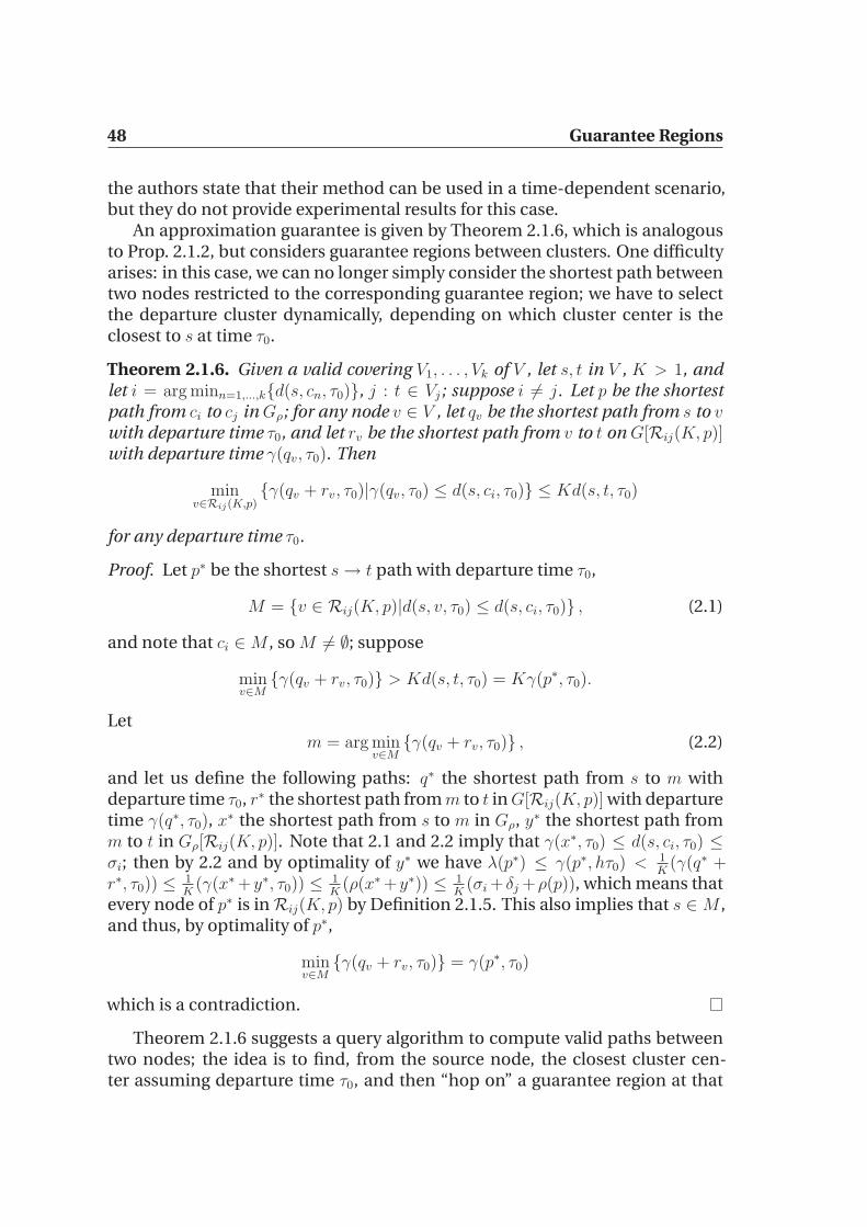
48 Guarantee Regions
the authors state that their method can be used in a time-dependent scenario,but they do not provide experimental results for this case.
An approximation guarantee is given by Theorem 2.1.6, which is analogousto Prop. 2.1.2, but considers guarantee regions between clusters. One difficultyarises: in this case, we can no longer simply consider the shortest path betweentwo nodes restricted to the corresponding guarantee region; we have to selectthe departure cluster dynamically, depending on which cluster center is theclosest to s at time τ0.
Theorem 2.1.6. Given a valid covering V1, . . . , Vk of V , let s, t in V , K > 1, andlet i = arg minn=1,...,k{d(s, cn, τ0)}, j : t ∈ Vj ; suppose i 6= j. Let p be the shortestpath from ci to cj in Gρ; for any node v ∈ V , let qv be the shortest path from s to vwith departure time τ0, and let rv be the shortest path from v to t on G[Rij(K, p)]with departure time γ(qv, τ0). Then
minv∈Rij(K,p)
{γ(qv + rv, τ0)|γ(qv, τ0) ≤ d(s, ci, τ0)} ≤ Kd(s, t, τ0)
for any departure time τ0.
Proof. Let p∗ be the shortest s→ t path with departure time τ0,
M = {v ∈ Rij(K, p)|d(s, v, τ0) ≤ d(s, ci, τ0)} , (2.1)
and note that ci ∈M , so M 6= ∅; suppose
minv∈M{γ(qv + rv, τ0)} > Kd(s, t, τ0) = Kγ(p∗, τ0).
Letm = arg min
v∈M{γ(qv + rv, τ0)} , (2.2)
and let us define the following paths: q∗ the shortest path from s to m withdeparture time τ0, r∗ the shortest path from m to t in G[Rij(K, p)] with departuretime γ(q∗, τ0), x∗ the shortest path from s to m in Gρ, y∗ the shortest path fromm to t in Gρ[Rij(K, p)]. Note that 2.1 and 2.2 imply that γ(x∗, τ0) ≤ d(s, ci, τ0) ≤σi; then by 2.2 and by optimality of y∗ we have λ(p∗) ≤ γ(p∗, hτ0) < 1
K(γ(q∗ +
r∗, τ0)) ≤1K
(γ(x∗+y∗, τ0)) ≤1K
(ρ(x∗+y∗)) ≤ 1K
(σi + δj +ρ(p)), which means thatevery node of p∗ is inRij(K, p) by Definition 2.1.5. This also implies that s ∈M ,and thus, by optimality of p∗,
minv∈M{γ(qv + rv, τ0)} = γ(p∗, τ0)
which is a contradiction.
Theorem 2.1.6 suggests a query algorithm to compute valid paths betweentwo nodes; the idea is to find, from the source node, the closest cluster cen-ter assuming departure time τ0, and then “hop on” a guarantee region at that

2.2 Computing the node sets 49
Figure 2.1: The label of each arc (u, v) is [λ(u, v), ρ(u, v)].
center. That is, if i is the index of the cluster whose center is the closest to sassuming departure time τ0, and j is the index of the cluster which contains t,then after settling ci we constrain the search to explore only nodes in the guar-antee region between Vi and Vj . Note that the computed shortest path does notnecessarily pass through ci, but the search is restricted to the guarantee regiononly after ci is settled. The query algorithm is described in Section 2.3.
A result similar to Prop. 2.1.3 holds for Rij(K, p∗) when p∗ ∈ P ∗ρ (ci, cj), andserves as a hint to choose our initial path. Unfortunately, guarantee regionsdefined this way may fail to be minimal.
Proposition 2.1.7. Given a valid covering V1, . . . , Vk of V , for i, j ≤ k, i 6= j let p∗
be the shortest path between ci and cj in Gρ, and p be another (different) ci → cj
path. If p∗ ⊂ Rij(K, p) thenRij(K, p∗) ⊆ Rij(K, p).
Example 2.1.8. We give an example of the fact that guarantee regions may fail tohave minimal size. We consider s = A, t = E,K = 6
5in the graph of Fig. 2.1. Since
the shortest path from A to E in Gρ is p∗ = (A,B,D,E), those nodes are includedin R(6/5, p∗). Furthermore, since ρ(A,B,D,E) = 270, and since the path p =(A,B,C,E) in Gλ has cost λ(p) = 224 < 5
6270 = 225, we have that R(6/5, p∗) =
{A,B,C,D,E}. However, it is easy to see that the set R′ = {A,B,D,E} has asmaller size and is enough to guarantee the approximation property.
2.2 Computing the node sets
By Definition 2.1.1 and Definition 2.1.5, it is clear that the most difficult (andexpensive) part during the computation of guarantee regions is determining allpaths q between s and t with λ-cost λ(q) < H, where H is a given value. H de-pends whether we are in the unclustered or in the clustered case. Computing Hitself is not computationally expensive: by Definition 2.1.5, we are interested inH = 1
K(ρ(p)+σi+δj) where p is the shortest path between ci and cj on Gρ. There-
fore, p can be obtained with an application of Dijkstra’s algorithm; similarly, σi
and δj can be calculated by growing shortest path trees from ci (respectively, cj)on Gρ (respectively, Gρ).

50 Guarantee Regions
We now propose an algorithm to compute the set of all nodes that belongto a path from a node s to a node t with total cost < H, adding some linesto Dijkstra’s algorithmm and applying it on the reverse graph (note that, withstraightforward changes, the same holds on the original graph). Let us definethe limited-width shortest paths tree Tu,L from a given node u of width L as theshortest paths tree that contains all nodes v such that dλ(u, v) < L. We callℓ[v] Dijkstra’s algorithm label of a node v ∈ Ts,L computed on the direct graph,i.e. ℓ[v] = dλ(u, v), and ℓ[v] Dijkstra’s algorithm label of a node v computed onthe reverse graph, i.e. ℓ[v] = dλ(v, u). We assume to set ℓ[v] = ∞ if v /∈ Ts,L, andℓ[v] =∞∀v ∈ V . Algorithm 1 computes the desired set.
Algorithm 1 Find all nodes on a path with total λ-cost < H from a node s toa node t
1: Build Ts,H on graph Gλ
2: Q← {t}3: ℓ[t]← 04: S ← ∅5: E ← ∅6: stop = false
7: if ℓ[t] 6=∞ then8: while Q 6= ∅ ∧ ¬stop do9: extract u← arg minq∈Q{ℓ[q]}
10: E ← E ∪ {u}11: if ℓ[u] + ℓ[u] < H then12: S ← S ∪ {u}13: if ℓ[u] ≥ H then14: stop = true
15: for all arcs (v, u) ∈ A do16: if v /∈ E then17: if v /∈ Q then18: ℓ[v]← ℓ[u] + λ(v, u)19: Q← Q ∪ {v}20: else if ℓ[u] + λ(v, u) < ℓ[v] then21: ℓ[v]← ℓ[u] + λ(v, u)22: return S
Proposition 2.2.1. Algorithm 1 returns all nodes on a path p from s to t such thatλ(p) < H.
Proof. First, we note that this algorithm is a modification of Dijkstra’s algorithmwhich adds some lines that do not interfere with the correctness of Dijkstra’salgorithm; there is one additional terminating condition on the main loop: thealgorithm stops if it has settled a node u with ℓ[u] > H.

2.3 Query algorithm 51
First part: Algorithm 1 returns all nodes on a path p from s to t such thatλ(p) < H. Suppose there is a node u /∈ S, u ∈ q where q is an s→ t path such thatλ(q) < H; since there is a path from s to t with cost < H, we have dλ(u, t) < H,so node u is scanned because the additional terminating condition on the mainloop does not apply. Also, we have that dλ(s, u) + dλ(u, t) ≤ λ(q) by optimality.Thus, when the node is scanned, the test on line 11 holds since ℓ[u] + ℓ[u] =dλ(s, u) + d(u, t) ≤ λ(q) < H, and u is added to S, which is a contradiction.
Second part: Algorithm 1 returns only nodes on a path p from s to t such thatλ(p) < H. Suppose there is a node u ∈ S such that 6 ∃q = (s, v1, . . . , vn, t) suchthat λ(q) < H, u ∈ q. Since u ∈ S, then it has been added on line 12; therefore,ℓ[u] + ℓ[u] < H. In this case, by definition of ℓ[u] and l[u], we can concatenatethe shortest paths from s to u and from u to t to build a s → t path with costℓ[u] + ℓ[u] < H. The contradiction follows.
Time requirements for Algorithm 1 are equivalent to applying two times Di-jkstra’s algorithm on the original graph, thus O(|A|+|V | log |V |) with Fibonacci’sheaps, but each application can be stopped as soon as we reach a distance of Hfrom source node. Hence, effective running time greatly depends on H, whichin turns depends on the choice of K and graph’s topology: the higher K, thelower the execution time. Space requirements are linear in |V |: in additionto Dijkstra’s algorithm linear space requirements, we only need to store eachnode’s label in the direct search before applying the reverse search. Note thatkeeping track of the whole shortest paths trees is not needed.
2.3 Query algorithm
Given a valid covering V1, . . . , Vk for V , Theorem 2.1.6 points at a way to com-pute a K-approximated time-dependent path between any pair of nodes s, t ∈V . Suppose we have already computed Rij(K, p∗) ∀i 6= j, 1 ≤ i, j ≤ k, andfor p∗ is the shortest path between ci and cj in Gρ; let us define Rii(K, p∗) =V ∀i, 1 ≤ i ≤ k. We will use a slightly modified version of time-dependentDijkstra’s algorithm, where we will call ℓ[v] Dijkstra’s algorithm label of a nodev ∈ V , and we denote by p[v] the parent node for node v. We assume to setℓ[v] :=∞, p[v] := nil ∀v ∈ V . Algorithm 2 respects the theorem’s conditions.
Proposition 2.3.1. Algorithm 2 computes a path p from s to t such that γ(p, τ0) ≤Kd(s, t, τ0).
Proof. First, note that Algorithm 2 is a modification of the time-dependent Di-jkstra’s algorithm, with an early termination condition which is known to becorrect: the algorithm stops as soon as the sink t has been settled, instead ofwaiting for the queue to be empty. We have to prove that the modifications donot interfere with the algorithm’s correctness.
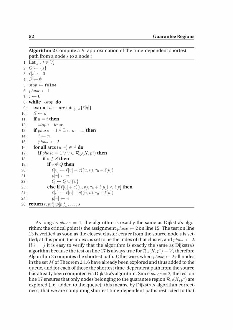
52 Guarantee Regions
Algorithm 2 Compute a K-approximation of the time-dependent shortestpath from a node s to a node t
1: Let j : t ∈ Vj
2: Q← {s}3: ℓ[s]← 04: S ← ∅5: stop ← false
6: phase ← 17: i ← 08: while ¬stop do9: extract u← arg minq∈Q{ℓ[q]}
10: S ← u11: if u = t then12: stop ← true
13: if phase = 1 ∧ ∃n : u = cn then14: i ← n15: phase ← 216: for all arcs (u, v) ∈ A do17: if phase = 1 ∨ v ∈ Rij(K, p∗) then18: if v /∈ S then19: if v /∈ Q then20: ℓ[v]← ℓ[u] + c((u, v), τ0 + ℓ[u])21: p[v]← u22: Q← Q ∪ {v}23: else if ℓ[u] + c((u, v), τ0 + ℓ[u]) < ℓ[v] then24: ℓ[v]← ℓ[u] + c((u, v), τ0 + ℓ[u])25: p[v]← u26: return t, p[t], p[p[t]], . . . , s
As long as phase = 1, the algorithm is exactly the same as Dijkstra’s algo-rithm; the critical point is the assignment phase ← 2 on line 15. The test on line13 is verified as soon as the closest cluster center from the source node s is set-tled; at this point, the index i is set to be the index of that cluster, and phase ← 2.If i = j it is easy to verify that the algorithm is exactly the same as Dijkstra’salgorithm because the test on line 17 is always true forRii(K, p∗) = V , thereforeAlgorithm 2 computes the shortest path. Otherwise, when phase ← 2 all nodesin the set M of Theorem 2.1.6 have already been explored and thus added to thequeue, and for each of those the shortest time-dependent path from the sourcehas already been computed via Dijkstra’s algorithm. Since phase = 2, the test online 17 ensures that only nodes belonging to the guarantee regionRij(K, p∗) areexplored (i.e. added to the queue); this means, by Dijkstra’s algorithm correct-ness, that we are computing shortest time-dependent paths restricted to that
2.4 Implementation 53
node set. However, these are exactly the conditions of Theorem 2.1.6, and thuswhen node t is settled we have computed a path which is the optimum of
minv∈Rij(K,p)
{γ(qv + rv, τ0)|γ(qv, τ0) ≤ d(s, ci, τ0)} ≤ Kd(s, t, τ0)
for any departure time τ0.
In order to provide an upper bound on the computational time of each short-est path computation, we have to provide an upper bound on the number ofnodes that are explored. The required upper bound on computational time canthen be derived considering the maximum time spent per node (i.e. while set-tling the node with maximum degree in the graph) and the maximum time fora priority queue operation. It is straightforward to note that, once Algorithm2 has switched to phase 2, then the number of nodes that can be explored isbounded from above by |Rij(K, p∗)| + |Vj|, where i and j are, respectively, theindex of the source and of the destination cluster. We have to provide a boundon the number of nodes explored before switching to phase 2: in order to do sowe note that, if we restrict the algorithm in phase 1 to explore only nodes withinVi, where s ∈ Vi, then the approximation guarantee is still valid, although thesolution quality may decrease. Thus we require that, if b nodes have alreadybeen explored in phase 1, then the algorithm is restricted to explore only nodesin Vi, until it switches to phase 2. It is easy to prove correctness of this approach.An upper bound on the number of explored nodes is then
b + |Vi|+ |Rij(K, p∗)|+ |Vj|. (2.3)
The size ofRij(K, p∗) can be decreased by increasing K.
2.4 Implementation
To validate the practical usefulness of this approach, we implemented it in theC++ programming language. It turns out that performance is not fully satisfy-ing. In this section we report our results.
2.4.1 Storing node sets
Once all guarantee regions have been computed with the algorithm describedin Section 2.2, we have to store them efficiently in memory for a fast access. Thisissue is crucial for performance, since the query algorithm has to test, for eachnode, whether it belongs to a given guarantee region or not, and thus the algo-rithm’s efficiency depends on how quickly this answer can be given and howaccurately node sets are stored. Assuming that we know each node’s position
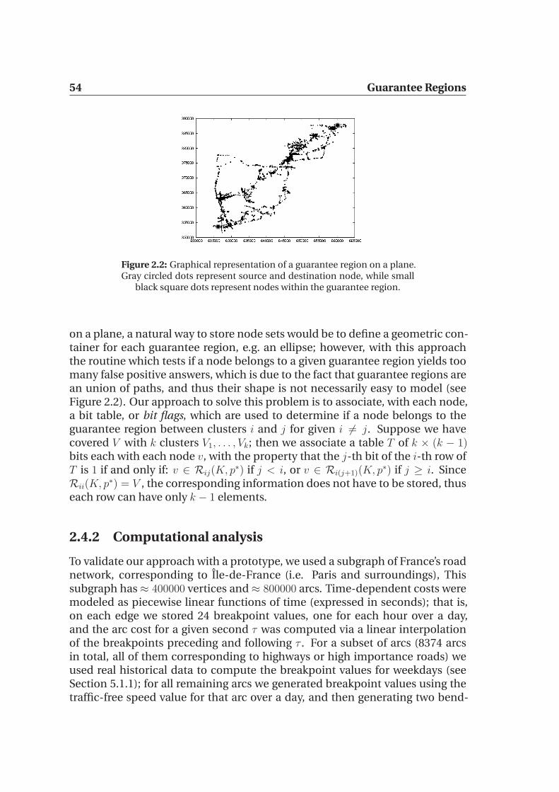
54 Guarantee Regions
Figure 2.2: Graphical representation of a guarantee region on a plane.Gray circled dots represent source and destination node, while small
black square dots represent nodes within the guarantee region.
on a plane, a natural way to store node sets would be to define a geometric con-tainer for each guarantee region, e.g. an ellipse; however, with this approachthe routine which tests if a node belongs to a given guarantee region yields toomany false positive answers, which is due to the fact that guarantee regions arean union of paths, and thus their shape is not necessarily easy to model (seeFigure 2.2). Our approach to solve this problem is to associate, with each node,a bit table, or bit flags, which are used to determine if a node belongs to theguarantee region between clusters i and j for given i 6= j. Suppose we havecovered V with k clusters V1, . . . , Vk; then we associate a table T of k × (k − 1)bits each with each node v, with the property that the j-th bit of the i-th row ofT is 1 if and only if: v ∈ Rij(K, p∗) if j < i, or v ∈ Ri(j+1)(K, p∗) if j ≥ i. SinceRii(K, p∗) = V , the corresponding information does not have to be stored, thuseach row can have only k − 1 elements.
2.4.2 Computational analysis
To validate our approach with a prototype, we used a subgraph of France’s roadnetwork, corresponding to Ile-de-France (i.e. Paris and surroundings), Thissubgraph has≈ 400000 vertices and≈ 800000 arcs. Time-dependent costs weremodeled as piecewise linear functions of time (expressed in seconds); that is,on each edge we stored 24 breakpoint values, one for each hour over a day,and the arc cost for a given second τ was computed via a linear interpolationof the breakpoints preceding and following τ . For a subset of arcs (8374 arcsin total, all of them corresponding to highways or high importance roads) weused real historical data to compute the breakpoint values for weekdays (seeSection 5.1.1); for all remaining arcs we generated breakpoint values using thetraffic-free speed value for that arc over a day, and then generating two bend-
2.4 Implementation 55
ings in the speed profile so as to slow the arc down by a factor of 1.5–3 duringpeak hours, with each drop lasting 3-5 hours and centered at 8 AM or 6 PM.This empirical way to generate time-dependent costs was not meant to be com-pletely realistic, but at least it should provide “reasonable” data. Then, for eachquery, we randomly generated with a uniform distribution a departure time inseconds between 7 AM and 7 PM, so that the optimal time-dependent solutionhas a very high probability of being different than the traffic-free static solution.
To validate the clustered approach we generated a k-center clustering overV , with k = 100 clusters, using k′-oversampling with k′ = 200 (see (103)); that is,we picked 200 random nodes, we connected them to a “dummy” central node,and we grew clusters of neighbouring nodes around each of the 200 centers.Then, when all nodes had been assigned to a cluster, we progressively deletedthe smallest remaining cluster, i.e. the one with the smallest radius, allowingother clusters to grow into the deleted one. We iterated this procedure until100 clusters were left. We compared the number of explored and settled nodesbetween a Dijkstra search and Algorithm 2, where source and destination nodewere chosen at random. We also compared the results with respect to the naivealgorithm of computing the shortest path in the static traffic-free graph, i.e. Gλ,and then applying time-dependent costs. Results are reported in Table 2.1. Foreach value of K (first column), we indicate the average number of settled nodesin 1000 Dijkstra searches on the full graph, the average number of settled nodeswith Algorithm 2 and the same source-destination pairs, the average percent-age increase P of the naive solution value with respect to the optimum (thatis, if p∗ is the optimal solution and p is the naive solution, the average valueof (1− γ(p, τ0)/γ(p∗, τ0))), the average percentage increase of the approximatedsolution value with respect to the optimum, the average CPU time savings ofAlgorithm 2 in percentage of the CPU times saved with respect to the exact al-gorithm (0% means as slow as the exact algorithm; a negative value means thatthere is an increase in CPU time, while a positive value means that CPU time de-creased), and the percentage of shortest path computations where the approxi-mated a solution had a cost smaller or equal than the cost of the naive solution.We do not provide exact query times because those are highly dependent onthe implementation, and in this case our implementation was not fine-tuned;what is most interesting, here, is the speed-up with respect to plain Dijkstra’salgorithm in terms of number of settled nodes and of relative CPU time. Thenumber of settled nodes for the naive approach is not relevant: many speed-up techniques exist for the static case (see Section 1.4), so we can assume thatit is a fast computation. While for low values of K computational times couldincrease, due to the overhead for constraining the Dijkstra search within theboundaries of the guarantee region, for high enough values of the approxima-tion constant the savings in CPU time are significant, with a small average de-crease of the solution quality with respect to the optimum. For K ≤ 3, there isno speedup in the computation. Therefore, this method requires a very large

56 Guarantee Regions
MAX # SETTLED NODES SOLUTION COST INCREASE CPU TIME IMPROVED
K DIJKSTRA APPROX NAIVE APPROX SAVINGS PATHS
3 185514 60045 4.56% 1.10% 53.99% 91.8%3.5 194640 35561 4.43% 4.91% 74.66% 74.5%
4 190077 15597 4.58% 9.27% 87.69% 53.2%4.5 193240 9943 4.46% 16.51% 91.51% 38.2%
3.5∗ 188988 29341 4.38% 1.75% 78.22% 76.4%4∗ 184327 17256 4.79% 4.54% 86.28% 67.2%
4.5∗ 190944 12675 4.40% 5.40% 91.72% 58.2%
Table 2.1: Computational results on clustered graph: average values. A∗ in the first column indicates that the value for K has been adaptivelychosen, and we report the starting value, which is also the maximum
one.
approximation constant to bring practical benefits, although the solution qual-ity is in practice significantly closer to the optimum than the approximationconstant would allow. We note, however, that the naive solution has a betteraverage behaviour than our approximated solution for values of K ≥ 3.5. Wetried to investigate the reason behind this. We can see that, for K = 3.5, in74.5% of the shortest path computations the approximated solution is betterthan the naive one, but in the remaining cases the approximated solution isvery far from the optimum, while the naive one isn’t. This is due to the fact that,if K is too large, then the guarantee region between two clusters i and j mayconsist of only the shortest path between ci and cj on Gµ. Any approximatedsolution between those two clusters will pass through that path, which leadsto poor performance. For K = 3, in 91.8% of the shortest path computationsthe approximated solution has a cost which is smaller than the cost of the naivesolution, so the average behaviour of the approximated solution is satisfying.However, the computation is only 54% faster than a full (unconstrained) Dijk-stra search.
To deal with this issue, we adaptively chose the value of the approximationconstant K as follows: for each cluster pair, we started with the maximumvalue for K (Kcurr ← Kmax), and if the computed guarantee region includedonly the path between the cluster centers we decreased the current K by 10%(Kcurr ← 0.9Kcurr). We iterated until the guarantee region for that cluster pairhad a cardinality which was greater than the number of nodes on the shortestpath on Gµ between the cluster centers. Results for this approach are reportedin Table 2.1, on the rows with a ∗ in the first column.
With this modification in the guarantee region generation process, we seethat the solution quality significantly increases, while still yielding a speed-upin computational time. Moreover, we are able to obtain a better average be-
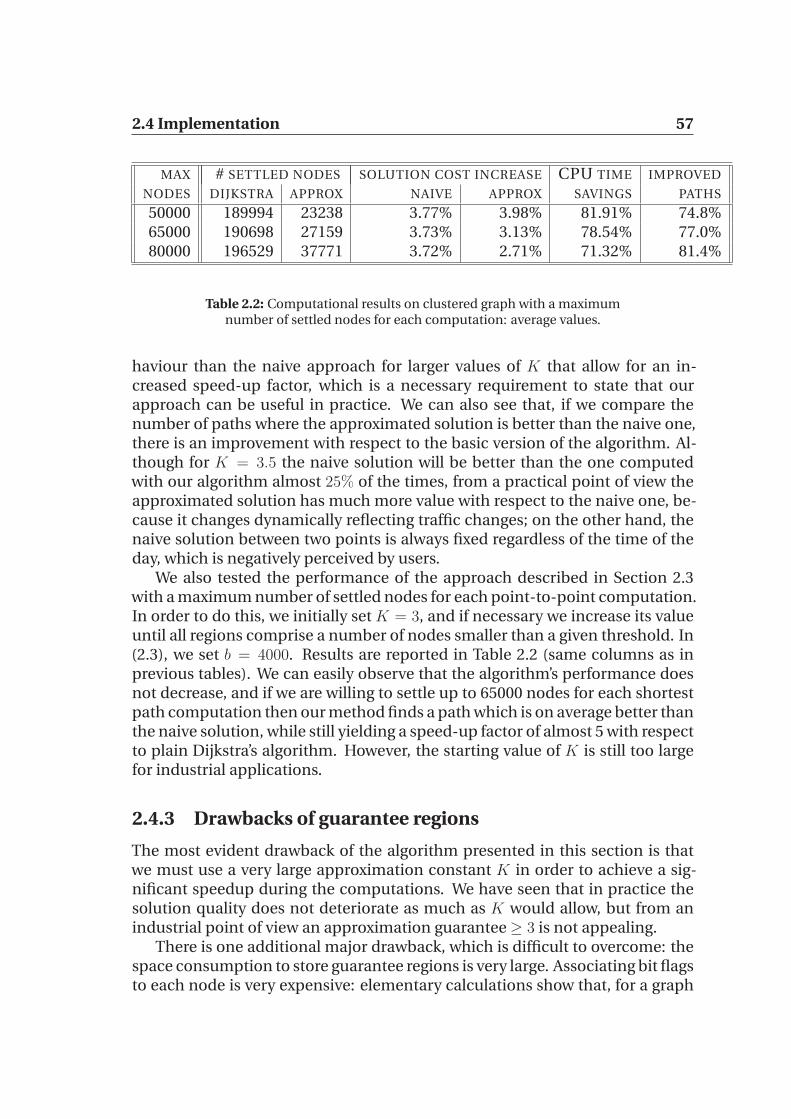
2.4 Implementation 57
MAX # SETTLED NODES SOLUTION COST INCREASE CPU TIME IMPROVED
NODES DIJKSTRA APPROX NAIVE APPROX SAVINGS PATHS
50000 189994 23238 3.77% 3.98% 81.91% 74.8%65000 190698 27159 3.73% 3.13% 78.54% 77.0%80000 196529 37771 3.72% 2.71% 71.32% 81.4%
Table 2.2: Computational results on clustered graph with a maximumnumber of settled nodes for each computation: average values.
haviour than the naive approach for larger values of K that allow for an in-creased speed-up factor, which is a necessary requirement to state that ourapproach can be useful in practice. We can also see that, if we compare thenumber of paths where the approximated solution is better than the naive one,there is an improvement with respect to the basic version of the algorithm. Al-though for K = 3.5 the naive solution will be better than the one computedwith our algorithm almost 25% of the times, from a practical point of view theapproximated solution has much more value with respect to the naive one, be-cause it changes dynamically reflecting traffic changes; on the other hand, thenaive solution between two points is always fixed regardless of the time of theday, which is negatively perceived by users.
We also tested the performance of the approach described in Section 2.3with a maximum number of settled nodes for each point-to-point computation.In order to do this, we initially set K = 3, and if necessary we increase its valueuntil all regions comprise a number of nodes smaller than a given threshold. In(2.3), we set b = 4000. Results are reported in Table 2.2 (same columns as inprevious tables). We can easily observe that the algorithm’s performance doesnot decrease, and if we are willing to settle up to 65000 nodes for each shortestpath computation then our method finds a path which is on average better thanthe naive solution, while still yielding a speed-up factor of almost 5 with respectto plain Dijkstra’s algorithm. However, the starting value of K is still too largefor industrial applications.
2.4.3 Drawbacks of guarantee regions
The most evident drawback of the algorithm presented in this section is thatwe must use a very large approximation constant K in order to achieve a sig-nificant speedup during the computations. We have seen that in practice thesolution quality does not deteriorate as much as K would allow, but from anindustrial point of view an approximation guarantee≥ 3 is not appealing.
There is one additional major drawback, which is difficult to overcome: thespace consumption to store guarantee regions is very large. Associating bit flagsto each node is very expensive: elementary calculations show that, for a graph

58 Guarantee Regions
with 18M nodes such as the European road network (Section 5.1), 8GB of mem-ory would allow only ≈ 60 clusters in the graph covering. In this case, eachcluster would be very large, hence performance would significantly decrease.More efficient methods for identifying nodes belonging to a guarantee regioncould be devised, but, as discussed in Section 2.4.1, one has to be careful notto introduce too many false positives. In the end, we decided to try a differentapproach, in which the set of nodes to be explored is not predetermined andstored in memory, but is computed “on-the-fly” for each shortest path query.This way, there is no additional space consumption for the storage of guaran-tee regions.

Chapter 3
Bidirectional A∗ Search onTime-Dependent Graphs
Bidirectional search is an important tool for the development of speedup tech-niques for the SPP on static graphs; however, it cannot be directly applied ontime-dependent graphs. In this section we propose a novel algorithm for theTDSPP based on a bidirectional A∗ algorithm. Since the arrival time is notknown in advance (so c cannot be evaluated on the arcs adjacent to the des-tination node), our backward search occurs on the graph weighted by the lowerbounding function λ. This is used for bounding the set of nodes that will beexplored by the forward search.
The rest of this chapter is organized as follows. In Section 3.1 we describethe foundations of our idea, and present an adaptation of the ALT algorithmbased on it. In Section 3.2 we formally prove our method’s correctness. In Sec-tion 3.3 we propose some modifications that improve the performance of ouralgorithm, and prove their correctness. In Section 3.4 we discuss the dynamiccase, where arc cost functions are allowed to change under weak conditions.
3.1 Algorithm description
We propose a general approach for bidirectional search based on restricting thescope of a time-dependent A∗ search from the source using a set of nodes de-fined by a time-independent A∗ search from the destination, i.e. the backwardsearch is a reverse search in Gλ. This idea is related to the guarantee regions dis-cussed in Chapter 2: in that case we predetermined the set of nodes that hadto be explored for each shortest path computation, while this approach triesto identify such nodes “on-the-fly”, depending on the source and destinationnode. Note that Dijkstra’s algorithm is equivalent to A∗ with a zero potentialfunction; thus, in the following we could use Dijkstra’s algorithm instead of A∗.However, as A∗ already yields a reduced search space with respect to Dijkstra’s

60 Bidirectional A∗ Search on Time-Dependent Graphs
s t
(a) Phase 1
s t
(b) From Phase 1 to Phase 2
s t
(c) Phase 2
s t
(d) Phase 3
Figure 3.1: Schematic representation of the TDALT algorithm searchspace
algorithm, we will assume that the first algorithm is used, even though all theo-retical properties also hold for Dijkstra’s algorithm.
Given a graph G = (V,A) and source and destination vertices s, t ∈ V , the al-gorithm for computing the shortest time-dependent cost path p∗ works in threephases.
1. A bidirectional A∗ search occurs on G, where the forward search is runon the graph weighted by c, and the backward search is run on the graphweighted by the lower bounding function λ. All nodes settled by the back-ward search are included in a set M . Phase 1 terminates as soon as thetwo search scopes meet.

3.2 Correctness 61
2. Suppose that v ∈ V is the first vertex in the intersection of the heaps of theforward and backward search; then the time dependent cost µ = γ(pv, τ0)of the path pv going from s to t passing through v is an upper bound toγ(p∗, τ0). In the second phase, both search scopes are allowed to proceeduntil the backward search queue only contains nodes whose associatedkey exceeds µ. In other words: let β be the key of the minimum element ofthe backward search queue; phase 2 terminates as soon as β > µ. Again,all nodes settled by the backward search are included in M .
3. Only the forward search continues, with the additional constraint thatonly nodes in M can be explored. The forward search terminates whent is settled.
If the ALT algorithm (Section 1.4.5.1) is used for the A∗ search, i.e. we use land-mark potential functions, then we call this algorithm TIME-DEPENDENT ALT( TDALT). The pseudocode is given in Algorithm 3. Note that we use the symbol↔ to indicate either the forward search (↔=→) or the backward search (↔=←):as a consequence, −→π is the potential function for the forward search, while←−πis the potential function for the backward search. Similarly for all other iden-
tifiers. We denote by−→A the set of arcs for the forward search, i.e.
−→A = A, and
by←−A the set of arcs for the backward search, i.e.
←−A = A. A typical choice is
to alternate between the forward and the backward search at each iteration ofthe algorithm during the first two phases. Through the rest of this work we willalways alternate between the two searches at each iteration.
We give a sketch of the algorithm in Figure 3.1. In Figure 3.1(a) the algorithmis in Phase 1: a forward search starts on the time-dependent graph and a back-ward search starts on the same graph weighted by the lower bounding functionλ. As soon as the two search scopes meet (Figure 3.1(b)), we compute an upperbound µ on the cost of optimal solution by evaluating the time-dependent costof an s → t path, and switch to Phase 2. In Figure 3.1(c) the algorithm is inPhase 2: both searches continue until the condition β > µ is verified, where βis the minimum element of the backward search priority queue. When the con-dition holds, the algorithm switches to Phase 3 (Figure 3.1(d)): the backwardsearch stops, and the forward search continues until the target node is settled,but the forward search is allowed to explore only nodes already settled by thebackward search.
3.2 Correctness
We prove correctness of our approach for the computation of both optimal so-lutions and suboptimal solutions with an approximation guarantee.
Theorem 3.2.1. Algorithm 3 computes the shortest time-dependent path from sto t for a given departure time τ0.

62 Bidirectional A∗ Search on Time-Dependent Graphs
Algorithm 3 TDALT: Compute the shortest time-dependent path from s to twith departure time τ0−→Q.insert(s, 0);
←−Q.insert(t, 0); M := ∅; µ := +∞; done := false; phase := 1.
while ¬done doif (phase = 1) ∨ (phase = 2) then↔∈ {→,←}
else↔:=→
u :=←→Q .extractMin()
if (u = t) ∧ (↔=→) thendone := true
continueif (phase = 1) ∧ (u.dist→ + u.dist← <∞) then
µ := u.dist→ + u.dist←
phase := 2if (phase = 2) ∧ (↔=←) ∧ (µ < u.key←) then
phase := 3continue
for all arcs (u, v) ∈←→A do
if↔=← thenM.insert(u)
else if (phase = 3) ∧ (v /∈M) thencontinue;
if (v ∈←→Q ) then
if u.dist↔ + c(u, v, u.dist↔) < v.dist↔ then←→Q .decreaseKey(v, u.dist↔ + c(u, v, u.dist↔) +←→π (v))
else←→Q .insert(v, u.dist↔ + c(u, v, u.dist↔) +←→π (v))
return t.dist→
Proof. The forward search of Algorithm 3 is exactly the same as the unidirec-tional version of the A∗ algorithm during the first 2 phases, and thus it is correct;we have to prove that the restriction applied during phase 3 does not interferewith the correctness of the A∗ algorithm.
Let µ be an upper bound on the cost of the shortest path; in particular, thiscan be the cost γ(pv, τ0) of the s→ t path passing through the first meeting pointv of the forward and backward search. Let β be the smallest key of the backwardsearch priority queue at the end of phase 2. Suppose that Algorithm 3 is notcorrect, i.e. it computes a sub-optimal path. Let p∗ be the shortest path from sto t with departure time τ0, and let u be the first node on p∗which is not exploredby the forward search; by phase 3, this implies that u /∈ M , i.e. u has not beensettled by the backward search during the first 2 phases of Algorithm 3. Hence,

3.3 Improvements 63
we have that β ≤ πb(u) + dλ(u, t); then we have the chain γ(p∗, τ0) ≤ µ < β ≤πb(u)+ dλ(u, t) ≤ dλ(s, u)+ dλ(u, t) ≤ d(s, u, τ0)+ d(u, t, τ0 + d(s, u, τ0)) = γ(p∗, τ0),which is a contradiction.
Theorem 3.2.2. Let p∗ be the shortest path from s to t. If the condition to switchto phase 3 is µ < Kβ for a fixed parameter K, then Algorithm 3 computes a pathp from s to t such that γ(p, τ0) ≤ Kγ(p∗, τ0) for a given departure time τ0.
Proof. Suppose that γ(p, τ0) > Kγ(p∗, τ0). Let u be the first node on p∗ whichis not explored by the forward search; by phase 3, this implies that u /∈ M ,i.e. u has not been settled by the backward search during the first 2 phasesof Algorithm 3. Hence, we have that β ≤ πb(u) + dλ(u, t); then we have thechain γ(p, τ0) ≤ µ < Kβ ≤ K(πb(u) + dλ(u, t)) ≤ K(dλ(s, u) + dλ(u, t)) ≤K(d(s, u, τ0)+d(u, t, τ0 +d(s, u, τ0))) = Kγ(p∗, τ0) < γ(p, τ0), which is a contradic-tion.
3.3 Improvements
Performance of the basic version of the algorithm can be improved with theresults that we describe in this section, whose purpose is to reduce further thesize of the search space.
Theorem 3.3.1. Let p be the shortest path from s to t with departure time τ0. Ifall nodes u on p settled by the backward search are settled with a key smaller orequal to d(s, u, τ0) + d(u, t, τ0 + d(s, u, τ0)), then Algorithm 3 is correct.
Proof. Let Q be the backward search queue, let key(u) be the key for the back-ward search of node u, let β = minu∈Q{key(u)} be the smallest key in the back-ward search queue, which is attained at a node v (i.e. v = arg minu∈Q{key(u)}),and let µ the best upper bound on the cost of the solution currently known. Toprove correctness, using the same arguments as in the proof of Theorem 3.2.1we must make sure that, when the backward search stops at the end of phase2, then all nodes on the shortest path from s to t that have not been exploredby the forward search have been added to M . The backward search stops whenµ < β.
In an A∗ search, the keys of settled nodes are non-decreasing. So every nodeu which at the current iteration has not been settled by the backward searchwill be settled with a key key(u) ≥ key(v), which yields d(s, u, τ0) + d(u, t, τ0 +d(s, u, τ0)) ≥ key(v) = β > µ ∀u ∈ Q. Thus, every node which has not beensettled by the backward search cannot be on the shortest path from s to t, andAlgorithm 3 is correct.

64 Bidirectional A∗ Search on Time-Dependent Graphs
This allows the use of larger lower bounds during the backward search: thebackward A∗ search does not have to compute shortest paths on the graph Gλ,but it should in any case guarantee that when a node u is settled then its key isan underestimation of the time-dependent cost of the time-dependent shortestpath between s and t passing through u. The next proposition is of fundamentalpractical importance.
Proposition 3.3.2. In phase 2 of Algorithm 3, nodes that have already been set-tled by the forward search do not have to be explored by the backward search.
Proof. Let db(v) be the distance from a node v to node t computed by the back-ward search if we do not explore any node already explored by the forwardsearch. Obviously we have db(v) ≥ dλ(v, t). We will prove that, when a nodev on the shortest path from s to t with departure time τ0 is settled by the back-ward search, then db(v) ≤ d(v, t, τ0 + d(s, v, τ0)) ∀τ0 ∈ T . By Theorem 3.3.1, thisis enough to prove our statement.
Consider a node v settled by the backward search, but not by the forwardsearch; let q be the shortest path from s to v with departure time τ0, let q′ bethe shortest path from v to t with departure time tau0 + γ(q, τ0). Suppose thatq′ does not pass through any node already settled by the forward search. Thendb(v) ≤ λ(q′) ≤ d(v, t, τ0 + d(s, v, τ0)).
Suppose now that q′ passes through a node w already settled by the forwardsearch. Let p be the shortest path from s to w with departure time τ0, and let p′
be the shortest path from w to t with departure time τ0+γ(p, τ0); clearly v cannotbe on p, because otherwise it would have been settled by the forward search. Byoptimality of p we have γ(p, τ0) ≤ γ(q+q′|v→w, τ0) = γ(q, τ0)+γ(q′|v→w, τ0+γ(q, τ0)).
Thus, by the FIFO property, we have the chain γ(p + p′, τ0) = γ(p, τ0) + γ(p′, τ0 +γ(p, τ0)) ≤ γ(q, τ0) + γ(q′|v→w, τ0 + γ(q, τ0)) + γ(q′|w→t, τ0 + γ(q, τ0) + γ(q′|v→w, τ0 +
γ(q, τ0))) = γ(q + q′, τ0), which means that v does not have to be explored andadded to the set M by the backward search, because we already have a betterpath passing through w. Thus, even if key(v) > d(s, v, τ0) + d(v, t, τ0 + d(s, v, τ0))Algorithm 3 is correct.
By Theorem 3.3.1, we can take advantage of the fact that the backward searchis used only to bound the set of nodes explored by the forward search. Thismeans that we can tighten the bounds used by the backward search, even ifdoing so would result in an A∗ backward search that computes suboptimal dis-tances. To derive some valid lower bounds we need the following lemma andpropositions.
Lemma 3.3.3. Let v be a node, and u its parent node in the shortest path from sto v with departure time τ0. Then d(s, u, τ0) + πf (u) ≤ d(s, v, τ0) + πf (v).
Proof. Suppose that ℓ is the active landmark, i.e. the landmark in our landmarksset that currently gives the best bound; we have that either πf (u) = dλ(u, ℓ) −dλ(t, ℓ) or πf (u) = dλ(ℓ, t)− dλ(ℓ, u).

3.3 Improvements 65
First case: πf (u) = dλ(u, ℓ)− dλ(t, ℓ). We have d(s, u, τ0) + πf (u) = d(s, u, τ0) +dλ(u, ℓ)− dλ(t, ℓ) ≤ d(s, u, τ0) + dλ(u, v) + dλ(v, ℓ)− dλ(t, ℓ) ≤ d(s, u, τ0) + λ(u, v) +dλ(v, ℓ)− dλ(t, ℓ) ≤ d(s, v, τ0) + πf (v).
Second case: πf (u) = dλ(ℓ, t)−dλ(ℓ, u). We have d(s, u, τ0)+πf (u) = d(s, u, τ0)+dλ(ℓ, t)− dλ(ℓ, u); by triangular distance, dλ(ℓ, v) ≤ dλ(ℓ, u) + dλ(u, v) ≤ dλ(ℓ, u) +λ(u, v), which yields −dλ(ℓ, u) ≤ −dλ(ℓ, v) + λ(u, v). So d(s, u, τ0) + dλ(ℓ, t) −dλ(ℓ, u) ≤ d(s, u, τ0) + dλ(ℓ, t)− dλ(ℓ, v) + λ(u, v) ≤ d(s, v, τ0) + πf (v).
Proposition 3.3.4. At a given iteration, let v be the last node settled by the for-ward search. Then, for each node w which has not been settled by the forwardsearch, d(s, v, τ0) + πf (v)− πf (w) ≤ d(s, w, τ0).
Proof. There are two possibilities for w: either it has been explored (but notsettled) by the forward search, or it has not been explored. Let Q be the setof nodes in the forward search queue. If w has been explored, then w ∈ Q,and clearly d(s, v, τ0) + πf (v) ≤ d(s, w, τ0) + πf (w) because v has been extractedbefore w, which proves our statement. Otherwise, there is a node u ∈ Q on theshortest path from s to w with departure time τ0 which has been explored butnot settled. We have that d(s, v, τ0) + πf (v) ≤ d(s, u, τ0) + πf (u) because v hasbeen extracted while u is still in the queue, and by Lemma 3.3.3, if we examinethe nodes u = u1, u2, . . . , uk = w on the shortest path from s to w with departuretime τ0, we have that d(s, u1, τ0)+πf (u1) ≤ · · · ≤ d(s, uk, τ0)+πf (uk), from whichour statement follows.
Let v be as in Proposition 3.3.4, and w a node which has not been settled bythe forward search. Proposition 3.3.4 suggests that we can use
π∗b (w) = max{πb(w), d(s, v, τ0) + πf (v)− πf (w)} (3.1)
as a lower bound to d(s, w, τ0) during the backward search. However, we haveto make sure that the bound is valid at each iteration of Algorithm 3.
Lemma 3.3.5. If the key of the forward search used to compute the potentialfunction π∗b defined by (3.1) is fixed, then we have π∗b (v) ≤ π∗b (u) + λ(u, v) foreach arc (u, v) ∈ A.
Proof. By definition we have π∗b (v) = max{πb(v), α − πf (v)}, where with α wedenoted the key of a node settled by the forward search, which is fixed by hy-pothesis. Consider the case π∗b (v) = πb(v); then, since the landmark potentialfunctions πb and πf are consistent, we have π∗b (v) = πb(v) ≤ πb(u) + λ(u, v) ≤π∗b (u) + λ(u, v). Now consider the case π∗b = α − πf (v); then we have π∗b (v) =α−πf (v) ≤ α−πf (u)+λ(u, v) ≤ π∗b (u)+λ(u, v), which completes the proof.
This is enough to prove correctness of our algorithm with tightened bounds,as stated in the next theorem.

66 Bidirectional A∗ Search on Time-Dependent Graphs
Theorem 3.3.6. If we use the potential function π∗b defined by (3.1) as potentialfunction for the backward search, with a fixed value of the forward search key,then Algorithm 3 is correct.
Proof. Let db(u) be the distance from a node u to node t computed by the back-ward search. We will prove that, when a node u on the shortest path from s tot is settled by the backward search, db(u) ≤ d(u, t, τ0 + d(s, u, τ0)) ∀τ0 ∈ T . ByProposition 3.3.4 and Theorem 3.3.1, this is enough to prove our statement.
Let q∗ = (v1 = u, . . . , vn = t) be the shortest path from u to t on Gλ. Weproceed by induction on i : n, . . . , 1 to prove that each node vi is settled withthe correct distance on Gλ, i.e. db(vi) = dλ(vi, t). It is trivial to see that the nodesvn and vn−1 are settled with the correct distance on Gλ. For the induction step,suppose vi is settled with the correct distance db(vi) = dλ(vi, t). By Lemma 3.3.5,we have db(vi) + π∗b (vi) ≤ db(vi) + λ(vi−1, vi) + π∗b (vi−1) = dλ(vi−1, t) + π∗b (vi−1) ≤db(vi−1) + π∗b (vi−1), hence vi is extracted from the queue before vi−1. This meansthat vi−1 will be settled with the correct distance db(vi−1) = dλ(vi−1, t), and theinduction step is proven.
Thus, u will be settled with distance db(u) = dλ(u, t) ≤ d(u, t, τ0 + d(s, u, τ0)),which proves our statement.
By Theorem 3.3.6, Algorithm 3 is correct when using π∗b only if we assumethat the node v used in (3.1) is fixed at each backward search iteration. Thus, inpractice we do the following: we set up kmax ∈ N checkpoints during the query;when a checkpoint is reached, the node v used to compute (3.1) is updated,and the backward search queue is flushed and filled again using the updatedπ∗b . This is enough to guarantee correctness. The checkpoints are computedcomparing the initial lower bound ∆ = πf (t) and the current distance from thesource node, both for the forward search: the initial lower bound is divided bykmax and, whenever the current distance from the source node exceeds k∆/kmax
with k ∈ {1, . . . , kmax}, π∗b is updated.
3.4 Dynamic cost updates
Up to now, time-dependent routing algorithms assumed complete knowledgeof the time-dependent cost functions on arcs. However, since the speed profileson which these functions are based are generated using historical data gatheredfrom sensors (or cams), it is reasonable to assume that also real-time traffic in-formation is available through these sensors. Moreover, other technologies ex-ist to be aware of traffic jams even without having access to real-time speed in-formation (e.g., TMC1). In the end, a procedure to update the time-dependentcost functions depending on real-time traffic information would be desirablefor practical applications.
1http://www.tmcforum.com/

3.4 Dynamic cost updates 67
The input required by the TDALT algorithm (Section 3.1) consists of thegraph G with the associated arc cost functions and the distances to and fromlandmarks. As landmark distances are computed using the lower boundingfunction λ, it is clear that the preprocessing information, i.e. landmark distances,remain valid as long as λ = c, that is, λ bounds c from below. On road networks,computing a lower bounding function which is necessarily valid can be easilydone: it suffices to divide the length of the road segment that an arc representsby the maximum speed allowed on that type of road. Thus, as long as λ = c,the time-dependent cost functions can be updated with no additional requiredeffort.

68 Bidirectional A∗ Search on Time-Dependent Graphs
Chapter 4
Core Routing on Time-DependentGraphs
Hierarchical speedup techniques have been successfully used for the SPP onstatic graphs (Section 1.4.4), hence in this section we generalize these tech-niques to the time-dependent scenario and analyse performance of a two-levelhierarchical setup (core routing) for the TDSPP. The idea behind core routingis to shrink the original graph in order to get a new graph (core) with a smallernumber of vertices. Most of the search is then carried out on the core, yieldinga reduced search space. We combine core routing with the bidirectional goal-directed algorithm TDALT.
The rest of this section is organized as follow. In Section 4.1 we describecore routing on static graphs and generalize it to the time-dependent case. InSection 4.2 we discuss several issues that arise during the practical implemen-tation of a core-based algorithm, and propose solutions. In Section 4.3 we anal-yse under which conditions core optimality can be rapidly restored in the caseof updates in the cost functions, and propose an algorithm for this task. Finally,in Section 4.4 we discuss the extension of a two-levels approach to a multilevelhierarchy.
4.1 Algorithm description
Core-based routing is a powerful approach which has been widely and success-fully used for shortest paths algorithms on static graphs (Section 1.4.4. Themain idea is to use contraction (Section 1.4.4.3): a routine iteratively removesunimportant nodes and adds edges to preserve correct distances between theremaining nodes, so that we have a smaller network where most of the searchcan be carried out. Note that in principle we can use any contraction routinewhich removes nodes from the graph and inserts edges to preserve distances.When the contracted graph GC = (VC , AC) has been computed, it is merged
70 Core Routing on Time-Dependent Graphs
with the original graph to obtain GF = GC ∪G = (V,A ∪ AC) since VC ⊂ V .Suppose that we have a contraction routine which works on a time-dependent
graph: that is, ∀u, v ∈ VC , for each departure time τ0 ∈ T there is a shortest pathbetween u and v in GC with the same cost as the shortest path between u and vin G with the same departure time. We propose the following query algorithm.
1. Initialization phase: start a Dijkstra search from both the source and thedestination node on GF , using the time-dependent costs for the forwardsearch and the time-independent costs λ for the backward search, prun-ing the search (i.e. not relaxing outgoing arcs) at nodes ∈ VC . Add eachnode settled by the forward search to a set S, and each node settled bythe backward search to a set T . Iterate between the two searches until: (i)S ∩ T 6= ∅ or (ii) the priority queues are empty.
2. Main phase:
• (i) If S ∩ T 6= ∅, then start an unidirectional Dijkstra search from thesource on GF until the target is settled.
• (ii) If the priority queues are empty and we still have S ∩ T = ∅,then start TDALT on the graph GC , initializing the forward searchqueue with all leaves of S and the backward search queue with allleaves of T , using the distance labels computed during the initializa-tion phase. The forward search is also allowed to explore any nodev ∈ T , throughout the 3 phases of the algorithm. Stop when t is set-tled by the foward search.
In other words, the forward search “hops on” the core when it reaches anode u ∈ S∩VC , and “hops off” at all nodes v ∈ T ∩VC . Again, since Dijkstra’s al-gorithm is equivalent to A∗ with a zero potential function, we can use Dijkstra’salgorithm in case (ii) during the main phase. It is interesting to note that, in-dependently from our work, this approach to apply hierarchical speed up tech-niques to time-dependent road networks has also been proposed in (17), in aneffort to generalize the Contraction Hierarchies algorithm (Section 1.4.4.3) tothe time-dependent case. However, no computational results are given. Next,we prove that this core routing approach is correct.
Proposition 4.1.1. The core routing algorithm for time-dependent graphs is cor-rect.
Proof. Suppose that, during the initialization phase (i.e. when we build the twosets S and T ), the two search scopes meet, thus S∩T 6= ∅. In this case, we switchto unidirectional Dijkstra’s algorithm on the original graph (plus added short-cuts), and correctness follows. Now suppose that the two search scopes do notmeet: the two priority queues are empty and S ∩T = ∅, thus the shortest path p
4.1 Algorithm description 71
between s and t with departure time τ0 passes through at least one node belong-ing to the core VC . Let p = (s, . . . , u, . . . , v, . . . , t), where u and v are, respectively,the first and the last node ∈ VC on the path. If u = v then the proof is trivial;suppose u 6= v. Since the initialization phase explores all non-core nodes reach-able from s and t, u ∈ S and v ∈ T . By definition of v, p|v→t passes only throughnon-core nodes; by the query algorithm, T contains all non-core nodes that canreach t passing only through non-core nodes. It follows that all nodes of p|v→t
are in T . Thus p|u→t is entirely contained in GC ∪ G[T ] = (VC ∪ T,AC ∪ A[T ]).By correctness of Dijkstra’s algorithm, the distance labels for nodes in S are ex-act with respect to the time-dependent cost function. Initializing the forwardsearch queue with the leaves of S and applying A∗ on GC ∪G[T ] then yields theshortest path p by correctness of A∗.
We immediately observe that for case (ii) of the main phase we can use anyalgorithm that guarantees correctness when applied on GC∪G(T ). In particular,the distance labels for nodes in T are correct distance labels for the backwardsearch on the graph weighted by λ, so they fulfill the requirements for TDALT(Section 3.1). Note that, in a typical core-routing setting for the ALT algorithm,landmark distances are computed and stored only for vertices in VC (see (19)),since the initialization phase on non-core nodes uses Dijkstra’s algorithm only.This means that the landmark potential function cannot be used to apply theforward A∗ search on the nodes in T . However, in order to combine TDALT witha core-routing framework we can use the backward distance labels computedwith Dijkstra’s algorithm during the initialization phase. Those are correct dis-tance labels for the lower bounding function λ, thus they yield valid potentialsfor the forward search. We call this algorithm TIME-DEPENDENT CORE-BASED
ALT ( TDCALT).We give a skeatch of the TDCALT algorithm search space in Figure 4.1. In
Figure 4.1(a), the algorithm is initialized: a forward search is started from thesource using time-dependent costs and a backward search is started from thetarget using the static costs λ, but arcs in the outstar of core nodes are not re-laxed. The leaves of the shortest paths trees rooted at the source and the desti-nation are the access points to the core. If the two search spaces do not inter-sect during the initialization phase, then the TDALT algorithm restricted to thecore is applied (Figure 4.1(b)), using the previously computed access points toinitialize the forward and backward search queue. As the core comprises a sig-nificantly smaller number of nodes and arcs with respect to the original space,the search space shrinks by a large factor. The forward search is then allowed toexplore non-core nodes reachable from the access points near the destination(Figure 4.1(c)), until the target is settled and the algorithm terminates.

72 Core Routing on Time-Dependent Graphs
s t
(a) Initialization
s t
(b) Core phase
s t
(c) Termination
Figure 4.1: Schematic representation of the TDCALT algorithmsearch space
4.2 Practical issues
There are still several missing pieces before a full description of a practical im-plementation of the algorithm described in Section 4.1 can be given. Namely,we should describe a way to compute the potential function for nodes in V \(VC ∪ T ), discuss the contraction routing, and give an algorithm to retrieve thefull shortest path on the original graph when the computations are done on thecontracted graph.
4.2.1 Proxy nodes
Since landmark distances are available only for nodes in VC , the ALT poten-tial function cannot be used “as is” whenever the source or the destinationnode do not belong to the core. In order to compute valid lower bounds tothe distances from s or to t, proxy nodes have been introduced in (69) andused for the CALT algorithm (i.e. core-based ALT on a static graph) in (19).See also (71) for a description. We report here the main idea: on the graphG weighted by λ, let t′ = arg minv∈VC
{d(t, v)} be the core node closest to t. By

4.2 Practical issues 73
triangle inequalities it is easy to derive a valid potential function for the for-ward search which uses landmark distances for t′ as a proxy for t: πf (u) =maxℓ∈L{d(u, ℓ) − d(t′, ℓ) − d(t, t′), d(ℓ, t′) − d(ℓ, u) − d(t, t′)}. The same calcula-tions yield the potential function for the backward search πb using a proxy nodes′ for the source s and the distance d(s′, s).
4.2.2 Contraction
For the contraction phase, i.e. the routine which selects which nodes have to bebypassed and then adds shortcuts to preserve shortest paths, we use the algo-rithm proposed in (41). We define the expansion (69) of a node u as the quotientbetween the number of added shortcuts and the number of edges removed ifu is bypassed, and the hop-number of a shortcut as the number of edges thatthe shortcut represents. We iterate the contraction routine until the expansionof all remaining nodes exceeds a limit C or the hop-number exceeds a limitH. Note that, in the case of piecewise linear cost functions, the compositionof two functions yields an increase in the number of breakpoints; indeed, iftwo functions f, g ∈ F have, respectively, B(f) and B(g) breakpoints, then thecomposition f ⊕ g may have up to B(f) + B(g) breakpoints in the worst case.As these points have to be stored in memory, the space consumption may be-come unpractical if we add too many long shortcuts. Thus, we also enforce alimit I on the maximum number of breakpoints that each shortcut may have:if a shortcut which exceeds this limit would be created, we simply skip it.
In order to choose which node has to be bypassed at each step of the con-traction routine, we mantain a heap of all nodes sorted by a function value(bypassability score) which favours nodes whose bypassing creates fewer andshorter shortcuts, and extract the minimum element at each iteration. The by-passability score of a node u is defined as a linear combination of: the expan-sion of u, the hop-number of the longest shortcut that would be created if u isbypassed, and the largest number of interpolation points of the shortcuts thatwould be created if u is bypassed. Note that the contraction of u may influencethe bypassability score of adjacent nodes, so these scores must be recomputedafter a node is chosen. As suggested by (41), we give a larger importance tothe expansion of a node when determining its bypassability score, thus usinga coefficient of 10 for this factor in the linear combination, whereas the othertwo factors are added with unitary coefficient. At the end of the contractionroutine, we perform an edge-reduction step which removes unnecessary short-cuts from the graph. In particular, for each node of the core u ∈ VC we checkwhether for each arc (u, v) ∈ AC there is a path p from u to v which does notuse the arc (u, v) and such that γτ (p) < c(u, v, τ) ∀τ ∈ T . This step can be per-formed by computing the cost function d∗(u, v) on the graph (VC , AC \ {(u, v)})with a label-correcting algorithm (Section 1.4.3) and comparing d∗(u, v) withc(u, v). If d∗(u, v)(τ) < c(u, v, τ) ∀τ ∈ T , then the arc (u, v) is not necessary, as

74 Core Routing on Time-Dependent Graphs
there is a shorter path between u and v for all possible departure times (see also(41)). Whenever a shortcut between two nodes u, v ∈ V is added, its cost foreach time instant of the time interval is computed running a label-correctingalgorithm between u and v (Section 1.4.3).
4.2.3 Outputting shortest paths
Shortcuts are added to the graph in order to accelerate queries. However, as forall shortcut-based speedup techniques, those shortcuts have to be expanded ifwe want to retrieve the complete shortest path and not only the distance. Ourcontraction routine for time-dependent graphs is an augmented version of theone introduced for Highway Hierarchies (124). In (45), an efficient unpackingroutine based on storing all the arcs a shortcut represents is introduced: sincearc identifiers may be several bytes long, for each arc (u, v) on the path that theshortcut represents we store the difference between its index and the index ofthe first outgoing arc of u. As the outstar of each node is stored contiguously inmemory for obvious spatial locality reasons, and the outdegree of nodes is tipi-cally small, this difference can be represented in a small number of bits. How-ever, in the static case a shortcut represents exactly one path because betweenany two nodes we only need to keep track of the shortest arc that connects them,whereas in the time-dependent case the shortest arc between two nodes maybe different for each different traversal time. We solve this problem by allow-ing multi-edges: whenever a node is bypassed, a shortcut is inserted to repre-sent each pair of incoming and outgoing edges, even if another edge betweenthe two endpoints already exists. Thus, multiple shortcuts between the sameendpoints are not merged. With this modification each shortcut represents ex-actly one path, so we can directly apply the unpacking routine from (45). Inour experimental evaluation the additional computational time to output a fullrepresentation of the shortest path is≈ 1 millisecond (see Chapter 5).
4.3 Dynamic cost updates
Modifications in the cost functions can be easily taken into account under weakassumptions if shortcuts have not been added to the graph (see Section 3.4).However, a two-levels hierarchical setup is significantly more difficult to dealwith, exactly because of shortcuts: since a shortcut represents the shortest pathbetween its two endpoints for at least one departure time, if some arc costschange then the shortest path which is represented may also be subject to changes.Thus, a procedure to restore optimality of the core is needed. We first analysethe general case for modifications in the breakpoint values; then we focus onthe simpler case of increasing breakpoint values, and finally propose an algo-
4.3 Dynamic cost updates 75
rithmic framework to deal with general cost changes under some restrictive as-sumptions which are acceptable in practice.
4.3.1 Analysis of the general case
Let (VC , AC) be the core of G. Suppose that the cost function of one arc a ∈ A ismodified; the set of core nodes VC need not change, as long as AC is updated inorder to preserve distances with respect to the uncontracted graph G = (V,A)with the new cost function. There are two possible cases: either the new val-ues of the modified breakpoints are smaller than the previous ones, or they arelarger. In the first case, all arcs on the core AC must be recomputed by runninga label-correcting algorithm between the endpoints of each shortcut, as we donot know which shortcuts the updated arc may contribute to. This requires asignificant computational effort, and should be avoided if we want to performfast updates for real-time applications. In the second case, the cost functionfor core arcs may change for all those arcs a′ ∈ AC such that a′ contains a in itsdecomposition for at least one time instant τ . In other words, if a contributedto a shortcut a′, then the cost of a′ has to be recomputed. As the cost of a hasincreased, then a cannot possibly contribute to other arcs, thus we can restrictthe update only to the shortcuts that contain the arc. We now analyse this casein further detail.
4.3.2 Increases in breakpoint values
To perform fast updates in the case that breakpoint values increase, we storefor each a ∈ A the set S(a) of all shortcuts that a contributes to. Then, if one ormore breakpoints of a have their value changed, we do the following.
Let [τ1, τn−1] be the smallest time interval that contains all modified break-points of arc a. If the breakpoints preceding and following [τ1, τn−1] are, respec-tively, at times τ0 and τn the cost function of a changes only in the interval [τ0, τn].For each shortcut a′ ∈ S(a), let a′0, . . . , a
′d, with a′i ∈ A∀i, be its decomposition in
terms of the original arcs, let λj =∑j−1
i=0 λ(a′i) and ρj =∑j−1
i=0 ρ(a′i). If a is the arcwith index j in the decomposition of a′, then a′may be affected by the change inthe cost function of a only if the departure time from the starting point of a′ is inthe interval [τ0 − ρj, τn − λj]. This is because a can be reached from the startingnode of a′ no sooner than λj , and no later than ρj . Thus, in order to update theshortcut a′, we need to run a label-correcting algorithm between its two end-points only in the time interval [τ0−ρj, τn−λj], as the rest of the cost function isnot affected by the change. In practice, if the length of the time interval [τ0, τn] islarger than a given threshold we run a label-correcting algorithm between theshortcut’s endpoints over the whole time period, as the gain obtained by run-ning the algorithm over a smaller time interval does not offset the overhead dueto updating only a part of the profile with respect to computing from scratch.

76 Core Routing on Time-Dependent Graphs
4.3.3 A realistic scenario
The procedure described in Section 4.3.2 is valid only when the value of break-points increases. In a typical realistic scenario, this is often the case: the ini-tial cost profiles are used to model normal traffic conditions, and cost updatesoccur only to add temporary slowdowns due to unexpected traffic jams. Whenthe temporary slowdowns are no longer valid we would like to restore the initialcost profiles, i.e. lower breakpoints to their initial values, without recomputingthe whole core. If we want to allow fast updates as long as the new breakpointvalues are larger than the ones used for the initial core construction, withoutrequiring that the values can only increase, then we have to manage the setsS(a)∀a ∈ A accordingly. We provide an example that shows how problemscould arise.
Example 4.3.1. Given a ∈ A, suppose that the cost of its breakpoint at time τ ∈ Tincreases, and all shortcuts ∈ S(a) are updated. Suppose that, for a shortcuta′ ∈ S(a), a does not contibute to a′ anymore due to the increased breakpointvalue. If a′ is removed from S(a) and at a later time the value of the breakpoint atτ is restored to the original value, then a′would not be updated because a′ 6∈ S(a),thus a′ would not be optimal.
Our approach to tackle this problem is the following: for each arc a ∈ A, weupdate the sets S(a) whenever a breakpoint value changes, with the additionalconstraint that elements of S(a) after the initial core construction phase cannotbe removed from the set. Thus, S(a) contains all shortcuts that a contributesto with the current cost function, plus all shortcuts that a contributed to dur-ing the initial core construction. As a consequence we may update a shortcuta′ ∈ S(a) unnecessarily, if a contributed to a′ during the initial core constructionbut ceased contributing after an update step; however, this guarantees correct-ness for all changes in the breakpoint values, as long as the new values are notstrictly smaller than the values used during the initial graph contraction. Froma practical point of view, this is a reasonable assumption.
Since the sets S(a)∀a ∈ A are stored in memory, the computational timerequired by the core update is largely dominated by the time required to runthe label-correcting algorithm between the endpoints of shortcuts. Thus, wehave a trade-off between query speed and update speed: if we allow the con-traction routine to build long shortcuts (in terms of number of bypassed nodes,i.e. “hops”, as well as travelling time) then we obtain a faster query algorithm,because we are able to skip more nodes during the shortest path computations.On the other hand, if we allow only limited-length shortcuts, then the querysearch space is larger, but the core update is significantly faster as the label-correcting algorithm takes less time. In Chapter 5 we provide an experimentalevaluation for different scenarios.

4.4 Multilevel Hierarchy 77
4.4 Multilevel Hierarchy
In principle, the hierarchical query algorithm described in Section 4.1 could begeneralized to a multilevel hierarchy. The idea is the following: for each level ex-cept the topmost one, we apply Dijkstra’s algorithm, using the time-dependentcosts c for the forward search, and the static costs λ for the backward search.At each level, we do not relax outgoing arcs for nodes that belong to a higherlevel in the hierarchy, and, as soon as both priority queues are empty, we useall leaves of the Dijkstra search trees as access points to the upper level. Goaldirected search (i.e. the TDALT algorithm) is applied only to the topmost levelL, assuming that the forward and backward search scopes do not meet beforereaching the topmost level. If this is the case, let l < L be the level at whichthe two search scopes meet; then there are two possibilities: either we switchto a plain Dijkstra search on level l, or we apply TDALT on level l. The latteroption has the drawback of requiring landmark distances to be available forlevel l, while typically they are computed only for the topmost level L to savepreprocessing time and space.
We can formalize this as follows. Let GlC = (V l
C , AlC) for l = 0, . . . , L be a
hierarchy of graphs such that V lC ⊂ V l+1
C ∀l = 0, . . . , L − 1 and G0C = G. Again,
we assume that ∀l = 0, . . . , L,∀u, v ∈ V lC , for each departure time τ0 ∈ T there is
a shortest path between u and v in GlC with the same cost as the shortest path
between u and v in G with the same departure time. A path can be computedwith the following algorithm.
1. Initialization: set l = 0, S = {s}, T = {t}.
2. Level selection phase: start a Dijkstra search from both the source andthe destination node on Gl
C , initializing the forward search queue with allleaves of S and the backward search queue with all leaves of T , using thetime-dependent costs for the forward search and the time-independentcosts λ for the backward search. The search must be pruned (i.e. outgoingarcs should not be relaxed) at nodes ∈ V l+1
C . Add each node settled by theforward search to a set S, and each node settled by the backward searchto a set T . Iterate between the two searches until: (i) S ∩ T 6= ∅ or (ii) thepriority queues are empty.
3. Main phase:
• (i) If S ∩ T 6= ∅, then start an unidirectional Dijkstra search from thesource on GF until the target is settled.
• (ii) If the priority queues are empty with S ∩ T = ∅, then if l < L,set l = l + 1 and return to 2. Otherwise, start TDALT on the graphGL
C , initializing the forward search queue with all leaves of S and thebackward search queue with all leaves of T , using the distance labels

78 Core Routing on Time-Dependent Graphs
computed during the initialization phase. The forward search is alsoallowed to explore any node v ∈ T , throughout the 3 phases of thealgorithm. Stop when t is settled by the foward search.
Note that, at each iteration of step 2 (level selection phase), more nodes areadded to the two sets S and T are modified, or, in other words, the two shortestpaths trees associated with S and T grow; therefore, the leaves of the two setsare different at each iteration. The correctness proof is almost identical to theone for Proposition 4.1.1, hence we omit it.
In static graphs, multilevel hierarchical methods have shown very good re-sults in practice(see Section 1.4.4). However, this does not seem to be truefor the time-dependent case. Computational experiments (Chapter 5) indicatethat the complexity of shortcuts grows rapidly if we apply a strong contractionto the original graph. Even for a two-levels hierarchical setup, space consump-tion for the interpolation points of shortcuts may easily become unpractical.Moreover, our experiments have shown that the dynamic scenario (i.e. updatesin the time-dependent cost functions) can be dealt with efficiently only if theshortcuts are not too long, both in terms of number of original arcs that theyrepresent and of travel time weighted by λ. A multilevel hierarchical approachfurther increases the length of shortcuts, as the contraction of each level abovelevel 0 has to combine several of them together, instead of simply combiningoriginal arcs. Besides, it is not clear whether more levels in the hierarchy wouldbring an advantage in terms of reduced query times, as having more levels in-creases the possibility that the forward and backward search scopes meet be-fore reaching the topmost level, in which case the algorithm’s behaviour is notoptimal. (17) describes a multilevel approach, but does not provide compu-tational experiments to show its feasibility in practice. For all these reasons, itdoes not seem a good idea in practice to use a multilevel setup, thus we decidedto test only a two-levels hierarchy in the following.

Chapter 5
Computational Experiments
The TDALT and TDCALT algorithms have been implemented and tested inpractice, using two different road networks: the European road network, whichis used as a common benchmark to compare with other algorithms in the litera-ture, and the French road network, for which we have real time-dependent dataavailable. We performed a large number of computational experiments in orderto evaluate the impact of each component of our algorithm in determining thefinal speed. This gives us insight for the comparison with other existing algo-rithms. Then we designed experiments for the dynamic scenario, so to provethat our method can indeed be used for real-world applications.
The rest of this section is organized as follows. In Section 5.1 we providedetails on the input data and the machines used for our experiments. In Sec-tion 5.2 we report experiments on the different contraction rates, and discussthe results. In Section 5.3 we provide a large experimental evaluation of thequery algorithm with different parameters, compare it with existing algorithms,and analyse the different factors that contribute to its speed. Section 5.4 studiesthe dynamic scenario, and concludes this section.
5.1 Input data
We tested our algorithms on the road network of Western Europe provided byPTV AG for scientific use, which has 18 029 721 vertices and 42 199 587 arcs. Atravelling time in uncongested traffic situation was assigned to each arc usingthat arc’s category (13 different categories) to determine the travel speed. Time-dependent data for this instance is not available, thus we generated it (see Sec-tion 5.1.1). This road network is commonly used as a benchmark for routing al-gorithms, and it allows us to compare with the results reported in the literature.Tests on the US road network show very similar results for all the experiments,as confirmed by many works (e.g. (112; 46)), hence we do not report them.
The algorithms were also tested on another real-world instance, provided

80 Computational Experiments
by the Mediamobile company for our research, which models the road networkof France alone. This graph comprises 7 265 051 vertices and 16 200 683 arcs; itis generated directly from the TeleAtlas 2006 Q1 data (116).
Our implementation is written in C++ using solely the STL. As priority queuewe use a binary heap. For the European road network, our tests were executedon one core of an AMD Opteron 2218 running SUSE Linux 10.3. The machineis clocked at 2.6 GHz, has 16 GB of RAM and 2 × 1 MB of L2 cache. For theFrench road network, we used one core of an Intel Xeon X3553, clocked at 2.6Ghz, with 16 GB of RAM and 2× 6 MB of L2 cache. The program was compiledwith GCC 4.1, using optimization level 3. Unless otherwise stated, we use 32avoid landmarks (67), computed on the core of the input graph using the lowerbounding function λ to weight edges, and we use the tightened potential func-tion π∗b (3.1) as potential function for the backward search, with 10 checkpoints.
5.1.1 Time-dependent arcs
Unfortunately, we are not aware of a large publicly available real-world roadnetwork with time-dependent arc costs. We therefore used artificially gener-ated costs for the European instance. In order to model the time-dependentcosts on each arc, we developed a heuristic algorithm, based on statistics gath-ered using real-world data on a limited-size road network; we used piecewiselinear cost functions, with one breakpoint for each hour over a day. Arc costs aregenerated assigning, at each node, several random values that represent peakhour (i.e. hour with maximum traffic increase), duration and speed of traffic in-crease/decrease for a traffic jam; for each node, two traffic jams are generated,one in the morning and one in the afternoon. Then, for each arc in a node’s arcstar, a speed profile is generated, using the traffic jam’s characteristics of the cor-responding node, and assigning a random increase factor between 1.5 and 3 torepresent that arc’s slowdown during peak hours with respect to uncongestedhours. We do not assign speed profile to arcs that have both endpoints at nodeswith level 0 in a pre-constructed Highway Hierarchy (Section 1.4.4.1), becausethey are supposed have low importance in the road hierarchy. Excluding thosearcs, we assign a speed profile to the remaining 5% most important edges inthe graph, where importance is determined with the provided arc categories,and for each arc we use the traffic jam values associated with its endpoint withsmallest ID. All arcs which are not assigned a speed profile have the same trav-elling time value throughout the day, equal to their static travelling time. Thismethod to generate time-dependent speed profiles was developed to ensurespatial coherency between traffic increases, i.e. if a certain arc is congested ata given time, then it is likely that adjacent arcs will be congested too. This is abasic principle of traffic analysis (86).
For the French road network, the Mediamobile company provided real-worldtime-dependent data for 8374 arcs, in the form of piecewise linear functions

5.2 Contraction rates 81
with one breakpoint for each hour of the day, and realistic travelling time overall non time-dependent arcs.
The breakpoints of speed profiles are stored in memory as a multiplicationfactor with respect to the speed in uncongested hours. The travelling time ofan arc at time τ is computed via linear interpolation of the two breakpoints thatprecede and follow τ . The breakpoints are stored in an additional array, orderedby the edges they are assigned to. Similarly to an adjacency array graph datastructure (37), each arc has a pointer to the first of its assigned breakpoints.
5.2 Contraction rates
In this section we analyse the effect of the contraction parameters on the perfor-mance of TDCALT and on the required preprocessing time and space. Resultsare reported in Table 5.1 for the European road network and in Table 5.2 for theFrench road network.
To measure the preprocessing effort, we report the percentage of nodes ofthe original graph which are not bypassed, i.e. nodes which are in the core, thetime and additional space required by the preprocessing phase, the increasein number of edges and interpolation points of the merged graph with respectto the original graph. To analyse the speed of the shortest path computationswith respect to the contraction parameters, we report the average size of thesearch space and CPU time to compute exact solutions and approximatd solu-tions to 10 000 random queries. For the approximated solutions, we fix the ap-proximation constant of the algorithm K to 1.15, which experiments confirmedto be a good compromise between speed and quality of computed paths (seeSection 5.3). As the performed queries may compute approximated results in-stead of optimal solutions when K > 1, we record three different statistics tocharacterize the solution quality: error rate, average relative error, maximumrelative error. By error rate we denote the percentage of computed suboptimalpaths over the total number of queries. By relative error on a particular querywe denote the relative percentage increase of the approximated solution overthe optimum, computed as ω/ω∗ − 1, where ω is the cost of the approximatedsolution computed by our algorithm and ω∗ is the cost of the optimum com-puted by Dijkstra’s algorithm. We report average and maximum values of thisquantity over the set of all queries. Note that contraction parameters of C = 0.0and H = 0 yield a pure TDALT setup, i.e. there is no contraction, hence no hi-erarchy is build, and the TDALT algorithm is applied directly on the originalgraph (instead of applying it only on the core). We fix the maximum numberof interpolation points for all shortcuts to I = 200, as suggested in (41), andanalyse the performance of the algorithm as we vary the remaining contractionparameters: the maximum expansion of a bypassed node C, and the hop limitof added shortcuts H (see Chapter 4 for more details).

82
Co
mp
uta
tio
na
lE
xp
eri
me
nts
CORE PREPROCESSING EXACT QUERY APPROX. QUERY (K = 1.15)param. core time space increase in #settled time error relative error #settled timeC H nodes [min] [B/n] #edges #points nodes [ms] rate avg. max nodes [ms]
0.0 0 100.0% 28 256 0.0% 0.0% 2 931 080 2 939.3 40.1% 0.303% 10.95% 250 248 188.20.5 10 35.6% 15 99 9.8% 21.1% 1 165 840 1 224.8 38.7% 0.302% 11.14% 99 622 78.21.0 20 6.9% 18 41 12.6% 69.6% 233 788 320.5 34.7% 0.288% 10.52% 19 719 21.72.0 30 3.2% 30 45 9.9% 114.1% 108 306 180.0 34.9% 0.287% 10.52% 9 974 13.22.5 40 2.5% 39 50 9.1% 138.0% 84 119 149.7 34.1% 0.275% 8.74% 8 093 11.43.0 50 2.0% 50 56 8.7% 161.2% 70 348 133.2 32.8% 0.267% 9.58% 7 090 10.33.5 60 1.8% 60 61 8.5% 181.1% 60 636 122.3 33.8% 0.280% 8.69% 6 227 9.24.0 70 1.5% 88 74 8.5% 223.1% 52 908 115.2 32.8% 0.265% 8.69% 5 896 8.85.0 100 1.2% 134 89 8.6% 273.5% 45 020 110.6 32.6% 0.266% 8.69% 5 812 8.4
Table 5.1: Performance of TDCALT for different contraction rates onthe European road network. C denotes the maximum expansion ofa bypassed node, H the hop-limit of added shortcuts. The third col-umn records how many nodes have not been bypassed applying thecorresponding contraction parameters. Preprocessing effort is givenin time and additional space in bytes per node. We also report theincrease in number of edges and interpolation points of the merged
graph compared to the original input.

5.2 Contraction rates 83
We focus on the European road network first (Table 5.1). As expected, in-creasing the contraction parameters has a positive effect on query performance.Interestingly, the space overhead first decreases from 256 bytes per node to 41(C = 1.0, H = 20), and then increases again. The reason for this is that thecore shrinks very quickly, hence we store landmark distances only for 6.9% ofthe nodes. On the other hand, the number of interpolation points for short-cuts increases by up to a factor ≈ 4 with respect to the original graph. Stor-ing these additional points is expensive and explains the increase in space con-sumption. In particular, we observe that increasing the contraction parame-ters from C = 0, H = 0 to C = 2.0, H = 30 yields a reduction of the numberof nodes in the core of a factor ≈ 33, while passing from C = 2.0, H = 30 toC = 4.0, H = 70 leads to a further reduction of only a factor ≈ 2; similarly,the search spaces for exact queries shrink by a factor ≈ 30 in the first case, butonly by a factor≈ 2 in the second case. There is the same behaviour for approxi-mate queries. Thus, we clearly observe that there are diminishing returns whenincreasing the contraction parameters. Moreover, the number of interpolationpoints that have to be stored in memory rapidly becomes large and offsets thespace saved by not storing landmark distances for non-core nodes. Preprocess-ing time increases as well, because performing operations on long shortcutsinvolves a large amount of floating point computations, and is as such very ex-pensive. This justifies our choice of limiting the number of interpolation pointsof all shortcuts to I = 200, to avoid the explosion of required preprocessingspace.
In terms of speed of the shortest path computations, increasing the contrac-tion parameters always brings an advantage, albeit very small if C and H arelarge enough. For exact computations, TDCALT with contraction parametersC = 5, H = 100 yields a reduction of the average search space of up to a factor65 with respect to TDALT (i.e., C = 0, H = 0). The reduction in terms of averageCPU time is of a factor 26. This demonstrates the effectiveness of hierarchicalspeedup techniques on road networks, even in the time-dependent case.
The same behaviour can be observed for approximate queries, although thereduction in terms of the size of the search space is smaller. It is also interestingto note that if we allow more and longer shortcuts to be built, then the errorrate decreases, as well as the maximum and average relative error. We believethat this is due to a combination of factors. First, long shortcuts decrease thenumber of settled nodes and have large costs, so at each iteration of TDCALTthe key of the backward search priority queue β increases by a large amount. Asthe algorithm switches from phase 2 to phase 3 when µ/β < K, and β increasesby large steps, phase 3 starts with a smaller maximum approximation value forthe current query µ/β. This is especially true for short distance queries, wherethe value of µ is small. Second, the core becomes very small for large contrac-tion parameters. This increases the chance that the subpath of the shortestpath which passes through the core has a small number of arcs (possibly, only
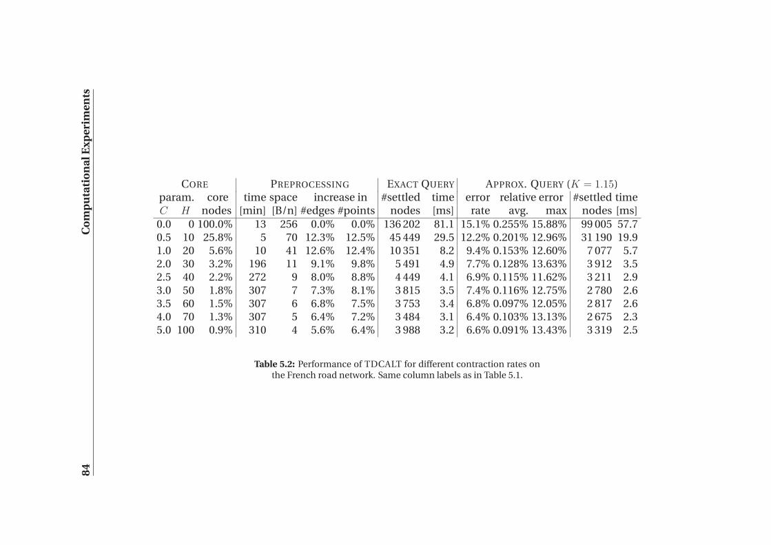
84
Co
mp
uta
tio
na
lE
xp
eri
me
nts
CORE PREPROCESSING EXACT QUERY APPROX. QUERY (K = 1.15)param. core time space increase in #settled time error relative error #settled timeC H nodes [min] [B/n] #edges #points nodes [ms] rate avg. max nodes [ms]
0.0 0 100.0% 13 256 0.0% 0.0% 136 202 81.1 15.1% 0.255% 15.88% 99 005 57.70.5 10 25.8% 5 70 12.3% 12.5% 45 449 29.5 12.2% 0.201% 12.96% 31 190 19.91.0 20 5.6% 10 41 12.6% 12.4% 10 351 8.2 9.4% 0.153% 12.60% 7 077 5.72.0 30 3.2% 196 11 9.1% 9.8% 5 491 4.9 7.7% 0.128% 13.63% 3 912 3.52.5 40 2.2% 272 9 8.0% 8.8% 4 449 4.1 6.9% 0.115% 11.62% 3 211 2.93.0 50 1.8% 307 7 7.3% 8.1% 3 815 3.5 7.4% 0.116% 12.75% 2 780 2.63.5 60 1.5% 307 6 6.8% 7.5% 3 753 3.4 6.8% 0.097% 12.05% 2 817 2.64.0 70 1.3% 307 5 6.4% 7.2% 3 484 3.1 6.4% 0.103% 13.13% 2 675 2.35.0 100 0.9% 310 4 5.6% 6.4% 3 988 3.2 6.6% 0.091% 13.43% 3 319 2.5
Table 5.2: Performance of TDCALT for different contraction rates onthe French road network. Same column labels as in Table 5.1.
5.3 Random Queries 85
one); as shortcuts represent optimal distances, the chance of computing a sub-optimal path decreases. Summarizing, large contraction parameters requiremore preprocessing time and space, but yield better results in terms of size ofthe search space and query speed. On the other hand, experiments on the dy-namic cost updates (Section 5.4) show that the length of shortcuts should belimited, if we want to perform cost updates in reasonable time.
Slightly different results are obtained on the French road network (Table 5.2).In this case, increasing contraction parameters always yields a decrease in re-quired preprocessing space. The reason for this is that time-dependent arcsare found only in one region of the graph (namely, Paris and its surroundings),and the number of arcs is relatively small. Therefore, for increasing C and Hwe essentially contract more static arcs, which have only one associated break-point (the static arc travelling time). This does not bring the explosion of thenumber of breakpoints, as observed on the European road network. As a con-sequence, required preprocessing space keeps decreasing. We can also see thatthe percentage of nodes in the core is typically smaller with respect to the Euro-pean road network with the same contraction parameters. We explain this byobserving that the limit on the maximum number of interpolation points thatwould appear on new shortcuts does not apply on this road network, becausethe number of interpolation points is small. Hence, more contraction is carriedout. The decrease in size of the search spaces and query times tails off afterC ≥ 2.5 and H ≥ 40. The same applies for error rate and relative error.
5.3 Random Queries
In this section we analyse the performance of TDCALT for different values ofthe approximation constant K, using the European road network as input. Inthis experiment we used contraction parameters C = 3.5 and H = 60, i.e. we al-low long shortcuts to be built so to favour query speed. We did not use larger val-ues for the contraction parameters because the reduction in terms of CPU timeis small, and the dynamic cost updates become unpractical (see Section 5.4).Results are recorded in Table 5.3 for the European road nework, and are gath-ered over 10 000 queries with source and destination nodes picked at random.For comparison, we also report the results on the same road network for thetime-dependent versions of Dijkstra, unidirectional ALT, TDALT and the time-dependent SHARC algorithm (Section 1.4.6). In particular, Dijkstra’s algorithmis used as a baseline to measure speedup factors, while SHARC currently rep-resents the state-of-the-art for time-dependent shortest paths algorithms, al-though it is not able to deal with dynamic scenarios. Results for the Frenchroad network are reported in Table 5.5.
We report the amount of preprocessing time (in minutes) and space (in ad-ditional bytes per node) required by each algorithm. Besides, the performed
86 Computational Experiments
queries may compute approximated results instead of optimal solutions, de-pending on the value of K; thus, as in Section 5.2 we record three differentstatistics to characterize the solution quality: error rate, average relative error,maximum relative error. We recall that error rate is the percentage of computedsuboptimal paths, and relative error on a particular query is the relative per-centage increase of the approximated solution over the optimum. We reportaverage and maximum values of the relative error over the set of all queries. Wealso record the average number of nodes settled at the end of the computationby each different algorithm, as well as the average CPU time in milliseconds.
In the following, we restrict ourselves to the scenario where only distances— not the complete paths — are required. However, our shortcut expansionroutine for TDCALT (Section 4.2.3) needs less than 1 ms to output the wholepath; the additional space overhead is≈ 4 bytes per node.
We focus on the European road network first, which is the largest instance,hence the most interesting. In terms of preprocessing space, TDCALT with con-traction parameters C = 3.5, H = 60 is the algorithm requiring less memory:only 61 additional bytes per node, while SHARC requires 118. Both TDALT andunidirectional ALT store landmark distances for all nodes in the graph, thusoccupying 256 additional bytes per node. Algorithms which do not employa hierarchical structure require a shorter preprocessing time: 28 minutes forTDALT and unidirectional ALT, which is the time to select 32 landmarks withthe avoid heuristic and compute landmark distances. The contraction phasetakes longer: 60 minutes for TDCALT, which only has to compute landmarkdistances for the core after the graph contraction, while SHARC takes 392 min-utes because of the computation of arc-flags.
We now analyse the size of the search spaces and query times for the differ-ent algorithms. We restrict our attention to exact algorithms, i.e. K = 1. In ourcomparison, the algorithm with the largest average search space is Dijkstra’s al-gorithm, with ≈ 8.8 millions nodes, and represents our baseline. The TDALTalgorithm yields a reduction of a factor 3 with respect to the baseline. Inter-estingly, unidirectional ALT settles 4.31 fewer nodes with respect to Dijkstra’salgorithm, thus it has a smaller search space than the bidirectional TDALT al-gorithm. This is easily explained if we consider that the bidirectional algorithmdescribed in Chapter 3 may explore twice all nodes in the search space of thebackward search. The SHARC algorithm only needs to settle 132.69 times fewernodes than Dijkstra’s algorithm, and TDCALT yields a further reduction, witha search space which is 145.76 smaller than the baseline. Thus, hierarchicalmethods are considerably more efficient in terms of number of settled nodeswith respect to algorithms that only deal with a plain graph, as confirmed bymany studies on static road networks (e.g. (19)).
If we consider the average number of settled nodes per millisecond, we ob-tain the following ranking:
1. Dijkstra’s algorithm: 1688.6
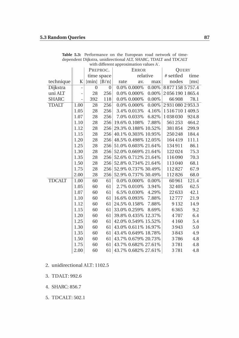
5.3 Random Queries 87
Table 5.3: Performance on the European road network of time-dependent Dijkstra, unidirectional ALT, SHARC, TDALT and TDCALT
with different approximation values K.
PREPROC. ERROR QUERY
time space relative # settled timetechnique K [min] [B/n] rate av. max nodes [ms]
Dijkstra - 0 0 0.0% 0.000% 0.00% 8 877 158 5 757.4uni ALT - 28 256 0.0% 0.000% 0.00% 2 056 190 1 865.4SHARC - 392 118 0.0% 0.000% 0.00% 66 908 78.1
TDALT 1.00 28 256 0.0% 0.000% 0.00% 2 931 080 2 953.31.05 28 256 3.4% 0.013% 4.16% 1 516 710 1 409.51.07 28 256 7.0% 0.033% 6.82% 1 038 030 924.81.10 28 256 19.6% 0.108% 7.88% 561 253 464.21.12 28 256 29.3% 0.188% 10.52% 381 854 299.91.15 28 256 40.1% 0.303% 10.95% 250 248 184.41.20 28 256 48.5% 0.498% 12.05% 164 419 111.11.25 28 256 51.0% 0.603% 21.64% 134 911 86.11.30 28 256 52.0% 0.669% 21.64% 122 024 75.31.35 28 256 52.6% 0.712% 21.64% 116 090 70.31.50 28 256 52.8% 0.734% 21.64% 113 040 68.11.75 28 256 52.9% 0.737% 30.49% 112 827 67.92.00 28 256 52.9% 0.737% 30.49% 112 826 68.0
TDCALT 1.00 60 61 0.0% 0.000% 0.00% 60 961 121.41.05 60 61 2.7% 0.010% 3.94% 32 405 62.51.07 60 61 6.5% 0.030% 4.29% 22 633 42.11.10 60 61 16.6% 0.093% 7.88% 12 777 21.91.12 60 61 24.5% 0.158% 7.88% 9 132 14.91.15 60 61 33.0% 0.259% 8.69% 6 365 9.21.20 60 61 39.8% 0.435% 12.37% 4 707 6.41.25 60 61 42.0% 0.549% 15.52% 4 160 5.41.30 60 61 43.0% 0.611% 16.97% 3 943 5.01.35 60 61 43.4% 0.649% 18.78% 3 843 4.91.50 60 61 43.7% 0.679% 20.73% 3 786 4.81.75 60 61 43.7% 0.682% 27.61% 3 781 4.82.00 60 61 43.7% 0.682% 27.61% 3 781 4.8
2. unidirectional ALT: 1102.5
3. TDALT: 992.6
4. SHARC: 856.7
5. TDCALT: 502.1
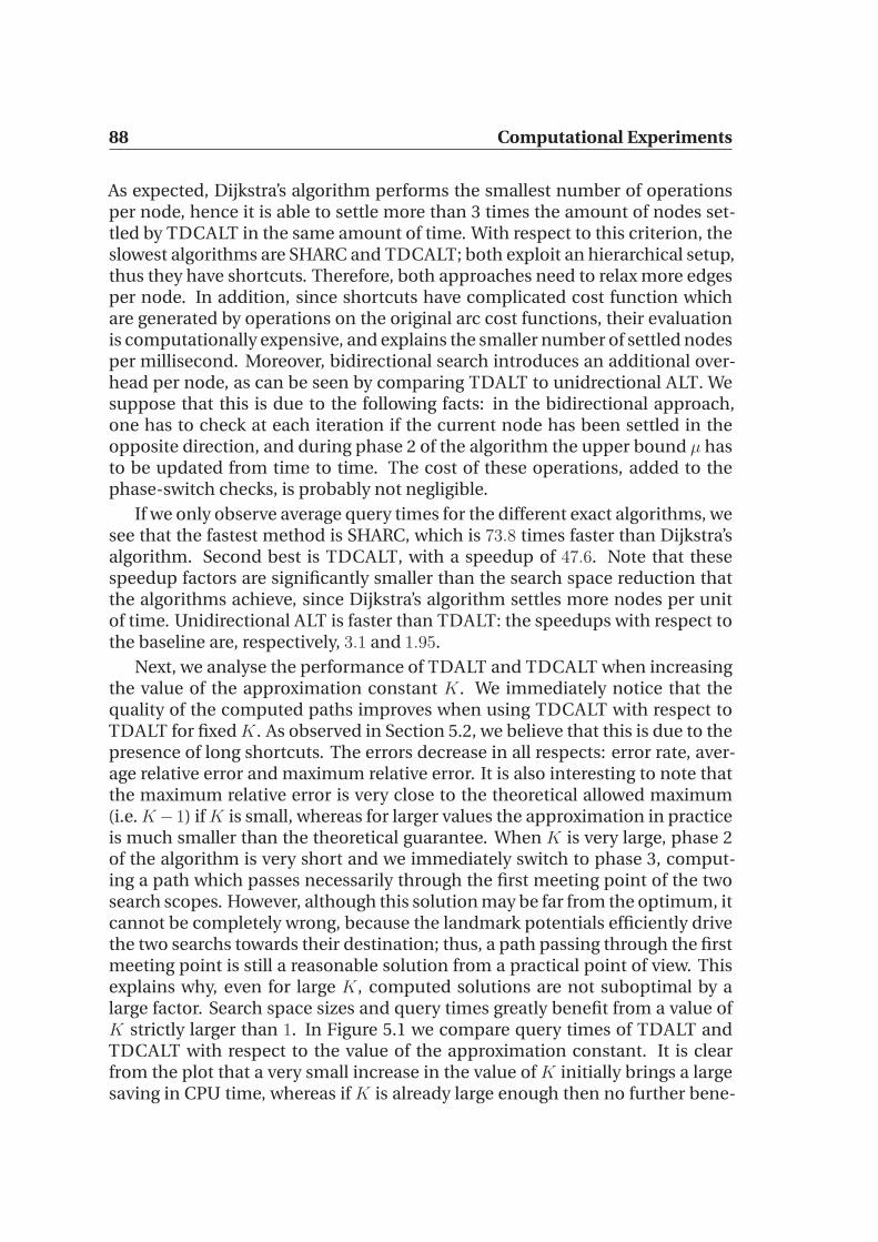
88 Computational Experiments
As expected, Dijkstra’s algorithm performs the smallest number of operationsper node, hence it is able to settle more than 3 times the amount of nodes set-tled by TDCALT in the same amount of time. With respect to this criterion, theslowest algorithms are SHARC and TDCALT; both exploit an hierarchical setup,thus they have shortcuts. Therefore, both approaches need to relax more edgesper node. In addition, since shortcuts have complicated cost function whichare generated by operations on the original arc cost functions, their evaluationis computationally expensive, and explains the smaller number of settled nodesper millisecond. Moreover, bidirectional search introduces an additional over-head per node, as can be seen by comparing TDALT to unidrectional ALT. Wesuppose that this is due to the following facts: in the bidirectional approach,one has to check at each iteration if the current node has been settled in theopposite direction, and during phase 2 of the algorithm the upper bound µ hasto be updated from time to time. The cost of these operations, added to thephase-switch checks, is probably not negligible.
If we only observe average query times for the different exact algorithms, wesee that the fastest method is SHARC, which is 73.8 times faster than Dijkstra’salgorithm. Second best is TDCALT, with a speedup of 47.6. Note that thesespeedup factors are significantly smaller than the search space reduction thatthe algorithms achieve, since Dijkstra’s algorithm settles more nodes per unitof time. Unidirectional ALT is faster than TDALT: the speedups with respect tothe baseline are, respectively, 3.1 and 1.95.
Next, we analyse the performance of TDALT and TDCALT when increasingthe value of the approximation constant K. We immediately notice that thequality of the computed paths improves when using TDCALT with respect toTDALT for fixed K. As observed in Section 5.2, we believe that this is due to thepresence of long shortcuts. The errors decrease in all respects: error rate, aver-age relative error and maximum relative error. It is also interesting to note thatthe maximum relative error is very close to the theoretical allowed maximum(i.e. K− 1) if K is small, whereas for larger values the approximation in practiceis much smaller than the theoretical guarantee. When K is very large, phase 2of the algorithm is very short and we immediately switch to phase 3, comput-ing a path which passes necessarily through the first meeting point of the twosearch scopes. However, although this solution may be far from the optimum, itcannot be completely wrong, because the landmark potentials efficiently drivethe two searchs towards their destination; thus, a path passing through the firstmeeting point is still a reasonable solution from a practical point of view. Thisexplains why, even for large K, computed solutions are not suboptimal by alarge factor. Search space sizes and query times greatly benefit from a value ofK strictly larger than 1. In Figure 5.1 we compare query times of TDALT andTDCALT with respect to the value of the approximation constant. It is clearfrom the plot that a very small increase in the value of K initially brings a largesaving in CPU time, whereas if K is already large enough then no further bene-
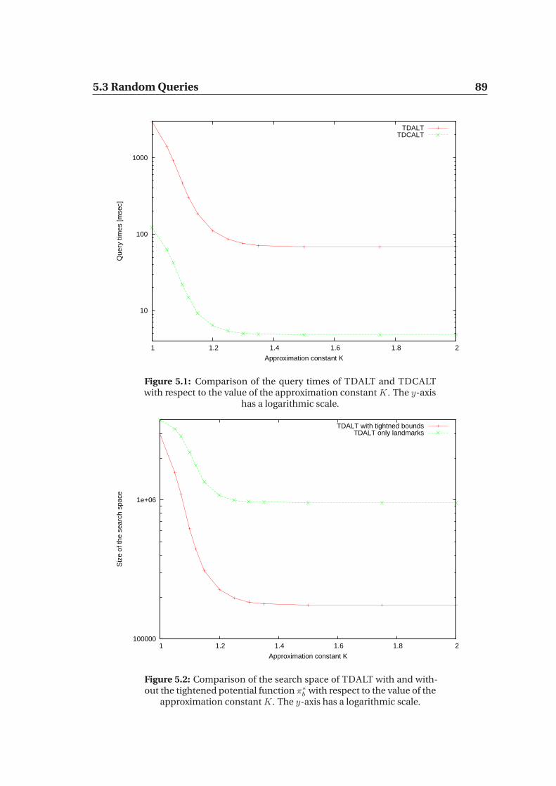
5.3 Random Queries 89
10
100
1000
1 1.2 1.4 1.6 1.8 2
Que
ry ti
mes
[mse
c]
Approximation constant K
TDALTTDCALT
Figure 5.1: Comparison of the query times of TDALT and TDCALTwith respect to the value of the approximation constant K. The y-axis
has a logarithmic scale.
100000
1e+06
1 1.2 1.4 1.6 1.8 2
Siz
e of
the
sear
ch s
pace
Approximation constant K
TDALT with tightned boundsTDALT only landmarks
Figure 5.2: Comparison of the search space of TDALT with and with-out the tightened potential function π∗
bwith respect to the value of the
approximation constant K. The y-axis has a logarithmic scale.
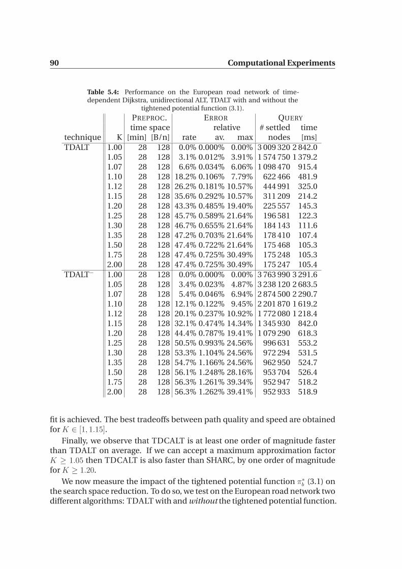
90 Computational Experiments
Table 5.4: Performance on the European road network of time-dependent Dijkstra, unidirectional ALT, TDALT with and without the
tightened potential function (3.1).
PREPROC. ERROR QUERY
time space relative # settled timetechnique K [min] [B/n] rate av. max nodes [ms]
TDALT 1.00 28 128 0.0% 0.000% 0.00% 3 009 320 2 842.01.05 28 128 3.1% 0.012% 3.91% 1 574 750 1 379.21.07 28 128 6.6% 0.034% 6.06% 1 098 470 915.41.10 28 128 18.2% 0.106% 7.79% 622 466 481.91.12 28 128 26.2% 0.181% 10.57% 444 991 325.01.15 28 128 35.6% 0.292% 10.57% 311 209 214.21.20 28 128 43.3% 0.485% 19.40% 225 557 145.31.25 28 128 45.7% 0.589% 21.64% 196 581 122.31.30 28 128 46.7% 0.655% 21.64% 184 143 111.61.35 28 128 47.2% 0.703% 21.64% 178 410 107.41.50 28 128 47.4% 0.722% 21.64% 175 468 105.31.75 28 128 47.4% 0.725% 30.49% 175 248 105.32.00 28 128 47.4% 0.725% 30.49% 175 247 105.4
TDALT− 1.00 28 128 0.0% 0.000% 0.00% 3 763 990 3 291.61.05 28 128 3.4% 0.023% 4.87% 3 238 120 2 683.51.07 28 128 5.4% 0.046% 6.94% 2 874 500 2 290.71.10 28 128 12.1% 0.122% 9.45% 2 201 870 1 619.21.12 28 128 20.1% 0.237% 10.92% 1 772 080 1 218.41.15 28 128 32.1% 0.474% 14.34% 1 345 930 842.01.20 28 128 44.4% 0.787% 19.41% 1 079 290 618.31.25 28 128 50.5% 0.993% 24.56% 996 631 553.21.30 28 128 53.3% 1.104% 24.56% 972 294 531.51.35 28 128 54.7% 1.166% 24.56% 962 950 524.71.50 28 128 56.1% 1.248% 28.16% 953 704 526.41.75 28 128 56.3% 1.261% 39.34% 952 947 518.22.00 28 128 56.3% 1.262% 39.41% 952 933 518.9
fit is achieved. The best tradeoffs between path quality and speed are obtainedfor K ∈ [1, 1.15].
Finally, we observe that TDCALT is at least one order of magnitude fasterthan TDALT on average. If we can accept a maximum approximation factorK ≥ 1.05 then TDCALT is also faster than SHARC, by one order of magnitudefor K ≥ 1.20.
We now measure the impact of the tightened potential function π∗b (3.1) onthe search space reduction. To do so, we test on the European road network twodifferent algorithms: TDALT with and without the tightened potential function.

5.3 Random Queries 91
Therefore, the latter will only use the landmark potential functions; we call thisalgorithm TDALT−. In this setup, we used 16 landmarks generated with themaxCover heuristic (70). Results are reported in Table 5.4.
We observe that the tightened potential function reduces both the size of thesearch space and query times by a large factor. For exact queries, the averagenumber of settled nodes is reduced by a factor 1.25, and query times by a factor1.16. As we increase K, the impact of the π∗b rapidly becomes larger: for K = 1.1,the search space reduction is of a factor 3.53, 4.39 for K = 1.15, up to a maxi-mum of 5.43 for K = 1.5 and above. Figure 5.2 plots the size of the search spaceof TDALT and TDALT− with respect to the value of K, and supports our anal-ysis. A similar behaviour is observed for query times. Moreover, the error ratedecreases when using the tightened potential function, as well as both averageand maximum error rate. This is not a trivial result: since TDCALT− explores asignificantly larger amount of nodes, one would expect that it would find bettersolutions. This observation leads us to think that the tightened potential func-tion not only reduces the number of settled nodes in general, but also prunesthe search at nodes which cannot appear on good solutions, therefore yieldinga more efficient exploration of the graph.
We now consider results obtained on the French road network, and reportedin Table 5.5. We note that all reported values are subject to very small changes,if any at all, for K ≥ 1.10. We give the following explanation: since the ma-jority of arcs in this instance is static, the cost lower bounds given by λ whichare used to compute landmark distances are equal to the costs used throughthe shortest paths computations, leading to near-optimal performance of land-mark potentials. Therefore, there is not much room for improvement in termsof size of the search space. The only value which is affected by large values ofK is the maximum relative error: the search stops sooner by a small amount ofnodes, as indicated by the average size of the search space, but the maximumerror increases by significant amounts. This suggests that important nodes aresometimes skipped during the search. Overall, it does not seem profitable inpractice to set K ≥ 1.10.
In terms of query speed, Unidirectional ALT is one order of magnitude fasterthan Dijkstra’s algorithm. TDALT yields an additional CPU time saving of afactor two. TDCALT is on average one order of magnitude faster than TDALT,therefore almost three orders of magnitude faster than Dijkstra’s algorithm. Sim-ilar considerations can be done with respect to the size of the search spaces.Error related values also decrease when switching from TDALT to TDCALT, asobserved on the European instance. Summarizing, the analysis carried out onthe road network of Western Europe is also valid for the road network of France,with the exception of the different behaviour of preprocessing time and space –which is discussed in Section 5.2.

92 Computational Experiments
Table 5.5: Performance on the French road network of time-dependent Dijkstra, unidirectional ALT, TDALT and TDCALT with dif-
ferent approximation values K.
PREPROC. ERROR QUERY
time space relative # settled timetechnique K [min] [B/n] rate av. max nodes [ms]
Dijkstra - 0 0 0.0% 0.000% 0.00% 3 615 670 1 723.4uni ALT - 13 256 0.0% 0.000% 0.00% 290 178 140.5
TDALT 1.00 13 256 0.0% 0.000% 0.00% 136 202 81.41.05 13 256 14.1% 0.166% 4.96% 100 884 59.01.07 13 256 14.6% 0.205% 7.00% 100 013 58.41.10 13 256 15.0% 0.234% 9.89% 99 303 58.01.12 13 256 15.0% 0.243% 12.00% 99 156 57.91.15 13 256 15.1% 0.255% 14.02% 99 062 57.81.50 13 256 15.2% 0.260% 32.44% 98 970 57.72.00 13 256 15.2% 0.260% 32.44% 98 969 57.7
TDCALT 1.00 307 6 0.0% 0.000% 0.00% 3 790 3.51.05 307 6 6.0% 0.064% 4.89% 2 876 2.61.07 307 6 6.5% 0.085% 6.36% 2 848 2.61.10 307 6 6.8% 0.107% 9.55% 2 832 2.51.12 307 6 6.9% 0.114% 10.07% 2 830 2.51.15 307 6 7.0% 0.119% 12.43% 2 828 2.51.50 307 6 7.1% 0.122% 16.62% 2 826 2.52.00 307 6 7.1% 0.122% 16.62% 2 826 2.5
5.3.1 Local Queries
For random queries, TDCALT is one order of magnitude faster than TDALT onaverage. TDCALT is significantly faster than unidirectional ALT, while TDALTis faster than the unidirectional version of the algorithm only for K ≥ 1.05. Inorder to gain insight whether these speedups derive from small or large dis-tance queries, Fig. 5.3 reports the query times with respect to the Dijkstra rank,obtained on the European road network. For an s-t query, the Dijkstra rank ofnode t is the number of nodes settled before t is settled: thus, it is some kind ofdistance measure. These values were gathered on the European road networkinstance, using contraction parameters as in Table 5.3, i.e. c = 3.5 and h = 60.
Note that we use a logarithmic scale due to the fluctuating query times. Thefigure clearly indicates that both speedup techniques pay off only for long dis-tance queries. If the source and destination node are close to each other, thenunidirectional ALT is faster than TDCALT by an order of magnitude in somecases. This is expected, since for small distances TDCALT may result in a sim-ple application of Dijkstra’s algorithm, with no speedup techniques. For suffi-ciently long distances, however, the median of TDCALT is almost two orders
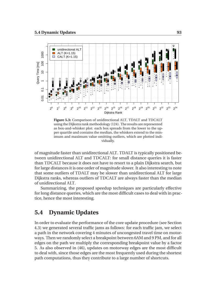
5.4 Dynamic Updates 93
Dijkstra Rank
Que
ry T
ime
[ms]
26 27 28 29 210 211 212 213 214 215 216 217 218 219 220 221 222 223 224
0.01
0.1
110
100
1000
unidirectional ALTALT (K=1.15)CALT (K=1.15)
Figure 5.3: Comparison of unidirectional ALT, TDALT and TDCALTusing the Dijkstra rank methodology (124). The results are representedas box-and-whisker plot: each box spreads from the lower to the up-per quartile and contains the median, the whiskers extend to the min-imum and maximum value omitting outliers, which are plotted indi-
vidually.
of magnitude faster than unidirectional ALT. TDALT is typically positioned be-tween unidirectional ALT and TDCALT: for small distance queries it is fasterthan TDCALT because it does not have to resort to a plain Dijkstra search, butfor large distances it is one order of magnitude slower. It also interesting to notethat some outliers of TDALT may be slower than unidirectional ALT for largeDijkstra ranks, whereas outliers of TDCALT are always faster than the medianof unidirectional ALT.
Summarizing, the proposed speedup techniques are particularly effectivefor long distance queries, which are the most difficult cases to deal with in prac-tice, hence the most interesting.
5.4 Dynamic Updates
In order to evaluate the performance of the core update procedure (see Section4.3) we generated several traffic jams as follows: for each traffic jam, we selecta path in the network covering 4 minutes of uncongested travel time on motor-ways. Then we randomly select a breakpoint between 6AM and 9 PM, and for alledges on the path we multiply the corresponding breakpoint value by a factor5. As also observed in (46), updates on motorway edges are the most difficultto deal with, since those edges are the most frequently used during the shortestpath computations, thus they contribute to a large number of shortcuts.

94
Co
mp
uta
tio
na
lE
xp
eri
me
nts
traffic jam single breakpointcont. limit space single[ms] batch[ms] single[ms] batch[ms] queryC H [min] [B/n] av. max av. max av. max av. max [ms]
0.0 0 – 256 0.0 0 0 0 0.0 0 0 0 188.2
0.5 10 5 123 0.4 28 372 488 0.1 5 97 166 81.510 121 0.7 49 619 799 0.1 12 183 383 85.215 119 0.7 49 707 1 083 0.1 11 202 407 74.220 119 0.7 49 820 1 200 0.2 59 291 459 73.8
1.0 20 5 82 7.8 229 7 144 8 090 1.8 78 1 853 2 041 34.510 72 21.2 778 20 329 22 734 5.8 371 5 957 9 266 27.115 68 32.1 2 226 27 327 33 313 7.2 427 7 291 11 522 25.420 66 37.0 2 231 30 787 39 470 8.8 1 197 8 476 11 426 22.8
2.0 30 5 88 17.4 290 16 293 17 493 5.7 283 5 019 6 017 33.710 82 90.5 3 868 79 092 85 259 27.6 1 894 24 943 27 501 22.815 79 171.0 4 604 120 018 142 455 49.4 2 451 46 237 58 936 19.720 77 219.7 5 073 187 595 206 569 63.3 5 510 60 940 65 954 16.4
Table 5.6: CPU time required to update the core for different contrac-tion parameters and limits for the length of shortcuts.

5.4 Dynamic Updates 95
In Table 5.6 we report average and maximum required time over 1000 runsto update the core in case of a single traffic jam, applying different contrac-tion parameters. We also report the corresponding figures for a batch update of1000 traffic jams (computed over 100 runs), in order to reduce the fluctuationsand give a clearer indication of required CPU time when performing multipleupdates. Besides, we measured the average and maximum time required to up-date the core when modifying a single breakpoint on a motorway arc selecteduniformly at random; we also record the corresponding values when modifying1000 single breakpoints on random motorway arcs (computed over 100 runs).As there is no spatial locality when updating a single breakpoint over randomarcs, this represents a worst-case scenario. Note that in this experiment welimit the length of shortcuts in terms of uncongested travel time (as reportedin the third column). This is because in the dynamic scenario the length ofshortcuts plays the most important role when determining the required CPUeffort for an update operation, and if we allow the shortcuts length to grow in-definitely we may have unpractical update times. Hence, we also report pre-processing space in terms of additional bytes per node, and query times withK = 1.15. We remark that Table 5.6 only considers the CPU time required toupdate the core, and does not take into account the computational effort tomodify the cost functions for arcs at level 0 in the hierarchy, i.e. not belongingto the core. However, this effort is negligible in practice, because the modifi-cation of a breakpoint of an arc outside the core has an influence only on thearc itself. Therefore, the update is carried out by simply modifying the corre-sponding breakpoint value, whereas the core update is considerably more time-consuming (see Section 4.3).
As expected, the effort to update the core becomes more expensive withincreasing contraction parameters. First, we consider the scenario where wegenerate 1000 traffic jams over motorway arcs, and modify the cost functionsaccordingly. For C = 0.5, H = 10 the updates are very fast, even if we allow longshortcuts (i.e. 20 minutes of uncongested travel time). The average CPU timefor an update of 1000 traffic jams is always smaller than 1 second, thereforewe are able to deal with a large number of breakpoint modifications in a shorttime. This is confirmed by the very small average time required to update thecore after modifying a random breakpoint on a random motorway arc, whichis smaller than 0.2 milliseconds. As we increase the contraction parameters, dy-namic updates take longer to deal with. A larger number of long shortcuts iscreated, therefore update times grow rapidly, requiring several seconds. Theaverage time to update the core after adding 1000 traffic jams with contractionparameters C = 1, H = 20 is at least one order of magnitude larger than the re-spective values with parameters C = 0.5, H = 10. Very large updates are feasiblein practice only if we limit the length of shortcuts to 5 minutes of uncongestedtravel time; for most practical applications, however, updates are not very fre-quent, therefore adding 1000 traffic jams in ≈ 30 seconds is reasonably fast. If

96 Computational Experiments
we consider contraction parameters C = 2, H = 30, then the updates for thisscenario may require several minutes; however, limiting the length of shortcutshelps.
Next, we analyse update times for modifications of a single breakpoint overrandom motorway arcs. We observe that they confirm the analysis for the pre-vious scenario (adding 1000 traffic jams). For small contraction parameters (orif we limit shortcuts to a small length in terms of uncongested travelling time),updating the core after modifying one breakpoint requires on average less than10 milliseconds, whereas if we modify 1000 breakpoints we need less than 10seconds. For C = 0.5, H = 10 we can carry out the updates in less than 0.5 sec-onds. If we allow shortcuts to grow, then updates may require several seconds.
If we compare the time required to update the core after adding 1000 trafficjams with respect to modifying 1000 breakpoints, we see that our update rou-tine greatly benefits from spatial locality of the modified arcs: the first scenariois only ≈3-4 times slower than the second, but the number of modified arcs islarger, because each traffic jam extends over several motorway arcs. However,this is expected: as each shortcut is updated only once, modifications on con-tiguous arcs may require no additional effort, if all modified arcs belong to thesame shortcut. In real world applications, traffic jams typically occur on con-tiguous arcs (86), therefore our update routine should behave better in practicethan in worst case scenarios.
Summarizing, we observe a clear trade off between query times and updatetimes depending on the contraction parameters, so that for those applicationswhich require frequent updates we can minimize update costs while keepingquery times < 100 ms, and for applications which require very few or no up-dates we can minimize query times. If most of the arcs have their cost changedwe can rerun the core arcs computation, i.e. recomputing all arcs on the corefrom scratch, which only takes a few minutes.

Chapter 6
A Real-World Application
One of the main objective of this thesis was to develop an algorithm capableof answering several shortest path queries per second, so that a real-time pathcomputing service taking into account both real-time traffic and traffic fore-castings could be proposed on the website of the Mediamobile company. Inthis section we describe the existing industrial platform of this company, andthe architecture of a new platform which integrates the algorithm describedabove with the existing components.
The rest of this section is organized as follows. In Section 6.1 we briefly de-scribe the existing components in the architecture where we wish to integrateour implementation of the TDCALT algorithm. In Section 6.2 we give a de-scription of how this integration was carried out. In Section 6.3 we give a math-ematical formulation for the problem of computing the updated cost functionbreakpoint values, so as to adapt the function to real-time traffic informationand forecastings.
6.1 Description of the existing architecture
Mediamobile is a company whose primary purpose is to gather, aggregate andredistribute real-time traffic information. Several services are built on top ofthis basic function. The main component of their architecture is the traffic in-formation server SDT (Serveur De Trafic, “traffic server” in French), which gath-ers real-time traffic information from various sources and treats them so as tomake them directly utilizable for other services. In particular, the SDT is alsothe provider of traffic forecast information, and, as such, is the only source oftraffic information which is necessary for our needs.
Real-time traffic information is obtained through different means: the mostreliable information is measured directly on-site by local administrations, usu-ally by means of electromagnetic loops or cams that are capable of determiningthe speed of passing vehicles. Another important source is represented by Float-

98 A Real-World Application
ing Car Data: cars driving in a fleet are equipped with GPS devices that con-stantly monitor their position and speed, therefore providing information onthe congestion status of road segments that some vehicles have recently gonethrough. Real-time traffic information is updated every few minutes (tipically,two minutes). Real-time traffic information is then used to feed different pre-diction models, so that traffic forecasts are generated. Forecasts are dividedinto three different categories, depending on the time horizon after the predic-tion is made that they address:
1. short-term forecasts: a few seconds to 10-20 minutes,
2. mid-term forecasts: 10-20 minutes to 4-5 hours,
3. long-term forecasts: 4-5 hours to several months.
Long-term forecasts rest on aggregated historical data, and represent the speedprofiles which were referred to throughout this thesis. Short- and mid-termforecasts are updated every few minutes, as a consequence of changes in thereal-time traffic information, whereas long-term forecasts may be updated onceevery several months or even years, thus they can be considered as static infor-mation.
The SDT provides an API that allows other services to query and obtain traf-fic information; among these services, the one that is relevant for this thesis isthe one that provides the main features of the site www.v-trafic.com, which al-lows web users to see the real-time traffic status over all France. This serviceruns on a Windows machine and exposes a web service towards the web site.In the following, we will refer to the C# application run by this machine as thepaths computation service. A screenshot of the web site with the route planningmodule can be found in Figure 6.1. Note that, at the moment of writing this the-sis, the only front-end for the integrated path computation platform describedin this section is the web site, but it would be easy to allow any device with in-ternet connection capabilities to query the platform. In particular, this couldbe implemented for GPS devices, so as to allow an internet-connected servicewhere the GPS need not know real-time traffic information and forecasts overthe whole network: it suffices to send a path query to the path computationplatform, which utilizes all the available traffic information up-to-date, and dis-play the path which answers the query. Our objective is to integrate our C++implementation of TDCALT with the C# paths computation service, so as toprovide users with the possibility of calculating the optimal path between twopoints. The paths computation service has an internal graph representation ofthe French road network, since it must be able to project points on the roadnetwork (i.e. find the node which is closer to given cohordinates) and draw onthe map, in order to indicate the traffic congestion status on monitored roadsegments and highlight the computed path after a shortest path query. Thesecapabilities are implemented using the Google Maps API (73). Moreover, this
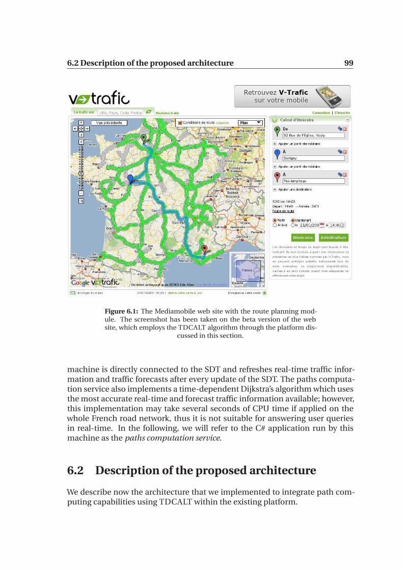
6.2 Description of the proposed architecture 99
Figure 6.1: The Mediamobile web site with the route planning mod-ule. The screenshot has been taken on the beta version of the website, which employs the TDCALT algorithm through the platform dis-
cussed in this section.
machine is directly connected to the SDT and refreshes real-time traffic infor-mation and traffic forecasts after every update of the SDT. The paths computa-tion service also implements a time-dependent Dijkstra’s algorithm which usesthe most accurate real-time and forecast traffic information available; however,this implementation may take several seconds of CPU time if applied on thewhole French road network, thus it is not suitable for answering user queriesin real-time. In the following, we will refer to the C# application run by thismachine as the paths computation service.
6.2 Description of the proposed architecture
We describe now the architecture that we implemented to integrate path com-puting capabilities using TDCALT within the existing platform.

100 A Real-World Application
Internet
Internet
Floating Car Data Electromagnetic rings
Cams
Pathcomputationweb service
Traffic
TDCALTserver
Sourcesof trafficinformation
informationserver(SDT)
Figure 6.2: Schematic representation of the proposed architecture.
One of the first difficulties that we had to deal with is the fact that the exist-ing paths computation service is coded in C# and runs on Windows, whereasour TDCALT implementation is coded in C++ and runs on Linux. Thus, bothapplications could not run on the same machine. We decided to run the TD-CALT implementation on a separate machine, which is only accessible throughthe paths computation service, and whose only purpose is to compute the pathsbetween two points with starting time at a given time of the day. A sketch of thisarchitecture can be seen in Figure 6.2.
The TDCALT server has an internal graph representation which uses differ-ent node and arc identifiers; the reason behind this is that identifiers provided

6.2 Description of the proposed architecture 101
by mapping companies (e.g. NavTeq, TeleAtlas) are typically unpractical to dealwith, due to excessive length, whereas our C++ implementation needs integeridentifiers for both arc and nodes which are contiguous and start from zero.Thus, we compute a mapping between the graph representation available onthe paths computation service and the one used by the TDCALT server. Thepaths computation service in C# is responsible for the following tasks:
• expose a web service towards the web site;
• obtain the updated traffic information from the SDT, process it and sendit to the TDCALT server;
• translate external arc/node identifiers into the identifiers used by the TD-CALT server, and vice-versa;
• manage the queue of pending queries;
• compute and display the road map on the web site after a path has beencomputed.
The processing of updated traffic information, i.e. the update of the coefficientsof the piecewise linear cost functions, is described in more detail in Section 6.3.Communication towards and from the TDCALT server is carried out throughTCP/IP with binary encoded messages.
The TDCALT server accepts incoming TCP packets on two different ports.The first one is dedicated to the computation of shortest paths: a query packetcontains the internal identifier of the source and destination nodes, as trans-lated by the C# paths computation service through the available mapping, andthe departure time; the machine carries out the calculations, and returns backthe list of arcs on the shortest path, as well as its cost. Shortest paths compu-tations cannot be done in parallel, since the nodes are labeled with one of thedifferent statuses: unreached, explored, settled (see Section 1.4.2), and foreach query the labels must be initialized. The second port is dedicated to thecost function updates. Whenever the cost function should be updated, the C#service sends to the TDCALT server the data containing arc identifiers and newbreakpoint values through this port. When an update is pending, the TDCALTserver does not accept path queries anymore; if there is a shortest path compu-tation in progress, then that computation is carried out. As soon as there are nopath computations in progress, the update phase starts: the set of all shortcutsthat must be updated is split equally among all available CPUs, and the proce-dure discussed in Section 4.3 is applied. Since each shortcut can be updatedindependently from the others, this routine can be run in parallel with no addi-tional effort. When the update procedure is complete, the path computationsresume normally.
102 A Real-World Application
Additionally, we run an instance of the TDCALT server without real-timetraffic information. This serves the purpose of answering shortest paths querieswhose departure time is not in the near future with respect to the instant atwhich the query is received. Typically, this happens when users want to com-pute a shortest route using statistical information for a particular day of theweek. To this end, Mediamobile provides 4 different speed profiles, that cor-respond to different combinations between subsets of days in the week andholiday/working day. We run an instance of the TDCALT which manages all 4profiles, and answers to shortest paths queries using the most appropriate one.
The TDCALT server is run on a machine equipped with a Quad-Core AMDOpteron 2354 processor and 16 GB of RAM. Summarizing, this machine runsan instance of the server with real-time traffic information on one core, and aninstance without real-time traffic information and 4 different speed profiles onanother core; as these instances are run separately, they can be used in parallel.The first instance takes approximately 1.6 GB of RAM, the second one 4 GB. Thetwo remaining CPU cores are used only for the profile update.
6.2.1 Load balancing and fault tolerance
We implemented a simple fault tolerance scheme to increase the availability ofthe path computation service. At the same time, this scheme provides a loadbalancing mechanism. The scheme is illustrated in Figure 6.3, and works as fol-lows. Both the machine that runs the C# path computation service and the C++TDCALT server are duplicated, so that there are two perfectly equal platformsto answer a shortest path query. A load balancer is put in the layer betweenusers (e.g. the website) and the C# path computation service, and dispatchesrequests to the machine with the smallest work load. Similarly, a load balancerrepresents the layer between the two machines that run che C# path computa-tion service and the C++ TDCALT server. Requests are dispatched to the firstavailable machine. The two load balancers also implement a fault tolerancescheme: whenever one of the queried machines is down, queries are automati-cally sent to its duplicate. All messages are exchanged as short TCP packets andeach TCP connection is valid for one shortest path query only; therefore, theload balancer can connect a C# path computation service to a C++ TDCALTserver by simply forwarding the TCP packet containing the query. Note that, interms of performance, it would be better to keep the connection between theC# path computation server and the TDCALT server always open, so that wedo not have to waste resources on establishing the connection. However, withsuch a scheme we would not be able to implement the fault tolerance and loadbalancing mechanism.
It can be seen that this architecture provides a natural way to deal with real-time traffic information updates: whenever one of the two real-time TDCALTservers is running an update (and is therefore unvailable for shortest paths com-

6.2 Description of the proposed architecture 103
Internet
Pathcomputationweb service
Loadbalancer
Loadbalancer
TDCALTserver
Figure 6.3: Schematic representation of the load balancing and faulttolerance scheme.
putations), the load balancer forwards all queries to the duplicate machine,which will update the profiles only when the first one has finished the update.This way, at least one of the two machines is always available.
The load balancer is able to tell the status of each TDCALT server by query-ing a monitoring service via TCP. The monitoring service is a thread spawned bythe main TDCALT process, which therefore shares the same address space andis able to detect if the main program has encountered errors. The monitoringthread listens for TCP connection on a different port than the main TDCALTprocess, and, whenever it receives a message, sends back one of the followingtwo-characters ASCII encoded strings:
1. OK: the server is alive and working;
2. KO: the server is alive but has encountered problem that prevent it fromanswering to queries (e.g. network related problems);
3. UP: the server is alive but is currently updating profiles.

104 A Real-World Application
Obviously, if the monitoring thread does not answer or does not accept the con-nection, the main TDCALT process is considered to be dead or unreachable.Since the load balancer queries the TDCALT server status every second, it maytake up to one second to propagate the status information to the load balancer.Therefore, when a TDCALT server wants to perform an update of its cost func-tions, it first sets its status to UP, then waits for one second (while still acceptingand answering incoming path queries), and finally starts the update. This waywe avoid sending shortest path queries to a TDCALT server which is perform-ing an update.
6.3 Updating the cost function coefficients
Through this section, we assume that for each time instant there is no overlap-ping traffic information, i.e. we only have one of the following:
1. real-time information,
2. short-term forecasts,
3. mid-term forecasts,
4. long-term forecasts,
taken in order of accuracy. For a given arc, each information is representedas point (τ, f(τ)) where τ represents the time instant and f(τ) is the travellingtime over that arc starting the traversal at time τ . Whenever one of the differentsources of traffic information is updated, we would like to compute the piece-wise linear function that best fits the new information, so that the correspond-ing arc cost function can be updated. Since this task must be carried out often,it should have a small computational cost. Hence, it is natural to solve this prob-lem using a least squares estimation of the cost function. We state the problemformally as follows.
We are given a set of points (xi, yi), i = 1, . . . , n where xi ∈ [0, P ] ∀i = 1, . . . , nand a set of breakpoint positions r1 = 0, . . . , rm+1 = P with ri ∈ [0, P ] ∀i =1, . . . ,m + 1 such that [0, P ] can be partitioned into m intervals [ri, ri+1] i = 1, . . . ,m.We want to compute a continuous piecewise linear function f : [0, P ]→ R,
f(x) = aix + bi if x ∈ [ri, ri+1), (6.1)
periodic of period P , that minimizes the sum of the quadratic errors:
∆ =n
∑
i=1
(f(xi)− yi)2. (6.2)

6.3 Updating the cost function coefficients 105
In order for f to be continuous, the condition
airi+1 + bi = ai+1ri+1 + bi+1 (6.3)
must hold ∀i = 1, . . . ,m− 1; since f is periodic, we also have
b1 = amrm+1 + bm. (6.4)
Constraints (6.3) allow us to express bi for i = 2, . . . ,m in terms of the remainingvariables, while (6.4) expresses am in terms of b1 and bm. With simple algebraiccalculations we obtain
bi =i
∑
j=2
(aj + aj−1)rj + b1 ∀i = 2, . . . ,m, (6.5)
and
am = −
∑m
j=2(aj + aj−1)rj
P. (6.6)
Thus, we need to optimize over the m variables b1, a1, . . . , am−1. This is a convexproblem which can be solved by vanishing the derivatives of (6.2) with respectto the variables. We obtain:
d∆
db1
=∑
xj∈[0,r2]
(a1xj + b1 − yj) +m
∑
i=2
∑
xj∈[ri,ri+1]
(aixj +i
∑
h=2
(ah + ah−1)rh + b1 − yj)
d∆
da1
=∑
xj∈[r1,r2]
(a1xj + b1 − yj)xj +
+m
∑
i=2
∑
xj∈[ri,ri+1]
(aixj +i
∑
h=2
(ah + ah−1)rh + b1 − yj)(r2 + r1)
...
d∆
dak
=∑
xj∈[rk,rk+1]
(akxj +k
∑
h=2
(ah + ah−1)rh + b1 − yj)xj +
+m
∑
i=k+1
∑
xj∈[ri,ri+1]
(aixj +i
∑
h=2
(ah + ah−1)rh + b1 − yj)(rk+1 + rk)
...
d∆
dam−1
=∑
xj∈[rm−1,rm]
(am−1xj +m−1∑
h=2
(ah + ah−1)rh + b1 − yj)xj +
+∑
xj∈[rm,P ]
(−
∑m
h=2(ah + ah−1)rh
Pxj +
m∑
h=2
(ah + ah−1)rh + b1 − yj)(P + rm−1).

106 A Real-World Application
Solving this m×m linear system yields the optimal coefficients ai, bi i = 1, . . . ,m,which define the updated cost function (6.1).
Not all coefficients ai, bi i = 1, . . . ,m must be modified at each update step.The main purpose of this procedure is to take into account real-time traffic in-formation and forecasts in order to provide a reliable path to those users whichare interested in computing a path with departure time close to the time instantat which the path is queried (via the web service). Obviously, it does not makesense to request paths with departure time in the past. Thus, we only updatecoefficients “in the future” with respect to the time at which the update is made.Formally, we are given a set of points (xi, yi), i = 1, . . . , n such that (f(xi) −yi)/f(xi) ≥ T , where T is a given threshold; this means that the current piece-wise linear function f(x) does not fit the points (xi, yi), i = 1, . . . , n, hence weneed to update its coefficients. Let [rL, rU ] be an interval with endpoints definedas: L = arg maxj∈{1,...,m+1}{rj|rj ≤ xi, i = 1, . . . , n}, U = arg minj∈{1,...,m+1}{rj|rj ≥xi, i = 1, . . . , n}. Then we update the coefficients ai, bi only in [rL, rU ], that is, wecompute and modify only ai, bi i = L, . . . , U . It is straightforward to obtain themodified values of the breakpoints from the variables ai, bi i = L, . . . , U , so thatthey can be directly used as input for the update procedure (Section 4.3).
The update algorithm described in Section 4.3 requires the new breakpointvalues to be larger than the ones used during the preprocessing phase. How-ever, if we use the long-term traffic forecast information (i.e. speed profiles)to derive cost functions, then we are not guaranteed that the breakpoints canonly increase with respect to their initial values. To obviate this problem, dur-ing the preprocessing phase we use specially computed time-dependent costfunctions which represent, over an arc, the minimum travel time observed onthat arc over one year of aggregated historical data. These functions providea reasonable guarantee that the breakpoint values always stay above their ini-tial values. In case the piecewise linear function fitting procedure computes abreakpoint value which is smaller than the initial value, then we use the latter.For those arcs where historical data is not available, we use a constant time-dependent cost function equal to the lower bounding function λ for all timeinstants. The drawback of this approach is that the lists of shortcuts which maybe affected by the change on an arc (and thus need be recomputed) may grow(see Section 4.3), but since the update procedure is run in parallel on severalCPUs the gain by parallelism can offset the loss due to the increased number ofrecomputed shortcuts, and keep the CPU time required for an update down toreasonable values (two seconds at most).

Part II
Mathematical Formulation BasedMethods


109
The algorithms presented in Part I are able to find solutions to the TDSPPin a few milliseconds, even on continental sized road networks; however, theprice for this rapidity are the restrictive assumptions on the form of the time-dependent arc cost functions, which must be piecewise linear and satisfy theFIFO property (Section 1.2.1). Moreover, we do not take into account additionalconstraints, such as prohibited turnings. From an industrial point of view, theseproblems are largely offset by the speed of the calculations, which makes real-time applications possible. However, we are also interested in the study ofnetworks with no restrictions on the cost functions, possibly with some addi-tional constraints that should be satisfied by the solution. This study has sev-eral purposes; mainly, it is useful to analyse the practical relevance of solutionsobtained by lifting all the restrictions applied in Part I. We presented a mathe-matical programming formulation of the TDSPP in Section 1.3.2. In this chap-ter, we will study general-purpose algorithms towards the solution of Mixed-Integer Linear Programs and Mixed-Integer Nonlinear Programs. As these arevery large classes of mathematical programs, the methods studied through thenext chapters can be applied to an enormous number of practically relevantproblems. Their importance is not limited to the specific problem of shortestpaths; hence, we test our ideas on large sets of benchmark instances taken fromthe literature, in order to compare with other works and assess the usefulnessof our approaches.
The rest of this part is organized as follows. In Chapter 7, we propose a mod-ification in the branching rules of Branch-and-Bound algorithms for Mixed-Integer Linear Programs. We present two methods to generate good disjunc-tions of the feasible set, and report computational experiments to show thatbranching on these disjunctions yields better results with respect to traditionalbranching rules. In Chapter 8 we present an effective heuristic for Mixed-IntegerNonlinear Programs. Our heuristic is based on Variable Neighbourhood Search,and puts together several ingredients to create a very fast method that showsgood performance on a large collection of test problems. Finally, in Chapter 9we report computational results on solving time-dependent shortest paths in-stances with the methods that we discuss in this chapter.

110

Chapter 7
Improved Strategies for Branchingon General Disjunctions
Mixed Integer Linear Programs (MILPs) arise in several real-life applications; inSection 1.3.2 we presented a mathematical program which models the time-dependent shortest path problem on generic (i.e. non-FIFO) networks withlinear or piecewise linear arc cost functions. Typically, MILPs are solved via aBranch-and-Bound (88) or Branch-and-Cut algorithm such as that implementedby Cplex (83) or CBC (33), where the node bound is obtained by solving a Lin-ear Programming (LP) relaxation of the MILP. Usually, branching occurs on thedomain of integer variables in the form xj ≤ k on one branch and xj ≥ k + 1on the other branch, where k is an integer. However, this need not be so: anydisjunction not excluding points that are feasible in the original MILP can beused for branching. We use the term branching on general disjunctions to meana branching strategy where the disjunctions are two disjoint halfspaces of theform πx ≤ β0, πx ≥ β1 with β0 < β1. Branching on a general disjunction is con-sidered impractical because of the large computational effort needed to find asuitable branching direction π. A recent paper (84) proposes branching on gen-eral disjunctions arising from Gomory Mixed-Integer Cuts (GMICs). GMICs canbe viewed as intersection cuts (10). At each node there is a choice of possibleGMICs from which to derive the branching disjunction. The branching strategysuggested in (84) is based on the distance cut off by the corresponding intersec-tion cut as a quality measure for the choice of disjunction. The improvementin objective function value that occurs after branching is at least as large as theimprovement obtained after adding the corresponding intersection cut. In thischapter, we propose a modification in the class of disjunctions used for branch-ing; instead of simply computing the disjunctions that define GMICs at the op-timal basis, we try to generate a new set of disjunctions in order to increase thedistance cut off by the corresponding intersection cut. By combining branch-ing on simple disjunctions and on general disjunctions we obtain an improve-ment over traditional branching rules on the majority of test instances. More-

112 Improved Strategies for Branching on General Disjunctions
over, we propose a mathematical program that models the problem of findinga split disjunction that closes a large integrality gap as a MILP. At each nodeof the enumeration tree we solve this problem through heuristics and a localbranching strategy in order to obtain several feasible solutions that representsplit disjunctions. We apply strong branching to select one disjunction fromthis pool. Computational experiments show that on several instances of ourtest set we are able to reduce the number of required nodes by a large factor, al-though in terms of computational times, this approach is not competitive withthe quadratic approach.
The rest of this section is organized as follows. In Section 7.1 we introduceour notation and the preliminaries which are necessary for the following. InSection 7.2 we propose a heuristic procedure, based on a quadratic formula-tion, that tries to generate good disjunctions by computing combinations ofthe rows of the simplex tableau. In Section 7.3 we give a mathematical formu-lation that models the problem of finding a split disjunction closing a large gap,and we discuss a local search algorithm that starts with a set of violated dis-junctions and attempts to enlarge this set. In Section 7.4 we provide extensivecomputational experiments to test the heuristic approach, then we propose acombination of branching on general disjunctions and on single variables, andtest the effectiveness in practice of this approach. In Section 7.5 we discuss theimplementation of the mathematical formulation that models the problem offinding a split disjunction closing a large gap, and give computational results.
7.1 Preliminaries and notation
In this chapter we consider the Mixed Integer Linear Program in standard form:
min c⊤xAx = b
x ≥ 0∀j ∈ NI xj ∈ Z,
P (7.1)
where c ∈ Rn, b ∈ R
m, A ∈ Rm×n and NI ⊂ N = {1, . . . , n}. The LP relaxation
of (7.1) is the linear program obtained by dropping the integrality constraints,and is denoted by P . The Branch-and-Bound algorithm makes an implicit useof the concept of disjunctions (11): whenever the solution of the current relax-ation is fractional, we divide the current problem P into two subproblems P1
and P2 such that the union of the feasible regions of P1 and P2 contains all fea-sible solutions to P . Usually, this is done by choosing a fractional componentxi (for some i ∈ NI) of the optimal solution x to the relaxation P , and addingthe constraints xi ≤ ⌊xi⌋ and xi ≥ ⌈xi⌉ to P1 and P2 respectively.
Within this chapter, we take the more general approach whereby branchingcan occur with respect to a direction π ∈ R
n by adding the constraints πx ≤ β0,

7.2 A quadratic optimization approach 113
πx ≥ β1 with β0 < β1 to P1 and P2 respectively, as long as no integer feasiblepoint is cut off. Owen and Mehrotra (118) generated branching directions πwhere πj ∈ {−1, 0, +1} for all j ∈ NI and showed that using such branchingdirections can decrease the size of the enumeration tree significantly. Aardal etal. (1) used basis reduction to find good branching directions for certain classesof difficult integer programs. Karamanov and Cornuejols (84) proposed usingdisjunctions arising from GMICs generated directly from the rows of the opti-mal tableau. Given B ⊂ N an optimal basis of P , and J = N rB, i.e. J is the setof nonbasic variables, the corresponding simplex tableau is given by
xi = xi −∑
j∈J
aijxj ∀i ∈ B. (7.2)
For j ∈ J , let rj ∈ Rn be defined as
rji =
−aij if i ∈ B1 if i = j0 otherwise.
(7.3)
These vectors are the extreme rays of the cone {x ∈ Rn | Ax = b ∧ ∀j ∈ J (xj ≥
0)}with apex x. Let D(π, π0) define the split disjunction π⊤x ≤ π0∨π⊤x ≥ π0 +1,where π ∈ Z
n, π0 ∈ Z, πj = 0 for i /∈ NI , π0 =⌊
π⊤x⌋
. By integrality of (π, π0), anyfeasible solution of P satisfies every split disjunction. Let ǫ(π, π0) = π⊤x − π0
be the violation by x of the first term of D(π, π0). Assume that the disjunctionD(π, π0) is violated by x, i.e. 0 < ǫ(π, π0) < 1. Balas (10) defines the intersectioncut associated with a basis B and a split disjunction D(π, π0) as
∑
j∈J
xj
αj(π, π0)≥ 1, (7.4)
where for all j ∈ J we define
αj(π, π0) =
− ǫ(π,π0)πT rj if πT rj < 0
1−ǫ(π,π0)πT rj if πT rj > 0
+∞ otherwise.
(7.5)
The Euclidean distance between x and the cut defined above is (see (12)):
δ(B, π, π0) =
√
1∑
j∈J1
αj(π,π0)2
. (7.6)
7.2 A quadratic optimization approach
Assume that the optimal solution x to the LP relaxation P is not feasible to P .We would like to generate a good branching disjunction D(π, π0). In (84) it is
114 Improved Strategies for Branching on General Disjunctions
shown that the gap closed by branching on a disjunction D(π, π0) is at least aslarge as the improvement in the objective function obtained by the correspond-ing intersection cut. Thus, it makes sense to attempt to increase the value ofthe distance δ(B, π, π0) as much as possible. It is easy to see from (7.6) that thismeans increasing the value of αj(π, π0) for all j ∈ J , which in turn correspondsto decreasing the coefficient of the intersection cut (7.4). (84) considered inter-section cuts (7.4) obtained directly from the optimal tableau (7.2) as GMICs fori ∈ B ∩NI such that xi 6∈ Z.
In this section we consider split disjunctions arising from GMICs generatedfrom linear combinations of the rows of the simplex tableau (7.2):
∑
i∈B
λixi = x−∑
j∈J
ajxj, (7.7)
wherex =
∑
i∈B λixi
aj =∑
i∈B λiaij for j ∈ J.(7.8)
Note that in order to generate a GMIC we need x 6∈ Z and therefore λ 6= 0. Fori ∈ B, it will be convenient to define ai = λi. The GMIC associated with (7.7) isthe inequality
∑
j∈N
xj
αj
≥ 1 (7.9)
where
αj =
max(
x−⌊x⌋aj−⌊aj⌋
, ⌈x⌉−x
⌈aj⌉−aj
)
if j ∈ NI
max(
x−⌊x⌋aj
, ⌈x⌉−x
−aj
)
if j ∈ N \NI .(7.10)
By convention, αj is equal to +∞when one of the denominators is zero in (7.10).Note that the GMIC (7.9) may not cut off x when λi is not integer for i ∈ B ∩NI
or λi 6= 0 for i ∈ B \ NI . On the other hand, when λ is integral for i ∈ B ∩ NI
and λi = 0 for i ∈ B \ NI the GMIC (7.9) is of the form (7.4) since all the basicvariables have a zero coefficient 1/αj . In this case, the distance cut off is givenby (7.6). For this reason, we restrict ourselves to nonzero integral multipliers λ.In this case, the split disjunction D(π, π0) that defines the GMIC associated to(7.7) can be computed as (see (10; 72)):
πj =
⌊aj⌋ if j ∈ NI ∩ J and aj − ⌊aj⌋ ≤ xi − ⌊x⌋⌈aj⌉ if j ∈ NI ∩ J and aj − ⌊aj⌋ > x− ⌊x⌋λj if j ∈ NI ∩B0 otherwise,
π0 =⌊
π⊤x⌋
.
(7.11)
It is easy to check that if we plug (7.11) into αj(π, π0) as defined in (7.5) we getexactly αj as defined in (7.10) for j ∈ J . Since 1/αj = 0 for j ∈ B, this shows thatthe GMIC (7.9) is an intersection cut.

7.2 A quadratic optimization approach 115
In this section we study a method for decreasing 1/αj for j ∈ J . By (7.6),this yields a disjunction with a larger value of δ(B, π, π0), which is thus likelyto close a larger gap. To achieve this goal, we choose an integral vector λ thatdefines (7.7), which we have seen to have an influence on both the numeratorsand the denominators of (7.10) through (7.8). It seems difficult to optimize αj
for j ∈ J ∩ NI because both terms of the fraction are nonlinear. Furthermore,for j ∈ NI , 1/αj is always between 0 and 1 independent of the choice of λ. Forj ∈ J \ NI the coefficient 1/αj is not bounded, therefore we concentrate onthese coefficients. From (7.10) we see that the denominator of αj for j ∈ J \NI
is a linear function of λ through (7.8), whereas the numerator is a nonlinearfunction of λ and is always between 0 and 1. For this reason we attempt tominimize aj for j ∈ J \ NI over integral vectors λ. More specifically, we wouldlike to minimize ‖d‖, where
d = (aj)j∈J\NI. (7.12)
Let BI = B ∩ NI , JC = J \ NI ; apply a permutation to the simplex tableauin order to obtain BI = {1, . . . , |BI |}, JC = {1, . . . , |JC |}, and define the matrixD ∈ R
|BI |×|JC |, dij = aij . Minimizing ‖d‖ can be written as
minλ∈Z
|BI |\{0}‖
∑
i∈BI
λidi‖. (7.13)
This is a shortest vector problem in the additive group generated by the rows ofD. If these rows are linearly independent, the group defines a lattice, and wehave the classical shortest vector problem in a lattice, which is NP-hard underrandomized reductions (6).
Andersen, Cornuejols and Li (8) proposed a heuristic for (7.13) based on areduction algorithm which cycles through the rows of D and, for each such rowdk, considers whether summing an integer multiple of some other row yields areduction of ‖dk‖. If this is the case, the matrix D is updated by replacing dk withthe shorter vector. Note, however, that this method only considers two rows ata time.
Our idea is to use, for each row dk of D, a subset Rk ⊂ BI of the rows of thesimplex tableau with dk ∈ Rk, in order to reduce ‖dk‖ as much as possible witha linear combination with integer coefficients of dk and di for all i ∈ Rk \ {k}.This is done by defining, for each row dk that we want to reduce, the convexminimization problem:
minλk∈R
|Rk|,λkk=1‖
∑
i∈Rk
λki di‖, (7.14)
and then rounding the coefficients λki to the nearest integer
⌊
λki
⌉
. There areseveral reasons for imposing λk
k = 1. One reason is that not only do we wantto solve the shortest vector problem, but it is also important to find a vectorλk with small norm. We will come back to this issue in Section 7.2.1. Another
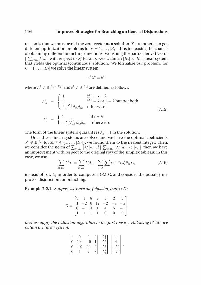
116 Improved Strategies for Branching on General Disjunctions
reason is that we must avoid the zero vector as a solution. Yet another is to getdifferent optimization problems for k = 1, . . . , |BI |, thus increasing the chanceof obtaining different branching directions. Vanishing the partial derivatives of‖
∑
i∈Rkλk
i di‖ with respect to λki for all i, we obtain an |Rk| × |Rk| linear system
that yields the optimal (continuous) solution. We formalize our problem: fork = 1, . . . , |BI |we solve the linear system
Akλk = bk,
where Ak ∈ R|Rk|×|Rk| and bk ∈ R
|Rk| are defined as follows:
Akij =
1 if i = j = k0 if i = k or j = k but not both∑|JC |
h=1 dihdjh otherwise,
bki =
{
1 if i = k
−∑|JC |
h=1 dihdkh otherwise.
(7.15)
The form of the linear system guarantees λkk = 1 in the solution.
Once these linear systems are solved and we have the optimal coefficientsλk ∈ R
|Rk| for all k ∈ {1, . . . , |BI |}, we round them to the nearest integer. Then,we consider the norm of
∑
i∈Rk
⌊
λki
⌉
di. If ‖∑
i∈Rk
⌊
λki
⌉
di‖ < ‖dk‖, then we havean improvement with respect to the original row of the simplex tableau; in thiscase, we use
∑
i∈Rk
λki xi =
∑
i∈Rk
λki xi −
∑
j∈J
∑
i ∈ Rkλki aijxj, (7.16)
instead of row ak in order to compute a GMIC, and consider the possibly im-proved disjunction for branching.
Example 7.2.1. Suppose we have the following matrix D:
D =
3 1 8 2 3 2 31 −2 0 12 −2 −4 −50 −1 4 1 4 5 −11 1 1 1 0 0 2
and we apply the reduction algorithm to the first row d1. Following (7.15), weobtain the linear system:
1 0 0 00 194 −9 10 −9 60 20 1 2 8
λ11
λ12
λ13
λ14
14−52−20
,
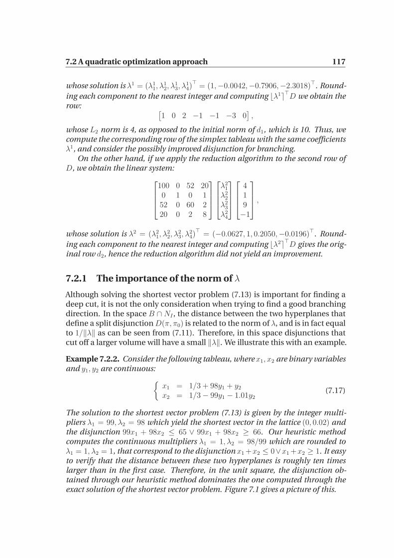
7.2 A quadratic optimization approach 117
whose solution is λ1 = (λ11, λ
12, λ
13, λ
14)⊤
= (1,−0.0042,−0.7906,−2.3018)⊤. Round-
ing each component to the nearest integer and computing ⌊λ1⌉⊤D we obtain the
row:[
1 0 2 −1 −1 −3 0]
,
whose L2 norm is 4, as opposed to the initial norm of d1, which is 10. Thus, wecompute the corresponding row of the simplex tableau with the same coefficientsλ1, and consider the possibly improved disjunction for branching.
On the other hand, if we apply the reduction algorithm to the second row ofD, we obtain the linear system:
100 0 52 200 1 0 152 0 60 220 0 2 8
λ21
λ22
λ23
λ24
419−1
,
whose solution is λ2 = (λ21, λ
22, λ
23, λ
24)⊤
= (−0.0627, 1, 0.2050,−0.0196)⊤. Round-
ing each component to the nearest integer and computing ⌊λ2⌉⊤D gives the orig-
inal row d2, hence the reduction algorithm did not yield an improvement.
7.2.1 The importance of the norm of λ
Although solving the shortest vector problem (7.13) is important for finding adeep cut, it is not the only consideration when trying to find a good branchingdirection. In the space B ∩ NI , the distance between the two hyperplanes thatdefine a split disjunction D(π, π0) is related to the norm of λ, and is in fact equalto 1/‖λ‖ as can be seen from (7.11). Therefore, in this space disjunctions thatcut off a larger volume will have a small ‖λ‖. We illustrate this with an example.
Example 7.2.2. Consider the following tableau, where x1, x2 are binary variablesand y1, y2 are continuous:
{
x1 = 1/3 + 98y1 + y2
x2 = 1/3− 99y1 − 1.01y2(7.17)
The solution to the shortest vector problem (7.13) is given by the integer multi-pliers λ1 = 99, λ2 = 98 which yield the shortest vector in the lattice (0, 0.02) andthe disjunction 99x1 + 98x2 ≤ 65 ∨ 99x1 + 98x2 ≥ 66. Our heuristic methodcomputes the continuous multipliers λ1 = 1, λ2 = 98/99 which are rounded toλ1 = 1, λ2 = 1, that correspond to the disjunction x1 +x2 ≤ 0∨x1 +x2 ≥ 1. It easyto verify that the distance between these two hyperplanes is roughly ten timeslarger than in the first case. Therefore, in the unit square, the disjunction ob-tained through our heuristic method dominates the one computed through theexact solution of the shortest vector problem. Figure 7.1 gives a picture of this.

118 Improved Strategies for Branching on General Disjunctions
x1 + x2 ≤ 0
∨ x1 + x2 ≥ 1
99x1 +98x2 ≤ 65∨ 99x1 +98x2 ≥ 66
Figure 7.1: Representation of the disjunctions discussed in Exam-ple 7.2.2.
7.2.2 Choosing the set Rk
The choice of each set Rk ⊂ BI for all k has an effect on the performance of thenorm reduction algorithm. Although using Rk = BI is possible, in that case twoproblems arise: first, the size of the linear systems may become unmanageablein practice, and second, if we add up too many rows then the coefficients onthe variables with indices in J ∩ NI may deteriorate. In particular, we may getmore nonzero coefficients. Thus, we do the following. We fix a maximum cardi-nality M|Rk|; if M|Rk| ≥ |BI |, we set Rk = BI . Otherwise, for each row k that wewant to reduce, we sort the remaining rows by ascending number of nonzerocoefficients on the variables with indices in {i ∈ J ∩NI |aki = 0}, and select thefirst M|Rk| indices as those in Rk. The reason for this choice is that, although thevalue of the coefficients on the variables with indices in J ∩NI is bounded, wewould like those that are zero in row ak to be left unmodified when we compute∑
j∈Rk
⌊
λkj
⌉
aj. As zero coefficients on those variables yield a stronger cut, weargue that this will yield a stronger split disjunction as well. During the sortingoperation, to keep computational times to a minimum we use the row numberas a tie breaker.

7.2 A quadratic optimization approach 119
7.2.3 The depth of the cut is not always a good measure
As stated earlier, the improvement in the objective function given by a GMIC is alower bound on the improvement obtained by branching on the correspondingdisjunction. We give an example showing that this lower bound may not betight and in fact the difference between these two values can be arbitrarily large.
Example 7.2.3. Consider the integer program:
min −x1 − x2
x1 ≤ 1.5x2 ≤ 1
x1/m− x2 ≥ 1.5/m− 1.25mx1 − x2 ≤ 1.5m− 0.75
x1, x2 ∈ Z,
P (7.18)
where m > 1 is a given parameter close to 1. The solution to the LP relaxation is(1.5, 1), with an objective value of −2.5. The intersection cut obtained from thedisjunction x1−x2 ≤ 0∨x1−x2 ≥ 1 is x1+x2 ≤ 2, which gives an objective value of−2. Now suppose we branch on x1−x2 ≤ 0∨x1−x2 ≥ 1. We obtain two childrenP1 and P2, which are both feasible. One can verify that optimal solution of P1 is(1.5−1.25m
1−m, 1.5−1.25m
1−m) with objective value −21.5−1.25m
1−m, and the optimal solution of
P2 is (1.5m−1.75m−1
, 0.5m−0.75m−1
) with objective value −2m−2.5m−1
. Therefore, the gap closedby branching is:
max{−21.5− 1.25m
1−m,−
2m− 2.5
m− 1} − 2.5,
which can be made arbitrarily large when m tends to 1 from above. At the sametime, the intersection cut associated with the same disjunction closes a gap of 0.5regardless of m. We give a picture of the situation for m = 1.1 in Figure 7.2.
Example 7.2.3 suggests that we should not choose the branching directionby relying on the distance cut off by the intersection cut only, even though thequality of the underlying intersection cut gives an indication of the strength ofa disjunction and can guide us towards generating better disjunctions. There-fore, in our computational experiments (see Section 7.4) we employed strongbranching to select a disjunction among those computed with the proceduredescribed so far.

120 Improved Strategies for Branching on General Disjunctions
cost function
x1/m− x2 ≥ 1.5/m−1.25
mx1− x2 ≤ 1.5m−0.75
x1 + x2 ≤ 2
x1 ≤ 1.5
x2 ≤ 1
Figure 7.2: Representation of Example 7.2.3 for m = 1.1.
7.3 A MILP formulation to generate split
disjunctions
For j ∈ J let the intersection points between the ray rj and a split disjunctionD(π, π0) be:
xj = x + αj(π, π0)rj (7.19)
LetP1,P2 be the problems at the children nodes defined by the split disjunction,and x1 and x2 be the corresponding linear relaxation optima (if Pk is infeasiblethen xk =∞ for k ∈ {1, 2}).
Lemma 7.3.1. minj∈J
c⊤xj ≤ min(c⊤x1, c⊤x2).
Proof. Let F1 = P ∩ {x ∈ Rn : π⊤x ≤ π0} and F2 = P ∩ {x ∈ R
n : π⊤x ≥ π0 + 1}be the feasible regions of, respectively, P1 and P2; we have x1 = arg min{c⊤x :c ∈ F1}, x2 = arg min{c⊤x : c ∈ F2}. Let F r
1 = P (B) ∩ {x ∈ Rn : π⊤x ≤ π0}

7.3 A MILP formulation to generate split disjunctions 121
and F r2 = P (B) ∩ {x ∈ R
n : π⊤x ≥ π0 + 1}. By the definition of the pointsxj ∀j ∈ J , we have that minj∈J{c
⊤x} = min{c⊤x : x ∈ F r1 ∪ F r
2 }. Since P ⊆ P (B),min{c⊤x : x ∈ F r
1 ∪ F r2 } ≤ min{c⊤x : x ∈ F1 ∪ F2} = min(c⊤x1, c⊤x2), which
completes the proof.
Therefore, in order to generate children nodes that have tight LP relaxations,it makes sense to try to maximize the lower bound given in Lemma 7.3.1. Inother words, we want to maximize the gap closed optimizing over the set ofsplit disjunctions. This problem can be formalized as follows.
max(π, π0) ∈ Z
n+1
π0 =¨
π⊤x˝
πi = 0∀i ∈ N \NI
minj∈J
c⊤(x + αj(π, π0)rj). (7.20)
This is a nonconvex Mixed Integer Nonlinear Problem (MINLP) where the com-plicating constraints are π0 =
⌊
π⊤x⌋
as well as the definition of αj (for all j ∈ J).We use the same simplification given in (8) and assume that αj’s numerator (seeEq. (7.5)) is fixed; for simplicity, we assume its value to be 1. Since it is the onlyterm where π0 appears, we can discard π0 from the problem altogether. Further-more, the constant c⊤x can also be discarded:
maxπ∈Zn
πi=0∀i∈N\NI
minj∈J
αj(π, π0)c⊤rj. (7.21)
Since π⊤rj = 0 means that there is no intersection between the split disjunctionand the ray rj , we can safely assume that π⊤rj 6= 0. For all j ∈ J , we introducevariables αj and constraints
αj =1
|π⊤rj|. (7.22)
The “max min” objective function is easily reformulated to:
maxπ y∀j ∈ J y ≤ αjc
⊤rj
∀j ∈ J αj = 1|π⊤rj |
∀i ∈ N \NI πi = 0π ∈ Z
n.
(7.23)
By (7.22), αj > 0 for all j ∈ J , so (7.23) can be rewritten as:
maxπ y∀j ∈ J y
αj≤ c⊤rj
∀j ∈ J |π⊤rj| = 1αj
∀i ∈ N \NI πi = 0π ∈ Z
n.

122 Improved Strategies for Branching on General Disjunctions
Remark 7.3.2. Shifting |π⊤rj| from the denominator to a numerator implicitlyremoves the constraint π⊤rj 6= 0.
Next, we introduce variables wj to replace the expression 1αj
for all j ∈ J ,
obtaining:
maxπ y∀j ∈ J wjy ≤ c⊤rj
∀j ∈ J |π⊤rj| = wj
∀i ∈ N \NI πi = 0π ∈ Z
n.
We reformulate the absolute value as follows:
maxπ y∀j ∈ J wjy ≤ c⊤rj
∀j ∈ J wj ≥ −π⊤rj
∀j ∈ J wj ≥ π⊤rj
∀i ∈ N \NI πi = 0π ∈ Z
n.
(7.24)
This is a bilinear problem of a special kind, namely one of the sets of variablesinvolved in the products only contains the single decision variable y. It is easyto see that wj > 0 for all j (it follows from the assumption π⊤rj 6= 0).
Lemma 7.3.3. For any y feasible in (7.24) we have y ≥ 0.
Proof. By the optimality conditions on x, c⊤rj ≥ 0 (i.e. the optimization direc-tion−c makes an non-acute angle with each of the rays rj), hence any y feasiblein (7.24) is such that y ≥ 0.
The case y = 0 being uninteresting (there is no guarantee of any closed gap),we restrict our attention to y > 0. This allows us to divide the constraints wjy ≤c⊤rj through by y, obtaining:
∀j ∈ J wj ≤1
yc⊤rj. (7.25)
We now introduce a positive variable z = 1y
to linearize (7.25):
∀j ∈ J wj ≤ zc⊤rj. (7.26)
This transforms the objective function in max 1z
; since this is a monotonicallydecreasing univariate function, it can be reformulated as min z. The problem

7.3 A MILP formulation to generate split disjunctions 123
now becomes a MILP:
min z∀j ∈ J wj ≤ zc⊤rj
∀j ∈ J wj ≥ −π⊤rj
∀j ∈ J wj ≥ π⊤rj
∀i ∈ N \NI πi = 0π ∈ Z
n
z ≥ 0.
(7.27)
By Remark 7.3.2, π = w = 0 and z = 0 is a feasible solution of (7.27) that ishowever infeasible in the original problem (7.20). We also have to make surethat the solution of (7.27) is a violated disjunction, i.e. π⊤x is fractional. To thisend, we add another integer variable π0, and impose the constraints that π⊤x−π0 ≥ η and π0 + 1 − π⊤x ≥ η, where η is a small positive tolerance. As for eachvector (π, π0) the symmetric one (−π,−π0 − 1) represents the same disjunction,we eliminate some symmetric solutions of the problem by imposing π0 ≥ 0. Weobtain:
min z∀j ∈ J wj ≤ zc⊤rj
∀j ∈ J wj ≥ −π⊤rj
∀j ∈ J wj ≥ π⊤rj
∀i ∈ N \NI πi = 0π⊤x− π0 ≥ η
π0 + 1− π⊤x ≥ η(π, π0) ∈ Z
n+1
π0 ≥ 0z ≥ 0.
(7.28)
In order to reduce the size of the search space and speed up the solution pro-cess, we add a constraint on the 1-norm of π, such as
∑
i∈N |πi| ≤ K. This con-straint can be reformulated in linear form by introducing two positive variables

124 Improved Strategies for Branching on General Disjunctions
π+i and π−i such that πi = π+
i − π−i ∀i ∈ N . Finally (7.28) becomes:
min z∀j ∈ J wj ≤ zc⊤rj
∀j ∈ J wj ≥ −π⊤rj
∀j ∈ J wj ≥ π⊤rj
∀i ∈ N \NI πi = 0∀i ∈ N π+
i − π−i = πi∑
i∈N(π+i + π−i ) ≤ K
π⊤x− π0 ≥ ηπ0 + 1− π⊤x ≥ η
(π, π0) ∈ Zn+1
(π+, π−) ∈ Z2n+
π0 ≥ 0z ≥ 0.
(7.29)
7.3.1 Generating a pool of split disjunctions
The MILP (7.29) is a linear approximation of the original problem (7.20), thussolving it to optimality does not guarantee to give the disjunction which maxi-mizes the lower bound in Lemma 7.3.1. Besides, in Section 7.2.3 we providedan example to show that we should not rely on the distance cut off only to evalu-ate the strength of a disjunction. Therefore, we are interested in finding severalfeasible solutions to (7.29), so as to have a large pool of split disjunctions whichcan be evaluated via strong branching to obtain the closed gap:
min(c⊤x1, c⊤x2)− c⊤x.
Some feasible solutions are typically found during the exploration of the branch-and-bound tree while solving (7.29). We repeatedly employ a local branchingapproach (56) from different starting points in order to increase the numberof feasible solutions to (7.29) computed in a short time. We now endeavour toexplain in more detail this approach.
Local branching was proposed by Fischetti and Lodi (56) as an effectiveheuristic for MILPs. The original idea only takes into account 0-1 variables,but the authors give an extension to case of general integer variables. Localbranching consists in exploring the neighbourhood of a starting feasible solu-tion by adding a local branching constraing, which limits the number of binaryvariables allowed to change their value with respect to the starting solution toat most a given parameter K. K is then the size of the neighbourhood. If thevalue of K is small, the neighbourhood is rapidly explored by MILP solvers, of-ten leading to a better solution then the original one, as shown by the compu-tational experiments in (56).
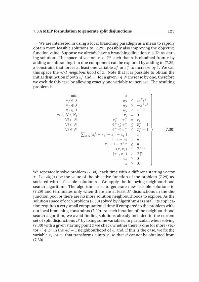
7.3 A MILP formulation to generate split disjunctions 125
We are interested in using a local branching paradigm as a mean to rapidlyobtain more feasible solutions to (7.29), possibly also improving the objectivefunction value. Suppose we already have a branching direction π ∈ Z
n as start-ing solution. The space of vectors π ∈ Z
n such that π is obtained from π byadding or subtracting 1 to one component can be explored by adding to (7.29)a constraint that forces at least one variable π+
i or π−i to increase by 1. We callthis space the +/-1 neighbourhood of π. Note that it is possible to obtain theinitial disjunction if both π+
i and π−i for a given i ∈ N increase by one, thereforewe exclude this case by allowing exactly one variable to increase. The resultingproblem is:
min z∀j ∈ J wj ≤ zc⊤rj
∀j ∈ J wj ≥ −π⊤rj
∀j ∈ J wj ≥ π⊤rj
∀i ∈ N \NI πi = 0∀i ∈ N π+
i − π−i = πi
∀i ∈ N π+i ≤ π+
i ≤ π+i + 1
∀i ∈ N π−i ≤ π−i ≤ π−i + 1∑
i∈N(π+i − π+
i + π−i − π−i ) = 1π⊤x− π0 ≥ η
π0 + 1− π⊤x ≥ η(π, π0) ∈ Z
n+1
(π+, π−) ∈ Z2n+
π0 ≥ 0z ≥ 0.
(7.30)
We repeatedly solve problem (7.30), each time with a different starting vectorπ. Let obj(π) be the value of the objective function of the problem (7.29) as-sociated with a feasible solution π. We apply the following neighbourhoodsearch algorithm. The algorithm tries to generate new feasible solutions to(7.29) and terminates only when there are at least M disjunctions in the dis-junction pool or there are no more solution neighbourhoods to explore. As thesolution space of each problem (7.30) solved by Algorithm 4 is small, its applica-tion requires a very small computational time if compared to the problem with-out local branching constraints (7.29). At each iteration of the neighbourhoodsearch algorithm, we avoid finding solutions already included in the currentset of split disjunctions D′ by fixing some variables. In particular, when solving(7.30) with a given starting point π we check whether there is one (or more) vec-tor π′ ∈ D′ in the +/ − 1 neighbourhood of π, and, if this is the case, we fix thevariable π+
i or π−i that transforms π into π′, so that π′ cannot be obtained from(7.30).
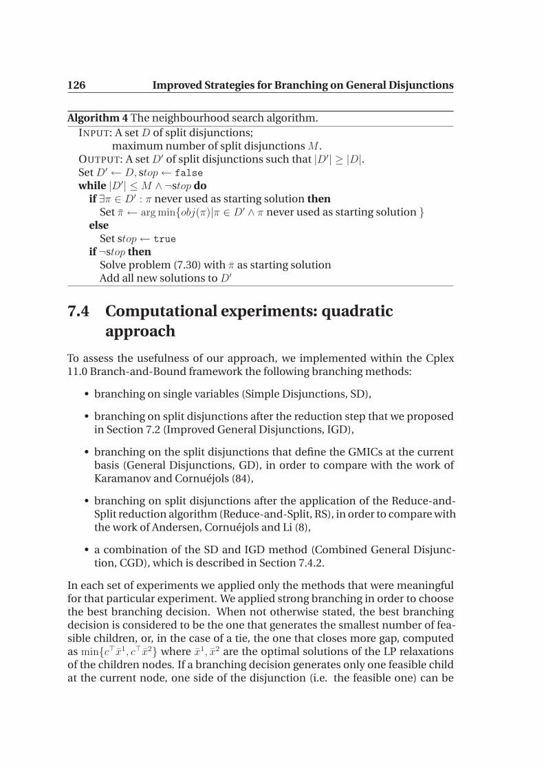
126 Improved Strategies for Branching on General Disjunctions
Algorithm 4 The neighbourhood search algorithm.
INPUT: A set D of split disjunctions;maximum number of split disjunctions M .
OUTPUT: A set D′ of split disjunctions such that |D′| ≥ |D|.Set D′ ← D, stop← false
while |D′| ≤M ∧ ¬stop doif ∃π ∈ D′ : π never used as starting solution then
Set π ← arg min{obj(π)|π ∈ D′ ∧ π never used as starting solution }else
Set stop← true
if ¬stop thenSolve problem (7.30) with π as starting solutionAdd all new solutions to D′
7.4 Computational experiments: quadratic
approach
To assess the usefulness of our approach, we implemented within the Cplex11.0 Branch-and-Bound framework the following branching methods:
• branching on single variables (Simple Disjunctions, SD),
• branching on split disjunctions after the reduction step that we proposedin Section 7.2 (Improved General Disjunctions, IGD),
• branching on the split disjunctions that define the GMICs at the currentbasis (General Disjunctions, GD), in order to compare with the work ofKaramanov and Cornuejols (84),
• branching on split disjunctions after the application of the Reduce-and-Split reduction algorithm (Reduce-and-Split, RS), in order to compare withthe work of Andersen, Cornuejols and Li (8),
• a combination of the SD and IGD method (Combined General Disjunc-tion, CGD), which is described in Section 7.4.2.
In each set of experiments we applied only the methods that were meaningfulfor that particular experiment. We applied strong branching in order to choosethe best branching decision. When not otherwise stated, the best branchingdecision is considered to be the one that generates the smallest number of fea-sible children, or, in the case of a tie, the one that closes more gap, computedas min{c⊤x1, c⊤x2} where x1, x2 are the optimal solutions of the LP relaxationsof the children nodes. If a branching decision generates only one feasible childat the current node, one side of the disjunction (i.e. the feasible one) can be
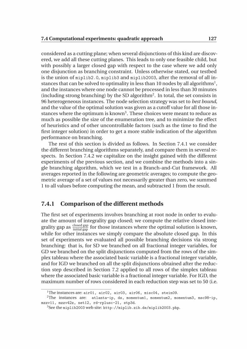
7.4 Computational experiments: quadratic approach 127
considered as a cutting plane; when several disjunctions of this kind are discov-ered, we add all these cutting planes. This leads to only one feasible child, butwith possibly a larger closed gap with respect to the case where we add onlyone disjunction as branching constraint. Unless otherwise stated, our testbedis the union of miplib2.0, miplib3 and miplib2003, after the removal of all in-stances that can be solved to optimality in less than 10 nodes by all algorithms1,and the instances where one node cannot be processed in less than 30 minutes(including strong branching) by the SD algorithm2. In total, the set consists in96 heterogeneous instances. The node selection strategy was set to best bound,and the value of the optimal solution was given as a cutoff value for all those in-stances where the optimum is known3. These choices were meant to reduce asmuch as possible the size of the enumeration tree, and to minimize the effectof heuristics and of other uncontrollable factors (such as the time to find thefirst integer solution) in order to get a more stable indication of the algorithmperformance on branching.
The rest of this section is divided as follows. In Section 7.4.1 we considerthe different branching algorithms separately, and compare them in several re-spects. In Section 7.4.2 we capitalize on the insight gained with the differentexperiments of the previous section, and we combine the methods into a sin-gle branching algorithm, which we test in a Branch-and-Cut framework. Allaverages reported in the following are geometric averages; to compute the geo-metric average of a set of values not necessarily greater than zero, we summed1 to all values before computing the mean, and subtracted 1 from the result.
7.4.1 Comparison of the different methods
The first set of experiments involves branching at root node in order to evalu-ate the amount of integrality gap closed; we compute the relative closed inte-
grality gap as closed gapinitial gap
for those instances where the optimal solution is known,
while for other instances we simply compare the absolute closed gap. In thisset of experiments we evaluated all possible branching decisions via strongbranching: that is, for SD we branched on all fractional integer variables, forGD we branched on the split disjunctions computed from the rows of the sim-plex tableau where the associated basic variable is a fractional integer variable,and for IGD we branched on all the split disjunctions obtained after the reduc-tion step described in Section 7.2 applied to all rows of the simplex tableauwhere the associated basic variable is a fractional integer variable. For IGD, themaximum number of rows considered in each reduction step was set to 50 (i.e.
1The instances are: air01, air02, air03, air06, misc04, stein09.2The instances are: atlanta-ip, ds, momentum1, momentum2, momentum3, msc98-ip,
mzzv11, mzzv42z, net12, rd-rplusc-21, stp3d.3See the miplib2003 web site: http://miplib.zib.de/miplib2003.php.

128 Improved Strategies for Branching on General Disjunctions
M|Rk| = 50∀k). The experiments were made in a bare Branch-and-Bound set-ting; that is, presolving, cutting planes and heuristics were disabled. In theseexperiments, we chose the branching decision that closed the largest gap, re-gardless of the number of feasible children. In Table 7.1 we give a summary ofthe results for this experiment. We report the average relative integrality gap
Average closed gap(on instances with known optimum)
Simple disjunctions (SD): 4.27%General disjunctions (GD): 6.71%Improved general disjunctions (IGD): 6.56%
Number of instances with largest closed gap
Simple disjunctions (SD): 58General disjunctions (GD): 64Improved general disjunctions (IGD): 70
Number of instances with one child
Simple disjunctions (SD): 10General disjunctions (GD): 29Improved general disjunctions (IGD): 27
Table 7.1: Results after branching at root node
closed by each method, the number of instances where each method closesat least the same absolute gap as the other two methods, and the number ofinstances where the disjunction that closes the largest gap generates only onefeasible child. For the first criterion we only considered instances where theoptimal solution is known, so that we could compute the relative amount of in-tegrality gap close; for the remaining criteria, we also considered the instanceswith unknown optimum. We immediately observe that branching on generaldisjunctions instead of single variables yields a significantly larger amount ofclosed integrality gap. In our experiments, the GD method closes more gap onaverage than the other two methods, and both GD and IGD clearly outperformSD under this criterion. Not only GD and IGD close more gap, but they alsomore frequently generate only one feasible child node; the number of childrenwas not taken into account when choosing the branching decision in this set ofexperiments, but it is interesting to note that with GD and IGD we often havedisjunctions that close a large amount of gap and also do not increase the sizeof the enumeration tree. Although the GD method closes slightly more gap onaverage than IGD on the instances with known optimum, if we compare thenumber of instances where each method closes at least the same amount of

7.4 Computational experiments: quadratic approach 129
gap as the other two methods then IGD ranks first with 70 instances over 96 intotal.
For many reasons, applying strong branching on all possible branching de-cisions is impractical, as it requires a very large computational effort which isnot counterbalanced by the reduction of the size of the enumeration tree. Inthe remaining experiments we evaluated the performance of the branching al-gorithms in a framework where strong branching is applied only to the mostpromising branching decisions. The number of branching decisions evaluatedwith strong branching was set to 10. In the case of SD, we picked the 10 integervariables with the largest fractionary part (i.e. closer to 0.5). For GD and IGD,we picked the 10 split disjunctions associated with the 10 GMICs that have thelargest cut off distance (equation (7.6), see (84)), where for IGD the distance wascomputed after the reduction step.
In the next two experiments, we solved up to 1000 nodes in the enumera-tion tree. We reverted back to the original branching decision selection methodthat favours those disjunctions which generate a smaller number of feasiblechildren. Having a smaller number of children is a considerable advantage aswe are able to progress further in depth of the enumeration tree, thus possi-bly leading to a larger closed gap. The evaluation criterion was the percentageof the integrality gap closed after 1000 nodes, or, if the instance was solved inless than 1000 nodes, the number of nodes required to solve to optimality. Forthis set of experiments, 7 instances4 were excluded from the testbed, as solv-ing 1000 nodes required more than 12 hours. To choose the number of rowsM|Rk| that defines the size of the linear system at each iteration of the reductionstep for the IGD method, we compared three different values: 10, 20 and 50;we included in the comparison the Reduce-and-Split (RS) coefficient improve-ment method introduced by Andersen, Cornuejols and Li (8), in order to testwhether their algorithm to generate good cutting planes was also suitable forbranching. For fairness, we used for RS the same procedure as for the IGD meth-ods: we picked the 10 split disjunctions associated with the 10 GMICs that havethe largest cut off distance after the reduction step, and applied strong branch-ing. We followed the implementation of the RS reduction algorithm given inthe CGL library (34). A summary of the results is given in Table 7.2. It can beseen that IGD using 20 or 50 rows for the reduction step yields very similar re-sults in terms of average closed gap on instances not solved by any method,and both choices close more gap than IGD with M|Rk| = 10 or RS on the un-solved instances. The average number of nodes is smaller for M|Rk| = 50. Inparticular IGD outperforms RS for branching. To investigate the reason for this,we recorded the average norm of the disjunction chosen for branching at eachnode of the enumeration tree; recall (Section 7.2.1) that the norm depends onthe coefficients λ generated by the disjunction improvement algorithm. The
4The instances are: dano3mip, fast0507, manna81, mitre, protfold, sp97ar, t1717.
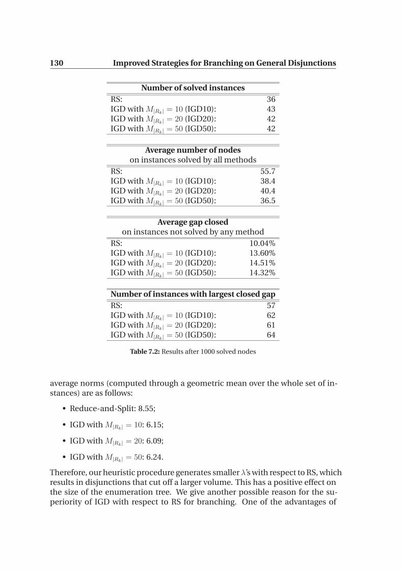
130 Improved Strategies for Branching on General Disjunctions
Number of solved instances
RS: 36IGD with M|Rk| = 10 (IGD10): 43IGD with M|Rk| = 20 (IGD20): 42IGD with M|Rk| = 50 (IGD50): 42
Average number of nodeson instances solved by all methods
RS: 55.7IGD with M|Rk| = 10 (IGD10): 38.4IGD with M|Rk| = 20 (IGD20): 40.4IGD with M|Rk| = 50 (IGD50): 36.5
Average gap closedon instances not solved by any method
RS: 10.04%IGD with M|Rk| = 10 (IGD10): 13.60%IGD with M|Rk| = 20 (IGD20): 14.51%IGD with M|Rk| = 50 (IGD50): 14.32%
Number of instances with largest closed gap
RS: 57IGD with M|Rk| = 10 (IGD10): 62IGD with M|Rk| = 20 (IGD20): 61IGD with M|Rk| = 50 (IGD50): 64
Table 7.2: Results after 1000 solved nodes
average norms (computed through a geometric mean over the whole set of in-stances) are as follows:
• Reduce-and-Split: 8.55;
• IGD with M|Rk| = 10: 6.15;
• IGD with M|Rk| = 20: 6.09;
• IGD with M|Rk| = 50: 6.24.
Therefore, our heuristic procedure generates smaller λ’s with respect to RS, whichresults in disjunctions that cut off a larger volume. This has a positive effect onthe size of the enumeration tree. We give another possible reason for the su-periority of IGD with respect to RS for branching. One of the advantages of

7.4 Computational experiments: quadratic approach 131
RS for cut generation is that the reduction algorithm generates several split dis-junctions, trying to increase the distance cut off by each one of the associatedcutting planes. As several cuts are generated at each round, this approach iseffective (8). However, at each node of a Branch-and-Bound tree only one dis-junction is chosen for branching, so a method which tries to compute only onestrong disjunction is more fruitful than one that generates a set of several pos-sibly weaker ones. This, combined with smaller coefficient λ’s at the end of thereduction procedure, may explain why the algorithm described in Section 7.2seems to be more effective than RS for branching. We decided to use IGD withM|Rk| = 50 in all following experiments. We did not test larger values of the pa-rameter, since solving the linear system would take too much time in practice.
A summary of the comparison between SD, GD and IGD with M|Rk| = 50can be found in Table 7.3. The increase in the gap per node that can be closed
Number of solved instances
Simple disjunctions (SD): 35General disjunctions (GD): 42Improved general disjunctions (IGD): 42
Average number of nodeson instances solved by all methods
Simple disjunctions (SD): 92.7General disjunctions (GD): 52.9Improved general disjunctions (IGD): 43.2
Average gap closedon instances not solved by any method
Simple disjunctions (SD): 9.36%General disjunctions (GD): 13.78%Improved general disjunctions (IGD): 14.15%
Number of instances with largest closed gap
Simple disjunctions (SD): 55General disjunctions (GD): 56Improved general disjunctions (IGD): 63
Table 7.3: Results after 1000 solved nodes
by branching on general disjunctions with respect to branching on single vari-ables is large. This is confirmed by the results in (84). Besides, the IGD methodseems to be on average superior in all respects to the other two methods, as it

132 Improved Strategies for Branching on General Disjunctions
closes more gap for the unsolved instances under 1000 nodes, and requires lessnodes for the solved instances. This is also evident if we compare the number ofinstances where each method closes at least the same absolute gap as the othertwo methods: IGD ranks first with 63 instances over the 89 instances in the test-set. However, there are two instances where branching on simple disjunctionsis more profitable than branching on general disjunctions: the air04 and air05
instances are solved by the SD method in 225 and 139 nodes respectively, whileGD and IGD do not manage to solve them in 1000 nodes. All other instanceswhich are solved by SD are also solved by GD and IGD.
7.4.2 Combination of several methods
Results in Table 7.3 suggest that IGD is indeed capable of closing more gap pernode on a large number of instances; however, a more detailed analysis of theresults shows that there are a few instances where branching on general dis-junctions is not profitable, and thus both GD and IGD perform poorly. Thismay also happen, for example, in zero gap instances, where the enumerationof nodes with SD is usually more effective. Thus, we decided to combine boththe SD and the IGD method into a single branching algorithm which tries to de-cide, for each instance, if it is more effective to branch on simple disjunctionsor on general disjunctions. First we describe the ideas and the practical consid-erations behind the algorithm, and then we will describe how we implementedit.
The most evident drawback of branching on general disjunctions is that it isslower than using simple disjunctions. It is slower in several respects: the firstreason is that the computations at each node take longer. This is because wehave to compute the distance cut off by the GMIC associated with each row ofthe simplex tableau, and the reduction step that we propose involves the solu-tion of an M|Rk|×M|Rk| linear system for each row which is improved, where wechose M|Rk| = 50. All these computations are carried out several times, thus theoverhead per node with respect to branching on simple disjunctions is signifi-cant. The second reason is that, by branching on general disjunction, we addone (or more) rows to the formulation of children nodes, which may result ina slowdown of the LP solution process. On the other hand, branching on sim-ple disjunctions involves only a change in the bounds of some variables, thusthe size of the LP does not increase. This suggests that branching on generaldisjunctions should be used only if it is truly profitable, which in turn requiresa measure of profit. We decided to use the amount of closed gap as a measureof profit. Besides, since the computational overhead per node is significantwhen considering general disjunctions for branching, we would like to considerthem only if it brings an improvement in the solution time. Thus, if on a giveninstance general disjunctions are never used because simple disjunctions aremore profitable, we would like to disable their computation as soon as possible

7.4 Computational experiments: quadratic approach 133
Algorithm 5 CGD branching algorithm
Initialization: ActiveGDCounter ← 3, FailedActivation ← 0, NodeCounter ←0while branching do
if root node thenNumGD ← 20, NumSD ← 20
elseif ActiveGDCounter > 0 then
NumGD ← 7, NumSD ← 3else
NumGD ← 0, NumSD ← 10generate NumGD general disjunctionsgenerate NumSD simple disjunctionsfor all branching decisions do
apply strong branchingchoose a disjunction D(π, π0)if ActiveGDCounter > 0 then
if D(π, π0) has support > 1 thenActiveGDCounter ← 10FailedActivation← 0
elseActiveGDCounter ← ActiveGDCounter − 1if ActiveGDCounter = 0 then
FailedActivation← FailedActivation + 1else
NodeCounter ← NodeCounter + 1if FailedActivation < 10 ∧NodeCounter = 100 then
ActiveGDCounter ← 1NodeCounter ← 0
in the enumeration tree. As the polyhedron underlying a problem may signifi-cantly change in different parts of the branching tree, it may be a good idea totest branching on general disjunctions periodically even if it has been disabled,in order to verify whether it has become profitable.
We implemented a branching algorithm based on the above considerationsin the following way: at each node, branching on general disjunctions can beactive or not. If it is active, we test 10 possible branching decisions with strongbranching: 7 general disjunctions, and 3 simple disjunctions. General disjunc-tions are picked only if they generate a smaller amount of children nodes, or(in case of a tie) if the amount of closed gap is at least 50% larger. As a conse-quence, at all nodes where we do not manage to close any gap we always prefersimple disjunctions if they generate the same number of children as general
134 Improved Strategies for Branching on General Disjunctions
disjunctions. At the beginning of the enumeration tree, branching on generaldisjunctions is active for the first 3 nodes; moreover, we put an increased ef-fort at root node, where we consider up to 20 simple disjunctions and 20 gen-eral disjunctions. Whenever a general disjunction is chosen for branching, thenbranching on general disjunctions is activated for the following 10 nodes. Oth-erwise, when it is disactivated (because of simple disjunctions being preferredto general disjunctions for a given number of consecutive nodes, i.e. 3 at thebeginning of the enumeration tree, 10 otherwise), it is reactivated again after100 nodes, but only for one node, in order to test whether in that part of theenumeration tree general disjunctions are worthwhile. If a general disjunctionis chosen, then branching on general disjunctions is reactivated for the follow-ing 10 nodes. After 10 consecutive unfruitful activations, i.e. general disjunc-tions are not chosen after being activated for 10 consecutive times, branchingon general disjunctions is permanently disabled. When performing the reduc-tion step described in Section 7.2, in order to save time we do not consider allrows for reduction, but only the most promising ones. We do this by lookingat the GMIC associated with each row where the basic integer variable is frac-tional, and sorting them by the corresponding distance cut off (7.6). The 10rows (20 at root node) with the largest distance are modified with the reductionstep of Section 7.2. Since only 7 have to be selected for strong branching, werecompute the distances and pick the 7 largest ones. We give a description ofthis algorithm in Algorithm 5.
To assess the practical usefulness of this approach, we compared this branch-ing algorithm, which we will call Combined General Disjunctions (CGD), withSD. In order to evaluate the same number of branching decisions via strongbranching with both methods at each node, we modified SD in order to con-sider, at root node, the branching decisions corresponding to the 40 integervariables with largest fractional part, and then reverting back to the usual 10 forthe following nodes. We let Cplex 11.0 apply cutting planes at root node withthe default parameters, and then branched for two hours. Again, preprocessingand heuristics were disabled. In Table 7.4 we compare the number of solvedinstances within the two hours limit, the average closed gap on instances notsolved by either method, the average number of nodes and average CPU timeon instances solved by both methods. The results clearly indicate that the CGDis able to combine the potential of the IGD method to close more gap with therapidity of branching on simple disjunctions when general disjunctions are notworth the additional required time. Not only CGD solves all instances solvedby SD, but it solves 3 more: 10teams in 273.46 seconds of CPU time, gesa2 o in2616.2 seconds, and rout in 2540.74 seconds. On the instances which have notbeen solved by either of the two methods, the average integrality gap closed byCGD is 31% larger in relative terms than the one closed by SD. This result is evenmore important if we consider that CGD is slower: in the 2 hours limit CGDsolved only half as many nodes as SD on average, thus the gap closed per node

7.4 Computational experiments: quadratic approach 135
Number of solved instances
Simple disjunctions (SD): 67Combined general disjunctions (CGD): 70
Average number of nodeson instances solved by both methods
Simple disjunctions (SD): 195.1Combined general disjunctions (CGD): 98.0
Average number of nodeson instances not solved by either method
Simple disjunctions (SD): 35796.0Combined general disjunctions (CGD): 15075.7
Average gap closedon instances not solved by either method
Simple disjunctions (SD): 5.35%Combined general disjunctions (CGD): 7.03%
Average CPU time [sec]on instances solved by both methods
Simple disjunctions (SD): 3.03Combined general disjunctions (CGD): 3.35
Table 7.4: Results in a Branch-and-Cut framework with a two hourstime limit
is significantly larger for CGD. These average values only take into account theinstances with known optimum value.
We report a full table of results on the instance that have not been solvedin less than two hours by the SD method in Table 7.5. If we consider the 5instances for which the optimal solution value is not known, then on the liu
instance both methods close the same absolute gap, on dano3mip CGD closesmore gap, and on the remaining 3 instances (sp97ar, t1717, timtab2) SD closesmore gap. However, on all 5 instances CGD solves a smaller amount of nodes
since it is slower, and the relative difference (i.e. absolute gap SDabsolute gap CGD
− 1) in closed
gap on the 3 instances where SD closes more gap is small: on timtab2, the dif-ference is only 0.13%, but CGD requires 4 times fewer nodes; on sp97ar thedifference is 4.95% in favour of SD, but CGD requires 13 times fewer nodes. Thedifference increases on the t1717 instance: SD closes in relative terms 12.99%
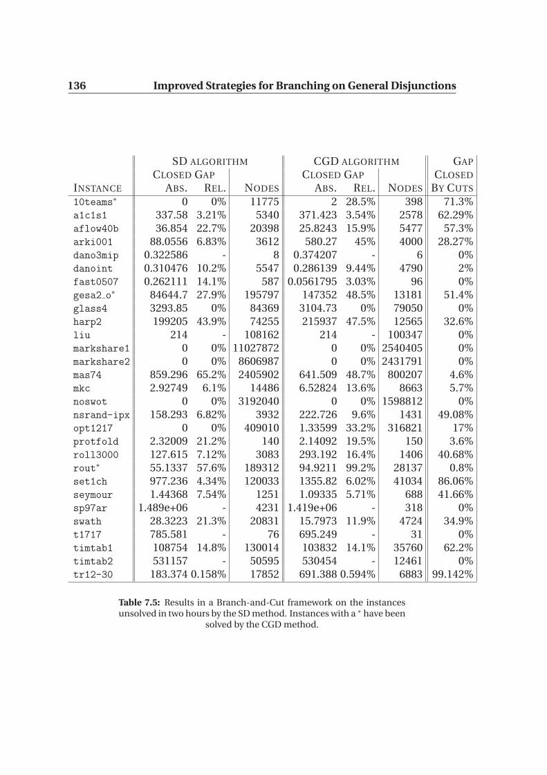
136 Improved Strategies for Branching on General Disjunctions
SD ALGORITHM CGD ALGORITHM GAP
CLOSED GAP CLOSED GAP CLOSED
INSTANCE ABS. REL. NODES ABS. REL. NODES BY CUTS
10teams∗ 0 0% 11775 2 28.5% 398 71.3%a1c1s1 337.58 3.21% 5340 371.423 3.54% 2578 62.29%aflow40b 36.854 22.7% 20398 25.8243 15.9% 5477 57.3%arki001 88.0556 6.83% 3612 580.27 45% 4000 28.27%dano3mip 0.322586 - 8 0.374207 - 6 0%danoint 0.310476 10.2% 5547 0.286139 9.44% 4790 2%fast0507 0.262111 14.1% 587 0.0561795 3.03% 96 0%gesa2 o∗ 84644.7 27.9% 195797 147352 48.5% 13181 51.4%glass4 3293.85 0% 84369 3104.73 0% 79050 0%harp2 199205 43.9% 74255 215937 47.5% 12565 32.6%liu 214 - 108162 214 - 100347 0%markshare1 0 0% 11027872 0 0% 2540405 0%markshare2 0 0% 8606987 0 0% 2431791 0%mas74 859.296 65.2% 2405902 641.509 48.7% 800207 4.6%mkc 2.92749 6.1% 14486 6.52824 13.6% 8663 5.7%noswot 0 0% 3192040 0 0% 1598812 0%nsrand-ipx 158.293 6.82% 3932 222.726 9.6% 1431 49.08%opt1217 0 0% 409010 1.33599 33.2% 316821 17%protfold 2.32009 21.2% 140 2.14092 19.5% 150 3.6%roll3000 127.615 7.12% 3083 293.192 16.4% 1406 40.68%rout∗ 55.1337 57.6% 189312 94.9211 99.2% 28137 0.8%set1ch 977.236 4.34% 120033 1355.82 6.02% 41034 86.06%seymour 1.44368 7.54% 1251 1.09335 5.71% 688 41.66%sp97ar 1.489e+06 - 4231 1.419e+06 - 318 0%swath 28.3223 21.3% 20831 15.7973 11.9% 4724 34.9%t1717 785.581 - 76 695.249 - 31 0%timtab1 108754 14.8% 130014 103832 14.1% 35760 62.2%timtab2 531157 - 50595 530454 - 12461 0%tr12-30 183.374 0.158% 17852 691.388 0.594% 6883 99.142%
Table 7.5: Results in a Branch-and-Cut framework on the instancesunsolved in two hours by the SD method. Instances with a ∗ have been
solved by the CGD method.

7.4 Computational experiments: quadratic approach 137
more gap than CGD, solving twice as many nodes in the two hours limit.On a few instances, CGD performs strikingly better than SD. Examples are
the arki001 and opt1217 instances, which are difficult instances of miplib2003.For arki001, branching with CGD closes 45% of the gap, whereas branchingwith SD only closes 6.83%. Similarly, for opt1217 CGD closes 33.2%, versus0% for SD. The arki001 instance was first solved to optimality only recentlyby Balas and Saxena (13): they invest a large computational effort in order togenerate rank-1 split cuts that close 83.05% of the integrality gap, and then useCplex’s Branch-and-Bound algorithm to close the remaining gap (16.95%) in643425 nodes. We report that, if we run CGD on arki001 without time limits,28.27% of the integrality gap is closed by Cplex’s cutting planes with default pa-rameters, while the remaining 71.73% is closed by our branching algorithm in925738 nodes. Note that Balas and Saxena used the preprocessed problem asinput, while in this chapter we always work with the original instances (i.e. with-out preprocessing). 10teams, gesa2 o, harp2, rout and tr12-30 are five other in-stances where CGD greatly outperforms SD. Among examples that were solvedby both algorithms (see Table 7.6), bell3a required 15955 nodes using SD ver-sus only 20 using CGD, bell5 required 773432 nodes using SD versus 24 usingCGD, and gesa2 required 38539 nodes using SD versus 140 using CGD. Thereis also an improvement in computing time by several orders of magnitude onthese three instances.
On those instances which are solved by both methods, CGD requires on av-erage only half the nodes needed by SD, and the average CPU time is very closefor both methods (with a slight advantage for SD). Full results are reported inTable 7.6.
Summarizing, in our experiments the combination between SD and IGD,which we have called CGD, seems clearly superior to the traditional branch-ing strategy that is represented by branching on single variables. Moreover, asCplex’s callable library is not optimized for branching on general disjunctions,the implementation of CGD could be made faster.
GAP CLOSED SD ALGORITHM CGD ALGORITHM
BY CUTS BY BRANCHING TIME TIME
INSTANCE ABS. REL. NODES [SEC] NODES [SEC]
aflow30a 65.9% 59.6358 34.1% 1813 77.886 1725 99.839air04 17.9% 494.084 82.1% 181 164.972 203 683.874air05 15.1% 421.787 84.9% 209 105.902 241 133.679bell3a 70.8% 4638.26 29.2% 15955 11.822 20 0.047bell3b 89.6% 39855.3 10.4% 1206 2.177 526 5.512bell4 91.93% 44957.8 8.07% 9091 24.177 3636 24.242bell5 85.6% 51456.8 14.4% 773432 553.703 24 0.128blend2 23.2% 0.524858 76.8% 539 5.321 454 9.920bm23 24.8% 10.0974 75.2% 119 0.272 78 0.364cap6000 37.6% 113.47 62.4% 289 30.176 236 111.553dcmulti 68.5% 1323.83 31.5% 41 1.050 56 2.853

138 Improved Strategies for Branching on General Disjunctions
GAP CLOSED SD ALGORITHM CGD ALGORITHM
BY CUTS BY BRANCHING TIME TIME
INSTANCE ABS. REL. NODES [SEC] NODES [SEC]
dsbmip 100% 0 0% 15 1.666 23 2.754egout 35.7% 568.101 64.3% 1 0.009 1 0.011fiber 91.83% 20400.8 8.17% 153 3.944 28 4.025fixnet3 97.98% 227.43 2.02% 5 0.300 5 0.421fixnet4 87.7% 573.738 12.3% 33 1.438 52 8.526fixnet6 83.4% 461.791 16.6% 1087 20.417 1365 52.859flugpl 11.8% 30286.3 88.2% 199 0.074 16 0.021gen 100% 112313 0% 0 0.021 0 0.026gesa2 74.9% 76271.3 25.1% 38539 1232.150 140 28.490gesa3 69.3% 48425.7 30.7% 51 2.149 63 4.016gesa3 o 70.9% 45960.5 29.1% 89 3.934 34 9.955gt2 91.65% 643.634 8.35% 236 0.412 43 0.139khb05250 99.9336% 7317.49 0.0664% 5 0.106 2 0.105l152lav 30.1% 65.4949 69.9% 552 15.614 149 16.251lp4l 76% 5.875 24% 3 0.059 3 0.160lseu 68.1% 91.0289 31.9% 61 0.181 46 0.349manna81 100% 0 0% 0 0.143 0 0.147mas76 4.2% 1065.02 95.8% 309659 651.702 377398 2608.890misc01 44.5% 281.057 55.5% 251 3.836 274 7.151misc02 56.6% 295.312 43.4% 19 0.148 10 0.191misc03 9.8% 1308.17 90.2% 255 3.73 496 11.875misc05 45.2% 29.3913 54.8% 103 1.658 33 0.823misc06 26.5% 6.83269 73.5% 17 1.110 17 2.365misc07 5.8% 1313.75 94.2% 12139 462.649 25940 1536.48mitre 100% 0 0% 15 4.394 15 10.759mod008 21.9% 12.5493 78.1% 345 0.937 13 0.095mod010 28% 11.5 72% 25 0.567 2 0.440mod011 68.2% 2.40503e+06 31.8% 707 2633.340 250 3539.000mod013 30.1% 17.4348 69.9% 115 0.317 107 0.422modglob 73.7% 81583 26.3% 1879 48.692 2387 75.699nw04 9.1% 501.358 90.9% 83 75.879 48 109.610p0033 99.9159% 0.478261 0.0841% 3 0.005 3 0.007p0040 100% 62027 0% 0 0.002 0 0.001p0201 46% 400 54% 69 1.147 50 1.635p0282 96.99% 2458.44 3.01% 23 0.218 12 0.261p0291 48.5% 5223.75 51.5% 0 0.017 0 0.018p0548 99.9274% 6.08471 0.0726% 9 0.076 6 0.157p2756 98.49% 6.56956 1.51% 7 0.364 13 1.205pipex 63.5% 5.30334 36.5% 19 0.041 12 0.050pk1 0% 11 100% 243317 956.355 189740 1468.170pp08aCUTS 87.1% 240.666 12.9% 711 12.363 658 18.583pp08a 94.38% 258.537 5.62% 392 4.633 372 4.481qiu 0% 798.766 100% 19399 2780.000 19399 2901.890qnet1 71% 509.709 29% 53 3.156 74 26.939qnet1 o 85.1% 585.272 14.9% 17 1.267 13 3.826rentacar 51% 759381 49% 11 12.047 11 14.973rgn 15.9% 28.0903 84.1% 2089 2.143 1703 3.826sample2 46.5% 68.4556 53.5% 35 0.092 33 0.103sentoy 24.9% 50.6089 75.1% 52 0.175 53 0.266

7.5 Computational experiments: MILP formulation 139
GAP CLOSED SD ALGORITHM CGD ALGORITHM
BY CUTS BY BRANCHING TIME TIME
INSTANCE ABS. REL. NODES [SEC] NODES [SEC]
set1al 99.9521% 2.2619 0.0479% 5 0.056 6 0.145set1cl 34.7% 6484.25 65.3% 0 0.021 0 0.023stein15 0% 2 100% 42 0.058 44 0.068stein27 0% 5 100% 1628 3.785 1537 3.721stein45 0% 8 100% 29676 218.862 28882 215.015vpm1 89.1% 0.5 10.9% 17 0.092 17 0.107vpm2 77% 0.888645 23% 1299 15.646 477 5.723
Table 7.6: Results in a Branch-and-Cut framework on the instancessolved by both the SD and the CGD method.
7.5 Computational experiments: MILP
formulation
We implemented a branching scheme based on the formulation described inSection 7.3 with the neighbourhood search algorithm of Section 7.3.1 withinCplex 11.0 (83). In this section we provide preliminary computational experi-ments.
We modified Cplex’s branching algorithm so to execute, at each node of thenumeration tree, the following steps:
1. Set up the auxiliary problem (7.29) using the optimal basis of the LP relax-ation at the current node
2. Solve the auxiliary problem (7.29) with Cplex’s branch-and-cut algorithmfor a limited number of nodes, emphasizing the use of heuristics, to ob-tain an initial set of solutions
3. Apply Algorithm 4 to generate more solutions via local search
4. Apply strong branching to all candidates to select the best disjunctionwith respect to a given criterion
We set K = 10 and η = 0.05 in (7.29). We recall that K is an upper boundon the 1-norm of the disjunctions, and η is the minimum amount by whicheach disjunction should be violated. At step 2), we limit the solution processto 60 seconds or 1000 nodes, whichever comes first. The maximum number ofdisjunctions generated by Algorithm 4 was set to M = 20. Let x1, x2 be theoptimal solutions to the LP relaxations of the children that would be gener-ated by branching on a disjunction; we select the disjunction that maximizesmin(c⊤x1, c⊤x2) among all candidates.
140 Improved Strategies for Branching on General Disjunctions
In the formulation of the auxiliary problem (7.29), some changes can helpdecreasing the computational burden. First, since ∀i ∈ N \ NI we must haveπi = 0, we can drop the variables πi for i ∈ N \NI . Next, the variables πi, i ∈ NI
can be dropped and replaced by π+i − π−i . Finally, the variables wj∀j ∈ J can
be dropped, and the constraints ∀j ∈ J wj ≤ zc⊤rj,∀j ∈ J wj ≥ −π⊤rj,∀j ∈J wj ≥ π⊤rj can be replaced with ∀j ∈ J zc⊤rj ≥ −π⊤rj,∀j ∈ J zc⊤rj ≥ π⊤rj .
In the following, we apply different branching methods to a set of 78 hetero-geneous instances taken from miplib2.0, miplib3, miplib2003. Cutting planesand heuristics are disabled; thus, we apply a pure branch-and-bound schemefor 1000 nodes, and compare the amount of integrality gap closed after 1000nodes or, in case the instance is solved before this limit, the number of nodesin the enumeration tree. The split disjunctions are generated with three dif-ferent methods: the one described above based on the formulation of Section7.3, which we call the MILP method; the heuristic procedure with a quadraticformulation described in Section 7.4.2, which we call the IGD method; the tra-ditional branching scheme of selecting integer variables with fractional valuesin the current solution, and considering the corresponding simple disjunction,which we call the SD method.
Table 7.7 summarizes the results; details can be found in Table 7.8. All av-erages are geometric. For the SD method, strong branching was applied to allinteger variables with fractional value. As confirmed by Section 7.4, the averagevalues clearly indicate that branching on general disjunctions is very effectiveif compared to branching on simple disjunctions. The number of nodes forthe instances solved by all methods is significantly smaller for the IGD method,which in general seems to perform better than SD and MILP. In particular, IGDsolves 3 more instances with respect to MILP; these are the bell instances,where MILP does not perform as well as IGD. Moreover, IGD requires signifi-cantly fewer nodes than SD and MILP on the instances which are solved by allmethods. On the other hand, MILP ranks first in terms of gap closed on the un-solved instances, which suggests that MILP shows good results on the difficultinstances. MILP also ranks first if comparing the number of instances on whicheach method closes an absolute gap which is at least as large as the gap closedby the other two methods. Indeed, MILP closes more gap than IGD and SDon the following instances with medium to hard difficulty: a1c1s1, arki001,
fixnet3, fixnet6, gesa2, gesa2 o, mkc, pp08aCUTS, pp08a, tr12-30. How-ever, MILP requires significantly more time: on average, on the instances whichare unsolved in less than 1000 nodes by neither MILP nor IGD, MILP requires4700 seconds of CPU time, whereas IGD requires only 45. We note that, al-though the neighbourhood search phase should ideally iterate until M = 20split disjunctions are generated, the arithmetic average number of disjunctionsgenerated each node is 16.36. This indicates that the neighbourhood search al-gorithm often terminates because of lack of starting solutions.
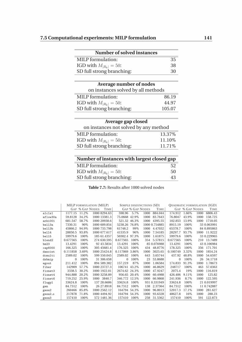
7.5 Computational experiments: MILP formulation 141
Number of solved instances
MILP formulation: 35IGD with M|Rk| = 50: 38SD full strong branching: 30
Average number of nodeson instances solved by all methods
MILP formulation: 86.19IGD with M|Rk| = 50: 44.97SD full strong branching: 105.07
Average gap closedon instances not solved by any method
MILP formulation: 13.37%IGD with M|Rk| = 50: 11.10%SD full strong branching: 11.71%
Number of instances with largest closed gap
MILP formulation: 52IGD with M|Rk| = 50: 50SD full strong branching: 43
Table 7.7: Results after 1000 solved nodes
MILP FORMULATION (MILP) SIMPLE DISJUNCTIONS (SD) QUADRATIC FORMULATION (IGD)GAP % GAP NODES TIME GAP % GAP NODES TIME GAP % GAP NODES TIME
a1c1s1 1177.15 11.2% 1000 8294.63 598.96 5.7% 1000 884.044 174.912 1.66% 1000 6806.43aflow30a 59.8128 34.2% 1000 13381.3 75.0668 42.9% 1000 83.7643 76.8047 43.9% 1000 158.725arki001 681.547 58.7% 1000 20938.6 521.32 46.3% 1000 4395.55 102.853 13.9% 1000 1718.05bell3a 7330.31 90% 1000 609.854 5238.26 76.8% 1000 0.754885 8915.19 100% 33 0.063991bell3b 45866.2 94.9% 1000 733.798 61748.2 99% 1000 4.47032 65378.7 100% 84 0.895863bell4 28850.5 93.8% 1000 677.617 41535.9 96% 1000 7.54185 28297.7 93.7% 1000 11.9222bell5 59979.6 100% 185 61.4357 50302.4 97.3% 1000 1.61875 59979.6 100% 33 0.229965blend2 0.677565 100% 274 630.595 0.677565 100% 354 5.57815 0.677565 100% 210 13.7489bm23 13.4291 100% 92 43.5834 13.4291 100% 85 0.076988 13.4291 100% 43 0.106984cap6000 166.325 100% 305 45681.4 176.325 100% 434 48.8776 178.325 100% 356 171.701danoint 0.111858 3.69% 1000 25424.8 0.117069 3.86% 1000 3025.65 0.100749 3.32% 1000 1854.24dcmulti 2589.02 100% 599 550.045 2589.02 100% 643 3.65744 437.92 48.8% 1000 54.6597dsbmip 0 100% 31 306.658 0 100% 23 53.8688 0 100% 26 34.1718egout 211.412 100% 894 589.382 157.219 87% 1000 1.06584 174.833 91.3% 1000 1.78673fiber 142909 57.7% 1000 23727.3 106741 43.2% 1000 46.8629 248717 100% 463 57.0363fixnet3 3338.5 30.2% 1000 1922.01 2674.62 24.3% 1000 47.9247 2075.4 19% 1000 116.819fixnet4 944.888 20.2% 1000 3258.89 956.65 20.4% 1000 60.4988 426.406 9.11% 1000 125.82fixnet6 719.252 25.9% 1000 3840.7 346.772 12.5% 1000 66.9868 241.936 8.7% 1000 122.595flugpl 33624.8 100% 137 28.6606 33624.8 100% 931 0.331949 33624.8 100% 21 0.019997gen 84.7312 100% 26 27.8918 84.7312 100% 138 2.37364 84.7312 100% 11 0.742887gesa2 260466 85.8% 1000 2562.12 164794 54.3% 1000 96.8013 52017.3 17.1% 1000 281.627gesa2 o 217878 71.8% 1000 4494.92 164794 54.3% 1000 93.6328 48627.8 16% 1000 288.23gesa3 157410 100% 572 1481.36 157410 100% 258 31.5362 157410 100% 591 122.873

142 Improved Strategies for Branching on General Disjunctions
MILP FORMULATION (MILP) SIMPLE DISJUNCTIONS (SD) QUADRATIC FORMULATION (IGD)GAP % GAP NODES TIME GAP % GAP NODES TIME GAP % GAP NODES TIME
gesa3 o 157410 100% 432 2031.91 157410 100% 286 29.0646 157410 100% 958 181.184glass4 7.987e-06 0% 1000 6069.47 1100 0% 1000 41.3407 7.987e-06 0% 1000 35.0307gt2 7705.77 100% 193 425.666 7705.77 100% 99 0.164974 7705.77 100% 34 0.153976harp2 180686 46% 1000 102603 203908 51.1% 1000 36.4025 123485 33.4% 1000 121.588khb05250 1.102e+07 100% 921 1022.84 1.102e+07 100% 723 10.6674 1.102e+07 100% 611 17.7793liu 214 - 1000 21114.4 214 - 1000 284.748 0 - 1000 723.5lp4l 5.18831 100% 4 94.5356 5.18831 100% 4 0.098984 5.18831 100% 2 0.086986lseu 285.318 100% 828 922.694 171.462 60.1% 1000 1.11083 285.318 100% 64 0.364945manna81 1 0.751% 1000 85790.8 1.5 1.13% 1000 6193.58 0.5 0.376% 298 14436.2markshare1 0 0% 1000 2070.21 0 0% 1000 0.670898 0 0% 1000 8.66268markshare2 0 0% 1000 3715.36 0 0% 1000 0.894863 0 0% 1000 11.9542mas74 172.912 13.1% 1000 6548.5 200.418 15.2% 1000 6.32704 221.672 16.8% 1000 13.9729mas76 193.882 17.4% 1000 5344.13 180.767 16.3% 1000 4.42533 244.732 22% 1000 10.8833misc01 506.5 100% 111 171.165 506.5 100% 137 0.85387 506.5 100% 83 1.3138misc02 680 100% 16 7.2159 680 100% 15 0.045993 680 100% 11 0.096985misc03 1450 100% 159 558.287 1450 100% 138 2.97655 1450 100% 188 7.15491misc05 53.6 100% 22 18.6892 53.6 100% 72 0.942856 53.6 100% 44 1.50777misc06 9.17135 100% 43 58.8371 9.17135 100% 20 0.492925 9.17135 100% 16 1.36079misc07 215.714 15.5% 1000 16089.5 51.6667 3.7% 1000 203.662 119.167 8.54% 1000 155.163mkc 39.38 82% 1000 87308.4 38.43 80% 1000 404.27 30 62.5% 1000 3764.3mod008 16.0689 100% 361 1877.13 9.865 61.4% 1000 1.16782 16.0689 100% 17 0.061991mod010 15.9167 100% 9 1122.47 15.9167 100% 23 1.08083 15.9167 100% 3 0.45993mod013 24.9333 100% 185 149.338 24.9333 100% 227 0.177972 24.9333 100% 54 0.141979modglob 131127 42.3% 1000 1608.1 131595 42.5% 1000 51.8241 85446.9 27.6% 1000 41.4137noswot 0 0% 1000 944.83 0 0% 1000 3.17852 0 0% 1000 12.2511opt1217 0.272819 6.78% 1000 80674.2 0 0% 1000 13.47 1.92367 47.8% 1000 51.3492p0033 568.428 100% 143 69.2525 568.428 100% 261 0.06399 568.428 100% 21 0.016997p0040 225.618 100% 6 2.76158 225.618 100% 31 0.009999 225.618 100% 2 0.002p0201 740 100% 106 602.537 740 100% 70 1.40979 740 100% 40 1.15882p0282 81543.5 100% 72 77.1203 81543.5 100% 42 0.162975 81543.5 100% 57 0.478928p0291 2994.65 100% 18 13.9899 2994.65 100% 21 0.050992 2994.65 100% 12 0.047993p0548 8136.34 100% 762 2550.91 8136.34 100% 784 4.17037 8136.34 100% 121 2.25266p2756 3.21948 3.08% 1000 31487.3 2.19718 2.85% 1000 87.2827 3.52113 3.15% 1000 292.204pipex 14.5119 100% 71 62.9474 14.5119 100% 325 0.167974 14.5119 100% 13 0.029996pk1 0 0% 1000 2695.28 0 0% 1000 7.61684 0 0% 1000 23.2875pp08aCUTS 680.439 36.4% 1000 2422 612.248 32.7% 1000 61.4507 417.95 22.4% 1000 45.8pp08a 1332.14 28.9% 1000 901.196 1236 26.9% 1000 13.7629 1128.5 24.5% 1000 23.1855rgn 33.4 100% 847 816.246 33.4 100% 859 0.898863 33.4 100% 568 1.44878rout 14.7457 15.4% 1000 27213.4 19.8707 20.8% 1000 92.168 53.4079 55.8% 1000 116.207sample2 128 100% 157 46.4479 128 100% 93 0.054991 128 100% 87 0.105984sentoy 67.278 100% 63 60.4588 67.278 100% 54 0.072989 67.278 100% 35 0.122982set1al 364.408 17.3% 1000 1513.83 423.136 18.6% 1000 147.961 312.342 16.2% 1000 260.723set1ch 2102.43 23.1% 1000 2664.5 1842.41 22% 1000 147.174 1244.09 19.3% 1000 174.753set1cl 359.619 18.1% 1000 1311.85 356.628 18% 1000 113.272 300.171 16.9% 1000 259.563stein15 2 100% 38 7.61984 2 100% 44 0.069989 2 100% 31 0.066989stein27 2 40% 1000 294.986 3 60% 1000 4.03639 5 100% 865 3.42748stein45 1 12.5% 1000 788.01 2.33333 29.2% 1000 39.0691 2.09804 26.2% 1000 23.8184timtab1 53915 7.32% 1000 3395.07 119678 16.3% 1000 29.0176 123309 16.8% 1000 58.1322timtab2 14394 - 1000 7475.45 83794 - 1000 92.131 93552 - 1000 211.767tr12-30 3666.48 6.51% 1000 3079.88 3014.82 5.95% 1000 1169.3 1289.27 4.47% 1000 958.276vpm1 4.58333 100% 21 26.9529 1.15 25.1% 1000 6.46402 4.58333 100% 25 0.259961vpm2 1.39564 39.6% 1000 2057.29 1.34673 38.3% 1000 14.6928 1.50242 42.4% 1000 27.2479
Table 7.8: Results after 1000 solved nodes: full results
Several reasons suggest that MILP may be better used to generate cuttingplanes, instead of branching decisions. The neighbourhood search algorithmgenerates a pool of solutions, but then lacks new starting solutions to continue

7.5 Computational experiments: MILP formulation 143
the search. This problem could be avoided by adding to the original problemthe intersection cuts associated to the generated split disjunctions, and resolv-ing the LP. Moreover, the observation of the solution process with Cplex suggestthat the MILP formulation works better at the beginning of the branching tree,because the auxiliary problem (7.29) which we have to solve at each node growsin size as we progress in the enumeration. The analysis of the strength of thecutting planes as we spend more time in finding good solutions to the auxliaryproblem (7.29), and the effect of changing the parameter η, are interesting sub-jects for future research.

144 Improved Strategies for Branching on General Disjunctions

Chapter 8
A Good Recipe for Solving MINLPs
In Section 1.3.2 we proposed a model of the time-dependent shortest path prob-lem on possibly non FIFO networks with arbitrary arc cost functions, whichturns out to be a MINLP. If we model the effect of traffic congestions on trav-elling times as a summation of Gaussian functions, then that formulation isnonconvex (see Section 1.3.3. From the modelling point of view, nonconvexMINLPs are the most expressive mathematical programs. It stands to reasonthat general-purpose MINLP solvers should be very useful. Currently, optimalsolutions of MINLPs in general form are obtained by using the spatial Branch-and-Bound (sBB) algorithm (3; 92; 131; 132); but guaranteed optima can onlybe obtained for relatively small-sized MINLPs. Realistically-sized MINLPs canoften have thousands (or tens of thousands) of variables (continuous and inte-ger) and nonconvex constraints. With such sizes, it becomes a hard challengeto even find a feasible solution, and sBB algorithms become almost useless.Some good solvers targeting convex MINLPs exist in the literature (2; 24; 26;57; 58; 90); although they can all be used on nonconvex MINLPs as well (forsak-ing the optimality guarantee), in practice their mileage varies wildly with theinstance of the problem being solved, resulting in a high fraction of “false neg-atives” (i.e. feasible problems for which no feasible solution was found). TheFeasibility Pump (FP) idea was recently extended to convex MINLPs (25), butagain this does not work so well when applied to nonconvex MINLPs unmodi-fied (101).
In this section, we propose an effective and reliable MINLP heuristic, calledthe Relaxed-Exact Continuous-Integer Problem Exploration (RECIPE) algorithm.The MINLPs we address are cast in the following general form:
minx∈Rn
f(x)
s.t. l ≤ g(x) ≤ uxL ≤ x ≤ xU
xi ∈ Z ∀ i ∈ Z
(8.1)
In the above formulation, x are the decision variables (xi is integer for each
146 A Good Recipe for Solving MINLPs
i ∈ Z and continuous for each i 6∈ Z, where Z ⊆ {1, . . . , n}). f : Rn → R is a
possibly nonlinear function, g : Rn → R
m is a vector of m possibly nonlinearfunctions (assumed to be differentiable), l, u ∈ R
m are the constraint bounds(which may be set to±∞), and xL, xU ∈ R
n are the variable bounds.RECIPE puts together a global search phase based on Variable Neighbour-
hood Search (VNS) (76) and a local search phase based on a Branch-and-Bound(BB) type heuristic. The VNS global phase rests on neighbourhoods defined ashyperrectangles for the continuous and general integer variables (95) and by Lo-cal Branching (LB) for the binary variables (56). The local phase employs a BBsolver for convex MINLPs (58), and applies it to (possibly nonconvex) MINLPs,making therefore effectively a heuristic. A local NLP solver, which implementsa Sequential Quadratic Programming (SQP) algorithm (66), supplies an initialconstraint-feasible solution to be employed by the BB as starting point. RECIPEis an efficient, effective and reliable general-purpose algorithm for solving com-plex MINLPs of small and medium scale.
The rest of this section is organized as follows. In Section 8.1 we describe thebasic component algorithms on which RECIPE is based. Section 8.2 presentsthe overall approach. In Section 8.3 we discuss computational results obtainedover MINLPLib, focusing on optimality, reliability and speed.
8.1 The basic ingredients
This section describes the four main components used in RECIPE, which are:
• the global search phase: Variable Neighbourhood Search;
• the binary variable neighbourhood definition technique: Local Branch-ing;
• the constraint and integral feasibility enforcing local solution algorithm:Branch-and-Bound for cMINLPs;
• the constraint feasibility enforcing local solution algorithm: SequentialQuadratic Programming.
8.1.1 Variable neighbourhood search
VNS relies on iteratively exploring neighbourhoods of growing size to identifybetter local optima (76; 77; 78). More precisely, VNS escapes from the currentlocal minimum x∗ by initiating other local searches from starting points sam-pled from a neighbourhood of x∗ which increases its size iteratively until a localminimum better than the current one is found. These steps are repeated untila given termination condition is met. This can be based on CPU time, numberof non-improving steps and other configurable parameters.
8.1 The basic ingredients 147
VNS has been applied to a wide variety of problems both from combinato-rial and continuous optimization (9; 27; 52; 89; 96; 97; 122). Its early applica-tions to continuous problems were based on a particular problem structure. Inthe continuous location-allocation problem, the neighbourhoods are definedaccording to the meaning of problem variables (assignments of facilities to cus-tomers, positioning of yet unassigned facilities and so on) (27). In bilinearlyconstrained bilinear problems the neighbourhoods are defined in terms of theapplicability of the successive linear programming approach, where the prob-lem variables can be partitioned so that fixing the variables in either set yieldsa linear problem; more precisely, the neighbourhoods of size k are defined asthe vertices of the LP polyhedra that are k pivots away from the current ver-tex (76). The first VNS algorithm targeted at problems with fewer structural re-quirements, namely, box-constrained nonconvex NLPs, was given in (105) (thepaper focuses on a particular class of box-constrained NLPs, but the proposedapproach is general). Its implementation is described in (51). Since the prob-lem is assumed to be box-constrained, the neighbourhoods arise naturally ashyperrectangles of growing size centered at the current local minimum x∗. Thesame neighbourhoods were used in (95), an extension of VNS to constrainedNLPs.
8.1.2 Local branching
LB is an efficient heuristic for solving difficult Mixed-Integer Linear Program-ming (MILP) problems (56); see also Section 7.3.1. Given an integer k > 0, theLB search explores k-neighbourhoods of the incumbent x∗ by allowing at mostk of the integer variables to change their value; this condition is enforced bymeans of the local branching constraint:
∑
i∈S
(1− xi) +∑
i6∈S
xi ≤ k, (8.2)
where S = {i ≤ n | i ∈ Z ∧ x∗i = 1}, which defines a neighbourhood of ra-dius k with respect to the binary variables of (8.1), centered at a binary solutionwith support S. LB updates the incumbent as it finds better solutions. Whenthis happens, the LB procedure is called iteratively with S relative to the newincumbent. We remark that LB was successfully used in conjunction with VNSin (79).
8.1.3 Branch-and-bound for cMINLPs
Solving cMINLPs (i.e. MINLPs where the objective function and constraints areconvex — the terminology is confusing as all MINLPs are actually nonconvexproblems because of the integrality constraints) is conceptually not much more

148 A Good Recipe for Solving MINLPs
difficult than solving MILPs: as the relaxed problem is convex, obtaining lowerbounds is easy. The existing tools, however, are still far from the quality attainedby modern MILP solvers. The problem is usually solved by BB, where only theinteger variables are selected for branching. A restricted (continuous) convexNLP is formed and solved at each node, where the variable ranges have beenrestricted according to the node’s definition. Depending on the algorithm, thelower bounding problem at each node may either be the original problem withrelaxed integrality constraints (35; 58) (in which case the BB becomes a recur-sive search for a solution that is both integer feasible and a local optimum incontinuous space), or its linear relaxation by outer approximation (2; 24; 54; 57).In the former case, the restricted NLP is solved to optimality at each node by us-ing local NLP methods (which converge to the node’s global optimum when theproblem is convex) such as SQP (see Sect. 8.1.4), in the latter it is solved once ina while to get good incumbent candidates.
Another approach to solving MINLPs, which can be applied to convex andpseudoconvex objective and constraints alike, is taken in (135; 136; 137), wherea cutting planes approach is blended in with a sequence of MILP subproblems(which only need to be solved to feasibility).
These approaches guarantee an optimal solution if the objective and con-straints are convex, but may be used as a heuristic even in presence of noncon-vexity. Within this section, we employ these methods in order to find local op-tima of general (nonconvex) MINLPs. The problem of finding an initial feasiblestarting point (used by the BB local NLP subsolver) is addressed by supplyingthe method with a constraint feasible (although not integer feasible) startingpoint found by an SQP algorithm (see Sect. 8.1.4).
8.1.4 Sequential quadratic programming
SQP methods find local solutions to nonconvex NLPs. They solve a sequence ofquadratic approximations of the original problem subject to a linearization ofits constraints. The quadratic approximation is obtained by a convex model ofthe objective function Hessian at a current solution point, subject to a lineariza-tion of the (nonlinear) constraints around the current point. SQP methods arenow at a very advanced stage (66), with corresponding implementations beingable to warm- or cold-start. In particular, they deal with the problem of infeasi-ble linear constraints (this may happen as the linearization around a point of aset of feasible nonlinear constraints is not always feasible), as well as the feasi-bility of the starting point with respect to the nonlinear constraints. This caseis dealt with by elastic programming (65). In particular, SNOPT does a goodjob of finding a constraint feasible point out of any given initial point, even forreasonably large-scale NLPs. By starting a local MINLP solver from a constraintfeasible starting point, there are better chances that an integer feasible solutionmay be found.
8.2 The RECIPE algorithm 149
8.2 The RECIPE algorithm
Our main algorithm is a heuristic exploration of the problem solution space bymeans of an alternating search between the relaxed NLP and the exact MINLP.This is a two-phase global optimization method. Its local phase consists in us-ing the SQP algorithm for solving relaxed (nonconvex) NLPs locally; next, theBB algorithm is used for solving exact (nonconvex) MINLPs to feasibility. Theglobal phase of the algorithm is given by a Variable Neighbourhood Search us-ing two separate neighbourhoods for continuous and general integer variablesand for binary variables. The former neighbourhoods have hyper-rectangularshape; the latter are based on a LB constraint involving all binary variables.
We consider a (nonconvex) MINLP P given by formulation (8.1), with itscontinuous relaxation P . Let B = {i ∈ Z | xL
i = 0 ∧ xUi = 1} be the set of
indices of the binary variables, and B = {1, . . . , n} \ B the set of indices of oth-ers, including general integer and continuous variables. Let Q(x, k, kmax) be itsreformulation obtained by adding a local branching constraint
∑
i∈B
(xi(1− xi) + (1− xi)xi) ≤
⌈
k|B|
kmax
⌉
, (8.3)
where x is a (binary) feasible solution (e.g. obtained at a previous iteration),kmax ∈ N and k ∈ {1, . . . , kmax}. At each VNS iteration (with a certain associatedparameter k), we obtain an initial point x, where xi is sampled in a hyperrect-angular neighbourhood of radius k for i ∈ B (rounding where necessary fori ∈ Z \ B) and xi is chosen randomly for i ∈ B. We then solve the continuousrelaxation P locally by means of an SQP method using x as a starting point, andobtain x (if x is not feasible with respect to the constraints of P , then x is re-setto x for want of a better choice). We then use a BB method for cMINLPs in orderto solve Q(x, k, kmax), obtaining a solution x′. If x′ improves on the incumbentx∗, then x∗ is replaced by x′ and k is reset to 1. Otherwise (i.e. if x′ is worse thanx∗ or if Q(x, k, kmax) could not be solved), k is increased in a VNS-like fashion.The algorithm is described formally in Alg. 6.
8.2.1 Hyperrectangular neighbourhood structure
We discuss here the neighbourhood structure for Nk(x) for the RECIPE algo-rithm.
Consider hyperrectangles Hk(x), centered at x ∈ Rn and proportional to the
hyperrectangle xL ≤ x ≤ xU given by the original variable bounds, such thatHk−1(x) ⊂ Hk(x) for each k ≤ kmax. More formally, let Hk(x
∗) be the hyperrect-

150 A Good Recipe for Solving MINLPs
Algorithm 6 The RECIPE algorithm.
INPUT: Neighbourhoods Nk(x) for x ∈ Rn;
maximum neighbourhood radius kmax;number L of local searches in each neighbourhood.
OUTPUT: Best solution found x∗.Set x∗ = xL/2 + xU/2while (!time-based termination condition) do
Set k ← 1while (k ≤ kmax) do
for (i = 1 to L) doSample a random point x from Nk(x
∗).Solve P using an SQP algorithm from initial point x obtaining xif (x is not feasible w.r.t. the constraints of P ) then
x = xSolve Q(x, k, kmax) using a BB algorithm from initial point x obtainingx′
if (x′ is better than x∗) thenSet x∗ ← x′
Set k ← 0Exit the FOR loop
Set k ← k + 1.
angle yL ≤ x ≤ yU where, for all i 6∈ Z,
yLi = x∗i −
k
kmax
(x∗i − xLi )
yUi = x∗i +
k
kmax
(xUi − x∗i ),
for all i ∈ Z \B,
yLi = ⌊x∗i −
k
kmax
(x∗i − xLi ) + 0.5⌋
yUi = ⌊x∗i +
k
kmax
(xUi − x∗i ) + 0.5⌋,
and for all i ∈ B, yL = 0 and yU = 1.We let Nk(x) = Hk(x)\Hk−1(x). This neighbourhood structure defines a set
of hyperrectangular nested shells with respect to continuous and general inte-ger variables. Let τ be the affine map sending the hyperrectangle xL ≤ x ≤ xU
into the unit L∞ ball (i.e., hypercube) B centered at 0, i.e., B = {x : |xi| ≤ 1∀i}.Let rk = k
kmaxbe the radii of the balls Bk (centered at 0) such that τ(Hk(x)) = Bk
for each k ≤ kmax. In order to sample a random vector x in Bk\Bk−1 we proceedas in Alg. 7.
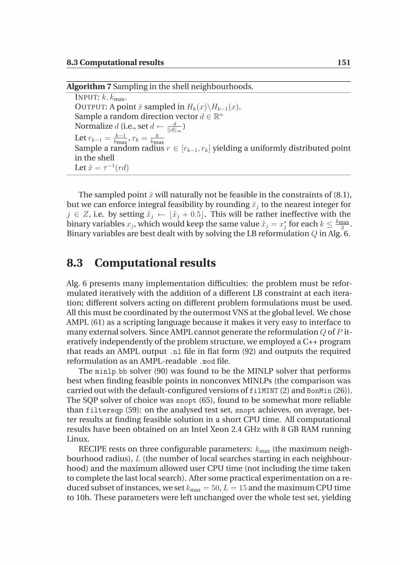
8.3 Computational results 151
Algorithm 7 Sampling in the shell neighbourhoods.
INPUT: k, kmax.OUTPUT: A point x sampled in Hk(x)\Hk−1(x).Sample a random direction vector d ∈ R
n
Normalize d (i.e., set d← d||d||∞
)
Let rk−1 = k−1kmax
, rk = kkmax
Sample a random radius r ∈ [rk−1, rk] yielding a uniformly distributed pointin the shellLet x = τ−1(rd)
The sampled point x will naturally not be feasible in the constraints of (8.1),but we can enforce integral feasibility by rounding xj to the nearest integer forj ∈ Z, i.e. by setting xj ← ⌊xj + 0.5⌋. This will be rather ineffective with thebinary variables xj , which would keep the same value xj = x∗j for each k ≤ kmax
2.
Binary variables are best dealt with by solving the LB reformulation Q in Alg. 6.
8.3 Computational results
Alg. 6 presents many implementation difficulties: the problem must be refor-mulated iteratively with the addition of a different LB constraint at each itera-tion; different solvers acting on different problem formulations must be used.All this must be coordinated by the outermost VNS at the global level. We choseAMPL (61) as a scripting language because it makes it very easy to interface tomany external solvers. Since AMPL cannot generate the reformulation Q of P it-eratively independently of the problem structure, we employed a C++ programthat reads an AMPL output .nl file in flat form (92) and outputs the requiredreformulation as an AMPL-readable .mod file.
The minlp bb solver (90) was found to be the MINLP solver that performsbest when finding feasible points in nonconvex MINLPs (the comparison wascarried out with the default-configured versions of filMINT (2) and BonMin (26)).The SQP solver of choice was snopt (65), found to be somewhat more reliablethan filtersqp (59): on the analysed test set, snopt achieves, on average, bet-ter results at finding feasible solution in a short CPU time. All computationalresults have been obtained on an Intel Xeon 2.4 GHz with 8 GB RAM runningLinux.
RECIPE rests on three configurable parameters: kmax (the maximum neigh-bourhood radius), L (the number of local searches starting in each neighbour-hood) and the maximum allowed user CPU time (not including the time takento complete the last local search). After some practical experimentation on a re-duced subset of instances, we set kmax = 50, L = 15 and the maximum CPU timeto 10h. These parameters were left unchanged over the whole test set, yielding

152 A Good Recipe for Solving MINLPs
good results without the need for fine-tuning.
8.3.1 MINLPLib
The MINLPLib (30) is a collection of Mixed Integer Nonlinear Programmingmodels which can be searched and downloaded for free. Statistics for the in-stances in the MINLPLib are available from:
http://www.gamsworld.org/minlp/minlplib/minlpstat.htm.
The instance library is available at:
http://www.gamsworld.org/minlp/minlplib.htm.
The MINLPLib is distributed in GAMS (28) format, so we employed an auto-matic translator to cast the files in AMPL format.
At the time of downloading (Feb. 2008), the MINLPLib consisted of 265 MINLPinstances contributed by the scientific and industrial OR community. Thesewere all tested with the RECIPE algorithm implementation described above.We had 20 unsuccessful runs due to some AMPL-related errors (the model con-tained some unusual AMPL operator not implemented by some of the solversor reformulators employed in RECIPE). The instances leading to AMPL-relatedfailure were:
blendgap, dosemin2d, dosemin3d, fuzzy, hda, meanvarxsc, pb302035,pb302055, pb302075, pb302095, pb351535, pb351555, pb351575, pb351595,water3, waterful2, watersbp, waters, watersym1, watersym2.
The performance of RECIPE was evaluated on the 245 runs that came tocompletion. The results are given in Tables 8.1, 8.2 (solved instances) and 8.3(unsolved instances). Table 8.1 lists results where the best solution found byRECIPE was different by at least 0.1% from that listed in MINLPLib. The firstcolumn contains the instance name, the second contains the value f ∗ of the ob-jective function found by the RECIPE algorithm and the third the correspond-ing CPU usage measured in seconds of user time; the fourth contains the valuef of the objective function reported in the official MINLPLib table and the fifthcontains the name of corresponding GAMS solver that found the solution. Thefourth and fifth columns were generated using the data available from the MINLPLibwebsite, updated with some improved results obtained by AlphaECP (137) thatare not yet listed on the MINLPLib web page. Table 8.2 lists instance nameswhere the best values found by RECIPE and listed in MINLPLib are identical.
Instance RECIPE Known solutionf∗ CPU f Solver
csched2a -165398.701331 75.957500 -160037.701300 BonMineniplac -131926.917119 113.761000 -132117.083000 SBB+CONOPTex1233 160448.638212 3.426480 155010.671300 SBB+CONOPT

8.3 Computational results 153
Instance RECIPE Known solutionf∗ CPU f Solver
ex1243 118489.866394 5.329190 83402.506400 BARONex1244 211313.560000 7.548850 82042.905200 SBB+CONOPTex1265a 15.100000 9.644530 10.300000 BARONex3 -53.990210 1.813720 68.009700 SBB+CONOPTex3pb -53.990210 1.790730 68.009700 SBB+CONOPTfo7 2 22.833307 23.710400 17.748900 AlphaECPfo7 24.311289 25.423100 20.729700 AlphaECPfo9 38.500000 46.296000 23.426300 AlphaECPfuel 17175.000000 1.161820 8566.119000 SBB+CONOPTgear4 1.968201 9.524550 1.643400 SBB+CONOPT2lop97ic 4814.451760 3047.110000 4284.590500 -lop97icx 4222.273030 1291.510000 4326.147700 SBB+CONOPTm7 220.530055 17.275400 106.756900 AlphaECPminlphix 209.149396∗ 4.849260 316.692700 SBB+snoptnuclear14b -1.119531 7479.710000 -1.113500 SBB+CONOPTnuclear24b -1.119531 7483.530000 -1.113500 SBB+CONOPTnuclear25 -1.120175 1329.530000 -1.118600 SBB+CONOPTnuclearva -1.008822 167.102000 -1.012500 SBB+CONOPT2+snoptnuclearvb -1.028122 155.513000 -1.030400 SBB+CONOPT2+snoptnuclearvc -1.000754 176.075000 -0.998300 SBB+CONOPT2+snoptnuclearvd -1.033279 202.416000 -1.028500 SBB+CONOPT2+snoptnuclearve -1.031364 193.764000 -1.035100 SBB+CONOPT2+snoptnuclearvf -1.020808 200.154000 -1.017700 SBB+CONOPT2+snoptnvs02 5.964189 1.925710 5.984600 SBB+CONOPT3nvs05 28.433982 4.215360 5.470900 SBB+CONOPT3nvs14 -40358.114150 2.070690 -40153.723700 SBB+CONOPT3nvs22 28.947660 4.849260 6.058200 SBB+CONOPT3o7 2 125.907318 23.262500 116.945900 AlphaECPo7 160.218617 24.267300 131.649300 AlphaECPoil -0.006926 389.266000 -0.932500 SBB+CONOPT(fail)product -1971.757941 2952.160000 -2142.948100 DICOPT+CONOPT3/CPLEX
st e13 2.236072 0.548916 2.000000 BARONst e40 52.970520 0.930858 30.414200 BARONstockcycle 120637.913333 17403.200000 119948.688300 SBB+CONOPTsuper3t -0.674621 38185.500000 -0.685965 SBB+CONOPTsynheat 186347.748738 3.534460 154997.334900 SBB+CONOPTtln7 19.300000 1000.640000 15.000000 BARONrisk2b −∞∗ 45.559100 -55.876100 SBB+CONOPT3risk2bpb −∞∗ 48.057700 -55.876100 SBB+CONOPT3
Table 8.1: Computational results on MINLPLib. Values denoted by ∗
mark instances with unbounded values in the solution.
alan ex1224 gbd nvs06 parallel st e32 tln2
batchdes ex1225 gear2 nvs07 prob02 st e36 tln4
batch ex1226 gear3 nvs08 prob03 st e38 tln5
cecil 13 ex1252a gear nvs09 prob10 st miqp1 tln6
contvar ex1252 gkocis nvs10 procsel st miqp2 tloss
csched1a ex1263a hmittelman nvs11 pump st miqp3 tls2
csched1 ex1263 johnall nvs12 qap st miqp4 util
csched2 ex1264a m3 nvs13 ravem st miqp5
du-opt5 ex1264 m6 nvs15 ravempb st test1
du-opt ex1265 meanvarx nvs16 sep1 st test2
enpro48 ex1266a nuclear14a nvs17 space25a st test3
enpro48pb ex1266 nuclear14 nvs18 space25 st test4
enpro56 ex4 nuclear24a nvs19 spectra2 st test6
enpro56pb fac1 nuclear24 nvs20 spring st test8
ex1221 fac2 nuclear25a nvs21 st e14 st testgr1
ex1222 fac3 nuclear25b nvs23 st e15 st testph4
ex1223a feedtray2 nvs01 nvs24 st e27 synthes1

154 A Good Recipe for Solving MINLPs
ex1223b feedtray nvs04 oaer st e29 synthes2
ex1223 gastrans nvs03 oil2 st e31 synthes3
Table 8.2: Instances for which RECIPE’s optima are the same as thosereported in the MINLPLib.
8.3.2 Optimality
RECIPE found feasible solutions for 163 instances out of 245 (66%). Relative tothis reduced instance set, it found the best known solution for 121 instances(74%), gave evidence of the unboundedness of 3 instances (1%), and improvedthe best known objective value for 12 instances (7%). In the other cases it founda local optimum that was worse than the best known solution.
Improved solutions were found for the following instances:
csched2a: f ∗ = −165398.701331 (best known solution: −160037.701300)ex3: f ∗ = −53.990210 (best known solution: 68.009700)ex3pb: f ∗ = −53.990210 (best known solution: 68.009700)lop97icx: f ∗ = 4222.273030 (best known solution: 4326.147700)minlphix: f ∗ = 209.149396 (best known solution: 316.692700)nuclear14b: f ∗ = −1.119531 (best known solution: −1.113500)nuclear24b: f ∗ = −1.119531 (best known solution: −1.113500)nuclear25: f ∗ = −1.120175 (best known solution: −1.118600)nuclearvc: f ∗ = −1.000754 (best known solution: −0.998300)nuclearvd: f ∗ = −1.033279 (best known solution: −1.028500)nuclearvf: f ∗ = −1.020808 (best known solution: −1.017700)nvs02: f ∗ = 5.964189 (best known solution: 5.984600)nvs14: f ∗ = −40358.114150 (best known solution: −40153.723700)risk2b: f ∗ = −∞ (best known solution: −55.876100)risk2bpb: f ∗ = −∞ (best known solution: −55.876100).
All new best solutions were double-checked for constraint, bounds and in-tegrality feasibility besides the verifications provided by the local solvers, andwere all found to be integral feasible; 11 out of 12 were constraint/bound feasi-ble to within a 10−5 absolute tolerance, and 1 (csched2a) to within 10−2. The 3instances marked by ∗ in Table 8.1 (minlphix, risk2b, risk2bpb) gave solutionsx∗ with some of the components at values in excess of 1018. Since minlphix min-imizes a fractional objective function and there are no upper bounds on severalof the problem variables, the optimum is attained when the variables appear-ing in the denominators tend towards +∞. We solved risk2b and risk2bpb sev-eral times, setting increasing upper bounds to the unbounded variables: thisyielded decreasing values of the objective function, suggesting that these in-stances are really unbounded (hence the−∞ in Table 8.1).

8.3 Computational results 155
4stufen eg int s fo8 ar4 1 m7 ar4 1 nuclear10a o9 ar4 1 super3 waste
beuster elf fo8 ar5 1 m7 ar5 1 nuclear10b ortez tln12 water4
deb10 fo7 ar2 1 fo9 ar2 1 mbtd nuclear49 product2 tls12 waterx
deb6 fo7 ar25 1 fo9 ar25 1 no7 ar2 1 nuclear49a qapw tls4 waterz
deb7 fo7 ar3 1 fo9 ar3 1 no7 ar25 1 nuclear49b saa 2 tls5 windfac
deb8 fo7 ar4 1 fo9 ar4 1 no7 ar3 1 o7 ar2 1 space960 tls6
deb9 fo7 ar5 1 fo9 ar5 1 no7 ar4 1 o7 ar25 1 st e35 tls7
detf1 fo8 gasnet no7 ar5 1 o7 ar3 1 st test5 tltr
eg all s fo8 ar2 1 m7 ar2 1 nous1 o7 ar4 1 st testgr3 uselinear
eg disc2 s fo8 ar25 1 m7 ar25 1 nous2 o7 ar5 1 super1 var con10
eg disc s fo8 ar3 1 m7 ar3 1 nuclear104 o8 ar4 1 super2 var con5
Table 8.3: Instances unsolved by RECIPE.
On 82 instances out of 245 listed in Table 8.3, RECIPE failed to find any localoptimum within the allotted time limit. Most of these failures are due to the dif-ficulty of the continuous relaxation of the MINLPs: there are several instanceswhere the SQP method (snopt) does not manage to find a feasible starting point,and in these cases the convex MINLP solver (minlp bb) also fails. On a smallernumber of instances, minlp bb is not able to find integral feasible solutions eventhough constraint feasible solutions are provided by snopt.
8.3.3 Reliability
One interesting feature of RECIPE is its reliability: in its default configurationit managed to find solution with better or equal quality than those reportedin the MINLPLib on 136 instances over 245 (55%) and at least a feasible pointin a further 11% of the cases. On the same set of test instances, the closestcompetitor is SBB+CONOPT, which matches or surpasses the best solutions inMINLPLib in 37% of the cases, followed by BARON with 15% and by AlphaECPwith 14%. These percentages were compiled in June 2008 by looking at:
http://www.gamsworld.org/minlp/minlplib/points.htm.
8.3.4 Speed
The total time taken for solving the whole MINLPLib (including the unsolvedinstances, where the VNS algorithm terminates after exploring the neighbour-hoods up to kmax or when reaching the 10 hours time limit, whichever comesfirst) is roughly 4 days and 19 hours of user CPU time. RECIPE’s speed is verycompetitive with that of sBB approaches: tests conduced using the ooOPS solver(91; 92; 100) as well as BARON on some complex MINLPs showed that sBB meth-ods may take a long time to converge. Naturally, the trade-off for this speed isthe lack of an optimality guarantee.

156 A Good Recipe for Solving MINLPs

Chapter 9
Computational Experiments on theTDSPP
Throughout this part, we tested our methods on common benchmark instancestaken from the literature, so that we could compare with other works. We nowrevert our attention back to the time-dependent shortest paths problem. In thischapter we test the most efficient algorithms proposed so far on shortest pathinstances, using a combination of real-world and synthetic data.
The rest of this chapter is organized as follows. In Section 9.1 we discussthe input data for our numerical tests. In Section 9.2 we test the linear formula-tion of the TDSPP with a Branch-and-Bound algorithm which uses the branch-ing rules proposed in Chapter 7. In Section 9.3 we apply the VNS algorithm ofChapter 8 to the MINLP formulation of the TDSPP.
9.1 Input data
For our numerical experiments, we extracted several subnetworks of increasingsize from the road network of Rome. The original graph is available from theweb page of the 9th DIMACS Challenge – Shortest Paths:
http://www.dis.uniroma1.it/~challenge9/.
There are 3353 vertices and 8870 oriented arcs in the road network; however,our formulation (GTDSPP ) contains one (integer) variable for each arc andtwo variables for each node of the graph, as well as additional variables neededto model arc costs. Therefore, to keep computational times down to acceptablelevels, we considered subnetworks extracted from this graph instead of the fullsize graph. In particular, we tested our methods on networks with the charac-teristics reported in Table 9.1. Due to the large number of variables and con-straints that arise in the formulations (both linear and nonlinear), we were notable to carry out computational experiments in reasonable time on instanceswith more arcs and nodes than those reported in Table 9.1.

158 Computational Experiments on the TDSPP
NAME NODES ARCS
R-8 8 14R-30 30 62R-60 60 144
R-120 120 296R-200 200 504
Table 9.1: Size of the test instances.
Time-dependent costs were generated following some simple guidelines. Forpiecewise linear cost functions, we considered 3 breakpoints on each arc. Al-though this may seem like a small number, the trouble lies in the fact that eachbreakpoint introduces additional variables. Moreover, our approach is basedon the consideration that, instead of assigning to each arc a cost profile for afull day and using a nonzero departure times for each shortest path computa-tion, we can consider the departure time to be always zero and “shift” the costprofiles accordingly. That is, the 3 breakpoints can be considered as the first 3breakpoints on the cost profile after the desired departure time. If the time hori-zon covered by the 3 breakpoints is sufficiently large, this approach is equiva-lent to considering the full cost profiles, but requires significantly less effort.Breakpoints were positioned randomly within a time horizon of 3 hours, andtheir value for arc (u, v) was selected uniformly at random in [λ(u, v), 20λ(u, v)],where, as usual, λ(u, v) is the travelling time over (u, v) in traffic free situation.Note that we did not enforce the FIFO property when generating arc costs.
For the nonlinear model, we used the cost functions proposed in Section1.2.2 involving a summation of Gaussians. We set the number of cost perturba-tions to two, i.e. each cost function is of the form
c(i, j, τ) = cij +2
∑
k=1
ake−
(τ−µk)2
2σ2k ,
We used the same idea of “shifting” cost profiles described above. Therefore,the departure time of each shortest path is considered to be always zero, andthe cost perturbations that correspond to traffic jams are centered within atime horizon of 3 hours. The mean µk for each gaussian is picked uniformlyat random in the time interval between 0 and 3 hours (rounding to the nearestsecond), whereas the standard deviation σk is always 900 (we remark that timeis expressed in seconds). Each Gaussian function on arc (u, v) is multiplied bya factor ak that is chosen uniformly between [λ(u, v), 20λ(u, v)].

9.2 Numerical experiments with the linear formulation 159
9.2 Numerical experiments with the linear
formulation
In this section we discuss the computational experiments carried out on theMILP formulation for the TDSPP. First, we give more details on the formulation;then, we analyse the computational results.
9.2.1 Formulation
Consider the formulation (GTDSPP ) presented in Section 1.3:
min τt
∀v ∈ V∑
(i,j)∈A mvijxij = bv
∀v ∈ V τv ≤ dv
∀(i, j) ∈ A xij(di + c(i, j, di)) ≤ τj
∀(i, j) ∈ A xij ∈ {0, 1}∀v ∈ V τi ≥ 0
(GTDSPP )
In this section, we consider c(i, j, di) to be a piecewise linear function for all arcs(i, j) ∈ A. We are given a set of breakpoint positions brpk
ij, k = 1, . . . , h and a setof corresponding breakpoint values brvk
ij, k = 1, . . . , h for each arc (i, j). We addbinary variables δk
ij that select which piece of the piecewise linear function on(i, j) is active for a given departure time τi from node i. Note that, for simplicity,we considered each arc cost function expressed as a sum between a fixed (static)cost cij and a piecewise linear function, described as above. This way, for alltime instants following the last breakpoint brph
ij , the cost of an arc is given by itsfixed cost only. Therefore, the formulation becomes:
min τt
∀v ∈ V∑
(i,j)∈A mvijxij = bv
∀v ∈ V τv ≤ dv
∀(i, j) ∈ A xij(di + cij
∑h−1k=1 δk
ij(di−brpk
ij
brpk+1ij −brpk
ij
(brvk+1ij − brvk
ij) + brvkij)) ≤ τj
∀(i, j) ∈ A∑h−1
k=1 δkijbrp
kij + δh
ijM ≥ di
∀(i, j) ∈ A∑h
k=2 δkijbrp
k−1ij ≤ di
∀(i, j) ∈ A∑h
k=1 δkij = 1
∀(i, j) ∈ A xij ∈ {0, 1}∀(i, j) ∈ A δk
ij ∈ {0, 1}∀v ∈ V τi ≥ 0.
The third constraint is the complicating one: it involves the product betweena binary variable and a continuous variable, and between two binary variablesand a continuous variable. All these products can be formulated exactly withlinear terms, introducing additional variables (see e.g. (94)).

160 Computational Experiments on the TDSPP
The resulting MILP has a weak LP relaxation, due to the product reformula-tions which are known to be weak. Therefore, solving large instances to provenoptimality is a very difficult task. However, our aim is to compare on this classof problems traditional branching rules with the methods studied in this thesis.We note that, if no path between the source node and the target node exists,then this is detected at root node, since the LP relaxation is infeasible becauseof the flow conservation constraints.
9.2.2 Computational results
In Table 9.2 we report the number of variables and of constraints for all test in-stances with the MILP formulation described Section 9.2.1, before preprocess-ing. Although the number of variables and constraints is large, the constraintmatrix is sparse, hence the number of nonzeroes is small; this is because theflow conservation constraints have only two nonzeroes per row. Note that thesize of the formulation grows rapidly with the size of the network; a great deal ofthis growth is due to the complexity of modeling the arc cost functions, whichrequires several variables and constraints for each arc of the network.
NAME # VARIABLES # CONSTRAINTS
R-8 142 282R-30 618 1238R-60 1342 2780
R-120 2734 5666R-200 4396 9976
Table 9.2: Number of variables and of constraints of the MILP formu-lation for the TDSPP.
The setup for numerical experiments is as follows: we compare the CGD andSD branching algorithms discussed in Chapter 7 on the instances described inSection 9.1. For each instance, we selected 100 unique source/target pairs atrandom, and used our implementations of CGD and SD. For the smallest in-stance (R-8), instead of selecting 100 source/target pairs at random, we testedall possible source/target pairs. We allow Cplex’s cutting planes and preprocess-ing at root node, with default parameters; time limit is set to two hours, whereasthere is no limit on the number of nodes. Since the value of the optimum is notknown in advance, heuristics were not disabled, in contrast to the experimentsin Chapter 7.
We report, for each instance, average values over all the shortest paths com-putations. Source/destination pairs that are solved in less than two nodes byboth methods are not considered when computing the averages. We report thefollowing values (in the order in which they appear as columns):

9.2 Numerical experiments with the linear formulation 161
• percentage of instances solved to optimality by SD within the two hourstime limit;
• percentage of instances solved to optimality by CGD within the two hourstime limit;
• average number of nodes enumerated by SD on instances which are solvedby both methods;
• average CPU time (in seconds) of SD on instances which are solved byboth methods;
• average number of nodes enumerated by CGD on instances which aresolved by both methods;
• average CPU time (in seconds) of CGD on instances which are solved byboth methods;
• average number of nodes enumerated by SD on instances which are un-solved by either method;
• average relative integrality gap left by SD on instances unsolved by eithermethod, computed as (ub−lb)/ub where ub is the best known upper bound(i.e. primal feasible solution) and lb the best known lower bound after twohours;
• average number of nodes enumerated by CGD on instances which are un-solved by either method;
• average relative integrality gap left by CGD on instances unsolved by ei-ther method, computed as (ub − lb)/ub where ub is the best known upperbound and lb the best known lower bound after two hours.
All averages are geometric, computed as in Section 7.4. Note that, since wedo not known the optimal solution a priori, we record the amount of relativeintegrality gap left, i.e. not closed; therefore, optimality is attained when thisvalue becomes 0%. On all instances, Cplex’s heuristics were able to find at leastone feasible solution. The first feasible solution is typically discovered at rootnode in almost all cases.
Table 9.3 shows that CGD consistently performs better than SD on average.On the smallest road network (R-8), all shortest path computations are solvedto optimality at root node; therefore, CGD and SD perform equally. As the sizeof the road network increases, which corresponds to a larger number of vari-ables and constraints, CGD closes a larger amount of gap per node. Instanceswhich are solved by both methods require fewer nodes and less CPU time onaverage when employing our improved branching strategy CGD; similarly, on

162 Computational Experiments on the TDSPP
NUM. SOLVED UNSOLVED
SOLVED SD CGD SD CGD
SD CGD nodes time nodes time nodes gap nodes gap
R-8 100% 100% 0 0.02 0 0.02 - - - -
R-30 98% 93% 2508 345.95 80 34.15 - - - -
R-60 55% 60% 845 82.95 74 22.75 57133 87.7% 30792 70.4%
R-120 40% 40% 317 62.39 53 48.50 23991 83.6% 13405 75.8%
R-200 23% 42% 1349 701.08 378 433.46 8599 97.4% 4385 93.7%
Table 9.3: Comparison of the SD and CGD branching algorithms onthe MILP formulation for the time-dependent shortest paths problem.
instances which are unsolved by either method we close a larger integrality gap,even though we enumerate fewer nodes in the 2 hours time limit. Althoughit may look counterintuitive that the number of nodes (and CPU time for un-solved instances) decreases as the size of the instance increases, this dependson the way the average values are computed. In fact, results are computed oninstances that are solved by both methods, and on instances that are unsolvedby either method. As the size of the instances grows, only very easy shortestpath computations are carried out to optimality; therefore, there is a decreasein the number of nodes required on average on solved instances, but the num-ber of such instances also decreases (which can be seen in the second and thirdcolumn). Similarly, we enumerate fewer nodes in two hours on the unsolvedinstances, because the LP relaxation becomes more expensive. We note that,for moderate size instances already, not all shortest path computations can becarried out to optimality within the time limit; this is due to the large numberof variables and constaints, and to the weakness of the LP relaxation, whichmakes increasing the lower bound very difficult. In order to deal with full city-sized road networks, it would probably be necessary to give up some accuracyin the network modeling, so as to have a manageable number of variables andconstraints. However, the most effective branching strategy proposed in Chap-ter 7 shows an improvement over traditional branching rules on shortest pathinstances too, assessing its practical usefulness.
9.3 Numerical experiments with the nonlinear
formulation
In this section we discuss the computational experiments carried out on theMINLP formulation for the TDSPP. As for the linear case, we give more detailson the formulation; then, we discuss the modifications that we applied to theRECIPE algorithm (Chapter 8) to increase its performance on this particularkind of problems. Finally, we present computational results.
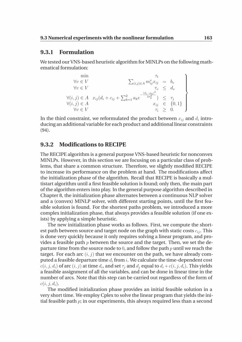
9.3 Numerical experiments with the nonlinear formulation 163
9.3.1 Formulation
We tested our VNS-based heuristic algorithm for MINLPs on the following math-ematical formulation:
min τt
∀v ∈ V∑
(i,j)∈A mvijxij = bv
∀v ∈ V τv ≤ dv
∀(i, j) ∈ A xij(di + cij +∑2
k=1 ake−
(di−µk)2
2σ2k ) ≤ τj
∀(i, j) ∈ A xij ∈ {0, 1}∀v ∈ V τi ≥ 0.
In the third constraint, we reformulated the product between xij and di intro-ducing an additional variable for each product and additional linear constraints(94).
9.3.2 Modifications to RECIPE
The RECIPE algorithm is a general purpose VNS-based heuristic for nonconvexMINLPs. However, in this section we are focusing on a particular class of prob-lems, that share a common structure. Therefore, we slightly modified RECIPEto increase its performance on the problem at hand. The modifications affectthe initialization phase of the algorithm. Recall that RECIPE is basically a mul-tistart algorithm until a first feasible solution is found; only then, the main partof the algorithm enters into play. In the general purpose algorithm described inChapter 8, the initialization phase alternates between a continuous NLP solverand a (convex) MINLP solver, with different starting points, until the first fea-sible solution is found. For the shortest paths problem, we introduced a morecomplex initialization phase, that always provides a feasible solution (if one ex-ists) by applying a simple heuristic.
The new initialization phase works as follows. First, we compute the short-est path between source and target node on the graph with static costs cij . Thisis done very quickly because it only requires solving a linear program, and pro-vides a feasible path p between the source and the target. Then, we set the de-parture time from the source node to 0, and follow the path p until we reach thetarget. For each arc (i, j) that we encounter on the path, we have already com-puted a feasible departure time di from i. We calculate the time-dependent costc(i, j, di) of arc (i, j) at time di, and set τj and dj equal to di + c(i, j, di). This yieldsa feasible assignment of all the variables, and can be done in linear time in thenumber of arcs. Note that this step can be carried out regardless of the form ofc(i, j, di).
The modified initialization phase provides an initial feasible solution in avery short time. We employ Cplex to solve the linear program that yields the ini-tial feasible path p; in our experiments, this always required less than a second

164 Computational Experiments on the TDSPP
of CPU time. Although the solution that we compute through this heuristic maybe far from the optimum, it still provides a starting point for our VNS-based al-gorithm. An additional advantage is that we are able to detect immediately ifthere is no path between the source and the destination node, i.e. if no feasiblesolution exists.
9.3.3 Computational results
Numerical experiments were run as follows: for each instance described in Sec-tion 9.1, we generated 100 distinct source/destination pairs at random, and em-ployed the RECIPE algorithm that is discussed in Chapter 8 with the modifica-tions presented in Section 9.3.2. For the smallest instance (R-8), instead of se-lecting 100 source/target pairs at random, we tested all possible source/targetpairs.
We ran some preliminary tests with different solvers employed on this for-mulation within RECIPE (minlp bb and bonmin (26)), as well as the exact Branch-and-Bound solver couenne for nonconvex MINLPs (see (23; 22)). All these solversexperienced severe numerical difficulties due to the summation of Gaussianfunctions, which turned out to be very difficult to treat: in several cases, the con-tinuous relaxation of the problem is not solved to feasibility by the NLP solversemployed within minlp bb, bonmin and couenne, even though a feasible solutionexists. Therefore, we decided to replace each Gaussian function G(µk, σk) withits Taylor series up to the fourth term, centered at µk, for all time instants lessthan 3σk away from the mean. The contribution of each Gaussian was consid-ered to be zero for τ ∈ T : |τ − µk| ≥ 3σk. To truncate the power series, we useda binary variable for each Gaussian term, which indicates whether the functionis active or not. Note that the feasibility heuristic described in Section 9.3.2 canstill be applied: we compute a feasible assignment of the binary variables thatdetermine whether a Gaussian function on arc (i, j) is active or not (depend-ing on the departure time di from node i), then we compute the cost of the arcdefined through the Taylor series.
In Table 9.4 we report the number of variables and of constraints for alltest instances with the MINLP formulation described above, before preprocess-ing. Again, the flow conservation constraints have only two nonzeroes per row,therefore part of the constraint matrix is very sparse. We were not able to solveinstances larger than R-60 in a reasonable amount of time; in particular, theconvex MINLP solver minlp bb employed during the local search phase by ourRECIPE algorithm is not able to provide a solution within the 3 hours timelimit for instances larger than R-60. The same applies to couenne, whose pri-mal heuristics fail due to the size of the problem, and no feasible solution isfound within the time limit.
Since the NLP relaxations encountered during the solution process are ex-pensive, and we did not want to invest too much time on each shortest path
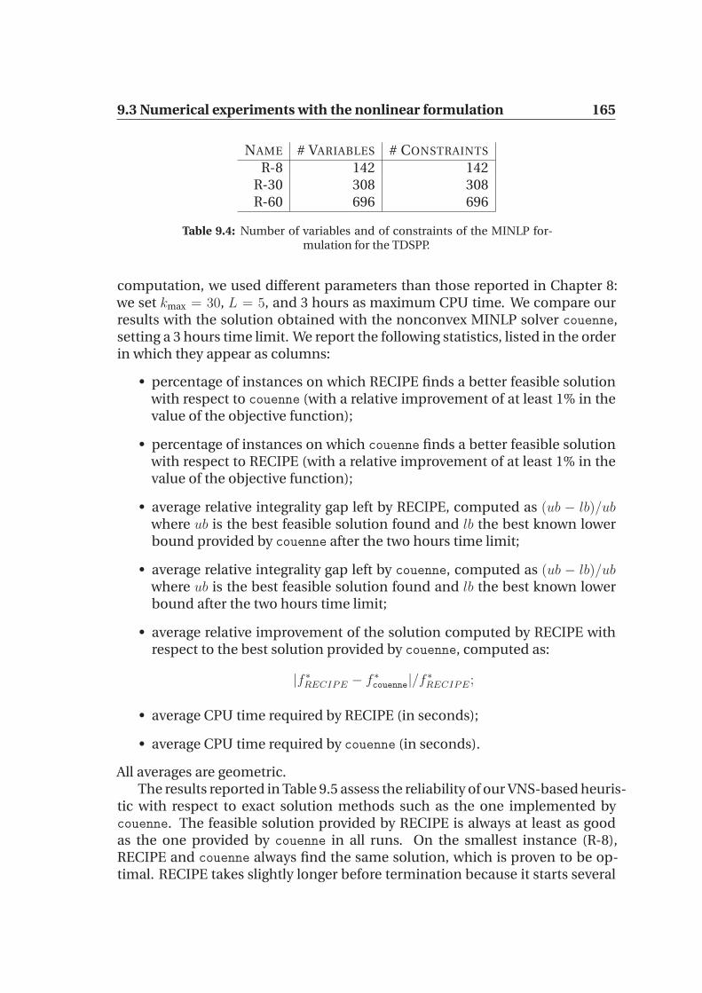
9.3 Numerical experiments with the nonlinear formulation 165
NAME # VARIABLES # CONSTRAINTS
R-8 142 142R-30 308 308R-60 696 696
Table 9.4: Number of variables and of constraints of the MINLP for-mulation for the TDSPP.
computation, we used different parameters than those reported in Chapter 8:we set kmax = 30, L = 5, and 3 hours as maximum CPU time. We compare ourresults with the solution obtained with the nonconvex MINLP solver couenne,setting a 3 hours time limit. We report the following statistics, listed in the orderin which they appear as columns:
• percentage of instances on which RECIPE finds a better feasible solutionwith respect to couenne (with a relative improvement of at least 1% in thevalue of the objective function);
• percentage of instances on which couenne finds a better feasible solutionwith respect to RECIPE (with a relative improvement of at least 1% in thevalue of the objective function);
• average relative integrality gap left by RECIPE, computed as (ub − lb)/ubwhere ub is the best feasible solution found and lb the best known lowerbound provided by couenne after the two hours time limit;
• average relative integrality gap left by couenne, computed as (ub − lb)/ubwhere ub is the best feasible solution found and lb the best known lowerbound after the two hours time limit;
• average relative improvement of the solution computed by RECIPE withrespect to the best solution provided by couenne, computed as:
|f ∗RECIPE − f ∗couenne|/f∗RECIPE;
• average CPU time required by RECIPE (in seconds);
• average CPU time required by couenne (in seconds).
All averages are geometric.The results reported in Table 9.5 assess the reliability of our VNS-based heuris-
tic with respect to exact solution methods such as the one implemented bycouenne. The feasible solution provided by RECIPE is always at least as goodas the one provided by couenne in all runs. On the smallest instance (R-8),RECIPE and couenne always find the same solution, which is proven to be op-timal. RECIPE takes slightly longer before termination because it starts several

166 Computational Experiments on the TDSPP
# BETTER SOL. INTEGRALITY GAP IMPR. CPU TIME
RECIPE couenne RECIPE couenne RECIPE couenne
R-8 0% 0% 0% 0.0% 0.0% 9.8 2.0
R-30 53% 0% 82.3% 88.4% 2.3% 6189.2 10848.6
R-60 80% 0% 99.5% 100.0% 28.5% 8514.0 10788.4
Table 9.5: Comparison of RECIPE and couenne on the MINLP formu-lation for the time-dependent shortest paths problem.
local searches, whereas couenne is able to prove optimality in a very short time.Overall, on such a small instance using an exact method such as couenne seemslike a better option, because we have a guarantee of optimality and runningtimes are short. However, if we increase the size of the underlying road net-work, then RECIPE becomes more appealing with respect to couenne: on aver-age, the solution quality increases by a factor that becomes larger as the size ofthe instances grows. Correspondigly, the amount of integrality not closed de-creases. Note that for the R-60 instance the amount of integrality gap left is al-most 100%, because on most instances couenne is not able to increase the lowerbound to a value larger than zero; but the improvement in the objective valueof the solution found by RECIPE with respect to couenne is significant. More-over, RECIPE is fast: on several instances, an application of RECIPE terminatesbefore the 3 hours time limit, whereas couenne hits the time limit on almost allinstances (which is shown by an average running time close to 3 hours). Sum-marizing, our heuristic algorithm performs on average very well on these short-est path instances, finding better solutions than the exact Branch-and-Boundsolver couenne within the allotted time frame; the only exception is given byvery small instances, where RECIPE and couenne always find the same optimalsolution, but couenne is slightly faster. Unfortunately, we were not able to ap-ply RECIPE to larger instances because of the failure of the local solvers whendealing with too many variables and constraints, but we have no reasons to be-lieve that RECIPE would not scale well if the local solvers were able to deal withlarger problem sizes.

Part III
Conclusions and Bibliography


Chapter 10
Summary and Future Research
10.1 Summary
We considered the problem of finding the shortest path between two nodeson a large-scale time-dependent graph, which has many interesting practicalapplications. The problem is theoretically solved in an efficient way by Dijk-stra’s algorithm under the FIFO property, but there are many real-time applica-tions where employing Dijkstra’s algorithm would take too much time. Thus,we analysed speedup techniques for this algorithm. Moreover, we proposed amathematical programming formulation for the point-to-point shortest pathproblem, starting from a classical formulation for static graphs and modifyingit in order to take into account time-dependency in non-FIFO networks andpossibly nonlinear time-dependent cost functions. We analyzed the resultingformulation, which is a MILP if the arc cost functions are linear or piecewise lin-ear, whereas it is a MINLP if they are arbitrary nonlinear functions. We studiedalgorithms for both classed of problems, and tested them on both benchmarkinstances taken from the literature and shortest path instances.
First, we reviewed existing speedup techniques, both for static graphs andfor time-dependent graphs. This allowed us to underline that the fastest al-gorithms typically rely on hierarchical approaches, sometimes combined withgoal directed search. However, hierarchical methods are inherently bidirec-tional, and bidirectional search cannot be directly applied on time-dependentgraphs. Therefore, we tried to overcome this problem. We discussed a methodbased on defining small node sets with an approximation guarantee; Dijkstrasearches are constrained to explore only nodes in these precomputed sets, hencethe number of touched nodes decreases. We analyzed advantages and draw-backs of this approach. We developed a general framework for bidirectionalsearch on time-dependent graphs; the main idea is to run a time-dependentforward search, and a time-independent backward search whose purpose isto bound the set of nodes explored by the forward search. Following this ap-proach, we are able to improve the efficacy of the ALT algorithm, which is a
170 Summary and Future Research
clever application of the well known A∗ algorithm to road networks; part ofthis improvement is due to the strengthening of the lower bounds to distanceswithin the graph which are used throughout the algorithm. We proved correct-ness of the proposed method, and also proposed several enhancements. Asa consequence, we were able to apply a two-levels hierarchical approach ontime-dependent graphs. This is based on the idea of selecting a small subnet-work which contains important arcs; then, most of the calculations are carriedout on the subnetwork, so that fewer nodes have to be explored. In analogywith the real world, this can be viewed as the motorway network, which is asubset of the original road network: when planning the route between two suffi-ciently distant points, local roads are considered only in a small radius centeredon the departure and the destination point, but most of the path relies on mo-torway segments. From a theoretical point of view, our two-levels hierarchicalapproach could be extended to a multi-level hierarchy. However, our compu-tational experiments, as well as numerical experiences reported in the litera-ture, suggest that multi-level hierarchies do not work well for time-dependentgraphs as they do for static graphs. Therefore, we only considered at most twolevels.
One of the advantages of our method is its straightforward extension to dy-namic scenarios, that is, scenarios where the cost functions on arcs are notfixed, but can be updated from time to time. This is a practical problem whichhas been previously described in the literature for the static case, but which hadnot been tackled in the time-dependent case. It turns out that we only need asmall computational overhead to restore optimality of the hierarchy wheneversome cost functions are updated. The amount of necessary work depends onthe number and the position of the updated arcs: our algorithm benefits fromspatial locality; therefore, if several contiguous arcs have their cost changed, wecan run the update in an efficient way. We remark that, for real world applica-tions, this is often the case: traffic jams typically extend over several adjacentroad segments.
We provided extensive computational experiments to show the effective-ness of our approach on real world data. We tested the algorithm on two differ-ent road networks: the road network of Western Europe with generated time-dependent data, which is commonly used as a benchmark in the literature, andthe road network of France with real world time-dependent data. We analysedthe performance of our algorithm taking into account different criteria, andcomparing with other existing methods. The main improvement of our ap-proach with respect to the existing algorithms is the significant reduction (twoorders of magnitude, if comparing to Dijkstra’s algorithm or unidirectional ALT)of the average number of settled nodes for a path computation, which leads toaverage query times of a few milliseconds. Only the recently developed SHARCalgorithm is faster than our method; however, SHARC cannot deal with the dy-namic scenario. Moreover, our method can also compute approximated solu-

10.1 Summary 171
tions, with approximation guarantee defined at query time; if we are willingto accept a maximum approximation of 5%, then our algorithm is faster thanSHARC. Optimality of the hierarchy after modifications in the cost functionscan be restored very quickly, if the algorithm is parameterized to do so; indeed,there is a trade off between query speed and update speed, which depends onthe values of the parameters for the preprocessing phase. We analysed the al-gorithm performance for several values of these parameters, so as to provideenough information to strike a good balance for real world applications.
We described a real world application: we integrated an implementation ofour algorithm in C++ within an existing industrial platform which collects, gath-ers and treats real-time traffic information and traffic forecasts. Our aim was toprovide a path computation service for the website of the Mediamobile com-pany, which deals with traffic information and, as such, required an algorithmcapable of answering several shortest path queries per second taking into ac-count the most recent available traffic forecasts. To this end, we proposed aleast squares algorithm to modify the arc cost functions, so as to fit the trafficforecasts as much as possible at each update.
Within the context of solving MILPs with Branch-and-Bound, we proposedtwo methods to generate good split disjunctions for branching: a heuristic ap-proach that solves a quadratic optimization problem, and a mathematical for-mulation that models the problem of finding a split disjunction closing a largegap at the current node. Computational experiments show that both methodsare able to close more gap with respect to the traditional branching rule, whichconsists in branching on a single variable with fractional value. We proposed acombination of the heuristic procedure based on a quadratic formulation withbranching on single variables, and showed that the resulting branching algo-rithm, which we called CGD, is very effective in practice. Indeed, on a largeset of test instances, CGD performs better than branching on single variablesonly, both in terms of size of the enumeration tree and in terms of computingtime. Moreover, we are able to solve one very difficult instance, which is typi-cally not solved by commercial software. We implemented a branching schemebased on the mathematical formulation that models the problem of finding asplit disjunction closing a large gap, and we tested it on several heterogeneousinstances. This method is indeed capable of closing more gap with respect tobranching on single variables on the majority of test instances, but it requiresconsiderably more time, which does not seem to be worth the extra effort. Ifcompared to the heuristic procedure based on a quadratic formulation, thisapproach seems to work better on the difficult instances, but the heuristic pro-cedure is significantly faster.
Finally, we described a heuristic approach to solving nonconvex MINLPs.Our method, called RECIPE, combines several existing exact, approximate andheuristic techniques: the global search phase is cohordinated by the VNS meta-heuristic, whereas the local search employs both continuous NLP and convex

172 Summary and Future Research
MINLP solvers, with a neighbourhood structure defined through hyperrectan-gles and local branching. This results in an algorithm that can successfully solvemany difficult MINLPs without hand-tuned parameter configuration. Such areliable solver would be particularly useful in industrial applications where theoptimum quality is of relative importance and the optimization layer is hiddenfrom user intervention and is therefore “just supposed to work”. Over a largecollection of benchmark instances taken from the literature, not only we findthe best known solution for the majority of the test problems, but in some caseswe improve over the best known objective value, while requiring very low com-putational times.
The mathematical programming formulation that we proposed for the time-dependent shortest paths problem on non-FIFO networks turned out to bevery challenging for MILP and MINLP solvers; one of the difficulties is givenby the large number of variables and constraints that arise in the formulationand are necessary to model arc costs. Computational experiments on short-est path instances showed that, on the MILP formulation, the branching rulesdiscussed in this thesis achieved good results, cutting down the number of re-quired nodes by a significant factor on average. CPU times also benefited fromthe proposed approach. Despite developing a specially tailored initializationphase for RECIPE on this particular kind of shortest paths instances, we couldonly solve the MINLP formulation on small networks; numerical troubles af-fect both our heuristic VNS-based algorithm and exact solvers for nonconvexMINLPs. On the instances that we were able to solve, RECIPE showed goodresults, finding near-optimal solutions for almost all instances in a short CPUtime.
Summarizing, we reviewed the most successfull algorithms for the point-to-point shortest path problem on static road networks, which rely on two dif-ferent approaches, often mixed together: goal directed search and hierarchi-cal routing. Our aim was to apply the same techniques on time-dependentroad networks. To do so, we improved an existing algorithm for goal directedsearch in the time-dependent case, and we developed a framework for bidi-rectional search, that allowed an easy generalization of hierarchical routing totime-dependent networks. Computational experiments confirmed the efficacyin practice of our ideas. Moreover, our algorithm is the first method which isable to deal in an efficient way with dynamic time-dependent scenarios, thatis, applications where the time-dependent arc cost functions are not fixed andknown a priori, while still yielding a speedup of more than two orders of mag-nitude with respect to Dijkstra’s algorithm. We proposed a mathematical pro-gramming formulation for the TDSPP. We studied improvements for the widelyused Branch-and-Bound algorithm for MILPs, resulting in an average reduc-tion of the number of enumerated nodes by a factor of two and an excellentperfomance on some well known hard instances. These improvements rely onthe selection of a branching decision which is different from the standard rule

10.2 Future research 173
of branching on a single variable. We presented a general purpose heuristic fornonconvex MINLPs, which combines several off-the-shelf components into aneffective and fast solver for this difficult class of problems. We tested the pro-posed approach on the mathematical formulation for the TDSPP, analyzing thecomputational results.
10.2 Future research
Even if the speed and versatility showed by the shortest paths algorithm pro-posed in this thesis should be sufficient for most practical applications, there isstill much room for research in the field. For some applications, it would be de-sirable to have very fast query times and no additional overhead when changingthe cost functions. Examples of this are route planners which use different costfunctions depending on the vehicle type that is querying the path computingservice. Although this seems an impossible challenge, it is still an interestingsubject of research, maybe assuming some restrictions on the cost functions tosimplify the problem. If the cost functions are similar, the SHARC algorithmdiscussed in Section 1.4.6 has showed promising result. Another interesting di-rection for future research is multicriteria optimization. Routing applicationsin general networks (not necessarily road networks) often have to deal with sev-eral objective functions that the user would like to minimize; e.g., travellingtime and number of connections for railway routing, or travelling time and mo-torway fees for road networks. How to formalize this problem is unclear. Someapproaches rely on finding all the Pareto optima, and let the user choose amongthem. However, computing all the Pareto optima is a difficult task, and couldgreatly benefit from speedup techniques. We believe that the techniques pre-sented in this thesis could be used as a building brick for efficient algorithmsin the multiobjective case. At the moment of finalizing this thesis, we are awarethat an extension of the SHARC algorithm shows very good preliminary results(42). The greatest drawbacks of SHARC are its long preprocessing time and thecapability of dealing with static scenarios only. It would be interesting to hy-bridize SHARC with the techniques proposed in this work, so as to be able toperform efficient multicriteria optimization on dynamic networks.
Concerning the computation of split disjunctions to be employed as branch-ing decisions in MILPs, one of the main questions which still has to answeredis: given a good disjunctions, is it more profitable to branch on it or to use it togenerate a cutting plane? So far, the answer is not clear, and the question pro-vides an interesting challenge to the integer programming community. Devis-ing fast and efficient heuristics to generate strong disjunctions is another fieldwhich is currently studied by several research groups. It is important to notethat at the moment it is not known how much benefit could be brought by a“perfect” branching strategy: for cutting planes, some studies have underlined
174 Summary and Future Research
that there is still a large gap between the performance obtained by commonlyimplemented cutting planes and the theoretically achievable maximum. But itis difficult to undertake the same study for branching decisions. It is known thata decrease of the number of nodes of at least a factor of two can be obtained bycarefully choosing a branching disjunction; if this result could be achieved witha very small computational effort, branching on general disjunctions wouldbecome interesting for commercial solvers as well. We believe that our workmoves some steps in that direction.
Finally, heuristic approaches to the solution of nonconvex MINLPs have thepotential to play an important role in the near future. Some very large problemscan probably be solved only through heuristics, but what is more interesting isthat Branch-and-Bound solvers for MINLPs are trying to reach a maturity levelsimilar to those for MILPs, and one of the main differences between the two isthe number of available primal heuristics. Obviously, obtaining good feasiblesolutions is critical for the performance of a Branch-and-Bound, and to this endcommercial MILP codes have sometimes tens of fast heuristics. This trend hasincreased in recent years, and nonconvex MINLP solvers should probably fol-low the same steps if they want to be perceived as reliable and effective as theirlinear counterparts. Our VNS algorithm could be used within a Branch-and-Bound solver as a primal heuristic. There is of course room for improvementin the algorithm itself. It would be desirable to be able to find a first feasiblesolution as soon as possible; currently, we rely on a convex Branch-and-Boundsolver used in a heuristic way to perform this task. The starting point providedto the solver determines the chances of finding such a solution. We believethat employing constraint programming techniques to round to the nearest in-teger as many fractional integer variables as possible, while still maintainingconstraint feasibility, could greatly help. We also plan to test different solversto evaluate performance as a stand-alone heuristic, and to reduce the numberof parameters of the algorithm; preliminary tests show that a different combi-nation of solvers through the main phase of the algorithm yields significantlybetter solution quality, although at the expense of a longer CPU time.

Acknowledgements
First of all, I want to thank Leo Liberti for giving me the possibility of workingon this thesis: he always encouraged me to try harder, and much of this workwould not have been done if it were not for him. I could not hope for a betteradvisor.
But he is not the only one who deserves credit. Philippe Baptiste, PhilippeGoudal and Daniel Krob played an important part in advising me, althoughwith different roles, and so did all the people I often worked with, especially:Benjamin Becquet, Gerard Cornuejols, Daniel Delling, Nenad Mladenovic, Do-minik Schultes. They made this thesis possible. I also want to thank everyoneat Mediamobile for always being helpful and friendly, and Tapio Westerlund forcarefully checking through some misprints on the MINLPLib website.
Last but not least, the only people I could always count on, despite manydifficulties: my family and my friends. I will not name each and every one ofyou, but you know who you are. Thanks for everything.

176

Disclaimer
Parts of this thesis have appeared, or are going to appear, in the following works:(38; 43; 44; 99; 109; 110; 111; 112; 113; 114). Copyright is held by the editors,where applicable.

178
References
[1] K. Aardal, R. E. Bixby, C. A. J. Hurkens, A. K. Lenstra, and J. W. Smeltink.Market split and basis reduction: Towards a solution of the Cornuejols-Dawande instances. INFORMS Journal on Computing, 12(3):192–202,2000.
[2] K. Abhishek, S. Leyffer, and J. Linderoth. Filmint: An outer-approximation based solver for nonlinear mixed-integer programs. Tech-nical Report ANL/MCS-P1374-0906, Argonne National Laboratory, 2007.
[3] C. Adjiman, I. Androulakis, and C. Floudas. Global optimization ofMINLP problems in process synthesis and design. Computers & Chem-ical Engineering, 21:S445–S450, 1997.
[4] R. Ahuja, T. Magnanti, and J. Orlin. Network flows: theory, algorithms,and applications. Prentice-Hall, Inc., Upper Saddle River, NJ, USA, 1993.
[5] R. Ahuja, J. Orlin, S. Pallottino, and M. Scutella. Dynamic shortest pathsminimizing travel times and costs. Networks, 41(4):197–205, 2003.
[6] M. Ajtai. The shortest vector problem in l2 is NP-hard for randomizedreductions. In Proceedings of the 30th Annual ACM Symposium on Theoryof Computing, Dallas, TX, 1998.
[7] Proceedings of the 8th Workshop on Algorithm Engineering and Experi-ments (ALENEX 06), Lecture Notes in Computer Science. Springer, 2006.
[8] K. Andersen, G. Cornuejols, and Y. Li. Reduce-and-split cuts: Improvingthe performance of mixed integer Gomory cuts. Management Science,51(11):1720–1732, 2005.
[9] M. Aouchiche, J. Bonnefoy, A. Fidahoussen, G. Caporossi, P. Hansen,L. Hiesse, J. Lachere, and A. Monhait. VNS for extremal graphs 14: TheAGX 2 system. In Liberti and Maculan (98), pages 281–308.
[10] E. Balas. Intersection cuts - a new type of cutting planes for integer pro-gramming. Operations Research, 19(1):19–39, 1971.

180 REFERENCES
[11] E. Balas. Disjunctive programming. Annals of Discrete Mathematics, 5:3–51, 1979.
[12] E. Balas, S. Ceria, and G. Cornuejols. Mixed 0-1 programming bylift-and-project in a branch-and-cut framework. Management Science,42(9):1229–1246, 1996.
[13] E. Balas and A. Saxena. Optimizing over the split closure. MathematicalProgramming, 113(2):219–240, 2008.
[14] C. Barrett, K. Bisset, M. Holzer, G. Konjevod, M. Marathe, and D. Wag-ner. Engineering label-constrained shortest-path algorithms. In AAIM’08: Proceedings of the 4th international conference on Algorithmic Aspectsin Information and Management, pages 27–37, Berlin, Heidelberg, 2008.Springer-Verlag.
[15] C. Barrett, R. Jacob, and M. Marathe. Formal language constrained pathproblems. SIAM Journal of computing, 30(3):809–837, 2001.
[16] H. Bast, S. Funke, P. Sanders, and D. Schultes. Fast routing in road net-works with transit nodes. Science, 316(5824):566, 2007.
[17] V. Batz, R. Geisberger, and P. Sanders. Time dependent contrac-tion hierarchies — basic algorithmic ideas. Technical report, Uni-versitat Karlsruhe (TH), 2008. Available from World Wide Web:http://arxiv.org/abs/0804.3947.
[18] R. Bauer and D. Delling. SHARC: Fast and Robust Unidirectional Rout-ing. In Proceedings of the 10th Workshop on Algorithm Engineering andExperiments (ALENEX 08), pages 13–26. SIAM, 2008.
[19] R. Bauer, D. Delling, P. Sanders, D. Schieferdecker, D. Schultes, andD. Wagner. Combining hierarchical and goal-directed speed-up tech-niques for dijkstra’s algorithm. In McGeoch (104), pages 303–318.
[20] M. S. Bazaraa and R. W. Langley. A dual shortest path algorithm. SIAMJournal on Applied Mathematics, 26(3):496–501, 1974.
[21] M. Beckmann, C. McGuire, and C. Winsten. Studies in the economics oftransportation. Technical Report RM-1488, RAND Corporation, 1955.
[22] P. Belotti. Couenne, an open-source solver for mixed-integer nonconvexproblems. In preparation.
[23] P. Belotti, J. Lee, L. Liberti, F. Margot, and A. Wacther. Branchingand bounds tightening techniques for non-convex MINLP. Techni-cal Report RC24620, IBM, 2008. Available from World Wide Web:http://www.optimization-online.org/DB_HTML/2008/08/2059.html.

REFERENCES 181
[24] P. Bonami, L. Biegler, A. Conn, G. Cornuejols, I. Grossmann, C. Laird,J. Lee, A. Lodi, F. Margot, N. Sawaya, and A. Wachter. An algorithmicframework for convex Mixed Integer Nonlinear Programs. Technical Re-port RC23771, IBM Corporation, 2005.
[25] P. Bonami, G. Cornuejols, A. Lodi, and F. Margot. A feasibility pump forMixed Integer Nonlinear Programs. Technical Report RC23862 (W0602-029), IBM Corporation, 2006.
[26] P. Bonami and J. Lee. BONMIN user’s manual. Technical report, IBM Corpo-ration, June 2007.
[27] J. Brimberg and N. Mladenovic. A variable neighbourhood algorithm forsolving the continuous location-allocation problem. Studies in LocationAnalysis, 10:1–12, 1996.
[28] A. Brook, D. Kendrick, and A. Meeraus. Gams, a user’s guide. ACMSIGNUM Newsletter, 23(3-4):10–11, 1988.
[29] L. Buriol, M. Resende, and M. Thorup. Speeding up dynamicshortest path algorithms. INFORMS Journal on Computing,accepted for publication. Available from World Wide Web:http://www.research.att.com/~mgcr/doc/dspa.pdf.
[30] M. R. Bussieck, A. S. Drud, and A. Meeraus. MINLPLib — a collection oftest models for Mixed-Integer Nonlinear Programming. INFORMS Jour-nal on Computing, 15(1), 2003.
[31] I. Chabini. Discrete dynamic shortest path problems in transportationapplications: complexity and algorithms with optimal run time. Trans-portation Research Records, 1645:170–175, 1998.
[32] I. Chabini and S. Lan. Adaptations of the A∗ algorithm for the compu-tation of fastest paths in deterministic discrete-time dynamic networks.IEEE Transactions on Intelligent Transportation Systems, 3(1):60–74, 2002.
[33] Coin-or branch-and-cut. Available from World Wide Web:https://projects.coin-or.org/Cbc.
[34] Coin-or cut generation library. Available from World Wide Web:https://projects.coin-or.org/Cgl.
[35] A. Consulting and Development. SBB Release Notes, 2002.
[36] K. Cooke and E. Halsey. The shortest route through a network with time-dependent internodal transit times. Journal of Mathematical Analysisand Applications, 14:493–498, 1966.
182 REFERENCES
[37] T. H. Cormen, C. E. Leiserson, R. L. Rivest, and C. Stein. Introduction toAlgorithms. MIT Press, second edition, 2001.
[38] G. Cornuejols, L. Liberti, and G. Nannicini. Improved strate-gies for branching on general disjunctions. Technical Report2071, Optimization Online, 2008. Available from World Wide Web:http://www.optimization-online.com.
[39] C. Daganzo. Reversibility of time-dependent shortest path prob-lem. Technical report, Institute of Transportation Studies, Univer-sity of California, Berkeley, 1998. Available from World Wide Web:http://repositories.cdlib.org/its/reports/UCB-ITS-RR-98-14.
[40] B. C. Dean. Continuous-time dynamic shortest path algorithms. Master’sthesis, Massachussets Institute of Technology, 1999.
[41] D. Delling. Time-Dependent SHARC-Routing. In Proceedings of the 16thAnnual European Symposium on Algorithms (ESA’08), volume 5193 of Lec-ture Notes in Computer Science, pages 332–343. Springer, Sept. 2008.
[42] D. Delling. Engineering and Augmenting Route Planning Algorithms.PhD thesis, Fakultat fur Informatik, Universitat Fridericiana zu Karlsruhe(TH), Germany, Feb. 2009.
[43] D. Delling and G. Nannicini. Bidirectional Core-Based Routing in Dy-namic Time-Dependent Road Networks. In S.-H. Hong, H. Nagamochi,and T. Fukunaga, editors, Proceedings of the 19th International Sympo-sium on Algorithms and Computation (ISAAC 08), volume 5369 of LectureNotes in Computer Science, pages 813–824. Springer, 2008.
[44] D. Delling and G. Nannicini. Core routing on dynamic time-dependentroad networks. Technical Report 2156, Optimization Online, 2008. Avail-able from World Wide Web: http://www.optimization-online.com.
[45] D. Delling, P. Sanders, D. Schultes, and D. Wagner. Highway HierarchiesStar. In C. Demetrescu, A. V. Goldberg, and D. S. Johnson, editors, ShortestPaths: Ninth DIMACS Implementation Challenge, DIMACS Book. Ameri-can Mathematical Society, 2008. accepted for publication, to appear.
[46] D. Delling and D. Wagner. Landmark-based routing in dynamic graphs.In Demetrescu (47), pages 52–65.
[47] C. Demetrescu, editor. 6th Workshop on Experimental Algorithms, vol-ume 4525 of LNCS, New York, 2007. Springer.
[48] R. B. Dial. Algorithm 360: shortest-path forest with topological ordering[h]. Communications of the ACM, 12(11):632–633, 1969.

REFERENCES 183
[49] E. Dijkstra. A note on two problems in connexion with graphs. Nu-merische Mathematik, 1:269–271, 1959.
[50] R. Dionne. Etude et extension d’un algorithme de Murchland. INFOR,16:132–146, 1978.
[51] M. Drazic, V. Kovacevic-Vujcic, M. Cangalovic, and N. Mladenovic. Glob— a new VNS-based software for global optimization. In Liberti and Mac-ulan (98), pages 135–154.
[52] M. Drazic, C. Lavor, N. Maculan, and N. Mladenovic. A continuous VNSheuristic for finding the tridimensional structure of a molecule, 2004.
[53] S. Dreyfus. An appraisal of some shortest-path algorithms. OperationsResearch, 17(3):395–412, 1969.
[54] M. Duran and I. Grossmann. An outer-approximation algorithm for aclass of mixed-integer nonlinear programs. Mathematical Programming,36:307–339, 1986.
[55] G. Fandel and T. Gal, editors. Multiple Criteria Decision Making – Theoryand Applications, volume 177 of Lecture Notes in Economics and Mathe-matical Systems. Springer Verlag, Berlin, 1980.
[56] M. Fischetti and A. Lodi. Local branching. Mathematical Programming,98:23–37, 2003.
[57] R. Fletcher and S. Leyffer. Solving Mixed Integer Nonlinear Programs byouter approximation. Mathematical Programming, 66:327–349, 1994.
[58] R. Fletcher and S. Leyffer. Numerical experience with lower bounds forMIQP branch-and-bound. SIAM Journal of Optimization, 8(2):604–616,1998.
[59] R. Fletcher and S. Leyffer. User manual for filter. Technical report, Uni-versity of Dundee, UK, Mar. 1999.
[60] L. R. Ford and D. R. Fulkerson. Modern Heuristic Techniques for Combi-natorial Problems. Princeton University Press, Princeton, NJ, 1962.
[61] R. Fourer and D. Gay. The AMPL Book. Duxbury Press, Pacific Grove, 2002.
[62] M. Fredman and R. Tarjan. Fibonacci heaps and their use in improvednetwork optimization algorithms. Journal of the ACM, 34(3):596–615,1987.
[63] G. Gallo. Reoptimization procedures in shortest path problems. Rivistadi Matematica per le Scienze Economiche e Sociali, 3:3–13, 1980.

184 REFERENCES
[64] R. Geisberger, P. Sanders, D. Schultes, and D. Delling. Contraction hier-archies: Faster and simpler hierarchical routing in road networks. In Mc-Geoch (104), pages 319–333.
[65] P. Gill. User’s guide for SNOPT version 7. Systems Optimization Labora-tory, Stanford University, California, 2006.
[66] P. Gill, W. Murray, and M. Saunders. Snopt: An sqp algorithms for large-scale constrained optimization. SIAM Journal of Optimization, 12(4):979–1006, 2002.
[67] A. Goldberg and C. Harrelson. Computing the shortest path: A∗ meetsgraph theory. In Proceedings of the 16th Annual ACM-SIAM Symposiumon Discrete Algorithms (SODA 2005), pages 156–165, Philadelphia, 2005.SIAM.
[68] A. Goldberg, H. Kaplan, and R. Werneck. Reach for A∗: Efficient point-to-point shortest path algorithms. In goldberg (7), pages 129–143.
[69] A. Goldberg, H. Kaplan, and R. Werneck. Better landmarks within reach.In Demetrescu (47), pages 38–51.
[70] A. Goldberg and R. Werneck. Computing point-to-point shortest pathsfrom external memory. In C. Demetrescu, R. Sedgewick, and R. Tamassia,editors, Proceedings of the 7th Workshop on Algorithm Engineering andExperimentation (ALENEX 05), pages 26–40, Philadelphia, 2005. SIAM.
[71] A. V. Goldberg, H. Kaplan, and R. F. Werneck. Reach for A*: ShortestPath Algorithms with Preprocessing. In C. Demetrescu, A. V. Goldberg,and D. S. Johnson, editors, Shortest Paths: Ninth DIMACS Implementa-tion Challenge, DIMACS Book. American Mathematical Society, 2008. ac-cepted for publication, to appear.
[72] R. E. Gomory. An algorithm for integer solutions to linear programs. InP. Wolfe, editor, Recent Advances in Mathematical Programming, pages269–302. McGraw-Hill, New York, 1963.
[73] Google maps API. Available from World Wide Web:http://code.google.com/apis/maps/.
[74] A. Halder. The method of competing links. Transportation Science, 4:36–51, 1970.
[75] A. Halder. Some new techniques in transportation planning. OperationalResearch Quarterly, 21:267–278, 1970.

REFERENCES 185
[76] P. Hansen and N. Mladenovic. Variable neighbourhood search: Principlesand applications. European Journal of Operations Research, 130:449–467,2001.
[77] P. Hansen and N. Mladenovic. Variable neighbourhood search. InP. Pardalos and M. Resende, editors, Handbook of Applied Optimization.Oxford University Press, Oxford, 2002.
[78] P. Hansen and N. Mladenovic. Variable neighbourhood search. InF. Glover and G. Kochenberger, editors, Handbook of Metaheuristics.Kluwer, Dordrecht, 2003.
[79] P. Hansen, N. Mladenovic, and D. Urosevic. Variable neighbourhoodsearch and local branching. Computers and Operations Research,33(10):3034–3045, 2006.
[80] E. Hart, N. Nilsson, and B. Raphael. A formal basis for the heuristic deter-mination of minimum cost paths. IEEE Transactions on Systems, Scienceand Cybernetics, SSC-4(2):100–107, 1968.
[81] M. Holzer, F. Schulz, and D. Wagner. Engineering multi-level overlaygraphs for shortest-path queries. In wagneroverlay (7), pages 156–170.
[82] T. Ikeda, M. Tsu, H. Imai, S. Nishimura, H. Shimoura, T. Hashimoto,K. Tenmoku, and K. Mitoh. A fast algorithm for finding better routes byai search techniques. In Proceedings for the IEEE Vehicle Navigation andInformation Systems Conference, pages 291–296, 2004.
[83] ILOG. ILOG CPLEX 11.0 User’s Manual. ILOG S.A., Gentilly, France, 2007.
[84] M. Karamanov and G. Cornuejols. Branching on general disjunctions.Technical report, Carnegie Mellon University, 2005. Available from WorldWide Web: http://integer.tepper.cmu.edu.
[85] D. E. Kaufman and R. L. Smith. Fastest paths in time-dependent networksfor intelligent vehicle-highway systems application. Journal of IntelligentTransportation Systems, 1(1):1–11, 1993.
[86] B. S. Kerner. The Physics of Traffic. Springer, Berlin, 2004.
[87] J. Krarup and M. N. Rorbech. Lp formulations of the shortest path treeproblem. 4OR, 2:259–274, 2004.
[88] A. H. Land and A. G. Doig. An automatic method of solving discrete pro-gramming problems. Econometrica, 28(3):497–520, 1960.

186 REFERENCES
[89] C. Lavor, L. Liberti, and N. Maculan. Computational experience with themolecular distance geometry problem. In J. Pinter, editor, Global Opti-mization: Scientific and Engineering Case Studies. Springer, Berlin, 2006.
[90] S. Leyffer. User manual for MINLP BB. Technical report, University ofDundee, UK, March 1999.
[91] L. Liberti. Reformulation and Convex Relaxation Techniques for GlobalOptimization. PhD thesis, Imperial College London, UK, Mar. 2004.
[92] L. Liberti. Writing global optimization software. In Liberti and Maculan(98), pages 211–262.
[93] L. Liberti. Reformulations in mathematical programming: Definitionsand systematics. RAIRO Operations Research, to appear.
[94] L. Liberti, S. Cafieri, and F. Tarissan. Reformulations in mathematical pro-gramming: A computational approach. In A. Abraham, A.-E. Hassanien,and P. Siarry, editors, Global Optimization: Theoretical Foundations andApplications, Studies in Computational Intelligence. Springer, New York,to appear.
[95] L. Liberti and M. Drazic. Variable neighbourhood search for the globaloptimization of constrained NLPs. In Proceedings of GO Workshop, Alme-ria, Spain, 2005.
[96] L. Liberti, C. Lavor, and N. Maculan. Double VNS for the molecular dis-tance geometry problem. In Proc. of Mini Euro Conference on VariableNeighbourhood Search, Tenerife, Spain, 2005.
[97] L. Liberti, C. Lavor, N. Maculan, and F. Marinelli. Double variable neigh-bourhood search with smoothing for the molecular distance geometryproblem. Journal of Global Optimization, accepted for publication.
[98] L. Liberti and N. Maculan, editors. Global Optimization: from Theory toImplementation. Springer, Berlin, 2006.
[99] L. Liberti, G. Nannicini, and N. Mladenovic. A good recipe for solvingMINLPs. In V. Maniezzo, T. Stuetze, and S. Voss, editors, MATHEURIS-TICS: Hybridizing metaheuristics and mathematical programming, Oper-ations Research/Computer Science Interface Series. Springer, 2008.
[100] L. Liberti, P. Tsiakis, B. Keeping, and C. Pantelides. ooOPS. Centre for Pro-cess Systems Engineering, Chemical Engineering Department, ImperialCollege, London, UK, 2001.
[101] A. Lodi. Personal communication, 2007.

REFERENCES 187
[102] P. Loubal. A network evaluation procedure. Highway Research Record,205:96–109, 1967.
[103] J. Maue, P. Sanders, and D. Matijevic. Goal directed shortest path queriesusing precomputed cluster distances. In C. Alvarez and M. J. Serna, ed-itors, WEA 2006, volume 4007 of LNCS, pages 316–327, New York, 2006.Springer.
[104] C. McGeoch, editor. Proceedings of the 8th Workshop on Experimental Al-gorithms (WEA 2008), volume 5038 of Lecture Notes in Computer Science,New York, 2008. Springer.
[105] N. Mladenovic, J. Petrovic, V. Kovacevic-Vujcic, and M. Cangalovic. Solv-ing a spread-spectrum radar polyphase code design problem by tabusearch and variable neighbourhood search. European Journal of Oper-ations Research, 151:389–399, 2003.
[106] R. H. Mohring, H. Schilling, B. Schutz, D. Wagner, and T. Willhalm. Parti-tioning graphs to speed up dijkstra’s algorithm. In S. E. Nikoletseas, editor,WEA, volume 3503 of Lecture Notes in Computer Science, pages 189–202.Springer, 2005.
[107] J. D. Murchland. The effect of increasing or decreasing the length of asingle arc on all shortest distances in a graph. London Businness School,Transport Network Theory Unit, 1967.
[108] J. D. Murchland. A fixed matrix method for all shortest distances in a di-rected graph and for the inverse problem. PhD thesis, University of Karl-sruhe, 1970.
[109] G. Nannicini, P. Baptiste, G. Barbier, D. Krob, and L. Liberti. Fast pathsin large-scale dynamic road networks. Computational Optimization andApplications, 2008.
[110] G. Nannicini, P. Baptiste, D. Krob, and L. Liberti. Fast computation ofpoint-to-point paths on time-dependent road networks. In B. Yang, D.-Z.Du, and C. Wang, editors, Proceedings of the 2nd International Conferenceon Combinatorial Optimization and Applications (COCOA 08), volume5165 of LNCS, pages 225–234, Berlin, 2008. Springer.
[111] G. Nannicini, P. Baptiste, D. Krob, and L. Liberti. Fast paths in dynamicroad networks. In A. Quillot and P. Mahey, editors, Proceedings of ROADEF08, Clermont-Ferrand, 2008. Universite Blaise Pascal.
[112] G. Nannicini, D. Delling, L. Liberti, and D. Schultes. Bidirectional A∗
search for time-dependent fast paths. In McGeoch (104), pages 334–346.

188 REFERENCES
[113] G. Nannicini, D. Delling, L. Liberti, and D. Schultes. BidirectionalA∗ search on time-dependent road networks. Technical Report2154, Optimization Online, 2008. Available from World Wide Web:http://www.optimization-online.com.
[114] G. Nannicini and L. Liberti. Shortest paths on dynamic graphs. Interna-tional Transactions in Operational Research, 15:551–563, 2008.
[115] G. Nemhauser. A generalized permanent label setting algorithm for theshortest path between specified nodes. Journal of Mathematical Analysisand Applications, 38:328–334, 1972.
[116] T. NV. Tele Atlas Multinet ShapeFile 4.3.1 Format Specifications. TeleAtlasNV, May 2005.
[117] A. Orda and R. Rom. Shortest-path and minimum delay algo-rithms in networks with time-dependent edge-length. Journal ofthe ACM, 37(3):607–625, 1990. Available from World Wide Web:citeseer.ist.psu.edu/orda90shortestpath.html.
[118] J. Owen and S. Mehrotra. Experimental results on using general disjunc-tions in branch-and-bound for general-integer linear program. Compu-tational Optimization and Applications, 20:159–170, 2001.
[119] S. Pallottino and M. Scutella. Dual algorithms for the shortest path treeproblem. Networks, 29:125–133, 1997.
[120] S. Pallottino and M. Scutella. A new algorithm for reoptimizing shortestpaths when the arc costs change. Operations Research Letters, 31(2):149–160, 2003.
[121] F. Pellegrini. SCOTCH 5.0 user guide. Technical report, Laboratoire Bor-delais de Recherche en Informatique, 2007. Available from World WideWeb: http://www.labri.fr/perso/pelegrin/scotch/.
[122] J. Puchinger and G. Raidl. Relaxation guided variable neighbourhoodsearch. In Proc. of Mini Euro Conference on Variable NeighbourhoodSearch, Tenerife, Spain, 2005.
[123] E. Pyrga, F. Schulz, D. Wagner, and C. Zaroliagis. Efficient Models forTimetable Information in Public Transportation Systems. ACM Journalof Experimental Algorithmics, 12:Article 2.4, 2007.
[124] P. Sanders and D. Schultes. Highway hierarchies hasten exact shortestpath queries. In G. Stølting Brodal and S. Leonardi, editors, 13th AnnualEuropean Symposium on Algorithms (ESA 2005), volume 3669 of LectureNotes in Computer Science, pages 568–579. Springer, 2005.

REFERENCES 189
[125] P. Sanders and D. Schultes. Engineering highway hierarchies. In ESA2006, volume 4168 of Lecture Notes in Computer Science, pages 804–816.Springer, 2006.
[126] P. Sanders and D. Schultes. Dynamic highway-node routing. In Deme-trescu (47), pages 66–79.
[127] P. Sanders and D. Schultes. Engineering fast route planning algorithms.In Demetrescu (47), pages 23–36.
[128] A. Schrijver. Combinatorial Optimization: Polyhedra and Efficiency.Springer, Berlin, 2003.
[129] D. Schultes. Fast and exact shortest path queries using highway hierar-chies. Master Thesis, Informatik, Universitat des Saarlandes, June 2005.
[130] R. Sedgewick and J. Vitter. Shortest paths in euclidean graphs. Algorith-mica, 1(1):31–48, 1986.
[131] E. Smith and C. Pantelides. A symbolic reformulation/spatial branch-and-bound algorithm for the global optimisation of nonconvex MINLPs.Computers & Chemical Engineering, 23:457–478, 1999.
[132] M. Tawarmalani and N. Sahinidis. Global optimization of mixed integernonlinear programs: A theoretical and computational study. Mathemat-ical Programming, 99:563–591, 2004.
[133] D. Wagner and T. Willhalm. Speed-up techniques for shortest-path com-putations. In W. Thomas and P. Weil, editors, 24th Annual Symposiumon Theoretical Aspects of Computer Science (STACS 2007), volume 4393 ofLNCS, pages 23–36, New York, 2007. Springer.
[134] D. Wagner, T. Willhalm, and C. Zaroliagis. Geometric containers for effi-cient shortest-path computation. ACM Journal of Experimental Algorith-mics, 10:1–30, 2005.
[135] T. Westerlund. Some transformation techniques in global optimization.In Liberti and Maculan (98), pages 45–74.
[136] T. Westerlund and R. Porn. Solving pseudo-convex mixed integer opti-mization problems by cutting plane techniques. Optimization and Engi-neering, 3:235–280, 2002.
[137] T. Westerlund, H. Skrifvars, I. Harjunkoski, and R. Porn. An extended cut-ting plane method for a class of non-convex MINLP problems. Comput-ers & Chemical Engineering, 22(3):357–365, 1998.