point-scale energy and mass balance snowpack … · ... (the model application to ... and...

HYDROLOGICAL PROCESSESHydrol. Process. 20, 899–922 (2006)Published online in Wiley InterScience (www.interscience.wiley.com). DOI: 10.1002/hyp.6120

Point-scale energy and mass balance snowpacksimulations in the upper Karasu basin,

Turkey

A. Sensoy,1* A. A. Sorman,1 A. E. Tekeli,2 A. U. Sorman3 and D. C. Garen4

1 Department of Civil Engineering, Anadolu University, Eskisehir, Turkey2 Remote Sensing Division, Turkish State Meteorological Services, Ankara, Turkey

3 Department of Civil Engineering, Middle East Technical University, Ankara, Turkey4 USDA, Natural Resources Conservation Service, National Water and Climate Center, Portland, Oregon, USA

Abstract:

Since snowmelt runoff is important in the mountainous parts of the world, substantial efforts have been made to developsnowmelt models with many different levels of complexity to simulate the processes at the ground (soil–vegetation),within the snow, and at the interface with the atmosphere. Snow modifies the exchange of energy between the landsurface and atmosphere and significantly affects the distribution of heating in the atmosphere by changing the surfacealbedo and regulating turbulent heat and momentum fluxes at the surface. Thus, for computing the amount of melt,the only strictly correct way is using an energy budget. A two-layer point model (SNOBAL) was applied to calculatethe energy and mass balance of snowmelt in the upper Karasu basin, in eastern Turkey, during the 2002–04 snowseasons. The data on snow and climate were provided from automated snow and meteorological stations installed andupgraded to collect high-quality time series data of snow and meteorological variables, such as snow water equivalent,snow depth, precipitation and radiation, with automated data transfer. A number of analyses of snowpack energyand mass balance were carried out to understand the key processes that have major impacts on the snow simulation.Each form of energy transfer was evaluated during snow accumulation and ablation periods using a 2 h computationaltime step. The model results are appraised with respect both to temporal distribution (the model application for threeconsecutive snow seasons at one site) and to areal evaluation (the model application to three different sites for oneseason). The model performance is evaluated by comparing the results with observed snow water equivalent, snowdepth and lysimeter yield. Copyright 2006 John Wiley & Sons, Ltd.

KEY WORDS snow modelling; energy and mass balance; upper Karasu basin; Turkey

INTRODUCTION

For basins in which snow is a significant part of the hydrological cycle, information on timing, magnitudeand contributing area of snowmelt is required for successful water and resource management. Eastern Turkeyis such an area; however, it is an understudied part of the world in this regard. To develop the informationneeded to support water management objectives in this area, a combined monitoring and modelling approachis necessary. The overall objective of the study described in this paper is, therefore, to obtain a betterunderstanding of the key processes that have major impacts on snow accumulation and ablation for theeastern part of Turkey. This is accomplished using monitored data from the sites and a model with anaccurate representation of the energy and mass balance of the snowpack at a point scale at several sites withsmall computational time intervals. The specific aims that are addressed include a theoretical understandingof snow processes, testing a process-based snow model capable of simulating accumulation and ablation at apoint scale, the calculation of temporal variations in snowmelt and the validation of model results. The data

* Correspondence to: A. Sensoy, Department of Civil Engineering, Anadolu University, Eskisehir, Turkey. E-mail: [email protected]

Received 22 June 2005Copyright 2006 John Wiley & Sons, Ltd. Accepted 6 October 2005

900 A. SENSOY ET AL.

on snow and climate are provided from automated snow and meteorological stations installed and upgraded tocollect data with automated data transfer. Each form of energy transfer is evaluated during snow accumulationand ablation periods using a 2 h computational time step. The model performance is evaluated by comparingthe results with observed snow water equivalent (SWE), snow depth and lysimeter yield.

SITE DESCRIPTION AND IMPORTANCE OF THE STUDY

The Rivers Euphrates and Tigris and their tributaries served as the cradle for many civilizations that developedin Mesopotamia, ‘the land between two rivers’. The River Euphrates, the longest in southwest Asia (2700 km),is formed by the union of two major tributaries: the Karasu, which rises in the highlands of eastern Turkey,and the Murat, which originates north of Lake Van (Cullen and Menocal, 2000). The Euphrates basin islargely fed from snow precipitation over the uplands of northern and eastern Turkey. About two-thirds of theprecipitation occurs in winter, during which all precipitation falls as snow and which may remain half of theyear. This is followed by a sustained period of high flows during the spring resulting from melting of thesnowpack. This not only causes extensive spring flooding, inundating large areas, but also the loss of muchneeded water during the summer season (Altınbilek, 2004).

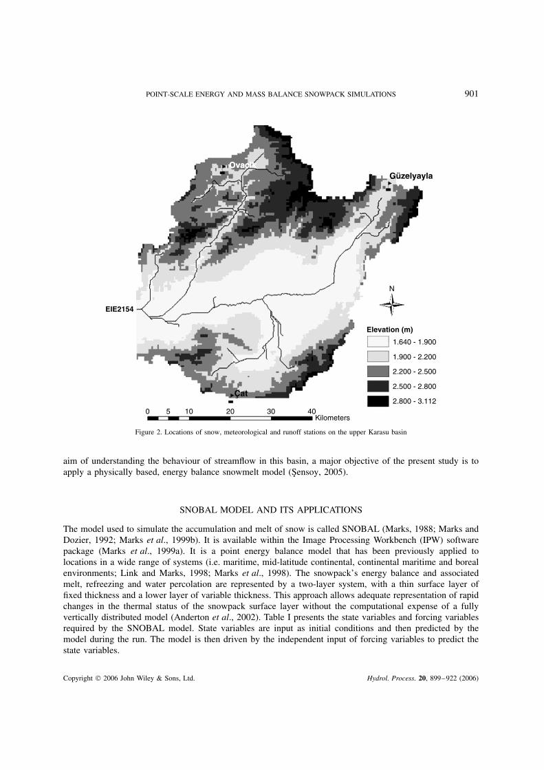
The Karasu basin, a sub-basin of the River Euphrates, is the test basin for this study (Figure 1). The regionis mountainous and, according to the long-term analysis of the hydrographs, snowmelt constitutes 60–70%of total annual streamflow volume (Kaya, 1999). Most of the water that originates from snowmelt contributesto large reservoirs located on the River Euphrates in Turkey. The study area is basically the headwaters,the upper Karasu basin, represented by the drainage area of stream gauging station 2154 (40°450E, 39°560N;Figure 2). The basin has an area of 2818 km2, and the elevation within the basin ranges from 1640 to 3112 m,with a hypsometric mean elevation of 2112 m. The area is predominately steppe (a plain without trees otherthan those near rivers), which may be semi-desert or covered with grass or shrubs or both, depending on theseason; forest cover is only 1Ð5% of the total basin area.

Although there have been previous applications of snowmelt models in this basin (e.g. Snowmelt RunoffModel (Kaya, 1999; Tekeli, 2005); HBV (Sorman, 2005); HEC-1 (Sensoy et al., 2003)), these are all based onthe degree-day approach and cannot be used to evaluate the energy dynamics of snowmelt. With the ultimate

ErzurumEIE2154

EIE2151

ErzincanEIE2119

44°30’

39°00’

33°30’

26°30’ 37°00’ 47°30’

26°30’ 37°00’ 47°30’

33°30’

39°00’

44°30’

stream-gaugesCities. dbfriverbasin

20 0 20 40 Kilometers

N

Figure 1. Location of Karasu basin in the upper Euphrates

Copyright 2006 John Wiley & Sons, Ltd. Hydrol. Process. 20, 899–922 (2006)

POINT-SCALE ENERGY AND MASS BALANCE SNOWPACK SIMULATIONS 901

EIE2154

Çat

OvacikOvacikGüzelyayla

1.640 - 1.900

1.900 - 2.200

2.200 - 2.500

2.500 - 2.800

2.800 - 3.112

Elevation (m)

0 5 10 20 30 40Kilometers

N

Figure 2. Locations of snow, meteorological and runoff stations on the upper Karasu basin

aim of understanding the behaviour of streamflow in this basin, a major objective of the present study is toapply a physically based, energy balance snowmelt model (Sensoy, 2005).

SNOBAL MODEL AND ITS APPLICATIONS

The model used to simulate the accumulation and melt of snow is called SNOBAL (Marks, 1988; Marks andDozier, 1992; Marks et al., 1999b). It is available within the Image Processing Workbench (IPW) softwarepackage (Marks et al., 1999a). It is a point energy balance model that has been previously applied tolocations in a wide range of systems (i.e. maritime, mid-latitude continental, continental maritime and borealenvironments; Link and Marks, 1998; Marks et al., 1998). The snowpack’s energy balance and associatedmelt, refreezing and water percolation are represented by a two-layer system, with a thin surface layer offixed thickness and a lower layer of variable thickness. This approach allows adequate representation of rapidchanges in the thermal status of the snowpack surface layer without the computational expense of a fullyvertically distributed model (Anderton et al., 2002). Table I presents the state variables and forcing variablesrequired by the SNOBAL model. State variables are input as initial conditions and then predicted by themodel during the run. The model is then driven by the independent input of forcing variables to predict thestate variables.



Table I. State variables predicted by the model and forcing variables required by themodel

State variables Forcing variables

Snow depth (m) Precipitation (mm)Snow density (kg m�3) Net solar radiation (W m�2)Snow surface layer temperature (°C) Incoming thermal radiation (W m�2)Average snow cover temperature (°C) Air temperature (°C)Average snow liquid water content (%) Vapour pressure (Pa)

Wind speed (m s�1)Soil temperature (°C)

The model was applied to three representative sites in the upper Karasu basin, namely Guzelyayla (GY),Ovacık (OVA) and Cat (CAT). GY station (2065 m) is located on the northeast edge of the basin, and thegeneral climatological conditions indicate that it is a cold, dry and windy site. OVA (2130 m), located onthe north-northwest edge of the basin, is a cold and dry site. CAT (2340 m) is the highest automatic weatherstation (AWS) in Turkey, and it is at the south boundary of the basin. Both GY and CAT have an unobstructedfetch in the prevailing wind direction of northeast to southwest.

There are a total of five model applications: GY applications during 2002–04 and OVA and CATapplications for the 2003–04 snow season. Therefore, there are three temporally distributed point modelapplications at one site (GY for 2002–04) and the areal evaluation of three point applications for one snowseason (GY, OVA, CAT for 2003–04 snow season). In all of these applications, a 2 h computational timestep was used.

INSTRUMENTATION

Although there is a considerable amount of snow in eastern Turkey, the existing data infrastructure indicatedthat it was necessary to collect additional data for model applications. The decision was made to instrument anew station (GY), which then was supplemented by upgrading of others (OVA, CAT) and, most importantly,for data to become transferable in real time. These station locations were chosen to cover the range ofcharacteristics (i.e. distributed over the basin at different elevations and climatic conditions) that can beobserved in this mountainous region of the world, where the canopy effect is negligible, considering inaddition the completeness and availability of meteorological data for model forcing.

Table II gives information on the AWSs along with their respective climate data measurements. The datacollection program consisted of continuous automated measurements of a number of hydrometeorologicalvariables at AWSs and manual snow surveys carried out with snow tubes monthly or bimonthly around theAWSs. Even the most common meteorological parameters are difficult to measure continuously at a remotesite, because recording equipment exhibits varying degrees of instability depending on the environmentalconditions.

The measurements of albedo, atmospheric/terrestrial longwave radiation and lysimeter yield are pioneerapplications in Turkey. The new measurements enable the development of a high-quality time series ofintegrated climate data and the evaluation of the components of the energy balance of the snow cover.

ENERGY AND MASS BALANCE CALCULATIONS

In a seasonal snow cover, metamorphic changes and melting are driven by temperature and vapour densitygradients within the snowpack, which are caused by heat exchange at the snow surface and at the snow–soil



Table II. Instrumentation at the sitesa

Snow data(sensor models)

Radiation(sensor models)

Climate data (sensor models) Datatransfer

Guzelyayla(GY)(2065 m)

SWE (Sensotec)Snow depth (Judd)Lysimeter

Net (0Ð3–100 µm) (Kipp &Zonen (NR Lite))

Solar, albedo (0Ð3–2Ð8 µm)

Precipitation (Met One)Temperature (Vaisala)Wind speed and direction (Met One)

Cable

(Kipp & Zonen (CM3)) Humidity, air pressure (Vaisala)

Ovacık(OVA)(2130 m)

SWE (Druck)Snow depth (Judd)

Solar, albedo (0Ð3–2Ð8 µm)(Kipp & Zonen (CM3))

Longwave (in/out; (5–25 µm)

Precipitation (Met One)Temperature (Vaisala)Wind speed (Young)

Cable

(Kipp & Zonen (CG2)) Humidity (Vaisala)

Cat(CAT)(2340 m)

SWE (Druck)Snow depth (Judd)

Net (0Ð3–100 µm) (Kipp &Zonen (NR Lite))

Solar (0Ð305–2Ð8 µm) (Kipp &

Temperature (Vaisala)Wind speed and direction (Met One)Humidity (Vaisala)

Inmarsat

Zonen (CM3)) Air pressure (Vaisala)

a Commercial names are listed for information purposes only and are neither an endorsement nor a critique by the authors.

interface. In general, the energy balance of a snow cover is expressed as

Q D Rn C H C LvE C G C M �1�

where Q �W m�2� is change in snow cover energy, and Rn, H, LvE, G and M (all W m�2) are net radiative,sensible, latent (Lv is the latent heat of vaporization and E is the mass of water evaporated or condensed),ground (conductive) and advective energy fluxes respectively.

SNOBAL simulates each component of the snow cover energy balance and accumulates mass and thermalconditions for the next time step. It predicts melt in two snow cover layers and runoff from the base of thesnow cover, and it adjusts the snow cover mass, thickness and thermal properties at each time step. If thecomputed energy balance is negative, then the cold content increases, and the layer temperature decreases.If the energy balance is positive, then the layer cold content decreases until it is zero. Additional input ofenergy causes the model to predict melt. If melt occurs, then it is assumed to displace air in the snow cover,causing densification and increasing the average liquid water content of both layers. Liquid water in excessof a specified threshold becomes meltwater outflow.

MODEL INPUTS

Surface roughness

The effective snow surface roughness, required for the turbulent transfer calculations, has been shown tobe a dynamic property that is dependent on wind speeds and microtopography of the snow surface (Andreas,1987). It is difficult to measure and, therefore, is usually estimated based on values reported in the literatureranging from 0Ð0001 to 0Ð01 m (Anderson, 1976; Moore, 1983), depending on snow depths and conditions.It is a site-specific and dynamic value, and it is not possible to determine an exact value for these sites.Testing was done during the initial model application phase using the physically realistic values referred toin the literature. The trial that gave the best fit with the observations was assumed to be the correct value forroughness. Roughness length was set to 0Ð001 m for GY and CAT, but it was 0Ð0001 for OVA, where thewind speeds are low, since it has been found that the aerodynamic roughness increases with increasing windspeed due to the influence of the drifting snow (Marsh, 1999). Unfortunately, there is no previous researchon sublimation of blowing snow at the site, and SNOBAL does not include an explicit parameterization for



blowing snow; therefore, the decision on surface roughness length depends directly on the average wind speedvalues at the sites. Surface roughness affects turbulent fluxes, and turbulent fluxes usually comprise a smallcomponent of the overall snow cover energy balance; therefore, the seasonal simulation should be relativelyinsensitive to roughness length.

Precipitation data

The rates and volumes of snowfall are very difficult to evaluate from precipitation gauge records (withoutheater) because they are affected not only by wind, site characteristics and precipitation intensity but alsoby variations in the density and structure of the snow crystals as they fall. Since the sites are cold (andwindy for GY and CAT), there is an undercatch and freezing problem for snowfall; the recorded valuesare unrealistically small compared with snow depth and SWE at the stations and snowfall values of otherstations. This underestimation is improved by the information gathered from the snow data measured withsnow pillows and also from the nearby microclimatologic stations.

One common way of dealing with this is to use the change in SWE values for precipitation computation(e.g. method for editing precipitation data used by Garen and Marks (2001)). Such an analysis was carriedout with the data provided from the GY site and the surrounding meteorological stations. The data acquiredfrom another station that shows similar patterns with GY in terms of snow depth, SWE and air temperaturesprovided verification for the precipitation analysis at GY. First, daily precipitation amounts were computedaccording to changes in SWE (with some appropriate data quality checks and editing), then a simple fractioningapproach was used to disaggregate the daily fields into 2 h fields. Precipitation values were corrected andcomputed for OVA and CAT with the same methodology.

Net shortwave radiation

Net shortwave radiation is the incoming radiation minus that reflected from the snow surface. The snowalbedo, therefore, is a key parameter affecting the net shortwave radiation, as it defines how much of theincoming solar radiation is reflected from the surface. The snow albedo shows seasonal and daily variationsdepending on a wide variety of factors, like solar zenith angle, aging, wetness, impurity content, particlesize, snow density and composition, surface roughness, cloud cover and spectral composition. Albedo iscontinuously observed at GY, except for the first winter (2002), with a set of pyranometers that are used tomeasure solar radiation and reflection in the range 0Ð305–2Ð8 µm.

It was decided to replace the physically based algorithm of albedo computation (dependent on snow grainsize and sun angle) usually used with the SNOBAL model (i.e. the module ALBEDO in the IPW softwarepackage; Marks et al., 1999a) with a new parameterized scheme developed specifically for the site using theobserved data for the 2002–03 snow season, since there is a lack of measured data either for albedo or grainsize. This scheme is based on a scenario using both a linear parameterization (Equation (2)) derived fromprincipal component analysis (PCA) and an albedo decay function determined from aging (Equation (3)). PCAwas applied to the observed data at GY for the 2002–03 snow season, which led to the selection of snowdepth, global radiation and temperature as predictor variables, then stepwise regression was used to derivecoefficients for normalized variables. The second equation is simply based on snow aging. The two equationswere applied depending on the occurrence (Equation (2)) or non-occurrence (Equation (3)) of snowfall. Themodel results are shown in Figure 3; observed and modelled albedo values are presented both in 2 h and indaily time steps, besides the linear relationship and best fit with the daily data for the melting period of 2003at GY. The same modelling approach was also used for CAT, where there is no albedo measurement duringthe model application of the 2003–04 snow season.

Albedo D 0Ð75 C 0Ð185d � 0Ð1Si � 0Ð0001Tair �2�

Albedo D 0Ð77 � 0Ð15 ln�t� �3�



0.2

0.4

0.6

0.8

1

Tw

o H

ourl

y A

lbed

o

Observed Albedo Modeled Albedo

0.2

0.4

0.6

0.8

1.0

01-M

ar-0

3

05-M

ar-0

3

09-M

ar-0

3

13-M

ar-0

3

17-M

ar-0

3

21-M

ar-0

3

25-M

ar-0

3

29-M

ar-0

3

02-A

pr-0

3

06-A

pr-0

3

10-A

pr-0

3

14-A

pr-0

3

Dai

ly A

lbed

o

y = 1.0107xR2 = 0.8818

0.0

0.2

0.4

0.6

0.8

1.0

0.0 0.2 0.4 0.6 0.8 1.0

Observed Albedo

Mod

eled

Alb

edo

Figure 3. Observed and modelled albedo values for 2003 snowmelt period, GY

where d is snow depth, Si is the global radiation and Tair is the air temperature, all of which are normalizedand, therefore, are unitless; t (days) is aging time from the last snowfall. The albedo values thus estimatedwere used to determine the reflected shortwave radiation, which was subtracted from the measured incomingradiation to obtain net shortwave radiation.

Incoming longwave radiation

There is no measured incoming thermal radiation at GY and CAT stations; therefore, the snow surfacetemperature was computed as a residual. Snow surface temperature is difficult to measure by physicalthermometry, but Davis et al. (1984) showed that the near-surface temperature of the snow tends to follow theair temperature. This occurs because the insulating characteristics of the snow cover allow the surface layerto come into temperature equilibrium with the atmosphere even though this may create large temperaturedifferences between the surface and lower layers.



Since the snow surface temperature values were measured manually for a brief period of time at GYand OVA stations, a linear relation between air and snow surface temperatures was developed using 43observations, with r2 D 0Ð89:

Tsnow D 1Ð02Tair � 3Ð17 �4�

where Tsnow (°C) is the snow surface temperature and Tair (°C) is the air temperature, with the constraint ofmaximum Tsnow D 0 °C. Incoming longwave radiation is calculated using measured net radiation values as

Li D Rnet � Snet C εsnow�T4snow �5�

where Li �W m�2� is the incoming longwave radiation, Rnet �W m�2� is the net radiation, Snet �W m�2� isthe net shortwave radiation, εsnow is the emissivity of the snow surface (0Ð99), Tsnow (K) is the snow surfacetemperature and � is the Stefan–Boltzmann constant (5Ð67 ð 10�8 W m�2 K�4).

Net longwave observations at OVA were used to check the snow surface temperature computations. Snowsurface temperature values were computed from measured terrestrial longwave radiation (Tsnow�observed) andthen compared with the results of the empirical formula (Tsnow�modelled) (Equation (4)). Figure 4 presents therelation between air temperature Tair and snow surface temperature in terms of both the observed valueswith the pyrgeometer (Tsnow�observed) and computed ones derived from the empirical formulation of manualmeasurements (Tsnow�modelled). Although there is considerable scatter in the relation between the two data sets,a strong correlation is found between them. According to these graphics, the empirical equation adequatelyrepresents the snow surface temperature values overall (the first graphic in Figure 4); however, it may bemore appropriate to separate the equation into two parts, one for the afternoon hours (12 : 00–16 : 00) atwhich the air temperatures will be relatively high (the last graphic in Figure 4) and one for the rest of theday (the second graphic in Figure 4), for which the equation explains about 90% of the relation. The maindiscrepancies occur when the air temperature is above freezing, since the snow surface should be at freezingwhen the air temperature is higher (Shusun et al., 1999).

Although several longwave radiation models have been developed (e.g. Satterlund, 1979; Idso, 1981),and these models can successfully represent daily average atmospheric longwave radiation with cloud covercorrection, they are not adequate to represent diurnal variations for a 2 h computational time step. Therefore,it was preferred to use snow surface temperature data together with observed radiation values to computeincoming longwave radiation as a residual (Equation (5)) instead of other empirical models.

Air temperature, vapour pressure and wind speed

Vapour pressure for the individual sites was computed from site air temperatures and relative humidityvalues using standard meteorological algorithms. In contrast to GY and CAT, where average wind speeds arearound 3Ð5 m s�1 and 4 m s�1 respectively during the snow season, wind speeds are lower at OVA, with anaverage of 1Ð5 m s�1. OVA is also distinct in that its temperatures are cooler than one would expect basedon its elevation and the temperature trends based on the other sites.

Soil temperature

Since the sites appear to be cold and sometimes have a shallow snowpack, setting the soil temperatureto a constant of 0 °C is not a feasible assumption, since this led to an unrealistically high simulated heattransfer from the soil to the snow. Therefore, the soil temperature data from another station with similar snowaccumulation and melt patterns were used for soil temperatures at 20 cm depth.

Although the model was applied in 2 h time intervals, the climate input data are presented in 5-day averagesfor clearer illustration in Figure 5. The model applications have shown that the initiation of snowmelt andthe melt rate are very sensitive to relatively minor changes in climate forcing. To simulate the snow coverprocesses correctly, it is essential to use forcing data that account for these minor variations.



y = 0.9817x - 5.0345R2 = 0.8129

-40-35-30-25-20-15-10

-505

10

-30 -25 -20 -15 -10 -5 0 5 10 15T

snow

(°C

)

Pyrgeometer Empiric Linear (Pyrgeometer)

(Except hours 1200, 1400, 1600)

y = 1.0987x - 3.0669R2 = 0.9144

-40

-35

-30

-25

-20

-15

-10

-5

0

5

10

-30 -25 -20 -15 -10 -5 0 5 10 15

(Hours 1200, 1400, 1600)

y = 1.0774x - 7.1178R2 = 0.6003

-40-35-30-25-20-15-10

-505

10

-30 -25 -20 -15 -10 -5 0 5 10 15

Tair (°C)

Tsn

ow (

°C)

Tsn

ow (

°C)

Figure 4. Snow surface (Tsnow�observed by pyrgeometer, Tsnow�modeled by empirical formula) and air temperature Tair relations, OVA, 2004

MODEL OUTPUTS

The results are analysed under two main topics with two more subtopics under each. The first topic is thetemporal analysis of the point applications at one station for three consecutive snow seasons, and the secondis the areal analysis of the point applications at three stations for one snow season. Each analysis is furtherevaluated both in terms of snow cover energy balance and in terms of snow cover mass balance.

Temporal analysis of point applications

Compared with the long-term averages, including manual snow course measurements at GY, OVA and CATbetween the years 1976 and 2003, the first two snow seasons were average years, whereas SWE values werewell above average during the peak period of 2004. Although there are similarities between snow seasons interms of snowfall, melt patterns have different characteristics for each year. The removal of snowpack from



200

100

0

300

200

100

010

0

-10

-20

600

400

200

0

6

4

2

0

2001 - 2002 2002 - 2003 2003 - 2004

6-10

Dec

16-2

0 D

ec

26-3

1 D

ec

6-10

Jan

16-2

0 Ja

n

26-3

1 Ja

n

6-10

Feb

16-2

0 F

eb

26-2

9 F

eb

6-10

Mar

16-2

0 M

ar

26-3

1 M

ar

6-10

Apr

Net Shortwave (W/m2)

Incoming Longwave (W/m2)

Temperature (°C)

Vapor Pressure (Pa)

Wind Speed (m/s)

Figure 5. Model input parameters at GY during 2002–04 snow seasons

GY occurred within the interval of 10–15 April for all 3 years. However, the snow covered area images fromsatellites (NOAA and MODIS) indicated gradual melting for the year 2004, especially at the high elevationzones, in contrast to the sharp melting period observed for the year 2003.

Snow cover energy balance. Figure 6 depicts energy flux outputs in 5-day averages for each season, includingnet radiation, turbulent energy (includes both sensible and latent heat fluxes), ground heat flux and total energy;advective energy is not shown because it is very small in amount. Below, simulations for each of the 3 yearsat GY are analysed in detail.

2001–02, GY: Snowmelt runoff started in the 1–5 March 2002 time period with an increased net radiationeffect. Gradual melting developed continuously until 15 April, with net radiation and turbulent heat fluxesdominating. The greatest negative net turbulent heat fluxes occurred within the period of 6–10 March. The



100

50

0

-50

100

50

0

-50

100

50

0

-50

100

50

0

-50

6-10

Dec

16-2

0 D

ec

26-3

1 D

ec

6-10

Jan

16-2

0 Ja

n

26-3

1 Ja

n

6-10

Feb

16-2

0 F

eb

26-2

9 F

eb

6-10

Mar

16-2

0 M

ar

26-3

1 M

ar

6-10

Apr

Net Radiation (W/m2)

Turbulent Heat (W/m2)

Ground Heat (W/m2)

Total Energy (W/m2)

2001 - 2002 2002 - 2003 2003 - 2004

Figure 6. Model outputs for energy flux terms at GY during 2002–04 snow seasons

basic reason is the climate conditions on 9 March, on which 8Ð25 m s�1 wind speed was observed, althoughthe average wind speed for the 5-day period was 2Ð62 m s�1 (Figure 5). On this day, the vapour pressurewas very low, around 200 Pa, and the average temperature decreased by 5 °C. Under these conditions, boththe sensible and latent heat fluxes were generally negative, since the air was both colder and less humidthan the snow surface, and the high wind speed enhanced this negative turbulent heat flux. During the period11–15 March, air temperatures turned to positive values, and there was significant cloud cover, resulting inthe highest incoming longwave radiation for the season (Figure 5). A sudden increase in wind speeds during21–25 March coincided with a reaccumulation of snow and also directly affected sensible heat flux, since theair temperatures were around 0 °C. Both the sensible and latent heat fluxes were generally positive during thisperiod; together, these explain more than 50% of the total energy for snowmelt during this interval (Figure 7).Precipitation falling as snowfall during 6–10 April caused a sharp latent heat flux increase, which explainshalf of the total energy. Finally, for the last interval, Q yielded an amount of melt due to high net radiation,which was around 80% of the total energy.



-100%

-50%

0%

50%

100%

GY

, 200

1-20

02G

Y, 2

002-

2003

GY

, 200

3-20

04

Rnet H+L G M

01-0

5 D

ec11

-15

Dec

21-2

5 D

ec1-

5 Ja

n11

-15

Jan

21-2

5 Ja

n1-

5 F

eb11

-15

Feb

21-2

5 F

eb1-

5 M

ar11

-15

Mar

21-2

5 M

ar1-

5 A

pr11

-15

Apr

21-2

5 A

pr

-100%

-50%

0%

50%

100%

-100%

-50%

0%

50%

100%

Figure 7. Energy percentages within the total energy at GY

2002–03, GY: Sensible heat fluxes oscillated in direction during the snow season, whereas latent heat fluxestended to be negative through the season, indicating evaporative cooling of the snow cover. Since the siteis dry and cold, observed sensible and latent heat fluxes were small in amount, although the wind speedswere rather high, averaging a little over 3 m s�1. In contrast to the 2001–02 snow season, accumulation wascontinuous until the beginning of April 2003, and then a sharp ablation period started on 3 April, endingon 15 April. Increases in average air temperature and wind speed, from �12Ð7 to �0Ð2 °C and from 2Ð7 to3Ð9 m s�1 respectively (26–31 March to 1–5 April), led to a drastic increase in sensible heat flux, whichinitiated the snowmelt. From then on, net radiation constituted around 70% of the overall energy (Figure 7).

2003–04, GY: The accumulation period continued until an unusual flood event occurred during 29February–6 March 2004 due to increased turbulent flux and rain on snow (ROS). The precipitation in the form



of rainfall, due to positive air temperatures, contributed to positive advective energy and, more importantly,caused an increase in the specific mass of the existing snow cover. Turbulent heat flux increased to 76Ð3% ofthe total energy (Figure 7), which is the maximum value of all 3 years. Similarly, advective energy increasedto 2Ð17 W m�2 at the end of February. Higher temperatures and vapour pressures increased the net turbulentheat, which led to melting of the already isothermal snow. As the event ended and conditions cleared, therewas a sharp drop in incoming longwave radiation. After the cold and cloudy period, the snowmelt restartedon 22 March at a much more moderate rate with the net radiation dominating. During the next 5 days,temperatures decreased, accompanied by high winds, resulting in rather low turbulent heat. Finally, with thenet radiation increase, snow cover disappeared on 11 April.

In summary, the year 2002 was different from the other 2 years, with an early melt as a result of solarradiation and an extensive melt period of approximately 1Ð5 months. The year 2003 was distinguished by asharp and short melt period, starting with high turbulent heat and continuing with high net radiation, endingalmost within 10 days. The year 2004 was characterized by a flood due to high turbulent heat fluxes and anROS event. The timing of snowmelt is comparable for the last 2 years except for the ROS event.

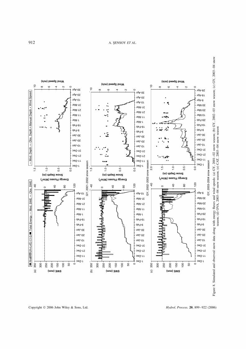
Snow cover mass balance. Simulated snow cover mass is compared with measured mass in terms of bothSWE and snow depths (Figure 8a–c) for model verification in 2 h time steps. The model converts rain directlyto runoff when no snow cover is present. When snow is present, runoff is the sum of melt, less the liquidwater holding capacity of the snow, plus rainfall. Early in the spring, the model simulated several minor meltevents that do not exceed the water holding capacity of the snowpack at the site. Model simulation resultsare in close agreement with the continuous snow pillow data throughout the snow season, except for somediscrepancies due to accuracy issues with the snow pillow observations, as described below.

The continuous automatic depth measurements are used to validate the simulated snow depths (Figure 8a–c).Although the total change in snow depth is modelled well over the whole snow season, there are periods whenthe model seems both to over- and underestimate the snow depths. In addition, mean depth measurementsrecorded manually during bimonthly snow course surveys provided an additional validation data set. Windspeed values greater than 6Ð5 m s�1 are also plotted to show its effect on redistribution of snowfall during theaccumulation phase. The deviations between the model results and the measured snow depth (also SWE) areobserved during the pronounced windy periods, since the model does not include an explicit parameterizationfor blowing snow.

Snow lysimeters are used to provide a physical measurement for testing models of snowpack energybalance and/or meltwater production (Kattelman, 2000). Therefore, the simulated snowmelt runoff values arealso compared with measured yield/discharge from the lysimeter for the years 2003 and 2004 at GY. Figure 9shows time series of observed and modelled meltwater outflow from the base of the snowpack for the year2003.

Two snowmelt test periods, 5–10 April 2003 (SM-I) and 11–14 April 2003 (SM-II), are examined below.During SM-I, a significant reduction in SWE occurred with an increase in lysimeter discharge. There is atime lag of approximately 1 day for the lysimeter to start yielding; although it is possible that there are errorsin how SNOBAL handles the delay of meltwater as it flows through the snowpack, known problems withthe lysimeter (such as freezing) make this the more likely error source. Nevertheless, the lysimeter melt ratesare comparable to the modelled rates (Figure 9b). Following a cold period with little melt on 4 April, dailypeak outflow magnitudes rapidly increased to over 3 mm h�1, with very sharply peaked daily hydrographs.The timing of modelled outflow is generally excellent for both the peaks and troughs for the following days.There is a discrepancy, however, in the magnitudes of modelled and observed values. During SM-II, thelysimeter did not indicate any corresponding significant yield increase. A number of reasons can be stated forthe different lysimeter responses between SM-I and SM-II. One reason may be a tipping-bucket failure dueto extensive melting and rainfall followed by a period of rainfall on 8–10 April. Other reasons could be:



0.0

0.5

1.0

1.5

0246810

1-Dec

11-Dec

21-Dec

31-Dec

10-Jan

20-Jan

30-Jan

9-Feb

19-Feb

1-Mar

11-Mar

21-Mar

31-Mar

10-Apr

20-Apr

30-Apr

Snow Depth (m)

Wind Speed (m/s)

0.0

0.5

1.0

1.5

1-Dec

11-Dec

21-Dec

31-Dec

10-Jan

20-Jan

30-Jan

9-Feb

19-Feb

1-Mar

11-Mar

21-Mar

31-Mar

10-Apr

20-Apr

30-Apr

Snow Depth (m)

0246810

Wind Speed (m/s)

Mod

. Dep

thO

bs. D

epth

Man

ual D

epth

Win

d S

peed

c

050100

150

200

250

300

350

1-Dec

11-Dec

21-Dec

31-Dec

10-Jan

20-Jan

30-Jan

9-Feb

19-Feb

1-Mar

11-Mar

21-Mar

31-Mar

10-Apr

SWE (mm)

-40

0 40 80 120

Energy Fluxes (W/m2)

Rne

t(H

+Lv

E)

GT

otal

Ene

rgy

Mod

. SW

EO

bs. S

WE

(a)

1-Dec

11-Dec

21-Dec

31-Dec

10-Jan

20-Jan

30-Jan

9-Feb

19-Feb

1-Mar

11-Mar

21-Mar

31-Mar

10-Apr

050100

150

200

250

300

350

SWE (mm)

-40

40 80 120


(b)

0

GY

, 200

3-20

04 s

now

sea

son

GY

, 200

2-2

003

snow

sea

son

GY

, 200

1-20

02 s

now

sea

son

050100

150

200

250

300

350

1-Dec

11-Dec

21-Dec

31-Dec

10-Jan

20-Jan

30-Jan

9-Feb

19-Feb

29-Feb

10-Mar

20-Mar

30-Mar

9-Apr

SWE (mm)

-40

0 40 80 120


0.0

0.5

1.0

1.5

2.0

1-Dec

11-Dec

21-Dec

31-Dec

10-Jan

20-Jan

30-Jan

9-Feb

19-Feb

29-Feb

10-Mar

20-Mar

30-Mar

9-Apr

19-Apr

29-Apr

Snow Depth (m)

0246810

Wind Speed (m/s)

(c)

Figu

re8.

Sim

ulat

edan

dob

serv

edsn

owda

taal

ong

with

ener

gyflu

xes

and

win

dsp

eeds

:(a

)G

Y,

2001

–02

snow

seas

on;

(b)

GY

,20

02–

03sn

owse

ason

;(c

)G

Y,

2003

–04

snow

seas

on;

(d)

OV

A,

2003

–04

snow

seas

on;

(e)

CA

T,

2003

–04

snow

seas

on



0.0

0.5

1.0

1.5

2.0

2.5

Snow Depth (m)

0246810

Wind Speed (m/s)

0

100

200

300

400

500

1-Dec

11-Dec

21-Dec

31-Dec

10-Jan

20-Jan

30-Jan

9-Feb

19-Feb

29-Feb

10-Mar

20-Mar

30-Mar

9-Apr

19-Apr

29-Apr

1-Dec

11-Dec

21-Dec

31-Dec

10-Jan

20-Jan

30-Jan

9-Feb

19-Feb

29-Feb

10-Mar

20-Mar

30-Mar

9-Apr

19-Apr

29-Apr

SWE (mm)

-40

0 40 80 120

160

200


(d)

Mod

. Dep

thO

bs. D

epth

Man

ual D

epth

Win

d S

peed

Rne

t(H

+Lv

E)

GT

otal

Ene

rgy

Mod

. SW

EO

bs. S

WE

0.0

0.5

1.0

1.5

2.0

2.5

1-Dec

11-Dec

21-Dec

31-Dec

10-Jan

20-Jan

30-Jan

9-Feb

19-Feb

29-Feb

10-Mar

20-Mar

30-Mar

9-Apr

19-Apr

29-Apr

Snow Depth (m)0246810

Wind Speed (m/s)

0

100

200

300

400

500

1-Dec

11-Dec

21-Dec

31-Dec

10-Jan

20-Jan

30-Jan

9-Feb

19-Feb

29-Feb

10-Mar

20-Mar

30-Mar

9-Apr

19-Apr

29-Apr

SWE (mm)

-40

0 40 80 120

160

200


(e)

CA

T, 2

003-

2004

sno

w s

easo

n

OV

A, 2

003-

2004

sno

w s

easo

n

Figu

re8.

(Con

tinu

ed)



0

100

200

300

1-A

pr-0

3

2-A

pr-0

3

3-A

pr-0

3

4-A

pr-0

3

5-A

pr-0

3

6-A

pr-0

3

7-A

pr-0

3

8-A

pr-0

3

9-A

pr-0

3

10-A

pr-0

3

11-A

pr-0

3

12-A

pr-0

3

13-A

pr-0

3

14-A

pr-0

3

15-A

pr-0

3

Ru

no

ff, L

ysim

eter

Y

ield

, SW

E (

mm

)

Obs. SWE Runoff Lysimeter Yield

(a)

0

2

4

6

8

10

12

1-A

pr-0

3

2-A

pr-0

3

3-A

pr-0

3

4-A

pr-0

3

5-A

pr-0

3

6-A

pr-0

3

7-A

pr-0

3

8-A

pr-0

3

9-A

pr-0

3

10-A

pr-0

3

11-A

pr-0

3

12-A

pr-0

3

13-A

pr-0

3

14-A

pr-0

3

15-A

pr-0

3

Ru

no

ff, L

ysim

eter

Y

ield

(m

m /

2hr)

Runoff Lysimeter Yield

(b)

Figure 9. (a) SWE, cumulative modelled runoff and lysimeter yield, GY, 2003. (b) Two-hourly rates of modelled runoff and lysimeter yield,GY, 2003

1. The non-uniformity of snow depth distribution within the snow station; thus, the lysimeter might have asnow depth that is less than that on the snow pillow.

2. The difference between the areas of the lysimeter (1Ð53 m2) and snow pillow (6Ð50 m2) may be anotherreason for the different lysimeter responses between SM-I and SM-II.

3. The difference in the material between the lysimeter (galvanized steel) and the snow pillow (hypalon) mighthave resulted in an increased evaporation rate from the lysimeter (Tekeli et al., 2005).

A plot of observed and modelled cumulative basal meltwater outflow (Figure 9a) clearly illustrates thedifferences. Since similar problems were encountered, results are not presented for the year 2004.

Areal evaluation of point applications

From the SWE graphs (2003–04), it can be seen that the whole snow season can be broken into segmentsbased on climatic conditions (Figure 8c–e). The snow cover development occurred during the period from1 December 2003 to 29 February 2004. A series of cold storms deposited significant amounts of snow on10–11 February and 21–22 February; 16–25 February was one of the coldest periods through the wholesnow season, with temperatures well below freezing (�10 to �20 °C) and high wind speeds observed at allthe stations; 22–29 February was a very cold, fairly clear period. See Figure 10 for input data categorization.

The 29 February–6 March event was accompanied by high winds and intense rainfall, which was one ofthe most intense ROS events ever recorded. The station at the Erzurum airport reported rainfall of about



0

200

400

600

0

2

4

6

8

-15

-10

-5

0

5

10

0

100

200

300

0

100

200

300

400

Net Shortwave(W/m2)

Incoming Longwave (W/m2)

Temperature (°C)

Vapor Pressure(Pa)

Wind Speed (m/s)

1 Dec−29 Feb 29 Feb−6 Mar 6−20 Mar 20−31 Mar 1−6 Apr 6−30 Apr

GY OVA CAT

Figure 10. Model input parameter categorization at GY, OVA, CAT, 2003–04 season evaluation

50 mm during the event. Intense rainfall combined with rapid snowmelt contributed to the flood event. Peakflows on headwater streams and rivers draining the upper Karasu basin (station 2154) occurred on 6 March2004, when the river rose from 10 m3 s�1 on 29 February to 120 m3 s�1 by 6 March.

Low air temperature, vapour pressure and solar radiation clearly indicate the period for the developmentof snow cover (1 December–29 February). In contrast, climate conditions during the ROS event show areduction in solar radiation, air temperature always above freezing and an increase in vapour pressure to nearor above the saturated vapour pressure at 0 °C. During the ROS event, air temperatures were above freezing,and there was a large humidity gradient towards the snow cover at all three sites (which can be observedfrom hourly data).

Snow cover energy balance. A few minor deposition events occurred during the last week in October andthe last week in November, but these melted rapidly and did not persist for more than 2 or 3 days. Duringthe snowpack development phase, the net turbulent flux fluctuated between 0 and 10 W m�2 at GY and CAT



(Figure 11). In contrast, it was around zero at OVA, where LvE and H displayed the common characteristicduring non-storm periods that they were of the same magnitude but opposite in sign. Thus, total energyremained around zero, with the dominating negative effect of net all-wave radiation during this snowpackdevelopment phase (1 December–29 February; Figure 11).

During the ROS event (29 February–6 March), the snow cover energy balance was quite different, asall sites had a distinctly positive energy balance with a large input of turbulent energy (Figure 11). Boththe sensible and latent heat fluxes were positive and combined to enhance the snow cover energy balancesignificantly. Turbulent fluxes constituted around 85% of total energy at GY and CAT for the period of1–5 March, but this value was 30% for OVA (Figure 12). The advective energy became effective andsignificant for the first time in terms of percent of total energy (Figure 12). The result was that totalenergy was large and positive throughout the ROS event, providing a substantial amount of energy forsnowmelt. Because of the influence of large volumes of 0 °C meltwater percolating into the soil column, thetemperature gradient between the soil and the snow was removed, and ground heat flux was unimportant(Figure 11).

-10

0

10

20

-0.4

-0.2

0

0.2

0.4

-250

255075

100125150

Ground Heat Flux (W/m2)

Advective Heat Flux (W/m2)

Total Energy (W/m2)

-250

255075

100125

GY OVA CAT

-30

-15

0

15

30

Rnet (W/m2)

Turbulent Heat Flux (W/m2)

1 Dec−29 Feb 29 Feb−6 Mar 6−20 Mar 20−31 Mar 1−6 Apr 6−30 Apr

Figure 11. Model output categorization at GY, OVA, CAT, 2003–04 snow season



-100%

-50%

0%

50%

100%

GY

, 200

3-20

04

Rnet H+L G M

-100%

-50%

0%

50%

100%

OV

A, 2

003-

2004

-100%

-50%

0%

50%

100%

01-0

5 D

ec11

-15

Dec

21-2

5 D

ec1-

5 Ja

n11

-15

Jan

21-2

5 Ja

n1-

5 F

eb11

-15

Feb

21-2

5 F

eb1-

5 M

ar11

-15

Mar

21-2

5 M

ar1-

5 A

pr11

-15

Apr

21-2

5 A

pr

CA

T, 2

003-

2004

Figure 12. Energy percentages within the total energy (GY, OVA, CAT)

The total energy balance was again around zero during the period immediately following the ROS event,6–20 March (Figure 11). Although the net solar energy had an increasing trend with the progression of theseason, net longwave radiation values were high but negative due to low temperatures and vapour pressures;all of these caused net all-wave radiation to be zero. In addition, extreme cold conditions caused both thesensitive and latent heat fluxes generally to be negative, which led to large negative turbulent fluxes.

During the clear sky period of 20–31 March, the increased net solar radiation under clear skies dominatedthe energy balance and constituted around 80 to 95% of the total energy at the three sites; total energyduring this period was effectively well above zero (Figure 12). The air temperatures were well above 0 °C,and positive turbulent heat fluxes were observed at GY and CAT, though negative turbulent heat occurred at



OVA, most probably due to negative air temperatures. Cloudy skies with rather low temperatures and vapourpressures caused both the latent and sensible heat fluxes to be negative and constitute 50% of total energyfluxes (Figure 12) during the mixed ROS event on 1–6 April. The last part (7 April and onward) is purely asnow-melting period with the considerable effect of net solar radiation (Figure 11). Snowpack disappeared inmid-April at GY, whereas it extended until the end of April at OVA and CAT (Figure 8c–e).

Snow cover mass balance. Simulated SWE matched observed SWE (Figure 8c–e) very closely during thedevelopment of the snow cover, especially at GY and OVA, whereas there is a deviation for CAT, whichis probably attributable to problems related to the snow pillow itself (see next section). In the same manneras the GY model application for 2003–04, there is a mismatch for the modelled and observed SWE valuesafter the ROS period. The two gaps in the observed record of OVA might be due to problems related withimproper functioning of the datalogger as a result of low temperatures.

The model has a tendency occasionally to estimate maximum snow depths exceeding the observations. Thisdifference is not consistent between stations and is difficult to explain. Although it is possible that the modelis in error due to inaccuracies in depicting snow density, it is more likely that the discrepancies are due toobservation errors. For example, there are unrealistically high accumulation records (Figure 8d), especiallyat OVA. It is possible that the ultrasonic depth gauge (UDG) record is in error, and the observed inaccurateaccumulation is due to refreezing of surface meltwater (which reduced the distance into the snowpack thatcould be detected) or the UDG is detecting the top of falling snow rather than the snowpack surface itself.

Melt with associated runoff production started during the first days of March and continued over a perioddifferent for each of the sites. The maximum sustained melt rate exceeded 6 mm h�1 at CAT, whereas itapproached 5 mm h�1 for OVA and was 5Ð5 mm h�1 at GY. Melt rates at CAT were comparable to those atGY; however, a substantially larger snowpack at CAT resulted in an extended ablation period, with completeablation occurring almost 2 weeks later than at GY.

SNOW PILLOW ERRORS

In general, snow pillows function adequately; however, long-term experience with snow pillows demonstratesthat they can yield unpredictable and erroneous results that make it difficult for water resource managers andresearchers to determine what is occurring (Johnson and Marks, 2004). There are error sources related to thesnow pillow, such as a leaking pillow or the occurrence of ice bridging and a connection with the snowpackoutside of the snow pillow causing a reduction of the measured pressure and calculated SWE. In addition,soil expansion is a real problem at the beginning of the snow season if rainfall occurred after the calibrationof a snow pillow.

SWE sensor errors are most severe during the transition from a cold to a warm snow cover when the0 °C isotherm progresses from the snow surface toward the ground. When the isotherm reaches the groundbefore reaching the sensor, heat from the ground can no longer be conducted into the snow, producing asudden increase in the snowmelt rate. This can cause an SWE sensor overmeasurement error that continuesto increase until the 0 °C isotherm reaches the top of the sensor (e.g. a sudden jump at OVA in Figure 8d).

Either under- or overmeasurement errors may occur at critical times when the snow cover transitions fromwinter to spring conditions and at the start of periods of rapid snowmelt. There was an unusual circumstancein early March 2004 in which precipitation fell as rainfall due to increased temperatures. Average dailytemperatures increased from �13Ð4 to C3Ð4 °C. Over the next several days, average temperatures becamevery cold, down to �10 °C. Because the snow pillow alters the thermal and moisture exchange between thesoil and snow, and because the soil was quite moist, it can be assumed that a significant transfer of vapourfrom the soil to the cold snowpack would have taken place prior to this ROS event. This vapour transfercould not have occurred over the snow pillow, so it can also be assumed that the snow over the snow pillowwould be colder and may have contained basal ice. Rainwater was probably retained above the snow pillow



until the thermal gradient was removed and the ice layers melted. At that time, a sudden reduction in SWEoccurred, much like the breaking of an ice dam, which would explain the rapid large loss of SWE reported atthe three stations (Figure 8c–e). Later manual snow samples indicated several very dense layers deep withinthe snowpack, as well as distributed ice lenses.

There is a similar pattern in the 2002–03 snow season simulation (Figure 8b): an amount of pre-meltingwithin the time period of 11–20 March 2003 due to net radiation resulted in ice bridging. The pack was notisothermal at this time, and sustained melt did not occur, which caused the sidewalls to carry the ice load,thus decreasing the pressure on the snow pillow during 26 March–1 April 2003.

VALIDATION STATISTICS

Validation measurements included snow depth measured with an ultrasonic depth sensor, SWE from snowpillows, manual observations of SWE and snow depth, and meltwater outflow from lysimeters. Modelperformance itself can be judged by visual comparison of time series of observed values and modelledoutput (e.g. SWE, snow depth, runoff) and with quantitative measures of goodness of fit. Three standardquantitative tests are used to evaluate model performance and the goodness of fit for the model applications.

The root-mean-squared error (RMSE) between simulated and observed values and the mean bias difference(MBD), or mean deviation of simulated from observed values, are presented below. The Nash–Sutcliffecoefficient or ‘model efficiency’ (ME), which describes the variation in the observed parameter accountedfor by the simulated values (Nash and Sutcliffe, 1970), is also presented for SWE. These tests were chosento illustrate the difference between simulated and observed values rather than the error, because there is asignificant uncertainty in the measured parameters (Marks et al., 1999b). RMSE and MBD are calculated forboth SWE and snow depth for all the applications, disregarding negative records of SWE at CAT, as shownbelow:

RMSE D

√√√√√√n∑

iD1

�xmod � xobs�2

n�6�

MBD D 1

n

n∑iD1

�xmod � xobs� �7�

ME D 1 �[

n∑iD1

�xobs � xmod�2

�xobs � xave�2

]�8�

where xmod is the modelled value, xobs is the observed value and xave is the average value of the observations.Values of these validation statistics are presented in Table III. The magnitudes of RMSE and MBD in all

Table III. Statistical model evaluation

SWE Depth

RMSE (mm) MBD (mm) ME Max. (mm) RMSE (mm) MBD (mm) Max. (mm)

2001–02 GY 0Ð21 1Ð63 0Ð83 174Ð2 16 �2Ð22 5772002–03 GY 0Ð18 3Ð50 0Ð86 184Ð0 18 2Ð53 6412003–04 GY 0Ð68 15Ð7 0Ð58 273Ð5 42 6Ð31 13002003–04 OVA 0Ð49 0Ð56 0Ð80 335Ð0a 47 2Ð74 14882003–04 CAT 0Ð81 4Ð25 0Ð68 396Ð6 64 5Ð25 1728

a Taken from SNOBAL result.



cases are small and not much more beyond the sensitivity of the snow pillow. A large bias error is apparentat GY for the 2003–04 snow season, since the ice-bridging problem was pronounced in the error calculation.This error is not so apparent for OVA and CAT, due to the lack of observed SWE data at OVA for that period,and since the ice-bridging problem was not as pronounced at CAT compared with the other stations.

Model performance can be evaluated as good according to such small differences between observed andmodelled SWE and snow depths. Figure 8 shows that simulated snowpack follows the trends in measuredSWE and snow depth with small RMSE values. Good agreement is also evident between the simulated andthe manual depth measurements, which were chosen to be representative of overall snow conditions.

The wind effect is more pronounced during the 2004 winter than the others, which generates a differencebetween observed and simulated snow depth (and also SWE) values, especially after 12 February (Figure 8e).Under these conditions, the pattern of extensive snow deposition and drifting leading to the development ofscour sites on wind-exposed areas should be investigated in future projects. This will improve understanding ofthe causes for the differences and help to define the critical processes that must be included in watershed-scalesnow models (Marks and Winstral, 2001).

CONCLUSIONS

SNOBAL was selected as a suitable physically based layered snow process model, as it provides the necessarylevel of complexity to simulate accurately the timing and rate of meltwater outflow from the base of thesnowpack with an energy and mass balance approach. Since the overall objective of this part of the study hasbeen to investigate the effect of each energy flux on snow cover both during accumulation and during ablation,the model necessarily had to have a high temporal resolution, which was set to 2 h time steps. Net radiationfluxes were found to dominate the surface energy balance, representing about two-thirds of the energy input tothe snowpack most of the time. This emphasizes the importance of correct estimation of longwave radiationand albedo when modelling melt. The work that was undertaken to model albedo and longwave radiationvalues is, however, site specific and cannot be generalized for the other parts of the region. Results fromthe point model applications showed clearly that the surface energy balance was secondarily dominated byturbulent heat flux. This study, therefore, is in agreement with earlier investigations and can be added toa number of previous studies in mountainous areas that found net radiation fluxes and turbulent fluxes toaccount for approximately 70% and 30% of melt respectively (e.g. Marks and Dozier, 1992; Cline, 1997;Fox, 2003). Cumulative latent heat transfer during the modelled period was found to balance the positivesensible heat flux for the cases other than the rainfall and extreme weather conditions. Although high windspeeds were observed, especially at GY and CAT, periods of extremely cold weather conditions decreased theeffect of turbulent heat fluxes; however, the ROS event observed in 2004 emphasized the effect of turbulentheat fluxes (sensible and latent heat), as reported elsewhere (e.g. Marks and Dozier, 1992; Cline, 1997; Markset al., 1998; Anderton et al., 2002).

Model performance was tested against continuous records of SWE with snow pillows and change in snowdepths measured with ultrasonic depth sensors, manual measurements of SWE and snow depths at snowcourses, and water yield collected from snow lysimeters. The results were encouraging, because not only didsimulated melt track measured runoff, but the model also showed how sensitive the melt process is to changesin climate conditions. The rate, amount and timing of snowmelt were accurately simulated according to SWEand snow depth measurements. The model was found to simulate rates of snow ablation effectively; therewas very good agreement in the timing of observed and modelled SWE, except for the times of ice bridging.

Given the good agreement between observed and modelled SWE and snow depth, a possible explanationfor the discrepancies with lysimeter outflow could be overflowing of the tipping bucket under the lysimeterand the non-uniform distribution of snow on the lysimeter and snow pillow. It had been anticipated that someimprovements on the measurement of snowmelt yield from the lysimeter would be required.



If the initial conditions and forcing data are reasonable representations of actual conditions, then SNOBALcan be used to estimate the timing, rate and amount of snowmelt generation accurately. The preparation ofthe forcing data for this work was very important; to improve some of the inputs, such as albedo, additionaldata will be needed in the future. It is acknowledged, however, that the spatial and temporal scales at whichthis work was carried out means that is unlikely to be of direct practical application in water resourcesmanagement. The value of the results presented herein will be in the development of larger scale snowmeltmodels. Having tested SNOBAL output against observed data and found good agreement, model results canbe used with some confidence in further investigations in Turkey related with snow models.

ACKNOWLEDGEMENTS

We would like to express our great appreciation to Dr Danny Marks for sharing his invaluable experience andcomments. Thanks are also extended to the VIIIth Regional Directorate and General State Hydraulic Worksof Turkey for their assistance before and during the site studies.

REFERENCES

Altınbilek D. 2004. Development and management of the Euphrates–Tigris basin. International Journal of Water Resources Development20(1): 15–33.

Anderson EA. 1976. A point energy and mass balance model of a snow cover . NOAA Technical Report NWS 19, US National Oceanic andAtmospheric Administration, Silver Spring, MD.

Anderton SP, White SM, Alvera B. 2002. Micro-scale spatial variability and the timing of snow melt runoff in a high mountain catchment.Journal of Hydrology 268(1–4): 158–176.

Andreas EL. 1987. A theory for the scalar roughness and the scalar transfer coefficients over snow and sea ice. Boundary Layer Meteorology38: 159–184.

Cline DW. 1997. Snow surface energy exchanges and snowmelt at a continental, mid-latitude alpine site. Water Resources Research 33(4):689–701.

Cullen HM, Menocal PB. 2000. North Atlantic influence on Tigris–Euphrates streamflow. International Journal of Climatology 20: 853–863.Davis RE, Dozier J, Marks D. 1984. Micrometeorological measurements and instrumentation in support of remote sensing observations of

an alpine snow cover. In Proceedings of the 52nd Western Snow Conference; 161–164.Fox AM. 2003. A distributed, physically based snowmelt and runoff model for alpine glaciers . PhD dissertation, St Catherine’s College,

Oxford, UK.Garen DC, Marks D. 2001. Spatial fields of meteorological input data including forest canopy corrections for an energy budget snow

simulation model. In Soil–Vegetation–Atmosphere Transfer Schemes and Large-Scale Hydrological Models , Dolman H, Pomeroy J, Oki T,Hall A (eds). IAHS Publication No. 270. IAHS Press: Wallingford; 349–353.

Idso SB. 1981. A set of equations for full spectrum and 8- to 14 µm and 10Ð5- to 12Ð5 µm thermal radiation from cloudless skies. WaterResources Research 17(2): 295–304.

Johnson JB, Marks D. 2004. The detection and correction of snow water equivalent pressure sensor errors. Hydrological Processes 18:3513–3525.

Kattelman R. 2000. Snowmelt lysimeters in the evaluation of snowmelt models. Annals of Glaciology 31: 406–410.Kaya HI. 1999. Application of Snowmelt Runoff Model using remote sensing and geographic information systems . MSc thesis, Department

of Civil Engineering, Middle East Technical University, Ankara, Turkey.Link TE, Marks D. 1998. Point simulation of seasonal snow cover dynamics beneath boreal forest canopies. Journal of Geophysical Research

104(D22): 27 841–27 857.Marks D. 1988. Climate, energy exchange, and snowmelt in Emerald Lake watershed, Sierra Nevada. PhD dissertation, Department of

Geography and Mechanical Engineering, University of California: Santa Barbara, USA.Marks D, Dozier J. 1992. Climate and energy exchange at the snow surface in the alpine region of the Sierra Nevada: 2. Snow cover energy

balance. Water Resources Research 28(11): 3043–3054.Marks D, Winstral A. 2001. Comparison of snow deposition, the snow cover energy balance and snowmelt at two sites in a semiarid

mountain basin. Journal of Hydrometeorology 2(3): 213–227.Marks D, Kimball J, Tingey D, Link T. 1998. The sensitivity of snowmelt processes to climate conditions and forest cover during rain on

snow: a case study of the 1996 Pacific Northwest flood. Hydrological Processes 12: 1569–1587.Marks D, Domingo J, Frew J. 1999a. Software tools for hydroclimatic modeling and analysis, Image Processing Workbench (IPW),

ARS–USGS Version 2. ARS Technical Bulletin 99-1, Northwest Watershed Research Center, Agricultural Research Service, Boise, Idaho,USA. http://www.nwrc.ars.usda.gov/ipw [22 June 2005].

Marks D, Domingo J, Susong D, Link T, Garen DC. 1999b. A spatially distributed energy balance snowmelt model for application inmountain basins. Hydrological Processes 13: 1935–1959.

Marsh P. 1999. Snowcover formation and melt: recent advances and future prospects. Hydrological Processes 13: 2117–2134.


http://www.nwrc.ars.usda.gov/ipw


Moore RD. 1983. On the use of bulk aerodynamic formulae over melting snow. Nordic Hydrology 14(4): 93–206.Nash JE, Sutcliffe JV. 1970. River flow forecasting through conceptual models—Pt 1. Journal of Hydrology 10(3): 282–290.Satterlund DR. 1979. An improved equation for estimating longwave radiation from the atmosphere. Water Resources Research 15(6):

1649–1650.Sensory A. 2005. Physically based point snowmelt modeling and its distribution in upper Karasu basin. PhD dissertation, Department of

Civil Engineering, Middle East Technical University, Ankara, Turkey.Sensoy A, Tekeli AE, Sorman AA, Sorman AU. 2003. Simulation of event based snowmelt runoff hydrographs based on snow depletion

curves and the degree day method. Canadian Journal of Remote Sensing 29(6): 693–700.Shusun L, Xiaobing Z, Morris K. 1999. Measurement of snow and sea ice surface temperature and emissivity in the Ross Sea. In Proceedings

of IEEE 1999 International Geoscience and Remote Sensing.Sorman AA. 2005. Use of satellite observed seasonal snow cover in hydrological modeling and snowmelt runoff prediction in upper Euphrates

basin, Turkey . PhD dissertation, Department of Civil Engineering, Middle East Technical University, Ankara, Turkey.Tekeli AE. 2005. Operational hydrological forecasting of snowmelt runoff model by RS–GIS integration . PhD dissertation, Department of

Civil Engineering, Middle East Technical University, Ankara, Turkey.Tekeli AE, Sorman AA, Sensoy A, Sorman AU, Bonta J, Schaefer G. 2005. Snowmelt lysimeters for real-time snowmelt studies in Turkey.

Turkish Journal of Engineering and Environmental Sciences 29(1): 29–40.


point-scale energy and mass balance snowpack … · ... (the model application to ... and...

Documents