plotting p-x-y diagram for binary system acetone/water at...

Plotting P-x-y diagram for binary system Acetone/water at temperatures 25,100,and 200 C using UNIFAC method and comparing it with experimental results.

Unifac Method:

The UNIFAC method is based on the UNIQUAC equation, for which the

activity coefficients are given by the formula

＝lnγ ((i)) +lnγc ((i)) lnγr ((i)) ((1))

where c(i) is combinatorial term to account for molecular size and shape differences, and r(i) is a residual term to account for molecular interactions.

Function c(i) contains pure species parameters only, whereas function r(i) incorporates two binary parameters for each pair of molecules.For a multicomponent system,

＝lnγc ((i)) −+−1 J ((i)) ln ((J ((i)))) ⋅⋅5 q ((i))⎛⎜⎝

+−1 ――J ((i))L ((i))

ln⎛⎜⎝――J ((i))L ((i))

⎞⎟⎠

⎞⎟⎠

((2))

＝lnγr ((i)) ⋅q ((i))⎛⎜⎝

−1 ∑k

⎛⎜⎝

−⋅θ ((k)) ――β ((ik))s ((k))

⋅e ((ki)) ln⎛⎜⎝――β ((ik))s ((k))

⎞⎟⎠

⎞⎟⎠

⎞⎟⎠

((3))

where

＝J ((i)) ―――――r ((i))

∑j

(( ⋅r ((j)) x ((j))))

((4))

＝L ((i)) ―――――q ((i))

∑j

(( ⋅q ((j)) x ((j))))

((5))

where

＝r ((i)) ∑k

⎛⎝

⋅⋅vk

((i)) R ((k))⎞⎠

((6))

Non-Commercial Use Only

＝q ((i)) ∑k

⎛⎝

⋅⋅vk

((i)) Q ((k))⎞⎠

((7))

＝e ((ki)) ――――⋅⋅v

k((i)) Q ((k))

q ((i))((8))

＝θ ((k)) ―――――――

∑i

(( ⋅⋅x ((i)) q ((i)) e ((ki))))

∑j

(( ⋅x ((j)) q ((j))))

((9))

＝s ((k)) ∑m

(( ⋅θ ((m)) τ ((mk)))) ((10))

((11))＝τ ((mk)) exp

⎛⎜⎝―――−a ((mk))

T

⎞⎟⎠

T --- Temperature

＝β ((ik)) ∑m

(( ⋅e ((mi)) τ ((mk)))) ((12))

Subscript i identifies species, and j is a dummy index running over all species. Subscript k identifies subgroups, and m is a dummy index running over all subgroups.The quantity ⋅v

k((i))

is the number of subgroup parameters of type k in a molecule of species i. Values of the subgroup parameters R(k) and Q(k) and of the group interaction parameters a(mk) come from tabulations in the literature.

From tables of Appendix G in Smith and Van Ness

Subgroups for acetone are 1 CH3

(k=1) and 1 COCH3

(k=19)

Subgroups for water is the molecule itself (k=17).

In our problem


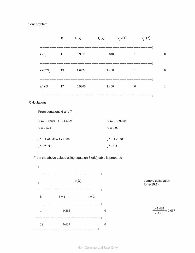
In our problem

k R(k) Q(k) ⋅vk

((1)) ⋅vk

((2))

−−−−−−−−−−−−−−−−−−−−−−−−−−−−−−−−−−−−−−−−−−−−−−−−

CH3

1 0.9011 0.848 1 0

−−−−−−−−−−−−−−−−−−−−−−−−−−−−−−−−−−−−−−−−−−−−−−−−

COCH3

19 1.6724 1.488 1 0

−−−−−−−−−−−−−−−−−−−−−−−−−−−−−−−−−−−−−−−−−−−−−−−−

⋅H2O 17 0.9200 1.400 0 1

−−−−−−−−−−−−−−−−−−−−−−−−−−−−−−−−−−−−−−−−−−−−−−−−

Calculations

From equations 6 and 7

≔r1 +⋅1 0.9011 ⋅1 1.6724 ≔r2 ⋅1 0.9200

=r1 2.574 =r2 0.92

≔q1 +⋅1 0.848 ⋅1 1.488 ≔q2 ⋅1 1.400

=q1 2.336 =q2 1.4

From the above values using equation 8 e(ki) table is prepared

−

−−−−−−−−−−−−−−−−−−−−−−−−−−−

e ((ki)) sample calculation for e(19,1)−

−−−−−−−−−−−−−−−−−−−−−−−−−−−

k i = 1 i = 2

−−−−−−−−−−−−−−−−−−−−−−−−−−−−

1 0.363 0 =―――⋅1 1.488

2.3360.637

−−−−−−−−−−−−−−−−−−−−−−−−−−−−

19 0.637 0

−−−−−−−−−−−−−−−−−−−−−−−−−−−−


−−−−−−−−−−−−−−−−−−−−−−−−−−−−

17 0 1

−−−−−−−−−−−−−−−−−−−−−−−−−−−−

Interaction parameters from tables

＝＝＝a (( ,1 1)) a (( ,19 19)) a (( ,17 17)) 0

＝a (( ,1 19)) 476.4 ＝a (( ,19 1)) 26.76

＝a (( ,1 17)) 1318.00 ＝a (( ,17 1)) 300.00

＝a (( ,19 17)) 472.50 ＝a (( ,17 19)) −195.40

≡bar ⋅105 Pa ≔Rgas ⋅8.314 ―――joule

⋅mole K

acetone ---- 1water ---- 2

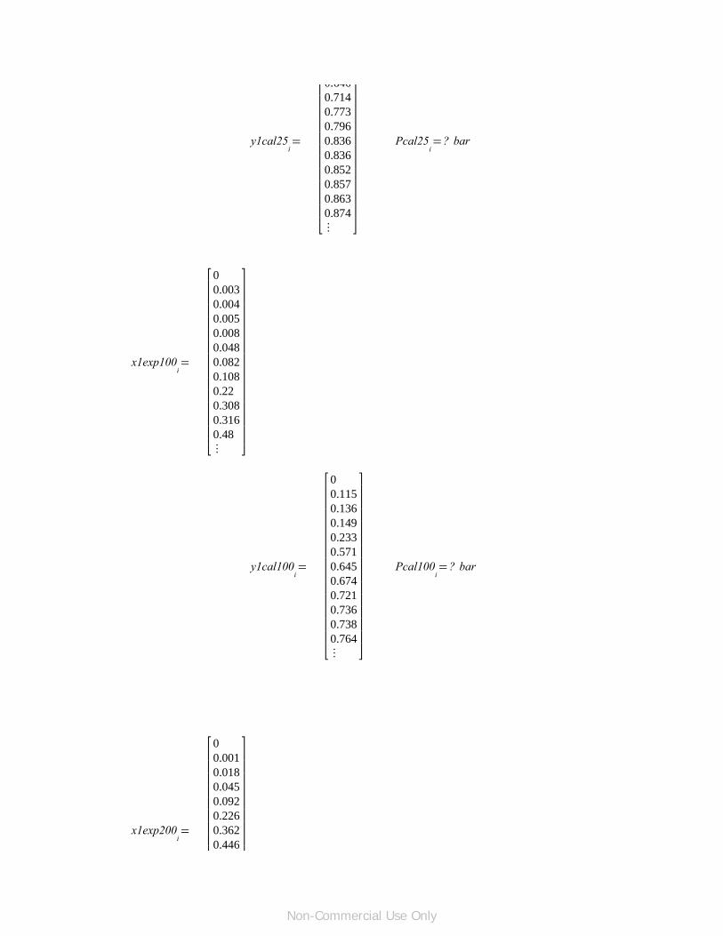
Experimental values of liquid phase composition (x1exp25), vapor phase composition (y1exp25) of acetone and total pressure of the system are given as shown below.

At 25C

≔i ‥0 16


≔x1exp25i

0.00000.00010.01940.02890.04490.05560.09390.09510.1310.1470.17910.26540.35380.58080.78520.99991.0000

⎡⎢⎢⎢⎢⎢⎢⎢⎢⎢⎢⎢⎢⎢⎢⎢⎢⎢⎢⎢⎣

⎤⎥⎥⎥⎥⎥⎥⎥⎥⎥⎥⎥⎥⎥⎥⎥⎥⎥⎥⎥⎦

≔y1exp25i

0.00000.00010.52340.62120.71680.75910.83510.84160.86180.87680.87820.88560.89540.91580.94210.99991.0000

⎡⎢⎢⎢⎢⎢⎢⎢⎢⎢⎢⎢⎢⎢⎢⎢⎢⎢⎢⎢⎣

⎤⎥⎥⎥⎥⎥⎥⎥⎥⎥⎥⎥⎥⎥⎥⎥⎥⎥⎥⎥⎦

≔Pexp25i

⋅0.0314 bar⋅0.031597 bar⋅0.066795 bar⋅0.082393 bar⋅0.108391 bar⋅0.121457 bar⋅0.168120 bar⋅0.168786 bar⋅0.192384 bar⋅0.200784 bar⋅0.213049 bar⋅0.234781 bar⋅0.245847 bar⋅0.265445 bar⋅0.284643 bar⋅0.307856 bar⋅0.308000 bar

⎡⎢⎢⎢⎢⎢⎢⎢⎢⎢⎢⎢⎢⎢⎢⎢⎢⎢⎢⎢⎣

⎤⎥⎥⎥⎥⎥⎥⎥⎥⎥⎥⎥⎥⎥⎥⎥⎥⎥⎥⎥⎦

≔x2exp25i

−1 x1exp25iCalculation of activity coefficients by UNIFAC-method

≔r1 2.574 ≔r2 0.9200 From equations 6 and 7

≔q1 2.336 ≔q2 1.400

≔J1i

――――――――r1

+⋅r1 x1exp25i

⋅r2 x2exp25i

≔J2i

――――――――r2

+⋅r1 x1exp25i

⋅r2 x2exp25i

From equation 4

=J1i

2.7982.7972.7042.662.5892.5442.3942.3892.2652.2132.1161.894⋮

⎡⎢⎢⎢⎢⎢⎢⎢⎢⎢⎢⎢⎢⎢⎢⎣

⎤⎥⎥⎥⎥⎥⎥⎥⎥⎥⎥⎥⎥⎥⎥⎦

=J2i

110.9660.9510.9250.9090.8560.8540.8090.7910.7560.677⋮

⎡⎢⎢⎢⎢⎢⎢⎢⎢⎢⎢⎢⎢⎢⎢⎣

⎤⎥⎥⎥⎥⎥⎥⎥⎥⎥⎥⎥⎥⎥⎥⎦


≔L1i

――――――――q1

+⋅q1 x1exp25i

⋅q2 x2exp25i

≔L2i

――――――――q2

+⋅q1 x1exp25i

⋅q2 x2exp25i

From equation 5

=L1i

1.6691.6681.6471.6371.621.6091.571.5691.5341.5191.491.417⋮

⎡⎢⎢⎢⎢⎢⎢⎢⎢⎢⎢⎢⎢⎢⎢⎣

⎤⎥⎥⎥⎥⎥⎥⎥⎥⎥⎥⎥⎥⎥⎥⎦

=L2i

110.9870.9810.9710.9640.9410.940.9190.9110.8930.849⋮

⎡⎢⎢⎢⎢⎢⎢⎢⎢⎢⎢⎢⎢⎢⎢⎣

⎤⎥⎥⎥⎥⎥⎥⎥⎥⎥⎥⎥⎥⎥⎥⎦

⋅⋅x1exp25 q1 0.363


≔θ1i

――――――――⋅⋅x1exp25

iq1 0.363

+⋅x1exp25iq1 ⋅x2exp25

iq2 ≔θ19

i――――――――

⋅⋅x1exp25iq1 0.637


iq2

≔θ17i

――――――――⋅⋅x2exp25

iq2 1


iq2

From equation 9

=θ17i

110.9680.9530.9270.9110.8530.8510.7990.7770.7330.624⋮

⎡⎢⎢⎢⎢⎢⎢⎢⎢⎢⎢⎢⎢⎢⎢⎣

⎤⎥⎥⎥⎥⎥⎥⎥⎥⎥⎥⎥⎥⎥⎥⎦

=θ1i

0⋅6.057 10−5

0.0120.0170.0260.0320.0540.0540.0730.0810.0970.137⋮

⎡⎢⎢⎢⎢⎢⎢⎢⎢⎢⎢⎢⎢⎢⎢⎣

⎤⎥⎥⎥⎥⎥⎥⎥⎥⎥⎥⎥⎥⎥⎥⎦

=θ19i

0⋅1.063 10−4

0.020.030.0460.0570.0940.0950.1280.1420.170.24⋮

⎡⎢⎢⎢⎢⎢⎢⎢⎢⎢⎢⎢⎢⎢⎢⎣

⎤⎥⎥⎥⎥⎥⎥⎥⎥⎥⎥⎥⎥⎥⎥⎦

From equation 10

τ ((mk)) 's in equation 10 are calculated from equation 11

≔s1i

++⋅θ1i

1 ⋅θ19i

0.914 ⋅θ17i

0.365

Sample calculation

≔s19i

++⋅θ1i

0.202 ⋅θ19i

1 ⋅θ17i

1.926

＝τ (( ,1 19))

=exp⎛⎜⎝―――−476.4

298

⎞⎟⎠

0.202

≔s17i

++⋅θ1i

0.012 ⋅θ19i

0.205 ⋅θ17i

1


=s1i

0.3650.3650.3840.3920.4070.4170.4510.4520.4820.4950.520.583⋮

⎡⎢⎢⎢⎢⎢⎢⎢⎢⎢⎢⎢⎢⎢⎢⎣

⎤⎥⎥⎥⎥⎥⎥⎥⎥⎥⎥⎥⎥⎥⎥⎦

=s19i

1.9261.9261.8871.8681.8381.8171.7471.7451.6821.6551.6021.469⋮

⎡⎢⎢⎢⎢⎢⎢⎢⎢⎢⎢⎢⎢⎢⎢⎣

⎤⎥⎥⎥⎥⎥⎥⎥⎥⎥⎥⎥⎥⎥⎥⎦

=s17i

110.9720.9590.9370.9230.8720.8710.8260.8070.7690.675⋮

⎡⎢⎢⎢⎢⎢⎢⎢⎢⎢⎢⎢⎢⎢⎢⎣

⎤⎥⎥⎥⎥⎥⎥⎥⎥⎥⎥⎥⎥⎥⎥⎦

≔lnγc1i

−+−1 J1iln ⎛

⎝J1i⎞⎠

⋅⋅5 q1

⎛⎜⎜⎜⎝

+−1 ――J1i

L1i

ln

⎛⎜⎜⎜⎝

――J1i

L1i

⎞⎟⎟⎟⎠

⎞⎟⎟⎟⎠

From equation 2

≔lnγc2i

−+−1 J2iln ⎛

⎝J2i⎞⎠

⋅⋅5 q2

⎛⎜⎜⎜⎝

+−1 ――J2i

L2i

ln

⎛⎜⎜⎜⎝

――J2i

L2i

⎞⎟⎟⎟⎠

⎞⎟⎟⎟⎠

⎛ ⎛⎛ 0.945 ⎛ 0.945 ⎞⎞ ⎛ 0.71 ⎛ 0.71 ⎞⎞ ⎛ 0.135 ⎞⎞⎞


≔lnγr1i

⋅q1⎛⎜⎜⎝

−1⎛⎜⎜⎝

++⎛⎜⎜⎝

−⋅θ1i

――0.945

s1i

⋅0.363 ln⎛⎜⎜⎝

――0.945

s1i

⎞⎟⎟⎠

⎞⎟⎟⎠

⎛⎜⎜⎝

−⋅θ19i

――0.71

s19i

⋅0.637 ln⎛⎜⎜⎝

――0.71

s19i

⎞⎟⎟⎠

⎞⎟⎟⎠

⎛⎜⎜⎝

⋅θ17i

――0.135

s17i

⎞⎟⎟⎠

⎞⎟⎟⎠

⎞⎟⎟⎠

From equation 3

≔lnγr2i

⋅q2⎛⎜⎜⎝

−1⎛⎜⎜⎝

++⎛⎜⎜⎝

⋅θ1i

――0.365

s1i

⎞⎟⎟⎠

⎛⎜⎜⎝

⋅θ19i

――1.926

s19i

⎞⎟⎟⎠

⎛⎜⎜⎝

−⋅θ17i

――1

s17i

ln⎛⎜⎜⎝

――1

s17i

⎞⎟⎟⎠

⎞⎟⎟⎠

⎞⎟⎟⎠

⎞⎟⎟⎠

β ((ik)) 's are calculated by equation 12.

sample calculation

＝β (( ,1 19))

=+⋅0.363 0.202 ⋅0.637 1 0.71

=lnγr1i

1.3421.3421.2471.2051.1381.0960.9650.9610.8590.8180.7440.585⋮

⎡⎢⎢⎢⎢⎢⎢⎢⎢⎢⎢⎢⎢⎢⎢⎣

⎤⎥⎥⎥⎥⎥⎥⎥⎥⎥⎥⎥⎥⎥⎥⎦

=lnγr2i

0⋅2.594 10−8

⋅9.15 10−4

0.0020.0050.0070.0170.0180.0310.0370.0520.097⋮

⎡⎢⎢⎢⎢⎢⎢⎢⎢⎢⎢⎢⎢⎢⎢⎣

⎤⎥⎥⎥⎥⎥⎥⎥⎥⎥⎥⎥⎥⎥⎥⎦

=lnγc1i

1.0991.0980.9940.9470.8720.8260.6810.6770.5650.5220.4440.287⋮

⎡⎢⎢⎢⎢⎢⎢⎢⎢⎢⎢⎢⎢⎢⎢⎣

⎤⎥⎥⎥⎥⎥⎥⎥⎥⎥⎥⎥⎥⎥⎥⎦

=lnγc2i

0⋅2.846 10−8

0.0010.0020.0050.0070.0190.020.0340.0410.0560.1⋮

⎡⎢⎢⎢⎢⎢⎢⎢⎢⎢⎢⎢⎢⎢⎢⎣

⎤⎥⎥⎥⎥⎥⎥⎥⎥⎥⎥⎥⎥⎥⎥⎦

≔γ1iexp ⎛

⎝+lnγc1ilnγr1

i⎞⎠

≔γ2iexp ⎛

⎝+lnγc2ilnγr2

i⎞⎠

=γ1i

11.48511.4739.4078.5977.4666.8385.1855 145

⎡⎢⎢⎢⎢⎢⎢⎢⎢

⎤⎥⎥⎥⎥⎥⎥⎥⎥

=γ2i

111.0021.0041.011.0141.0371 038

⎡⎢⎢⎢⎢⎢⎢⎢⎢

⎤⎥⎥⎥⎥⎥⎥⎥⎥


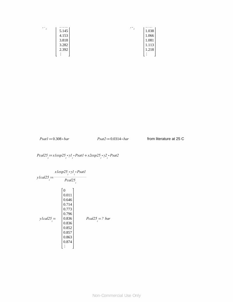
γ1i

5.1855.1454.1533.8183.2822.392⋮

⎢⎢⎢⎢⎢⎢⎢⎣

⎥⎥⎥⎥⎥⎥⎥⎦

γ2i

1.0371.0381.0661.0811.1131.218⋮

⎢⎢⎢⎢⎢⎢⎢⎣

⎥⎥⎥⎥⎥⎥⎥⎦

≔Psat1 ⋅0.308 bar ≔Psat2 ⋅0.0314 bar from literature at 25 C

≔Pcal25i

+⋅⋅x1exp25iγ1iPsat1 ⋅⋅x2exp25

iγ2iPsat2

≔y1cal25i

――――――⋅⋅x1exp25

iγ1iPsat1

Pcal25i

=y1cal25i

00.0110.6460.7140.7730.7960.8360.8360.8520.8570.8630.874⋮

⎡⎢⎢⎢⎢⎢⎢⎢⎢⎢⎢⎢⎢⎢⎢⎣

⎤⎥⎥⎥⎥⎥⎥⎥⎥⎥⎥⎥⎥⎥⎥⎦

=Pcal25i? bar


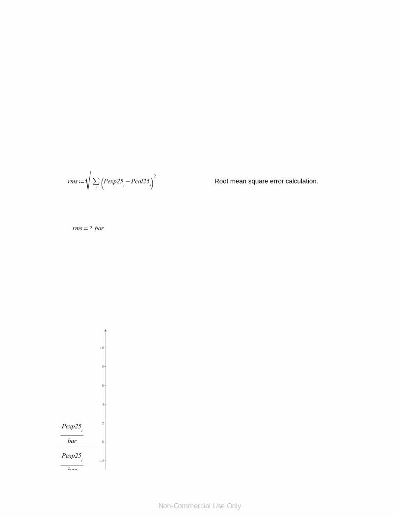
≔rms‾‾‾‾‾‾‾‾‾‾‾‾‾‾‾‾‾∑i

⎛⎝

−Pexp25iPcal25

i⎞⎠

2

Root mean square error calculation.

=rms ? bar

-2

0

2

4

6

8

10

―――Pexp25

i

bar

―――Pexp25

i

bar


-6

-4

-10

-8

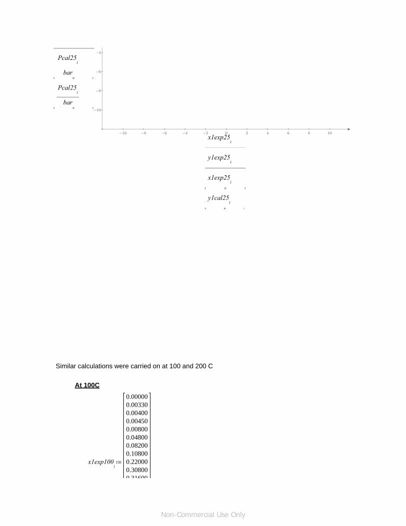
-6 -4 -2 0 2 4 6 8-10 -8 10

―――Pcal25

i

bar

―――Pcal25

i

bar

x1exp25i

y1exp25i

x1exp25i

y1cal25i

Similar calculations were carried on at 100 and 200 C

At 100C

≔x1exp100i

0.000000.003300.004000.004500.008000.048000.082000.108000.220000.308000 31600

⎡⎢⎢⎢⎢⎢⎢⎢⎢⎢⎢⎢⎢

⎤⎥⎥⎥⎥⎥⎥⎥⎥⎥⎥⎥⎥


0.480000.695000.742000.854000.971001.00000

⎢⎢⎢⎢⎢⎢⎢⎣

⎥⎥⎥⎥⎥⎥⎥⎦

≔y1exp100i

0.000000.090200.109000.118000.207000.545000.613000.632000.705000.715000.719000.747000.801000.823000.878000.972001.00000

⎡⎢⎢⎢⎢⎢⎢⎢⎢⎢⎢⎢⎢⎢⎢⎢⎢⎢⎢⎢⎣

⎤⎥⎥⎥⎥⎥⎥⎥⎥⎥⎥⎥⎥⎥⎥⎥⎥⎥⎥⎥⎦

≔Pexp100i

⋅1.013000 bar⋅1.110056 bar⋅1.130734 bar⋅1.145439 bar⋅1.303107 bar⋅2.240790 bar⋅2.447639 bar⋅2.785478 bar⋅3.068162 bar⋅3.199164 bar⋅3.206057 bar⋅3.474955 bar⋅3.571481 bar⋅3.599065 bar⋅3.674899 bar⋅3.681805 bar⋅3.722000 bar

⎡⎢⎢⎢⎢⎢⎢⎢⎢⎢⎢⎢⎢⎢⎢⎢⎢⎢⎢⎢⎣

⎤⎥⎥⎥⎥⎥⎥⎥⎥⎥⎥⎥⎥⎥⎥⎥⎥⎥⎥⎥⎦

≔x2exp100i

−1 x1exp100i

≔r1 2.574 ≔r2 0.9200

≔q1 2.336 ≔q2 1.400

≔J1i

―――――――――r1

+⋅r1 x1exp100i

⋅r2 x2exp100i

≔J2i

―――――――――r2

+⋅r1 x1exp100i

⋅r2 x2exp100i

=J1i

2.7982.7812.7782.7752.7582.5762.4382.3432.0051.8011.7841.502⋮

⎡⎢⎢⎢⎢⎢⎢⎢⎢⎢⎢⎢⎢⎢⎢⎣

⎤⎥⎥⎥⎥⎥⎥⎥⎥⎥⎥⎥⎥⎥⎥⎦

=J2i

10.9940.9930.9920.9860.9210.8720.8370.7170.6440.6380.537⋮

⎡⎢⎢⎢⎢⎢⎢⎢⎢⎢⎢⎢⎢⎢⎢⎣

⎤⎥⎥⎥⎥⎥⎥⎥⎥⎥⎥⎥⎥⎥⎥⎦


≔L1i

―――――――――q1

+⋅q1 x1exp100i

⋅q2 x2exp100i

≔L2i

―――――――――q2

+⋅q1 x1exp100i

⋅q2 x2exp100i

=L1i

1.6691.6651.6641.6641.661.6171.5821.5561.4551.3841.3781.263⋮

⎡⎢⎢⎢⎢⎢⎢⎢⎢⎢⎢⎢⎢⎢⎢⎣

⎤⎥⎥⎥⎥⎥⎥⎥⎥⎥⎥⎥⎥⎥⎥⎦

=L2i

10.9980.9970.9970.9950.9690.9480.9330.8720.8290.8260.757⋮

⎡⎢⎢⎢⎢⎢⎢⎢⎢⎢⎢⎢⎢⎢⎢⎣

⎤⎥⎥⎥⎥⎥⎥⎥⎥⎥⎥⎥⎥⎥⎥⎦


≔θ1i

―――――――――⋅⋅x1exp100

iq1 0.363


iq2

≔θ19i

―――――――――⋅⋅x1exp100

iq1 0.637


iq2

≔θ17i

―――――――――⋅x2exp100iq2


iq2

=θ1i

00.0020.0020.0030.0050.0280.0470.0610.1160.1550.1580.22⋮

⎡⎢⎢⎢⎢⎢⎢⎢⎢⎢⎢⎢⎢⎢⎢⎣

⎤⎥⎥⎥⎥⎥⎥⎥⎥⎥⎥⎥⎥⎥⎥⎦

=θ19i

00.0030.0040.0050.0080.0490.0830.1070.2040.2710.2770.386⋮

⎡⎢⎢⎢⎢⎢⎢⎢⎢⎢⎢⎢⎢⎢⎢⎣

⎤⎥⎥⎥⎥⎥⎥⎥⎥⎥⎥⎥⎥⎥⎥⎦

=θ17i

10.9950.9930.9930.9870.9220.870.8320.680.5740.5650.394⋮

⎡⎢⎢⎢⎢⎢⎢⎢⎢⎢⎢⎢⎢⎢⎢⎣

⎤⎥⎥⎥⎥⎥⎥⎥⎥⎥⎥⎥⎥⎥⎥⎦

≔s1i

++⋅θ1i

1 ⋅θ19i

0.9308 ⋅θ17i

0.4474

≔s19i

++⋅θ1i

0.2788 ⋅θ19i

1 ⋅θ17i

1.6885


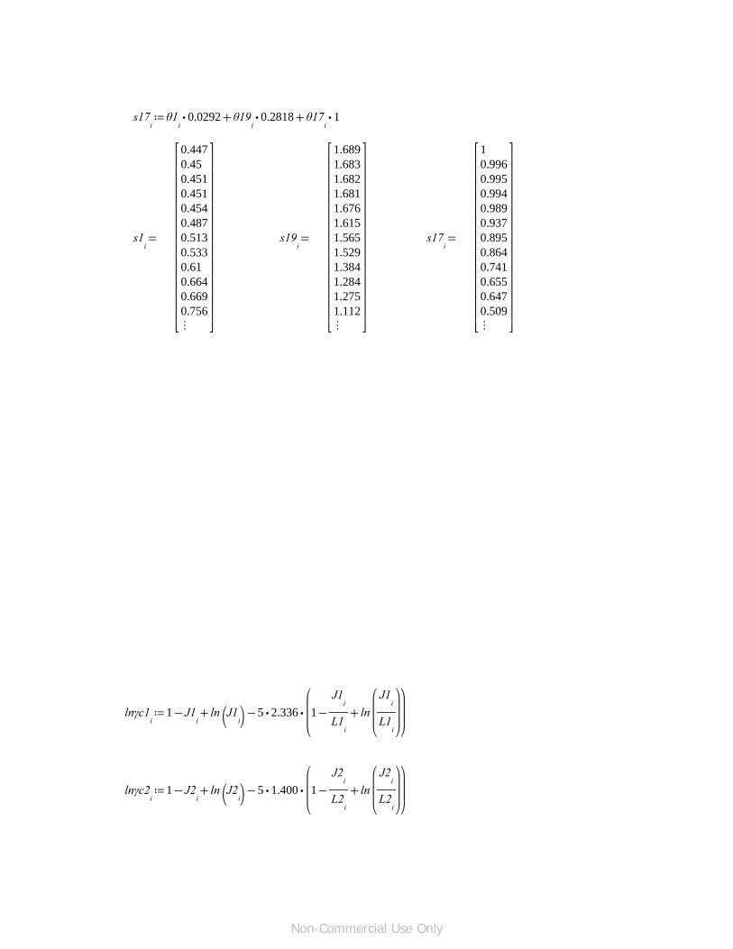
≔s17i

++⋅θ1i

0.0292 ⋅θ19i

0.2818 ⋅θ17i

1

=s1i

0.4470.450.4510.4510.4540.4870.5130.5330.610.6640.6690.756⋮

⎡⎢⎢⎢⎢⎢⎢⎢⎢⎢⎢⎢⎢⎢⎢⎣

⎤⎥⎥⎥⎥⎥⎥⎥⎥⎥⎥⎥⎥⎥⎥⎦

=s19i

1.6891.6831.6821.6811.6761.6151.5651.5291.3841.2841.2751.112⋮

⎡⎢⎢⎢⎢⎢⎢⎢⎢⎢⎢⎢⎢⎢⎢⎣

⎤⎥⎥⎥⎥⎥⎥⎥⎥⎥⎥⎥⎥⎥⎥⎦

=s17i

10.9960.9950.9940.9890.9370.8950.8640.7410.6550.6470.509⋮

⎡⎢⎢⎢⎢⎢⎢⎢⎢⎢⎢⎢⎢⎢⎢⎣

⎤⎥⎥⎥⎥⎥⎥⎥⎥⎥⎥⎥⎥⎥⎥⎦

≔lnγc1i

−+−1 J1iln ⎛

⎝J1i⎞⎠

⋅⋅5 2.336

⎛⎜⎜⎜⎝

+−1 ――J1i

L1i

ln

⎛⎜⎜⎜⎝

――J1i

L1i

⎞⎟⎟⎟⎠

⎞⎟⎟⎟⎠

≔lnγc2i

−+−1 J2iln ⎛

⎝J2i⎞⎠

⋅⋅5 1.400

⎛⎜⎜⎜⎝

+−1 ――J2i

L2i

ln

⎛⎜⎜⎜⎝

――J2i

L2i

⎞⎟⎟⎟⎠

⎞⎟⎟⎟⎠


≔lnγr1i

⋅q1⎛⎜⎜⎝

−1⎛⎜⎜⎝

++⎛⎜⎜⎝

−⋅θ1i

――0.956

s1i

⋅0.363 ln⎛⎜⎜⎝

――0.956

s1i

⎞⎟⎟⎠

⎞⎟⎟⎠

⎛⎜⎜⎝

−⋅θ19i

――0.738

s19i

⋅0.637 ln⎛⎜⎜⎝

――0.738

s19i

⎞⎟⎟⎠

⎞⎟⎟⎠

⎛⎜⎜⎝

⋅θ17i

――0.190

s17i

⎞⎟⎟⎠

⎞⎟⎟⎠

⎞⎟⎟⎠

≔lnγr2i

⋅q2⎛⎜⎜⎝

−1⎛⎜⎜⎝

++⎛⎜⎜⎝

⋅θ1i

―――0.4474

s1i

⎞⎟⎟⎠

⎛⎜⎜⎝

⋅θ19i

―――1.6885

s19i

⎞⎟⎟⎠

⎛⎜⎜⎝

−⋅θ17i

――1

s17i

ln⎛⎜⎜⎝

――1

s17i

⎞⎟⎟⎠

⎞⎟⎟⎠

⎞⎟⎟⎠

⎞⎟⎟⎠

=lnγc1i

1.0991.081.0761.0731.0540.8590.7230.6340.3620.2310.2220.09⋮

⎡⎢⎢⎢⎢⎢⎢⎢⎢⎢⎢⎢⎢⎢⎢⎣

⎤⎥⎥⎥⎥⎥⎥⎥⎥⎥⎥⎥⎥⎥⎥⎦

=lnγc2i

0⋅3.069 10−5

⋅4.5 10−5

⋅5.686 10−5

⋅1.778 10−4

0.0060.0150.0240.0760.1230.1270.211⋮

⎡⎢⎢⎢⎢⎢⎢⎢⎢⎢⎢⎢⎢⎢⎢⎣

⎤⎥⎥⎥⎥⎥⎥⎥⎥⎥⎥⎥⎥⎥⎥⎦

=lnγr1i

1.3041.2911.2881.2861.2721.1241.0170.9440.6940.5480.5360.333⋮

⎡⎢⎢⎢⎢⎢⎢⎢⎢⎢⎢⎢⎢⎢⎢⎣

⎤⎥⎥⎥⎥⎥⎥⎥⎥⎥⎥⎥⎥⎥⎥⎦

=lnγr2i

0⋅2.257 10−5

⋅3.31 10−5

⋅4.184 10−5

⋅1.311 10−4

0.0040.0120.0190.0680.120.1250.259⋮

⎡⎢⎢⎢⎢⎢⎢⎢⎢⎢⎢⎢⎢⎢⎢⎣

⎤⎥⎥⎥⎥⎥⎥⎥⎥⎥⎥⎥⎥⎥⎥⎦

≔γ1iexp ⎛

⎝+lnγc1ilnγr1

i⎞⎠

≔γ2iexp ⎛

⎝+lnγc2ilnγr2

i⎞⎠

=γ1

11.05810.70710.63410.58310.2357.2655.697

⎡⎢⎢⎢⎢⎢⎢⎢⎢

⎤⎥⎥⎥⎥⎥⎥⎥⎥

=γ2

111111.011.027

⎡⎢⎢⎢⎢⎢⎢⎢⎢

⎤⎥⎥⎥⎥⎥⎥⎥⎥


=γ1i

5.6974.8472.8752.1782.1331.526⋮

⎢⎢⎢⎢⎢⎢⎢⎢⎣

⎥⎥⎥⎥⎥⎥⎥⎥⎦

=γ2i

1.0271.0451.1551.2751.2871.601⋮

⎢⎢⎢⎢⎢⎢⎢⎢⎣

⎥⎥⎥⎥⎥⎥⎥⎥⎦

≔Psat1 ⋅3.722 bar ≔Psat2 ⋅1.013 bar

≔Pcal100i


iγ2iPsat2

≔y1cal100i

――――――⋅⋅x1exp100

iγ1iPsat1

Pcal100i

=y1cal100i

00.1150.1360.1490.2330.5710.6450.6740.7210.7360.7380.764⋮

⎡⎢⎢⎢⎢⎢⎢⎢⎢⎢⎢⎢⎢⎢⎢⎣

⎤⎥⎥⎥⎥⎥⎥⎥⎥⎥⎥⎥⎥⎥⎥⎦

=Pcal100i? bar


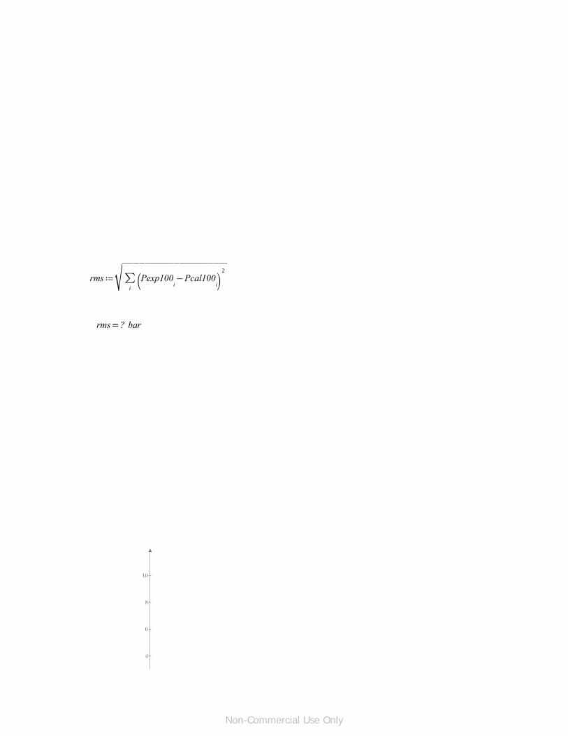
≔rms‾‾‾‾‾‾‾‾‾‾‾‾‾‾‾‾‾‾‾∑i

⎛⎝

−Pexp100iPcal100

i⎞⎠

2

=rms ? bar

4

6

8

10


-6

-4

-2

0

2

-10

-8

-6 -4 -2 0 2 4 6 8-10 -8 10

―――Pexp100

i

bar

―――Pexp100

i

bar

―――Pcal100

i

bar

―――Pcal100

i

bar

x1exp100i

y1exp100i

x1exp100i

y1cal100i

At 200C

≔x1exp200i

0.00000.00130.01820.04500.09200.22600.36200.44600.55100.65900 7580

⎡⎢⎢⎢⎢⎢⎢⎢⎢⎢⎢⎢⎢

⎤⎥⎥⎥⎥⎥⎥⎥⎥⎥⎥⎥⎥

≔y1exp200i

0.00000.01600.13600.26800.35400.45500.50200.54000.59500.66500 7430

⎡⎢⎢⎢⎢⎢⎢⎢⎢⎢⎢⎢⎢

⎤⎥⎥⎥⎥⎥⎥⎥⎥⎥⎥⎥⎥

≔Pexp200i

⋅15.552476 bar⋅15.995808 bar⋅18.202126 bar⋅21.511604 bar⋅24.200554 bar⋅27.303190 bar⋅28.751086 bar⋅29.440560 bar⋅30.267930 bar⋅30.543720 bar⋅30 336877 bar

⎡⎢⎢⎢⎢⎢⎢⎢⎢⎢⎢⎢⎢

⎤⎥⎥⎥⎥⎥⎥⎥⎥⎥⎥⎥⎥


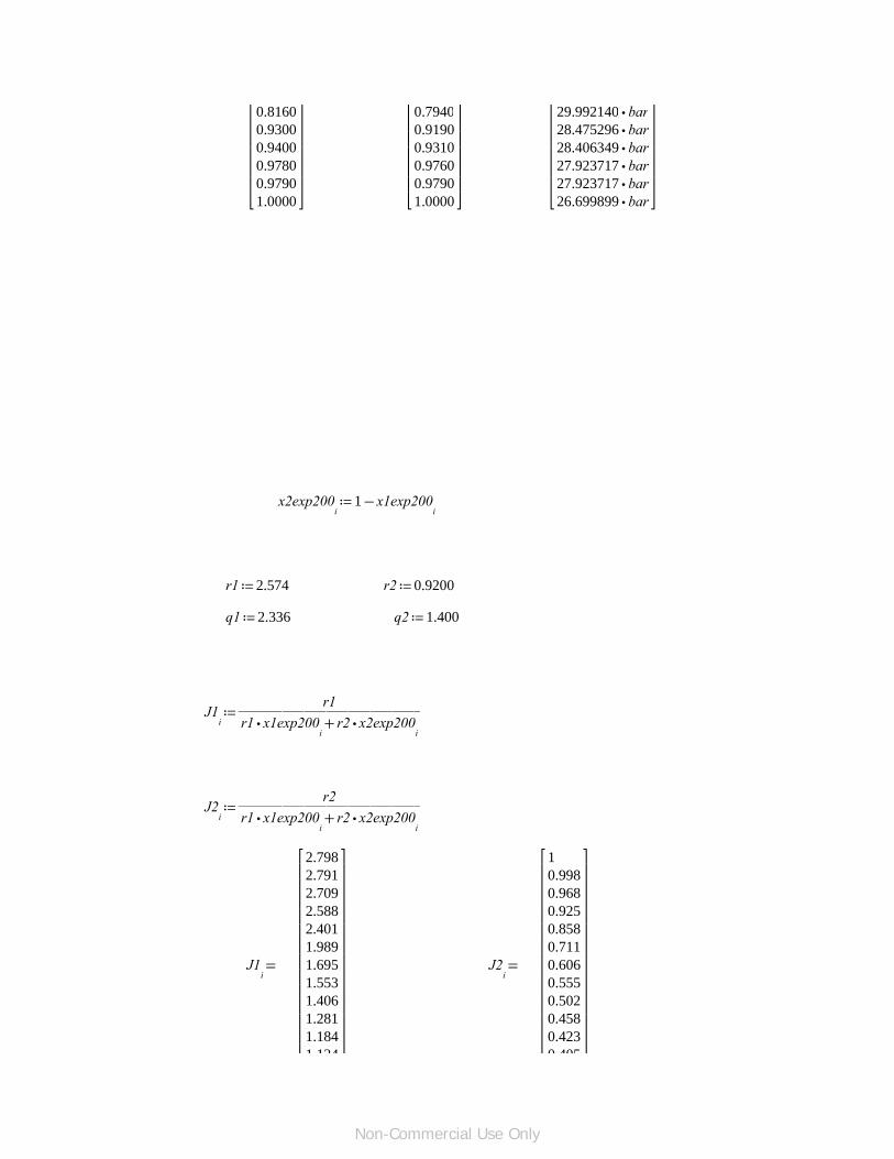
0.81600.93000.94000.97800.97901.0000

⎢⎢⎢⎢⎢⎢⎢⎣

⎥⎥⎥⎥⎥⎥⎥⎦

0.79400.91900.93100.97600.97901.0000

⎢⎢⎢⎢⎢⎢⎢⎣

⎥⎥⎥⎥⎥⎥⎥⎦

⋅29.992140 bar⋅28.475296 bar⋅28.406349 bar⋅27.923717 bar⋅27.923717 bar⋅26.699899 bar

⎢⎢⎢⎢⎢⎢⎢⎣

⎥⎥⎥⎥⎥⎥⎥⎦

≔x2exp200i

−1 x1exp200i

≔r1 2.574 ≔r2 0.9200

≔q1 2.336 ≔q2 1.400

≔J1i

―――――――――r1

+⋅r1 x1exp200i

⋅r2 x2exp200i

≔J2i

―――――――――r2

+⋅r1 x1exp200i

⋅r2 x2exp200i

=J1i

2.7982.7912.7092.5882.4011.9891.6951.5531.4061.2811.1841 134

⎡⎢⎢⎢⎢⎢⎢⎢⎢⎢⎢⎢⎢⎢

⎤⎥⎥⎥⎥⎥⎥⎥⎥⎥⎥⎥⎥⎥

=J2i

10.9980.9680.9250.8580.7110.6060.5550.5020.4580.4230 405

⎡⎢⎢⎢⎢⎢⎢⎢⎢⎢⎢⎢⎢⎢

⎤⎥⎥⎥⎥⎥⎥⎥⎥⎥⎥⎥⎥⎥


⋮⎢⎣ ⎥⎦ ⋮⎢⎣ ⎥⎦

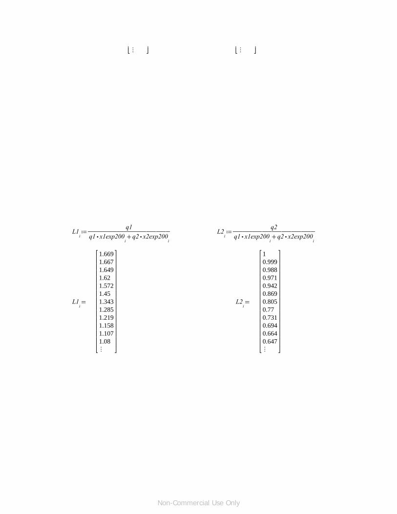
≔L1i

―――――――――q1

+⋅q1 x1exp200i

⋅q2 x2exp200i

≔L2i

―――――――――q2

+⋅q1 x1exp200i

⋅q2 x2exp200i

=L1i

1.6691.6671.6491.621.5721.451.3431.2851.2191.1581.1071.08⋮

⎡⎢⎢⎢⎢⎢⎢⎢⎢⎢⎢⎢⎢⎢⎢⎣

⎤⎥⎥⎥⎥⎥⎥⎥⎥⎥⎥⎥⎥⎥⎥⎦

=L2i

10.9990.9880.9710.9420.8690.8050.770.7310.6940.6640.647⋮

⎡⎢⎢⎢⎢⎢⎢⎢⎢⎢⎢⎢⎢⎢⎢⎣

⎤⎥⎥⎥⎥⎥⎥⎥⎥⎥⎥⎥⎥⎥⎥⎦


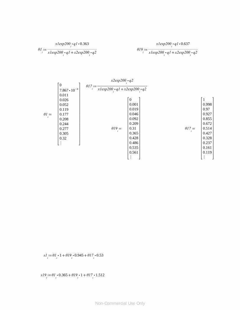
≔θ1i

―――――――――⋅⋅x1exp200

iq1 0.363


iq2

≔θ19i

―――――――――⋅⋅x1exp200

iq1 0.637


iq2

≔θ17i

―――――――――⋅x2exp200iq2


iq2

=θ1i

0⋅7.867 10−4

0.0110.0260.0520.1190.1770.2080.2440.2770.3050.32⋮

⎡⎢⎢⎢⎢⎢⎢⎢⎢⎢⎢⎢⎢⎢⎢⎣

⎤⎥⎥⎥⎥⎥⎥⎥⎥⎥⎥⎥⎥⎥⎥⎦

=θ19i

00.0010.0190.0460.0920.2090.310.3650.4280.4860.5350.561⋮

⎡⎢⎢⎢⎢⎢⎢⎢⎢⎢⎢⎢⎢⎢⎢⎣

⎤⎥⎥⎥⎥⎥⎥⎥⎥⎥⎥⎥⎥⎥⎥⎦

=θ17i

10.9980.970.9270.8550.6720.5140.4270.3280.2370.1610.119⋮

⎡⎢⎢⎢⎢⎢⎢⎢⎢⎢⎢⎢⎢⎢⎢⎣

⎤⎥⎥⎥⎥⎥⎥⎥⎥⎥⎥⎥⎥⎥⎥⎦

≔s1i

++⋅θ1i

1 ⋅θ19i

0.945 ⋅θ17i

0.53

≔s19i

++⋅θ1i

0.365 ⋅θ19i

1 ⋅θ17i

1.512


≔s17i

++⋅θ1i

0.062 ⋅θ19i

0.368 ⋅θ17i

1

=s1i

0.530.5310.5430.5620.5930.6720.7420.7790.8220.8620.8950.913⋮

⎡⎢⎢⎢⎢⎢⎢⎢⎢⎢⎢⎢⎢⎢⎢⎣

⎤⎥⎥⎥⎥⎥⎥⎥⎥⎥⎥⎥⎥⎥⎥⎦

=s19i

1.5121.511.491.4581.4051.2691.1511.0861.0130.9450.8890.858⋮

⎡⎢⎢⎢⎢⎢⎢⎢⎢⎢⎢⎢⎢⎢⎢⎣

⎤⎥⎥⎥⎥⎥⎥⎥⎥⎥⎥⎥⎥⎥⎥⎦

=s17i

10.9980.9780.9460.8930.7570.6390.5740.5010.4330.3760.345⋮

⎡⎢⎢⎢⎢⎢⎢⎢⎢⎢⎢⎢⎢⎢⎢⎣

⎤⎥⎥⎥⎥⎥⎥⎥⎥⎥⎥⎥⎥⎥⎥⎦

≔lnγc1i

−+−1 J1iln ⎛

⎝J1i⎞⎠

⋅⋅5 2.336

⎛⎜⎜⎜⎝

+−1 ――J1i

L1i

ln

⎛⎜⎜⎜⎝

――J1i

L1i

⎞⎟⎟⎟⎠

⎞⎟⎟⎟⎠

≔lnγc2i

−+−1 J2iln ⎛

⎝J2i⎞⎠

⋅⋅5 1.400

⎛⎜⎜⎜⎝

+−1 ――J2i

L2i

ln

⎛⎜⎜⎜⎝

――J2i

L2i

⎞⎟⎟⎟⎠

⎞⎟⎟⎟⎠


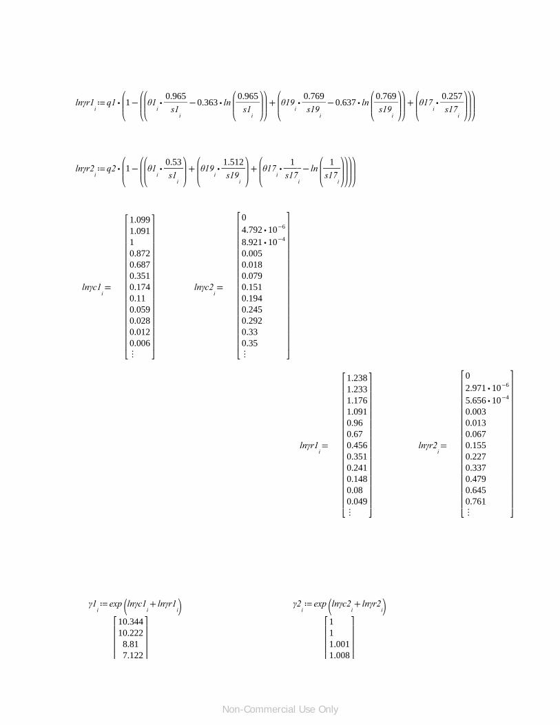
≔lnγr1i

⋅q1⎛⎜⎜⎝

−1⎛⎜⎜⎝

++⎛⎜⎜⎝

−⋅θ1i

――0.965

s1i

⋅0.363 ln⎛⎜⎜⎝

――0.965

s1i

⎞⎟⎟⎠

⎞⎟⎟⎠

⎛⎜⎜⎝

−⋅θ19i

――0.769

s19i

⋅0.637 ln⎛⎜⎜⎝

――0.769

s19i

⎞⎟⎟⎠

⎞⎟⎟⎠

⎛⎜⎜⎝

⋅θ17i

――0.257

s17i

⎞⎟⎟⎠

⎞⎟⎟⎠

⎞⎟⎟⎠

≔lnγr2i

⋅q2⎛⎜⎜⎝

−1⎛⎜⎜⎝

++⎛⎜⎜⎝

⋅θ1i

――0.53

s1i

⎞⎟⎟⎠

⎛⎜⎜⎝

⋅θ19i

――1.512

s19i

⎞⎟⎟⎠

⎛⎜⎜⎝

−⋅θ17i

――1

s17i

ln⎛⎜⎜⎝

――1

s17i

⎞⎟⎟⎠

⎞⎟⎟⎠

⎞⎟⎟⎠

⎞⎟⎟⎠

=lnγc1i

1.0991.09110.8720.6870.3510.1740.110.0590.0280.0120.006⋮

⎡⎢⎢⎢⎢⎢⎢⎢⎢⎢⎢⎢⎢⎢⎢⎣

⎤⎥⎥⎥⎥⎥⎥⎥⎥⎥⎥⎥⎥⎥⎥⎦

=lnγc2i

0⋅4.792 10−6

⋅8.921 10−4

0.0050.0180.0790.1510.1940.2450.2920.330.35⋮

⎡⎢⎢⎢⎢⎢⎢⎢⎢⎢⎢⎢⎢⎢⎢⎣

⎤⎥⎥⎥⎥⎥⎥⎥⎥⎥⎥⎥⎥⎥⎥⎦

=lnγr1i

1.2381.2331.1761.0910.960.670.4560.3510.2410.1480.080.049⋮

⎡⎢⎢⎢⎢⎢⎢⎢⎢⎢⎢⎢⎢⎢⎢⎣

⎤⎥⎥⎥⎥⎥⎥⎥⎥⎥⎥⎥⎥⎥⎥⎦

=lnγr2i

0⋅2.971 10−6

⋅5.656 10−4

0.0030.0130.0670.1550.2270.3370.4790.6450.761⋮

⎡⎢⎢⎢⎢⎢⎢⎢⎢⎢⎢⎢⎢⎢⎢⎣

⎤⎥⎥⎥⎥⎥⎥⎥⎥⎥⎥⎥⎥⎥⎥⎦

≔γ1iexp ⎛

⎝+lnγc1ilnγr1

i⎞⎠

≔γ2iexp ⎛

⎝+lnγc2ilnγr2

i⎞⎠

10.34410.2228.817.122

⎡⎢⎢⎢⎢

⎤⎥⎥⎥⎥

111.0011.008

⎡⎢⎢⎢⎢

⎤⎥⎥⎥⎥


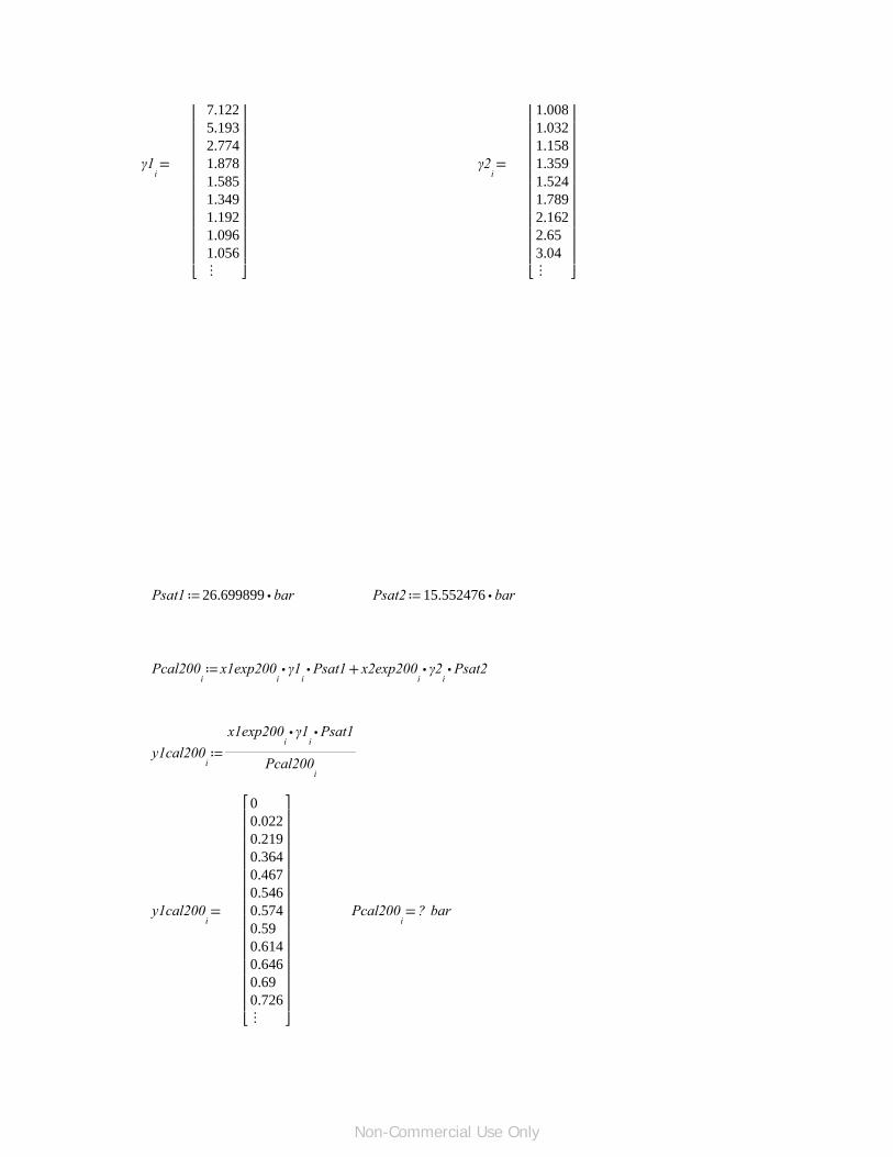
=γ1i

7.1225.1932.7741.8781.5851.3491.1921.0961.056⋮

⎢⎢⎢⎢⎢⎢⎢⎢⎢⎢⎢⎢⎣

⎥⎥⎥⎥⎥⎥⎥⎥⎥⎥⎥⎥⎦

=γ2i

1.0081.0321.1581.3591.5241.7892.1622.653.04⋮

⎢⎢⎢⎢⎢⎢⎢⎢⎢⎢⎢⎢⎣

⎥⎥⎥⎥⎥⎥⎥⎥⎥⎥⎥⎥⎦

≔Psat1 ⋅26.699899 bar ≔Psat2 ⋅15.552476 bar

≔Pcal200i


iγ2iPsat2

≔y1cal200i

――――――⋅⋅x1exp200

iγ1iPsat1

Pcal200i

=y1cal200i

00.0220.2190.3640.4670.5460.5740.590.6140.6460.690.726⋮

⎡⎢⎢⎢⎢⎢⎢⎢⎢⎢⎢⎢⎢⎢⎢⎣

⎤⎥⎥⎥⎥⎥⎥⎥⎥⎥⎥⎥⎥⎥⎥⎦

=Pcal200i? bar


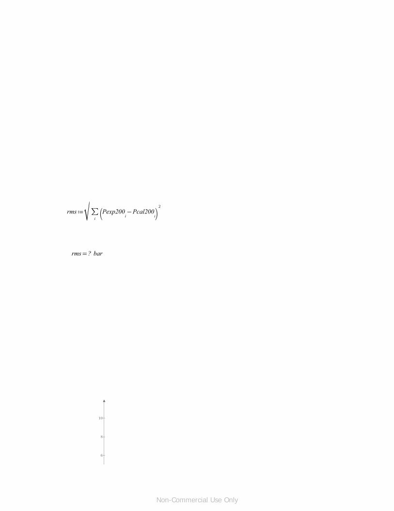
≔rms‾‾‾‾‾‾‾‾‾‾‾‾‾‾‾‾‾‾‾∑i

⎛⎝

−Pexp200iPcal200

i⎞⎠

2

=rms ? bar

6

8

10


-6

-4

-2

0

2

4

-10

-8

-6 -4 -2 0 2 4 6 8-10 -8 10

―――Pexp200

i

bar

―――Pexp200

i

bar

―――Pcal200

i

bar

―――Pcal200

i

bar

x1exp200i

y1exp200i

x1exp200i

y1cal200i

=x1exp25i

0⋅1 10−4

0.0190.0290.0450.0560.0940.0950.1310.1470.1790.265⋮

⎡⎢⎢⎢⎢⎢⎢⎢⎢⎢⎢⎢⎢⎢⎢⎣

⎤⎥⎥⎥⎥⎥⎥⎥⎥⎥⎥⎥⎥⎥⎥⎦

00.0110.6460 714

⎡⎢⎢⎢

⎤⎥⎥⎥


=y1cal25i

0.6460.7140.7730.7960.8360.8360.8520.8570.8630.874⋮

⎢⎢⎢⎢⎢⎢⎢⎢⎢⎢⎢⎢⎣

⎥⎥⎥⎥⎥⎥⎥⎥⎥⎥⎥⎥⎦

=Pcal25i? bar

=x1exp100i

00.0030.0040.0050.0080.0480.0820.1080.220.3080.3160.48⋮

⎡⎢⎢⎢⎢⎢⎢⎢⎢⎢⎢⎢⎢⎢⎢⎣

⎤⎥⎥⎥⎥⎥⎥⎥⎥⎥⎥⎥⎥⎥⎥⎦

=y1cal100i

00.1150.1360.1490.2330.5710.6450.6740.7210.7360.7380.764⋮

⎡⎢⎢⎢⎢⎢⎢⎢⎢⎢⎢⎢⎢⎢⎢⎣

⎤⎥⎥⎥⎥⎥⎥⎥⎥⎥⎥⎥⎥⎥⎥⎦

=Pcal100i? bar

=x1exp200i

00.0010.0180.0450.0920.2260.3620.446

⎡⎢⎢⎢⎢⎢⎢⎢⎢⎢

⎤⎥⎥⎥⎥⎥⎥⎥⎥⎥


0.5510.6590.7580.816⋮

⎢⎢⎢⎢⎢⎣

⎥⎥⎥⎥⎥⎦

=y1cal200i

00.0220.2190.3640.4670.5460.5740.590.6140.6460.690.726⋮

⎡⎢⎢⎢⎢⎢⎢⎢⎢⎢⎢⎢⎢⎢⎢⎣

⎤⎥⎥⎥⎥⎥⎥⎥⎥⎥⎥⎥⎥⎥⎥⎦

=Pcal200i? bar

≔Pcal augment (( ,,Pcal25 Pcal100 Pcal200))

=Pcal ? bar


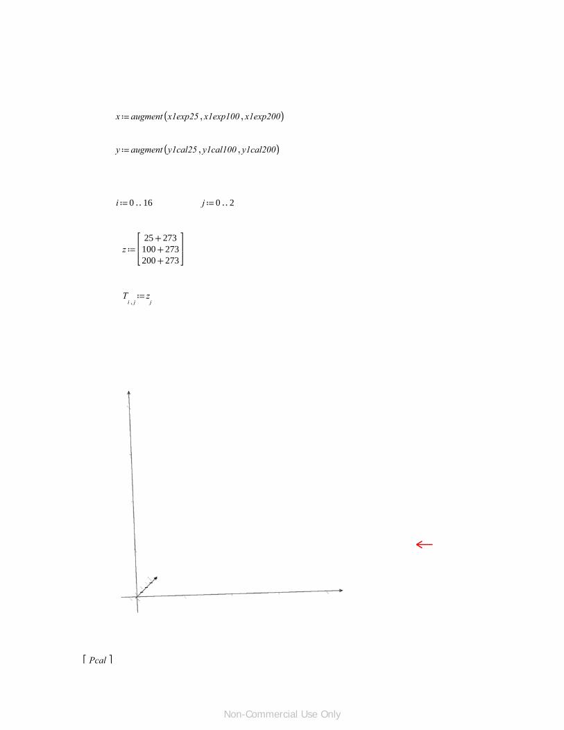
≔x augment (( ,,x1exp25 x1exp100 x1exp200))

≔y augment (( ,,y1cal25 y1cal100 y1cal200))

≔i ‥0 16 ≔j ‥0 2

≔z+25 273+100 273+200 273

⎡⎢⎢⎣

⎤⎥⎥⎦

≔T,i j

zj

Pcal⎡ ⎤


barxT

⎢⎢⎢⎣

⎥⎥⎥⎦

――Pcal

baryT

⎡⎢⎢⎢⎣

⎤⎥⎥⎥⎦

Conclusions

1) This metod is more accurate when compared to the other methods available.This can be seen by comparing the "root mean square" values of different methods with this method atsame temperature.

2) This method is most accurate at low temperatures.

3) This method doesn't require the knowledge of experimental values of x (liquid phasecomposition) and y (gas phase composition) to plot phase equilibrium plot. We can select our

own x values and find corresponding y values to construct phase equilibrium plot. The onlyvalues needed are the saturation pressures of the components which can be estimatedfrom Reidel corresponding states method.

4) This method doesn't require the knowledge of critical temperature and critical pressure values.

5) This method just requires the knowledge of structure of the compound to plot the phasediagrams of the compounds.Based on the structure, the compound is divided into subgroupsand calculations are performed.


plotting p-x-y diagram for binary system acetone/water at...

Documents