Playing Hard to Get: Strategic Misrepresentation

in Marriage Markets

Daniel Simundza∗†

July 14, 2015

Abstract

This paper presents a study of strategic interaction in marriage mar-kets, specifically the strategy known colloquially as “playing hard to get.”Even though the goal of playing hard to get is to misrepresent oneself, Ifind that the equilibrium response to this behavior actually results in amore efficient mating. In the model, agents observe noisy signals of po-tential mates’ types and have two chances to accept or reject a marriage.This modeling choice enables an agent to make initial strategic rejectionsin the hopes of improving her partner’s perception of her type. Previ-ous analyses of matching markets have not accounted for this behavior.I prove the existence of an equilibrium in which some low quality agentsplay hard to get by initially rejecting high signals. Despite this attempt atstrategic misrepresentation, I show that, relative to an equilibrium with-out any strategic behavior, mating is more efficient in the equilibrium withplaying hard to get.

Keywords: Matching; Misrepresentation; Search; Adverse selectionJEL Classification: D82, D83

∗I thank Hector Chade, Hans Haller, Ofer Setty, and Lones Smith for insightful discussionsand comments.†Contact: 3118 Pamplin Hall (0316), Blacksburg VA 24061, dan.simundza@gmail.com,

(540) 231 - 5764 Virginia Tech

1

Rule #5: Don’t call him and rarely return his calls.– The Rules: Time-Tested Secrets for Capturing the Heart of Mr.

Right by Ellen Fein & Sherrie Schneider

1 Introduction

In matching markets with private information over individual attributes, thedecision of whether to form a partnership may take place under significantuncertainty. Strategic behavior in such markets is therefore pervasive as agentsattempt to exploit their informational edge. This paper formalizes one particularstrategy, colloquially known as “playing hard to get,” in which agents initiallyconceal their interest in desirable partners in order to appear to be of a moredesirable type. I prove the existence of an equilibrium involving playing hardto get and show that mating remains positively assortative (i.e. people marryothers of similar type), a benchmark first established in Becker [1973], andrecently generalized to environments of incomplete information in Chade [2006].Moreover, I show that this sort of strategic behavior improves the sorting ofmates.

Previous frictional matching papers have modeled the “marry or not” de-cision as a one-shot game, and thus not accounted for strategic considerationswithin a relationship. In my model, agents have two chances to accept or re-ject a potential mate. This modeling choice enables an agent to make initialstrategic rejections in the hopes of improving her potential partner’s perceptionof her type.

In deciding whether to marry, agents judge the attractiveness of their currentpartner against the outside option of continuing to search for a better mate.1

When types are private information, agents do what they can to learn aboutpotential mates’ quality. Learning in relationships occurs not just through theobservation of noisy signals, but also by inferring type from behavior. Andwhile it may not be possible to alter one’s appearance or conversational ability,it is possible for the ordinary to behave as if they were extraordinary by playinghard to get.

In order to model this strategic behavior, I add dynamics to the pre-marriagerelationship. Specifically, matched agents observe noisy signals of each other’strue type and then have two “rounds” in which they can accept or reject amarriage. In equilibrium, agents’ first round announcements convey informationabout their type. Match partners must take this information into account whendetermining their second round announcement. Embedding this dynamic game

1Since my model is one in which utility is non-transferable (i.e. the quality of one’s matchpartner completely determines payoffs), I focus on social matching and the marriage market.If, alternatively, utility was transferable, all divorces would be mutually agreeable, which isclearly not the case. While strategic interaction is also likely to be important in the jobsearch setting and other situations in which the transferable utility assumption is reasonable,my assumption that utility is non-transferable rules out the possibility of side payments (e.g.wages) to facilitate matches. See McNamara and Collins [1990] and Moscarini [2005] for moreon search in labor markets.

2

in a marriage model allows low types to misrepresent themselves as high typesin hopes of marrying a better mate.

I show a Socially Strategic equilibrium exists in which some low type agentsplay hard to get by declining a match after observing an attractive signal inthe first round. If the agents do not form a marriage in the first round, theyupdate their beliefs as to their match partner’s type based on their first roundannouncements. In the Socially Strategic equilibrium, a positive fraction ofjilted high types who rejected their initially undesired partner change theirannouncement and optimally accept in the second round.

This behavior by the high types improves sorting by increasing the chancesthat a pair of high types marry in the event that they both send low signals.While the low types’ goal in playing hard to get is to increase mismatch, it is in-effective in equilibrium. I show that the Socially Strategic equilibrium increasessorting of types relative to an equilibrium without any strategic behavior.2

Despite the low types’ attempts at strategic misrepresentation, mating re-mains positively assortative in the Socially Strategic equilibrium. While hightypes who receive low signals mate with low types who receive high signals, theexpected partner of a high type agent is better than the expected partner of alow type agent.

In addition to establishing these results on the sorting and mating, I providecomparative statics results. I first focus on how the accuracy of the signalingtechnology, the fraction of high types in the population, the discount rate, thebaseline value of forming a match relative to remaining single, and the addedbenefit of marrying a high type affect the equilibrium behavior of the agents. Itis then straightforward to determine the effect of changes in these variables onthe set of matches that occur in equilibrium.

2 Related literature

In an early frictionless model, Becker [1973] established the allocative bench-mark of Positive Assortative Mating (PAM). He proved two results relevantfor the present study: first, PAM maximizes total output when types are pro-ductive complements, and second, PAM obtains in equilibrium when utility isnon-transferable and higher-type partners are more preferred.3 Smith [2006] ex-tended this framework to incorporate search frictions, and found that Becker’ssimple requirement that “higher is better” is insufficient to generate PAM whensearch takes time and agents are impatient. Instead, he showed that PAM ob-tains if the proportionate gains from mating with better partners are greaterfor high types than low.

2Damiano et al. [2005] study the allocative efficiency of dynamic matching markets inboth the presence and absence of participation costs. They show that, when there is no costof participation, the allocation achieved by the matching mechanism improves upon purelyrandom matching because high types match only with high types in early rounds. In contrast,my analysis takes place entirely in the steady state.

3See Consuegra et al. [2013] for a discussion of the necessity of the “higher is better”condition to generate PAM.

3

The first paper to incorporate information frictions into the searching andmatching framework was Chade [2006]. In his model, agents observe noisy sig-nals of their match-partner’s (private) type before deciding whether to marry.4

Chade [2006] proves the existence of an equilibrium in which “reservation sig-nals” characterize agents’ strategies, wherein agents accept only if the observedsignal exceeds a threshold which is increasing in the agent’s own type. Givensuch strategies, equilibrium matching is assortative on signals and, moreover,acceptance conveys bad news, a result the author terms the “acceptance curse.”

But if acceptance conveys bad news, then rejection makes the heart growfonder. To explain this point and to help motivate my model, consider a hightype man dating a high type woman who each, by chance, observe low signals.Further, suppose that the equilibrium strategies call for low types to acceptall signals and for high types to accept high signals and to reject low signals.5

After being rejected, our high type man and high type woman are each suretheir match parter was a high type, and would like to seek the other out andmate based on this revelation.

By adding within-match dynamics to the model, I not only allow agents topursue missed chances, I also allow others to take advantage of those who do.For if the high types in the above scenario take advantage of a second chance tomate, then low types observing high signals can guarantee themselves a marriagewith all partners by initially rejecting and then accepting.

My paper also contributes to a growing literature on matching markets withasymmetric information. One strand in this literature addresses moral hazard inmatching markets (see for example Wright [2004], Franco et al. [2011], and Serfes[2008]). Unlike the current paper, these studies describe types as commonlyobservable and actions as predictable given equilibrium incentives, so agentsdo not have uncertainty over payoffs or employ strategic behavior to improvepayoffs. The second strand is concerned with adverse selection, and includesInderst [2005] and Hopkins [2012]. While types are private information in thesepapers, the equilibria are “separating” – different types take different actions,and agents have no ex post uncertainty over type. I add to this literatureby analyzing a situation in which agents attempt to exploit their asymmetricinformation.

Psychologists, perhaps more than economists, have studied how and whyagents engage in strategic behavior while mating. Jonason and Li [2013] presentexperimental results on the tactics that agents use to play hard to get, how oftenmen and women use these tactics, and why they use them. One of their mostcommonly reported answers to the important question of “Why do you playhard to get?” was to increase demand.6 In fact, my model shows that while

4Anderson and Smith [2010] study matching with symmetric incomplete information aboutagent types and publicly observable joint production. They find conditions such that assor-tative matching on public reputation fails despite complementarities of production.

5Such a strategy profile is an equilibrium for intermediate discount rates in the binary typeand signal specialization in Section 4 of Chade [2006].

6The other most commonly reported answer was to test a potential mate’s level of com-mitment. While this is an interesting application of the strategy of playing hard to get, it is

4

playing hard to get can increase demand when one’s potential partner is initiallynot interested, it also derails some marriages with initially desirable and desiringpartners. The benefits of playing hard to get do not come without costs.

Strategic misrepresentation in stable matching mechanisms reflects a similartrade-off. Coles and Shorrer [2013] show that agents have incentives to truncatethe preference list they submit to the Deferred Acceptance Algorithm in order toincrease the expected value of being matched. Similar to the present paper, theirstudy shows that truncation increases payoffs conditional on a match occurring,but truncation also prevents the formation of some mutually beneficial matches.

The literature on “bluffing” in poker (Bellman and Blackwell [1949], Von Neu-mann and Morgenstern [1964]), wherein a player with a bad hand bids high, alsorelates to the present study. Von Neumann and Morgenstern [1964] cite two ben-efits of bluffing. The first is to induce opponents to believe one has a stronghand when it is in fact weak, thereby causing them to drop out. The second isto generate uncertainty, causing the opponent to stay in against a strong handat other points in the game. Only inducing opponents to believe a weak hand isactually strong relates to the motivation to play hard to get; the second benefitplays no role in my model because high types do not benefit from the addeduncertainty. Moreover, my focus is not just on why agents play hard to get, butalso on how this behavior affects mating.

3 Model

The main characteristics of the model are described below.Time: Time is discrete and is divided into periods of length equal to one.Agents: There is a continuum of male agents and a continuum of female

agents. The measure of each population is normalized to one. Each female ischaracterized by a type x ∈ L,H, and each male is characterized by a typey ∈ L,H, with 0 < L < H.7 The distribution of types is described by theparameter λ, where Prob(x = H) = Prob(y = H) = λ.

Information structure: Agents know their own types. Agents observe onlya noisy signal of their match partner’s type. Men observe signals θ ∈ l, hand women observe signals ω ∈ l, h. Signals are “accurate” with probabilityε > 1/2. That is, the probability a man partnered with a high type womanobserves h is ε. The probability a man partnered with a low type womanobserves h is 1− ε. The distribution of signals observed by women is identical.

Meeting technology: In each period, unmarried agents from opposite popu-lations randomly meet in pairs.

Marriage game: Upon meeting, the man privately observes θ and the womanprivately observes ω. There are two rounds in each period. In the first round,agents simultaneously announce accept (A) or reject (R) . If both announce A,

beyond the scope of the present paper.7In the comparative statics analysis in Section 6 below I write H = L + G in order to

differentiate between the effects of increasing the benefit to marrying in general, and theeffects of increasing the benefit to marrying a high type specifically.

5

they marry and leave the market. Otherwise, they proceed to the second roundat which point agents again simultaneously announce A or R. If both announceA, they marry and leave the market. Otherwise, they go back to the pool ofsingles and continue searching.

Replenishment: In order to keep the distribution of types invariant overtime, agents with the same types as the departing ones replace any pair exitingthe market.

Match payoffs: A single agent’s per-period utility is zero. If a woman oftype x marries a man of type y, each receives per-period utility of xy.8 Agentsdiscount future payoffs with the common discount factor 0 < δ < 1.

Strategies: A stationary strategy for a woman of type x specifies a probabilityof acceptance in the first round after observing her potential match partner’ssignal ω, and a probability of acceptance in the second round after observingω and the vector of first round announcements, so long as there was at leastone rejection. Specifically, let σ1

x : l, h 7→ [0, 1] be a woman of type x’sannouncement in round one and σ2

x : l, h×A,R×A,R\(ω,A,A) 7→ [0, 1]be a woman of type x’s announcement in round two, where the range of eachmapping refers to the probability of acceptance. Similarly, a stationary strategyfor a man of type y consists of a mapping σ1

y : l, h 7→ [0, 1] and a mappingσ2y : l, h × A,R × A,R \ (θ,A,A) 7→ [0, 1].

Equilibrium: I focus on Perfect Bayesian Equilibria (PBE) of the marriagegame because this equilibrium concept requires that agents have reasonable be-liefs (i.e. they are determined by Bayes’ rule and players’ equilibrium strategies)and act in a dynamically consistent way. A strategy profile and belief profileconstitute a PBE if the beliefs are determined by Bayes’ rule and the equilib-rium strategies wherever possible, and the strategies are optimal given thesebeliefs at each decision node.

4 Strategies

Depending on the parameter values, there may be multiple equilibria of the gamepresented in Section 3. In this section I first describe an equilibrium in whichsome low type agents play hard to get (HTG). I then describe other equilibriaof this game and argue that the equilibrium in which some agents play HTG ismore reasonable.

Definition The Socially Strategic (SS ) strategy profile consists of the followingstrategies for low- and high types.Low types:

8This specification, which exhibits complementarities in marital production, is used inorder to measure the welfare benefits of equilibrium sorting. All of the positive results of thepaper would continue to hold if there were neither productive complements nor substitutes(e.g. utility is equal to the type of one’s mate), but all allocations of men to women wouldresult in the same social welfare.

6

• With probability α play Hard to Get by accepting low signals and rejectinghigh signals in the first round. In the second round, agents playing HTGaccept regardless of the relationship history.

• With probability 1− α play Eager by always accepting.

High types:

• With probability β play Flip-Flop, which entails accepting high signals andrejecting low signals in the first round. In the second round, Flip-Floppersaccept match partners who they initially rejected (i.e. the Flip-Flopperobserved a low signal in round one) if the parter initially rejected them;otherwise, Flip-Floppers reject in round two.

• With probability 1 − β play Resolute by accepting high signals and re-jecting low signals in the first round. In the second round, Resolute hightypes always reject.

I will show that the SS strategy profile is part of a PBE for certain param-eter values. Since all information sets are reached with positive probability inequilibrium (i.e. all information sets lie along the equilibrium path), beliefs aredetermined using Bayes rule at all times. This completes the description of aPBE.

The important difference between the HTG and Eager strategies for the lowtype occurs in the first round when observing the high signal. In this case,HTG low types reject, hoping to make their match partners think more highlyof them, while the Eager low types accept, hoping for an immediate marriage.

The important difference between the Flip-Flopping and Resolute strategiesfor the high type occurs in the second round after observing the low signal,rejecting, and being rejected in the first round. In this case the Resolute hightype rejects, while the Flip-Flopping high type reverses his or her initial an-nouncement and accepts in the second round.

Other equilibria of this model certainly exist.9 When players are sufficientlypatient, there is a “choosy” PBE in which all agents accept high signals inround one and reject at all other relationship histories. Since all informationsets are on the equilibrium path, beliefs can be computed using Bayes rule andthe equilibrium strategies. On the other extreme, when time is of the essence,there is an “impatient” PBE in which all agents accept at all histories. In thiscase, the information set in which one’s match partner rejects is not on theequilibrium path. Beliefs at this information set are not important in the sensethat, for small enough δ, acceptance is always optimal even if one’s beliefs assignprobability one to the event that the match partner is of low type. Figure 1illustrates the intervals over which these equilibria exist.

While the above strategies can be equilibria, they are not in any sense com-peting with the SS strategy profile because they exist in different environments.

9An extreme example involves the “always reject” strategy profile in which all agents alwaysreject. This strategy can be part of a PBE because, if all other players always reject, there isno strict incentive for any individual to deviate and accept.

7

Figure 1: Restrictions on discount rates for various equilibria

-δ

10

)δ0

(δ1

[ ]

BBBM

“Choosy”

@@R

“Impatient”

Socially Strategic

Non-Strategic

Notes: The figure shows intervals of discount rates over which different equilibria exist. When

δ ≤ δ0, the “impatient” equilibrium exists. When δ ≥ δ1, the “choosy” equilibrium exists.

When δ lies in the interval between the curly brackets , , the Socially Strategic equilib-

rium exists. When δ lies in the interval between the square brackets, [ ], the Non-Strategic

equilibrium exists.

In order to better motivate the SS strategy profile, I will contrast it with analternative strategy profile which can be an equilibrium in the same environ-ment as the SS strategies. Consider the following Non-Strategic (NS ) strategyprofile: low types always accept, and high types accept high-signals in the firstround and reject otherwise. All information sets lie along the equilibrium path,and so Bayes’ rule can be used to calculate agents’ beliefs. Figure 1 shows thatthere are discount rates such that both the SS and NS strategy profiles areequilibria.10

To see the problem with the NS equilibrium, consider a high type man in thesecond round who saw a low signal, rejected a match, and was himself rejectedin the first round. Since his partner rejected him, he is certain that she is a hightype, and, moreover, that he must have sent a low signal. The equilibrium callsfor each to reject in round two, and indeed this is a weak best response giventhat both will be rejected. But it is not reasonable for them to reject because itis common knowledge that both agents know their partner is a high type, andrejecting is a weakly dominated strategy.11

But if high types in the above situation change their strategy and accept inround two, this creates incentives for low types to deviate from their strategyand instead reject high-signals in the first round in hopes of “tricking” a hightype match partner into marrying them. That is, low types would face incentivesto play hard to get. So trying to correct for this unreasonable behavior in factcreates incentives for the exact strategy on which I focus.

10Appendix A.3 proves the existence of the NS equilibrium and establishes the ordering ofdiscount rates depicted in Figure 1.

11It is easy to show that, while this strategy profile is a PBE, it cannot be part of anExtensive Form Trembling Hand Perfect Equilibrium. It is well known that the tremblinghand refinement rules out weakly dominated strategies. Proving that the SS strategy profileis an extensive form trembling hand perfect equilibrium is tedious and is not included in thispaper.

8

5 Analysis

5.1 Inference

Let a1(θ, y) be the probability a man of type y is accepted by a woman whosent signal θ in round one. Let a2(θ, y, (si, sj)) be the probability a man oftype y is accepted in round two by a woman who sent signal θ, and the manannounced si and the woman announced sj in round one. Let γ1(θ, y) be theexpected value to the man of type y of forming a match in round one with awoman who sent signal θ conditional on the match forming. Let γ2(θ, y, (si, sj))be the expected value to the man of type y of forming a match in round twowith a woman who sent signal θ in round one, and the realized announcementswere (si, sj). Again, the expectation in γ2(·) is taken conditional on the eventthat a match is formed. Lastly, I write the relationship history for an individuali who observed signal θ, announced si, and whose match partner j announcedsj in the first round as θ ∩ (si, sj).

Inference in the first round is relatively straightforward. Bayes’ rule can beused to compute the posterior probability that the woman is a high type afterconditioning on signal θ ∈ `, h. 12

Inference in the second round is more complicated because both signals andfirst round behavior must be considered; the appendix includes Table 2, whichwill assist the reader in performing these calculations. Here I will analyze andconduct inference for one possible second round relationship history as an ex-ample. Consider a low type man using the Eager strategy who received signall. His strategy calls for him to accept in the first round. Suppose he was inturn rejected in the first round (of course, if he was accepted there would beno decision for him to make in the second round because he would be married).If his potential match partner is a low type, she must be playing hard to getand he must have sent a high signal. Low types comprise fraction 1− λ of thepopulation, and, of those, fraction α play HTG. The probability she sent signal` and he sent signal h is ε(1 − ε). The equilibrium strategies say that she willaccept him for sure in round two.

If his potential match partner is a high type, he must have sent a low signal.High types comprise fraction λ of the population. The probability she sentsignal ` and he sent signal ` is (1− ε)ε. The equilibrium strategies say that shewill reject him for sure after he accepted in round one.

We can then write the probability that an Eager low type forms a match ifhe accepts in round two given history θ ∩ (A,R) is

a2(`, L, (A,R)) =(1− λ)ε(1− ε)α

(1− λ)ε(1− ε)α+ λ(1− ε)ε.

Since the only constellation in which the man is accepted in round two is whenhis partner is a low type playing HTG, his expected payoff of accepting condi-tional on a match occurring is γ2(`, L, (A,R)) = L2/(1− δ).

12The posterior probability that the woman is a high type after conditioning on signal

θ ∈ `, h is Pr(x = H|θ = `) =λ(1−ε)

(1−λ)ε+λ(1−ε) and Pr(x = H|θ = h) = λε(1−λ)(1−ε)+λε .

9

5.2 Values

In order to prove the SS strategy profile constitutes an equilibrium, I first com-pute the expected value of each type of unmatched agent within the equilibrium.These values are needed to evaluate each agent’s optimal choice given a rela-tionship history.

Let vy be the expected value of man of type y who is not yet matched (i.e.the expectation is taken over the possible types of the woman).13 I computevL and vH using the SS strategy profile and the distribution of types in thepopulation.

Both Eager and HTG low types must earn the same payoff in expectation,otherwise both could not optimally be played with positive probability. AnEager low type matches for sure with other low types (both strategies of thelow type accept in round two regardless of the history). The only way an Eagerlow type man matches with a high type woman is if he sends a high signalin round one. In that case, the woman will accept, the Eager low type manaccepts, and a match is consummated. The expected value of an eager low typecan then be written

vL = (1− λ)L2

1− δ+ λ

((1− ε) LH

1− δ+ εδvL

)⇒ vL =

(1− λ) L2

1−δ + λ(1− ε) LH1−δ1− λεδ

. (1)

In order to optimally play both strategies, Flip-Flopping and Resolute hightypes must earn the same payoff in expectation. The only instance in whichResolute high types accept is when they see the high signal from their partner;they reject at all other times. Using similar techniques as above gives theexpected value of a high type as

vH =(1− λ)(1− ε)(1− αε) LH1−δ + λε2 H

2

1−δ1− δ [(1− λ)ε(1− αε+ α) + λ(1− ε2)]

. (2)

5.3 Equilibrium

The following proposition asserts the existence of an equilibrium in which lowtype agents play HTG and high type agents optimally Flip-Flop. The proof isstraightforward but lengthy and appears in the appendix.

Proposition 1. The SS strategy profile and corresponding beliefs computed us-ing Bayes’ rule are a PBE if the signaling technology is sufficiently informative,

13Denote by v(θ, y) the expected value of a man of type y in the first round who receivessignal θ. Then given the signaling technology,

vy = Pr(θ = `)v(`, y) + Pr(θ = h)v(h, y)

= [(1− λ)ε+ λ(1− ε)]v(`, y) + [(1− λ)(1− ε) + λε]v(h, y)

10

and the fraction of high types in the population and the discount rate are neithertoo large nor too small.

Proof. Please see Appendix A.1

The proof proceeds on a case-by-case basis, determining optimal actions foreach type of agent in each relationship history. The following conditions musthold in an SS equilibrium:

δvL ≤L2

1− δ(3)

LH

1− δ≤ δvH (4)

β =1− εε

(5)

αδvH − LH

1−δH2

1−δ − δvH= β

λ

1− λ

(1− εε

)2

(6)

α ≤ (1− ε)2

ε3 + ε(1− ε)2≡ g(ε) (7)

α ≥ (1− ε)4

(2ε− 1)ε3 + 2ε(1− ε)4≡ h(ε) (8)

I will now interpret these conditions, and describe how they restrict behaviorin an SS equilibrium. The inequality in (3) ensures that low types prefer tomatch with any partner rather than return to the pool of the unmatched. Theinequality in (4) ensures that high types prefer to keep searching than to matchwith a known low type. These conditions can be combined with equations 1 and2 to derive the following lower-bounds on the accuracy of the signaling system:

ε ≥ 1− L(1− δ)(H − L)λδ

; ε ≥

√L(1− δ)

(H − L)λδ

While the lower bound of ε depends on the parameters λ, δ, L, and H, theshaded area of Figure 2 shows that, in any SS equilibrium, it must be the casethat ε ≥ (

√5−1)/2 ≡ 0.618. That is, irrespective of the other parameter values,

there is a lower-bound on the informativeness of the signaling technology.In addition, since ε cannot be larger than 1, Figure 2 shows that there can

be no SS equilibrium when L(1− δ) > λδ(H−L). This occurs when the benefitto marrying in general is large relative to the additional benefit of marrying ahigh type in particular, and the discount factor and the proportion of high typesin the population are small. In such a case, the required inequality in (4) wouldnot hold - high types would optimally accept a known low type partner becausethe expected additional benefit of waiting for a more promising match is small.

The probability that a high type will Flip-Flop is stated in (5) explicitly.This value is such that low types will be indifferent between playing HTG andEager when they observe a high signal in round one. This probability is only

11

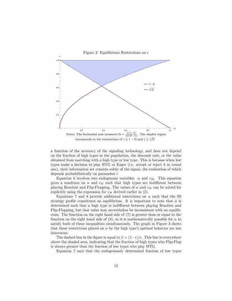
Figure 2: Equilibrium Restrictions on ε

1- W

W

0.2 0.4 0.6 0.8 1.0

W

0.2

0.4

0.6

0.8

1.0

Ε

Notes: The horizontal axis measures Ω =L(1−δ)λδ(H−L)

. The shaded region

corresponds to the intersection of ε ≥ 1− Ω and ε ≥√

Ω

a function of the accuracy of the signaling technology, and does not dependon the fraction of high types in the population, the discount rate, or the valueobtained from matching with a high type or low type. This is because when lowtypes make a decision to play HTG or Eager (i.e. accept or reject h in roundone), their information set consists solely of the signal, the realization of whichdepends probabilistically on parameter ε.

Equation 6 involves two endogenous variables: α and vH . This equationgives a condition on α and vH such that high types are indifferent betweenplaying Resolute and Flip-Flopping. The values of α and vH can be solved forexplicitly using the expression for vH derived earlier in (2).

Equations 7 and 8 provide additional restrictions on α such that the SSstrategy profile constitutes an equilibrium. It is important to note that α isdetermined such that a high type is indifferent between playing Resolute andFlip-Flopping, but that value may nevertheless be inconsistent with an equilib-rium. The function on the right hand side of (7) is greater than or equal to thefunction on the right hand side of (8), so it is mathematically possible for α tosatisfy both of these inequalities simultaneously. The graph in Figure 3 showsthat these restrictions placed on α by the high type’s optimal behavior are notinnocuous.

The dashed line in the figure is equal to β = (1−ε)/ε. This line is everywhereabove the shaded area, indicating that the fraction of high types who Flip-Flopis always greater than the fraction of low types who play HTG.

Equation 7 says that the endogenously determined fraction of low types

12

Figure 3: Equilibrium Restrictions on α

gHΕLhHΕLΒHΕL

0.6 0.7 0.8 0.9 1.0

Ε

0.2

0.4

0.6

0.8

1.0

gHΕL, hHΕL, ΒHΕL

playing HTG must be sufficiently low. When the fraction of low types playingHTG becomes too large, high types prefer to accept low signals (rather thanreject, as is called for in the SS equilibrium) because the costs of doing so aresufficiently low. That is, when α is large enough, accepting low signals in roundone becomes optimal not because it is more likely that the low signal came froma high type, but rather because the probability of actually forming a match witha low type is sufficiently low.

Equation 8 says that the endogenously determined fraction of low typesplaying HTG must be also be sufficiently high. If α is too low, then high typeswill not find it optimal to accept high-signals in round one. To understand whythis condition must be met, consider the extreme case where α = 0. Since a lowtype woman always accepts in round one in this case, high type men can ensurethat they never match with low type women by rejecting in round one. As thesignaling technology becomes more accurate (i.e. ε increases towards one), thislower bound on α falls towards 0.

6 Comparative statics

I now present results describing how equilibrium behavior and values dependon the parameters of the model. Ultimately, I am most interested in how play-ing HTG affects the set of matches which occur in equilibrium. Towards thatend, Proposition 2 below shows how the equilibrium strategies depend on theparameters of the model. This result will be especially useful in Section 7 whenanalyzing equilibrium mating.

13

Proposition 2. The equilibrium fraction of low types playing HTG

• decreases in the accuracy of the signaling technology, the discount rate,and the added benefit of mating with a high type;

• increases in the baseline value of mating relative to remaining single, and;

• can increase or decrease in the fraction of high types in the population.

The equilibrium fraction of high types Flip-Flopping is decreasing in the accuracyof the signaling technology and does not depend on the other parameters of themodel.

Proof. Please see Appendix A.2.

In addition to studying how equilibrium behavior depends on the model’sparameters, one might also be interested in the agents’ welfare in equilibrium.Proposition 3 details how low- and high types’ equilibrium values depend onthe parameters.

Proposition 3. The low type’s value

• increases in the discount rate, the baseline value of mating relative toremaining single, and the added benefit of mating with a high type;

• decreases in the accuracy of the signaling technology, and;

• can increase or decrease in the fraction of high types in the population.

The high type’s value increases in the fraction of high types in the population,the discount rate, the baseline value of mating relative to remaining single, andthe added benefit of mating with a high type.

Proof. Please see Appendix A.2.

Section 8 develops a numerical example of an environment in which the SSstrategy profile is an equilibrium. The example helps to illustrate the magnitudeof the comparative statics results. In the remainder of this section I will discussthe intuition behind some of these results.

Signal Accuracy: Consider an increase in the accuracy of the signaling tech-nology. Practically, such a change could occur when an institution or technologyevolves to allow agents better signals of their match-partners’ true underlyingtype. As examples, the advent and increased usage of social networking websitessuch as Facebook and LinkedIn make it easier for agents to learn more abouttheir potential match partners’ interests, abilities, and skills. Proposition 2 saysthat such changes lead to less within-match strategic behavior.

As the signaling technology becomes more informative, high types Flip-Flopless frequently. If this was not true, low types would have a strict incentive toplay HTG after observing a high signal because, the more accurate the signal,the more likely their partner is a high type who received a low signal.

14

Recall that the fraction of low types playing HTG is determined such thatjilted high types are indifferent between accepting and rejecting in round twoa low signal who rejected them in round one. As the accuracy of the signalingtechnology increases, holding all other variables constant, the probability thatone’s match-partner is a high type given the relationship history ` ∩ (R,R)decreases, and so high types are less inclined to accept. In order to keep hightypes indifferent between accepting and rejecting in this case, fewer low typesplay HTG.

As the accuracy of the signaling technology increases, the equilibrium valueto a low type falls because the likelihood of sending a low signal increases,low types play HTG less often, and they therefore match with high types lessfrequently.

The Baseline Value of Mating: In order to differentiate between the baselinevalue of mating relative to remaining single and the added benefit of mating witha high type, write H = L+G. Then increasing L makes mating with any partnermore attractive, while increasing G raises the benefit to mating specifically witha high type. As the baseline value of mating increases, the relative benefit toa high type with history ` ∩ (R,R) of waiting for a more promising partnerdecreases. In equilibrium, low types respond by playing HTG more often inorder to keep the high types in this situation indifferent between Flip-Floppingand playing Resolute.

The Added Benefit of Mating with a High type: If the value of mating with ahigh type increases but the fraction of low types playing HTG remains constant,high types in a relationship with history `∩(R,R) have a strict incentive to holdout and wait for a more promising partner next period. Therefore, low typesrespond by playing HTG less often in order to preserve high types’ indifference.

This result may be surprising in that one may initially think that as theadded benefit of mating with a high type increases, low types face greater in-centives to play HTG in order to increase their chances of marrying one of thesemore valuable partners. Absent from this sort of reasoning, however, are themoderating forces of equilibrium behavior. If low types played HTG more oftenas G increased, high types would stop Flip-Flopping and would instead playResolute. That is, high types would no longer give second chances to matchpartners who sent low signals and rejected, thereby removing any incentive toplay HTG at all.

Discounting: The fraction of low types playing HTG decreases in the dis-count rate. As the discount rate increases, men in relationships with history`∩ (R,R) are more willing to wait until next period in hopes of landing a morepromising match partner. In equilibrium, women must respond by playing HTGless often in order to keep these high type men indifferent between acceptingand rejecting.

High types’ equilibrium value increases in the discount rate because not onlydoes the value of a marriage with either type increase in the discount rate, buthigh types are more likely to mate with a fellow high type because the fractionof low types playing HTG decreases in the discount rate. To see that the lowtype’s value also increases in the discount rate, consider the Eager low type.

15

Increasing the discount rate does not affect the partners the Eager low typemarries, but it does increase the value of a marriage and decrease the cost ofwaiting until the next period. An increase in δ then raises the Eager low type’svalue, and since low types must be indifferent between playing HTG and Eager,the same holds for HTG low types.

Population Composition: The low type’s equilibrium value can increase ordecrease in the fraction of high types in the population. To see how the lowtype’s value could decrease in λ, recall that low types always mate with other lowtypes. When the proportion of high types increases, even though the expectedpayoff conditional on a match occurring increases, low types are less likely tomate because their match partners are more likely to be a discriminating hightype. This effect is most pronounced when agents are impatient (i.e. δ is small).

The high type’s equilibrium value always increases in λ. This is true regard-less of whether the fraction of low types playing HTG increases or decreasesbecause increasing λ increases the chances that a high type matches with an-other high type.

The fraction of low types playing HTG can either increase or decrease asλ increases. Recall that α is determined so that high types are indifferentbetween accepting and rejecting when their relationship history is ` ∩ (R,R).As λ increases and the high type’s continuation value of δvH increases, α mayneed to increase or decrease to keep high types indifferent between acceptingand rejecting.

7 Mating

Since types are private information and signals are noisy, it is inevitable thathigh types mate with low types in equilibrium. As might be expected, this canoccur when agents send inaccurate signals and the low type is using the Eagerstrategy. But this type of mismatch can also occur when both agents sendaccurate signals and the low type is playing HTG and the high type Flip-Flops.

I therefore use a stochastic notion of assortative mating closely related tothat in Chade [2006] – mating is positively assortative if the expected type ofone’s partner increases in one own’s type.14 Proposition 4 below formalizes thisconcept.

Proposition 4. Mating in the SS equilibrium is positively assortative – theexpected type of mate for a high type is greater than the expected type of matefor a low type.

Proof. The Eager low type man marries a low type woman for sure and marriesa high type woman only if he sends a high signal. Write the low type man’sexpected type of mate as

xL =(1− λ)L+ λ(1− ε)H

(1− λ) + λ(1− ε)14This definition of PAM originates in Shimer and Smith [2000], footnote 8.

16

The Resolute high type man marries a low type woman in one of two ways –first, she plays Eager and he sees a high signal, and second, she plays hard toget, he sees a high-signal, and she sees a low signal. The only way a Resolutehigh type man marries a high type woman is if both send high-signals. Thehigh type man’s expected type of mate is

xH =(1− λ)(1− ε)(1− αε)L+ λε2H

(1− λ)(1− ε)(1− αε) + λε2

Both xL and xH are weighted averages of L and H. Then xH > xL becausexH places relatively less weight on L and relatively more weight on H than xL.This is because ε2 > 1− ε so long as ε > (

√5−1)/2, which Figure 2 shows holds

in any SS equilibrium. This proves that high types have higher expected typesof partners than low types, and mating is therefore positively assortative.

PAM obtains in the SS equilibrium despite the low type agents’ attemptsat strategic misrepresentation. It is worth noting, however, that mating is notstrictly assortative on signals – low type agents who receive high-signals matewith high type agents who receive low signals in equilibrium.

I next show that the strategic behavior studied in this paper improves sort-ing. Consider, as a benchmark, the NS strategy profile discussed in Section 4:low types always accept, and high types accept high signals in the first round,and reject otherwise. In the appendix, I show that this strategy profile, alongwith beliefs derived using Bayes’ rule, can constitute a PBE.15 Moreover, theappendix shows that the SS and NS equilibria both exist over a range of param-eter values. Here in the text, I will focus on the efficiency gain from strategicbehavior.

Denote the present discounted match value created each period in the SSand NS equilibria as V SS and V NS , respectively. Proposition 5 shows thatthe strategic behavior in the SS equilibrium leads to more marriage value beingcreated than in the NS equilibrium. The proof shows that this increase in sortingis due to high types Flip-Flopping, and happens despite low types playing HTG.

Proposition 5. The steady state value of marriages created is always greaterin the SS equilibrium than in the NS equilibrium.

Proof. SS: Low types always marry other low types. Eager low types only marryhigh types if the Eager low type sends a high signal. HTG low types marry hightypes in two ways: first if both send inaccurate signals, and second if both sendaccurate signals and the high type Flip-Flops. High types marry other hightypes in two ways: first if both send the “correct” signals, and second if bothsend the “wrong” signals and both Flip-Flop. Since the probability high types

15The high types’ rejection in the second round after being rejected themselves is a weakbest response. While the NS strategy profile can be part of a PBE, it would not survive a“trembling hand” refinement.

17

Flip-Flop is β = (1− ε)/ε, this gives

V SS = 2(1− λ)2L2

1− δ+ 4(1− λ)λ

[(1− α)(1− ε) + α

((1− ε)2 + ε2

1− εε

)]LH

1− δ

+ 2λ2

(ε2 + (1− ε)2

(1− εε

)2)

H2

1− δ

NS: Low types always marry other low types. Low types and high types marryonly if the low type sends the high signal. High types marry if both send high-signals. This gives

V NS = 2(1− λ)2L2

1− δ+ 4λ(1− λ)(1− ε) LH

1− δ+ 2λ2ε2

H2

1− δ

To see that V SS > V NS , note that the term in square brackets in V SS simplifiesto 1− ε. Then

V SS − V NS = 2λ2(1− ε)4

ε2H2

1− δ> 0

Proposition 5 shows that the sorting gains in the SS equilibrium come fromthe high types Flip-Flopping. Low types attempt to increase mismatch usingthe HTG strategy, but this is ineffective in equilibrium. The probability a lowtype and high type marry is the same in each equilibrium, but the probabilitytwo high types marry is greater by the term (1 − ε)4/ε2 in the SS equilibriumbecause high types can marry even if both initially send low signals.

To be certain, the sorting gains are relatively modest. Figure 4 plots (1 −ε)4/ε2, which is the probability two Flip-Flopping high types send the low sig-nals. This figure shows that the probability that a matched pair of high typeagents will both play Flip-Flop and both send low- signals is relatively low –not much greater than 0.05, and likely much less over the relevant range ofε > 0.618. The increase in efficiency due to strategic behavior increases in thepayoff to marrying a high type and the degree of complementarity in maritalproduction.

8 Numerical example

In order to illustrate the existence and to give a sense of the magnitude of someof the qualitative results on behavior, mating, and welfare, this section providesa numerical example of the model. Fix the parameters of the model at ε = 0.75,δ = 0.8, L = 1, H = 3, and λ = 0.4. Then solving the system of equationsgiven by (2) and (6) gives α = 0.126 and vH = 24.9. Low types prefer willaccept a known low type because vL = 5.92, and so L2/(1 − δ) > δvL. Hightypes will not accept a known low type because δv2 > HL/(1− δ). High types

18

Figure 4: Limits to sorting gains of strategic behavior

0.6 0.7 0.8 0.9 1.0

Ε

0.05

0.10

0.15

H1 - ΕL4 Ε2

Notes: The horizontal axis measures ε. The vertical axis measures (1− ε)4/ε2, which is the

probability a matched pair of high types both Flip-Flop and send low signals. The dashed

vertical line occurs at ε = 0.618; there can be no SS equilibria with lower ε.

play Flip-Flop with probability 0.33. Lastly, α satisfies the innequalities in (7)and (8) because h(ε) = 0.018 and g(ε) = 0.133. So all of the conditions forthe Socially Strategic strategy profile to be an equilibrium are met. Table 1illustrates the effects of independently increasing each parameter by 1% on theagents’ behavior and values.

The Non-Strategic strategy profile is also an equilibrium for these parametervalues. The steady state value of marriages in the NS equilibrium is V NS = 15.3,while in the SS equilibrium it is V SS = 15.4.

Table 1: Comparative statics

1% increase in: ∆α ∆β ∆vH ∆vL

ε - 0.020 - 0.01 + 0.25 - 0.04

δ - 0.011 No change + 1.30 + 0.31

L + 0.003 No change + 0.04 + 0.08

H - 0.003 No change + 0.46 + 0.06

λ - 0.001 No change + 0.12 + 0.05Notes: Any?

19

9 Conclusion

This paper shows that, in addition to productive complementarities, the abilityto transfer utility between partners, and the existence of private informationover types, within-match strategic interaction matters in determining the set ofequilibrium marriages. Perhaps contrary to intuition, this within-match strate-gic behavior actually improves the efficiency of sorting.

I established the existence of a Socially Strategic equilibrium in the marriagemarket in which low type agents play hard to get in order to appear moredesirable to their partners. Using this strategy is not without costs, however,as marriages with some initially willing high types are derailed. In equilibrium,high type agents Flip-Flop with positive probability and accept in round twomarriages they initially found undesirable. I showed that mating in the SociallyStrategic equilibrium is stochastically positively assortative in that the expectedmate of a high type is better than the expected mate of a low type.

Moreover, the strategic behavior in the Socially Strategic equilibrium in-creases the sorting of mates relative to the Non-Strategic equilibrium. Whilelow types’ goal of playing hard to get is to increase mismatch, it is ineffectivein equilibrium. The increase in sorting efficiency is due entirely to the Flip-Flopping behavior of high types.

References

A. Anderson and L. Smith. Dynamic matching and evolving reputations. Reviewof Economic Studies, 77:3 – 29, 2010.

G. Becker. A theory of marriage: Part i. Journal of Political Economy, 81(4):813–846, 1973.

R. Bellman and D. Blackwell. Some two-person games involving bluffing. Pro-ceedings of the National Academy of Sciences of the United States of America,35:600 – 605, 1949.

H. Chade. Matching with noise and the acceptance curse. Journal of EconomicTheory, 129:81–113, 2006.

P. A. Coles and R. Shorrer. Optimal truncation in matching markets. Mimeo,2013.

M. E. Consuegra, R. Kumar, and G. Narasimhan. Comment on “On the unique-ness of stable marriage matchings”. Economics Letters, 121(3):468, 2013.

E. Damiano, L. Hao, and W. Suen. Unravelling of dynamic sorting. Review ofEconomic Studies, 72:1057–1076, 2005.

A. M. Franco, M. Mitchell, and G. Vereshchagina. Incentives and the structureof teams. Journal of Economic Theory, 146:2307–2332, 2011.

20

E. Hopkins. Job market signaling of relative position, or becker married tospence. Journal of the European Economic Association, 10(2):290–322, 2012.

R. Inderst. Matching markets with adverse selection. Journal of EconomicTheory, 121:145–166, 2005.

P. K. Jonason and N. P. Li. Playing hard-to-get: Manipulating one’s perceivedavailiability as a mate. European Journal of Personality, 27(5):458 – 469,2013.

J. M. McNamara and E. J. Collins. The job search problem as an employer-candidate game. Journal of Applied Probability, 27(4):815–827, 1990.

G. Moscarini. Job matching and the wage distribution. Econometrica, 73(2):481 – 516, 2005.

K. Serfes. Endogenous matching in a market with heterogeneous principals andagents. International Journal of Game Thoery, 36:587–619, 2008.

R. Shimer and L. Smith. Assortative matching and search. Econometrica, 68:343–369, 2000.

L. Smith. The marriage model with search frictions. Journal of Political Econ-omy, 114(6):1124 – 1144, 2006.

J. Von Neumann and O. Morgenstern. Theory of Games and Economic Behav-ior. Princeton University Press, Princeton, 1964.

D. J. Wright. The risk and incentives trade-off in the presence of heterogeneousmanagers. Journal of Economics, 83(3):209–223, 2004.

A Appendix

A.1 Proof of Proposition 1

Proof. The proof proceeds by deriving conditions on the model’s parameterssuch that agents optimally use the SS strategy profile (i.e. they have no prof-itable deviation). I begin in round two because some round one decisions willdepend on round two outcomes.

A.1.1 Low types in round two

The SS strategy profile requires both HTG and Eager low types to accept inround two, regardless of their relationhsip history. A condition sufficient toguarantee the optimality of this choice is that low types accept even if theyare sure their partner is a low type. This occurs if L2/(1 − δ) ≥ δvL. If thisinequality holds, then low types will also optimally accept when there is a chancetheir partner is a high type (which occurs when the low type is playing HTG,

21

observed a high signal and rejected in round one, and was rejected by theirpartner). Using (1), this inequality can be re-written to find that low typesprefer to accept known low types so long as ε ≥ 1− (1− δ)L/λδ(H − L). Thisinequality can hold for ε ∈ (1/2, 1) so long as λ, δ, and H are small enough andε and L are large enough.

A.1.2 High types in round two

Suppose the relationship history is ` ∩ (R,R) – the high type agent observeda low signal in round one, rejected a match, and was himself rejected. The SSstrategy profile calls for Flip-Floppers to accept in round two, but for thoseplaying Resolute to reject. High types must therefore be indifferent betweenannouncing A or R in this situation. Setting the expected value of A equal tothe expected value of R gives:

a2(`,H, (R,R))γ2(`,H, (R,R)) + (1− a2(`,H, (R,R)))δvH = δvH

⇔ γ2(`,H, (R,R)) = δvH

This equality can be simplified using the expressions in Table 2 as

(1− λ)ε2α LH1−δ + λ(1− ε)2β H2

1−δ(1− λ)ε2α+ λ(1− ε)2β

= δvH ⇒

αδvH − LH

1−δH2

1−δ − δvH= β

λ

1− λ

(1− εε

)2

(9)

When the above expression holds, high types are indifferent between playingResolute and Flip-Flopping, as they must be in order for β ∈ (0, 1).

In all other possible second round situations, the SS strategy profile callsfor high types to reject. In these situations, the high type does not know herpartner’s type, but she does know that only a low type agent would accept inthese situations in the second round. The expected match value, conditionalon a match occurring, is then LH/(1− δ). The high type agent then optimallyfollows the SS strategy profile by rejecting if the continuation value of δvH isgreater than the expected value of accepting, or:

δvH ≥ a2(θ,H, (Si, Sj))LH

1− δ+ (1− a2(θ,H, (Si, Sj)))δvH

⇒ δvH ≥LH

1− δ

After substituting in for vH using (2), simple algebra shows that the above holdswhen ε ≥

√(1− δ)L/λδ(H − L). So long as δ, λ, ε, and H are sufficiently large

and L is sufficiently small, high types prefer to reject and re-enter the pool ofthe unmatched than to accept and marry an agent who for sure a low type.

22

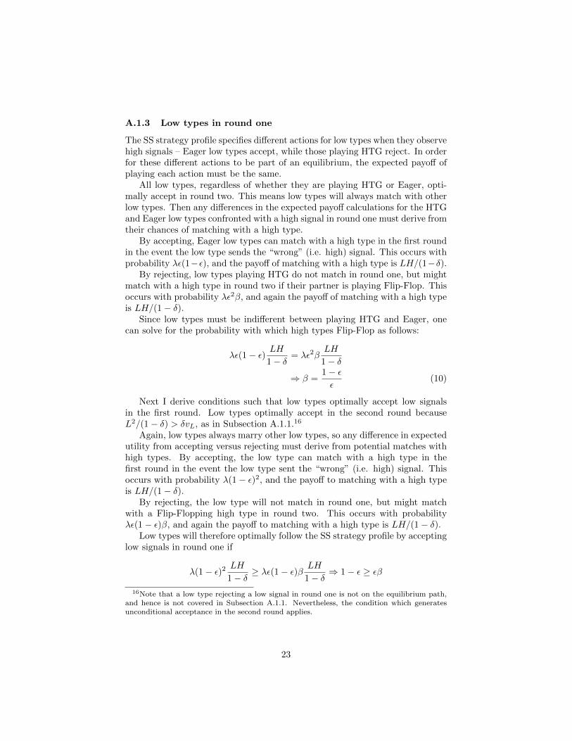
A.1.3 Low types in round one

The SS strategy profile specifies different actions for low types when they observehigh signals – Eager low types accept, while those playing HTG reject. In orderfor these different actions to be part of an equilibrium, the expected payoff ofplaying each action must be the same.

All low types, regardless of whether they are playing HTG or Eager, opti-mally accept in round two. This means low types will always match with otherlow types. Then any differences in the expected payoff calculations for the HTGand Eager low types confronted with a high signal in round one must derive fromtheir chances of matching with a high type.

By accepting, Eager low types can match with a high type in the first roundin the event the low type sends the “wrong” (i.e. high) signal. This occurs withprobability λε(1−ε), and the payoff of matching with a high type is LH/(1−δ).

By rejecting, low types playing HTG do not match in round one, but mightmatch with a high type in round two if their partner is playing Flip-Flop. Thisoccurs with probability λε2β, and again the payoff of matching with a high typeis LH/(1− δ).

Since low types must be indifferent between playing HTG and Eager, onecan solve for the probability with which high types Flip-Flop as follows:

λε(1− ε) LH1− δ

= λε2βLH

1− δ

⇒ β =1− εε

(10)

Next I derive conditions such that low types optimally accept low signalsin the first round. Low types optimally accept in the second round becauseL2/(1− δ) > δvL, as in Subsection A.1.1.16

Again, low types always marry other low types, so any difference in expectedutility from accepting versus rejecting must derive from potential matches withhigh types. By accepting, the low type can match with a high type in thefirst round in the event the low type sent the “wrong” (i.e. high) signal. Thisoccurs with probability λ(1− ε)2, and the payoff to matching with a high typeis LH/(1− δ).

By rejecting, the low type will not match in round one, but might matchwith a Flip-Flopping high type in round two. This occurs with probabilityλε(1− ε)β, and again the payoff to matching with a high type is LH/(1− δ).

Low types will therefore optimally follow the SS strategy profile by acceptinglow signals in round one if

λ(1− ε)2 LH1− δ

≥ λε(1− ε)β LH

1− δ⇒ 1− ε ≥ εβ

16Note that a low type rejecting a low signal in round one is not on the equilibrium path,and hence is not covered in Subsection A.1.1. Nevertheless, the condition which generatesunconditional acceptance in the second round applies.

23

But since β = (1 − ε)/ε in order for low types to be indifferent between play-ing HTG and Eager, the above expression holds with equality and low types(weakly) prefer to accept high-signals in round one.

A.1.4 High types in round one

Both strategies of the high type man call for the same action conditional on thewoman’s signal. Suppose initially the man observes signal ` in round one. I nowverify that it is indeed optimal for the man to reject as is called for by the SSstrategy profile.

If a high type man rejects a low signal in round one, he proceeds to the secondround for sure. Resolute high types then reject for sure, guaranteeing themselvesa continuation value of δvH . Of course, high types must be indifferent betweenplaying Resolute and Flip-Flopping, and so the Flip-Flopping high type mustreceive an expected payoff of δvH as well.

If a high type man deviates from the proposed equilibrium strategy andaccepts a low signal in round one, the probability he would consummate amarriage and the expected utility conditional on mutual acceptance is

a(`,H) =(1− λ)ε(1− αε) + λ(1− ε)ε

(1− λ)ε+ λ(1− ε)

γ(`,H) =(1− λ)ε(1− αε) LH1−δ + λ(1− ε)ε H

2

1−δ(1− λ)ε(1− αε) + λ(1− ε)ε

If a match does not occur in round one, however, it will not happen in roundtwo. This is because only low types playing HTG will accept in the second rounda partner who accepted in the first round, and high types prefer to re-enter thepool of the unmatched to marrying a low type.

The high type man then finds it optimal to play by the proposed equilibriumstrategy and to reject low signals if

δvH ≥ a(`,H)γ(`,H) + (1− a(`,H))δvH ⇔ δvH ≥ γ(`,H)

Substituting in for γ(`,H) and some minor manipulations allow the above con-dition to be re-written as

δvH − LH1−δ

H2

1−δ − δvH≥ λ

1− λ1− ε

1− αε

Substituting in from (9), the condition guaranteeing high types are indifferentbetween Flip-Flopping and playing Resolute, and the formula for β given in(10), followed by some simple manipulations gives

α ≤ (1− ε)2

ε3 + ε(1− ε)2≡ g(ε) (11)

So long as α satisfies the above condition, high types find it optimal to rejectlow signals in round one.

24

Next, suppose the high type man observes h in round one. The proposedequilibrium strategy calls for him to accept. The probability a match is consum-mated if he accepts and the expected payoff conditional on a match occurringare

a(h,H) =(1− λ)(1− ε)(1− αε) + λε2

(1− λ)(1− ε) + λε

γ(h,H) =(1− λ)(1− ε)(1− αε) LH1−δ + λε2 H

2

1−δ(1− λ)(1− ε)(1− αε) + λε2

Then a high type man’s expected utility of following the equilibrium strategyin round one when seeing h is

v(h,H|si = A) =(1− λ)(1− ε)(1− αε) LH1−δ + λε2 H

2

1−δ(1− λ)(1− ε) + λε

+(1− λ)(1− ε)εα+ λε(1− ε)

(1− λ)(1− ε) + λεδvH

(12)

If the high type man rejects, he proceeds to round two for sure. The prob-ability with which a high type man who observes h is accepted or rejected inround one is

Pr(Sj = R|h,H) =(1− λ)(1− ε)εα+ λε(1− ε)

(1− λ)(1− ε) + λε

Pr(Sj = A|h,H) =(1− λ)(1− ε)(1− α+ α(1− ε)) + λε2

(1− λ)(1− ε) + λε

According to the proposed equilibrium strategies, only low type women playingHTG and high type women reject in round one. The man will be accepted inround two if she is a low type playing HTG to whom he sent a high-signal ora Flip-Flopping high type to whom he sent a low signal. The probability he isaccepted and the expected payoff conditional on a match occurring are

a2(h,H, (R,R)) =(1− λ)(1− ε)εα+ λε(1− ε)β(1− λ)(1− ε)εα+ λε(1− ε)

γ2(h,H, (R,R)) =(1− λ)(1− ε)εα LH

1−δ + λε(1− ε)β H2

1−δ(1− λ)(1− ε)εα+ λε(1− ε)β

A high type man in a relationship with history h ∩ (R,R) will accept in roundtwo if γ2(h,H, (R,R)) ≥ δvH . Simple manipulations show that the high typeman accepts if

λε(1− ε)β(H2

1− δ− δvH

)≥ (1− λ)(1− ε)εα

(δvH −

LH

1− δ

)Note that the expression in Equation 9 implies that the above inequality alwaysholds, so that deviant high types in h ∩ (R,R) do in fact accept in round two.Expected utility in this case is

v2(h,H, (R,R)) =(1− λ)(1− ε)εα LH

1−δ + λε(1− ε)β H2

1−δ + λε(1− ε)(1− β)δvH

(1− λ)(1− ε)εα+ λε(1− ε)

25

I now compute the expected utility of a high type man in a relationship withthe history h ∩ (R,A). Since the man was accepted in round one, his partnercould be an Eager low type, a HTG low type to whom he sent `, or a high typeto whom he sent h. According to the SS strategy profile, only the low typewomen would ever accept in round two after they accepted in round two. Theprobability he is accepted is then

a2(h,H, (R,A)) =(1− λ)(1− ε)(1− α+ α(1− ε))

(1− λ)(1− ε)(1− α+ α(1− ε)) + λε2

The expected utility conditional on acceptance is γ2(h,H, (R,A)) = LH/1− δ.The high type man in a relationship with history h ∩ (R,A) therefore finds itoptimal to reject and get a payoff of δvH , which is greater than LH/(1− δ).

Then the expected utility of deviating in round one for the high type manwho observes h can be written

v(h,H|Si = R) =(1− λ)(1− ε)εα LH

1−δ + λε(1− ε)β H2

1−δ + λε(1− ε)(1− β)δvH

(1− λ)(1− ε) + λε

+(1− λ)(1− ε)(1− αε) + λε2

(1− λ)(1− ε) + λεδvH

(13)

In order for the high type man to play according to the SS strategy profile,the difference between (12) and (13) must be positive. The denominator of thisexpression is always positive, so the sign is determined by the numerator. Easymanipulations allow the numerator of this difference to be written as

v(h,H|Si = A)−v(h,H|Si = R) =

(1− λ)(1− ε)(1− αε)(LH

1− δ− δvH

)+ λε2

(H2

1− δ− δvH

)+ (1− λ)(1− ε)αε

(δvH −

LH

1− δ

)+ λ(1− ε)εβ

(δvH −

H2

1− δ

)Combining terms gives

v(h,H|Si = A)−v(h,H|Si = R) =

(1− λ)(1− ε)(2αε− 1)

(δvH −

LH

1− δ

)+ λε(ε− β(1− ε)

(H2

1− δ− δvH

)Simple manipulations show that, since α ≤ g(ε) implies 1− 2αε > 0, the aboveis positive whenever

λε(ε− β(1− ε))(1− λ)(1− ε)(1− 2αε)

≥δvH − LH

1−δH2

1−δ − δvH

26

Substituting in the value of β from (10) gives

λ(2ε− 1)

(1− λ)(1− ε)(1− 2αε)≥δvH − LH

1−δH2

1−δ − δvH

The equality in (9), the equation which specifies the value of α which makeshigh types indifferent between playing Resolute and Flip-Flopping, can be sub-stituted into the RHS of the above expression to get

λ(2ε− 1)

(1− λ)(1− ε)(1− 2αε)≥ λ(1− ε)2β

(1− λ)ε2α

The λ and 1−λ terms can be canceled. Again, since α < g(ε) implies 1−2αε > 0,cross multiplication gives

α(2ε− 1)ε2 ≥ (1− ε)3(1− 2αε)β

Substituting in β = (1−ε)/ε and rearranging to get α on the LHS and a functionof ε on the RHS gives

α ≥ (1− ε)4

(2ε− 1)ε3 + 2ε(1− ε)4≡ h(ε) (14)

If the above inequality holds, high types find it optimal to play according to theSS strategy profile and accept high signals in round one.

A.2 Proof of Propositions 2 and 3

Since the techniques are similar, I combine the proofs to limit repetition. Thecomparative static results on strategies and values are proved using a combi-nation of the Implicit Function Theorem and explicit differentiation. To easenotation, let χxy = xy/(1 − δ) denote each agent’s present discounted valuewhen a woman of type x marries a man of type y. The two endogenous vari-ables are α, the fraction of low types playing HTG, and vH , the high type’sexpected value. To use the IFT, I define a two-dimensional system of equationsg(α, vH ; t) = 0 as

g1(α, vH ; t) : αδvH − χLHχHH − δvH

− λ

1− λ

(1− εε

)3

= 0 ;

g2(α, vH ; t) : vH − (1− λ)(((1− ε)2 + ε(1− ε)(1− α))χLH + (ε(1− ε)α+ ε)δvH

)− λ

((1− ε2)δvH + ε2χHH

)= 0 ,

(15)where t represents a generic parameter. Let a = (α, vH). Then the Jacobian ofg(a; t) is

dg(a; t)

da=

δvH−χLHχHH−δvH αδ χHH−χLH

(χHH−δvH)2

−ε(1− ε)(1− λ)(δvH − χLH) 1− δ[(1− λ)ε(1 + α− αε) + λ(1− ε2)]

27

This matrix is invertible because the determinant is strictly positive since allterms are positive except the lower-left, which is negative. I do not explicitlywrite the − [dg(a; t)/da]

−1matrix here because it is quite cumbersome, but

denote the terms in this matrix by

−[dg(a; t)

da

]−1

=

(Z11 Z12

Z21 Z22

),

where Z11, Z21, and Z22 are negative and Z12 is positive.

A.2.1 Signal accuracy (ε)

Straight-forward differentiation shows that β = (1− ε)/ε is decreasing in ε. Toshow dα/dε < 0 I solve for α explicitly using (2) and (9) to get

α =(1− ε)3λ((1− ε)(1− λ)δL− (1− δ(ε+ λ− λε))H)

ε(1− λ)(ε2(1− δ)L− (H − L)λδ(1− 2ε(1− ε)(2− ε(1− ε))))

It is straightforward to show that the numerator is decreasing in ε. The deriva-tive of the denominator with respect to ε is

−(1− λ)λδ(H − L)

[3ε2

L(1− δ)λδ(H − L)

− (1− 8ε+ 18ε2 − 16ε3 + 10ε4)

]To see that this term is positive, recall from Subsection A.1.2 that ε >

√L(1− δ)/λδ(H − L),

and so the term in square brackets is greater than −1 + 8ε− 18ε2 + 16ε3 − 7ε4,which is negative over the relevant range of ε. This implies that the denominatorof α is increasing in ε, and so overall α decreases in ε.

Differentiation of (1) with respect to ε immediately gives the result that v1decreases in ε.

A.2.2 Fraction of high types (λ)

To see that α can increase or decrease in λ, one can compute the derivative andevaluate it in the following situations. Fix δ = 0.85, L = 1, H = 2, and λ = 0.5.When ε = 0.85, dα/dλ < 0, but when ε = 0.90, dα/dλ > 0.

To see that vL can increase or decrease in λ, differentiate as follows:

d

dλ

[(1− λ) L2

1−δ + λ(1− ε) LH1−δ1− λεδ

]=

(1− ε) LH1−δ − (1− δε) L2

1−δ(1− λεδ)2

Intuitively, when δ is large this expression is positive, but when δ is small enough,it can be negative.

I use the IFT to show that dvH/dλ > 0. The vector of derivatives withrespect to λ is

dg(a;λ)

dλ=

−(1−ε)3ε3(1−λ)2

−A(χHH − χLH)−B(δvH − χLH)

28

where A = ε2 and B = 1−ε(1+α)−ε2(1−α). The top term is clearly negative.To sign the bottom term, there are two cases to consider:

Case 1: A > 0, B > 0; the expression is negative because χHH − χLH and δvH −χLH are positive.

Case 2: A > 0, B ≤ 0; the expression is negative because A+B = (1−ε)(1−αε) > 0implies |A| > |B|, and χHH > δvH implies χHH − χLH > δvH − χLH .

This shows that the bottom term of dgdλ is negative, and since Z21 and Z22 are

also negative, dvHdλ > 0.

A.2.3 Discount rate (δ)

To show dα/dδ < 0 I solve for α explicitly using (2) and (9) to get

α =(1− ε)3λ((1− ε)(1− λ)δL− (1− δ(ε+ λ− λε))H)

ε(1− λ)(ε2(1− δ)L− (H − L)λδ(1− 2ε(1− ε)(2− ε(1− ε))))

It is straightforward to show that the derivative with respect to δ is negative.That vL is increasing in δ is easy to see given (1). The terms in the numerator

increase in δ while the denominator decreases, and so the overall expression forthe low type’s value is increasing in δ.

That vH increases in δ can be seen by solving explicitly for vH using (2) and(9) to get

vH =(1− λ)ε2(1− ε)LH + λH2 [1− 2ε(1− ε)(2− ε(1− ε))]

(1− δ)(ε2 − δε3 + δ(2ε− 1)(−1 + λε(2− ε(1− ε))))

Differentiation with respect to δ and some simplifications show that dvH/dδ > 0.

A.2.4 Added value of marrying a high type (G)

Letting H = L + G, the fraction of low types playing HTG can be explicitlywritten as

α =(1− ε)3λ(G+ L(1− δ)−Gδε−Gδλ(1− ε))

ε(1− λ)(−ε2(1− δ)L+Gδλ(1− 2ε(1− ε)(2− ε(1− ε))))

Then the derivative in G is

dα

dG= −

L(1− δ)(1− ε)3λ[ε2(1− δε) + λδ(2ε− 1)(2ε− 1− ε2 + ε3)

]ε(1− λ) (−ε2(1− δ)L+Gδλ(1− 2ε(1− ε)(2− ε(1− ε))))2

Then the sign of the derivative is opposite of the sign of the bracketed term inthe numerator. To see that the bracketed term is positive, note that

ε2(1− δε) + λδ(2ε− 1)(2ε− 1− ε2 + ε3) >

ε2(1− δε) + λδ(2ε− 1)(−ε2 + ε3) =

ε2 [(1− δε)− λδ(2ε− 1)(1− ε)] > 0

29

The first inequality holds because ε > 1/2, and the second inequality holdsbecause 1− δε > 1− ε and λδ(2ε− 1) < 1. Then the sign of dα/dG is negative.

Straight-forward differentiation of (1) shows that

dvLdG

=λ(1− ε)

(1− δ)(1− λεδ)> 0

I use the IFT to show that dvH/dG > 0. It is easy to show that both termsin the dg(a;G)/dG matrix are negative. Since Z21 and Z22 are also negative,this implies dvH/dG > 0.

A.2.5 Baseline value of marrying (L)

Differentiating the explicit expression of α with respect to L gives

dα

dL=G(1− δ)(1− ε)3λ

[ε2(1− δε) + λδ(2ε− 1)(2ε− 1− ε2 + ε3)

]ε(1− λ) (−ε2(1− δ)L+Gδλ(1− 2ε(1− ε)(2− ε(1− ε))))2

The bracketed term is the same as in dα/dG, which was determined to bepositive in Section A.2.4. Since all other terms are also positive, dα/dL > 0.

Straightforward differentiation of (1) shows that

dvLdL

=1− ελ

(1− δ)(1− λεδ)> 0

I use the IFT to show that vH is increasing in L. It is easy to show thatboth terms in the dg(a;L)/dL vector are negative. Since Z21 and Z22 are alsonegative, this implies dvH/dL > 0.

A.3 The Non-Strategic strategy profile

In this subsection I prove that the Non-Strategic (NS) strategy profile can bepart of a PBE and prove that the order of the discount rates is as depictedin Figure 1. Under the NS strategy profile, low types always accept, and hightypes accept high-signals in round one and otherwise reject. All information setsare reached with positive probability on the equilibrium path, so beliefs can becomputed using Bayes’ rule. I will show there are constellations of parameterssuch that this strategy profile constitutes a PBE.

Low types: It is sufficient to show that low types prefer to follow the NSstrategy rather than rejecting low-signals in both rounds. If low types optimallyaccept low signals in the first round, then it is also optimal to accept high signals.Moreover, rejecting only in the first round rules out the possibility of marryinga high type. The probability of acceptance and the expected utility conditionalon acceptance are

a(`, L) =(1− λ)ε+ λ(1− ε)2

(1− λ)ε+ λ(1− ε); γ(`, L) =

(1− λ)ε L2

1−δ + λ(1− ε)2 LH1−δ(1− λ)ε+ λ(1− ε)2

30

The expected utility of playing according to the NS strategy profile and accept-ing is v(`, L|si = A) = a(`, L)γ(`, L) + (1 − a(`, L))vL, where vL is the sameas in (1). The expected utility of rejecting in both rounds is δvL. Low typesoptimally accept low signals if v(`, L|si = A) ≥ δvL. Simple algebra allows thisinequality to be re-written

δ ≤ (1− λ)εL+ λ(1− ε)2H(1− λ)(ε+ λ+ λε(2ε− 3))L+ λ(1− ε)(λ− ε(2λ− 1))H

≡ δNS

Subtracting the numerator from the denominator shows that δNS < 1.High types: It is sufficient to show that high types prefer to follow the NS

strategy rather than accepting low-signals in round one. If high types optimallyreject low signals in round one, then it is also optimal to reject in round two. Theprobability of acceptance and the expected utility conditional on acceptance are

a(`,H) =(1− λ)ε+ λ(1− ε)ε(1− λ)ε+ λ(1− ε)

; γ(`,H) =(1− λ)ε LH1−δ + λ(1− ε)ε H

2

1−δ(1− λ)ε+ λ(1− ε)ε

The expected utility of accepting a low signal is v(`,H|si = A) = a(`,H)γ(`,H)+(1− a(`,H))δvH , where

vH =(1− λ)(1− ε) LH1−δ + λε2 H

2

1−δ1− (1− λ)εδ − λ(1− ε2)δ

The expected utility of rejecting is δvH . High types optimally reject if δvH ≥v(`,H|si = A). Simple algebra allows this inequality to be re-written

δ ≥ L− λ(L− (1− ε)H)

L+ ελ(H − 2L)− (H − L)(2ε− 1)λ2≡ δNS

So long as δ ∈ (δNS , δNS), the NS strategy profile and beliefs derived usingBayes’ rule constitute a PBE.

But note this equilibrium involves a weakly dominated strategy – when twohigh types are in a relationship in which both saw low signals and both rejecteda marriage, they believe with probability equal to one that their match partneris a high type. Nevertheless, rejecting is a weak best response given that thepartner follows the equilibrium strategy and rejects. So while this strategyprofile is a PBE, it involves weakly dominated strategies and is not a TremblingHand Perfect equilibrium.

It is possible to order the discount rates for which the SS and NS strategyprofiles are PBE. Let δSS and δSS be the lowest and highest discount rate,respectively, such that a SS equilibrium exists.

Proposition 6. δNS < δSS < δSS < δNS

Proof. Note that δSS comes from L2/(1 − δ) ≥ δvL, which can be rearrangedto get

δ ≤ L

(1− λ(1− ε))L+ λ(1− ε)H≡ δSS

31

To see that δSS < δNS , write δNS = (AL+BH)/(CL+DH), where

A =(1− λ)ε

ε+ λ− λε(3− ε); B =

λ(1− ε)2

ε+ λ− λε(3− ε)

C =(1− λ)(ε+ λ+ λε(2ε− 3))

ε+ λ− λε(3− ε); D =

λ(1− ε)(λ− 2λε+ ε)

ε+ λ− λε(3− ε)

Rewrite δSS = L/[(1− E)L+ EH], where E = λ(1− ε).

AL+BH − L =λ(1− ε)2(H − L)

ε+ λ− λε(3− ε)≡ Z > 0

CL+DH − [(1− E)L+ EH] =λ2ε(1− ε)2(H − L)

ε+ λ− λε(3− ε)≡ λεZ > 0

Then

δNS − δSS =AL+BH

CL+DH− AL+BH − ZCL+DH − λεZ

= Z1

CL+DH

1

CL+DH − λεZ

((CL+DH)− λε(AL+BH)

)> 0 ,

where the last inequality holds because δNS < 1 and λε < 1.I next show that δSS > δNS . It is possible to solve explicityly for α, the

equilibrium fraction of low types playing HTG, while imposing δ = δNS . Then,subtracting the upper bound for α, g(ε) = (1 − ε)2/(ε3 + ε(1 − ε)2) from theresult gives

H(1− ε)4(2ε− 1)

ε(1− 2ε(1− ε))[(1− λ)(1− ε)L(1− 2ε(1− ε)) + λH(1− 2ε(1− ε)(2− ε(1− ε)))]This expression is positive for all ε ∈ (1/2, 1), which shows that optimal behaviorwith δ = δNS is not consistent with the SS equilibrium.

Since α is too large, and Proposition 2 shows that α is decreasing in δ, wemust have δSS > δNS .

A.4 Updating table

Table 2 below is included to assist the reader in performing second round infer-ence calculations. The first column lists the two different types, and the secondcolumn lists each type’s possible strategies. The third column lists all possi-ble histories in which a man could find himself in round two. The descriptionof the history involves signal θ and realized round one announcements (si, sj),where si is the man’s announcement and sj is the woman’s announcement. Acrossed-out history indicates it does not occur in equilibrium. The fourth col-umn of the table lists the action called for by the SS strategy profile. The fifthcolumn lists a2(θ, y, (si, sj)). These probabilities are computed by combiningthe Bayesian updating given the relationship history in the third column withthe SS strategy profile. Lastly, the sixth column lists the expected payoff ofaccepting conditional on a match occurring.

32

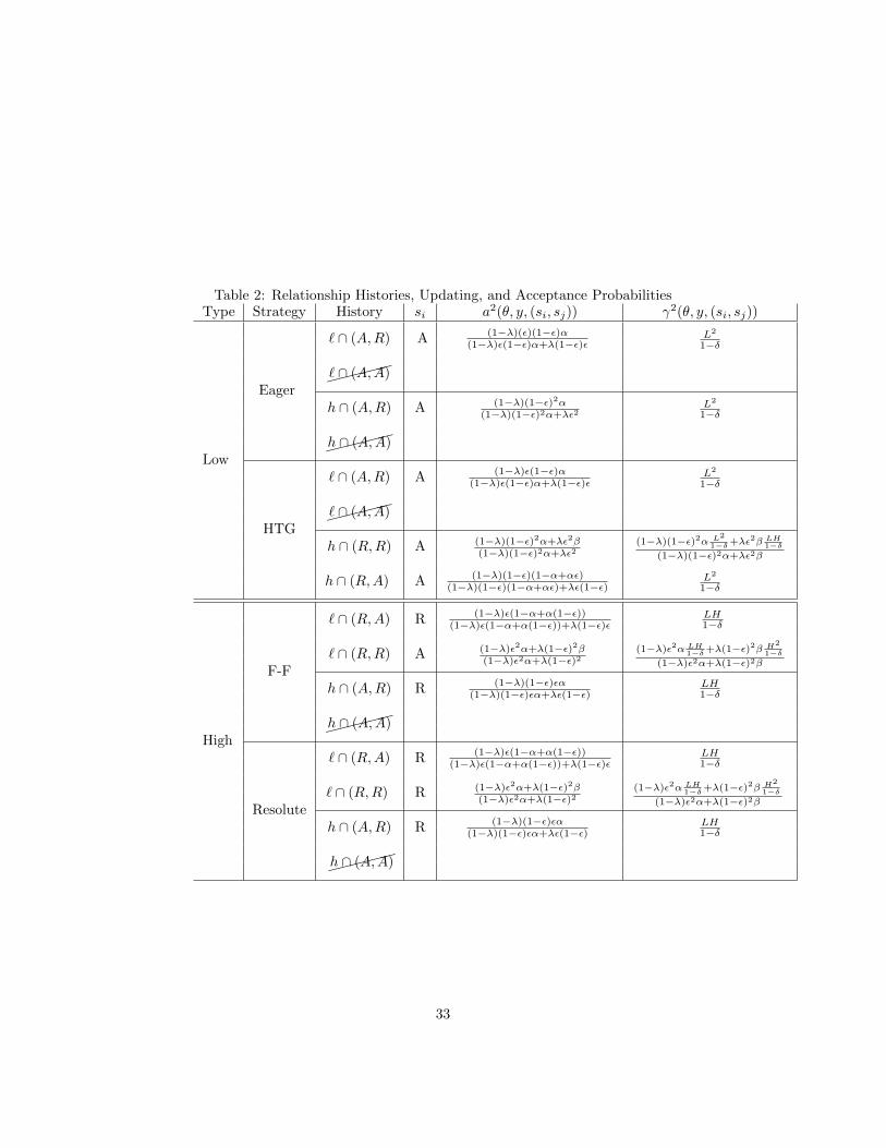
Table 2: Relationship Histories, Updating, and Acceptance ProbabilitiesType Strategy History si a2(θ, y, (si, sj)) γ2(θ, y, (si, sj))

Low

Eager

` ∩ (A,R) A (1−λ)(ε)(1−ε)α(1−λ)ε(1−ε)α+λ(1−ε)ε

L2

1−δ

` ∩ (A,A)

h ∩ (A,R) A (1−λ)(1−ε)2α(1−λ)(1−ε)2α+λε2

L2

1−δ

h ∩ (A,A)

HTG

` ∩ (A,R) A (1−λ)ε(1−ε)α(1−λ)ε(1−ε)α+λ(1−ε)ε

L2

1−δ

` ∩ (A,A)

h ∩ (R,R) A (1−λ)(1−ε)2α+λε2β(1−λ)(1−ε)2α+λε2

(1−λ)(1−ε)2α L2

1−δ+λε2β LH1−δ

(1−λ)(1−ε)2α+λε2β

h ∩ (R,A) A (1−λ)(1−ε)(1−α+αε)(1−λ)(1−ε)(1−α+αε)+λε(1−ε)

L2

1−δ

High

F-F

` ∩ (R,A) R (1−λ)ε(1−α+α(1−ε))(1−λ)ε(1−α+α(1−ε))+λ(1−ε)ε

LH1−δ

` ∩ (R,R) A (1−λ)ε2α+λ(1−ε)2β(1−λ)ε2α+λ(1−ε)2

(1−λ)ε2α LH1−δ+λ(1−ε)

2β H2

1−δ(1−λ)ε2α+λ(1−ε)2β

h ∩ (A,R) R (1−λ)(1−ε)εα(1−λ)(1−ε)εα+λε(1−ε)

LH1−δ

h ∩ (A,A)

Resolute

` ∩ (R,A) R (1−λ)ε(1−α+α(1−ε))(1−λ)ε(1−α+α(1−ε))+λ(1−ε)ε

LH1−δ

` ∩ (R,R) R (1−λ)ε2α+λ(1−ε)2β(1−λ)ε2α+λ(1−ε)2

(1−λ)ε2α LH1−δ+λ(1−ε)

2β H2

1−δ(1−λ)ε2α+λ(1−ε)2β

h ∩ (A,R) R (1−λ)(1−ε)εα(1−λ)(1−ε)εα+λε(1−ε)

LH1−δ

h ∩ (A,A)

33