Module 3

63

Plate Perforation Analysis

Type of Solver: ABAQUS CAE/Explicit

Dynamic Analysis – Plate Perforation from Projectile Impact

Introduction:

Perforation of metallic plates during projectile impact is a complex process,

commonly involving elastic and plastic deformation, strain and strain rate hardening

effects, thermal softening, crack formation, adiabatic shearing, plugging, petalling and

even shattering. These effects depend on the properties and geometries of projectile and

target and on the relative velocity of the colliding bodies. In this practical class, you will

model the perforation of a deformable metallic plate when struck by a rigid, spherical

projectile over a range of impact velocities. You will run analyses assuming both rate

dependent and rate-independent material behaviour, and compare your predictions.

Problem Description:

You have been asked by the Ministry of Defence to determine the ballistic limit

(minimum impact velocity required to fully perforate a target) of 0.4 mm thick steel plates,

impacted by spherical projectiles that are 8 mm in diameter. The projectiles have a mass

of 0.002 kg. The steel mechanical properties have been measured for you. The plastic

mechanical behaviour is well described by the Johnson and Cook phenomenological

plasticity model.

Module 3

64

Johnson-Cook Theory

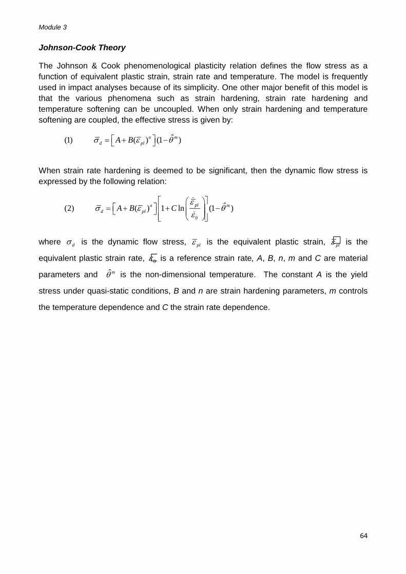
The Johnson & Cook phenomenological plasticity relation defines the flow stress as a function of equivalent plastic strain, strain rate and temperature. The model is frequently used in impact analyses because of its simplicity. One other major benefit of this model is that the various phenomena such as strain hardening, strain rate hardening and temperature softening can be uncoupled. When only strain hardening and temperature softening are coupled, the effective stress is given by:

When strain rate hardening is deemed to be significant, then the dynamic flow stress is expressed by the following relation:

0

ˆ(2) ( ) 1 ln (1 )pln md plA B C

εσ ε θ

ε

= + + −

where dσ is the dynamic flow stress, plε is the equivalent plastic strain, plε is the

equivalent plastic strain rate, 0ε is a reference strain rate, A, B, n, m and C are material

parameters and ˆmθ is the non-dimensional temperature. The constant A is the yield

stress under quasi-static conditions, B and n are strain hardening parameters, m controls

the temperature dependence and C the strain rate dependence.

ˆ(1) ( ) (1 )n md plA Bσ ε θ = + −

Module 3

65

(a) Build a 3-dimensional FE model. Since the plates are so thin, assume their

geometry can be represented by a shell with an 80 mm diameter. Assume also that the

projectile does not deform (either elastically or plastically). Beyond the elastic limit, the

strain hardening behaviour of the plate is best described using the Johnson and Cook

constitutive plasticity model (Eq.1) – recall that this equation neglects any strain rate

hardening contribution. Fracture in the plates will be modelled using a very simple critical

plastic strain fracture criterion. The Johnson and Cook material property data for Weldox

460E steel are given in Table I. Using this information, determine the ballistic limit of the

steel plates when struck normal to their plane, using a measured (quasi-static) uniaxial

plastic fracture strain of 0.33. Predict also the energy absorbed by the steel plates for 5

impact speeds between the ballistic limit and 600 m s-1, when struck normal to their plane.

(b) Strain rate hardening effects were neglected in (a). However, the steel plates are

known to exhibit rate-hardening behaviour. Fortunately, the Johnson and Cook plasticity

model can be modified to include the effects of strain rate hardening (Eq.2). Modify your

existing material model to include the Johnson and Cook strain rate hardening parameters

(Table I) and the strain rate-dependent fracture behaviour (Table II). Re-run your

simulations, and predict new ballistic limit and the absorbed energy as a function of the

impact speed once more. Compare these predictions with those from (a). Comment on the

significance of strain rate hardening in this particular steel alloy.

(c) (OPTIONAL) Determine the ballistic limit of the steel plates when impacted at 45°.

Use the fully coupled form of the Johnson and Cook equation.

Module 3

66

Material Property Data

Table III

Density Elastic Constants ρ E ν

kg m-3 GPa

7800 200 0.33

Table I Johnson and Cook Material Property Data

Ref.Strain

A B n m Tmelt Ttran C rate Mpa Mpa K K s-1

310 1000 0.65 1 1673 293 0.07 0.01

Table II Rate-dependent Fracture Data Strain Rate Stress Triaxiality Fracture Strain

s-1 0.01 0.33 0.33 0.1 0.33 0.32 1 0.33 0.31

10 0.33 0.30 100 0.33 0.29

1000 0.33 0.28 10000 0.33 0.27

Module 3

67

Solution (a):

• Start ABAQUS/CAE. At the Start Session dialogue box, click Create Model Database.

• From the main menu bar, select Model→Create. The Edit Model Attributes dialogue box

appears; name the model Plate Perforation

Under the Part module, we will construct the plate and projectile.

1. From the main menu bar, select Part→Create

2. The Create Part Dialogue box appears. Name the part Steel Plate and fill in the options as shown in Fig.A1. Click Continue to create the part.

3. From the main menu bar, select Add→Circle

(a) Select the co-ordinates (0, 0) for the centre of the circle in the prompt area. (b) Select the co-ordinates (0.04, 0) for the perimeter point

(c) Click and then Done in the prompt area.

4. You must now create two partitions. From the main menu bar

select Tools→Partition. The Create Partition dialogue box will open

(Fig.A2).

(a) Select Face as the Type and Sketch as the Method.

(b) Using the mouse cursor select the edge of the part.

(c) Using the Create Circle tool, create two circles; one with a

diameter of 70 mm and the other with a diameter of 10 mm

(d) Click and then Done in the prompt area.

5. Now create an Analytical Rigid spherical projectile with an 8 mm diameter (Fig.A3). Once

done, create a Reference Point at the centre. (Tools→Reference Point).

6. Create a set at the Reference Point and call it Projectile Set.

A. MODULE→PART

Fig.A1

Fig.A2

Fig.A3

Reference Point

Module 3

68

In this module (property), you will define the plate material properties. The strain hardening behaviour will be described using the Johnson and Cook plasticity relation. Fracture will be modelled by defining a critical plastic strain.

1. From the toolbox, select the Create Material tool. The Edit Material dialogue box will open.

(a) Name the material Weldox 460E.

(b) Define the density and elastic constants (Table III).

(c) Select Mechanical→Plasticity→Plastic as shown in Fig.B1.

(d) Under Hardening, select Johnson-Cook (Fig.B2). Fill in the data according to Table I.

(e) To define the critical plastic strain at fracture, select Mechanical→Damage for Ductile Metals→Ductile Damage (Fig.B3). The quasi-static fracture strain is 0.33. The stress triaxiality is 0.33 and the reference strain rate is 0.01.

(f) In the Suboptions drop-down menu, select Damage Evolution (Fig.B4). Choose a Displacement at Failure value of 0.0001 (Fig.B5). Click OK. Click OK again.

B. MODULE→PROPERTY

Fig.B1 Fig.B2 Fig.B3

Fig.B4

Fig.B5

Module 3

69

2. From the main menu bar select Section→Create. The Create Section dialogue box will open.

Fill in the Create Section dialogue box as shown in Fig.B6 and click Continue.

3. The Edit Section dialogue box will appear (Fig.B7). You must

now define the thickness of the plate (0.4 mm). Click OK.

4. From the main menu bar select Assign→Section. Using the

mouse cursor, click and drag across the plate and click Done in

the prompt area. Click OK in the Edit Section Assignment dialogue box. Click Done in the prompt area.

**Whilst in the Property module, you must also specify the projectile mass!!

5. From the main menu bar, select Special→Inertia→Create. The Create Inertia dialogue box will open. Name the mass condition Projectile Mass and select Point Mass as the Type. Click Continue. Select the Reference Point you created in the Part module as the point to which you wish to assign mass. Click Done in the prompt area and the Edit Inertia dialogue box will open. Select a mass of 0.002 kg and click OK.

1. From the main menu bar select Instance→Create. The Create Instance dialogue box will open. Select both of the parts and choose Independent as the Instance Type. Click OK.

2. Translate the projectile in the Positive Z direction by 6 mm (Instance→Translate). Click OK in the prompt area.

C. MODULE→ASSEMBLY

Fig.B6

Fig.B7

Module 3

70

1. From the main menu bar, select Step→Create. The Create Step dialogue box will appear Name the step Impact Step.

2. Select General from the Procedure Type options.

3. Select Dynamic, Explicit from the list of analysis types. Click Continue. The Edit Step dialogue box will open. Choose a time period of 0.0002 s (200 µs). Toggle on NLGEOM. Click OK.

4. Failed elements will need to be removed from the mesh in order to monitor crack propagation in your analyses. In the Field Output Requests, toggle on Status, which can be found under the State/Field/User/Time options.

5. To monitor the projectile velocity, create a new History Output Request called Projectile Velocity. Choose Projectile Set for the Domain and select V3, from the V options underneath the Displacement/Velocity/Acceleration list.

1. From the main menu bar select Interaction→Create. The Create Interaction dialogue box will open.

(a) Name the interaction Projectile Plate Contact.

(b) Choose Surface-to-Surface for the Types for Selected Step.

(c) Click Continue.

2. You will be prompted to select the first (Master) surface. Using the mouse cursor, select the surface of the analytical rigid projectile and click Done in the prompt area.

3. When prompted, choose Brown in the prompt area, which represents the outer surface of the projectile.

4. You now need to define the second (Slave) surface involved in the contact. Select Surface from the prompt area. Using the mouse cursor, select the inner, partitioned region of the plate (Fig.E1). Click Done in the prompt area. Select Brown when prompted to choose a side for the shell surface.

5. The Edit Interaction dialogue box will open (Fig.E2). From the Discretisation Method select Surface to Surface.

6. Click the Create tab next to Contact Interaction Property. The Create Interaction Property dialogue box will open.

7. Name it Contact Interaction and select Contact as the Type. Click Continue and the Edit Contact Property box will open. Select Mechanical→Normal, and accept the default options by clicking OK. Click OK again.

D. MODULE→STEP

E. MODULE→INTERACTION

Fig.E1 Fig.E2

Module 3

71

1. From the main menu bar select BC→Create. The Create Boundary Condition dialogue box will open (Fig.F1)

(a) Name the boundary condition Clamp.

(b) Choose Mechanical for the category.

(c) Choose Symmetry/Antisymmetry/Encastre for the Types for Selected Step.

(d) Click Continue.

(e) You must now select the region for the Clamp boundary condition as shown in Fig.F2.

2. Click Done in the prompt area. The Edit Boundary Condition dialogue box will open. Select Encastre and click OK.

3. Create a further boundary condition that will allow the projectile to move in the Z-direction (axis-3) only. Assign this boundary condition to the projectile Reference Point that you created earlier.

4. To define the projectile velocity, from the main menu bar select Predefined Field→Create. Select the options shown in Fig.F3 for the Create Predefined Field dialogue box. Click Continue.

5. When prompted to select the region for the Predefined Field, select the projectile Reference Point once more. Click Done in the prompt area.

6. In the Edit Predefined Field dialogue box that appears, choose V1=V2=0 and V3=-150. Click OK when done.

F. MODULE→LOAD

Fig.F1 Fig.F2

Fig.F3

Module 3

72

1. From the main menu bar, select Mesh→Controls. Using the mouse cursor, click and drag across the plate (remove the projectile using the viewing options!).

(a) Select Quad as the Element Type.

(b) Select Free as the Technique.

(c) Select Medial Axis as the Algorithm type.

(d) Click OK.

2. Using the Seed options, seed all 3 edges with 50 seeds using the Seed Edge by Number option.

3. From the main menu bar select Mesh→Element Type. Click and drag the mouse cursor over the plate and click Done in the prompt area. The Element Type dialogue box will open. Select Explicit from the Element Library and Shell from the Element Family options. Choose Quad elements and click OK to choose the S4R element type. Click Done in the prompt area.

4. From the main menu bar select Mesh→Instance. Using the mouse cursor, select the plate and click Done in the prompt area

**There is no time during the session today to conduct a mesh sensitivity analysis. However, you should bear in mind that, for simulations of this type, the results can be very sensitive to your choice of mesh. Under normal circumstances, you MUST conduct a sensitivity analysis.

1. Create a job titled WeldoxBL and submit the job for analysis. The job should take approximately one to two minutes.

1. From the main menu bar select Results→Field Output. From the Field Output dialogue box select Mises Stress. Make a note of whether or not the plate has fully perforated (i.e. Fig.H1). If not, increase the impact velocity in the Load module. If it has, decrease the impact velocity in the Load module. Continue to do this until you converge upon the ballistic limit.

2. The projectile velocity data can be found from the History Output options accessible from the main menu bar. Using this information, calculate the absorbed energy (energy lost by the projectile) for impact velocities of 150, 200, 300, 400 500 and 600 m s-1.

G. MODULE→MESH

G. MODULE→JOB

H. MODULE→VISUALISATION

Module 3

73

Solution (b):

• Return to the Property module. Using the strain rate hardening and strain rate

fracture data from Table I and Table II, define strain rate-hardening behaviour in

your material model

1. From the main menu bar select Material→Edit→Weldox 460E.

(a) Select Mechanical→Plasticity→Plastic.

(b) Under the Suboptions tab select Rate Dependent.

(c) Under Hardening select Johnson-Cook and fill in the rate-hardening data from Table I

2. Select Ductile Damage from the Material Behaviours box. Fill in the rate-dependent fracture strain data as shown in Table II.

1. Determine the ballistic limit of the plate with these new material property characteristics by submitting the necessary jobs. *You may need to alter the step time for low impact velocities. Submit 5 further jobs at impact speeds between the ballistic limit and 600 m s-1.

1. View the Mises Stress contours by selecting Results→Field Output from the main menu bar. Calculate the absorbed energy by extracting the projectile velocity history.

A. MODULE→PROPERTY

Fig.H1

B. MODULE→JOB

C. MODULE→VISUALISATION

Module 3

74

1. Determine the ballistic limit of the plates when struck at an angle of 45°.

2. The effects of friction have not been considered in these analyses. Using the FE model, and assuming a friction co-efficient between the projectile and the plate of 0.18, determine whether or not there is a contribution to absorbed energy from friction. How much more significant is friction when the angle of incidence is 45° compared to when the plate is struck at normal incidence for an impact velocity of 300 m s-1. (*Hint; return to your contact interaction property and search under tangential behaviour.)

3. The strain and strain rate-dependent behaviour has been described using the Johnson-Cook constitutive relation. Is there an alternative way of defining this data in the material editor?

4. In the strain rate-dependent simulations, you defined rate-dependent fracture strains for strain rates as high as 10000 s-1. Is this strain rate-dependent fracture data sufficient to cover the range of strain rates that are generated at the highest impact velocities? (*Hint; you will need to edit the field output requests to include strain rates as output data.)

OPTIONAL QUESTIONS