planning of cascade hydropower stations with the
TRANSCRIPT
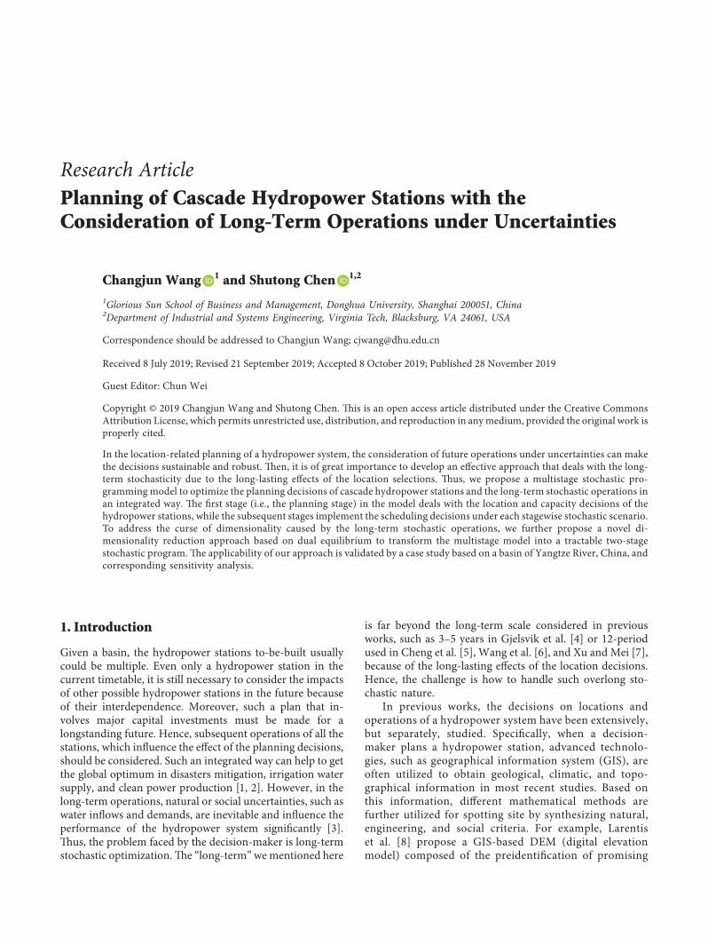
Research ArticlePlanning of Cascade Hydropower Stations with theConsideration of Long-Term Operations under Uncertainties
Changjun Wang 1 and Shutong Chen 12
1Glorious Sun School of Business and Management Donghua University Shanghai 200051 China2Department of Industrial and Systems Engineering Virginia Tech Blacksburg VA 24061 USA
Correspondence should be addressed to Changjun Wang cjwangdhueducn
Received 8 July 2019 Revised 21 September 2019 Accepted 8 October 2019 Published 28 November 2019
Guest Editor Chun Wei
Copyright copy 2019 Changjun Wang and Shutong Chen )is is an open access article distributed under the Creative CommonsAttribution License which permits unrestricted use distribution and reproduction in anymedium provided the original work isproperly cited
In the location-related planning of a hydropower system the consideration of future operations under uncertainties can makethe decisions sustainable and robust )en it is of great importance to develop an effective approach that deals with the long-term stochasticity due to the long-lasting effects of the location selections )us we propose a multistage stochastic pro-gramming model to optimize the planning decisions of cascade hydropower stations and the long-term stochastic operations inan integrated way )e first stage (ie the planning stage) in the model deals with the location and capacity decisions of thehydropower stations while the subsequent stages implement the scheduling decisions under each stagewise stochastic scenarioTo address the curse of dimensionality caused by the long-term stochastic operations we further propose a novel di-mensionality reduction approach based on dual equilibrium to transform the multistage model into a tractable two-stagestochastic program)e applicability of our approach is validated by a case study based on a basin of Yangtze River China andcorresponding sensitivity analysis
1 Introduction
Given a basin the hydropower stations to-be-built usuallycould be multiple Even only a hydropower station in thecurrent timetable it is still necessary to consider the impactsof other possible hydropower stations in the future becauseof their interdependence Moreover such a plan that in-volves major capital investments must be made for alongstanding future Hence subsequent operations of all thestations which influence the effect of the planning decisionsshould be considered Such an integrated way can help to getthe global optimum in disasters mitigation irrigation watersupply and clean power production [1 2] However in thelong-term operations natural or social uncertainties such aswater inflows and demands are inevitable and influence theperformance of the hydropower system significantly [3])us the problem faced by the decision-maker is long-termstochastic optimization)e ldquolong-termrdquo wementioned here
is far beyond the long-term scale considered in previousworks such as 3ndash5 years in Gjelsvik et al [4] or 12-periodused in Cheng et al [5] Wang et al [6] and Xu and Mei [7]because of the long-lasting effects of the location decisionsHence the challenge is how to handle such overlong sto-chastic nature
In previous works the decisions on locations andoperations of a hydropower system have been extensivelybut separately studied Specifically when a decision-maker plans a hydropower station advanced technolo-gies such as geographical information system (GIS) areoften utilized to obtain geological climatic and topo-graphical information in most recent studies Based onthis information different mathematical methods arefurther utilized for spotting site by synthesizing naturalengineering and social criteria For example Larentiset al [8] propose a GIS-based DEM (digital elevationmodel) composed of the preidentification of promising
sites and the multicriteria feasibility assessment of thefinal set in which energy technical and environmentalfactors are considered together Another GIS-based DEMis proposed by Kusre et al [9] which use a hydrologicmodel to assess water resource utilization under differentsite candidates Similar works can be referred to Serpoushet al [10] Zaidi and Khan [11] etc Besides the aboveassessment models the optimization technique becomesanother alternative in recent years For example Hosnarand Kovac-Kralj [12] identify the optimal installationlocations by maximizing an ecoprofit objective at tech-nological economic environmental and social con-straints To identify the appropriate hydropower damlocation Loannidou and OrsquoHanley [13] develop a mixed-integer linear programming model to optimize the hy-dropower potential with the consideration of river con-nectivity In these studies the future power generationand hydrologic dynamics are described by the empiricalformulas in the cumulative form )us time-varyingoperations under uncertainties are ignored in the settingof location-related planning
)e optimization of the multistage operational ac-tivities such as water storage supply and power gen-eration is an important issue which has drawn lots ofstudies Most of them focus on a given hydropowersystem involving a single hydropower plant (eg Vieiraet al [14]) or multistations For the multistation oper-ations in the deterministic setting two main stream ofapproaches have been applied At first to pursue theoptimality mathematical programming methods espe-cially dynamic programming (DP) are often used butalso suffer from the computational challenge due to thenumber of stages and stations )us Cheng et al [15]reduce the scale of the problem by limiting their work inthe ldquoshort-termrdquo horizon Li et al [16] consider a de-composition-coordination mechanism to reduce di-mensionality Li et al [17] and Cheng et al [5] propose toparallelize the DP algorithm to reduce the computationtime )e former uses the distributed memory archi-tecture and the message passing interface protocol whilethe latter considers the ForkJoin parallel framework in amulticore environment Feng et al [18] and Feng et al[19] focus on the simplification of state set to acceleratethe implementation of DP Cheng et al [20] and Fenget al [21] adopt progressive optimality algorithm tomodify the conventional DP by dividing the multistageproblem into a sequence of subproblems and thus reducethe computational burden Second in order to addressthe computational complexity numerous heuristic al-gorithms have been considered by sacrificing some op-timality in recent years Typical methods used in thisstream include particle swarm optimization [22 23 24]electromagnetism-like mechanism [25 26] genetic al-gorithm [27] water cycle algorithm [7] and artificialintelligence algorithms [28] However all these studiesfocus on the deterministic setting
Uncertainties extensively exist in hydropower systemsFor example water inflows usually vary and cannot beaccurately predicted since long-term meteorological fore-casts are unreliable [29 30] )us the optimization ofhydropower operations under uncertainties is basically arisk-based decision-making problem [31] )e stagewisestochastic process can be represented as a scenario treehence the multistage stochastic programming (MSSP)model which optimizes the expected value based on thescenario set has been popularly used For example Fletenand Kristoffersen [32] develop an MSSP model to make thedecisions on power generation in which uncertain waterinflows and electricity market prices are considered withthe optimization of the expected benefit Chazarra et al[33] propose an MSSP model for a hydropower systemtaking uncertain water inflows and electricity market pricesinto account to simultaneously maximize the expectedprofit in both energy and regulation reserve markets Todeal with uncertain streamflow a multiobjective MSSPmodel is presented by Xu et al [34] to optimize schedulingstrategies )e first objective is to maximize direct revenuefrom energy production and the second one is to minimizethe expected energy shortfall percentage Seguin et al [35]address the stochastic hydropower unit commitment andloading problem under the uncertain inflows However allthese works only consider the short-term horizon )usoff-the-shelf solvers can be applied to solve these modelsdirectly
With the increase of the number of decision stages thesize of the MSSP grows dramatically which often requiresdecomposition methods [36] A state-of-the-art one is thestochastic dual DP algorithm which is a sampling-basedvariant of nested Benders decomposition Hjelmeland et al[37] use it to handle a medium-term scheduling issue for asingle producer under uncertain inflows and prices withinone to three-year horizon Most related works consider themedium-term setting as Gjelsvik et al [4] Helseth et al [38]Hjelmeland et al [39] and Poorsepahy-Samian et al [40]However as indicated by Hjelmeland et al [39] althoughdecomposition methods can help to alleviate the solvingcomplexity the computation would significantly becomeslow with the increase of system size and decision stages Itshows the difficulty of multistage stochastic optimizationwith high dimensions of uncertainty
In summary a considerable amount of research hasbeen conducted for the hydropower system design andoperation However to the best of our knowledge thelocation decisions in existing studies have not takenmultistage operations into account In terms of operationsnumerous studies focus on developing efficient exact orheuristic algorithms for the deterministic setting whereasmany endeavors utilize the MSSP to address the stochasticoperations However the high dimensionality character-istic has become the main bottleneck limiting the appli-cation of optimization approaches [41] Even in thedeterministic setting the computation of the hydropower
2 Complexity
system operation problem is highly complex when thenumber of operational stages is big [19] With the con-sideration of randomness the optimization of the MSSPshould be implemented on all the stagewise stochasticrealizations which further increase the solving burdenHence most existing works only focus on short- or me-dium-term stochasticity However the location selection isthe planning decision that involves major capital in-vestments and has an overlong effect )us such a decisionshould be made from the long-lasting perspective in whichuncertainties would occur inevitably Hence the long-termstochasticity should be considered in the hydropowerdesign which is a difficult task
We contribute to the existing literature by planning acascade hydropower system with the consideration oflong-term stochastic operations Most mainstream algo-rithms including DP for the deterministic setting and thedecomposition methods for the stochastic setting sufferfrom the number of stages Few papers have looked spe-cifically into long-term stochastic models Consideringthat the purpose of our work is the location decisionsrather than providing accurate schedules in order toaddress the dimensionality issue an intuitive idea is tokeep the influence of stochastic operations while reducingthe number of stages )us applying the method ofdual equilibrium (DE) [42 43] we propose a novel di-mensionality reduction approach which aggregates thelong-term operational impacts on the present and thussimplifies the MSSP model to a two-stage one Our methodcan handle the stochastic problem regardless of thenumber of stages and provide an alternative approach forthe overlong setting
)e remainder of the study is presented as follows InSection 2 the MSSP model is developed )e di-mensionality reduction approach based on DE is presentedin Section 3 Specifically Section 31 focuses on the re-duction of the scenario tree while Section 32 implementsthe transformation of the MSSP model accordingly InSection 4 the application in one section of Yangtze RiverChina is displayed and analyzed )e last section presentsconclusions and remarks about some directions for futureresearch
2 Problem Definition andMathematical Formulation
21 Problem Statement Consider a basin where a govern-ment prepares a construction plan of cascade hydropowerstations to control flood or drought satisfy irrigation andpursue profits from power generation )us the location andcapacity decision-making problem of cascade hydropowerstations is studied here in which the long-term stochasticoperations should be taken into account )e integratedMSSP model is formulated to optimize the total performancewhich involves the construction costs in the planning stage aswell as operational costs penalty costs and profits of powergeneration in the subsequent multiple stages
Six decisions of the model can be divided into twogroups)e first group should bemade in the planning stageincluding (1) the final selection of hydropower stations fromthe candidates (2) the capacity of each selected hydropowerstation )e decisions in the second group are in each op-erational stage )ey are (3) water storage of each selectedhydropower station in each stage (4) loss flow of each se-lected hydropower station in each stage (5) water dischargeto downstream from each hydropower station in each stageand (6) water discharge of power generation in each selectedhydropower station each stage During these operationalstages we consider uncertain water inflows (includingprecipitation and inflows from tributaries) and water de-mands (from residents agriculture and industry) )enumber of stages defined as T could be extremely large
As shown in Figure 1 given the locations of cascadehydropower stations three scheduling activities waterdischarge of power generation abandoned water spill (godownstream directly without passing generator units) andloss flow should be periodically made )e water storage ofeach hydropower station is determined by its schedulingactivities and randomwater inflows Notice that the loss flowmentioned is discharged to local areas rather than down-stream When the loss flow is larger than the actual demandit would incur corresponding penalties Moreover thephysical limits on the levels of water discharge loss flow andpower generation of each hydropower station should besatisfied in each operational stage
Station i
Capacityi
Station i + 1
Water demand i Loss flow i
Water discharge i
Water for power generation i
Abandoned water i
Water storagei
Capacityi + 1
Loss flow i + 1
Outside water inflow i
Outside water inflow i + 1
Water demand i + 1
Water discharge i + 1Water storage
i + 1
Figure 1 Illustration of operational activities
Complexity 3
22 Model Formulation Sets exogenous deterministic andstochastic variables are given in Table 1 Table 2 displays thedecision variables in all stages
)e MSSP model which integrates the planning de-cisions and stochastic operational impacts is proposed asfollows
Table 2 Decision variables
Types of variables Symbol Description
)e planning stagexi 1 if hydropower station i is chosen 0 otherwise
Capi)e maximum capacity of hydropower station
candidate i
)e operational stages
ysi (t)
Water storage of candidate i at stage t under scenarios (m3)
QLsi (t)
Loss flow of candidate i at stage t under scenario s(m3h)
Qsi (t)
Water discharge to downstream in candidate i atstage t under scenario s (m3h)
QEsi (t)
Water discharge of power generation in candidate i atstage t under scenario s (m3h)
QAsi (t)
Water spill in candidate i at stage t under scenario s(m3h)
Table 1 Model variables
Types of variables Symbol Description
Sets R Set of hydropower station candidatesS Set of scenarios of the operational stages
Deterministic variables
T )e planning horizon is composed of T operationalstages
Rmin)e minimum required number of hydropower
stations in the plane Unit construction fee (RMBm3)f Unit profit of power generation (RMBKWh)
Δt Time interval of each operational stage (h which isthe abbreviation of hour)
ciPenalty coefficient per unit in hydropower station
candidate i (RMBm3)Ki Coefficient of output of candidate i (kg(m2middots2))
Nimin )e minimum output of candidate i (kW)Nimax )e maximum output of candidate i (kW)Hi Water head of candidate i (m)
Vimin)e minimum required water storage of candidate i
when it is selected (m3)
Qimax)e maximum discharge limit of local area around
candidate i (m3h)QFimax )e upper limit water discharge of candidate i (m3h)QFimin )e lower limit water discharge of candidate i (m3h)
ri(t)Unit operational cost of candidate i at stage t (RMB
(m3middoth))
Stochastic variables
ps )e probability of stagewise scenario s
εsi (t)
Outside water inflows in candidate i at stage t underscenario s (m3h)
Qsimin(t)
Water demands in candidate i at stage t underscenario s (m3h)
Qprimesimin(t)
Acceptance level of water discharge in local areasurrounding candidate i at stage t under scenario s
(m3h)
4 Complexity
min 1113944iisinR
e middot Capi + 1113944
T
t1Δt middot 1113944
iisinRri(t) middot Capi
⎛⎝ ⎞⎠
+ 1113944T
t11113944sisinS
ps
middot 1113944iisinRΔt middot ci middot xi middot QL
si (t) minus Q
primesimin(t)1113874 1113875 minus f middot Ki middot QE
si (t) middot Hi1113874 11138751113876 1113877⎡⎣ ⎤⎦
(1a)
st
Rmin le 1113944iisinR
xi leR (1b)
Capi leMM middot xi i isin R (1c)
QEsi (t)leMM middot xi t 1 2 T i isin R s isin S (1d)
xi middot Nimin leKi middot QEsi (t) middot Hi leNimax t 1 2 T i isin R s isin S (1e)
Vimin middot xi leysi (t)leCapi t 1 2 T i isin R s isin S (1f)
ysi (t) minus y
si (t minus 1) Δt middot Q
siminus 1(t) + εs
i (t) minus Qsi (t) minus QL
si (t)1113858 1113859 t 1 2 T i isin R s isin S (1g)
Qsi (t) QE
si (t) + QA
si (t) t 1 2 T i isin R s isin S (1h)
QFimin leQEsi (t) + QA
si (t)leQFimax t 1 2 T i isin R s isin S (1i)
Qsimin(t)leQL
si (t)lexi middot Qimax + 1 minus xi( 1113857 middot Q
simin(t) t 1 2 T i isin R s isin S (1j)
Capi ysi (t) QL
si (t) QE
si (t) Q
si (t) QA
si (t)ge 0 xi isin 0 1 t 1 2 T i isin R s isin S (1k)
)e objective function (1a) is composed of the con-struction costs of all selected hydropower stations and theexpected value of the operational costs the environmentalpenalty costs and the benefits of power generation under allthe stagewise scenarios
Constraint (1b) limits the number of hydropower sta-tions to be chosen )us Constraints (1c) and (1d) ensurethat the corresponding maximum capacity and water dis-charge of unselected hydropower stations are zero in whichMM is a number big enough Constraint (1e) gives the powergeneration limits Constraint (1f ) ensures that the waterstorage of the selected hydropower station is between theminimum required water storage and maximum capacityConstraint (1g) gives water balance equations Constraint(1h) shows the relationship between water discharge todownstream and water discharge of power generation aswell as water spill in each hydropower station candidateConstraint (1i) presents the upper and lower limits of waterdischarge between two adjacent selected hydropower sta-tions Constraint (1j) guarantees that if the candidate ischosen its loss flow should meet the local demand andcannot exceed the maximum discharge limit And if acandidate is not selected its loss flow is equal to the waterdemands Constraint (1k) specifies the domains of the de-cision variables
3 Model Transformation
Even the deterministic version of the proposed MSSPmodel is NP-hard Besides the dimension of stochasticscenarios in the MSSP model increases with the number ofstages exponentially It would further increase the solvingdifficulty DE is a useful approach to handle the dimensionproblem of the large-scale setting [44] It was first proposedin [42] to simplify the multistage deterministic convexoptimization problem and then was applied to a multistagestochastic production-inventory programming model in[43] )e essence of DE is going to add up all the influenceafter a time point in the future by a so-called discount factorto compress stages Hence it coincides with our idea ofaggregating the operational impacts on the planningdecisions
Next we proposed a DE-based dimensionality reductionapproach to address the above MSSP model Specificallybecause the size of the scenario tree is one of the main causesresulting in the computational difficulty we first show howto compress the stages of the scenario tree at first (see Section31) Along with the simplification of the scenario tree wefurther show how to aggregate the operational decisionvariables and the deterministic parameters With thecompression of all these variables the proposed MSSP
Complexity 5
model would be integrated into a two-stage one which istractable (see Section 32)
31 Scenarios Generation and Simplification Because theacceptance level of water discharge includes the quantityof water demands we assume these two factors have adeterministic linear relationship )us we focus onrandom water inflows and water demands here Before wegive the dimensionality reduction approach we first showthe generation and simplification procedures of sto-chastic scenarios by taking uncertain water inflows as anexample Uncertain water demands can be handledsimilarly
We match each operational stage with a season Atseasonal stage t 1 2 T assume that ξ 1 2 and 3correspond to three levels of random inflows high mediumand low with the corresponding probability of p1H p1M andp1L respectively )e quantities of water inflows in hydro-power station candidate i at stage t with level ξ can berepresented as εξi (t) i isinR )ere are multiple stages con-sidered in this study Hence each stagewise scenario ofinflows defined as s1 (isinS1) can be represented as a branchfrom t 0simT of the scenario tree in which t 0 representsthe planning stage)e corresponding probability p(s1) is theproduct of occurrence probabilities of all the nodes on thisbranch Figure 2 gives the scenario tree faced by hydropowerstation candidate 1
As can be seen the number of inflow scenarios of onecandidate is up to 3T in T seasonal stages For example ifwe consider a 10 year horizon the scenario size of inflowsof one candidate would be 340(asymp1049 times1019) Obviously asimplification way is required Here we can remain thescenarios in early stages while inflows in subsequentstages are replaced by corresponding constant estimatedvalues We do this for two reasons )e first is that thestochastic scenarios in subsequent stages are harder to givethan these of early stages due to forecasting difficultySecond random inflows have intrinsic periodicity whichmeans inflows in subsequent stages can be offset Hencean approximated way is to use the corresponding esti-mated values to replace the seasonal inflows in subsequentstages
)us the scenario tree in Figure 2 is simplified to that inFigure 3 in which the uncertainties of t 1sim4 remain Denotethe stagewise scenario in Figure 3 as 1113954s1 and the corre-sponding scenario set as 1113954S1 After simplification the numberof the decision variables is still large because of the big THence the dimensionality reduction approach is proposedto address this issue
311 Step 1 of Dimensionality ReductionmdashStages Reductionby Aggregating the Random Factors of the Same Season)e dimensionality reduction approach includes two stepsWe focus on the first one in this section
Due to the seasonal periodicity of inflows we proposeto aggregate the inflows of the same season together (see
Figure 4) Specifically take the inflows of candidate 1 in thefirst stage (t 1) ie εξ1(1) as an example Without loss ofgenerality assume that T is the multiple of four )esubsequent water inflows with the same season ie stage4τ + 1 (τ 1 2 (T4)ndash1) have the same value denotedas ε1(1) Similarly ε1(2) ε1(3) and ε1(4) represent otherthree seasonal values of water inflows at candidate 1Referring to the concept of present value we use factor δ(0 lt δ lt 1) to discount the impacts of subsequent stages)us the corresponding aggregated water inflows ofcandidate 1 in the first stage (t 1) under the case of ξdenoted as εlowastξ1 (1) are the discounted value which can beexpressed as
εlowastξ1 (1) εξ1(1) + δ4 middot ε1(1) + middot middot middot + δ4τ middot ε1(1) + middot middot middot + δTminus 4middot ε1(1)
εξ1(1) + ε1(1) middot1 minus δT
1 minus δ4 τ 1 2
T
4minus 1
(2)
)en εlowastξ1 (2) εlowastξ1 (3) and εlowastξ1 (4) can be obtained simi-larly )us the scenario tree in Figure 3 is compressed intoFigure 5 in which the value associated with each node is adiscounted value now However the number of branches(1113954s1) and their corresponding occurrence probabilities (p(1113954s1))remain unchanged
312 Step 2 of Dimensionality ReductionmdashStages ReductionAcross Seasons It is worth recalling that this study focuseson the planning problem with the consideration of futureoperational activities under uncertainties )us the secondstep of the dimensionality reduction approach is to im-plement the further aggregation of the impacts of opera-tional stages together In other words the random variables(t 2 3 4) on a branch in Figure 5 will be integrated into thefirst operational stage (t 1) For the example that the in-flows of candidate 1 under stagewise scenario 1113954s1 which iscomposed of four high-level stages (ie ξ 1) its presentvalue can be given as
εlowastlowast1113954s11 εlowast11 (1) + δ middot εlowast11 (2) + δ2 middot εlowast11 (3) + δ3 middot εlowast11 (4) (3)
Although the impacts of scenario 1113954s1 is aggregated nowsuch process would not change the number of scenario 1113954s1and its probability p(1113954s1)
)e stochastic scenario of random water demands couldbe handled similarly and the corresponding final scenarioset is denoted as 1113954S2 which is composed by scenario 1113954s2 withthe probability p(1113954s2) Hence the set of total scenarios S usedin the proposed MSSP model is simplified to 1113954S which is theCartesian product of 1113954S1 and 1113954S2
1113954S 1113954S1 times 1113954S2 1113954s11113954s2( 11138571113868111386811138681113868 1113954s1 isin 1113954S11113954s2 isin 1113954S21113966 1113967 (4)
)e corresponding probability of new scenario 1113954s (isin1113954S)which is the union of 1113954s1 and 1113954s2 can be calculated as
p(1113954s) p 1113954s1( 1113857 times p 1113954s2( 1113857 (5)
6 Complexity
Till now the stagewise scenario tree is compressed into aone-stage scenario set 1113954S
32 Transformation of the MSSP Model )e above worksimplifies the scenario tree by discounting the random
variables Accordingly with the compression of the scenariotree the deterministic parameters and the decision variablesshould also be aggregated and thus the MSSP model wouldbe simplified )e transformation process also includes twosteps
Candidate 1
t = 1 t = 2t = 0 t = 3 t = 4 t = 5 t = T
Figure 2 Original multistage scenario tree (random inflows of candidate 1)
Candidate 1
t = 1 t = 2t = 0 t = 3 t = 4 t = 5 t = T
Constant predicted value
Figure 3 Simplified multistage scenario tree (random inflows of candidate 1)
t = 0 t = 1 t = 2 t = 3 t = 4 t = 5 t = 6 t = 7 t = 8 t =4τ + 1
t =4τ + 2
t =4τ + 3
t =4τ + 4
The first year The second year The τ ndash 1 year
t = T
Figure 4 Illustration of stage reduction by aggregating the random factors of the same season
Complexity 7
321 Step 1 of Dimensionality Reduction At first we de-compose the operational stages of MSSP model intomultiple submodels according to each stagewise scenario s(isinS) )en such submodel is not only multistage but alsodeterministic because it is given based on the independent
scenario For the submodel we show how to simplify thevariables and the model along with the reduction of thestages
To facilitate the implementation of DE we first refor-mulate the submodel as the following equivalent
min 11139444
j11113944
(T4)minus 1
τ01113944iisinRΔt middot ci middot xi middot QLi(4τ + j) minus Qiminprime (4τ + j)( 1113857 minus f middot Ki middot QEi(4τ + j) middot Hi1113858 1113859
⎧⎨
⎩
⎫⎬
⎭ (6a)
st
QEi(4τ + j)leMM middot xi i isin R τ 0 T
4minus 1 j 1 2 3 4
(6b)
xi middot Nimin leKi middot QEi(4τ + j) middot Hi leNimax i isin R τ 0 T
4minus 1 j 1 2 3 4 (6c)
Vimin middot xi leyi(4τ + j)leCapi i isin R τ 0 T
4minus 1 j 1 2 3 4 (6d)
Candidate 1
t = 0
t = 4
Part of Set S1
t = 1
ε1lowast1(1)
ε1lowast2(1)
ε1lowast3(1)
t = 2
t = 3
ε1lowast1(2)
ε1lowast1(3)
ε1lowast1(4)
ε1lowast2(4)
ε1lowast3(4)ε1
lowast2(3)
ε1lowast3(3)
ε1lowast1(3)
ε1lowast1(4)
ε1lowast2(4)
ε1lowast3(4)
ε1lowast2(3)
ε1lowast3(3)
ε1lowast2(2)
ε1lowast3(2)
ε1lowast1(2)
ε1lowast2(2)
ε1lowast3(2)
p 1H
p 1H
p 1H
p 1H
p 1H
p 1H
p 1H
p1M
p1M
p1M
p1M
p1M
p1M
p1M
p1L
p1L
p1L
p1L
p1L
p1L
p1L
Figure 5 Scenario tree (random inflows of candidate 1)
8 Complexity
yi(4τ + j) minus yi(4τ + j minus 1) Δt middot Qiminus 1(4τ + j) + εi(4τ + j) minus Qi(4τ + j) minus QLi(4τ + j)1113858 1113859
i isin R τ 0 T
4minus 1 j 1 2 3 4
(6e)
Qi(4τ + j) QEi(4τ + j) + QAi(4τ + j) i isin R τ 0 T
4minus 1 j 1 2 3 4 (6f)
QFimin leQEi(4τ + j) + QAi(4τ + j)leQFimax i isin R τ 0 T
4minus 1 j 1 2 3 4 (6g)
Qimin(4τ + j)leQLi(4τ + j)lexi middot Qimax + 1 minus xi( 1113857 middot Qimin(4τ + j)
i isin R τ 0 T
4minus 1 j 1 2 3 4
(6h)
Step 1 Here we focus on the objective Specificallysimilar to formula (2) the objective values at stage 4τ + j(τ 0 1 (T4)ndash1 j 1 2 3 4) also should be
compressed into the corresponding stage j )us with theintroduction of the discount factor δ (6a) can bereformulated as (7)
min11139444
j11113944
(T4)minus 1
τ0
⎧⎨
⎩δ4τ middot 1113944iisinRΔt middot 1113858ci middot xi middot ( QLi(4τ + j) minus Qiminprime (4τ + j)1113857 minus f middot Ki middot QEi(4τ + j) middot Hi1113859
⎫⎬
⎭ (7)
Step 2 Along with simplification of the scenario tree thedecision variables and the deterministic parameters shouldalso be aggregated Because they exist in both the objectiveand the constraints to facilitate our transformation weintegrate the constraints into the objective Specifically we
use dual multipliers βk4τ+j (k 1 7) to relax the k-th oneof Constraints (6b)sim(6h) of stage 4τ + j (τ 0 1 (T4)ndash1j 1 2 3 4) )en the optimization problem ((6b)sim(6h)(7)) can be transformed into the unconstrainted problem(8)
min11139444
j11113944
(T4)minus 1
τ01113896δ4τ middot 1113944
iisinRΔt middot ci middot xi middot QLi(4τ + j) minus Qiminprime (4τ + j)( 1113857 minus f middot Ki middot QEi(4τ + j) middot Hi1113858 1113859
+ β+14τ+j middot QEi(4τ + j) minus MM middot xi( 1113857 + β+
24τ+j middot Ki middot QEi(4τ + j) middot Hi minus Nimax( 1113857 + βminus24τ+j
middot Ki middot QEi(4τ + j) middot Hi minus xi middot Nimin( 1113857 + β+34τ+j middot yi(4τ + j) minus Capi( 1113857 + βminus
34τ+j(j) middot yi(4τ + j) minus Vimin middot xi( 1113857
+ β44τ+j middot yi(4τ + j) minus yi(4τ + j minus 1) minus Δt middot Qiminus 1(4τ + j) + εi(4τ + j) minus Qi(4τ + j) minus QLi(4τ + j)( 1113857( 1113857
+ β54τ+j middot Qi(4τ + j) minus QEi(4τ + j) minus QAi(4τ + j)( 1113857 + β+64τ+j middot QEi(4τ + j) + QAi(4τ + j) minus QFimax( 1113857
+ βminus64τ+j middot QEi(4τ + j) + QAi(4τ + j) minus QFimin( 1113857 + β+
74τ+j middot QLi(4τ + j) minus xi middot Qimax minus 1 minus xi( 1113857 middot Qimin(4τ + j)( 1113857
+ βminus74τ+j middot QLi(4τ + j) minus Qimin(4τ + j)( 11138571113897
(8)
)e DE approach assumes the dual multipliers have thelinear relationship with the discount factor δ [42] )us let
the dual multipliers here take the form βk4τ+j δ4τmiddotβk(j))en problem (8) can further be reformulated as
Complexity 9
min11139444
j11113944
(T4)minus 1
τ0δ4τ middot 1113896 1113944
iisinRΔt middot ci middot xi middot QLi(4τ + j) minus Qiminprime(4τ + j)( 1113857 minus f middot Ki middot QEi(4τ + j) middot Hi1113858 1113859 + β+
1(j) middot QEi(4τ + j) minus MM middot xi( 1113857
+ β+2(j) middot Ki middot QEi(4τ + j) middot Hi minus Nimax( 1113857 + βminus
2(j) middot Ki middot QEi(4τ + j) middot Hi minus xi middot Nimin( 1113857 + β+3(j) middot yi(4τ + j) minus Capi( 1113857
+ βminus3(j) middot yi(4τ + j) minus Vimin middot xi( 1113857 + β4(j) middot 1113888yi(4τ + j) minus yi(4τ + j minus 1) minus Δt middot 1113888Qiminus 1(4τ + j) + εi(4τ + j)
minus Qi(4τ + j) minus QLi(4τ + j)11138891113889 + β5(j) middot Qi(4τ + j) minus QEi(4τ + j) minus QAi(4τ + j)( 1113857 + β+6(j) middot 1113888QEi(4τ + j)
+ QAi(4τ + j) minus QFimax1113889 + βminus6(j) middot QEi(4τ + j) + QAi(4τ + j) minus QFimin( 1113857
+ β+7(j) middot QLi(4τ + j) minus xi middot Qimax minus 1 minus xi( 1113857 middot Qimin(4τ + j)( 1113857 + βminus
7(j) middot QLi(4τ + j) minus Qimin(4τ + j)( 11138571113897
(9)
Step 3 )us similar to the discounting way of the randomvariables in Section 311 we can integrate the decisionvariables and the parameters under the same season togetherby δ To make the above model concise the so-called lsquoin-tegratedrsquo primal variables are introduced to replace thecorresponding discounted values For example
QLlowasti (j) 1113944
(T4)minus 1
τ0δ4τ middot QLi(4τ + j) j 1 2 3 4 i isin R
(10a)
Qlowastimax 1113944
(T4)minus 1
τ0δ4τ middot Qimax i isin R (10b)
Other integrated primal variables can be given similarlyand all of them take an asterisk at their top right corner)us with the introduction of the lsquointegratedrsquo primal var-iables the symbol 1113936
(T4)minus 1τ0 (middot) in Objective (9) could be re-
moved and then the operational stages 5simT in the submodelcould be compressed into the stages 1sim4 respectively )uswe have
min11139444
j11113896 1113944
iisinRΔt middot ci middot xi middot QL
lowasti (j) minus Q
primelowastimin(j)1113874 1113875 minus f middot Ki middot QE
lowasti (j) middot Hi1113876 1113877
+ β+1(j) middot QE
lowasti (j) minus MM middot xi( 1113857 + β+
2(j) middot Ki middot QElowasti (j) middot Hi minus N
lowastimax( 1113857 + βminus
2(j) middot Ki middot QElowasti (j) middot Hi minus xi middot N
lowastimin( 1113857
+ β+3(j) middot y
lowasti (j) minus Cap
lowasti( 1113857 + βminus
3(j) middot ylowasti (j) minus V
lowastimin middot xi( 1113857
+ β4(j) middot ylowasti (j)minus( y
lowasti (j minus 1)minus Δt middot Q
lowastiminus 1(j) + εlowasti (j) minus Q
lowasti (j) minus QL
lowasti (j)( 11138571113857 + β5(j) middot Q
lowasti (j) minus QE
lowasti (j) minus QA
lowasti (j)( 1113857
+ β+6(j) middot QE
lowasti (j) + QA
lowasti (j) minus QF
lowastimax( 1113857 + βminus
6(j) middot QElowasti (j) + QA
lowasti (j) minus QF
lowastimin( 1113857
+ β+7(j) middot QL
lowasti (j) minus xi middot Q
lowastimax minus 1 minus xi( 1113857 middot Q
lowastimin(j)( 1113857 + βminus
7(j) middot QLlowasti (j) minus Q
lowastimin(j)( 11138571113897
(11)
Step 4 Notice that the above transformation is for thesubmodel which is under a specific scenario SpecificallyStep 2 relaxes the constraints to get a unconstrainted modeland then Step 3 aggregates the multistage for this model
Here we need to extract the relaxed constraints back at firstand then combine the model with each scenario 1113954s (isin1113954S) (seeFigure 5) and the planning stage )us we can get thefollowing intermediate model
10 Complexity
min 1113944iisinR
e middot Capi + 1113944
4
j1Δt middot 1113944
iisinRrlowasti (j) middot Capi
⎛⎝ ⎞⎠
+ 1113944
1113954sisin1113954S
p1113954s middot 11139444
j11113944iisinRΔt middot ci middot xi middot QL
lowast1113954si (j) minus Q
primelowast1113954simin(j)1113874 1113875 minus f middot Ki middot QE
lowast1113954si (j) middot Hi1113876 1113877
(12a)
st
Rmin le 1113944iisinR
xi leR (12b)
Capi leMM middot xi i isin R (12c)
QElowast1113954si (j)leMM middot xi i isin R1113954s isin 1113954S j 1 2 3 4 (12d)
xi middot Nlowastimin leKi middot QE
lowast1113954si (j) middot Hi leN
lowastimax i isin R1113954s isin 1113954S j 1 2 3 4 (12e)
Vlowastimin middot xi ley
lowast1113954si (j)leCaplowasti i isin R1113954s isin 1113954S j 1 2 3 4 (12f)
ylowast1113954si (j) minus y
lowast1113954si (j minus 1) Δt middot Q
lowast1113954siminus 1(j) + εlowast1113954si (j) minus Q
lowast1113954si (j) minus QL
lowast1113954si (j)1113876 1113877
i isin R1113954s isin 1113954S j 1 2 3 4
(12g)
Qlowast1113954si (j) QE
lowast1113954si (j) + QA
lowast1113954si (j) i isin R1113954s isin 1113954S j 1 2 3 4 (12h)
QFlowastimin leQE
lowast1113954si (j) + QA
lowast1113954si (j)leQF
lowastimax i isin R1113954s isin 1113954S j 1 2 3 4 (12i)
Qlowast1113954simin(j)leQL
lowast1113954si (j)le xi middot Q
lowastimax + 1 minus xi( 1113857 middot Q
lowast1113954simin(j) i isin R1113954s isin 1113954S j 1 2 3 4 (12j)
xi isin 0 1 Capi ge 0 i isin R (12k)
in which the primal variables Caplowasti can be given as follows
Caplowasti 1113944
(T4)minus 1
τ0δ4τ middot Capi Capi middot δ0 + δ4 + δ8 + middot middot middot + δTminus 8
+ δTminus 41113872 1113873
Capi middot1 minus δT
1 minus δ4asymp Capi middot
11 minus δ4
i isin R
(12l)in which δTcan be approximated as zero when the number ofstages T is large enough Similarly the parameters rlowasti (j)
could be given as
rlowasti (j) 1113944
(T4)minus 1
τ0δ4τ middot ri(4τ + j) j 1 2 3 4 i isin R
(12m)
We can assume the unit operational cost of candidate i ateach stage t is the same ie ri )en (12m) can be furtherrepresented as
rlowasti (j) ri middot
1 minus δT
1 minus δ4asymp ri middot
11 minus δ4
i isin R (12n)
Moreover it is easy to know that Caplowasti ylowast1113954si (j) QLlowast1113954si (j)QElowast1113954si (j) Qlowast1113954si (j) an dQAlowast1113954si (j) are all nonnegative
Till now along with the stage reduction as shown inSection 311 the T-stage operations of the MSSP model isintegrated into a four-stage model )e correspondingscenario tree of this intermediate model is shown inFigure 5
322 Step 2 of Dimensionality Reduction Further modeltransformation is required due to the stage reduction inSection 312 Notice that j (1 2 3 4) in the intermediatemodel (12) refers to the first four operational stages Here weuse symbol t to replace the corresponding j and then in-tegrate stage t 2 3 4 into the first stage (t 1) as illustratedin Section 312 )e way how to transform is similar to thatin Section 321
We still focus on the operational stage under a specificstagewise scenario )us the corresponding submodel canbe described as follows
Complexity 11
min 11139444
t11113944iisinRΔt middot ci middot xi middot QL
lowasti (t) minus Q
primelowastimin(t)1113874 1113875 minus f middot Ki middot QE
lowasti (t) middot Hi1113876 11138771113882 1113883 (13a)
stQElowasti (t)leMM middot xi i isin R t 1 2 3 4
(13b)
xi middot Nlowastimin leKi middot QE
lowasti (t) middot Hi leN
lowastimax i isin R t 1 2 3 4 (13c)
Vlowastimin middot xi ley
lowasti (t)le
11 minus δ4
middot Capi i isin R t 1 2 3 4 (13d)
ylowasti (t) minus y
lowasti (t minus 1) Δt middot Q
lowastiminus 1(t) + εlowasti (t) minus Q
lowasti (t) minus QL
lowasti (t)1113858 1113859
i isin R t 1 2 3 4(13e)
Qlowasti (t) QE
lowasti (t) + QA
lowasti (t) i isin R t 1 2 3 4 (13f)
QFlowastimin leQE
lowasti (t) + QA
lowasti (t)leQF
lowastimax i isin R t 1 2 3 4 (13g)
Qlowastimin(t)leQL
lowasti (t)le xi middot Q
lowastimax + 1 minus xi( 1113857 middot Q
lowastimin(t) i isin R t 1 2 3 4 (13h)
Step 5 )e discount factor δ is still used to aggregate thevalue of the objective function at stage t (2 3 4) )en theobjective function (13a) is transformed as
min11139444
t1δtminus 1
middot 1113944iisinRΔt middot ci middot xi middot QLi(t) minus Qiminprime (t)( 1113857 minus f middot Ki middot QEi(t) middot Hi1113858 1113859
⎧⎨
⎩
⎫⎬
⎭ (14)
Step 6 Similar to Step 2 use dual multipliers β7+kt (k 1 7) to relax the k-th one of Constraints (13b)sim(13h) ofstage t )us the operational optimization problem under
stage t 1sim4 ((13b)sim(13h) (14)) can be transformed to anunconstrainted one
min11139444
t11113896δtminus 1
middot 1113944iisinRΔt middot ci middot xi middot QL
lowasti (t) minus Q
primelowastimin(t)1113874 1113875 minus f middot Ki middot QE
lowasti (t) middot Hi1113876 1113877
+ β+8t middot QE
lowasti (t) minus MM middot xi( 1113857
+ β+9t middot Ki middot QE
lowasti (t) middot Hi minus N
lowastimax( 1113857 + βminus
9t middot Ki middot QElowasti (t) middot Hi minus xi middot N
lowastimin( 1113857
+ β+10t middot y
lowasti (t) minus
11 minus δ4
middot Capi1113874 1113875 + βminus10t middot y
lowasti (t) minus V
lowastimin middot xi( 1113857
+ β11t middot ylowasti (t) minus y
lowasti (t minus 1) minus Δt middot Q
lowastiminus 1(t) + εlowasti (t) minus Q
lowasti (t) minus QL
lowasti (t)( 1113857( 1113857
+ β12t middot Qlowasti (t) minus QE
lowasti (t) minus QA
lowasti (t)( 1113857
+ β+13t middot QE
lowasti (t) + QA
lowasti (t) minus QF
lowastimax( 1113857
+ βminus13t middot QE
lowasti (t) + QA
lowasti (t) minus QF
lowastimin( 1113857
+ β+14t middot QL
lowasti (t) minus xi middot Q
lowastimax minus 1 minus xi( 1113857 middot Q
lowastimin(t)( 1113857 + βminus
14t middot QLlowasti (t) minus Q
lowastimin(t)( 11138571113897
(15)
12 Complexity
in which the dual multipliers follow the formβ7+kt δtminus 1middotβ7+k Hence problem (15) can further beexpressed as
min11139444
t1δtminus 1
middot 1113896 1113944iisinRΔt middot ci middot xi middot QL
lowasti (t) minus Q
primelowastimin(t)1113874 1113875 minus f middot Ki middot QE
lowasti (t) middot Hi1113876 1113877
+ β+8 middot QE
lowasti (t) minus MM middot xi( 1113857
+ β+9 middot Ki middot QE
lowasti (t) middot Hi minus N
lowastimax( 1113857 + βminus
9 middot Ki middot QElowasti (t) middot Hi minus xi middot N
lowastimin( 1113857
+ β+10 middot y
lowasti (t) minus
11 minus δ4
middot Capi1113874 1113875 + βminus10 middot y
lowasti (t) minus V
lowastimin middot xi( 1113857
+ β11 middot ylowasti (t) minus y
lowasti (t minus 1) minus Δt middot Q
lowastiminus 1(t) + εlowasti (t) minus Q
lowasti (t) minus QL
lowasti (t)( 1113857( 1113857
+ β12 middot Qlowasti (t) minus QE
lowasti (t) minus QA
lowasti (t)( 1113857 + β+
13 middot QElowasti (t) + QA
lowasti (t) minus QF
lowastimax( 1113857
+ βminus13 middot QE
lowasti (t) + QA
lowasti (t) minus QF
lowastimin( 1113857
+ β+14 middot QL
lowasti (t) minus xi middot Q
lowastimax minus 1 minus xi( 1113857 middot Q
lowastimin(t)( 1113857 + βminus
14 middot QLlowasti (t) minus Q
lowastimin(t)( 11138571113897
(16)
Step 7 Similar to Step 3 the ldquointegratedrdquo primal variablesare introduced to replace the corresponding discountedvalues respectively TakingQLi(t) andQimax as examples wehave
QLlowastlowasti 1113944
4
t1δtminus 1
middot QLlowasti (t) i isin R (17a)
Qlowastlowastimax 1113944
4
t1δtminus 1
middot Qlowastimax i isin R (17b)
Here all the primal variables have double asterisks intheir top right corner )us
min1113944iisinR
1113896Δt middot ci middot xi middot QLlowastlowasti minus Q
primelowastlowastimin1113874 1113875 minus f middot Ki middot QE
lowastlowasti middot Hi1113876 1113877 + β+
8 middot QElowastlowasti minus MM middot xi( 1113857
+ β+9 middot Ki middot QE
lowastlowasti middot Hi minus N
lowastlowastimax( 1113857 + βminus
9 middot Ki middot QElowastlowasti middot Hi minus xi middot N
lowastlowastimin( 1113857
+ β+10 middot y
lowastlowasti minus
11 minus δ4
middot Caplowasti1113874 1113875 + βminus10 middot y
lowastlowasti minus V
lowastlowastimin middot xi( 1113857 + β11 middot y
lowastlowasti minus y
lowastlowasti (0)( minus Δt middot Q
lowastlowastiminus 1 + εlowastlowasti minus Q
lowastlowasti minus QL
lowastlowasti( 11138571113857
+ β12 middot Qlowastlowasti minus QE
lowastlowasti minus QA
lowastlowasti( 1113857 + β+
13 middot QElowastlowasti + QA
lowastlowasti minus QF
lowastlowastimax( 1113857 + βminus
13 middot QElowastlowasti + QA
lowastlowasti minus QF
lowastlowastimin( 1113857
+ β+14 middot QL
lowastlowasti minus xi middot Q
lowastlowastimax minus 1 minus xi( 1113857 middot Q
lowastlowastimin( 1113857 + βminus
14 middot QLlowastlowasti minus Q
lowastlowastimin( 11138571113897
(18)
in which
Caplowasti 11139444
t1δtminus 1
middot Capi 1 minus δ4
1 minus δmiddot Capi i isin R (19)
and for each i (isinR) ylowastlowasti is a discounted value that can beexpressed as
ylowastlowasti 1113944
4
t1δtminus 1
middot ylowasti (t) 1113944
4
t1δtminus 1
middot 1113944
(T4)minus 1
τ0δ4τ middot yi(4τ + t)
(20)
From (20) we have
Complexity 13
δ middot ylowastlowasti 1113944
4
t1δt
middot 1113944
(T4)minus 1
τ0δ4τ middot yi(4τ + t) (21)
Refer to (20) the discounted value ylowastlowasti (0) can bedenoted as
ylowastlowasti (0) 1113944
4
t1δtminus 1
middot ylowasti (t minus 1) 1113944
4
t1δtminus 1
middot 1113944
(T4)minus 1
τ0δ4τ middot yi(4τ + t minus 1)
(22)
From (21) and (22) we have
ylowastlowasti (0) δ middot y
lowastlowasti + δ0 middot yi(0) minus δT
middot yi(T) (23)
Using (23) to replace ylowastlowasti (0) in (18) we have the dis-counted objective as follows
min1113944iisinR
1113896Δt middot ci middot xi middot QLlowastlowasti minus Q
rsquolowastlowastimin1113872 1113873 minus f middot Ki middot QE
lowastlowasti middot Hi1113960 1113961
+ β+8 middot QE
lowastlowasti minus MM middot xi( 1113857
+ β+9 middot Ki middot QE
lowastlowasti middot Hi minus N
lowastlowastimax( 1113857 + βminus
9 middot Ki middot QElowastlowasti middot Hi minus xi middot N
lowastlowastimin( 1113857
+ β+10 middot y
lowastlowasti minus
11 minus δ4
middot1 minus δ4
1 minus δmiddot Capi1113888 1113889 + βminus
10 middot ylowastlowasti minus V
lowastlowastimin middot xi( 1113857
+ β11 middot ylowastlowasti minus δ middot y
lowastlowasti minus yi(0) + δT
middot1113872 yi(T)minus Δt middot Qlowastlowastiminus 1 + εlowastlowasti minus Q
lowastlowasti minus QL
lowastlowasti( 11138571113857
+ β12 middot Qlowastlowasti minus QE
lowastlowasti minus QA
lowastlowasti( 1113857
+ β+13 middot QE
lowastlowasti + QA
lowastlowasti minus QF
lowastlowastimax( 1113857 + βminus
13 middot QElowastlowasti + QA
lowastlowasti minus QF
lowastlowastimin( 1113857
+ β+14 middot QL
lowastlowasti minus xi middot Q
lowastlowastimax minus 1 minus xi( 1113857 middot Q
lowastlowastimin( 1113857 + βminus
14 middot QLlowastlowasti minus Q
lowastlowastimin( 11138571113897
(24)
Similarly δT in (24) can be approximated as zero due tothe large T )en by extracting the relaxed constraints fromthe above objective function we have
min 1113944iisinRΔt middot ci middot xi middot QL
lowastlowasti minus Q
rsquolowastlowastimin1113872 1113873 minus f middot Ki middot QE
lowastlowasti middot Hi1113960 1113961
(25a)
stQElowastlowasti leMM middot xi i isin R
(25b)
xi middot Nlowastlowastimin leKi middot QE
lowastlowasti middot Hi leN
lowastlowastimax i isin R (25c)
Vlowastlowastimin middot xi ley
lowastlowasti le
11 minus δ
middot Capi i isin R (25d)
(1 minus δ)ylowastlowasti minus yi(0) Δt middot Q
lowastlowastiminus 1 + εlowastlowasti minus Q
lowastlowasti minus QL
lowastlowasti( 1113857
i isin R
(25e)
Qlowastlowasti QE
lowastlowasti + QA
lowastlowasti i isin R (25f)
QFlowastlowastimin leQE
lowastlowasti + QA
lowastlowasti leQF
lowastlowastimax i isin R (25g)
Qlowastlowastimin leQL
lowastlowasti le xi middot Q
lowastlowastimax + 1 minus xi( 1113857 middot Q
lowastlowastimin i isin R
(25h)
Step 8 Combine the above model with each scenario 1113954s (isin1113954S)which is given in Section 312 and then integrate with theplanning stage of the original MSSP model )us the finalDE model which is a two-stage stochastic program is de-veloped as (26a)sim(26k)min1113944
iisinRe middot Capi + Δt middot 1113944
iisinRrlowastlowasti middot Capi( 1113857
+ 1113944
1113954sisin1113954S
p1113954s
middot 1113944iisinRΔt middot ci middot xi middot QL
1113954si minus Qprimelowastlowast1113954simin1113874 1113875 minus f middot Ki middot QE
1113954si middot Hi1113876 1113877
⎧⎨
⎩
⎫⎬
⎭
(26a)
st
Rmin le 1113944iisinR
xi leR (26b)
Capi leMM middot xi i isin R (26c)
14 Complexity
QE1113954si leMM middot xi 1113954s isin 1113954S i isin R (26d)
xi middot Nlowastlowastimin leKi middot QE
1113954si middot Hi leN
lowastlowastimax 1113954s isin 1113954S i isin R
(26e)
Vlowastlowastimin middot xi ley
1113954si le
11 minus δ
middot Capi 1113954s isin 1113954S i isin R (26f)
(1 minus δ)y1113954si minus yiprime Δt middot Q
1113954siminus 1 + εlowastlowast1113954si minus Q
1113954si minus QL
1113954si1113876 1113877 1113954s isin 1113954S i isin R
(26g)
Q1113954si QE
1113954si + QA
1113954si 1113954s isin 1113954S i isin R (26h)
QFlowastlowastimin leQE
1113954si + QA
1113954si leQF
lowastlowastimax 1113954s isin 1113954S i isin R (26i)
Candidate 1Candidate 2
Candidate 3
Candidate 4
Candidate 5
The basin in upstream of Yangtze River
Tributary 1
Tributary 2
Tributary 4
Tributary 3
Demand area
Figure 6 Illustration of hydropower station candidate in upstream of Yangtze river
Table 3 Related parameters of hydropower station candidates
Candidate i Ki (kg(m2middots2)) Nimin (KW) Nimax (KW) Hi (m) ci (RMBm3) ri (RMB(m3middotyear)) Qimax (m3 times108h)1 84 2546250 5092500 105 01 006 046762 84 1506750 3013500 93 0125 0072 085503 84 1500000 3000000 90 015 005 051774 84 3742500 7485000 110 0175 008 046625 84 2625000 5250000 112 02 01 03301
Table 4 Minimum storage and limitation of water flows of hy-dropower station candidates
Candidatei
Vimin(m3 times108)
QFimin (m3 times108h)
QFimax (m3 times108h)
1 00311 00648 157322 00213 00468 179283 00131 00432 042484 00420 01620 355685 00115 00396 06912
Table 5 Random water inflows in each seasonal stage of eachhydropower station candidate
Candidate i Inflows levelWater inflows (m3 times107h)
Spring Summer Autumn Winter
1 H 12846 57276 22020 02031L 09867 43995 16914 01560
2 H 05932 16312 06677 00985L 04589 12617 05165 00762
3 H 05653 12849 06739 00969L 04441 10093 05294 00762
4 H 03645 05958 03356 00930L 02575 04209 02371 00657
5 H 06900 11642 05710 01515L 06482 10936 05363 01423
Probability H 04 07 055 025L 06 03 045 075
Table 6 Predicted water inflows in each seasonal stage
Candidatei
Stage (t 1 2 3 4)Spring Summer Autumn Winter
Water inflowsεi(t) (m3 times107h)
1 11059 53292 19722 016782 05126 15203 05997 008173 04926 12202 06089 008134 03003 05433 02912 007255 06649 11431 05554 01446
Complexity 15
Qlowastlowast1113954simin leQL
1113954si lexi middot Q
lowastlowastimax + 1 minus xi( 1113857 middot Q
lowastlowast1113954simin 1113954s isin 1113954S i isin R
(26j)
Capi y1113954si QL
1113954si QE
1113954si Q
1113954si QA
1113954si ge 0 xi isin 0 1 i isin R1113954s isin 1113954S
(26k)
in which the discounted value of water inflows and demandsεlowastlowast1113954si and Qlowastlowast1113954simin (i isinR) can be obtained similar to the way usedin formula (3) Besides rlowastlowasti in (26a) is an integrated variable
rlowastlowasti 1113944
4
t1δtminus 1
middot rlowasti (t) i isin R (26l)
Moreover for simplicity the double asterisks of thedecision variables are omitted
After transformation the planning decisions xi and Capiremain unchanged while the operational stages are aggre-gated )erefore the proposed approach not only keeps thefuture impacts but also reduces the solving complexity
4 Experimental Study
To validate the applicability of our proposed approach wegive the data of a case in Section 41 at first )en based onthis case we compare our approach with the MSSP model inthe small-scale setting in Section 42 Furthermore we applyour approach to an overlong-term case in Section 43 andfinally implement sensitivity analysis in Section 44
41 Description of the Case Yangtze River flows through 11provinces in China with a drainage area of 18 million squarekilometers )e whole river can be divided into the up-stream midstream and downstream among which thebasin with a length of 1030 km in upstream is studied hereAccording to Wang et al [45] five hydropower stationcandidates could be considered in this basin Its schema-tization is shown in Figure 6 which also involves the maintributaries
Among the five hydropower station candidates at leasttwo of them should be chosen in the plan Unit constructionfee (e) and unit profit of power generation (f ) in Table 1 areset to be 509 (RMBm3) and 025 (RMBKWh) respectively[46] Related parameters regarding five candidates are dis-played in Table 3 Once the hydropower station candidate ischosen the planned lowest water storage and upper andlower limit of water discharge are shown in Table 4 )einitial water flows from upstream to each hydropowerstation candidate is set to be 02141 00988 00942 00429and 01080 (m3 times108h) respectively And the initial waterstorage of each chosen hydropower station is assumed as thetwice of the lowest water storage
42 Comparison with the MSSP Model by Small-Scale Cases)e developed DE model is an approximate version of theMSSP model (1) In this section we aim to evaluate theperformance of our approach by comparing the planningdecisions as well as the operational performance with theseof the MSSP model Due to the curse of dimensionality facedby the MSSP model we consider small-scale cases based onSection 41
421 Parameters in Small-Scale Experiments To limit thedimensionality here we set the planning horizon as 1 2 and3 years respectively According to the seasonal features ofwhich one year is divided into four stages spring (March toMay) summer (June to August) autumn (September toNovember) and winter (December to February) )en eachstage has 2160 (h) (ie Δt) )us the number of operationalstages T is 4 8 and 12 respectively Besides we merelyconsider the uncertainty caused by water inflows Two kindsof stochastic outside water inflows (H L) as well as the
Table 8 Estimation gaps of the DE model
Discount factor δPlanning stages
T 4 T 8 T12099 2553 2251 1994095 1789 671 minus 299090 872 minus 976 minus 2432085 minus 051 minus 2320 minus 3973080 minus 916 minus 3434 minus 5097075 minus 1729 minus 4392 minus 5959070 minus 2472 minus 5199 minus 6637065 minus 3144 minus 5862 minus 7161060 minus 3753 minus 6402 minus 7564
Table 9 Average computational time (ms) of both models
Model T 4 T 8 T12DE model 122400 120644 117022MSSP model 30022 309556 15937322
Table 10 Probabilistic distributions of water inflows and demandsin each seasonal stage
Stage Water inflows (p1H p1Mp1L)
Water demands (p2Hp2L)
Spring (02 04 04) (05 05)Summer (05 04 01) (065 035)Autumn (03 05 02) (06 04)Winter (01 03 06) (03 07)
Table 7 Predicted water demands in each seasonal stage
Candidatei
Stage (t 1 2 3 4)Spring Summer Autumn Winter
WaterdemandsQimin(t)
(m3 times106h)
1 01871 02299 02196 012182 03420 04204 04016 022283 02071 02546 02432 013494 01865 02292 02189 012155 01321 01623 01551 00860
16 Complexity
corresponding probabilities (p1H p1L) in each seasonal stageare given in Table 5 )e constant water inflows and waterdemands used in the simplification are displayed in Tables 6and 7 respectively )e acceptance level of the water spill isassumed as twice of the demands
Because the random inflows fluctuate with seasons weassume the water inflows of each candidate take the sameuncertain level in each season )us for the MSSP model16(24) 256(28) and 4096(212) stagewise scenarios areconstructed respectively Furthermore according to thegeneration and simplification process of the scenario setdisplayed in Section 31 16 scenarios are generated for thetwo-stage DE model Assume that spring is the first oper-ational season)e discount factor δ used in the DEmodel isset to be 099 095 060 respectively
422 Computational Results We optimally solve the DEmodel and the MSSP model by IBM ILOG CPLEX 1263 ona PC with 8GB memory and a CPU at 25GHz
It is found that the DE model can generate the sameplanning results with the MSSP model for all these small-scale cases Besides in terms of the operations the DEmodel considers the multistage operational impacts by theaggregated way Hence it is interesting to observe howaccurate the DE model is in the estimation of the futureoperational performance of the cascade hydropowersystem We use DE_2nd and MSSP_2nd to denote theoperational performance generated by the DE model andthe MSSP model respectively Table 8 displays the esti-mation gap ((DE_2nd-MSSP_2nd)MSSP_2nd) underdifferent discount factors
High Middle Low
Spring Summer Autumn Winter Spring Summer Autumn Winter Spring Summer Autumn Winter
Prec
ipita
tion
(m3 times
107 h
)
4
35
3
25
2
15
1
05
0
1 0867505468054120429203378
38679150351230207015
057
148706155064520395102795
0137200908009280109500742
0545103702037240396802912
2430310181084640648704913
Stage
0934304168044390365402409
0086200615006390101300639
0222601937020350364502445
0992705327046250595804126
0381602181024260335602023
0035200322003490093
00537
2345
Figure 7 High middle low-level precipitation in each seasonal stage of each hydropower station candidate
Spring Summer Autumn Winter Spring Summer Autumn Winter Spring Summer Autumn Winter
1 12735 56781 2183 02014 10188 45425 17464 01611 07641 34068 13098 012082 04419 12151 04974 00734 03535 09721 03979 00587 02651 07291 02984 00443 0401 09113 0478 00688 03208 07291 03824 0055 02406 05468 02868 004134 0 0 0 0 0 0 0 0 0 0 0 05 07425 12527 06144 0163 0594 10022 04915 01304 04455 07516 03686 00978
0
1
2
3
4
5
6
Trib
utar
y (m
3 times 1
07 h)
Stage
High Middle Low
Figure 8 High middle low-level tributary in each seasonal stage of each hydropower station candidate
Complexity 17
Table 11 Predicted water inflows and demands in each seasonal stage
Candidate iStage (t 1 2 3 4)
Spring Summer Autumn Winter
Water inflows εi(t) (m3 times107h)
1 14484 80021 27796 020172 06708 22816 08445 009823 06433 18019 08559 009754 03904 06698 03683 009715 08462 16252 07486 01729
Water demands Qimin(t) (m3 times106h)
1 01871 02299 02196 012182 03420 04204 04016 022283 02071 02546 02432 013494 01865 02292 02189 012155 01321 01623 01551 00860
Table 12 Planning decisions and the costbenefit
Candidate i Capi (m3 times108) Operational cost (RMBtimes 108) Penalty cost (RMBtimes 108) Benefit (RMBtimes 108)1 0214 0063 347191 5500024 0043 0017 0 8084015 0108 0053 0 567013
Table 13 Operational decisions under scenario 16
Candidate i 1 2 3 4 5QL16
i (m3 times108h) 2154 0066 0040 0036 0026QE16
i (m3h) 115476 0 0 162013 111607QA16
i (m3 times108h) 4690 6714 8496 9246 11014y16
i (m3 times108) 4282 0 0 0858 2161Q16
i (m3 times108h) 4691 6714 8496 9248 11015
Table 14 Operational decisions under scenario 1281
Candidate i 1 2 3 4 5QL1281
i (m3 times108h) 0874 0073 0044 0040 0028QE1281
i (m3h) 115476 0 0 162013 111607QA1281
i (m3 times108h) 5171 6936 8496 9219 10847y1281
i (m3 times108) 4282 0 0 0858 0230Q1281
i (m3 times108h) 5172 6936 8496 9221 10848
Spring Summer Autumn Winter Spring Summer Autumn Winter1 02368 02703 02644 01722 01433 01634 01599 010452 04275 04888 04781 03094 02565 02933 02868 018563 02589 0296 02895 01873 01553 01776 01737 011244 02331 02665 02606 01687 01399 01599 01564 010125 01651 01887 01846 01195 0099 01132 01107 00717
0
01
02
03
04
05
06
Stage
High Low
Dem
and
(m3 times1
06 h)
Figure 9 High low-level water demand in each seasonal stage of each hydropower station candidate
18 Complexity
It is found that the operational performance gener-ated by the DE model significantly varies with the dis-count factors Specifically when δ is large more futureimpacts would be taken into account which results in theoverestimation Hence the estimation gap is positiveWith the decrease of δ less future performance would bediscounted )us the estimation gap tends to be negativegradually It also means that the DE model can generateaccurate estimation of the future operational perfor-mance by choosing the appropriate discount factor
Moreover the computational time of the DP modeloutperforms that of the MSSP model greatly especially whenthe horizon is large as shown in Table 9
In summary the DP model can yield the same locationdecisions with the MSSP model and the accurate estimation
of the future operational performance by choosing a suitablediscount factor while less calculational time is required
43RealCase Study Section 42 validates the effectiveness ofour proposed DE model in the small-scale setting In thissection we further apply our approach to a large-scale caseto illustrate its applicability
431 Parameters in the Large-Scale Case Based on the casegiven in Section 41 we consider the 40-year planninghorizon (ie T160) )ree kinds of stochastic water in-flows (H M and L) and two kinds of stochastic water de-mands (H L) are taken into account in each seasonal stage)e corresponding probabilities of two random variables are(p1H p1M p1L) and (p2H p2L) as shown in Table 10 Refer to
Table 15 Corresponding cost terms and benefit
Operationalstages
Candidatei
Total performance(RMBtimes 108)
Operational cost(RMBtimes 108)
Penalty cost(RMBtimes 108)
Power generation(RMBtimes 108)
T 40
1 471396 0063 77453 5500024 808165 0017 0 8084015 566410 0053 0 567013
Total 1845971 0134 77453 1925416
T 80
1 236358 0063 312491 5500024 808165 0017 0 8084015 566410 0053 0 567013
Total 1610933 0134 312491 1925416
T120
1 205604 0063 343245 5500024 808165 0017 0 8084015 566410 0053 0 567013
Total 1580179 0134 343245 1925416
T160
1 201653 0063 347196 5500024 808165 0017 0 8084015 566410 0053 0 567013
Total 1576228 0134 347196 1925416
T 200
1 201150 0063 347699 5500024 808165 0017 0 8084015 566410 0053 0 567013
Total 1575725 0134 347699 1925416
0010203040506070809
04
δ =
099
δ =
098
δ =
097
δ =
096
δ =
095
δ =
094
δ =
093
δ =
092
δ =
091
δ =
090
δ =
089
δ =
088
14
24
34
44
54
64
74
Tota
l per
form
ance
pro
fit o
f pow
erge
nera
tion
pena
lty (R
MB)
1e12
Ope
ratio
nal c
ost (
RMB)
1e7
Change of the discount factor
Operational costTotal performance
Profit of power generationPenalty cost
Figure 10 Cost and profit of power generation under the differentdiscount factors
40
60
50
40
30
20
10
080 120 160
Pena
lty co
st (R
MB)
Change of periods
δ = 093
δ = 091δ = 092
δ = 089δ = 090δ = 088
1e9
δ = 096δ = 095δ = 094
δ = 099δ = 098δ = 097
Figure 11 Penalty cost under the different discount factors andplanning horizons
Complexity 19
Wang et al [47] and Yang and Zhang [48] Uncertain waterinflows which mainly include precipitation and water frommain tributaries (drainage areas larger than ten thousandsquare kilometers) are given in Figures 7 (precipitation) and8 (tributary) respectively Random demands are given inFigure 9 Besides the predicted water inflows and demandsused in the DEmodel are shown in Table 11 and the randomacceptance level of water spill is also assumed as twice of thecorresponding demands
)us the number of stagewise scenarios in the MSSPmodel is up to 6160(asymp3193times10124) which is impossible tohandle exactly By the DE model the number of scenarios isreduced to 1296 )e discount factor δ is set to be 095 here
432 Computational Results of the DE Model )e optimalsolution of the DE model can be obtained by within 2047(ms) by IBM ILOG CPLEX 1263 in which Candidates 1 4and 5 are selected Table 12 shows the capacity decisions andthe operational performance including the operational costthe penalty cost and the profit of power generation of eachselected candidate )e total performance value includingthe planning stage and the operational stages is 1576times1011(RMB)
We further observe two extreme scenarios One is sce-nario 16 (high-level inflows and low-level demands in allfour seasons) and another scenario is 1281 (low-level in-flows and high-level demands in all four seasons) )ecorresponding scenario-dependent operational results offive hydropower station candidates under two scenarios areshown in Tables 13 and 14 respectively
As shown in Tables 13 and 14 the daily schedulingstrategies would be adjusted according to different scenariosFirst in terms of loss flow (QL) when scenario 16 happensthe value is relatively high in hydropower station 1 toprevent the flood (see Table 13) While if scenario 1281occurs the loss flow merely satisfies demand (see Table 14))en regarding water storage (y) the value is high in hy-dropower station 5 under scenario 16 due to the high-levelinflows and the low-level demands However scenario 1281
which represents the low-level inflows and the high-leveldemands requires hydropower stations to utilize theirstorage efficiently and then results in low water storageFurthermore in the computational results the schedulingstrategies would ensure that the values of water discharge(Q) are between the upper and lower limits in both scenariosmaking it capable of preventing flood and drainage Noticethat the water discharges of power generation under twoscenarios are the same and the upper limit of output hasbeen reached under both scenarios )us the schedulingstrategies can always pursue maximum benefits of powergeneration under different scenarios In such a way theproposed DE model can optimize the global performance inthe uncertain setting
44 Sensitivity Analysis In this section we carry out thesensitivity analysis to reveal how critical parameters influ-ence the strategic decisions and the performance of thecascade hydropower stations Because one of the merits is tohandle overlong stochasticity by the idea of aggregation twonatural concerns are how long and how much are dis-counted Here we focus on the planning horizon (T) and thediscount factor (δ)
441 Sensitivity Analysis of the Planning Horizon )eplanning horizon (T) is one of the main factors causing thecurse of dimensionality [19 41] )e DE model aggregatesthe multiple operational stages but T would influence theresults of the model transformation Hence we focus on thelength of the planning horizon here Considering the long-lasting effects of the location decisions we set the length ofthe planning horizon as 10 20 30 40 and 50 years re-spectively )at is we consider T 40 80 120 160 and 200Other parameters are the same as those in Section 43
After calculation it is found that the decisions of locationand capacity under different T which are the planningresults we care about in our study are the same as these ofT160 (see Table 12) It means these planning horizonswould not alter the strategic decisions of the DE model
Furthermore the cost terms and the profit of powergeneration are displayed in Table 15 It is found that theoperational cost and the profit of power generation remainunchanged while the penalty approaches to be stable withthe increase of T Specifically the operational cost is thecapacity-related cost within the planning horizon In the DEmodel the impacts of the capacity-related cost are aggre-gated by δT respectively When T is extremely large δT canbe approximated as zero see (12l) and (12n) Hence theoperational cost keeps unchanged Besides to calculate thebenefit of the power generation it is found that the maxi-mum output is reached in our cases )us after aggregationby δT the benefit of the power generation also remainsconstant Moreover the penalty of hydropower station 4 and5 are zero because the loss flows are smaller than the cor-responding penalty thresholds However Twould influenceylowastlowasti (see (20)) at first and then the loss flow by constraints(25e) Hence the penalty of hydropower station 1 wouldincrease gradually until coming to be stable
10110210310410510610710810910
40 80 120 160
Tota
l per
form
ance
(RM
B)
1e9
Change of periods
δ = 096δ = 095δ = 094
δ = 099δ = 098δ = 097
δ = 093
δ = 091δ = 092
δ = 089δ = 090δ = 088
Figure 12 Total performance under the different discount factorsand planning horizons
20 Complexity
Based on the above three terms with the increase of Tthe total performance also shows a trend of increasing firstand then approaches to be stable )is result coincides withthe essence of the DE model Specifically the farther thefuture is the fewer the impacts would be taken into account)us the results would close to be stable finally It is also inaccord with the decision-making in the real-world ie thecoming future would be put more emphasis than thesuperfar future Hence when T is large enough the calcu-lational results of the DE model would tend to be stable Itmeans that the DEmodel could describe the steady results oflong-term stochastic operations )us for the decision-makers (DMs) it is not necessary to increase the planninghorizon infinitely
442 Sensitivity Analysis of the Discount FactorDiscount factor (δ) is an exogenous variable introduced bythe DE model to help to reduce dimensionality In Section42 we have shown that the DE model can generate accurateoperational performance estimation by selecting appropriateδ In this section we further explore the impacts of thediscount factor in the large-scale setting We vary it as 099098 088 Other parameters are the same as those ofSection 43
)e calculational results show the discount factors in thevalue range above will not influence the final strategic de-cisions Besides the operational cost the penalty cost theprofit of power generation and the total performance underdifferent discount factors are shown in Figure 10 Firstly it isshown that with the decrease of the discount factor both theoperational cost and the profit decline with a decreasingspeed since they are discounted more Moreover in terms ofthe penalty cost it remains zero when δ is large (099))is isbecause the discounted penalty threshold also decreases butis still larger than the loss flow )en the penalty cost in-creases significantly with the decline of δ to 098 )e reasonis that the discounted penalty threshold begins to be smallerthan the loss flow leading to the larger penalty Finally withits continuous decrease (less than 098) δ dominates thepenalty term which makes the aggregated penalty smaller
)ese results indicate different discount factors will notinfluence the location decisions but result in the variation ofthe operational performance Hence the DMs shouldcarefully choose the discount factor if they want to get anaccurate estimation of the operational performance
443 Mutual Effects of Two Factors We further investigatethe mutual impacts of two factors on decisions and objectiveterms We set T as 40 80 120 160 and 200 and δ as 099098 088 and then calculate the model under eachcombination of two kinds of parameters
From the calculational results we find that the locationsand capacities of hydropower stations remain unchangedunder the different combinations of planning horizon anddiscount factor Given a δ the operational cost and the profitof power generation will not be influenced by the change ofT which is similar to Table 15 Hence we focus on thepenalty and the total operational performance
Figure 11 shows the varying pattern of the penalty withthe decrease of δ under each T Specifically the penaltyincreases first and then decreases )e reason is the same asthat in Figure 10 However with the increase of T the peakpoint would appear earlier It is because bigger T can bringsignificant discounting effects due to δT
Furthermore we show the change of the total perfor-mance in Figure 12)e variations under different Tare verysimilar Specifically with the decline of δ the total perfor-mance gradually decreases and finally tends to be stableBesides as δ becomes smaller the total performance wouldreach its steady state within a shorter planning horizonspecifically around 120 periods when δ 096 and aroundmerely 40 periods when δ 090 )us we conclude thatwhen the low δ is considered the DMs could only consider arelatively shorter planning horizon since the impacts in thelong-term future would be significantly discounted
5 Conclusions and Future Research Directions
)e integrated planning of cascade hydropower stationswhich takes the operational strategies under future un-certainty into account can bring global benefit An MSSPmodel is developed to deal with the location and capacitydecisions of cascade hydropower stations with the consid-eration of the expected long-term performance To addressthe computational issue caused by the overlong stochasticitya dimensionality reduction approach based on DE isdesigned to transform the MSSP model into a two-stagestochastic programming model in which future impactsremain by aggregating the operational stages together )usthe optimization of the large-scale hydropower stationscould be addressed regardless of the number of operationalstages
Experiments based on Yangtze River in China areimplemented First by the comparison with the MSSPmodel under the small-sized cases it is found that ourapproach can obtain the same planning results and accurateestimation for future operational performance with a shortcomputational time )en a large-scale case is studied toshow how the approach is applied to solve a practicalproblem Moreover to evaluate the influence of criticalparameters in the proposed DE model sensitivity analysis isconducted based on the planning horizon and the discountfactor)e results reveal that our model is robust to differentparameter settings to obtain stable location-related planningresults while the estimation of the future performancewould be influenced by the planning horizon and the dis-count factor )e corresponding observations and impli-cations are also obtained from the results
In the future we can extend our study in the followingaspects First the discount factor plays an important role inour study Specifically it not only discounts the futureimpacts to get the so-called net present value but also has theinternal relationship between the dual multipliers )us itinfluences the accuracy of the future estimation of the DEmodel In this paper we follow the way of Grinold [42] andKing and Wallace [43] to give the discount factor directlyBut how to select the appropriate discount factor to get
Complexity 21
better performance estimation should be considered in thefuture study It is a hard issue but deserves further effortSecond the minimum installed power and the nonlinearitylike the stage-storage curve are ignored in this paper )econsideration of these requirements and constraints couldhelp to improve the applicability of our approach to practicalproblems which leaves certain spaces for future study Fi-nally in this paper the impacts of time-varying stochasticoperations are considered in the form of expected valueAnother popular way is to formulate the objective of Value-at-Risk or Conditional Value-at-Risk to incorporate theDMsrsquo risk attitudes )en is it possible to utilize thecharacteristics of Value-at-Risk or Conditional Value-at-Risk to facilitate our scenario tree reduction It is anotherinteresting research direction
Data Availability
All data included in this paper are available upon request bycontact with the corresponding author
Conflicts of Interest
)e authors declare that there are no conflicts of interestregarding the publication of this paper
Acknowledgments
)e authors wish to express their gratitude to the fiveanonymous referees for their constructive criticism which ledto substantial improvements of the paper )is research waspartly supported by the National Natural Science Foundationof China (Grant no 71971053 71832001 71572033) and theMOE (Ministry of Education in China) Project of Humanitiesand Social Sciences (Grant no 18YJA630129)
References
[1] A Afshar F Sharifi and M R Jalali ldquoNon-dominated ar-chiving multi-colony ant algorithm for multi-objective op-timization application to multi-purpose reservoir operationrdquoEngineering Optimization vol 41 no 4 pp 313ndash325 2009
[2] P Fraenkel O Paish V Bokalders A Harvey andA E Brown Micro-Hydro Power A Guide for DevelopmentWorkers IT Publications Ltd London UK 1999
[3] G Eiger and U Shamir ldquoOptimal operation of reservoirs bystochastic programmingrdquo Engineering Optimization vol 17no 4 pp 293ndash312 1991
[4] A Gjelsvik B Mo and A Haugstad ldquoLong- and medium-term operations planning and stochastic modelling in hydro-dominated power systems based on stochastic dual dynamicprogrammingrdquo in Handbook of Power Systems I EnergySystems Section 2 Springer Berlin Germany 2010
[5] C Cheng S Wang K-W Chau and XWu ldquoParallel discretedifferential dynamic programming for multireservoir oper-ationrdquo Environmental Modelling amp Software vol 57pp 152ndash164 2014
[6] C Wang J Zhou P Lu and L Yuan ldquoLong-term schedulingof large cascade hydropower stations in Jinsha river ChinardquoEnergy Conversion and Management vol 90 no 15pp 476ndash487 2015
[7] Y Xu and Y Mei ldquoA modified water cycle algorithm for long-term multi-reservoir optimizationrdquo Applied Soft Computingvol 71 pp 317ndash332 2018
[8] D G Larentis W Collischonn F Olivera and C E M TuccildquoGIS-based procedures for hydropower potential spottingrdquoEnergy vol 35 no 10 pp 4237ndash4243 2010
[9] B C Kusre D C Baruah P K Bordoloi and S C PatraldquoAssessment of hydropower potential using GIS and hy-drological modeling technique in Kopili river basin in Assam(India)rdquo Applied Energy vol 87 no 1 pp 298ndash309 2010
[10] B SerpoushM Khanian and A Shamsai ldquoHydropower plantsite spotting using geographic information system and aMATLAB based algorithmrdquo Journal of Cleaner Productionvol 152 pp 7ndash16 2017
[11] A Z Zaidi and M Khan ldquoIdentifying high potential locationsfor run-of-the-river hydroelectric power plants using GIS anddigital elevation modelsrdquo Renewable and Sustainable EnergyReviews vol 89 pp 106ndash116 2018
[12] J Hosnar and A Kovac-Kralj ldquoMathematical modelling andMINLP programming of a hydro system for power genera-tionrdquo Journal of Cleaner Production vol 65 no 4 pp 194ndash201 2014
[13] C Loannidou and J R OrsquoHanley ldquoEco-friendly location ofsmall hydropowerrdquo European Journal of Operational Re-search vol 264 pp 907ndash918 2018
[14] D A G Vieira L S M Guedes A C Lisboa andR R Saldanha ldquoFormulations for hydroelectric energyproduction with optimality conditionsrdquo Energy Conversionand Management vol 89 pp 781ndash788 2015
[15] C T Cheng J J Shen and X Y Wu ldquoShort-term schedulingfor large-scale cascaded hydropower systems with multi-vibration zones of high headrdquo Journal of Water ResourcePlanning and Management vol 138 no 3 pp 257ndash267 2012
[16] C Li J Zhou S Ouyang X Ding and L Chen ldquoImproveddecomposition-coordination and discrete differential dy-namic programming for optimization of large-scale hydro-power systemrdquo Energy Conversion and Management vol 84pp 363ndash373 2014
[17] X Li J Wei T Li G Wang and W W-G Yeh ldquoA paralleldynamic programming algorithm for multi-reservoir systemoptimizationrdquo Advances in Water Resources vol 67 no 4pp 1ndash15 2014b
[18] Z-K Feng W-J Niu C-T Cheng and S-L Liao ldquoHy-dropower system operation optimization by discrete differ-ential dynamic programming based on orthogonalexperiment designrdquo Energy vol 126 pp 720ndash732 2017
[19] Z-K Feng W-J Niu C-T Cheng and X-Y Wu ldquoOpti-mization of hydropower system operation by uniform dy-namic programming for dimensionality reductionrdquo Energyvol 134 pp 718ndash730 2017
[20] C Cheng J Shen X Wu and K-W Chau ldquoShort-termhydroscheduling with discrepant objectives using multi-stepprogressive optimality algorithmrdquo JAWRA Journal of theAmerican Water Resources Association vol 48 no 3pp 464ndash479 2012
[21] Z-K Feng W-J Niu and C-T Cheng ldquoOptimizing elec-trical power production of hydropower system by uniformprogressive optimality algorithm based on two-stage searchmechanism and uniform designrdquo Journal of Cleaner Pro-duction vol 190 pp 432ndash442 2018
[22] W-J Niu Z-K Feng C-T Cheng and X-Y Wu ldquoA parallelmulti-objective particle swarm optimization for cascade hy-dropower reservoir operation in southwest Chinardquo AppliedSoft Computing vol 70 pp 562ndash575 2018
22 Complexity
[23] G Zhang Y Wu F Zhang and X Liu ldquoApplication ofadaptive quantum particle swarm optimization algorithm foroptimal dispatching of cascaded hydropower stationsrdquo inIntelligent Computing Heories and Applications LectureNotes in Computer Science Springer Berlin Germany 2012
[24] J Zhang Q Tang Y Chen and S Lin ldquoA hybrid particleswarm optimization with small population size to solve theoptimal short-term hydro-thermal unit commitment prob-lemrdquo Energy vol 109 pp 765ndash780 2016
[25] S Ouyang J Zhou C Li X Liao and H Wang ldquoOptimaldesign for flood limit water level of cascade reservoirsrdquoWaterResources Management vol 29 no 2 pp 445ndash457 2015
[26] C-T Tseng Y-L Lee and C-C Chou ldquoAn ambient in-telligence system for water release scheduling in cascadehydropower systemsrdquo Journal of Ambient Intelligence andHumanized Computing vol 6 no 1 pp 47ndash55 2015
[27] Z K Feng W J Niu J Z Zhou C T Cheng H Qin andZ Q Jiang ldquoParallel multi-objective genetic algorithm forshort-term economic environmental hydrothermal schedul-ingrdquo Energies vol 10 no 2 pp 1ndash22 2017
[28] W J Niu Z K Feng B F Feng Y W Min C T Cheng andJ Z Zhou ldquoComparison of multiple linear regression arti-ficial neural network extreme learning machine and supportvector machine in deriving operation rule of hydropowerreservoirrdquo Water vol 11 pp 1ndash17 2019
[29] Q Mao S F Mueller and H-M H Juang ldquoQuantitativeprecipitation forecasting for the Tennessee and cumberlandriver watersheds using the NCEP regional spectral modelrdquoWeather and Forecasting vol 15 no 1 pp 29ndash45 2000
[30] C E M Tucci R T Clarke W Collischonn P L D S Diasand G S D Oliveira ldquoLong-term flow forecasts based onclimate and hydrologic modeling Uruguay river basinrdquoWater Resources Research vol 39 no 7 p 1181 2003
[31] B Xu P-A Zhong R C Zambon Y Zhao andW W-G Yeh ldquoScenario tree reduction in stochastic pro-gramming with recourse for hydropower operationsrdquo WaterResources Research vol 51 no 8 pp 6359ndash6380 2015
[32] S-E Fleten and T K Kristoffersen ldquoShort-term hydropowerproduction planning by stochastic programmingrdquo Computersamp Operations Research vol 35 no 8 pp 2656ndash2671 2008
[33] M Chazarra J Garcıa-Gonzalez J I Perez-Dıaz andM Arteseros ldquoStochastic optimization model for the weeklyscheduling of a hydropower system in day-ahead and sec-ondary regulation reserve marketsrdquo Electric Power SystemsResearch vol 130 pp 67ndash77 2016
[34] B Xu P-A Zhong Y Wu F Fu Y Chen and Y Zhao ldquoAmultiobjective stochastic programming model for hydro-power hedging operations under inexact informationrdquoWaterResources Management vol 31 no 14 pp 4649ndash4667 2017
[35] S Seguin S-E Fleten P Cote A Pichler and C AudetldquoStochastic short-term hydropower planning with inflowscenario treesrdquo European Journal of Operational Researchvol 259 no 3 pp 1156ndash1168 2017
[36] J R Birge and F Loveaux Introduction to StochasticProgramming Springer-Verlag Berlin Germany 2nd edition2011
[37] M N Hjelmeland J Zou A Helseth and S AhmedldquoNonconvex medium-term hydropower scheduling by sto-chastic dual dynamic integer programmingrdquo IEEE Trans-actions on Sustainable Energy vol 10 no 1 pp 481ndash490 2018
[38] A Helseth M Fodstad and B Mo ldquoOptimal medium-termhydropower scheduling considering energy and reserve ca-pacity marketsrdquo IEEE Transactions on Sustainable Energyvol 7 no 3 pp 934ndash942 2016
[39] M N Hjelmeland A Helseth andM Korpas ldquoMedium-termhydropower scheduling with variable head under inflowenergy and reserve capacity price uncertaintyrdquo Energiesvol 12 pp 1ndash15 2019
[40] H Poorsepahy-Samian V Espanmanesh and B ZahraieldquoImproved inflow modeling in stochastic dual dynamicprogrammingrdquo Journal of Water Resources Planning andManagement vol 142 no 12 Article ID 04016065 2016
[41] Z-K Feng W-J Niu and C-T Cheng ldquoChinarsquos large-scalehydropower system operation characteristics modelingchallenge and dimensionality reduction possibilitiesrdquo Re-newable Energy vol 136 pp 805ndash818 2019
[42] R C Grinold ldquoModel building techniques for the correctionof end effects in multistage convex programsrdquo OperationsResearch vol 31 no 3 pp 407ndash431 1983
[43] A J King and S W Wallace Modeling with StochasticProgramming Springer International Publishing New YorkUSA 2012
[44] A K Konicz D Pisinger K M Rasmussen andM Steffensen ldquoA combined stochastic programming andoptimal control approach to personal finance and pensionsrdquoOR Spectrum vol 37 no 3 pp 583ndash616 2015
[45] M L Wang X Y Wan P A Zhong Y Zhang and C LiuldquoCharacteristics of precipitation in upper reaches of theYangtze river and its temporal and spatial evolutionrdquo South-to-North Water Transfers and Water Science amp Technologyvol 14 no 4 pp 65ndash71 2016
[46] M Zhang C J Li Y C Zhang and X H Yuan ldquoApplicationof minimum risk control model to hydropower generationschedulingrdquo Journal of Huazhong University of Science andTechnology (Natural Science Edition) vol 36 no 9 pp 25ndash282008
[47] Y Wang K L Xin P Zhao and J R Zhou ldquoPrediction ofseasonal water consumption by Winters methodrdquoWater andWastewater Engineering vol 37 no s1 pp 183ndash186 2011
[48] Y D Yang and Y Z Zhang ldquoOn water use situation in theYangtze river basinrdquo Yangtze River vol 37 no 8 pp 10-112006
Complexity 23

min 1113944iisinR
e middot Capi + 1113944
T
t1Δt middot 1113944
iisinRri(t) middot Capi
⎛⎝ ⎞⎠
+ 1113944T
t11113944sisinS
ps
middot 1113944iisinRΔt middot ci middot xi middot QL
si (t) minus Q
primesimin(t)1113874 1113875 minus f middot Ki middot QE
si (t) middot Hi1113874 11138751113876 1113877⎡⎣ ⎤⎦
(1a)
st
Rmin le 1113944iisinR
xi leR (1b)
Capi leMM middot xi i isin R (1c)
QEsi (t)leMM middot xi t 1 2 T i isin R s isin S (1d)
xi middot Nimin leKi middot QEsi (t) middot Hi leNimax t 1 2 T i isin R s isin S (1e)
Vimin middot xi leysi (t)leCapi t 1 2 T i isin R s isin S (1f)
ysi (t) minus y
si (t minus 1) Δt middot Q
siminus 1(t) + εs
i (t) minus Qsi (t) minus QL
si (t)1113858 1113859 t 1 2 T i isin R s isin S (1g)
Qsi (t) QE
si (t) + QA
si (t) t 1 2 T i isin R s isin S (1h)
QFimin leQEsi (t) + QA
si (t)leQFimax t 1 2 T i isin R s isin S (1i)
Qsimin(t)leQL
si (t)lexi middot Qimax + 1 minus xi( 1113857 middot Q
simin(t) t 1 2 T i isin R s isin S (1j)
Capi ysi (t) QL
si (t) QE
si (t) Q
si (t) QA
si (t)ge 0 xi isin 0 1 t 1 2 T i isin R s isin S (1k)
)e objective function (1a) is composed of the con-struction costs of all selected hydropower stations and theexpected value of the operational costs the environmentalpenalty costs and the benefits of power generation under allthe stagewise scenarios
Constraint (1b) limits the number of hydropower sta-tions to be chosen )us Constraints (1c) and (1d) ensurethat the corresponding maximum capacity and water dis-charge of unselected hydropower stations are zero in whichMM is a number big enough Constraint (1e) gives the powergeneration limits Constraint (1f ) ensures that the waterstorage of the selected hydropower station is between theminimum required water storage and maximum capacityConstraint (1g) gives water balance equations Constraint(1h) shows the relationship between water discharge todownstream and water discharge of power generation aswell as water spill in each hydropower station candidateConstraint (1i) presents the upper and lower limits of waterdischarge between two adjacent selected hydropower sta-tions Constraint (1j) guarantees that if the candidate ischosen its loss flow should meet the local demand andcannot exceed the maximum discharge limit And if acandidate is not selected its loss flow is equal to the waterdemands Constraint (1k) specifies the domains of the de-cision variables
3 Model Transformation
Even the deterministic version of the proposed MSSPmodel is NP-hard Besides the dimension of stochasticscenarios in the MSSP model increases with the number ofstages exponentially It would further increase the solvingdifficulty DE is a useful approach to handle the dimensionproblem of the large-scale setting [44] It was first proposedin [42] to simplify the multistage deterministic convexoptimization problem and then was applied to a multistagestochastic production-inventory programming model in[43] )e essence of DE is going to add up all the influenceafter a time point in the future by a so-called discount factorto compress stages Hence it coincides with our idea ofaggregating the operational impacts on the planningdecisions
Next we proposed a DE-based dimensionality reductionapproach to address the above MSSP model Specificallybecause the size of the scenario tree is one of the main causesresulting in the computational difficulty we first show howto compress the stages of the scenario tree at first (see Section31) Along with the simplification of the scenario tree wefurther show how to aggregate the operational decisionvariables and the deterministic parameters With thecompression of all these variables the proposed MSSP
Complexity 5
model would be integrated into a two-stage one which istractable (see Section 32)
31 Scenarios Generation and Simplification Because theacceptance level of water discharge includes the quantityof water demands we assume these two factors have adeterministic linear relationship )us we focus onrandom water inflows and water demands here Before wegive the dimensionality reduction approach we first showthe generation and simplification procedures of sto-chastic scenarios by taking uncertain water inflows as anexample Uncertain water demands can be handledsimilarly
We match each operational stage with a season Atseasonal stage t 1 2 T assume that ξ 1 2 and 3correspond to three levels of random inflows high mediumand low with the corresponding probability of p1H p1M andp1L respectively )e quantities of water inflows in hydro-power station candidate i at stage t with level ξ can berepresented as εξi (t) i isinR )ere are multiple stages con-sidered in this study Hence each stagewise scenario ofinflows defined as s1 (isinS1) can be represented as a branchfrom t 0simT of the scenario tree in which t 0 representsthe planning stage)e corresponding probability p(s1) is theproduct of occurrence probabilities of all the nodes on thisbranch Figure 2 gives the scenario tree faced by hydropowerstation candidate 1
As can be seen the number of inflow scenarios of onecandidate is up to 3T in T seasonal stages For example ifwe consider a 10 year horizon the scenario size of inflowsof one candidate would be 340(asymp1049 times1019) Obviously asimplification way is required Here we can remain thescenarios in early stages while inflows in subsequentstages are replaced by corresponding constant estimatedvalues We do this for two reasons )e first is that thestochastic scenarios in subsequent stages are harder to givethan these of early stages due to forecasting difficultySecond random inflows have intrinsic periodicity whichmeans inflows in subsequent stages can be offset Hencean approximated way is to use the corresponding esti-mated values to replace the seasonal inflows in subsequentstages
)us the scenario tree in Figure 2 is simplified to that inFigure 3 in which the uncertainties of t 1sim4 remain Denotethe stagewise scenario in Figure 3 as 1113954s1 and the corre-sponding scenario set as 1113954S1 After simplification the numberof the decision variables is still large because of the big THence the dimensionality reduction approach is proposedto address this issue
311 Step 1 of Dimensionality ReductionmdashStages Reductionby Aggregating the Random Factors of the Same Season)e dimensionality reduction approach includes two stepsWe focus on the first one in this section
Due to the seasonal periodicity of inflows we proposeto aggregate the inflows of the same season together (see
Figure 4) Specifically take the inflows of candidate 1 in thefirst stage (t 1) ie εξ1(1) as an example Without loss ofgenerality assume that T is the multiple of four )esubsequent water inflows with the same season ie stage4τ + 1 (τ 1 2 (T4)ndash1) have the same value denotedas ε1(1) Similarly ε1(2) ε1(3) and ε1(4) represent otherthree seasonal values of water inflows at candidate 1Referring to the concept of present value we use factor δ(0 lt δ lt 1) to discount the impacts of subsequent stages)us the corresponding aggregated water inflows ofcandidate 1 in the first stage (t 1) under the case of ξdenoted as εlowastξ1 (1) are the discounted value which can beexpressed as
εlowastξ1 (1) εξ1(1) + δ4 middot ε1(1) + middot middot middot + δ4τ middot ε1(1) + middot middot middot + δTminus 4middot ε1(1)
εξ1(1) + ε1(1) middot1 minus δT
1 minus δ4 τ 1 2
T
4minus 1
(2)
)en εlowastξ1 (2) εlowastξ1 (3) and εlowastξ1 (4) can be obtained simi-larly )us the scenario tree in Figure 3 is compressed intoFigure 5 in which the value associated with each node is adiscounted value now However the number of branches(1113954s1) and their corresponding occurrence probabilities (p(1113954s1))remain unchanged
312 Step 2 of Dimensionality ReductionmdashStages ReductionAcross Seasons It is worth recalling that this study focuseson the planning problem with the consideration of futureoperational activities under uncertainties )us the secondstep of the dimensionality reduction approach is to im-plement the further aggregation of the impacts of opera-tional stages together In other words the random variables(t 2 3 4) on a branch in Figure 5 will be integrated into thefirst operational stage (t 1) For the example that the in-flows of candidate 1 under stagewise scenario 1113954s1 which iscomposed of four high-level stages (ie ξ 1) its presentvalue can be given as
εlowastlowast1113954s11 εlowast11 (1) + δ middot εlowast11 (2) + δ2 middot εlowast11 (3) + δ3 middot εlowast11 (4) (3)
Although the impacts of scenario 1113954s1 is aggregated nowsuch process would not change the number of scenario 1113954s1and its probability p(1113954s1)
)e stochastic scenario of random water demands couldbe handled similarly and the corresponding final scenarioset is denoted as 1113954S2 which is composed by scenario 1113954s2 withthe probability p(1113954s2) Hence the set of total scenarios S usedin the proposed MSSP model is simplified to 1113954S which is theCartesian product of 1113954S1 and 1113954S2
1113954S 1113954S1 times 1113954S2 1113954s11113954s2( 11138571113868111386811138681113868 1113954s1 isin 1113954S11113954s2 isin 1113954S21113966 1113967 (4)
)e corresponding probability of new scenario 1113954s (isin1113954S)which is the union of 1113954s1 and 1113954s2 can be calculated as
p(1113954s) p 1113954s1( 1113857 times p 1113954s2( 1113857 (5)
6 Complexity
Till now the stagewise scenario tree is compressed into aone-stage scenario set 1113954S
32 Transformation of the MSSP Model )e above worksimplifies the scenario tree by discounting the random
variables Accordingly with the compression of the scenariotree the deterministic parameters and the decision variablesshould also be aggregated and thus the MSSP model wouldbe simplified )e transformation process also includes twosteps
Candidate 1
t = 1 t = 2t = 0 t = 3 t = 4 t = 5 t = T
Figure 2 Original multistage scenario tree (random inflows of candidate 1)
Candidate 1
t = 1 t = 2t = 0 t = 3 t = 4 t = 5 t = T
Constant predicted value
Figure 3 Simplified multistage scenario tree (random inflows of candidate 1)
t = 0 t = 1 t = 2 t = 3 t = 4 t = 5 t = 6 t = 7 t = 8 t =4τ + 1
t =4τ + 2
t =4τ + 3
t =4τ + 4
The first year The second year The τ ndash 1 year
t = T
Figure 4 Illustration of stage reduction by aggregating the random factors of the same season
Complexity 7
321 Step 1 of Dimensionality Reduction At first we de-compose the operational stages of MSSP model intomultiple submodels according to each stagewise scenario s(isinS) )en such submodel is not only multistage but alsodeterministic because it is given based on the independent
scenario For the submodel we show how to simplify thevariables and the model along with the reduction of thestages
To facilitate the implementation of DE we first refor-mulate the submodel as the following equivalent
min 11139444
j11113944
(T4)minus 1
τ01113944iisinRΔt middot ci middot xi middot QLi(4τ + j) minus Qiminprime (4τ + j)( 1113857 minus f middot Ki middot QEi(4τ + j) middot Hi1113858 1113859
⎧⎨
⎩
⎫⎬
⎭ (6a)
st
QEi(4τ + j)leMM middot xi i isin R τ 0 T
4minus 1 j 1 2 3 4
(6b)
xi middot Nimin leKi middot QEi(4τ + j) middot Hi leNimax i isin R τ 0 T
4minus 1 j 1 2 3 4 (6c)
Vimin middot xi leyi(4τ + j)leCapi i isin R τ 0 T
4minus 1 j 1 2 3 4 (6d)
Candidate 1
t = 0
t = 4
Part of Set S1
t = 1
ε1lowast1(1)
ε1lowast2(1)
ε1lowast3(1)
t = 2
t = 3
ε1lowast1(2)
ε1lowast1(3)
ε1lowast1(4)
ε1lowast2(4)
ε1lowast3(4)ε1
lowast2(3)
ε1lowast3(3)
ε1lowast1(3)
ε1lowast1(4)
ε1lowast2(4)
ε1lowast3(4)
ε1lowast2(3)
ε1lowast3(3)
ε1lowast2(2)
ε1lowast3(2)
ε1lowast1(2)
ε1lowast2(2)
ε1lowast3(2)
p 1H
p 1H
p 1H
p 1H
p 1H
p 1H
p 1H
p1M
p1M
p1M
p1M
p1M
p1M
p1M
p1L
p1L
p1L
p1L
p1L
p1L
p1L
Figure 5 Scenario tree (random inflows of candidate 1)
8 Complexity
yi(4τ + j) minus yi(4τ + j minus 1) Δt middot Qiminus 1(4τ + j) + εi(4τ + j) minus Qi(4τ + j) minus QLi(4τ + j)1113858 1113859
i isin R τ 0 T
4minus 1 j 1 2 3 4
(6e)
Qi(4τ + j) QEi(4τ + j) + QAi(4τ + j) i isin R τ 0 T
4minus 1 j 1 2 3 4 (6f)
QFimin leQEi(4τ + j) + QAi(4τ + j)leQFimax i isin R τ 0 T
4minus 1 j 1 2 3 4 (6g)
Qimin(4τ + j)leQLi(4τ + j)lexi middot Qimax + 1 minus xi( 1113857 middot Qimin(4τ + j)
i isin R τ 0 T
4minus 1 j 1 2 3 4
(6h)
Step 1 Here we focus on the objective Specificallysimilar to formula (2) the objective values at stage 4τ + j(τ 0 1 (T4)ndash1 j 1 2 3 4) also should be
compressed into the corresponding stage j )us with theintroduction of the discount factor δ (6a) can bereformulated as (7)
min11139444
j11113944
(T4)minus 1
τ0
⎧⎨
⎩δ4τ middot 1113944iisinRΔt middot 1113858ci middot xi middot ( QLi(4τ + j) minus Qiminprime (4τ + j)1113857 minus f middot Ki middot QEi(4τ + j) middot Hi1113859
⎫⎬
⎭ (7)
Step 2 Along with simplification of the scenario tree thedecision variables and the deterministic parameters shouldalso be aggregated Because they exist in both the objectiveand the constraints to facilitate our transformation weintegrate the constraints into the objective Specifically we
use dual multipliers βk4τ+j (k 1 7) to relax the k-th oneof Constraints (6b)sim(6h) of stage 4τ + j (τ 0 1 (T4)ndash1j 1 2 3 4) )en the optimization problem ((6b)sim(6h)(7)) can be transformed into the unconstrainted problem(8)
min11139444
j11113944
(T4)minus 1
τ01113896δ4τ middot 1113944
iisinRΔt middot ci middot xi middot QLi(4τ + j) minus Qiminprime (4τ + j)( 1113857 minus f middot Ki middot QEi(4τ + j) middot Hi1113858 1113859
+ β+14τ+j middot QEi(4τ + j) minus MM middot xi( 1113857 + β+
24τ+j middot Ki middot QEi(4τ + j) middot Hi minus Nimax( 1113857 + βminus24τ+j
middot Ki middot QEi(4τ + j) middot Hi minus xi middot Nimin( 1113857 + β+34τ+j middot yi(4τ + j) minus Capi( 1113857 + βminus
34τ+j(j) middot yi(4τ + j) minus Vimin middot xi( 1113857
+ β44τ+j middot yi(4τ + j) minus yi(4τ + j minus 1) minus Δt middot Qiminus 1(4τ + j) + εi(4τ + j) minus Qi(4τ + j) minus QLi(4τ + j)( 1113857( 1113857
+ β54τ+j middot Qi(4τ + j) minus QEi(4τ + j) minus QAi(4τ + j)( 1113857 + β+64τ+j middot QEi(4τ + j) + QAi(4τ + j) minus QFimax( 1113857
+ βminus64τ+j middot QEi(4τ + j) + QAi(4τ + j) minus QFimin( 1113857 + β+
74τ+j middot QLi(4τ + j) minus xi middot Qimax minus 1 minus xi( 1113857 middot Qimin(4τ + j)( 1113857
+ βminus74τ+j middot QLi(4τ + j) minus Qimin(4τ + j)( 11138571113897
(8)
)e DE approach assumes the dual multipliers have thelinear relationship with the discount factor δ [42] )us let
the dual multipliers here take the form βk4τ+j δ4τmiddotβk(j))en problem (8) can further be reformulated as
Complexity 9
min11139444
j11113944
(T4)minus 1
τ0δ4τ middot 1113896 1113944
iisinRΔt middot ci middot xi middot QLi(4τ + j) minus Qiminprime(4τ + j)( 1113857 minus f middot Ki middot QEi(4τ + j) middot Hi1113858 1113859 + β+
1(j) middot QEi(4τ + j) minus MM middot xi( 1113857
+ β+2(j) middot Ki middot QEi(4τ + j) middot Hi minus Nimax( 1113857 + βminus
2(j) middot Ki middot QEi(4τ + j) middot Hi minus xi middot Nimin( 1113857 + β+3(j) middot yi(4τ + j) minus Capi( 1113857
+ βminus3(j) middot yi(4τ + j) minus Vimin middot xi( 1113857 + β4(j) middot 1113888yi(4τ + j) minus yi(4τ + j minus 1) minus Δt middot 1113888Qiminus 1(4τ + j) + εi(4τ + j)
minus Qi(4τ + j) minus QLi(4τ + j)11138891113889 + β5(j) middot Qi(4τ + j) minus QEi(4τ + j) minus QAi(4τ + j)( 1113857 + β+6(j) middot 1113888QEi(4τ + j)
+ QAi(4τ + j) minus QFimax1113889 + βminus6(j) middot QEi(4τ + j) + QAi(4τ + j) minus QFimin( 1113857
+ β+7(j) middot QLi(4τ + j) minus xi middot Qimax minus 1 minus xi( 1113857 middot Qimin(4τ + j)( 1113857 + βminus
7(j) middot QLi(4τ + j) minus Qimin(4τ + j)( 11138571113897
(9)
Step 3 )us similar to the discounting way of the randomvariables in Section 311 we can integrate the decisionvariables and the parameters under the same season togetherby δ To make the above model concise the so-called lsquoin-tegratedrsquo primal variables are introduced to replace thecorresponding discounted values For example
QLlowasti (j) 1113944
(T4)minus 1
τ0δ4τ middot QLi(4τ + j) j 1 2 3 4 i isin R
(10a)
Qlowastimax 1113944
(T4)minus 1
τ0δ4τ middot Qimax i isin R (10b)
Other integrated primal variables can be given similarlyand all of them take an asterisk at their top right corner)us with the introduction of the lsquointegratedrsquo primal var-iables the symbol 1113936
(T4)minus 1τ0 (middot) in Objective (9) could be re-
moved and then the operational stages 5simT in the submodelcould be compressed into the stages 1sim4 respectively )uswe have
min11139444
j11113896 1113944
iisinRΔt middot ci middot xi middot QL
lowasti (j) minus Q
primelowastimin(j)1113874 1113875 minus f middot Ki middot QE
lowasti (j) middot Hi1113876 1113877
+ β+1(j) middot QE
lowasti (j) minus MM middot xi( 1113857 + β+
2(j) middot Ki middot QElowasti (j) middot Hi minus N
lowastimax( 1113857 + βminus
2(j) middot Ki middot QElowasti (j) middot Hi minus xi middot N
lowastimin( 1113857
+ β+3(j) middot y
lowasti (j) minus Cap
lowasti( 1113857 + βminus
3(j) middot ylowasti (j) minus V
lowastimin middot xi( 1113857
+ β4(j) middot ylowasti (j)minus( y
lowasti (j minus 1)minus Δt middot Q
lowastiminus 1(j) + εlowasti (j) minus Q
lowasti (j) minus QL
lowasti (j)( 11138571113857 + β5(j) middot Q
lowasti (j) minus QE
lowasti (j) minus QA
lowasti (j)( 1113857
+ β+6(j) middot QE
lowasti (j) + QA
lowasti (j) minus QF
lowastimax( 1113857 + βminus
6(j) middot QElowasti (j) + QA
lowasti (j) minus QF
lowastimin( 1113857
+ β+7(j) middot QL
lowasti (j) minus xi middot Q
lowastimax minus 1 minus xi( 1113857 middot Q
lowastimin(j)( 1113857 + βminus
7(j) middot QLlowasti (j) minus Q
lowastimin(j)( 11138571113897
(11)
Step 4 Notice that the above transformation is for thesubmodel which is under a specific scenario SpecificallyStep 2 relaxes the constraints to get a unconstrainted modeland then Step 3 aggregates the multistage for this model
Here we need to extract the relaxed constraints back at firstand then combine the model with each scenario 1113954s (isin1113954S) (seeFigure 5) and the planning stage )us we can get thefollowing intermediate model
10 Complexity
min 1113944iisinR
e middot Capi + 1113944
4
j1Δt middot 1113944
iisinRrlowasti (j) middot Capi
⎛⎝ ⎞⎠
+ 1113944
1113954sisin1113954S
p1113954s middot 11139444
j11113944iisinRΔt middot ci middot xi middot QL
lowast1113954si (j) minus Q
primelowast1113954simin(j)1113874 1113875 minus f middot Ki middot QE
lowast1113954si (j) middot Hi1113876 1113877
(12a)
st
Rmin le 1113944iisinR
xi leR (12b)
Capi leMM middot xi i isin R (12c)
QElowast1113954si (j)leMM middot xi i isin R1113954s isin 1113954S j 1 2 3 4 (12d)
xi middot Nlowastimin leKi middot QE
lowast1113954si (j) middot Hi leN
lowastimax i isin R1113954s isin 1113954S j 1 2 3 4 (12e)
Vlowastimin middot xi ley
lowast1113954si (j)leCaplowasti i isin R1113954s isin 1113954S j 1 2 3 4 (12f)
ylowast1113954si (j) minus y
lowast1113954si (j minus 1) Δt middot Q
lowast1113954siminus 1(j) + εlowast1113954si (j) minus Q
lowast1113954si (j) minus QL
lowast1113954si (j)1113876 1113877
i isin R1113954s isin 1113954S j 1 2 3 4
(12g)
Qlowast1113954si (j) QE
lowast1113954si (j) + QA
lowast1113954si (j) i isin R1113954s isin 1113954S j 1 2 3 4 (12h)
QFlowastimin leQE
lowast1113954si (j) + QA
lowast1113954si (j)leQF
lowastimax i isin R1113954s isin 1113954S j 1 2 3 4 (12i)
Qlowast1113954simin(j)leQL
lowast1113954si (j)le xi middot Q
lowastimax + 1 minus xi( 1113857 middot Q
lowast1113954simin(j) i isin R1113954s isin 1113954S j 1 2 3 4 (12j)
xi isin 0 1 Capi ge 0 i isin R (12k)
in which the primal variables Caplowasti can be given as follows
Caplowasti 1113944
(T4)minus 1
τ0δ4τ middot Capi Capi middot δ0 + δ4 + δ8 + middot middot middot + δTminus 8
+ δTminus 41113872 1113873
Capi middot1 minus δT
1 minus δ4asymp Capi middot
11 minus δ4
i isin R
(12l)in which δTcan be approximated as zero when the number ofstages T is large enough Similarly the parameters rlowasti (j)
could be given as
rlowasti (j) 1113944
(T4)minus 1
τ0δ4τ middot ri(4τ + j) j 1 2 3 4 i isin R
(12m)
We can assume the unit operational cost of candidate i ateach stage t is the same ie ri )en (12m) can be furtherrepresented as
rlowasti (j) ri middot
1 minus δT
1 minus δ4asymp ri middot
11 minus δ4
i isin R (12n)
Moreover it is easy to know that Caplowasti ylowast1113954si (j) QLlowast1113954si (j)QElowast1113954si (j) Qlowast1113954si (j) an dQAlowast1113954si (j) are all nonnegative
Till now along with the stage reduction as shown inSection 311 the T-stage operations of the MSSP model isintegrated into a four-stage model )e correspondingscenario tree of this intermediate model is shown inFigure 5
322 Step 2 of Dimensionality Reduction Further modeltransformation is required due to the stage reduction inSection 312 Notice that j (1 2 3 4) in the intermediatemodel (12) refers to the first four operational stages Here weuse symbol t to replace the corresponding j and then in-tegrate stage t 2 3 4 into the first stage (t 1) as illustratedin Section 312 )e way how to transform is similar to thatin Section 321
We still focus on the operational stage under a specificstagewise scenario )us the corresponding submodel canbe described as follows
Complexity 11
min 11139444
t11113944iisinRΔt middot ci middot xi middot QL
lowasti (t) minus Q
primelowastimin(t)1113874 1113875 minus f middot Ki middot QE
lowasti (t) middot Hi1113876 11138771113882 1113883 (13a)
stQElowasti (t)leMM middot xi i isin R t 1 2 3 4
(13b)
xi middot Nlowastimin leKi middot QE
lowasti (t) middot Hi leN
lowastimax i isin R t 1 2 3 4 (13c)
Vlowastimin middot xi ley
lowasti (t)le
11 minus δ4
middot Capi i isin R t 1 2 3 4 (13d)
ylowasti (t) minus y
lowasti (t minus 1) Δt middot Q
lowastiminus 1(t) + εlowasti (t) minus Q
lowasti (t) minus QL
lowasti (t)1113858 1113859
i isin R t 1 2 3 4(13e)
Qlowasti (t) QE
lowasti (t) + QA
lowasti (t) i isin R t 1 2 3 4 (13f)
QFlowastimin leQE
lowasti (t) + QA
lowasti (t)leQF
lowastimax i isin R t 1 2 3 4 (13g)
Qlowastimin(t)leQL
lowasti (t)le xi middot Q
lowastimax + 1 minus xi( 1113857 middot Q
lowastimin(t) i isin R t 1 2 3 4 (13h)
Step 5 )e discount factor δ is still used to aggregate thevalue of the objective function at stage t (2 3 4) )en theobjective function (13a) is transformed as
min11139444
t1δtminus 1
middot 1113944iisinRΔt middot ci middot xi middot QLi(t) minus Qiminprime (t)( 1113857 minus f middot Ki middot QEi(t) middot Hi1113858 1113859
⎧⎨
⎩
⎫⎬
⎭ (14)
Step 6 Similar to Step 2 use dual multipliers β7+kt (k 1 7) to relax the k-th one of Constraints (13b)sim(13h) ofstage t )us the operational optimization problem under
stage t 1sim4 ((13b)sim(13h) (14)) can be transformed to anunconstrainted one
min11139444
t11113896δtminus 1
middot 1113944iisinRΔt middot ci middot xi middot QL
lowasti (t) minus Q
primelowastimin(t)1113874 1113875 minus f middot Ki middot QE
lowasti (t) middot Hi1113876 1113877
+ β+8t middot QE
lowasti (t) minus MM middot xi( 1113857
+ β+9t middot Ki middot QE
lowasti (t) middot Hi minus N
lowastimax( 1113857 + βminus
9t middot Ki middot QElowasti (t) middot Hi minus xi middot N
lowastimin( 1113857
+ β+10t middot y
lowasti (t) minus
11 minus δ4
middot Capi1113874 1113875 + βminus10t middot y
lowasti (t) minus V
lowastimin middot xi( 1113857
+ β11t middot ylowasti (t) minus y
lowasti (t minus 1) minus Δt middot Q
lowastiminus 1(t) + εlowasti (t) minus Q
lowasti (t) minus QL
lowasti (t)( 1113857( 1113857
+ β12t middot Qlowasti (t) minus QE
lowasti (t) minus QA
lowasti (t)( 1113857
+ β+13t middot QE
lowasti (t) + QA
lowasti (t) minus QF
lowastimax( 1113857
+ βminus13t middot QE
lowasti (t) + QA
lowasti (t) minus QF
lowastimin( 1113857
+ β+14t middot QL
lowasti (t) minus xi middot Q
lowastimax minus 1 minus xi( 1113857 middot Q
lowastimin(t)( 1113857 + βminus
14t middot QLlowasti (t) minus Q
lowastimin(t)( 11138571113897
(15)
12 Complexity
in which the dual multipliers follow the formβ7+kt δtminus 1middotβ7+k Hence problem (15) can further beexpressed as
min11139444
t1δtminus 1
middot 1113896 1113944iisinRΔt middot ci middot xi middot QL
lowasti (t) minus Q
primelowastimin(t)1113874 1113875 minus f middot Ki middot QE
lowasti (t) middot Hi1113876 1113877
+ β+8 middot QE
lowasti (t) minus MM middot xi( 1113857
+ β+9 middot Ki middot QE
lowasti (t) middot Hi minus N
lowastimax( 1113857 + βminus
9 middot Ki middot QElowasti (t) middot Hi minus xi middot N
lowastimin( 1113857
+ β+10 middot y
lowasti (t) minus
11 minus δ4
middot Capi1113874 1113875 + βminus10 middot y
lowasti (t) minus V
lowastimin middot xi( 1113857
+ β11 middot ylowasti (t) minus y
lowasti (t minus 1) minus Δt middot Q
lowastiminus 1(t) + εlowasti (t) minus Q
lowasti (t) minus QL
lowasti (t)( 1113857( 1113857
+ β12 middot Qlowasti (t) minus QE
lowasti (t) minus QA
lowasti (t)( 1113857 + β+
13 middot QElowasti (t) + QA
lowasti (t) minus QF
lowastimax( 1113857
+ βminus13 middot QE
lowasti (t) + QA
lowasti (t) minus QF
lowastimin( 1113857
+ β+14 middot QL
lowasti (t) minus xi middot Q
lowastimax minus 1 minus xi( 1113857 middot Q
lowastimin(t)( 1113857 + βminus
14 middot QLlowasti (t) minus Q
lowastimin(t)( 11138571113897
(16)
Step 7 Similar to Step 3 the ldquointegratedrdquo primal variablesare introduced to replace the corresponding discountedvalues respectively TakingQLi(t) andQimax as examples wehave
QLlowastlowasti 1113944
4
t1δtminus 1
middot QLlowasti (t) i isin R (17a)
Qlowastlowastimax 1113944
4
t1δtminus 1
middot Qlowastimax i isin R (17b)
Here all the primal variables have double asterisks intheir top right corner )us
min1113944iisinR
1113896Δt middot ci middot xi middot QLlowastlowasti minus Q
primelowastlowastimin1113874 1113875 minus f middot Ki middot QE
lowastlowasti middot Hi1113876 1113877 + β+
8 middot QElowastlowasti minus MM middot xi( 1113857
+ β+9 middot Ki middot QE
lowastlowasti middot Hi minus N
lowastlowastimax( 1113857 + βminus
9 middot Ki middot QElowastlowasti middot Hi minus xi middot N
lowastlowastimin( 1113857
+ β+10 middot y
lowastlowasti minus
11 minus δ4
middot Caplowasti1113874 1113875 + βminus10 middot y
lowastlowasti minus V
lowastlowastimin middot xi( 1113857 + β11 middot y
lowastlowasti minus y
lowastlowasti (0)( minus Δt middot Q
lowastlowastiminus 1 + εlowastlowasti minus Q
lowastlowasti minus QL
lowastlowasti( 11138571113857
+ β12 middot Qlowastlowasti minus QE
lowastlowasti minus QA
lowastlowasti( 1113857 + β+
13 middot QElowastlowasti + QA
lowastlowasti minus QF
lowastlowastimax( 1113857 + βminus
13 middot QElowastlowasti + QA
lowastlowasti minus QF
lowastlowastimin( 1113857
+ β+14 middot QL
lowastlowasti minus xi middot Q
lowastlowastimax minus 1 minus xi( 1113857 middot Q
lowastlowastimin( 1113857 + βminus
14 middot QLlowastlowasti minus Q
lowastlowastimin( 11138571113897
(18)
in which
Caplowasti 11139444
t1δtminus 1
middot Capi 1 minus δ4
1 minus δmiddot Capi i isin R (19)
and for each i (isinR) ylowastlowasti is a discounted value that can beexpressed as
ylowastlowasti 1113944
4
t1δtminus 1
middot ylowasti (t) 1113944
4
t1δtminus 1
middot 1113944
(T4)minus 1
τ0δ4τ middot yi(4τ + t)
(20)
From (20) we have
Complexity 13
δ middot ylowastlowasti 1113944
4
t1δt
middot 1113944
(T4)minus 1
τ0δ4τ middot yi(4τ + t) (21)
Refer to (20) the discounted value ylowastlowasti (0) can bedenoted as
ylowastlowasti (0) 1113944
4
t1δtminus 1
middot ylowasti (t minus 1) 1113944
4
t1δtminus 1
middot 1113944
(T4)minus 1
τ0δ4τ middot yi(4τ + t minus 1)
(22)
From (21) and (22) we have
ylowastlowasti (0) δ middot y
lowastlowasti + δ0 middot yi(0) minus δT
middot yi(T) (23)
Using (23) to replace ylowastlowasti (0) in (18) we have the dis-counted objective as follows
min1113944iisinR
1113896Δt middot ci middot xi middot QLlowastlowasti minus Q
rsquolowastlowastimin1113872 1113873 minus f middot Ki middot QE
lowastlowasti middot Hi1113960 1113961
+ β+8 middot QE
lowastlowasti minus MM middot xi( 1113857
+ β+9 middot Ki middot QE
lowastlowasti middot Hi minus N
lowastlowastimax( 1113857 + βminus
9 middot Ki middot QElowastlowasti middot Hi minus xi middot N
lowastlowastimin( 1113857
+ β+10 middot y
lowastlowasti minus
11 minus δ4
middot1 minus δ4
1 minus δmiddot Capi1113888 1113889 + βminus
10 middot ylowastlowasti minus V
lowastlowastimin middot xi( 1113857
+ β11 middot ylowastlowasti minus δ middot y
lowastlowasti minus yi(0) + δT
middot1113872 yi(T)minus Δt middot Qlowastlowastiminus 1 + εlowastlowasti minus Q
lowastlowasti minus QL
lowastlowasti( 11138571113857
+ β12 middot Qlowastlowasti minus QE
lowastlowasti minus QA
lowastlowasti( 1113857
+ β+13 middot QE
lowastlowasti + QA
lowastlowasti minus QF
lowastlowastimax( 1113857 + βminus
13 middot QElowastlowasti + QA
lowastlowasti minus QF
lowastlowastimin( 1113857
+ β+14 middot QL
lowastlowasti minus xi middot Q
lowastlowastimax minus 1 minus xi( 1113857 middot Q
lowastlowastimin( 1113857 + βminus
14 middot QLlowastlowasti minus Q
lowastlowastimin( 11138571113897
(24)
Similarly δT in (24) can be approximated as zero due tothe large T )en by extracting the relaxed constraints fromthe above objective function we have
min 1113944iisinRΔt middot ci middot xi middot QL
lowastlowasti minus Q
rsquolowastlowastimin1113872 1113873 minus f middot Ki middot QE
lowastlowasti middot Hi1113960 1113961
(25a)
stQElowastlowasti leMM middot xi i isin R
(25b)
xi middot Nlowastlowastimin leKi middot QE
lowastlowasti middot Hi leN
lowastlowastimax i isin R (25c)
Vlowastlowastimin middot xi ley
lowastlowasti le
11 minus δ
middot Capi i isin R (25d)
(1 minus δ)ylowastlowasti minus yi(0) Δt middot Q
lowastlowastiminus 1 + εlowastlowasti minus Q
lowastlowasti minus QL
lowastlowasti( 1113857
i isin R
(25e)
Qlowastlowasti QE
lowastlowasti + QA
lowastlowasti i isin R (25f)
QFlowastlowastimin leQE
lowastlowasti + QA
lowastlowasti leQF
lowastlowastimax i isin R (25g)
Qlowastlowastimin leQL
lowastlowasti le xi middot Q
lowastlowastimax + 1 minus xi( 1113857 middot Q
lowastlowastimin i isin R
(25h)
Step 8 Combine the above model with each scenario 1113954s (isin1113954S)which is given in Section 312 and then integrate with theplanning stage of the original MSSP model )us the finalDE model which is a two-stage stochastic program is de-veloped as (26a)sim(26k)min1113944
iisinRe middot Capi + Δt middot 1113944
iisinRrlowastlowasti middot Capi( 1113857
+ 1113944
1113954sisin1113954S
p1113954s
middot 1113944iisinRΔt middot ci middot xi middot QL
1113954si minus Qprimelowastlowast1113954simin1113874 1113875 minus f middot Ki middot QE
1113954si middot Hi1113876 1113877
⎧⎨
⎩
⎫⎬
⎭
(26a)
st
Rmin le 1113944iisinR
xi leR (26b)
Capi leMM middot xi i isin R (26c)
14 Complexity
QE1113954si leMM middot xi 1113954s isin 1113954S i isin R (26d)
xi middot Nlowastlowastimin leKi middot QE
1113954si middot Hi leN
lowastlowastimax 1113954s isin 1113954S i isin R
(26e)
Vlowastlowastimin middot xi ley
1113954si le
11 minus δ
middot Capi 1113954s isin 1113954S i isin R (26f)
(1 minus δ)y1113954si minus yiprime Δt middot Q
1113954siminus 1 + εlowastlowast1113954si minus Q
1113954si minus QL
1113954si1113876 1113877 1113954s isin 1113954S i isin R
(26g)
Q1113954si QE
1113954si + QA
1113954si 1113954s isin 1113954S i isin R (26h)
QFlowastlowastimin leQE
1113954si + QA
1113954si leQF
lowastlowastimax 1113954s isin 1113954S i isin R (26i)
Candidate 1Candidate 2
Candidate 3
Candidate 4
Candidate 5
The basin in upstream of Yangtze River
Tributary 1
Tributary 2
Tributary 4
Tributary 3
Demand area
Figure 6 Illustration of hydropower station candidate in upstream of Yangtze river
Table 3 Related parameters of hydropower station candidates
Candidate i Ki (kg(m2middots2)) Nimin (KW) Nimax (KW) Hi (m) ci (RMBm3) ri (RMB(m3middotyear)) Qimax (m3 times108h)1 84 2546250 5092500 105 01 006 046762 84 1506750 3013500 93 0125 0072 085503 84 1500000 3000000 90 015 005 051774 84 3742500 7485000 110 0175 008 046625 84 2625000 5250000 112 02 01 03301
Table 4 Minimum storage and limitation of water flows of hy-dropower station candidates
Candidatei
Vimin(m3 times108)
QFimin (m3 times108h)
QFimax (m3 times108h)
1 00311 00648 157322 00213 00468 179283 00131 00432 042484 00420 01620 355685 00115 00396 06912
Table 5 Random water inflows in each seasonal stage of eachhydropower station candidate
Candidate i Inflows levelWater inflows (m3 times107h)
Spring Summer Autumn Winter
1 H 12846 57276 22020 02031L 09867 43995 16914 01560
2 H 05932 16312 06677 00985L 04589 12617 05165 00762
3 H 05653 12849 06739 00969L 04441 10093 05294 00762
4 H 03645 05958 03356 00930L 02575 04209 02371 00657
5 H 06900 11642 05710 01515L 06482 10936 05363 01423
Probability H 04 07 055 025L 06 03 045 075
Table 6 Predicted water inflows in each seasonal stage
Candidatei
Stage (t 1 2 3 4)Spring Summer Autumn Winter
Water inflowsεi(t) (m3 times107h)
1 11059 53292 19722 016782 05126 15203 05997 008173 04926 12202 06089 008134 03003 05433 02912 007255 06649 11431 05554 01446
Complexity 15
Qlowastlowast1113954simin leQL
1113954si lexi middot Q
lowastlowastimax + 1 minus xi( 1113857 middot Q
lowastlowast1113954simin 1113954s isin 1113954S i isin R
(26j)
Capi y1113954si QL
1113954si QE
1113954si Q
1113954si QA
1113954si ge 0 xi isin 0 1 i isin R1113954s isin 1113954S
(26k)
in which the discounted value of water inflows and demandsεlowastlowast1113954si and Qlowastlowast1113954simin (i isinR) can be obtained similar to the way usedin formula (3) Besides rlowastlowasti in (26a) is an integrated variable
rlowastlowasti 1113944
4
t1δtminus 1
middot rlowasti (t) i isin R (26l)
Moreover for simplicity the double asterisks of thedecision variables are omitted
After transformation the planning decisions xi and Capiremain unchanged while the operational stages are aggre-gated )erefore the proposed approach not only keeps thefuture impacts but also reduces the solving complexity
4 Experimental Study
To validate the applicability of our proposed approach wegive the data of a case in Section 41 at first )en based onthis case we compare our approach with the MSSP model inthe small-scale setting in Section 42 Furthermore we applyour approach to an overlong-term case in Section 43 andfinally implement sensitivity analysis in Section 44
41 Description of the Case Yangtze River flows through 11provinces in China with a drainage area of 18 million squarekilometers )e whole river can be divided into the up-stream midstream and downstream among which thebasin with a length of 1030 km in upstream is studied hereAccording to Wang et al [45] five hydropower stationcandidates could be considered in this basin Its schema-tization is shown in Figure 6 which also involves the maintributaries
Among the five hydropower station candidates at leasttwo of them should be chosen in the plan Unit constructionfee (e) and unit profit of power generation (f ) in Table 1 areset to be 509 (RMBm3) and 025 (RMBKWh) respectively[46] Related parameters regarding five candidates are dis-played in Table 3 Once the hydropower station candidate ischosen the planned lowest water storage and upper andlower limit of water discharge are shown in Table 4 )einitial water flows from upstream to each hydropowerstation candidate is set to be 02141 00988 00942 00429and 01080 (m3 times108h) respectively And the initial waterstorage of each chosen hydropower station is assumed as thetwice of the lowest water storage
42 Comparison with the MSSP Model by Small-Scale Cases)e developed DE model is an approximate version of theMSSP model (1) In this section we aim to evaluate theperformance of our approach by comparing the planningdecisions as well as the operational performance with theseof the MSSP model Due to the curse of dimensionality facedby the MSSP model we consider small-scale cases based onSection 41
421 Parameters in Small-Scale Experiments To limit thedimensionality here we set the planning horizon as 1 2 and3 years respectively According to the seasonal features ofwhich one year is divided into four stages spring (March toMay) summer (June to August) autumn (September toNovember) and winter (December to February) )en eachstage has 2160 (h) (ie Δt) )us the number of operationalstages T is 4 8 and 12 respectively Besides we merelyconsider the uncertainty caused by water inflows Two kindsof stochastic outside water inflows (H L) as well as the
Table 8 Estimation gaps of the DE model
Discount factor δPlanning stages
T 4 T 8 T12099 2553 2251 1994095 1789 671 minus 299090 872 minus 976 minus 2432085 minus 051 minus 2320 minus 3973080 minus 916 minus 3434 minus 5097075 minus 1729 minus 4392 minus 5959070 minus 2472 minus 5199 minus 6637065 minus 3144 minus 5862 minus 7161060 minus 3753 minus 6402 minus 7564
Table 9 Average computational time (ms) of both models
Model T 4 T 8 T12DE model 122400 120644 117022MSSP model 30022 309556 15937322
Table 10 Probabilistic distributions of water inflows and demandsin each seasonal stage
Stage Water inflows (p1H p1Mp1L)
Water demands (p2Hp2L)
Spring (02 04 04) (05 05)Summer (05 04 01) (065 035)Autumn (03 05 02) (06 04)Winter (01 03 06) (03 07)
Table 7 Predicted water demands in each seasonal stage
Candidatei
Stage (t 1 2 3 4)Spring Summer Autumn Winter
WaterdemandsQimin(t)
(m3 times106h)
1 01871 02299 02196 012182 03420 04204 04016 022283 02071 02546 02432 013494 01865 02292 02189 012155 01321 01623 01551 00860
16 Complexity
corresponding probabilities (p1H p1L) in each seasonal stageare given in Table 5 )e constant water inflows and waterdemands used in the simplification are displayed in Tables 6and 7 respectively )e acceptance level of the water spill isassumed as twice of the demands
Because the random inflows fluctuate with seasons weassume the water inflows of each candidate take the sameuncertain level in each season )us for the MSSP model16(24) 256(28) and 4096(212) stagewise scenarios areconstructed respectively Furthermore according to thegeneration and simplification process of the scenario setdisplayed in Section 31 16 scenarios are generated for thetwo-stage DE model Assume that spring is the first oper-ational season)e discount factor δ used in the DEmodel isset to be 099 095 060 respectively
422 Computational Results We optimally solve the DEmodel and the MSSP model by IBM ILOG CPLEX 1263 ona PC with 8GB memory and a CPU at 25GHz
It is found that the DE model can generate the sameplanning results with the MSSP model for all these small-scale cases Besides in terms of the operations the DEmodel considers the multistage operational impacts by theaggregated way Hence it is interesting to observe howaccurate the DE model is in the estimation of the futureoperational performance of the cascade hydropowersystem We use DE_2nd and MSSP_2nd to denote theoperational performance generated by the DE model andthe MSSP model respectively Table 8 displays the esti-mation gap ((DE_2nd-MSSP_2nd)MSSP_2nd) underdifferent discount factors
High Middle Low
Spring Summer Autumn Winter Spring Summer Autumn Winter Spring Summer Autumn Winter
Prec
ipita
tion
(m3 times
107 h
)
4
35
3
25
2
15
1
05
0
1 0867505468054120429203378
38679150351230207015
057
148706155064520395102795
0137200908009280109500742
0545103702037240396802912
2430310181084640648704913
Stage
0934304168044390365402409
0086200615006390101300639
0222601937020350364502445
0992705327046250595804126
0381602181024260335602023
0035200322003490093
00537
2345
Figure 7 High middle low-level precipitation in each seasonal stage of each hydropower station candidate
Spring Summer Autumn Winter Spring Summer Autumn Winter Spring Summer Autumn Winter
1 12735 56781 2183 02014 10188 45425 17464 01611 07641 34068 13098 012082 04419 12151 04974 00734 03535 09721 03979 00587 02651 07291 02984 00443 0401 09113 0478 00688 03208 07291 03824 0055 02406 05468 02868 004134 0 0 0 0 0 0 0 0 0 0 0 05 07425 12527 06144 0163 0594 10022 04915 01304 04455 07516 03686 00978
0
1
2
3
4
5
6
Trib
utar
y (m
3 times 1
07 h)
Stage
High Middle Low
Figure 8 High middle low-level tributary in each seasonal stage of each hydropower station candidate
Complexity 17
Table 11 Predicted water inflows and demands in each seasonal stage
Candidate iStage (t 1 2 3 4)
Spring Summer Autumn Winter
Water inflows εi(t) (m3 times107h)
1 14484 80021 27796 020172 06708 22816 08445 009823 06433 18019 08559 009754 03904 06698 03683 009715 08462 16252 07486 01729
Water demands Qimin(t) (m3 times106h)
1 01871 02299 02196 012182 03420 04204 04016 022283 02071 02546 02432 013494 01865 02292 02189 012155 01321 01623 01551 00860
Table 12 Planning decisions and the costbenefit
Candidate i Capi (m3 times108) Operational cost (RMBtimes 108) Penalty cost (RMBtimes 108) Benefit (RMBtimes 108)1 0214 0063 347191 5500024 0043 0017 0 8084015 0108 0053 0 567013
Table 13 Operational decisions under scenario 16
Candidate i 1 2 3 4 5QL16
i (m3 times108h) 2154 0066 0040 0036 0026QE16
i (m3h) 115476 0 0 162013 111607QA16
i (m3 times108h) 4690 6714 8496 9246 11014y16
i (m3 times108) 4282 0 0 0858 2161Q16
i (m3 times108h) 4691 6714 8496 9248 11015
Table 14 Operational decisions under scenario 1281
Candidate i 1 2 3 4 5QL1281
i (m3 times108h) 0874 0073 0044 0040 0028QE1281
i (m3h) 115476 0 0 162013 111607QA1281
i (m3 times108h) 5171 6936 8496 9219 10847y1281
i (m3 times108) 4282 0 0 0858 0230Q1281
i (m3 times108h) 5172 6936 8496 9221 10848
Spring Summer Autumn Winter Spring Summer Autumn Winter1 02368 02703 02644 01722 01433 01634 01599 010452 04275 04888 04781 03094 02565 02933 02868 018563 02589 0296 02895 01873 01553 01776 01737 011244 02331 02665 02606 01687 01399 01599 01564 010125 01651 01887 01846 01195 0099 01132 01107 00717
0
01
02
03
04
05
06
Stage
High Low
Dem
and
(m3 times1
06 h)
Figure 9 High low-level water demand in each seasonal stage of each hydropower station candidate
18 Complexity
It is found that the operational performance gener-ated by the DE model significantly varies with the dis-count factors Specifically when δ is large more futureimpacts would be taken into account which results in theoverestimation Hence the estimation gap is positiveWith the decrease of δ less future performance would bediscounted )us the estimation gap tends to be negativegradually It also means that the DE model can generateaccurate estimation of the future operational perfor-mance by choosing the appropriate discount factor
Moreover the computational time of the DP modeloutperforms that of the MSSP model greatly especially whenthe horizon is large as shown in Table 9
In summary the DP model can yield the same locationdecisions with the MSSP model and the accurate estimation
of the future operational performance by choosing a suitablediscount factor while less calculational time is required
43RealCase Study Section 42 validates the effectiveness ofour proposed DE model in the small-scale setting In thissection we further apply our approach to a large-scale caseto illustrate its applicability
431 Parameters in the Large-Scale Case Based on the casegiven in Section 41 we consider the 40-year planninghorizon (ie T160) )ree kinds of stochastic water in-flows (H M and L) and two kinds of stochastic water de-mands (H L) are taken into account in each seasonal stage)e corresponding probabilities of two random variables are(p1H p1M p1L) and (p2H p2L) as shown in Table 10 Refer to
Table 15 Corresponding cost terms and benefit
Operationalstages
Candidatei
Total performance(RMBtimes 108)
Operational cost(RMBtimes 108)
Penalty cost(RMBtimes 108)
Power generation(RMBtimes 108)
T 40
1 471396 0063 77453 5500024 808165 0017 0 8084015 566410 0053 0 567013
Total 1845971 0134 77453 1925416
T 80
1 236358 0063 312491 5500024 808165 0017 0 8084015 566410 0053 0 567013
Total 1610933 0134 312491 1925416
T120
1 205604 0063 343245 5500024 808165 0017 0 8084015 566410 0053 0 567013
Total 1580179 0134 343245 1925416
T160
1 201653 0063 347196 5500024 808165 0017 0 8084015 566410 0053 0 567013
Total 1576228 0134 347196 1925416
T 200
1 201150 0063 347699 5500024 808165 0017 0 8084015 566410 0053 0 567013
Total 1575725 0134 347699 1925416
0010203040506070809
04
δ =
099
δ =
098
δ =
097
δ =
096
δ =
095
δ =
094
δ =
093
δ =
092
δ =
091
δ =
090
δ =
089
δ =
088
14
24
34
44
54
64
74
Tota
l per
form
ance
pro
fit o
f pow
erge
nera
tion
pena
lty (R
MB)
1e12
Ope
ratio
nal c
ost (
RMB)
1e7
Change of the discount factor
Operational costTotal performance
Profit of power generationPenalty cost
Figure 10 Cost and profit of power generation under the differentdiscount factors
40
60
50
40
30
20
10
080 120 160
Pena
lty co
st (R
MB)
Change of periods
δ = 093
δ = 091δ = 092
δ = 089δ = 090δ = 088
1e9
δ = 096δ = 095δ = 094
δ = 099δ = 098δ = 097
Figure 11 Penalty cost under the different discount factors andplanning horizons
Complexity 19
Wang et al [47] and Yang and Zhang [48] Uncertain waterinflows which mainly include precipitation and water frommain tributaries (drainage areas larger than ten thousandsquare kilometers) are given in Figures 7 (precipitation) and8 (tributary) respectively Random demands are given inFigure 9 Besides the predicted water inflows and demandsused in the DEmodel are shown in Table 11 and the randomacceptance level of water spill is also assumed as twice of thecorresponding demands
)us the number of stagewise scenarios in the MSSPmodel is up to 6160(asymp3193times10124) which is impossible tohandle exactly By the DE model the number of scenarios isreduced to 1296 )e discount factor δ is set to be 095 here
432 Computational Results of the DE Model )e optimalsolution of the DE model can be obtained by within 2047(ms) by IBM ILOG CPLEX 1263 in which Candidates 1 4and 5 are selected Table 12 shows the capacity decisions andthe operational performance including the operational costthe penalty cost and the profit of power generation of eachselected candidate )e total performance value includingthe planning stage and the operational stages is 1576times1011(RMB)
We further observe two extreme scenarios One is sce-nario 16 (high-level inflows and low-level demands in allfour seasons) and another scenario is 1281 (low-level in-flows and high-level demands in all four seasons) )ecorresponding scenario-dependent operational results offive hydropower station candidates under two scenarios areshown in Tables 13 and 14 respectively
As shown in Tables 13 and 14 the daily schedulingstrategies would be adjusted according to different scenariosFirst in terms of loss flow (QL) when scenario 16 happensthe value is relatively high in hydropower station 1 toprevent the flood (see Table 13) While if scenario 1281occurs the loss flow merely satisfies demand (see Table 14))en regarding water storage (y) the value is high in hy-dropower station 5 under scenario 16 due to the high-levelinflows and the low-level demands However scenario 1281
which represents the low-level inflows and the high-leveldemands requires hydropower stations to utilize theirstorage efficiently and then results in low water storageFurthermore in the computational results the schedulingstrategies would ensure that the values of water discharge(Q) are between the upper and lower limits in both scenariosmaking it capable of preventing flood and drainage Noticethat the water discharges of power generation under twoscenarios are the same and the upper limit of output hasbeen reached under both scenarios )us the schedulingstrategies can always pursue maximum benefits of powergeneration under different scenarios In such a way theproposed DE model can optimize the global performance inthe uncertain setting
44 Sensitivity Analysis In this section we carry out thesensitivity analysis to reveal how critical parameters influ-ence the strategic decisions and the performance of thecascade hydropower stations Because one of the merits is tohandle overlong stochasticity by the idea of aggregation twonatural concerns are how long and how much are dis-counted Here we focus on the planning horizon (T) and thediscount factor (δ)
441 Sensitivity Analysis of the Planning Horizon )eplanning horizon (T) is one of the main factors causing thecurse of dimensionality [19 41] )e DE model aggregatesthe multiple operational stages but T would influence theresults of the model transformation Hence we focus on thelength of the planning horizon here Considering the long-lasting effects of the location decisions we set the length ofthe planning horizon as 10 20 30 40 and 50 years re-spectively )at is we consider T 40 80 120 160 and 200Other parameters are the same as those in Section 43
After calculation it is found that the decisions of locationand capacity under different T which are the planningresults we care about in our study are the same as these ofT160 (see Table 12) It means these planning horizonswould not alter the strategic decisions of the DE model
Furthermore the cost terms and the profit of powergeneration are displayed in Table 15 It is found that theoperational cost and the profit of power generation remainunchanged while the penalty approaches to be stable withthe increase of T Specifically the operational cost is thecapacity-related cost within the planning horizon In the DEmodel the impacts of the capacity-related cost are aggre-gated by δT respectively When T is extremely large δT canbe approximated as zero see (12l) and (12n) Hence theoperational cost keeps unchanged Besides to calculate thebenefit of the power generation it is found that the maxi-mum output is reached in our cases )us after aggregationby δT the benefit of the power generation also remainsconstant Moreover the penalty of hydropower station 4 and5 are zero because the loss flows are smaller than the cor-responding penalty thresholds However Twould influenceylowastlowasti (see (20)) at first and then the loss flow by constraints(25e) Hence the penalty of hydropower station 1 wouldincrease gradually until coming to be stable
10110210310410510610710810910
40 80 120 160
Tota
l per
form
ance
(RM
B)
1e9
Change of periods
δ = 096δ = 095δ = 094
δ = 099δ = 098δ = 097
δ = 093
δ = 091δ = 092
δ = 089δ = 090δ = 088
Figure 12 Total performance under the different discount factorsand planning horizons
20 Complexity
Based on the above three terms with the increase of Tthe total performance also shows a trend of increasing firstand then approaches to be stable )is result coincides withthe essence of the DE model Specifically the farther thefuture is the fewer the impacts would be taken into account)us the results would close to be stable finally It is also inaccord with the decision-making in the real-world ie thecoming future would be put more emphasis than thesuperfar future Hence when T is large enough the calcu-lational results of the DE model would tend to be stable Itmeans that the DEmodel could describe the steady results oflong-term stochastic operations )us for the decision-makers (DMs) it is not necessary to increase the planninghorizon infinitely
442 Sensitivity Analysis of the Discount FactorDiscount factor (δ) is an exogenous variable introduced bythe DE model to help to reduce dimensionality In Section42 we have shown that the DE model can generate accurateoperational performance estimation by selecting appropriateδ In this section we further explore the impacts of thediscount factor in the large-scale setting We vary it as 099098 088 Other parameters are the same as those ofSection 43
)e calculational results show the discount factors in thevalue range above will not influence the final strategic de-cisions Besides the operational cost the penalty cost theprofit of power generation and the total performance underdifferent discount factors are shown in Figure 10 Firstly it isshown that with the decrease of the discount factor both theoperational cost and the profit decline with a decreasingspeed since they are discounted more Moreover in terms ofthe penalty cost it remains zero when δ is large (099))is isbecause the discounted penalty threshold also decreases butis still larger than the loss flow )en the penalty cost in-creases significantly with the decline of δ to 098 )e reasonis that the discounted penalty threshold begins to be smallerthan the loss flow leading to the larger penalty Finally withits continuous decrease (less than 098) δ dominates thepenalty term which makes the aggregated penalty smaller
)ese results indicate different discount factors will notinfluence the location decisions but result in the variation ofthe operational performance Hence the DMs shouldcarefully choose the discount factor if they want to get anaccurate estimation of the operational performance
443 Mutual Effects of Two Factors We further investigatethe mutual impacts of two factors on decisions and objectiveterms We set T as 40 80 120 160 and 200 and δ as 099098 088 and then calculate the model under eachcombination of two kinds of parameters
From the calculational results we find that the locationsand capacities of hydropower stations remain unchangedunder the different combinations of planning horizon anddiscount factor Given a δ the operational cost and the profitof power generation will not be influenced by the change ofT which is similar to Table 15 Hence we focus on thepenalty and the total operational performance
Figure 11 shows the varying pattern of the penalty withthe decrease of δ under each T Specifically the penaltyincreases first and then decreases )e reason is the same asthat in Figure 10 However with the increase of T the peakpoint would appear earlier It is because bigger T can bringsignificant discounting effects due to δT
Furthermore we show the change of the total perfor-mance in Figure 12)e variations under different Tare verysimilar Specifically with the decline of δ the total perfor-mance gradually decreases and finally tends to be stableBesides as δ becomes smaller the total performance wouldreach its steady state within a shorter planning horizonspecifically around 120 periods when δ 096 and aroundmerely 40 periods when δ 090 )us we conclude thatwhen the low δ is considered the DMs could only consider arelatively shorter planning horizon since the impacts in thelong-term future would be significantly discounted
5 Conclusions and Future Research Directions
)e integrated planning of cascade hydropower stationswhich takes the operational strategies under future un-certainty into account can bring global benefit An MSSPmodel is developed to deal with the location and capacitydecisions of cascade hydropower stations with the consid-eration of the expected long-term performance To addressthe computational issue caused by the overlong stochasticitya dimensionality reduction approach based on DE isdesigned to transform the MSSP model into a two-stagestochastic programming model in which future impactsremain by aggregating the operational stages together )usthe optimization of the large-scale hydropower stationscould be addressed regardless of the number of operationalstages
Experiments based on Yangtze River in China areimplemented First by the comparison with the MSSPmodel under the small-sized cases it is found that ourapproach can obtain the same planning results and accurateestimation for future operational performance with a shortcomputational time )en a large-scale case is studied toshow how the approach is applied to solve a practicalproblem Moreover to evaluate the influence of criticalparameters in the proposed DE model sensitivity analysis isconducted based on the planning horizon and the discountfactor)e results reveal that our model is robust to differentparameter settings to obtain stable location-related planningresults while the estimation of the future performancewould be influenced by the planning horizon and the dis-count factor )e corresponding observations and impli-cations are also obtained from the results
In the future we can extend our study in the followingaspects First the discount factor plays an important role inour study Specifically it not only discounts the futureimpacts to get the so-called net present value but also has theinternal relationship between the dual multipliers )us itinfluences the accuracy of the future estimation of the DEmodel In this paper we follow the way of Grinold [42] andKing and Wallace [43] to give the discount factor directlyBut how to select the appropriate discount factor to get
Complexity 21
better performance estimation should be considered in thefuture study It is a hard issue but deserves further effortSecond the minimum installed power and the nonlinearitylike the stage-storage curve are ignored in this paper )econsideration of these requirements and constraints couldhelp to improve the applicability of our approach to practicalproblems which leaves certain spaces for future study Fi-nally in this paper the impacts of time-varying stochasticoperations are considered in the form of expected valueAnother popular way is to formulate the objective of Value-at-Risk or Conditional Value-at-Risk to incorporate theDMsrsquo risk attitudes )en is it possible to utilize thecharacteristics of Value-at-Risk or Conditional Value-at-Risk to facilitate our scenario tree reduction It is anotherinteresting research direction
Data Availability
All data included in this paper are available upon request bycontact with the corresponding author
Conflicts of Interest
)e authors declare that there are no conflicts of interestregarding the publication of this paper
Acknowledgments
)e authors wish to express their gratitude to the fiveanonymous referees for their constructive criticism which ledto substantial improvements of the paper )is research waspartly supported by the National Natural Science Foundationof China (Grant no 71971053 71832001 71572033) and theMOE (Ministry of Education in China) Project of Humanitiesand Social Sciences (Grant no 18YJA630129)
References
[1] A Afshar F Sharifi and M R Jalali ldquoNon-dominated ar-chiving multi-colony ant algorithm for multi-objective op-timization application to multi-purpose reservoir operationrdquoEngineering Optimization vol 41 no 4 pp 313ndash325 2009
[2] P Fraenkel O Paish V Bokalders A Harvey andA E Brown Micro-Hydro Power A Guide for DevelopmentWorkers IT Publications Ltd London UK 1999
[3] G Eiger and U Shamir ldquoOptimal operation of reservoirs bystochastic programmingrdquo Engineering Optimization vol 17no 4 pp 293ndash312 1991
[4] A Gjelsvik B Mo and A Haugstad ldquoLong- and medium-term operations planning and stochastic modelling in hydro-dominated power systems based on stochastic dual dynamicprogrammingrdquo in Handbook of Power Systems I EnergySystems Section 2 Springer Berlin Germany 2010
[5] C Cheng S Wang K-W Chau and XWu ldquoParallel discretedifferential dynamic programming for multireservoir oper-ationrdquo Environmental Modelling amp Software vol 57pp 152ndash164 2014
[6] C Wang J Zhou P Lu and L Yuan ldquoLong-term schedulingof large cascade hydropower stations in Jinsha river ChinardquoEnergy Conversion and Management vol 90 no 15pp 476ndash487 2015
[7] Y Xu and Y Mei ldquoA modified water cycle algorithm for long-term multi-reservoir optimizationrdquo Applied Soft Computingvol 71 pp 317ndash332 2018
[8] D G Larentis W Collischonn F Olivera and C E M TuccildquoGIS-based procedures for hydropower potential spottingrdquoEnergy vol 35 no 10 pp 4237ndash4243 2010
[9] B C Kusre D C Baruah P K Bordoloi and S C PatraldquoAssessment of hydropower potential using GIS and hy-drological modeling technique in Kopili river basin in Assam(India)rdquo Applied Energy vol 87 no 1 pp 298ndash309 2010
[10] B SerpoushM Khanian and A Shamsai ldquoHydropower plantsite spotting using geographic information system and aMATLAB based algorithmrdquo Journal of Cleaner Productionvol 152 pp 7ndash16 2017
[11] A Z Zaidi and M Khan ldquoIdentifying high potential locationsfor run-of-the-river hydroelectric power plants using GIS anddigital elevation modelsrdquo Renewable and Sustainable EnergyReviews vol 89 pp 106ndash116 2018
[12] J Hosnar and A Kovac-Kralj ldquoMathematical modelling andMINLP programming of a hydro system for power genera-tionrdquo Journal of Cleaner Production vol 65 no 4 pp 194ndash201 2014
[13] C Loannidou and J R OrsquoHanley ldquoEco-friendly location ofsmall hydropowerrdquo European Journal of Operational Re-search vol 264 pp 907ndash918 2018
[14] D A G Vieira L S M Guedes A C Lisboa andR R Saldanha ldquoFormulations for hydroelectric energyproduction with optimality conditionsrdquo Energy Conversionand Management vol 89 pp 781ndash788 2015
[15] C T Cheng J J Shen and X Y Wu ldquoShort-term schedulingfor large-scale cascaded hydropower systems with multi-vibration zones of high headrdquo Journal of Water ResourcePlanning and Management vol 138 no 3 pp 257ndash267 2012
[16] C Li J Zhou S Ouyang X Ding and L Chen ldquoImproveddecomposition-coordination and discrete differential dy-namic programming for optimization of large-scale hydro-power systemrdquo Energy Conversion and Management vol 84pp 363ndash373 2014
[17] X Li J Wei T Li G Wang and W W-G Yeh ldquoA paralleldynamic programming algorithm for multi-reservoir systemoptimizationrdquo Advances in Water Resources vol 67 no 4pp 1ndash15 2014b
[18] Z-K Feng W-J Niu C-T Cheng and S-L Liao ldquoHy-dropower system operation optimization by discrete differ-ential dynamic programming based on orthogonalexperiment designrdquo Energy vol 126 pp 720ndash732 2017
[19] Z-K Feng W-J Niu C-T Cheng and X-Y Wu ldquoOpti-mization of hydropower system operation by uniform dy-namic programming for dimensionality reductionrdquo Energyvol 134 pp 718ndash730 2017
[20] C Cheng J Shen X Wu and K-W Chau ldquoShort-termhydroscheduling with discrepant objectives using multi-stepprogressive optimality algorithmrdquo JAWRA Journal of theAmerican Water Resources Association vol 48 no 3pp 464ndash479 2012
[21] Z-K Feng W-J Niu and C-T Cheng ldquoOptimizing elec-trical power production of hydropower system by uniformprogressive optimality algorithm based on two-stage searchmechanism and uniform designrdquo Journal of Cleaner Pro-duction vol 190 pp 432ndash442 2018
[22] W-J Niu Z-K Feng C-T Cheng and X-Y Wu ldquoA parallelmulti-objective particle swarm optimization for cascade hy-dropower reservoir operation in southwest Chinardquo AppliedSoft Computing vol 70 pp 562ndash575 2018
22 Complexity
[23] G Zhang Y Wu F Zhang and X Liu ldquoApplication ofadaptive quantum particle swarm optimization algorithm foroptimal dispatching of cascaded hydropower stationsrdquo inIntelligent Computing Heories and Applications LectureNotes in Computer Science Springer Berlin Germany 2012
[24] J Zhang Q Tang Y Chen and S Lin ldquoA hybrid particleswarm optimization with small population size to solve theoptimal short-term hydro-thermal unit commitment prob-lemrdquo Energy vol 109 pp 765ndash780 2016
[25] S Ouyang J Zhou C Li X Liao and H Wang ldquoOptimaldesign for flood limit water level of cascade reservoirsrdquoWaterResources Management vol 29 no 2 pp 445ndash457 2015
[26] C-T Tseng Y-L Lee and C-C Chou ldquoAn ambient in-telligence system for water release scheduling in cascadehydropower systemsrdquo Journal of Ambient Intelligence andHumanized Computing vol 6 no 1 pp 47ndash55 2015
[27] Z K Feng W J Niu J Z Zhou C T Cheng H Qin andZ Q Jiang ldquoParallel multi-objective genetic algorithm forshort-term economic environmental hydrothermal schedul-ingrdquo Energies vol 10 no 2 pp 1ndash22 2017
[28] W J Niu Z K Feng B F Feng Y W Min C T Cheng andJ Z Zhou ldquoComparison of multiple linear regression arti-ficial neural network extreme learning machine and supportvector machine in deriving operation rule of hydropowerreservoirrdquo Water vol 11 pp 1ndash17 2019
[29] Q Mao S F Mueller and H-M H Juang ldquoQuantitativeprecipitation forecasting for the Tennessee and cumberlandriver watersheds using the NCEP regional spectral modelrdquoWeather and Forecasting vol 15 no 1 pp 29ndash45 2000
[30] C E M Tucci R T Clarke W Collischonn P L D S Diasand G S D Oliveira ldquoLong-term flow forecasts based onclimate and hydrologic modeling Uruguay river basinrdquoWater Resources Research vol 39 no 7 p 1181 2003
[31] B Xu P-A Zhong R C Zambon Y Zhao andW W-G Yeh ldquoScenario tree reduction in stochastic pro-gramming with recourse for hydropower operationsrdquo WaterResources Research vol 51 no 8 pp 6359ndash6380 2015
[32] S-E Fleten and T K Kristoffersen ldquoShort-term hydropowerproduction planning by stochastic programmingrdquo Computersamp Operations Research vol 35 no 8 pp 2656ndash2671 2008
[33] M Chazarra J Garcıa-Gonzalez J I Perez-Dıaz andM Arteseros ldquoStochastic optimization model for the weeklyscheduling of a hydropower system in day-ahead and sec-ondary regulation reserve marketsrdquo Electric Power SystemsResearch vol 130 pp 67ndash77 2016
[34] B Xu P-A Zhong Y Wu F Fu Y Chen and Y Zhao ldquoAmultiobjective stochastic programming model for hydro-power hedging operations under inexact informationrdquoWaterResources Management vol 31 no 14 pp 4649ndash4667 2017
[35] S Seguin S-E Fleten P Cote A Pichler and C AudetldquoStochastic short-term hydropower planning with inflowscenario treesrdquo European Journal of Operational Researchvol 259 no 3 pp 1156ndash1168 2017
[36] J R Birge and F Loveaux Introduction to StochasticProgramming Springer-Verlag Berlin Germany 2nd edition2011
[37] M N Hjelmeland J Zou A Helseth and S AhmedldquoNonconvex medium-term hydropower scheduling by sto-chastic dual dynamic integer programmingrdquo IEEE Trans-actions on Sustainable Energy vol 10 no 1 pp 481ndash490 2018
[38] A Helseth M Fodstad and B Mo ldquoOptimal medium-termhydropower scheduling considering energy and reserve ca-pacity marketsrdquo IEEE Transactions on Sustainable Energyvol 7 no 3 pp 934ndash942 2016
[39] M N Hjelmeland A Helseth andM Korpas ldquoMedium-termhydropower scheduling with variable head under inflowenergy and reserve capacity price uncertaintyrdquo Energiesvol 12 pp 1ndash15 2019
[40] H Poorsepahy-Samian V Espanmanesh and B ZahraieldquoImproved inflow modeling in stochastic dual dynamicprogrammingrdquo Journal of Water Resources Planning andManagement vol 142 no 12 Article ID 04016065 2016
[41] Z-K Feng W-J Niu and C-T Cheng ldquoChinarsquos large-scalehydropower system operation characteristics modelingchallenge and dimensionality reduction possibilitiesrdquo Re-newable Energy vol 136 pp 805ndash818 2019
[42] R C Grinold ldquoModel building techniques for the correctionof end effects in multistage convex programsrdquo OperationsResearch vol 31 no 3 pp 407ndash431 1983
[43] A J King and S W Wallace Modeling with StochasticProgramming Springer International Publishing New YorkUSA 2012
[44] A K Konicz D Pisinger K M Rasmussen andM Steffensen ldquoA combined stochastic programming andoptimal control approach to personal finance and pensionsrdquoOR Spectrum vol 37 no 3 pp 583ndash616 2015
[45] M L Wang X Y Wan P A Zhong Y Zhang and C LiuldquoCharacteristics of precipitation in upper reaches of theYangtze river and its temporal and spatial evolutionrdquo South-to-North Water Transfers and Water Science amp Technologyvol 14 no 4 pp 65ndash71 2016
[46] M Zhang C J Li Y C Zhang and X H Yuan ldquoApplicationof minimum risk control model to hydropower generationschedulingrdquo Journal of Huazhong University of Science andTechnology (Natural Science Edition) vol 36 no 9 pp 25ndash282008
[47] Y Wang K L Xin P Zhao and J R Zhou ldquoPrediction ofseasonal water consumption by Winters methodrdquoWater andWastewater Engineering vol 37 no s1 pp 183ndash186 2011
[48] Y D Yang and Y Z Zhang ldquoOn water use situation in theYangtze river basinrdquo Yangtze River vol 37 no 8 pp 10-112006
Complexity 23
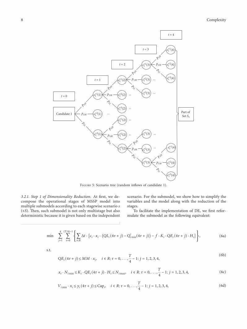

min11139444
j11113944
(T4)minus 1
τ0δ4τ middot 1113896 1113944
iisinRΔt middot ci middot xi middot QLi(4τ + j) minus Qiminprime(4τ + j)( 1113857 minus f middot Ki middot QEi(4τ + j) middot Hi1113858 1113859 + β+
1(j) middot QEi(4τ + j) minus MM middot xi( 1113857
+ β+2(j) middot Ki middot QEi(4τ + j) middot Hi minus Nimax( 1113857 + βminus
2(j) middot Ki middot QEi(4τ + j) middot Hi minus xi middot Nimin( 1113857 + β+3(j) middot yi(4τ + j) minus Capi( 1113857
+ βminus3(j) middot yi(4τ + j) minus Vimin middot xi( 1113857 + β4(j) middot 1113888yi(4τ + j) minus yi(4τ + j minus 1) minus Δt middot 1113888Qiminus 1(4τ + j) + εi(4τ + j)
minus Qi(4τ + j) minus QLi(4τ + j)11138891113889 + β5(j) middot Qi(4τ + j) minus QEi(4τ + j) minus QAi(4τ + j)( 1113857 + β+6(j) middot 1113888QEi(4τ + j)
+ QAi(4τ + j) minus QFimax1113889 + βminus6(j) middot QEi(4τ + j) + QAi(4τ + j) minus QFimin( 1113857
+ β+7(j) middot QLi(4τ + j) minus xi middot Qimax minus 1 minus xi( 1113857 middot Qimin(4τ + j)( 1113857 + βminus
7(j) middot QLi(4τ + j) minus Qimin(4τ + j)( 11138571113897
(9)
Step 3 )us similar to the discounting way of the randomvariables in Section 311 we can integrate the decisionvariables and the parameters under the same season togetherby δ To make the above model concise the so-called lsquoin-tegratedrsquo primal variables are introduced to replace thecorresponding discounted values For example
QLlowasti (j) 1113944
(T4)minus 1
τ0δ4τ middot QLi(4τ + j) j 1 2 3 4 i isin R
(10a)
Qlowastimax 1113944
(T4)minus 1
τ0δ4τ middot Qimax i isin R (10b)
Other integrated primal variables can be given similarlyand all of them take an asterisk at their top right corner)us with the introduction of the lsquointegratedrsquo primal var-iables the symbol 1113936
(T4)minus 1τ0 (middot) in Objective (9) could be re-
moved and then the operational stages 5simT in the submodelcould be compressed into the stages 1sim4 respectively )uswe have
min11139444
j11113896 1113944
iisinRΔt middot ci middot xi middot QL
lowasti (j) minus Q
primelowastimin(j)1113874 1113875 minus f middot Ki middot QE
lowasti (j) middot Hi1113876 1113877
+ β+1(j) middot QE
lowasti (j) minus MM middot xi( 1113857 + β+
2(j) middot Ki middot QElowasti (j) middot Hi minus N
lowastimax( 1113857 + βminus
2(j) middot Ki middot QElowasti (j) middot Hi minus xi middot N
lowastimin( 1113857
+ β+3(j) middot y
lowasti (j) minus Cap
lowasti( 1113857 + βminus
3(j) middot ylowasti (j) minus V
lowastimin middot xi( 1113857
+ β4(j) middot ylowasti (j)minus( y
lowasti (j minus 1)minus Δt middot Q
lowastiminus 1(j) + εlowasti (j) minus Q
lowasti (j) minus QL
lowasti (j)( 11138571113857 + β5(j) middot Q
lowasti (j) minus QE
lowasti (j) minus QA
lowasti (j)( 1113857
+ β+6(j) middot QE
lowasti (j) + QA
lowasti (j) minus QF
lowastimax( 1113857 + βminus
6(j) middot QElowasti (j) + QA
lowasti (j) minus QF
lowastimin( 1113857
+ β+7(j) middot QL
lowasti (j) minus xi middot Q
lowastimax minus 1 minus xi( 1113857 middot Q
lowastimin(j)( 1113857 + βminus
7(j) middot QLlowasti (j) minus Q
lowastimin(j)( 11138571113897
(11)
Step 4 Notice that the above transformation is for thesubmodel which is under a specific scenario SpecificallyStep 2 relaxes the constraints to get a unconstrainted modeland then Step 3 aggregates the multistage for this model
Here we need to extract the relaxed constraints back at firstand then combine the model with each scenario 1113954s (isin1113954S) (seeFigure 5) and the planning stage )us we can get thefollowing intermediate model
10 Complexity
min 1113944iisinR
e middot Capi + 1113944
4
j1Δt middot 1113944
iisinRrlowasti (j) middot Capi
⎛⎝ ⎞⎠
+ 1113944
1113954sisin1113954S
p1113954s middot 11139444
j11113944iisinRΔt middot ci middot xi middot QL
lowast1113954si (j) minus Q
primelowast1113954simin(j)1113874 1113875 minus f middot Ki middot QE
lowast1113954si (j) middot Hi1113876 1113877
(12a)
st
Rmin le 1113944iisinR
xi leR (12b)
Capi leMM middot xi i isin R (12c)
QElowast1113954si (j)leMM middot xi i isin R1113954s isin 1113954S j 1 2 3 4 (12d)
xi middot Nlowastimin leKi middot QE
lowast1113954si (j) middot Hi leN
lowastimax i isin R1113954s isin 1113954S j 1 2 3 4 (12e)
Vlowastimin middot xi ley
lowast1113954si (j)leCaplowasti i isin R1113954s isin 1113954S j 1 2 3 4 (12f)
ylowast1113954si (j) minus y
lowast1113954si (j minus 1) Δt middot Q
lowast1113954siminus 1(j) + εlowast1113954si (j) minus Q
lowast1113954si (j) minus QL
lowast1113954si (j)1113876 1113877
i isin R1113954s isin 1113954S j 1 2 3 4
(12g)
Qlowast1113954si (j) QE
lowast1113954si (j) + QA
lowast1113954si (j) i isin R1113954s isin 1113954S j 1 2 3 4 (12h)
QFlowastimin leQE
lowast1113954si (j) + QA
lowast1113954si (j)leQF
lowastimax i isin R1113954s isin 1113954S j 1 2 3 4 (12i)
Qlowast1113954simin(j)leQL
lowast1113954si (j)le xi middot Q
lowastimax + 1 minus xi( 1113857 middot Q
lowast1113954simin(j) i isin R1113954s isin 1113954S j 1 2 3 4 (12j)
xi isin 0 1 Capi ge 0 i isin R (12k)
in which the primal variables Caplowasti can be given as follows
Caplowasti 1113944
(T4)minus 1
τ0δ4τ middot Capi Capi middot δ0 + δ4 + δ8 + middot middot middot + δTminus 8
+ δTminus 41113872 1113873
Capi middot1 minus δT
1 minus δ4asymp Capi middot
11 minus δ4
i isin R
(12l)in which δTcan be approximated as zero when the number ofstages T is large enough Similarly the parameters rlowasti (j)
could be given as
rlowasti (j) 1113944
(T4)minus 1
τ0δ4τ middot ri(4τ + j) j 1 2 3 4 i isin R
(12m)
We can assume the unit operational cost of candidate i ateach stage t is the same ie ri )en (12m) can be furtherrepresented as
rlowasti (j) ri middot
1 minus δT
1 minus δ4asymp ri middot
11 minus δ4
i isin R (12n)
Moreover it is easy to know that Caplowasti ylowast1113954si (j) QLlowast1113954si (j)QElowast1113954si (j) Qlowast1113954si (j) an dQAlowast1113954si (j) are all nonnegative
Till now along with the stage reduction as shown inSection 311 the T-stage operations of the MSSP model isintegrated into a four-stage model )e correspondingscenario tree of this intermediate model is shown inFigure 5
322 Step 2 of Dimensionality Reduction Further modeltransformation is required due to the stage reduction inSection 312 Notice that j (1 2 3 4) in the intermediatemodel (12) refers to the first four operational stages Here weuse symbol t to replace the corresponding j and then in-tegrate stage t 2 3 4 into the first stage (t 1) as illustratedin Section 312 )e way how to transform is similar to thatin Section 321
We still focus on the operational stage under a specificstagewise scenario )us the corresponding submodel canbe described as follows
Complexity 11
min 11139444
t11113944iisinRΔt middot ci middot xi middot QL
lowasti (t) minus Q
primelowastimin(t)1113874 1113875 minus f middot Ki middot QE
lowasti (t) middot Hi1113876 11138771113882 1113883 (13a)
stQElowasti (t)leMM middot xi i isin R t 1 2 3 4
(13b)
xi middot Nlowastimin leKi middot QE
lowasti (t) middot Hi leN
lowastimax i isin R t 1 2 3 4 (13c)
Vlowastimin middot xi ley
lowasti (t)le
11 minus δ4
middot Capi i isin R t 1 2 3 4 (13d)
ylowasti (t) minus y
lowasti (t minus 1) Δt middot Q
lowastiminus 1(t) + εlowasti (t) minus Q
lowasti (t) minus QL
lowasti (t)1113858 1113859
i isin R t 1 2 3 4(13e)
Qlowasti (t) QE
lowasti (t) + QA
lowasti (t) i isin R t 1 2 3 4 (13f)
QFlowastimin leQE
lowasti (t) + QA
lowasti (t)leQF
lowastimax i isin R t 1 2 3 4 (13g)
Qlowastimin(t)leQL
lowasti (t)le xi middot Q
lowastimax + 1 minus xi( 1113857 middot Q
lowastimin(t) i isin R t 1 2 3 4 (13h)
Step 5 )e discount factor δ is still used to aggregate thevalue of the objective function at stage t (2 3 4) )en theobjective function (13a) is transformed as
min11139444
t1δtminus 1
middot 1113944iisinRΔt middot ci middot xi middot QLi(t) minus Qiminprime (t)( 1113857 minus f middot Ki middot QEi(t) middot Hi1113858 1113859
⎧⎨
⎩
⎫⎬
⎭ (14)
Step 6 Similar to Step 2 use dual multipliers β7+kt (k 1 7) to relax the k-th one of Constraints (13b)sim(13h) ofstage t )us the operational optimization problem under
stage t 1sim4 ((13b)sim(13h) (14)) can be transformed to anunconstrainted one
min11139444
t11113896δtminus 1
middot 1113944iisinRΔt middot ci middot xi middot QL
lowasti (t) minus Q
primelowastimin(t)1113874 1113875 minus f middot Ki middot QE
lowasti (t) middot Hi1113876 1113877
+ β+8t middot QE
lowasti (t) minus MM middot xi( 1113857
+ β+9t middot Ki middot QE
lowasti (t) middot Hi minus N
lowastimax( 1113857 + βminus
9t middot Ki middot QElowasti (t) middot Hi minus xi middot N
lowastimin( 1113857
+ β+10t middot y
lowasti (t) minus
11 minus δ4
middot Capi1113874 1113875 + βminus10t middot y
lowasti (t) minus V
lowastimin middot xi( 1113857
+ β11t middot ylowasti (t) minus y
lowasti (t minus 1) minus Δt middot Q
lowastiminus 1(t) + εlowasti (t) minus Q
lowasti (t) minus QL
lowasti (t)( 1113857( 1113857
+ β12t middot Qlowasti (t) minus QE
lowasti (t) minus QA
lowasti (t)( 1113857
+ β+13t middot QE
lowasti (t) + QA
lowasti (t) minus QF
lowastimax( 1113857
+ βminus13t middot QE
lowasti (t) + QA
lowasti (t) minus QF
lowastimin( 1113857
+ β+14t middot QL
lowasti (t) minus xi middot Q
lowastimax minus 1 minus xi( 1113857 middot Q
lowastimin(t)( 1113857 + βminus
14t middot QLlowasti (t) minus Q
lowastimin(t)( 11138571113897
(15)
12 Complexity
in which the dual multipliers follow the formβ7+kt δtminus 1middotβ7+k Hence problem (15) can further beexpressed as
min11139444
t1δtminus 1
middot 1113896 1113944iisinRΔt middot ci middot xi middot QL
lowasti (t) minus Q
primelowastimin(t)1113874 1113875 minus f middot Ki middot QE
lowasti (t) middot Hi1113876 1113877
+ β+8 middot QE
lowasti (t) minus MM middot xi( 1113857
+ β+9 middot Ki middot QE
lowasti (t) middot Hi minus N
lowastimax( 1113857 + βminus
9 middot Ki middot QElowasti (t) middot Hi minus xi middot N
lowastimin( 1113857
+ β+10 middot y
lowasti (t) minus
11 minus δ4
middot Capi1113874 1113875 + βminus10 middot y
lowasti (t) minus V
lowastimin middot xi( 1113857
+ β11 middot ylowasti (t) minus y
lowasti (t minus 1) minus Δt middot Q
lowastiminus 1(t) + εlowasti (t) minus Q
lowasti (t) minus QL
lowasti (t)( 1113857( 1113857
+ β12 middot Qlowasti (t) minus QE
lowasti (t) minus QA
lowasti (t)( 1113857 + β+
13 middot QElowasti (t) + QA
lowasti (t) minus QF
lowastimax( 1113857
+ βminus13 middot QE
lowasti (t) + QA
lowasti (t) minus QF
lowastimin( 1113857
+ β+14 middot QL
lowasti (t) minus xi middot Q
lowastimax minus 1 minus xi( 1113857 middot Q
lowastimin(t)( 1113857 + βminus
14 middot QLlowasti (t) minus Q
lowastimin(t)( 11138571113897
(16)
Step 7 Similar to Step 3 the ldquointegratedrdquo primal variablesare introduced to replace the corresponding discountedvalues respectively TakingQLi(t) andQimax as examples wehave
QLlowastlowasti 1113944
4
t1δtminus 1
middot QLlowasti (t) i isin R (17a)
Qlowastlowastimax 1113944
4
t1δtminus 1
middot Qlowastimax i isin R (17b)
Here all the primal variables have double asterisks intheir top right corner )us
min1113944iisinR
1113896Δt middot ci middot xi middot QLlowastlowasti minus Q
primelowastlowastimin1113874 1113875 minus f middot Ki middot QE
lowastlowasti middot Hi1113876 1113877 + β+
8 middot QElowastlowasti minus MM middot xi( 1113857
+ β+9 middot Ki middot QE
lowastlowasti middot Hi minus N
lowastlowastimax( 1113857 + βminus
9 middot Ki middot QElowastlowasti middot Hi minus xi middot N
lowastlowastimin( 1113857
+ β+10 middot y
lowastlowasti minus
11 minus δ4
middot Caplowasti1113874 1113875 + βminus10 middot y
lowastlowasti minus V
lowastlowastimin middot xi( 1113857 + β11 middot y
lowastlowasti minus y
lowastlowasti (0)( minus Δt middot Q
lowastlowastiminus 1 + εlowastlowasti minus Q
lowastlowasti minus QL
lowastlowasti( 11138571113857
+ β12 middot Qlowastlowasti minus QE
lowastlowasti minus QA
lowastlowasti( 1113857 + β+
13 middot QElowastlowasti + QA
lowastlowasti minus QF
lowastlowastimax( 1113857 + βminus
13 middot QElowastlowasti + QA
lowastlowasti minus QF
lowastlowastimin( 1113857
+ β+14 middot QL
lowastlowasti minus xi middot Q
lowastlowastimax minus 1 minus xi( 1113857 middot Q
lowastlowastimin( 1113857 + βminus
14 middot QLlowastlowasti minus Q
lowastlowastimin( 11138571113897
(18)
in which
Caplowasti 11139444
t1δtminus 1
middot Capi 1 minus δ4
1 minus δmiddot Capi i isin R (19)
and for each i (isinR) ylowastlowasti is a discounted value that can beexpressed as
ylowastlowasti 1113944
4
t1δtminus 1
middot ylowasti (t) 1113944
4
t1δtminus 1
middot 1113944
(T4)minus 1
τ0δ4τ middot yi(4τ + t)
(20)
From (20) we have
Complexity 13
δ middot ylowastlowasti 1113944
4
t1δt
middot 1113944
(T4)minus 1
τ0δ4τ middot yi(4τ + t) (21)
Refer to (20) the discounted value ylowastlowasti (0) can bedenoted as
ylowastlowasti (0) 1113944
4
t1δtminus 1
middot ylowasti (t minus 1) 1113944
4
t1δtminus 1
middot 1113944
(T4)minus 1
τ0δ4τ middot yi(4τ + t minus 1)
(22)
From (21) and (22) we have
ylowastlowasti (0) δ middot y
lowastlowasti + δ0 middot yi(0) minus δT
middot yi(T) (23)
Using (23) to replace ylowastlowasti (0) in (18) we have the dis-counted objective as follows
min1113944iisinR
1113896Δt middot ci middot xi middot QLlowastlowasti minus Q
rsquolowastlowastimin1113872 1113873 minus f middot Ki middot QE
lowastlowasti middot Hi1113960 1113961
+ β+8 middot QE
lowastlowasti minus MM middot xi( 1113857
+ β+9 middot Ki middot QE
lowastlowasti middot Hi minus N
lowastlowastimax( 1113857 + βminus
9 middot Ki middot QElowastlowasti middot Hi minus xi middot N
lowastlowastimin( 1113857
+ β+10 middot y
lowastlowasti minus
11 minus δ4
middot1 minus δ4
1 minus δmiddot Capi1113888 1113889 + βminus
10 middot ylowastlowasti minus V
lowastlowastimin middot xi( 1113857
+ β11 middot ylowastlowasti minus δ middot y
lowastlowasti minus yi(0) + δT
middot1113872 yi(T)minus Δt middot Qlowastlowastiminus 1 + εlowastlowasti minus Q
lowastlowasti minus QL
lowastlowasti( 11138571113857
+ β12 middot Qlowastlowasti minus QE
lowastlowasti minus QA
lowastlowasti( 1113857
+ β+13 middot QE
lowastlowasti + QA
lowastlowasti minus QF
lowastlowastimax( 1113857 + βminus
13 middot QElowastlowasti + QA
lowastlowasti minus QF
lowastlowastimin( 1113857
+ β+14 middot QL
lowastlowasti minus xi middot Q
lowastlowastimax minus 1 minus xi( 1113857 middot Q
lowastlowastimin( 1113857 + βminus
14 middot QLlowastlowasti minus Q
lowastlowastimin( 11138571113897
(24)
Similarly δT in (24) can be approximated as zero due tothe large T )en by extracting the relaxed constraints fromthe above objective function we have
min 1113944iisinRΔt middot ci middot xi middot QL
lowastlowasti minus Q
rsquolowastlowastimin1113872 1113873 minus f middot Ki middot QE
lowastlowasti middot Hi1113960 1113961
(25a)
stQElowastlowasti leMM middot xi i isin R
(25b)
xi middot Nlowastlowastimin leKi middot QE
lowastlowasti middot Hi leN
lowastlowastimax i isin R (25c)
Vlowastlowastimin middot xi ley
lowastlowasti le
11 minus δ
middot Capi i isin R (25d)
(1 minus δ)ylowastlowasti minus yi(0) Δt middot Q
lowastlowastiminus 1 + εlowastlowasti minus Q
lowastlowasti minus QL
lowastlowasti( 1113857
i isin R
(25e)
Qlowastlowasti QE
lowastlowasti + QA
lowastlowasti i isin R (25f)
QFlowastlowastimin leQE
lowastlowasti + QA
lowastlowasti leQF
lowastlowastimax i isin R (25g)
Qlowastlowastimin leQL
lowastlowasti le xi middot Q
lowastlowastimax + 1 minus xi( 1113857 middot Q
lowastlowastimin i isin R
(25h)
Step 8 Combine the above model with each scenario 1113954s (isin1113954S)which is given in Section 312 and then integrate with theplanning stage of the original MSSP model )us the finalDE model which is a two-stage stochastic program is de-veloped as (26a)sim(26k)min1113944
iisinRe middot Capi + Δt middot 1113944
iisinRrlowastlowasti middot Capi( 1113857
+ 1113944
1113954sisin1113954S
p1113954s
middot 1113944iisinRΔt middot ci middot xi middot QL
1113954si minus Qprimelowastlowast1113954simin1113874 1113875 minus f middot Ki middot QE
1113954si middot Hi1113876 1113877
⎧⎨
⎩
⎫⎬
⎭
(26a)
st
Rmin le 1113944iisinR
xi leR (26b)
Capi leMM middot xi i isin R (26c)
14 Complexity
QE1113954si leMM middot xi 1113954s isin 1113954S i isin R (26d)
xi middot Nlowastlowastimin leKi middot QE
1113954si middot Hi leN
lowastlowastimax 1113954s isin 1113954S i isin R
(26e)
Vlowastlowastimin middot xi ley
1113954si le
11 minus δ
middot Capi 1113954s isin 1113954S i isin R (26f)
(1 minus δ)y1113954si minus yiprime Δt middot Q
1113954siminus 1 + εlowastlowast1113954si minus Q
1113954si minus QL
1113954si1113876 1113877 1113954s isin 1113954S i isin R
(26g)
Q1113954si QE
1113954si + QA
1113954si 1113954s isin 1113954S i isin R (26h)
QFlowastlowastimin leQE
1113954si + QA
1113954si leQF
lowastlowastimax 1113954s isin 1113954S i isin R (26i)
Candidate 1Candidate 2
Candidate 3
Candidate 4
Candidate 5
The basin in upstream of Yangtze River
Tributary 1
Tributary 2
Tributary 4
Tributary 3
Demand area
Figure 6 Illustration of hydropower station candidate in upstream of Yangtze river
Table 3 Related parameters of hydropower station candidates
Candidate i Ki (kg(m2middots2)) Nimin (KW) Nimax (KW) Hi (m) ci (RMBm3) ri (RMB(m3middotyear)) Qimax (m3 times108h)1 84 2546250 5092500 105 01 006 046762 84 1506750 3013500 93 0125 0072 085503 84 1500000 3000000 90 015 005 051774 84 3742500 7485000 110 0175 008 046625 84 2625000 5250000 112 02 01 03301
Table 4 Minimum storage and limitation of water flows of hy-dropower station candidates
Candidatei
Vimin(m3 times108)
QFimin (m3 times108h)
QFimax (m3 times108h)
1 00311 00648 157322 00213 00468 179283 00131 00432 042484 00420 01620 355685 00115 00396 06912
Table 5 Random water inflows in each seasonal stage of eachhydropower station candidate
Candidate i Inflows levelWater inflows (m3 times107h)
Spring Summer Autumn Winter
1 H 12846 57276 22020 02031L 09867 43995 16914 01560
2 H 05932 16312 06677 00985L 04589 12617 05165 00762
3 H 05653 12849 06739 00969L 04441 10093 05294 00762
4 H 03645 05958 03356 00930L 02575 04209 02371 00657
5 H 06900 11642 05710 01515L 06482 10936 05363 01423
Probability H 04 07 055 025L 06 03 045 075
Table 6 Predicted water inflows in each seasonal stage
Candidatei
Stage (t 1 2 3 4)Spring Summer Autumn Winter
Water inflowsεi(t) (m3 times107h)
1 11059 53292 19722 016782 05126 15203 05997 008173 04926 12202 06089 008134 03003 05433 02912 007255 06649 11431 05554 01446
Complexity 15
Qlowastlowast1113954simin leQL
1113954si lexi middot Q
lowastlowastimax + 1 minus xi( 1113857 middot Q
lowastlowast1113954simin 1113954s isin 1113954S i isin R
(26j)
Capi y1113954si QL
1113954si QE
1113954si Q
1113954si QA
1113954si ge 0 xi isin 0 1 i isin R1113954s isin 1113954S
(26k)
in which the discounted value of water inflows and demandsεlowastlowast1113954si and Qlowastlowast1113954simin (i isinR) can be obtained similar to the way usedin formula (3) Besides rlowastlowasti in (26a) is an integrated variable
rlowastlowasti 1113944
4
t1δtminus 1
middot rlowasti (t) i isin R (26l)
Moreover for simplicity the double asterisks of thedecision variables are omitted
After transformation the planning decisions xi and Capiremain unchanged while the operational stages are aggre-gated )erefore the proposed approach not only keeps thefuture impacts but also reduces the solving complexity
4 Experimental Study
To validate the applicability of our proposed approach wegive the data of a case in Section 41 at first )en based onthis case we compare our approach with the MSSP model inthe small-scale setting in Section 42 Furthermore we applyour approach to an overlong-term case in Section 43 andfinally implement sensitivity analysis in Section 44
41 Description of the Case Yangtze River flows through 11provinces in China with a drainage area of 18 million squarekilometers )e whole river can be divided into the up-stream midstream and downstream among which thebasin with a length of 1030 km in upstream is studied hereAccording to Wang et al [45] five hydropower stationcandidates could be considered in this basin Its schema-tization is shown in Figure 6 which also involves the maintributaries
Among the five hydropower station candidates at leasttwo of them should be chosen in the plan Unit constructionfee (e) and unit profit of power generation (f ) in Table 1 areset to be 509 (RMBm3) and 025 (RMBKWh) respectively[46] Related parameters regarding five candidates are dis-played in Table 3 Once the hydropower station candidate ischosen the planned lowest water storage and upper andlower limit of water discharge are shown in Table 4 )einitial water flows from upstream to each hydropowerstation candidate is set to be 02141 00988 00942 00429and 01080 (m3 times108h) respectively And the initial waterstorage of each chosen hydropower station is assumed as thetwice of the lowest water storage
42 Comparison with the MSSP Model by Small-Scale Cases)e developed DE model is an approximate version of theMSSP model (1) In this section we aim to evaluate theperformance of our approach by comparing the planningdecisions as well as the operational performance with theseof the MSSP model Due to the curse of dimensionality facedby the MSSP model we consider small-scale cases based onSection 41
421 Parameters in Small-Scale Experiments To limit thedimensionality here we set the planning horizon as 1 2 and3 years respectively According to the seasonal features ofwhich one year is divided into four stages spring (March toMay) summer (June to August) autumn (September toNovember) and winter (December to February) )en eachstage has 2160 (h) (ie Δt) )us the number of operationalstages T is 4 8 and 12 respectively Besides we merelyconsider the uncertainty caused by water inflows Two kindsof stochastic outside water inflows (H L) as well as the
Table 8 Estimation gaps of the DE model
Discount factor δPlanning stages
T 4 T 8 T12099 2553 2251 1994095 1789 671 minus 299090 872 minus 976 minus 2432085 minus 051 minus 2320 minus 3973080 minus 916 minus 3434 minus 5097075 minus 1729 minus 4392 minus 5959070 minus 2472 minus 5199 minus 6637065 minus 3144 minus 5862 minus 7161060 minus 3753 minus 6402 minus 7564
Table 9 Average computational time (ms) of both models
Model T 4 T 8 T12DE model 122400 120644 117022MSSP model 30022 309556 15937322
Table 10 Probabilistic distributions of water inflows and demandsin each seasonal stage
Stage Water inflows (p1H p1Mp1L)
Water demands (p2Hp2L)
Spring (02 04 04) (05 05)Summer (05 04 01) (065 035)Autumn (03 05 02) (06 04)Winter (01 03 06) (03 07)
Table 7 Predicted water demands in each seasonal stage
Candidatei
Stage (t 1 2 3 4)Spring Summer Autumn Winter
WaterdemandsQimin(t)
(m3 times106h)
1 01871 02299 02196 012182 03420 04204 04016 022283 02071 02546 02432 013494 01865 02292 02189 012155 01321 01623 01551 00860
16 Complexity
corresponding probabilities (p1H p1L) in each seasonal stageare given in Table 5 )e constant water inflows and waterdemands used in the simplification are displayed in Tables 6and 7 respectively )e acceptance level of the water spill isassumed as twice of the demands
Because the random inflows fluctuate with seasons weassume the water inflows of each candidate take the sameuncertain level in each season )us for the MSSP model16(24) 256(28) and 4096(212) stagewise scenarios areconstructed respectively Furthermore according to thegeneration and simplification process of the scenario setdisplayed in Section 31 16 scenarios are generated for thetwo-stage DE model Assume that spring is the first oper-ational season)e discount factor δ used in the DEmodel isset to be 099 095 060 respectively
422 Computational Results We optimally solve the DEmodel and the MSSP model by IBM ILOG CPLEX 1263 ona PC with 8GB memory and a CPU at 25GHz
It is found that the DE model can generate the sameplanning results with the MSSP model for all these small-scale cases Besides in terms of the operations the DEmodel considers the multistage operational impacts by theaggregated way Hence it is interesting to observe howaccurate the DE model is in the estimation of the futureoperational performance of the cascade hydropowersystem We use DE_2nd and MSSP_2nd to denote theoperational performance generated by the DE model andthe MSSP model respectively Table 8 displays the esti-mation gap ((DE_2nd-MSSP_2nd)MSSP_2nd) underdifferent discount factors
High Middle Low
Spring Summer Autumn Winter Spring Summer Autumn Winter Spring Summer Autumn Winter
Prec
ipita
tion
(m3 times
107 h
)
4
35
3
25
2
15
1
05
0
1 0867505468054120429203378
38679150351230207015
057
148706155064520395102795
0137200908009280109500742
0545103702037240396802912
2430310181084640648704913
Stage
0934304168044390365402409
0086200615006390101300639
0222601937020350364502445
0992705327046250595804126
0381602181024260335602023
0035200322003490093
00537
2345
Figure 7 High middle low-level precipitation in each seasonal stage of each hydropower station candidate
Spring Summer Autumn Winter Spring Summer Autumn Winter Spring Summer Autumn Winter
1 12735 56781 2183 02014 10188 45425 17464 01611 07641 34068 13098 012082 04419 12151 04974 00734 03535 09721 03979 00587 02651 07291 02984 00443 0401 09113 0478 00688 03208 07291 03824 0055 02406 05468 02868 004134 0 0 0 0 0 0 0 0 0 0 0 05 07425 12527 06144 0163 0594 10022 04915 01304 04455 07516 03686 00978
0
1
2
3
4
5
6
Trib
utar
y (m
3 times 1
07 h)
Stage
High Middle Low
Figure 8 High middle low-level tributary in each seasonal stage of each hydropower station candidate
Complexity 17
Table 11 Predicted water inflows and demands in each seasonal stage
Candidate iStage (t 1 2 3 4)
Spring Summer Autumn Winter
Water inflows εi(t) (m3 times107h)
1 14484 80021 27796 020172 06708 22816 08445 009823 06433 18019 08559 009754 03904 06698 03683 009715 08462 16252 07486 01729
Water demands Qimin(t) (m3 times106h)
1 01871 02299 02196 012182 03420 04204 04016 022283 02071 02546 02432 013494 01865 02292 02189 012155 01321 01623 01551 00860
Table 12 Planning decisions and the costbenefit
Candidate i Capi (m3 times108) Operational cost (RMBtimes 108) Penalty cost (RMBtimes 108) Benefit (RMBtimes 108)1 0214 0063 347191 5500024 0043 0017 0 8084015 0108 0053 0 567013
Table 13 Operational decisions under scenario 16
Candidate i 1 2 3 4 5QL16
i (m3 times108h) 2154 0066 0040 0036 0026QE16
i (m3h) 115476 0 0 162013 111607QA16
i (m3 times108h) 4690 6714 8496 9246 11014y16
i (m3 times108) 4282 0 0 0858 2161Q16
i (m3 times108h) 4691 6714 8496 9248 11015
Table 14 Operational decisions under scenario 1281
Candidate i 1 2 3 4 5QL1281
i (m3 times108h) 0874 0073 0044 0040 0028QE1281
i (m3h) 115476 0 0 162013 111607QA1281
i (m3 times108h) 5171 6936 8496 9219 10847y1281
i (m3 times108) 4282 0 0 0858 0230Q1281
i (m3 times108h) 5172 6936 8496 9221 10848
Spring Summer Autumn Winter Spring Summer Autumn Winter1 02368 02703 02644 01722 01433 01634 01599 010452 04275 04888 04781 03094 02565 02933 02868 018563 02589 0296 02895 01873 01553 01776 01737 011244 02331 02665 02606 01687 01399 01599 01564 010125 01651 01887 01846 01195 0099 01132 01107 00717
0
01
02
03
04
05
06
Stage
High Low
Dem
and
(m3 times1
06 h)
Figure 9 High low-level water demand in each seasonal stage of each hydropower station candidate
18 Complexity
It is found that the operational performance gener-ated by the DE model significantly varies with the dis-count factors Specifically when δ is large more futureimpacts would be taken into account which results in theoverestimation Hence the estimation gap is positiveWith the decrease of δ less future performance would bediscounted )us the estimation gap tends to be negativegradually It also means that the DE model can generateaccurate estimation of the future operational perfor-mance by choosing the appropriate discount factor
Moreover the computational time of the DP modeloutperforms that of the MSSP model greatly especially whenthe horizon is large as shown in Table 9
In summary the DP model can yield the same locationdecisions with the MSSP model and the accurate estimation
of the future operational performance by choosing a suitablediscount factor while less calculational time is required
43RealCase Study Section 42 validates the effectiveness ofour proposed DE model in the small-scale setting In thissection we further apply our approach to a large-scale caseto illustrate its applicability
431 Parameters in the Large-Scale Case Based on the casegiven in Section 41 we consider the 40-year planninghorizon (ie T160) )ree kinds of stochastic water in-flows (H M and L) and two kinds of stochastic water de-mands (H L) are taken into account in each seasonal stage)e corresponding probabilities of two random variables are(p1H p1M p1L) and (p2H p2L) as shown in Table 10 Refer to
Table 15 Corresponding cost terms and benefit
Operationalstages
Candidatei
Total performance(RMBtimes 108)
Operational cost(RMBtimes 108)
Penalty cost(RMBtimes 108)
Power generation(RMBtimes 108)
T 40
1 471396 0063 77453 5500024 808165 0017 0 8084015 566410 0053 0 567013
Total 1845971 0134 77453 1925416
T 80
1 236358 0063 312491 5500024 808165 0017 0 8084015 566410 0053 0 567013
Total 1610933 0134 312491 1925416
T120
1 205604 0063 343245 5500024 808165 0017 0 8084015 566410 0053 0 567013
Total 1580179 0134 343245 1925416
T160
1 201653 0063 347196 5500024 808165 0017 0 8084015 566410 0053 0 567013
Total 1576228 0134 347196 1925416
T 200
1 201150 0063 347699 5500024 808165 0017 0 8084015 566410 0053 0 567013
Total 1575725 0134 347699 1925416
0010203040506070809
04
δ =
099
δ =
098
δ =
097
δ =
096
δ =
095
δ =
094
δ =
093
δ =
092
δ =
091
δ =
090
δ =
089
δ =
088
14
24
34
44
54
64
74
Tota
l per
form
ance
pro
fit o
f pow
erge
nera
tion
pena
lty (R
MB)
1e12
Ope
ratio
nal c
ost (
RMB)
1e7
Change of the discount factor
Operational costTotal performance
Profit of power generationPenalty cost
Figure 10 Cost and profit of power generation under the differentdiscount factors
40
60
50
40
30
20
10
080 120 160
Pena
lty co
st (R
MB)
Change of periods
δ = 093
δ = 091δ = 092
δ = 089δ = 090δ = 088
1e9
δ = 096δ = 095δ = 094
δ = 099δ = 098δ = 097
Figure 11 Penalty cost under the different discount factors andplanning horizons
Complexity 19
Wang et al [47] and Yang and Zhang [48] Uncertain waterinflows which mainly include precipitation and water frommain tributaries (drainage areas larger than ten thousandsquare kilometers) are given in Figures 7 (precipitation) and8 (tributary) respectively Random demands are given inFigure 9 Besides the predicted water inflows and demandsused in the DEmodel are shown in Table 11 and the randomacceptance level of water spill is also assumed as twice of thecorresponding demands
)us the number of stagewise scenarios in the MSSPmodel is up to 6160(asymp3193times10124) which is impossible tohandle exactly By the DE model the number of scenarios isreduced to 1296 )e discount factor δ is set to be 095 here
432 Computational Results of the DE Model )e optimalsolution of the DE model can be obtained by within 2047(ms) by IBM ILOG CPLEX 1263 in which Candidates 1 4and 5 are selected Table 12 shows the capacity decisions andthe operational performance including the operational costthe penalty cost and the profit of power generation of eachselected candidate )e total performance value includingthe planning stage and the operational stages is 1576times1011(RMB)
We further observe two extreme scenarios One is sce-nario 16 (high-level inflows and low-level demands in allfour seasons) and another scenario is 1281 (low-level in-flows and high-level demands in all four seasons) )ecorresponding scenario-dependent operational results offive hydropower station candidates under two scenarios areshown in Tables 13 and 14 respectively
As shown in Tables 13 and 14 the daily schedulingstrategies would be adjusted according to different scenariosFirst in terms of loss flow (QL) when scenario 16 happensthe value is relatively high in hydropower station 1 toprevent the flood (see Table 13) While if scenario 1281occurs the loss flow merely satisfies demand (see Table 14))en regarding water storage (y) the value is high in hy-dropower station 5 under scenario 16 due to the high-levelinflows and the low-level demands However scenario 1281
which represents the low-level inflows and the high-leveldemands requires hydropower stations to utilize theirstorage efficiently and then results in low water storageFurthermore in the computational results the schedulingstrategies would ensure that the values of water discharge(Q) are between the upper and lower limits in both scenariosmaking it capable of preventing flood and drainage Noticethat the water discharges of power generation under twoscenarios are the same and the upper limit of output hasbeen reached under both scenarios )us the schedulingstrategies can always pursue maximum benefits of powergeneration under different scenarios In such a way theproposed DE model can optimize the global performance inthe uncertain setting
44 Sensitivity Analysis In this section we carry out thesensitivity analysis to reveal how critical parameters influ-ence the strategic decisions and the performance of thecascade hydropower stations Because one of the merits is tohandle overlong stochasticity by the idea of aggregation twonatural concerns are how long and how much are dis-counted Here we focus on the planning horizon (T) and thediscount factor (δ)
441 Sensitivity Analysis of the Planning Horizon )eplanning horizon (T) is one of the main factors causing thecurse of dimensionality [19 41] )e DE model aggregatesthe multiple operational stages but T would influence theresults of the model transformation Hence we focus on thelength of the planning horizon here Considering the long-lasting effects of the location decisions we set the length ofthe planning horizon as 10 20 30 40 and 50 years re-spectively )at is we consider T 40 80 120 160 and 200Other parameters are the same as those in Section 43
After calculation it is found that the decisions of locationand capacity under different T which are the planningresults we care about in our study are the same as these ofT160 (see Table 12) It means these planning horizonswould not alter the strategic decisions of the DE model
Furthermore the cost terms and the profit of powergeneration are displayed in Table 15 It is found that theoperational cost and the profit of power generation remainunchanged while the penalty approaches to be stable withthe increase of T Specifically the operational cost is thecapacity-related cost within the planning horizon In the DEmodel the impacts of the capacity-related cost are aggre-gated by δT respectively When T is extremely large δT canbe approximated as zero see (12l) and (12n) Hence theoperational cost keeps unchanged Besides to calculate thebenefit of the power generation it is found that the maxi-mum output is reached in our cases )us after aggregationby δT the benefit of the power generation also remainsconstant Moreover the penalty of hydropower station 4 and5 are zero because the loss flows are smaller than the cor-responding penalty thresholds However Twould influenceylowastlowasti (see (20)) at first and then the loss flow by constraints(25e) Hence the penalty of hydropower station 1 wouldincrease gradually until coming to be stable
10110210310410510610710810910
40 80 120 160
Tota
l per
form
ance
(RM
B)
1e9
Change of periods
δ = 096δ = 095δ = 094
δ = 099δ = 098δ = 097
δ = 093
δ = 091δ = 092
δ = 089δ = 090δ = 088
Figure 12 Total performance under the different discount factorsand planning horizons
20 Complexity
Based on the above three terms with the increase of Tthe total performance also shows a trend of increasing firstand then approaches to be stable )is result coincides withthe essence of the DE model Specifically the farther thefuture is the fewer the impacts would be taken into account)us the results would close to be stable finally It is also inaccord with the decision-making in the real-world ie thecoming future would be put more emphasis than thesuperfar future Hence when T is large enough the calcu-lational results of the DE model would tend to be stable Itmeans that the DEmodel could describe the steady results oflong-term stochastic operations )us for the decision-makers (DMs) it is not necessary to increase the planninghorizon infinitely
442 Sensitivity Analysis of the Discount FactorDiscount factor (δ) is an exogenous variable introduced bythe DE model to help to reduce dimensionality In Section42 we have shown that the DE model can generate accurateoperational performance estimation by selecting appropriateδ In this section we further explore the impacts of thediscount factor in the large-scale setting We vary it as 099098 088 Other parameters are the same as those ofSection 43
)e calculational results show the discount factors in thevalue range above will not influence the final strategic de-cisions Besides the operational cost the penalty cost theprofit of power generation and the total performance underdifferent discount factors are shown in Figure 10 Firstly it isshown that with the decrease of the discount factor both theoperational cost and the profit decline with a decreasingspeed since they are discounted more Moreover in terms ofthe penalty cost it remains zero when δ is large (099))is isbecause the discounted penalty threshold also decreases butis still larger than the loss flow )en the penalty cost in-creases significantly with the decline of δ to 098 )e reasonis that the discounted penalty threshold begins to be smallerthan the loss flow leading to the larger penalty Finally withits continuous decrease (less than 098) δ dominates thepenalty term which makes the aggregated penalty smaller
)ese results indicate different discount factors will notinfluence the location decisions but result in the variation ofthe operational performance Hence the DMs shouldcarefully choose the discount factor if they want to get anaccurate estimation of the operational performance
443 Mutual Effects of Two Factors We further investigatethe mutual impacts of two factors on decisions and objectiveterms We set T as 40 80 120 160 and 200 and δ as 099098 088 and then calculate the model under eachcombination of two kinds of parameters
From the calculational results we find that the locationsand capacities of hydropower stations remain unchangedunder the different combinations of planning horizon anddiscount factor Given a δ the operational cost and the profitof power generation will not be influenced by the change ofT which is similar to Table 15 Hence we focus on thepenalty and the total operational performance
Figure 11 shows the varying pattern of the penalty withthe decrease of δ under each T Specifically the penaltyincreases first and then decreases )e reason is the same asthat in Figure 10 However with the increase of T the peakpoint would appear earlier It is because bigger T can bringsignificant discounting effects due to δT
Furthermore we show the change of the total perfor-mance in Figure 12)e variations under different Tare verysimilar Specifically with the decline of δ the total perfor-mance gradually decreases and finally tends to be stableBesides as δ becomes smaller the total performance wouldreach its steady state within a shorter planning horizonspecifically around 120 periods when δ 096 and aroundmerely 40 periods when δ 090 )us we conclude thatwhen the low δ is considered the DMs could only consider arelatively shorter planning horizon since the impacts in thelong-term future would be significantly discounted
5 Conclusions and Future Research Directions
)e integrated planning of cascade hydropower stationswhich takes the operational strategies under future un-certainty into account can bring global benefit An MSSPmodel is developed to deal with the location and capacitydecisions of cascade hydropower stations with the consid-eration of the expected long-term performance To addressthe computational issue caused by the overlong stochasticitya dimensionality reduction approach based on DE isdesigned to transform the MSSP model into a two-stagestochastic programming model in which future impactsremain by aggregating the operational stages together )usthe optimization of the large-scale hydropower stationscould be addressed regardless of the number of operationalstages
Experiments based on Yangtze River in China areimplemented First by the comparison with the MSSPmodel under the small-sized cases it is found that ourapproach can obtain the same planning results and accurateestimation for future operational performance with a shortcomputational time )en a large-scale case is studied toshow how the approach is applied to solve a practicalproblem Moreover to evaluate the influence of criticalparameters in the proposed DE model sensitivity analysis isconducted based on the planning horizon and the discountfactor)e results reveal that our model is robust to differentparameter settings to obtain stable location-related planningresults while the estimation of the future performancewould be influenced by the planning horizon and the dis-count factor )e corresponding observations and impli-cations are also obtained from the results
In the future we can extend our study in the followingaspects First the discount factor plays an important role inour study Specifically it not only discounts the futureimpacts to get the so-called net present value but also has theinternal relationship between the dual multipliers )us itinfluences the accuracy of the future estimation of the DEmodel In this paper we follow the way of Grinold [42] andKing and Wallace [43] to give the discount factor directlyBut how to select the appropriate discount factor to get
Complexity 21
better performance estimation should be considered in thefuture study It is a hard issue but deserves further effortSecond the minimum installed power and the nonlinearitylike the stage-storage curve are ignored in this paper )econsideration of these requirements and constraints couldhelp to improve the applicability of our approach to practicalproblems which leaves certain spaces for future study Fi-nally in this paper the impacts of time-varying stochasticoperations are considered in the form of expected valueAnother popular way is to formulate the objective of Value-at-Risk or Conditional Value-at-Risk to incorporate theDMsrsquo risk attitudes )en is it possible to utilize thecharacteristics of Value-at-Risk or Conditional Value-at-Risk to facilitate our scenario tree reduction It is anotherinteresting research direction
Data Availability
All data included in this paper are available upon request bycontact with the corresponding author
Conflicts of Interest
)e authors declare that there are no conflicts of interestregarding the publication of this paper
Acknowledgments
)e authors wish to express their gratitude to the fiveanonymous referees for their constructive criticism which ledto substantial improvements of the paper )is research waspartly supported by the National Natural Science Foundationof China (Grant no 71971053 71832001 71572033) and theMOE (Ministry of Education in China) Project of Humanitiesand Social Sciences (Grant no 18YJA630129)
References
[1] A Afshar F Sharifi and M R Jalali ldquoNon-dominated ar-chiving multi-colony ant algorithm for multi-objective op-timization application to multi-purpose reservoir operationrdquoEngineering Optimization vol 41 no 4 pp 313ndash325 2009
[2] P Fraenkel O Paish V Bokalders A Harvey andA E Brown Micro-Hydro Power A Guide for DevelopmentWorkers IT Publications Ltd London UK 1999
[3] G Eiger and U Shamir ldquoOptimal operation of reservoirs bystochastic programmingrdquo Engineering Optimization vol 17no 4 pp 293ndash312 1991
[4] A Gjelsvik B Mo and A Haugstad ldquoLong- and medium-term operations planning and stochastic modelling in hydro-dominated power systems based on stochastic dual dynamicprogrammingrdquo in Handbook of Power Systems I EnergySystems Section 2 Springer Berlin Germany 2010
[5] C Cheng S Wang K-W Chau and XWu ldquoParallel discretedifferential dynamic programming for multireservoir oper-ationrdquo Environmental Modelling amp Software vol 57pp 152ndash164 2014
[6] C Wang J Zhou P Lu and L Yuan ldquoLong-term schedulingof large cascade hydropower stations in Jinsha river ChinardquoEnergy Conversion and Management vol 90 no 15pp 476ndash487 2015
[7] Y Xu and Y Mei ldquoA modified water cycle algorithm for long-term multi-reservoir optimizationrdquo Applied Soft Computingvol 71 pp 317ndash332 2018
[8] D G Larentis W Collischonn F Olivera and C E M TuccildquoGIS-based procedures for hydropower potential spottingrdquoEnergy vol 35 no 10 pp 4237ndash4243 2010
[9] B C Kusre D C Baruah P K Bordoloi and S C PatraldquoAssessment of hydropower potential using GIS and hy-drological modeling technique in Kopili river basin in Assam(India)rdquo Applied Energy vol 87 no 1 pp 298ndash309 2010
[10] B SerpoushM Khanian and A Shamsai ldquoHydropower plantsite spotting using geographic information system and aMATLAB based algorithmrdquo Journal of Cleaner Productionvol 152 pp 7ndash16 2017
[11] A Z Zaidi and M Khan ldquoIdentifying high potential locationsfor run-of-the-river hydroelectric power plants using GIS anddigital elevation modelsrdquo Renewable and Sustainable EnergyReviews vol 89 pp 106ndash116 2018
[12] J Hosnar and A Kovac-Kralj ldquoMathematical modelling andMINLP programming of a hydro system for power genera-tionrdquo Journal of Cleaner Production vol 65 no 4 pp 194ndash201 2014
[13] C Loannidou and J R OrsquoHanley ldquoEco-friendly location ofsmall hydropowerrdquo European Journal of Operational Re-search vol 264 pp 907ndash918 2018
[14] D A G Vieira L S M Guedes A C Lisboa andR R Saldanha ldquoFormulations for hydroelectric energyproduction with optimality conditionsrdquo Energy Conversionand Management vol 89 pp 781ndash788 2015
[15] C T Cheng J J Shen and X Y Wu ldquoShort-term schedulingfor large-scale cascaded hydropower systems with multi-vibration zones of high headrdquo Journal of Water ResourcePlanning and Management vol 138 no 3 pp 257ndash267 2012
[16] C Li J Zhou S Ouyang X Ding and L Chen ldquoImproveddecomposition-coordination and discrete differential dy-namic programming for optimization of large-scale hydro-power systemrdquo Energy Conversion and Management vol 84pp 363ndash373 2014
[17] X Li J Wei T Li G Wang and W W-G Yeh ldquoA paralleldynamic programming algorithm for multi-reservoir systemoptimizationrdquo Advances in Water Resources vol 67 no 4pp 1ndash15 2014b
[18] Z-K Feng W-J Niu C-T Cheng and S-L Liao ldquoHy-dropower system operation optimization by discrete differ-ential dynamic programming based on orthogonalexperiment designrdquo Energy vol 126 pp 720ndash732 2017
[19] Z-K Feng W-J Niu C-T Cheng and X-Y Wu ldquoOpti-mization of hydropower system operation by uniform dy-namic programming for dimensionality reductionrdquo Energyvol 134 pp 718ndash730 2017
[20] C Cheng J Shen X Wu and K-W Chau ldquoShort-termhydroscheduling with discrepant objectives using multi-stepprogressive optimality algorithmrdquo JAWRA Journal of theAmerican Water Resources Association vol 48 no 3pp 464ndash479 2012
[21] Z-K Feng W-J Niu and C-T Cheng ldquoOptimizing elec-trical power production of hydropower system by uniformprogressive optimality algorithm based on two-stage searchmechanism and uniform designrdquo Journal of Cleaner Pro-duction vol 190 pp 432ndash442 2018
[22] W-J Niu Z-K Feng C-T Cheng and X-Y Wu ldquoA parallelmulti-objective particle swarm optimization for cascade hy-dropower reservoir operation in southwest Chinardquo AppliedSoft Computing vol 70 pp 562ndash575 2018
22 Complexity
[23] G Zhang Y Wu F Zhang and X Liu ldquoApplication ofadaptive quantum particle swarm optimization algorithm foroptimal dispatching of cascaded hydropower stationsrdquo inIntelligent Computing Heories and Applications LectureNotes in Computer Science Springer Berlin Germany 2012
[24] J Zhang Q Tang Y Chen and S Lin ldquoA hybrid particleswarm optimization with small population size to solve theoptimal short-term hydro-thermal unit commitment prob-lemrdquo Energy vol 109 pp 765ndash780 2016
[25] S Ouyang J Zhou C Li X Liao and H Wang ldquoOptimaldesign for flood limit water level of cascade reservoirsrdquoWaterResources Management vol 29 no 2 pp 445ndash457 2015
[26] C-T Tseng Y-L Lee and C-C Chou ldquoAn ambient in-telligence system for water release scheduling in cascadehydropower systemsrdquo Journal of Ambient Intelligence andHumanized Computing vol 6 no 1 pp 47ndash55 2015
[27] Z K Feng W J Niu J Z Zhou C T Cheng H Qin andZ Q Jiang ldquoParallel multi-objective genetic algorithm forshort-term economic environmental hydrothermal schedul-ingrdquo Energies vol 10 no 2 pp 1ndash22 2017
[28] W J Niu Z K Feng B F Feng Y W Min C T Cheng andJ Z Zhou ldquoComparison of multiple linear regression arti-ficial neural network extreme learning machine and supportvector machine in deriving operation rule of hydropowerreservoirrdquo Water vol 11 pp 1ndash17 2019
[29] Q Mao S F Mueller and H-M H Juang ldquoQuantitativeprecipitation forecasting for the Tennessee and cumberlandriver watersheds using the NCEP regional spectral modelrdquoWeather and Forecasting vol 15 no 1 pp 29ndash45 2000
[30] C E M Tucci R T Clarke W Collischonn P L D S Diasand G S D Oliveira ldquoLong-term flow forecasts based onclimate and hydrologic modeling Uruguay river basinrdquoWater Resources Research vol 39 no 7 p 1181 2003
[31] B Xu P-A Zhong R C Zambon Y Zhao andW W-G Yeh ldquoScenario tree reduction in stochastic pro-gramming with recourse for hydropower operationsrdquo WaterResources Research vol 51 no 8 pp 6359ndash6380 2015
[32] S-E Fleten and T K Kristoffersen ldquoShort-term hydropowerproduction planning by stochastic programmingrdquo Computersamp Operations Research vol 35 no 8 pp 2656ndash2671 2008
[33] M Chazarra J Garcıa-Gonzalez J I Perez-Dıaz andM Arteseros ldquoStochastic optimization model for the weeklyscheduling of a hydropower system in day-ahead and sec-ondary regulation reserve marketsrdquo Electric Power SystemsResearch vol 130 pp 67ndash77 2016
[34] B Xu P-A Zhong Y Wu F Fu Y Chen and Y Zhao ldquoAmultiobjective stochastic programming model for hydro-power hedging operations under inexact informationrdquoWaterResources Management vol 31 no 14 pp 4649ndash4667 2017
[35] S Seguin S-E Fleten P Cote A Pichler and C AudetldquoStochastic short-term hydropower planning with inflowscenario treesrdquo European Journal of Operational Researchvol 259 no 3 pp 1156ndash1168 2017
[36] J R Birge and F Loveaux Introduction to StochasticProgramming Springer-Verlag Berlin Germany 2nd edition2011
[37] M N Hjelmeland J Zou A Helseth and S AhmedldquoNonconvex medium-term hydropower scheduling by sto-chastic dual dynamic integer programmingrdquo IEEE Trans-actions on Sustainable Energy vol 10 no 1 pp 481ndash490 2018
[38] A Helseth M Fodstad and B Mo ldquoOptimal medium-termhydropower scheduling considering energy and reserve ca-pacity marketsrdquo IEEE Transactions on Sustainable Energyvol 7 no 3 pp 934ndash942 2016
[39] M N Hjelmeland A Helseth andM Korpas ldquoMedium-termhydropower scheduling with variable head under inflowenergy and reserve capacity price uncertaintyrdquo Energiesvol 12 pp 1ndash15 2019
[40] H Poorsepahy-Samian V Espanmanesh and B ZahraieldquoImproved inflow modeling in stochastic dual dynamicprogrammingrdquo Journal of Water Resources Planning andManagement vol 142 no 12 Article ID 04016065 2016
[41] Z-K Feng W-J Niu and C-T Cheng ldquoChinarsquos large-scalehydropower system operation characteristics modelingchallenge and dimensionality reduction possibilitiesrdquo Re-newable Energy vol 136 pp 805ndash818 2019
[42] R C Grinold ldquoModel building techniques for the correctionof end effects in multistage convex programsrdquo OperationsResearch vol 31 no 3 pp 407ndash431 1983
[43] A J King and S W Wallace Modeling with StochasticProgramming Springer International Publishing New YorkUSA 2012
[44] A K Konicz D Pisinger K M Rasmussen andM Steffensen ldquoA combined stochastic programming andoptimal control approach to personal finance and pensionsrdquoOR Spectrum vol 37 no 3 pp 583ndash616 2015
[45] M L Wang X Y Wan P A Zhong Y Zhang and C LiuldquoCharacteristics of precipitation in upper reaches of theYangtze river and its temporal and spatial evolutionrdquo South-to-North Water Transfers and Water Science amp Technologyvol 14 no 4 pp 65ndash71 2016
[46] M Zhang C J Li Y C Zhang and X H Yuan ldquoApplicationof minimum risk control model to hydropower generationschedulingrdquo Journal of Huazhong University of Science andTechnology (Natural Science Edition) vol 36 no 9 pp 25ndash282008
[47] Y Wang K L Xin P Zhao and J R Zhou ldquoPrediction ofseasonal water consumption by Winters methodrdquoWater andWastewater Engineering vol 37 no s1 pp 183ndash186 2011
[48] Y D Yang and Y Z Zhang ldquoOn water use situation in theYangtze river basinrdquo Yangtze River vol 37 no 8 pp 10-112006
Complexity 23
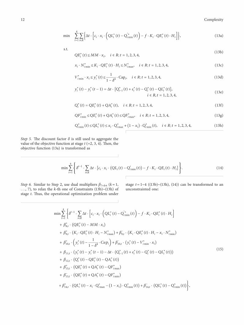
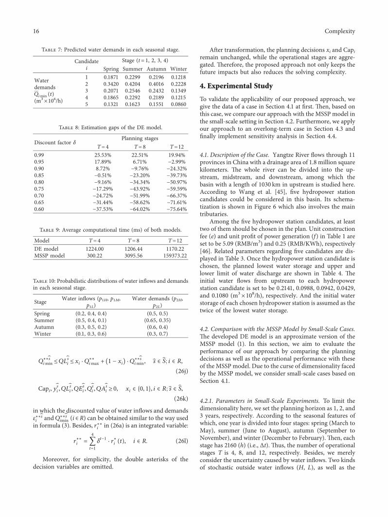
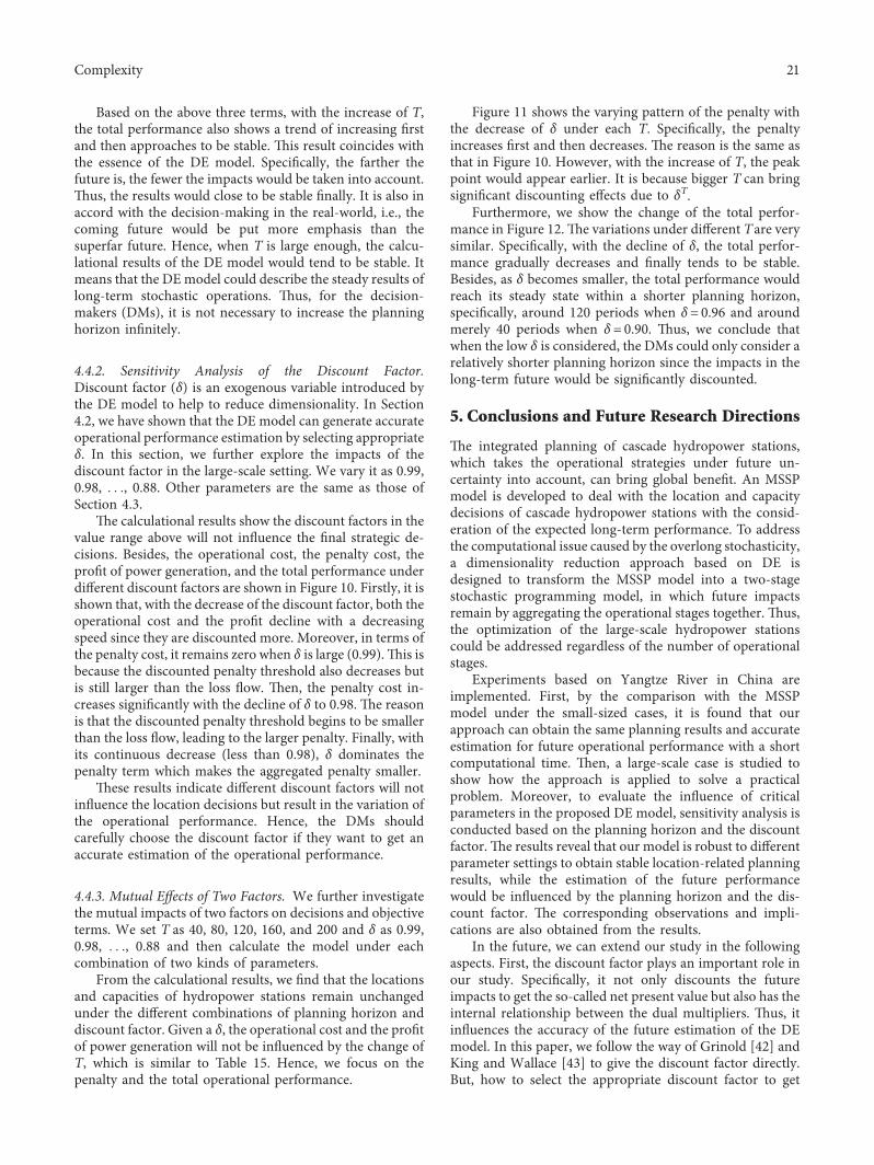