planning as heuristic search -...

Artificial Intelligence 129 (2001) 5–33

Planning as heuristic search

Blai Bonet ∗, Héctor GeffnerDepto. de Computación, Universidad Simón Bolívar, Aptdo. 89000, Caracas 1080-A, Venezuela

Received 15 February 2000

Abstract

In the AIPS98 Planning Contest, the HSP planner showed that heuristic search planners can becompetitive with state-of-the-art Graphplan and SAT planners. Heuristic search planners like HSP

transform planning problems into problems of heuristic search by automatically extracting heuristicsfrom Strips encodings. They differ from specialized problem solvers such as those developed for the24-Puzzle and Rubik’s Cube in that they use a general declarative language for stating problems anda general mechanism for extracting heuristics from these representations.

In this paper, we study a family of heuristic search planners that are based on a simple and generalheuristic that assumes that action preconditions are independent. The heuristic is then used in thecontext of best-first and hill-climbing search algorithms, and is tested over a large collection ofdomains. We then consider variations and extensions such as reversing the direction of the searchfor speeding node evaluation, and extracting information about propositional invariants for avoidingdead-ends. We analyze the resulting planners, evaluate their performance, and explain when theydo best. We also compare the performance of these planners with two state-of-the-art planners, andshow that the simplest planner based on a pure best-first search yields the most solid performanceover a large set of problems. We also discuss the strengths and limitations of this approach, establish acorrespondence between heuristic search planning and Graphplan, and briefly survey recent ideas thatcan reduce the current gap in performance between general heuristic search planners and specializedsolvers. 2001 Elsevier Science B.V. All rights reserved.

Keywords:Planning; Strips; Heuristic search; Domain-independent heuristics; Forward/backward search;Non-optimal planning; Graphplan

1. Introduction

The last few years have seen a number of promising new approaches in Planning.Most prominent among these are Graphplan [3] and Satplan [24]. Both work in stages

* Corresponding author.E-mail addresses:[email protected] (B. Bonet), [email protected] (H. Geffner).

0004-3702/01/$ – see front matter 2001 Elsevier Science B.V. All rights reserved.PII: S0004-3702(01)0 01 08 -4

6 B. Bonet, H. Geffner / Artificial Intelligence 129 (2001) 5–33

by building suitable structures and then searching them for solutions. In Graphplan,the structure is a graph, while in Satplan, it is a set of clauses. Both planners haveshown impressive performance and have attracted a good deal of attention. Recentimplementations and significant extensions have been reported in [2,19,25,27].

In the recent AIPS98 Planning Competition [34], three out of the four planners in theStrips track, IPP [19], STAN [27], and BLACKBOX [25], were based on these ideas. Thefourth planner, HSP [4], was based on the ideas of heuristic search [35,39]. In HSP, thesearch is assumed to be similar to the search in problems like the 8-Puzzle, the maindifference being in the heuristic: while in problems like the 8-Puzzle the heuristic isnormally given (e.g., as the sum of Manhattan distances), in planning it has to be extractedautomatically from the declarative representation of the problem. HSP thus appeals to asimple scheme for computing the heuristic from Strips encodings and uses the heuristic toguide the search for the goal.

The idea of extracting heuristics from declarative problem representations for guidingthe search in planning has been advanced recently by Drew McDermott [31,33], and byBonet, Loerincs and Geffner [6]. 1 In this paper, we extend these ideas, test them overa large number of problems and domains, and introduce a family of planners that arecompetitive with some of the best current planners.

Planners based on the ideas of heuristic search are related to specialized solvers suchas those developed for domains like the 24-Puzzle [26], Rubik’s Cube [23], and Sokoban[17] but differ from them mainly in the use of a general language for stating problems anda general mechanism for extracting heuristics. Heuristic search planners, like all planners,are general problem solversin which the same code must be able to process problems fromdifferent domains [37]. This generality comes normally at a price: as noted in [17], theperformance of the best current planners is still well behind the performance of specializedsolvers. Closing this gap, however, is the main challenge in planning research where theultimate goal is to have systems that combine flexibility and efficiency: flexibility formodeling a wide range of problems, and efficiency for obtaining good solutions fast. 2

In heuristic search planning, this challenge can only be met by the formulation, analysis,and evaluation of suitable domain-independent heuristics and optimizations. In this paperwe aim to present the basic ideas and results we have obtained, and discuss more recentideas that we find promising. 3

More precisely, we will present a family of heuristic search planners based on a simpleand general heuristic that assumes that action preconditions are independent. This heuristicis then used in the context of best-first and hill-climbing search algorithms, and is testedover a large class of domains. We also consider variations and extensions, such as reversingthe direction of the search for speeding node evaluation, and extracting information aboutpropositional invariants for avoiding dead-ends. We compare the resulting planners with

1 This idea also appears, in a different form, in the planner IxTex; see [29].2 Interestingly, the area of constraint programming has similar goals although it is focused on a different class

of problems [16]. Yet, see [45] for a recent attempt to apply the ideas of constraint programming in planning.3 Another way to reduce the gap between planners and specialized solvers is by making room in planning

languages for expressing domain-dependent control knowledge (e.g., [5]). In this paper, however, we don’tconsider this option which is perfectly compatible and complementary with the ideas that we discuss.

B. Bonet, H. Geffner / Artificial Intelligence 129 (2001) 5–33 7

some of the best current planners and show that the simplest planner based on a pure best-first search, yields the most solid performance over a large set of problems. We also discussthe strengths and limitations of this approach, establish a correspondence between heuristicsearch planning and Graphplan, and briefly survey recent ideas that can help reduce theperformance gap between general heuristic search planners and specialized solvers.

Our focus is on non-optimal sequential planning.This is contrast with the recentemphasis on optimal parallel planningfollowing Graphplan and SAT-based planners [24].Algorithms are evaluated in terms of the problems that they solve (given limited time andmemory resources), and the quality of the solutions found (measured by the solution timeand length). The use of heuristics for optimalsequential and parallel planning is consideredin [13] and is briefly discussed in Section 8.

In this paper we review and extend the ideas and results reported in [4]. However, ratherthan focusing on the two specific planners HSP and HSPr, we consider and analyze abroader space of alternatives and perform a more exhaustive empirical evaluation. Thismore systematic study led us to revise some of the conjectures in [4] and to understandbetter the strengths and limitations involved in the choice of the heuristics, the searchalgorithms, and the direction of the search.

The rest of the paper is organized as follows. We cover first general state models(Section 2) and the state models underlying problems expressed in Strips (Section 3). Wethen present a domain-independent heuristic that can be obtained from Strips encodings(Section 4), and use this heuristic in the context of forward and backward state planners(Sections 5 and 6). We then consider related work (Section 7), summarize the main ideasand results, and discuss current open problems (Section 8).

2. State models

State spaces provide the basic action model for problems involving deterministic actionsand complete information. A state spaceconsists of a finite set of states S, a finite setof actions A, a state transition function f that describes how actions map one state intoanother, and a cost function c(a, s) > 0 that measures the cost of doing action a in states [35,38]. A state space extended with a given initial state s0 and a set SG of goal stateswill be called a state model.State models are thus the models underlying most of theproblems considered in heuristic search [39] as well as the problems that fall into the scopeof classical planning [35]. Formally, a state model is a tuple S = 〈S, s0, SG,A,f, c〉 where

• S is a finite and non-empty set of states s,• s0 ∈ S is the initial state,• SG ⊆ S is a non-empty set of goal states,• A(s)⊆A denotes the actions applicable in each state s ∈ S,• f (a, s) denotes a state transition function for all s ∈ S and a ∈A(s), and• c(a, s) stands for the cost of doing action a in state s.

A solutionof a state model is a sequence of actions a0, a1, . . . , an that generates a statetrajectory s0, s1 = f (s0), . . . , sn+1 = f (an, sn) such that each action ai is applicable in siand sn+1 is a goal state, i.e., ai ∈ A(si) and sn+1 ∈ SG. The solution is optimalwhen thetotal cost

∑ni=0 c(ai, si ) is minimized.


In problem solving, it is common to build state models adapted to the target domainby explicitly defining the state space and explicitly coding the state transition functionf (a, s) and the action applicability conditions A(s) in a suitable programming language.In planning, state models are defined implicitly in a general declarative language thatcan easily accommodate representations of different problems. We consider next the statemodels underlying problems expressed in the Strips language [9]. 4

3. The Strips state model

A planning problem in Strips is represented by a tuple P = 〈A,O, I,G〉 where A isa set of atoms, O is a set of operators, and I ⊆ A and G ⊆ A encode the initial and goalsituations. The operators op∈O are all assumed grounded (i.e., with the variables replacedby constants). Each operator has a precondition, add, and delete lists denoted as Prec(op),Add(op), and Del(op) respectively. They are all given by sets of atoms from A. A Stripsproblem P = 〈A,O, I,G〉 defines a state space SP = 〈S, s0, SG,A(·), f, c〉 where

(S1) the states s ∈ S are collections of atoms from A;(S2) the initial state s0 is I ;(S3) the goal states s ∈ SG are such that G⊆ s;(S4) the actions a ∈A(s) are the operators op∈O such that Prec(op)⊆ s;(S5) the transition function f maps states s into states s′ = s − Del(a)+ Add(a) for

a ∈A(s);(S6) all action costs c(a, s) are 1.

The (optimal) solutions of the problem P are the (optimal) solutions of the state modelSP . A possible way to find such solutions is by performing a search in such space. Thisapproach, however, has not been popular in planning where approaches based on divide-and-conquer ideas and search in the space of plans have been more common [35,46].This situation however has changed in the last few years, after Graphplan [3] and SAT

approaches [24] achieved orders of magnitude speed ups over previous approaches. Morerecently, the idea of planning as state space search has been advanced in [31] and [6]. Inboth cases, the key ingredient is the heuristic used to guide the search that is extractedautomatically from the problem representation. Here we follow the formulation in [6].

4. Heuristics

The heuristic function h for solving a problem P in [6] is obtained by considering a‘relaxed’ problem P ′ in which all delete listsare ignored. From any state s, the optimalcost h′(s) for solving the relaxed problem P ′ can be shown to be a lower bound on theoptimal cost h∗(s) for solving the original problem P . As a result, the function h′(s) couldbe used as an admissible heuristic for solving the original problem P . However, solving the‘relaxed’ problem P ′ and obtaining the function h′ are NP-hard problems. 5 We thus use an

4 As it is common, we use the current version of the Strips language as defined by the Strips subset of PDDL

[32] rather than original version in [9].5 This can be shown by reducing set-covering to Strips with no deletes.


approximation and set h(s) to an estimateof the optimal value function h′(s) of the relaxedproblem. In this approximation, we estimate the cost of achieving the goal atoms from s

and then set h′(s) to a suitable combination of those estimates. The cost of individual atomsis computed by a procedure which is similar to the ones used for computing shortest pathsin graphs [1]. Indeed, the initial state and the actions can be understood as defining a graphin atom space in which for every action op there is a directed link from the preconditionsof op to its positive effects. The cost of achieving an atom p is then reflected in the lengthof the paths that lead to p from the initial state. This intuition is formalized below.

We will denote the cost of achieving an atom p from the state s as gs(p). These estimatescan be defined recursively as 6

gs(p)={

0 if p ∈ s,min

op∈O(p)[1 + gs(Prec(op))] otherwise, (1)

whereO(p) stands for the actions op that add p, i.e., with p ∈ Add(op), and gs(Prec(op)),to be defined below, stands for the estimated cost of achieving the preconditions of actionop from s.

While there are many algorithms for obtaining the function gs defined by (1), we usea simple forward chaining procedure in which the measures gs(p) are initialized to 0 ifp ∈ s and to ∞ otherwise. Then, every time an operator op is applicable in s, each atomp ∈ Add(op) is added to s and gs(p) is updated to

gs(p) := min[gs(p), 1 + gs

(Prec(op)

)]. (2)

These updates continue until the measures gs(p) do not change. It’s simple to show thatthe resulting measures satisfy Eq. (1). The procedure is polynomial in the number of atomsand actions, and corresponds essentially to a version of the Bellman–Ford algorithm forfinding shortest paths in graphs [1].

The expression gs(Prec(op)) in both (1) and (2) stands for the estimated cost of the setof atoms given by the preconditions of action op. In planners such as HSP, the cost gs(C) ofa set of atomsC is defined in terms of the cost of the atoms in the set. As we will see below,this can be done in different ways. In any case, the resulting heuristic h(s) that estimatesthe cost of achieving the goalG from a state s is defined as

h(s)def= gs(G). (3)

The cost gs(C) of setsof atoms can be defined as the weighted sum of costs of individualatoms, the minimum of the costs, the maximum of the costs, etc. We consider two ways.The first is as the sumof the costs of the individual atoms in C:

g+s (C)=

∑r∈Cgs(r) (additive costs). (4)

We call the heuristic that results from setting the costs gs(C) to g+s (C), the additive

heuristicand denote it by hadd. The heuristic hadd assumes that subgoals are independent.This is not true in general as the achievement of some subgoals can make the achievement

6 Where the min of an empty set is defined to be infinite.


of the other subgoals more or less difficult. For this reason, the additive heuristic is notadmissible(i.e., it may overestimate the true costs). Still, we will see that it is quite usefulin planning.

Second, an admissible heuristic can be defined by combining the cost of atoms by themaxoperation as:

gmaxs (C)= max

r∈C gs(r) (max costs). (5)

We call the heuristic that results from setting the costs gs(C) to gmaxs (C), the max heuristic

and denote it by hmax. The max heuristic unlike the additive heuristic is admissible as thecost of achieving a set of atoms cannot be lower than the cost of achieving each of theatoms in the set. On the other hand, the max heuristic is often less informative. In fact,while the additive heuristic combines the costs of all subgoals, the max heuristic focusesonly on the most difficult subgoals ignoring all others. In Section 7, however, we will seethat a refined version of the max heuristic is used in Graphplan.

5. Forward state planning

5.1. HSP: A hill-climbing planner

The planner HSP [4] that was entered into the AIPS98 Planning Contest, uses the additiveheuristic hadd to guide a hill-climbing search from the initial state to the goal. The hill-climbing search is very simple: at every step, one of the best children is selected forexpansion and the same process is repeated until the goal is reached. Ties are brokenrandomly. The best children of a node are the ones that minimize the heuristic hadd. Thus,in every step, the estimated atom costs gs(p) and the heuristic h(s) are computed for thestates s that are generated. In HSP, the hill climbing search is extended in several ways; inparticular, the number of consecutive plateau moves in which the value of the heuristic hadd

is not decremented is counted and the search is terminated and restarted when this numberexceeds a given threshold. In addition, all states that have been generated are stored in afast memory (a hash table) so that states that have been already visited are avoided in thesearch and their heuristic values do not have to be recomputed. Also, a simple scheme forrestarting the search from different states is used for avoiding getting trapped into the sameplateaus.

Many of the design choices in HSP are ad-hoc. They were motivated by the goal ofgetting a better performance for the Planning Contest and by our earlier work on a real-time planner based on the same heuristic [6]. HSP did well in the Contest competing in the“Strips track” against three state-of-the-art Graphplan and SAT planners: IPP [19], STAN

[27] and BLACKBOX [25]. Table 1 from [34] shows a summary of the results. In the contestthere were two rounds with 140 and 15 problems each, in both cases drawn from severaldomains. The table shows for each planner in each round, the number of problems solved,the average time taken over the problems that were solved, and the number of problems inwhich each planner was fastest or produced shortest solutions. IPP, STAN and BLACKBOX,are optimal parallel planners that minimize the number of time steps (in which severalactions can be performed concurrently) but not the number of actions.


Table 1Results of the AIPS98 Contest (Strips track). Columns show the number of problemssolved by each planner, the average time over the problems solved (in seconds) andthe number of problems in which each planner was fastest or produced shortest plans(from [34])

Round Planner Avg. time Solved Fastest Shortest

Round 1 BLACKBOX 1.49 63 16 55

HSP 35.48 82 19 61

IPP 7.40 63 29 49

STAN 55.41 64 24 47

Round 2 BLACKBOX 2.46 8 3 6

HSP 25.87 9 1 5

IPP 17.37 11 3 8

STAN 1.33 7 5 4

As it can be seen from the table, HSP solved more problems than the other planners butit often took more time or produced longer plans. More details about the setting and resultsof the competition can be found in [34] and in an article to appear in the AI Magazine.

5.2. HSP2: A best-first search planner

The results above and a number of additional experiments suggest that HSP iscompetitive with the best current planners over many domains. However, HSP is not anoptimal planner, and what’s worse—considering that optimality has not been a traditionalconcern in planning—the search algorithm in HSP is not complete. In this section, weshow that this last problem can be overcome by switching from hill-climbing to a best-firstsearch(BFS) [39]. Moreover, the resulting BFS planner is superior in performance to HSP,and it appears to be superior to some of the best planners over a large class of problems.By performance we mean: the number of problems solved, the time to get those solutions,and the length of those solutions measured by the number of actions.

We will refer to the planner that results from the use of the additive heuristic hadd in abest-first search from the initial state to the goal, as HSP2. This best-first search keeps anOpen and a Closed list of nodes as A∗ [35,39] but weights nodes by an evaluation functionf (n) = g(n) +W · h(n), where g(n) is the accumulated cost, h(n) is the estimated costto the goal, and W � 1 is a constant. For W = 1, the algorithm is A∗ and for W �= 1 itcorresponds to the so-called WA∗ algorithm [39]. Higher values of W usually lead to thegoal faster but with solutions of lower quality [22]. Indeed, if the heuristic is admissible,the solutions found by WA∗ are guaranteed not to exceed the optimal costs by more than afactor ofW . HSP2 uses the WA∗ algorithm with the non-admissible heuristic hadd which isevaluated from scratch in every new state generated. The value of the parameterW is fixedat 5, even though values in the range [2,10] do not make a significant difference.


5.3. Experiments

In the experiments below, we assess the performance of the two heuristic searchplanners, HSP and HSP2, in comparison with two state-of-the-art planners, STAN 3.0 [27],and BLACKBOX 3.6 [25]. HSP and HSP2 both perform a forward state space search guidedby the additive heuristic hadd. The first performs an extended hill-climbing search andthe later performs a best-first search with an evaluation function in which the heuristic ismultiplied by the constantW = 5. STAN and BLACKBOX are both based on Graphplan [3],but the latter maps the plan graph into a set of clauses that are checked for satisfiability.The version of HSP used in the experiments, HSP 1.2, improves the version used in theAIPS98 Contest and the one used in [4].

For each planner and each planning problem we evaluate whether the planner solvesthe problem, and if so, the time taken by the planner and the number of actions in thesolution. STAN and BLACKBOX are optimal parallel planners that minimize the number oftime steps but not necessarily the number of actions. Both planners were run with theirdefault options.

The experiments were performed on an Ultra-5 with 128 Mb RAM and 2 Mb of Cacherunning Solaris 7 at 333 MHz. The exception are the results for BLACKBOX on theLogistics problems that were taken from the BLACKBOX distribution as the default optionsproduced much poorer results. 7 The domains considered are: Blocks, Logistics, Gripper,8-Puzzle, Hanoi, and Tire-World. They constitute a representative sample of difficult butsolvable instances for current planners. Five of the 10 Blocks-World instances are of ourown [4], the rest of the problems are taken from others as noted. A planner is said notto solve a problem when it either runs out of memory or runs out of time (10 minutes).Failure to find solutions due either to memory or time constraints are displayed as planswith length −1.

All the planners are implemented in C and accept problems in the PDDL language (thestandard language used in the AIPS98 Contest; [32]). Moreover, the planners in the HSP

family convert every problem instance in PDDL into a program in C. Generating, compiling,linking, and loading such program takes in the order of 2 seconds. This time is roughlyconstant for all instances and domains, and is not included in the figures below.

5.3.1. Blocks-WorldThe first experiments deal with the blocks world. The blocks world is challenging

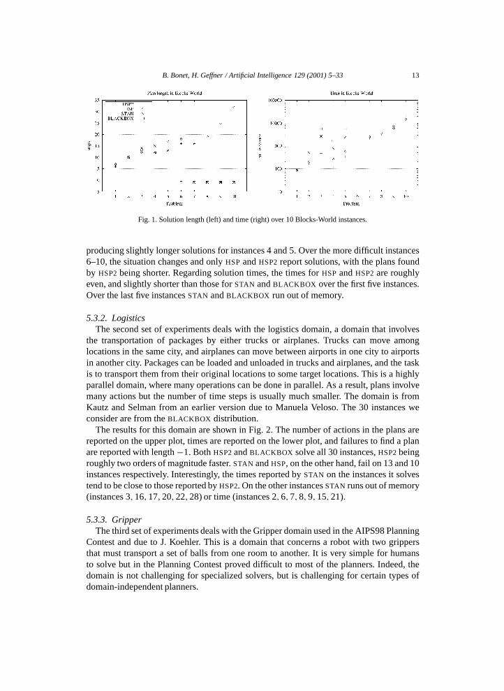
for domain-independent planners due to the interactions among subgoals and the size ofthe state space. The ten instances considered involve from 7 to 19 blocks. Five of theseinstances are taken from the BLACKBOX distribution and five are from [4]. The results forthis domain are shown in Fig. 1 that displays for each planner the lengthof the solutionson the left, and the timeto get those solutions on the right.

The lengths produced by STAN and BLACKBOX are not necessarily optimal in thisdomain as there is some parallelism (e.g., moving blocks among disjoint pairs of towers).This is the reason the lengths they report do not always coincide. In any case, the solutionsreported by the four planners are roughly equivalent over instances 1–5, with STAN and HSP

7 Those results were obtained on a SPARC Ultra 2 with a 296 MHz clock and 256 M of RAM [5].


Fig. 1. Solution length (left) and time (right) over 10 Blocks-World instances.

producing slightly longer solutions for instances 4 and 5. Over the more difficult instances6–10, the situation changes and only HSP and HSP2 report solutions, with the plans foundby HSP2 being shorter. Regarding solution times, the times for HSP and HSP2 are roughlyeven, and slightly shorter than those for STAN and BLACKBOX over the first five instances.Over the last five instances STAN and BLACKBOX run out of memory.

5.3.2. LogisticsThe second set of experiments deals with the logistics domain, a domain that involves

the transportation of packages by either trucks or airplanes. Trucks can move amonglocations in the same city, and airplanes can move between airports in one city to airportsin another city. Packages can be loaded and unloaded in trucks and airplanes, and the taskis to transport them from their original locations to some target locations. This is a highlyparallel domain, where many operations can be done in parallel. As a result, plans involvemany actions but the number of time steps is usually much smaller. The domain is fromKautz and Selman from an earlier version due to Manuela Veloso. The 30 instances weconsider are from the BLACKBOX distribution.

The results for this domain are shown in Fig. 2. The number of actions in the plans arereported on the upper plot, times are reported on the lower plot, and failures to find a planare reported with length −1. Both HSP2 and BLACKBOX solve all 30 instances, HSP2 beingroughly two orders of magnitude faster. STAN and HSP, on the other hand, fail on 13 and 10instances respectively. Interestingly, the times reported by STAN on the instances it solvestend to be close to those reported by HSP2. On the other instances STAN runs out of memory(instances 3,16,17,20,22,28) or time (instances 2,6,7,8,9,15,21).

5.3.3. GripperThe third set of experiments deals with the Gripper domain used in the AIPS98 Planning

Contest and due to J. Koehler. This is a domain that concerns a robot with two grippersthat must transport a set of balls from one room to another. It is very simple for humansto solve but in the Planning Contest proved difficult to most of the planners. Indeed, thedomain is not challenging for specialized solvers, but is challenging for certain types ofdomain-independent planners.


Fig. 2. Solution length (upper) and time (lower) over 30 Logistics instances from Kautz and Selman.

Fig. 3. Solution length (left) and time (right) over 10 Gripper instances from AIPS98 Contest.

The results over 10 Gripper instances from the AIPS98 Contest are shown in Fig. 3.The planners HSP and HSP2 have no difficulties and compute plans with similar lengths.On the other hand, BLACKBOX solves the first two instances only, and STAN the first fourinstances. As shown on the right, the time required by both planners grows exponentiallyand they run out of time over the larger instances. On the other hand, HSP and HSP2 scaleup smoothly with HSP2 being slightly faster than HSP.


One of the reasons for the failure of both STAN and BLACKBOX in Gripper is that theheuristic implicitly represented by the plan graph is a very poor estimator in this domain.As a result, Graphplan-based planners, such as STAN and BLACKBOX that perform a formof IDA∗ search must do many iterations before finding a solution. Actually, the sameexponential growth in Gripper occurs also in HSP planners when the heuristic hmax is usedin place of the additive heuristic. As before, the problem is that the hmax heuristic is almostuseless in this domain where subgoals are mostly independent. The heuristic implicit inthe plan graph is a refinement of the hmax heuristic; the relation between Graphplan andheuristic search planning will be analyzed further in Section 7.

5.3.4. PuzzleThe next problems are four instances of the familiar 8-Puzzle and two instances from the

larger 15-Puzzle. Three of the four 8-Puzzle instances are hard as their optimal solutionsinvolves 31 steps, the maximum plan length in such domain. The 15-Puzzle instances areof medium difficulty.

As shown in Fig. 4, HSP and STAN solve the first four instances, and HSP2 solves the firstfive. The solutions computed by STAN are optimal in this domain which is purely serial.The solutions computed by HSP and HSP2, on the other hand, are poorer, and are often twiceas long. On the other hand, as shown on the left part of the figure, HSP2 is two orders ofmagnitude faster than STAN over the difficult 8-Puzzle instances (2–4) and can also solveinstance 5. The times for HSP are worse and does not solve instance 5. BLACKBOX doesnot solve any of the instances.

5.3.5. HanoiFig. 5 shows the results for Hanoi. Instance i has i + 2 disks, thus problems range from

3 disks up to 8 disks. Over all these problems HSP2 and STAN generate plans of the samequality, HSP2 being slightly faster than STAN. HSP also solves all instances but the solutionsare longer. BLACKBOX solves the first two instances.

Fig. 4. Solution length (left) and time (right) over four instances of the 8-Puzzle (1–4) and two instances of the15-Puzzle (5–6).


Fig. 5. Solution length (left) and time (right) over six Hanoi instances. Instance i has i + 2 disks.

Fig. 6. Solution length (left) and time (right) over three instances of Tire-World.

5.3.6. Tire-WorldThe Tire-World domain is due to S. Russell and involves operations for fixing flat tires:

opening and closing the trunk of a car, fetching and putting away tools, loosening andtightening nuts, etc. Fig. 6 shows the results. Here both STAN and BLACKBOX solve allthree instances producing optimal plans. HSP and HSP2 also solve these instances but insome cases they produce inferior solutions. On the time scale, HSP2 is slightly faster thanSTAN, and both are faster than BLACKBOX in one case by two orders of magnitude. Asbefore, HSP is slower than HSP2 and produces longer solutions.

5.4. Summary: Forward state planning

The experiments above, based on a representative sample of problems, show that the twoforward heuristic search planners HSP and HSP2 are capable of solving the problems solvedby two state-of-the-art planners. In addition, in some domains, HSP and in particular HSP2

solve problems that the other planners with their default settings do not currently solve.The planner HSP2, based on a standard best first search, tends to be faster and more robustthan the hill-climbing HSP planner. Thus, the arguments in [4] in support of a hill-climbingstrategy based on the slow node generation rate that results from the computation of the


heuristic in every state do not appear to hold in general. Indeed, the combination of theadditive heuristic hadd and the multiplying constantW > 1 often drive the best-first plannerto the goal with as few node evaluations as the hill-climbing planner, already providing thenecessary ‘greedy’ bias. An A∗ search with an admissible and consistent heuristic, on theother hand, is bound to expand all nodes n whose cost f (n) is below the optimal cost. Thishowever does no apply to the WA∗ strategy used in HSP2.

In the experiments theW parameter in HSP2 was set to the constant value 5. Yet HSP2 isnot particularly sensitive to the exact value of this constant. Indeed, in most of the domains,values in the interval [2,10] produce similar results. This is likely due to the fact that theheuristic hadd is not admissible and by itself tends to overestimate the true costs withoutthe need of a multiplying factor. On the other hand, in some domains like Logistics andGripper, the value W = 1 does not lead to solutions. This is precisely because in thesedomains that involve subgoals that are mostly independent, the additive heuristic is not‘sufficiently’ overestimating. Finally, in problems like the sliding tile puzzles, values ofW closer to 1 produce better solutions in more time, in correspondence with the normalpattern observed in cases in which the heuristic is admissible [22].

Fig. 7 shows the effects of three different values of W on the quality and times of thesolutions, and the number of nodes generated. The values considered are W = 1, W = 2,andW = 5. The top three curves that correspond to Hanoi, are typical for most of the other

Fig. 7. Influence of value of W in the HSP2 planner on the length of the solutions (left), the time required to findsolutions (center), and number of nodes generated (right). The domains from top to bottom are Hanoi, Gripper,and Puzzle.


domains and show little effect. The second set of curves corresponds to Gripper whereHSP2 fails to solve the last six instances forW = 1. Indeed, the two right most curves showan exponential growth in time and the number of generated nodes. In Logistics, HSP2 withW = 1 also fails to solve most of the instances. As noted above, these are two domainswhere subgoals are mostly independent and where the additive heuristic is not sufficientlyoverestimating and hence fails to provide the ‘greedy bias’ necessary to find the solutions.Indeed, the state space in Logistics is very large, while in Gripper it’s the branching factorthat is large due to the (undetected) symmetries in the problem.

The bottom set of curves in Fig. 7 correspond to the Puzzle domain. In this domain,HSP2 with W = 1 and W = 2 produce better solutions and in some cases take more time.This probably happens in Puzzle because, as in Gripper and Logistics, there is a degree ofdecomposability in the domain (that’s why the sum of the Manhattan distance works), thatmakes the additive heuristic behave as an admissible heuristic in WA∗. Unlike Gripper andLogistic, however the branching factor of the problem and the size of the state space allowthe resulting BFS algorithm to solve the instances even with W = 1. Actually, with W = 1andW = 2, HSP2 solves the sixth instance of Puzzle which is not solved with W = 5.

6. HSPr: Heuristic regression planning

A main bottleneck in both HSP and HSP2 is the computation of the heuristic from scratchin every new state. 8 This takes more than 80% of the total time in both planners and makesthe node generation rate very low. Indeed, in a problem like the 15-Puzzle, both plannersgenerate less than a thousand nodes per second, while a specialized solver such as [26]generates several hundred thousand nodes per second for the more complex 24-Puzzle.The reason for the low node generation rate is the computation of the heuristic in whichthe estimated costs gs(p) for all atoms p are computed from scratch in every new state s.

In [4], we noted that this problem could by solved by performing the search backwardfrom the goal rather than forward from the initial state. In that case, the estimated costsgs0(p) derived for all atoms from the initial state could be used without recomputationfordefining the heuristic of any state s arising in the backward search. Indeed, the estimateddistance from s to s0 is equal to the distance from s0 to s, and this distance can beestimated simply as the sum (or max) of the costs gs0(p) for the atoms p in s. This trickfor simplifying the computation of the heuristic and speeding up node generation resultsfrom computing the estimated atom costs from a state s0 which then becomes the targetof the search. An alternative is to estimate the atom costs from the goal and then performa forward search toward the goal. This is actually the idea in [43]. The problem with thislatter scheme is that the goal in planning is not a state but a set of states;namely, the stateswhere the goal atoms hold. And computing the heuristic from a set of states in a principledmanner is bound to be more difficult than computing the heuristic from a given state (thusthe need to ‘complete’ the goal description in [43]).

We thus present below a scheme for performing planning as heuristic search that avoidsthe recomputation of the atom costs in every new state by computing these costs oncefrom

8 The same applies also to McDermott’s UNPOP.


the initial state s0. These costs are then used without recomputationto define an heuristicthat is used to guide a regressionsearch from the goal. The benefit of the search scheme isthat node generation will be 6–7 times faster. This will show in the solution of some of theproblems considered above such as Logistics and Gripper. However, as we will also see,in many problems the new search scheme does not help, and in several cases, it actuallyhurts. We discuss such issues below.

6.1. Regression state space

We refer to the planner that searches backward from the goal rather than forwardfrom the initial state as HSPr. Backward search is an old idea in planning that is knownas regression search[35,46]. In regression search, the states can be thought as sets ofsubgoals;i.e., the ‘application’ of an action in a goal yields a situation in which theexecution of the action achieves the goal. Moreover, while a set of atoms {p,q, r} in theforward search represents the uniquestate in which the atoms p, q , and r are true andall other atoms are false, the same set of atoms in the regression search represents thecollectionof states in which the atoms p, q , and r are true. In particular, the set of goalsatomsG, which determines the root node of the regression search, stands for the collectionof goal states, that is, the states s such that G⊆ s.

For making precise the nature of the backward search, we will thus define explicitly thestate space being searched. We will call it the regression spaceand define it in analogy tothe progression spaceSP defined by (S1)–(S5) above. The regression space RP associatedwith a Strips problem P = 〈A,O, I,G〉 is given by the tuple RP = 〈S, s0,SG,A(·), f, c〉where

(R1) the states s are sets of atoms from A;(R2) the initial state s0 is the goal G;(R3) the goal states s ∈ SG are the states for which s ⊆ I ;(R4) the set of actions A(s) applicable in s are the operators op∈ O that are relevant

and consistent;namely, for which Add(op)∩ s �= ∅ and Del(op)∩ s = ∅;(R5) the state s′ = f(a, s) that follows the application of a ∈ A(s) is such that s′ =

s − Add(a)+ Prec(a);(R6) the action costs c(a, s) are all 1.

The solution of this state space is, like the solution of any state model 〈S, s0,SG,A(·), f, c〉,a finite sequence of actions a0, a1, . . . , an such that for a sequence of states s0, s1, . . . ,sn+1, si+1 = f(ai, si ), for i = 0, . . . , n, ai ∈ A(si ), and sn+1 ∈ SG. The solution of theprogression and regression spaces are related in the obvious way; one is the inverse of theother.

We use different fonts for referring to states s in the progression space SP and states sin the regression space RP . While they are both represented by sets of atoms, they have adifferent meaning. As we said above, the state s = {p,q, r} in the regression space standsfor the setof states s, {p,q, r} ⊆ s in the progression space. For this reason, forward andbackward search in planning are not symmetric, unlike forward and backward search inproblems like the 15-Puzzle or Rubik’s Cube.


6.2. Heuristic

The planner HSPr searches the regression space (R1)–(R5) using an heuristic based onthe additive cost estimates gs(p) described in Section 4. These estimates are computedonly once from the initial state s0 ∈ S . The heuristic hadd(s) associated with anystate s isthen defined as

hadd(s)=∑p∈s

gs0(p). (6)

While in HSP, the heuristic hadd(s) combines the cost estimates gs(p) of a fixed set ofgoal atoms computed from each state s, in HSPr, the heuristic hadd(s) combines the costestimates of the set of subgoals p in s from a fixed state s0. The heuristic hmax(s) can bedefined in an analogous way by replacing sums by maximizations.

6.3. Mutexes

The regression search often leads to states s that are not reachable from the initial states0. For example, in the Blocks-World, the regression of the state

s = {on(c, d),on(a, b)

}through the action move(a, d, b) leads to the state

s′ = {on(c, d),on(a, d),clear(b),clear(a)

}.

This state represents a situation in which two blocks, c and a are on the same block d .It is simple to show that such situations are unreachable in the Block-Worlds given a‘normal’ initial state. Such unreachable situations are common in regression planning, andif undetected, cause a lot of useless search. A good heuristic would assign an infinite cost tosuch situations but our heuristics are not as good. Indeed, the basic assumption underlyingboth the additive and the max heuristics—that the estimated cost of a set of atoms is afunction of the estimated cost of the atoms in the set—is violated in such situations. Indeed,while the cost of each of the atoms on(c, d) and on(a, d) is finite, the cost of the pair ofatoms {on(c, d),on(a, d)} is infinite. Better heuristics that do not make this assumption andcorrectly reflect the cost of such pairs of atoms have been recently described in [13]. Herewe follow [4] and develop a simple mechanism for detecting some pairs of atoms {p,q}such that any state containing those pairs can be proven to be unreachable from the initialstate, and thus can be given an infinite heuristic value and pruned. The idea is adaptedfrom a similar idea used in Graphplan [3] and thus we call such pairs of unreachableatoms mutually exclusive pairs or mutexpairs. As in Graphplan, the definition below isnot guaranteed to identify all mutex pairs, and furthermore, it says nothing about largersets of atoms that are not achievable from s0 but whose proper subsets are.

A tentative definition is to identify a pair of atoms R as a mutex when R is not true in theinitial state s0 and every action that asserts an atom in R deletes the other. This definitionis sound (it only recognizes pairs of atoms that are not achievable jointly) but is too weak.In particular, it does not recognize a set of atoms like {on(a, b),on(a, c)} as a mutex, sinceactions like move(a, d, b) add the first atom but do not delete the second.


We thus use a different definition in which a pair of atoms R is recognized as mutexwhen the actions that add one of the atoms in R and do not delete the other atom, canguarantee through their preconditions that such atom will not be true after the action. Toformalize this, we consider setsof mutexes rather that individual pairs.

Definition 1. A setM of atom pairs is a mutex setgiven a set of operatorsO and an initialstate s0 iff for all atoms pairs R = {p,q} in M

(1) R is not true in s0,(2) for every op∈O that adds p, either opdeletes q , or opdoes not add q and for some

precondition r of op, R′ = {r, q} is a pair in M .

It is simple to verify that if a pair of atoms R belongs to a mutex set, then the atomsin R are really mutually exclusive, i.e., not achievable from the initial state given theavailable operators. Also if M1 and M2 are two mutex sets, M1 ∪M2 will be a mutexset as well, and hence according to this definition, there is a single largest mutex set.Rather than computing this set, however, that is difficult, we compute an approximation asfollows.

We say that a pair R′ is a ‘bad pair’ in M when R′ does not comply with one of theconditions (1)–(2) above. The procedure for constructing a mutex set starts with a set ofpairsM :=M0 and iteratively removes all bad pairs fromM until no bad pair remains. Theinitial set M0 of ‘potential’ mutexes can be chosen in a number of ways. In all cases, theresult of this procedure is a mutex setM such thatM ⊆M0. One possibility is to setM0 tothe set of all pairs of atoms. In [4], to avoid the overhead involved in dealing with the N2/2pairs of atoms and many useless mutexes, we chose a smaller set M0 of potential mutexesthat turns out to be adequate for many domains. Such set M0 was defined as the union ofthe sets MA andMB where

• MA is the set of pairs P = {p,q} such that some action adds p and deletes q ,• MB is the set of pairs P = {r, q} such that for some pair P ′ = {p,q} inMA and some

action a, r ∈ Prec(a) and p ∈ Add(a).The structure of this definition mirrors the structure of the definition of mutex sets.

A mutex in HSPr refers to a pair in the set M∗ obtained from the set M0 =MA +MBby sequentially removing all ‘bad’ pairs. Like the analogous definition in Graphplan, theset M∗ does not capture all actual mutexes, yet it can be computed fast, and in manyof the domains we have considered appears to prune the obvious unreachable states.A difference with Graphplan is that this definition identifies structural mutexeswhileGraphplan identifies time-dependentmutexes. These two sets overlap, but each containspairs the other does not. They are used in different ways in Graphplan and HSPr. Forexample, in the complete TSP domain [27], pairs like 〈at(city1),at(city2)〉 would berecognized as a mutex by this definition but not by Graphplan, as the actions of goingto different cities are not mutually exclusive for Graphplan. 9

9 Yet see [28] for using Graphplan to identify some structural mutexes.


6.4. Algorithm

The planner HSPr uses the additive heuristic hadd and the mutex set M∗ to guide aregression search from the goal. The additive heuristic is obtained from the estimated costsgs0(p) computed once for all atoms p from the initial state s0. The mutex setM∗ is used to‘patch’ the heuristic: states s arising in the search that contain a pair in M∗ get an infinitecost and are pruned. The algorithm used for searching the regression space is the sameas the ones used in HSP2: a WA∗ algorithm with the constant W set to 5. Here we departfrom the description of HSPr in [4] where the WA∗ algorithm was given a ‘greedy’ bias. Asabove, we stick to a pure BFS algorithm. The set of experiments below cover more domainsthan those in [4] and will help us to assess better the strengths and limitations of regressionheuristic planning in relation to forward heuristic planning.

6.5. Experiments

In the experiments, we compare the regression planner HSPr with the forward plannerHSP2. Both are based on a WA∗ search and both use the same additive heuristic (in the caseof HSPr, patched with the mutex information). HSPr avoids the recomputation of the atomcosts in every state, and thus computes the heuristic faster and can explore more nodes inthe same time. As we will see, this helps in some domains. However, in other domains,HSPr is not more powerful than HSP2, and in some domains HSPr is actually weaker.This is due to two reasons: first, the additional information obtained by the recomputationof the atom costs in every state sometimes pays off, and second, the regression searchoften generates spurious states that are not recognized as such by the mutex mechanismand cause a lot of useless search. These problems are not significant in the two domainsconsidered in [4] but are significant in other domains.

6.5.1. LogisticsFig. 8 shows the results of the two planners HSPr and HSP2 over the Logistics instances

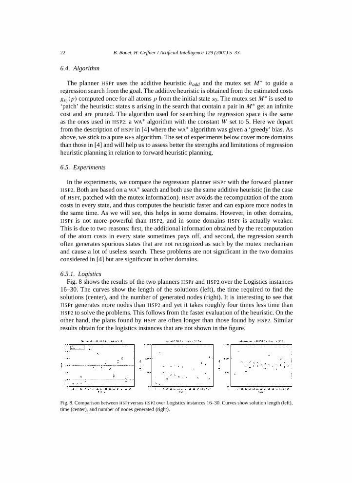
16–30. The curves show the length of the solutions (left), the time required to find thesolutions (center), and the number of generated nodes (right). It is interesting to see thatHSPr generates more nodes than HSP2 and yet it takes roughly four times less time thanHSP2 to solve the problems. This follows from the faster evaluation of the heuristic. On theother hand, the plans found by HSPr are often longer than those found by HSP2. Similarresults obtain for the logistics instances that are not shown in the figure.

Fig. 8. Comparison between HSPr versus HSP2 over Logistics instances 16–30. Curves show solution length (left),time (center), and number of nodes generated (right).


Fig. 9. Comparison between HSPr versus HSP2 over Gripper instances. Curves show solution length (left), solution(center), and number of nodes generated (right).

Fig. 10. Comparison between HSPr versus HSP2 over Hanoi. Curves show solution length (left), solution (center),and number of nodes generated (right). Instance i has i + 2 disks.

6.5.2. GripperAs shown in Fig. 9, a similar pattern arises in Gripper. Here HSPr generates slightly less

nodes than HSP2, but since it generates nodes faster, the time gap between the two plannergets larger as the size of the problems grows. In this case, the solutions found by HSPr areuniformly better than the solutions found by HSP2, and this difference grows with the sizeof the problems.

HSPr is also stronger than HSP2 in Puzzle where, unlike HSP2 (withW = 5), it solves thelast instance in the set (a 15-Puzzle instance). However, for the other three domains HSPrdoes not improve on HSP2, and indeed, in two of these domains (Hanoi and Tire-World) itdoes significatively worse.

6.5.3. Hanoi and Tire-WorldThe results for Hanoi are shown in Fig. 10. HSPr solves the first three instances (up to

5 disks), but it does not solve the other three. Indeed, as it can be seen, in the first threeinstances the time to find the solutions and the number of nodes generated grow muchfaster in HSPr than in HSP2. The same situation arises in the Tire-World where HSP2 solvesall three instances and HSPr solves only the first one. The problems, as we mentionedabove, are two: spurious states generated in the regression search that are not detected bythe mutex mechanisms, and the lack of the ‘feedback’ provided by the recomputation ofthe atom costs in every state. Indeed, errors in the estimated costs of atoms in HSP2 can becorrected when they are recomputed; in HSPr, on the other hand, they are never recomputed.So the recomputation of these costs has two effects, one that is bad (time overhead) andone that is good (additional information). In domains where subgoals interact in complexways, the idea of a forward search in which atom costs are recomputed in every state as


implemented in HSP2 will probably make sense; on the other hand, in domains where theadditive heuristic is adequate, the backward search with no recomputations as implementedin HSPr can be more efficient.

The results for the HSPr and HSP2 planners in the Tire-World show the same pattern asHanoi. Indeed, HSPr solves just the first instance, while HSP2 solves the three instances. Aswe show below, however, part of the problem in this domain has to do with the spuriousstates generated in the regression search.

6.6. Improved mutex computation

The procedure used in HSPr to identify mutexes starts with a setM0 of potential mutexesand then removes the ‘bad’ pairs fromM0 until no ‘bad’ pair remains. A problem we havedetected with the definition in [4], which we have used here, is that the set of potentialmutexesM0 sometimes is not large enough and hence useful mutexes are lost. Indeed, weperformed experiments in whichM0 is set to the collection of all atom pairs, and the sameprocedure is applied to this set until no ‘bad’ pairs remains. In most of the domains, thischange didn’t yield a different behavior. However, there were two exceptions. While HSPrsolved only the first instance of the Tire-World, HSPr using the extended set of potentialmutexes solved the three instances. This shows that in this case HSPr was affected by theproblem of spurious states. On the other hand, in problems like logistics, the new set M0leads to a much larger set of mutexesM∗ that are not as useful and yet have to be checkedin all the states generated. This slows down node generation with no compensating gainthus making HSPr several times slower. The corresponding curves are shown in Fig. 11,where ‘mutex-1’ and ‘mutex-2’ correspond to the original and extended definition of thesetM0 of potential mutexes. Since, the benefits appear to be more important than the loses,the extended definition seems worthwhile and we will make it the default option in the nextversion of HSPr. However, since for the reasons above, the new mechanism is not complete

Fig. 11. Impact of original versus extended definition of the set M0 of potential mutexes in Tire-World andLogistics.


either, the problem caused by the presence of spurious states in regression planning remainsopen. 10

6.7. Additional issues in heuristic regression planning

6.7.1. Additive versus max heuristicWhile we defined two heuristics, the additive heuristic hadd and the max heuristic hmax,

we have used only the additive heuristic. The intuition underlying this choice is that theadditive heuristic is more informed as it takes into account all subgoals, while the maxheuristic only focuses on the subgoals that are perceived as most costly. In order to test thisintuition we ran HSPr over all the domains with the additive heuristic and the max heuristic.In problems that involve many independent subgoals such as Gripper and Logistics, themax heuristic is almost useless and very few instances are solved. On the other hand, inproblem that involve more complex interactions among goals such as Hanoi and Tire-World, the heuristic hmax does slightly better than hadd, and indeed, in Tire-World it solvesthe second instance that hadd does not solve (within HSPr). Finally in Blocks-World andPuzzle where there is a certain degree of decomposability, the hmax heuristic is worse thanthe hadd heuristic but still manages to solve roughly the same set of instances taking moretime.

In summary, the additive heuristic yields a better behavior in HSPr than the max heuristic,but this does not mean that the max heuristic is useless. The heuristic used implicitly inGraphplan is as a refinement of the hmaxheuristic, as is the family of higher-order heuristicformulated in [13]. We will say more about those heuristics below.

6.7.2. Greedy best-first searchThe algorithm used in the version of the HSPr planner presented in [4] uses the same

WA∗ algorithm but with the following variation: when some of the children of the lastexpanded node improve the heuristic value of the parent, the best such child is selected forexpansion even if such node is not a least cost node in the Open list. The idea is to providean additional greedy bias in the search. This modification helps in some instances and ingeneral does not appear to hurt, yet the boost in performance across a large set of domainsis small. For this reason, we have dropped this feature from HSPr which is now a pure BFS

regression planner.

6.7.3. Branching factorA common argument for performing regression search rather than forward search in

planning has been based on considerations related to the branching factors of the twospaces [35,46]. We have measured the forward and backward branching factor in all thedomains and found that they vary a lot from instance to instance. For example, the forwardbranching factor in the Blocks-World instances ranges from 16.83 to 84.62, while thebackward branching factor ranges from 4.73 to 12.15. In Logistics, the forward branchingfactor ranges from 7.89 to 37.91, while the backward factor ranges from 9.68 to 25.80. In

10 As noted in [3], the problem of detecting all mutexes, and even only all mutex pairs, is as hard as the planexistence problem. For other work addressing the derivation of invariants from planning theories; see [11,42].


problems like Puzzle and Hanoi, the average branching factors are roughly constant overthe different instances, and are similar in both directions.

We have found, however, that the performance of the two planners, HSP2 and HSPr,on the same problem is not in direct correspondence with the size of the forward andbackward branching factors. For example, while for each Blocks-World instance theaverage branching factor in HSPr is less than half the one in HSP2, and moreover the firstplanner generates nodes 6–7 times faster on average than the second, HSPr is not better thanHSP2 in blocks world. On the other hand, in logistics, where the average branching factorin HSP2 is often smaller than the one in HSPr, HSPr does better. Thus while considerationsrelated to the branching factor of the forward and backward spaces are relevant to theperformance of planners, they are not the only or most important consideration. As wementioned, two considerations that are relevant for explaining the performance of HSPrin relation to HSP2 are the quality of the heuristic (which in HSP2 is recomputed in everystate), and the presence of spurious states in the regression search (that do not arise in theforward search). This last problem, however, could be solved by the formulation of betterplanning heuristics in which the cost of a set of atoms is not defined in terms of the costsof the individual atoms in the set as in the hadd and hmax heuristics. Such heuristics areconsidered in [13] and are briefly discussed below.

7. Related work

7.1. Heuristic search planning

The idea of extracting heuristics from declarative problem representations in planninghas been proposed recently by McDermott [31] and by Bonet, Loerincs, and Geffner [6].In [6], the heuristic is used to guide a real-time planner based on the LRTA∗ algorithm[21], while in [31], the heuristic is used to guide a limited discrepancy search [12]. Theheuristics in both cases are similar, even though the formulation and the algorithms usedfor computing them are different. The performance of McDermott’s UNPOP, however, doesnot appear to be competitive with the type of planners discussed in this paper. This may bedue to the fact that it is written in Lisp and deals with variables and matching operationsat run-time. Most current planners, including those reported in this paper, are written in Cand deal with grounded operators only. On the other hand, while most of these planners arerestricted to small variations of the Strips language, UNPOP deals with the more expressiveADL [40].

The idea of performing a regression search from the goal for avoiding the recomputationof the atom costs was presented in [4] where the HSPr planner was introduced. Theversion of HSPr considered here, unlike the version reported in [4], is based on a pureBFS algorithm. Likewise, the pure BFS forward planner that we have called HSP2, hasn’tbeen discussed elsewhere. HSP2 is the simplest, and as the experiments have illustrated, itis also the most solid planner in the HSP family.

Two advantages of forward planners over regression planners is that the former do notgenerate spurious states and they often benefit from the additional information obtainedby the recomputation of the atom costs in every state. Mutex mechanisms such as those


used by HSPr and Graphplan can prune some of spurious states in some problems, but theycannot be complete.

The idea of combining a forward propagation from s0 to compute all atom costs anda backward search from the goal for avoiding the recomputation of these costs appearsin reverse form in [43]. Refanidis and Vlahavas compute cost estimates by a backwardpropagation from the goal and then use those estimates to perform a forward state spacesearch from the initial state. In addition, they compute the heuristic in a different way sothey get more accurate estimates.

7.2. Derivation of heuristics

The non-admissible heuristic hadd used in HSP is derived as an approximationof theoptimal cost function of a relaxedproblem where deletes lists are ignored. This formulationhas two obvious problems. First, the approximationis not very good as it ignores thepositiveinteractions among subgoals that can make one goal simpler after a second one hasbeen achieved (this results in the heuristic being non-admissible). Second, the relaxationis not good as it ignores the negativeinteractions among subgoals that are lost whendelete lists are discarded. These two problems are addressed in the heuristic proposed byRefanidis and Vlahavas [43] but their heuristic is still non-admissible and does not haveclear justification.

A different approach for addressing these limitations has been reported recently in [13].While the idea of the hmaxheuristic presented in Section 4 is to approximate the cost of a setof atoms by the cost of the most costly atom in the set, the idea in [13] is to approximatethe cost of a set of atoms by the cost of the the most costly atom pair in the set. Theresulting heuristic, called h2, is admissible and more informative than the hmax heuristic,and can be computed reasonably fast. Indeed, in [13] the h2 heuristic is used in the contextof an IDA∗ search to compute optimalplans. Higher-order heuristics hm in which the costof sets of atoms is approximated by the most costly subset of size m are also discussed.Such higher-order heuristics may prove useful in problems in which subgoals interact incomplex ways.

The derivation of admissible heuristics by the consideration of relaxed models has a longhistory in AI. Indeed, the Manhattan distance heuristic in sliding tile puzzles is normallyexplained in terms of the solution of a relaxed problem in which tiles can move to anyneighboring position [39]. A similar relaxation is used to explain the Minimum SpanningTree heuristic used for solving the Traveling Salesman Problem. Moreover, in [39], theserelaxations are shown to follow from simplifications in suitable Strips encodings, and inparticular the Manhattan heuristic is derived by ignoring some action preconditions.

The idea of deriving heuristics from suitable relaxations is a powerful idea. However, it isoften too general to provide practical guidance in the formulation of concrete heuristics forspecific problems. Indeed, the idea of dropping action preconditions from Strips encodingsis guaranteed to lead to admissible heuristics but computing such heuristics can be ashard as solving the original problem. Indeed, unless we remove all preconditions theclass of ‘relaxed’ planning problems is still intractable. In this paper, we have used adifferent relaxation in which delete lists are removed. While, the resulting problem is stillintractable, its optimal cost can be approximated by the methods discussed in Section 4.


It would be interesting to see if useful heuristics for planning could be obtained bypolynomial approximations that simplify the preconditions rather than the action deletelists. The scheme for deriving admissible heuristics from [13] can actually be seen fromthis perspective.

The automatic derivations of useful admissible heuristics has also been tackled byPrieditis [41]. Prieditis’ scheme is based on a set of transformations that generate a largespace of relaxations given problems expressed in a version of Strips. This space is thensearched for relaxations that produce heuristics that speed up the search in the originalproblem. He shows that a number of interesting heuristics can be identified in this way. Ourwork departs from this in that we stick to one particular type of relaxation for all problems.However, an scheme like Prieditis’ could be used as an off-line learning component ofheuristic search planners that could tune the type of heuristic for the given domain.

A more recent scheme for deriving heuristics is based on the notion of pattern databasesdeveloped by Culberson and Schaeffer [8] and used by Korf for finding optimal solutionsto Rubik’s Cube [23]. In a problem like the 15-Puzzle, a pattern database can be understoodas a table that contains the optimal costs associated with a relaxed (abstracted) state modelin which the location of a certain set of tiles are ignored. Since the relaxed state model canhave a much smaller size than the original state model, it can be solved optimally by blindsearch (e.g., breadth-first search). Then the heuristic h(s) of a state s can be obtained bytaking the distance from the projection of s to the projection of the goal G in the relaxedstate model. If there are several pattern databases, the maximum of these distances is takeninstead. The idea of pattern databases is powerful but is not completely general. Indeed,the size of the relaxed state model that arises in planning problems when the values ofcertain state-variables are ignored, is not necessarily smaller than the size of the originalproblem ([14] mentions the case of the Blocks-World). However, the idea applies verywell to permutation problems such as sliding tile puzzles and Rubik’s Cube, and may haveapplication in many planning domains.

Korf and Taylor [26] also sketch a theory of heuristics that may have application indomain-independent planning. In the sliding tile puzzles, their idea is to solve a number of‘relaxed’ problems in which we only care about disjoint subsets of tiles and in each casewe only count the moves of the tiles selected. Then the addition of such counts providesan admissible heuristic for the original problem. As in the case of pattern databases, eachof the relaxed problems involves a smaller state model that can be solved by brute-forcemethods. Also as for pattern databases, the approach seems applicable to permutationproblems but not to arbitrary planning problems. In particular, it’s not clear how to applythese ideas to a problem like Blocks-World.

7.3. Heuristic regression planning and Graphplan

The operation of the regression planner HSPr consists of two phases. In the first, aforward propagation is used to estimate the costs of all atoms from the initial state s0, and inthe second, a regression search is performed using those measures. These two phases are incorrespondence with the two operation phases in Graphplan [3] where a plan graph is builtforward in a first phase, and is searched backward for plans in the second. The two plannersare also related in the use of mutexes, and idea that HSPr borrows from Graphplan. For the


rest, HSPr and Graphplan look quite different. However, Graphplan can also be understoodas an heuristic search planner with a precise heuristic function and search algorithm. Fromthis point of view, the main innovation in Graphplan is the implementation of the searchthat takes advantage of the plan graph and is quite efficient, and the derivation of theheuristic that makes use of the mutex information. More precisely, from the perspectiveof heuristic search planning, the main features of Graphplan can be understood as follows:

(1) Plan graph: The plan graph encodes an admissible heuristic hG where hG(s) = jiff j is the index of the first level in the graph that includes s without a mutex and inwhich s is not memoized (memoizations are updates on the heuristic function; see(4). The heuristic hG is a refined version of the hmaxheuristic discussed in Section 4,and is closely related to the family of admissible heuristics formulated in [13]. 11

(2) Mutex: Mutexes are used to prune states in the regression search (as in HSPr) and torefine the heuristic hmax. In particular, the cost of a set of atoms C is no longer givenby the cost of the most costly atom in the set when in the first layer that contains C,C occurs with a mutex.

(3) Algorithm: The search algorithm is a version of Iterative Deepening A∗ (IDA∗) [20],where the sumof the accumulated cost g(n) and the estimated cost hG(n) is used toprune nodes n whose cost exceed the current threshold. Actually Graphplan nevergenerates such nodes. The algorithm takes advantage of the information stored inthe plan graph and converts the search in a ‘solution extraction’ procedure.

(4) Memoization: Memoizations are updates on the heuristic function hG (see (1)). Theresulting algorithm is a memory-extended version of IDA∗ that closely correspondsto the MREC algorithm [44]. In MREC, the heuristic of a node n is updated and storedin a hash-table after the search below the children of n completes without a solution(given the current threshold).

(5) Parallelism: Graphplan, unlike HSPr, searches a parallel regression space. While thebranching factor in this search can be very high, Graphplan makes smart use of theinformation in the graph to generate only the children that are ‘relevant’ and whosecost does not exceed the current threshold. The branching rule used in Graphplan ismade explicit in [13].

In [13] Graphplan is compared with a pure IDA∗ planner based on an admissibleheuristic equivalent to Graphplan’s hG. In sequential domains the planners have a similarperformance, but on parallel domains, Graphplan is more than an order of magnitude fasterdue to the more efficient IDA∗ search afforded by the plan graph. The plan graph, however,restricts Graphplan to IDA∗ searches, and it cannot be easily adapted to best-first searchesor WIDA∗ searches [22] unless one abandons the idea of search as solution extraction; see[18].

8. Conclusions

We have presented a formulation of planning as heuristic search and have shown thatsimple state space search algorithms guided by a general domain-independent heuristic

11 The hG heuristic is extracted from the plan graph and used to guide an explicit search in [36].


produce a family of planners that are competitive with some of the best current planners.We have also explored a number of variations, such as reversing the direction of the searchfor accelerating node evaluation, and extracting information about propositional invariantsfor avoiding dead-ends. The planner that showed the most solid performance, however,was the simplest planner, HSP2, based on a best-first forward search, in which atom costsare recomputed from scratch in every state.

Heuristic search planners are related to specialized problem solvers but differ from themin the use of a general declarative language for stating problems and a general mechanismfor extracting heuristics. Planners must offer good modeling language for expressingproblems in a convenient way, and general solvers for operating on those representationsand producing efficient solutions.

A concrete challenge for the future is to reduce the gap in performance between heuristicsearch planners and specialized problem solvers in domains like the 24-Puzzle [26],Rubik’s Cube [23], and Sokoban [17]. In addition, for planners to be more applicableto real problems, it is necessary that they handle aspects such as non-Boolean variables,action durations, and parallel actions. Planners should be able to accommodate a rich classof scheduling problems, yet very few planners currently have such capabilities, and evenfewer if any can compete with specialized solvers. Three issues that we believe must beaddressed in order to make heuristic search planners more general and more powerful arethe ones discussed below.

• Heuristics: The heuristics hadd and hmax considered in this paper are poor estimators,and cannot compete with specialized heuristics. The heuristic hG used in Graphplanis better than hmax but it is not good enough for problems like Rubik’s Cube or the24-Puzzle where subgoals interact in complex ways. In [13], a class of admissibleheuristics hm are formulated in which the cost of a set of atoms C is approximatedby the cost of the mostly costly subset of size m. For m = 1, hm reduces to thehmax heuristic, and for m = 2, hm reduces to the Graphplan heuristic. Higher-orderheuristics, for m > 2, may prove effective in complex problems such as the 24-Puzzle and Rubik’s Cube, and they may actually be competitive with the specializedheuristics used for those problems [23,26]. As mentioned in [13], the challenge is tocompute such heuristics reasonably fast, and to use them with little overhead at runtime. Such higher-order heuristics are related to pattern databases [8], but they areapplicable to all planning problems and not only to permutation problems.

• Branching rules: In highly parallel domains like Rockets and Logistics, SAT

approaches appear to perform best among optimal parallel planners. This may be dueto the branching scheme used. In SAT formulations, the space is explored by settingthe value of any variable at any time point, and then considering each of the resultingstate partitions separately. In Graphplan and in heuristic search approaches, thesplitting is done by applying all possible actions. Yet alternative branching schemes,are common in heuristic branch-and-bound search procedures [30], in particular, inscheduling applications [7]. Work on parallel planning, in particular involving actionsof different durations, would most likely require such alternative branching schemes.

• Modeling languages: All the planners discussed in this paper are Strips planners. Yetfew real problems can actually be encoded efficiently in Strips. This has motivatedthe development of extensions such as ADL [40] and Functional Strips [10]. From the


point of view of heuristic search planning, the issue becomes the derivation of goodheuristics from such richer languages. The ideas considered in this paper do not carrydirectly to such languages but it seems that it should be possible to exploit the richerrepresentations for extracting better heuristics.

Acknowledgements

We thank Daniel Le Berre, Rina Dechter, Patrik Haslum, Jörg Hoffmann, RaoKambhampati, Richard Korf, and Drew McDermott for discussions related to this work.This work has been partially supported by grant S1-96001365 from Conicit, Venezuelaand by the Wallenberg Foundation, Sweden. Blai Bonet is currently at UCLA with a USB-Conicit fellowship.

Appendix A. Postscript

A few months after finishing this paper, the Second AIPS Planning Competition tookplace. The chair was Fahiem Bacchus, who will report the results in a forthcoming issue ofthe AI Magazine. This time there were two tracks, one for domain-independent planners,the other for hand-tailored systems. HSP2 participated in the first track, along with elevenother planners, including the three other planners that participated the first time: IPP,STAN, and BLACKBOX. In this second competition, half of the planners, i.e., six planners,extracted and used heuristic estimators to guide the search for plans. The top performingplanner was FF [15], an heuristic search planner based on a forward hill-climbing search.HSP2 ended second, along with three other planners. The performance of FF was quiteimpressive solving almost all problems, really fast, producing in most cases very goodsolutions. FF differs from HSP in three ways:

(1) the heuristic, which provides a better approximation of the cost of the relaxedplanning problem without deletes,

(2) the search algorithm, which is a hill-climbing search with a lookahead mechanism,and

(3) the addition of a fast pruning criterion that allows some states to be discardedwithout even computing their heuristic values.

These three modifications, together, seem to combine very well, as Jörg Hoffmann showsin a forthcoming paper.

References

[1] R. Ahuja, T. Magnanti, J. Orlin, Network Flows: Theory, Algorithms, and Applications, Prentice-Hall,Englewood Cliffs, NJ, 1993.

[2] C. Anderson, D. Smith, D. Weld, Conditional effects in Graphplan, in: Proc. 4th International Conferenceon AI Planning Systems, AAAI Press, Menlo Park, CA, 1998, pp. 44–53.

[3] A. Blum, M. Furst, Fast planning through planning graph analysis, Artificial Intelligence 90 (1–2) (1997)281–300.


[4] B. Bonet, H. Geffner, Planning as heuristic search: New results, in: Recent Advances in AI Planning: Proc.5th European Conference on Planning, Lecture Notes in Artificial Intelligence, Vol. 1809, Springer, Berlin,1999, pp. 359–371.

[5] F. Bacchus, F. Kabanza, Using temporal logics to express search control knowledge for planning, ArtificialIntelligence 116 (1–2) (2000) 123–191.

[6] B. Bonet, G. Loerincs, H. Geffner, A robust fast action selection mechanism for planning, in: Proc. AAAI-97, Providence, RI, AAAI Press, Menlo Park, CA, 1997, pp. 714–719.

[7] J. Carlier, E. Pinson, An algorithm for solving the job shop problem, Management Sci. 35 (2) (1989) 164–176.

[8] J. Culberson, J. Schaeffer, Pattern databases, Comput. Intelligence 14 (3) (1998) 318–334.[9] R. Fikes, N. Nilsson, STRIPS: A new approach to the application of theorem proving to problem solving,

Artificial Intelligence 2 (1971) 189–208.[10] H. Geffner, Functional Strips: A more general language for planning and problem solving, Logic-based AI

Workshop, Washington, DC, 1999.[11] A. Gerevini, L. Schubert, Inferring state constraints for domain-independent planning, in: Proc. AAAI-98,

Madison, WI, AAAI Press, Menlo Park, CA, 1998, pp. 905–912.[12] W. Harvey, M. Ginsberg, Limited discrepancy search, in: Proc. IJCAI-95, Montreal, Quebec, Morgan

Kaufmann, San Francisco, CA, 1995, pp. 607–613.[13] P. Haslum, H. Geffner, Admissible heuristics for optimal planning, in: Proc. 5th International Conference

on AI Planning Systems, AAAI Press, Menlo Park, CA, 2000, pp. 70–82.[14] R. Holte, I. Hernadvolgyi, A space-time tradeoff for memory-based heuristics, in: Proc. AAAI-99, Orlando,

FL, AAAI Press, Menlo Park, CA, 1999, pp. 704–709.[15] J. Hoffmann, A heuristic for domain independent planning, and its use in an enforced hill-climbing

algorithm, in: Proc. 12th International Symposium on Methodologies for Intelligent Systems (ISMIS-00),Springer, Berlin, 2000, pp. 216–227.

[16] P. Van Hentenryck, H. Simonis, M. Dincbas, Constraint satisfaction using constraint logic programming,Artificial Intelligence 58 (1–3) (1992) 113–159.

[17] A. Junghanns, J. Schaeffer, Domain-dependent single-agent search enhancements, in: Proc. IJCAI-99,Stockholm, Sweden, Morgan Kaufmann, San Francisco, CA, 1999, pp. 570–575.

[18] S. Kambhampati, R. Sanchez Nigenda, Distance based goal ordering heuristics for Graphplan, in: Proc. 5thInternational Conference on Artificial Intelligence Planning and Scheduling, AAAI Press, Menlo Park, CA,2000, pp. 315–322.

[19] J. Koehler, B. Nebel, J. Hoffman, Y. Dimopoulos, Extending planning graphs to an ADL subset, in:Recent Advances in AI Planning: Proc. 4th European Conference on Planning, Lecture Notes in ArtificialIntelligence, Vol. 1348, Springer, Berlin, 1997, pp. 273–285.

[20] R. Korf, Depth-first iterative-deepening: An optimal admissible tree search, Artificial Intelligence 27 (1)(1985) 97–109.

[21] R. Korf, Real-time heuristic search, Artificial Intelligence 42 (2–3) (1990) 189–211.[22] R. Korf, Linear-space best-first search, Artificial Intelligence 62 (1) (1993) 41–78.[23] R. Korf, Finding optimal solutions to Rubik’s Cube using pattern databases, in: Proc. AAAI-98, Madison,

WI, AAAI Press, Menlo Park, CA, 1998, pp. 700–705.[24] H. Kautz, B. Selman, Pushing the envelope: Planning, propositional logic, and stochastic search, in: Proc.

AAAI-96, Portland, OR, AAAI Press, Menlo Park, CA, 1996, pp. 1194–1201.[25] H. Kautz, B. Selman, Unifying SAT-based and Graph-based planning, in: Proc. IJCAI-99, Stockholm,

Sweden, Morgan Kaufmann, San Francisco, CA, 1999, pp. 318–327.[26] R. Korf, L. Taylor, Finding optimal solutions to the Twenty-Four Puzzle, in: Proc. AAAI-96, Portland, OR,

AAAI Press, Menlo Park, CA, 1996, pp. 1202–1207.[27] D. Long, M. Fox, The efficient implementation of the plan-graph in STAN, J. Artificial Intelligence Res. 10

(1999) 85–115.[28] D. Long, M. Fox, Utilizing automatically inferred invariants in graph construction and search, in: Proc. 5th

International Conference on AI Planning Systems, AAAI Press, Menlo Park, CA, 2000, pp. 102–111.[29] P. Laborie, M. Ghallab, Planning with sharable resources constraints, in: Proc. IJCAI-95, Montreal, Quebec,

Morgan Kaufmann, San Francisco, CA, 1995, pp. 1643–1649.


[30] E. Lawler, A. Rinnooy Kan (Eds.), The Traveling Salesman Problem: A Guided Tour of CombinatorialOptimization, Wiley, New York, 1985.

[31] D. McDermott, A heuristic estimator for means-ends analysis in planning, in: Proc. 3rd InternationalConference on AI Planning Systems, AAAI Press, Menlo Park, CA, 1996, pp. 142–149.

[32] D. McDermott, PDDL—The Planning Domain Definition Language, 1998, Available athttp://www.cs.yale.edu/∼dvm.

[33] D. McDermott, Using regression-match graphs to control search in planning, Artificial Intelligence 109 (1–2) (1999) 111–159.

[34] D. McDermott, The 1998 AI Planning Systems Competition, AI Magazine 21 (2) (2000) 35–56.[35] N. Nilsson, Principles of Artificial Intelligence, Tioga, Palo Alto, CA, 1980.[36] X. Nguyen, S. Kambhampati, Extracting effective and admissible heuristics from the planning graph, in:

Proc. AAAI-2000, Austin, TX, AAAI Press, Menlo Park, CA, 2000.[37] A. Newell, H. Simon, GPS: A program that simulates human thought, in: E. Feigenbaum, J. Feldman (Eds.),

Computers and Thought, McGraw Hill, New York, 1963, pp. 279–293.[38] A. Newell, H. Simon, Human Problem Solving, Prentice-Hall, Englewood Cliffs, NJ, 1972.[39] J. Pearl, Heuristics, Morgan Kaufmann, San Francisco, CA, 1983.[40] E. Pednault, ADL: Exploring the middle ground between Strips and the situation calculus, in: Proc. 1st

International Conference on Principles of Knowledge Representation and Reasoning (KR-89), Toronto,Ontario, Morgan Kaufmann, San Francisco, CA, 1989, pp. 324–332.

[41] A. Prieditis, Machine discovery of effective admissible heuristics, Machine Learning 12 (1993) 117–141.[42] J. Rintanen, A planning algorithm not based on directional search, in: Proc. 6th International Conference

on Principles of Knowledge Representation Reasoning (KR-98), Trento, Italy, Morgan Kaufmann, SanFrancisco, CA, 1998, pp. 617–624.

[43] I. Refanidis, I. Vlahavas, GRT: A domain independent heuristic for Strips Worlds based on greedy regressiontables, in: Recent Advances in AI Planning: Proc. 5th European Conference on Planning, Lecture Notes inArtificial Intelligence, Vol. 1809, Springer, Berlin, 1999, pp. 346–358.

[44] A. Sen, A. Bagchi, Fast recursive formulations for BFS that allow controlled used of memory, in: Proc.IJCAI-89, Detroit, MI, Morgan Kaufmann, San Francisco, CA, 1989, pp. 297–302.

[45] P. van Beek, X. Chen, CPlan: A constraint programming approach to planning, in: Proc. AAAI-99, Orlando,FL, AAAI Press, Menlo Park, CA, 1999, pp. 585–590.

[46] D. Weld, An introduction to least commitment planning, AI Magazine 15 (4) (1994) 27–61.

http://www.cs.yale.edu/~dvm

planning as heuristic search -...

Documents