Planetary and Space Science 58 (2010) 1475–1488

Contents lists available at ScienceDirect

Planetary and Space Science

0032-06

doi:10.1

n Corr

E-m

journal homepage: www.elsevier.com/locate/pss

In-flight calibration of the Cassini imaging science sub-system cameras

Robert West a,n, Benjamin Knowles b, Emma Birath b, Sebastien Charnoz c, Daiana Di Nino b,Matthew Hedman d, Paul Helfenstein e, Alfred McEwen f, Jason Perry f, Carolyn Porco b, Julien Salmon c,Henry Throop g, Daren Wilson b

a Jet Propulsion Laboratory, California Institute of Technology, MS 169-237, 4800 Oak Grove Drive, Pasadena, CA 91109, USAb CICLOPS/Space Science Institute, 4750 Walnut Street, Ste 205, Boulder, CO, USAc UMR AIM, Universite Paris Diderot/CEA/CNRS, CEA/SAp, Centre de l’Orme des Merisiers, 91191 Gif-Sur-Yvette, Cedex, Franced Department of Astronomy, Cornell University, Ithaca, NY 14853, USAe CRSR, Cornell University, Ithaca, NY 14853, USAf Lunar and Planetary Laboratory, University of Arizona, Tucson, AZ 85721, USAg Southwest Research Institute, Boulder, CO 80302, USA

a r t i c l e i n f o

Article history:

Received 10 March 2010

Received in revised form

9 June 2010

Accepted 1 July 2010Available online 23 July 2010

Keywords:

Instrumentation

Image processing

Photometry

Polarimetry

Experimental techniques

33/$ - see front matter & 2010 Elsevier B.V..

016/j.pss.2010.07.006

esponding author. Tel.: +1 8183540479; fax:

ail address: Robert.A.West@jpl.nasa.gov (R. W

a b s t r a c t

We describe in-flight calibration of the Cassini Imaging Science Sub-system narrow- and wide-angle

cameras using data from 2004 to 2009. We report on the photometric performance of the cameras

including the use of polarization filters, point spread functions over a dynamic range greater than 107,

gain and loss of hot pixels, changes in flat fields, and an analysis of charge transfer efficiency. Hot pixel

behavior is more complicated than can be understood by a process of activation by cosmic ray damage

and deactivation by annealing. Point spread function (PSF) analysis revealed a ghost feature associated

with the narrow-angle camera Green filter. More generally, the observed PSFs do not fall off with

distance as rapidly as expected if diffraction were the primary contributor. Stray light produces

significant signal far from the center of the PSF. Our photometric analysis made use of calibrated spectra

from eighteen stars and the spectral shape of the satellite Enceladus. The analysis revealed a shutter

offset that differed from pre-launch calibration. It affects the shortest exposures. Star photometry

results are reproducible to a few percent in most filters. No degradation in charge transfer efficiency has

been detected although uncertainties are large. The results of this work have been digitally archived and

incorporated into our calibration software CISSCAL available online.

& 2010 Elsevier B.V.. All rights reserved.

1. Introduction

The Cassini imaging science sub-system (ISS) consists of twocameras on the Cassini spacecraft. The cameras were built by theJet Propulsion Laboratory, California Institute of Technology. Thespacecraft was launched in October 1997, and has been in orbitaround Saturn since July 2004. The scientific and technicalbackground for the ISS instrument, and initial calibration tables,including final in-flight geometric calibrations were described byPorco et al. (2004). In this paper we focus on our in-flightexperience with emphasis on target and data selection criteriaand methods. We start by briefly describing the cameras (optics,detectors, shutter and filters). We then discuss methods andresults for a variety of instrument in-flight calibrations. Resultsare presented in the context of our calibration software packagenamed CISSCAL (Cassini ISS CALibration), which runs in the

All rights reserved.

+1 8183934619.

est).

interactive data language (IDL) environment. The latest versionsof the CISSCAL calibration volumes, including software, calibra-tion files, sample calibration images and documentation, can befound on the CICLOPS website at http://ciclops.org/sci/cisscal.phpand also at the Planetary Data System Imaging Node website athttp://pds-imaging.jpl.nasa.gov/data/cassini/cassini_orbiter/coiss_0011_v2/extras/. All tables and digital files needed for thecalibration (except point spread functions) are bundled with thesoftware. In the future we plan to include the point spreadfunctions.

2. Camera descriptions

Porco et al. (2004) provided comprehensive descriptions of theCassini ISS narrow angle camera (NAC) and wide angle camera(WAC), including schematic diagrams of the structures andcoordinate systems, filter characteristics, location of filters inthe filter wheels, summation modes, image compression, coher-ent noise, and other attributes. Here we very briefly mention the

R. West et al. / Planetary and Space Science 58 (2010) 1475–14881476

key elements most relevant to in-flight calibration. Schematicviews of the cameras appear in Figs. 1 and 2

The NAC is a reflector with a Ritchey–Chretien design toeliminate coma out to the edge of the field. This design improvesimage quality and simplifies image deconvolution since the pointspread function (PSF) should be nearly independent of position.The WAC is a refractor, using spare optics (but new detector andfilter wheel) from the Voyager mission. Both cameras use a1024�1024-element charge-coupled device (CCD) array detec-tor. Image scale is 5.9907 mr/pixel for the NAC and 59.749 mr/pixelfor the WAC. Geometric distortion is small and is described byPorco et al. (2004). The cameras contain interference filters thatwere created by ion-aided deposition which produces a verystable product, immune to humidity and insensitive to tempera-ture variations. Each camera contains two filter wheels which areused in tandem. Filter characteristics are listed in Tables VIII, IXXIV and XV of Porco et al. (2004), and transmission plots areshown in several figures of that paper. In addition polarizingfilters can be paired with filters in the opposite wheel.

3. Residual bulk image and hot pixels

The cameras are framing devices with a mechanical shutterthat controls exposure times. A radiative cooler combined with anelectrical heater keep the detectors at a constant temperature(�90 1C). At that temperature a residual bulk image (hereafterRBI) leaks into the potential wells with a time constantcomparable to an image readout time. This effect introduces a

Fig. 1. This schematic diagram of the Cassini ISS narrow angle camera shows

residual signal that depends on previous exposure to light. Toestablish a repeatable starting condition the detectors are floodedwith light from lamps near the detector and then the CCD isclocked out to remove charge in the potential wells just beforeeach exposure. We call this ‘‘pre-flash’’. Although the detectorstate is always initialized in the same way, charge from the pre-flash that leaks into potential wells during the exposure andduring readout depends on exposure time and readout rate.Exposure times range from a few milliseconds to 1200 s andreadout rates depend on many variables and can change duringthe readout. The resulting dark field is a spatially varying fieldthat has a complicated dependence on many variables.

Dark frames were obtained for a range of exposure times from0 to 1200 s by performing a normal exposure procedure butkeeping the shutter closed. From these images we measure therate of RBI leakage as a function of time. These images, like all theothers, were first flooded by the pre-flash and then the CCD wasread out before the exposure began. Understanding the dark fieldrequires that the concept of ‘‘pixel’’ be refined to distinguishphysical location on the chip, and the potential well associatedwith that physical location as a function of time. Once the readoutstarts the potential wells are clocked (shifted at the clocking rate)down the CCD until they reach the readout register and are thenshifted out of the readout register. As they are clocked down theypick up charge from physical locations downstream of theoriginating physical location. Our initial thinking on how tomodel pre-flash RBI was outlined in Section 3.11 of Porco et al.(2004). Our implementation is a little different than the onedescribed in that document. Instead of fitting a variety of dark

key optical, structural and sensor components. From Porco et al. (2004).

Fig. 2. The WAC optical, structural and sensor components. From Porco et al. (2004).

R. West et al. / Planetary and Space Science 58 (2010) 1475–1488 1477

exposure values to coefficients of exponential sums we simplyinterpolate each pixel in the time domain. Derivation of theinterpolation values requires an inversion code that accounts foraccumulation of charge as each potential well moves overphysical locations downstream of the originating location. Theinterpolation is much more stable and faster than the parameterfitting. The derived calibration values are the number of electronsemitted at each physical location as a function of time from thestart of the exposure. These are stored in files and later read andinterpolated to calculate output electrons for each physicallocation as a function of time. The calculated dark field for pixel[i,j], where i is the sample number (horizontal coordinate in theimage) and j is the line number (vertical coordinate), is then thesum of the contributions of the originating location and alllocations downstream of [i,j] as given by

Di,j ¼X

k ¼ j,1

RBIði,k,t2Þ�RBIði,k,t1Þ ð1Þ

In Eq. (1) t1 and t2 are times when the potential welloriginating at physical location [i,j] enters and leaves physicallocation [i,k].

This calculation requires a computation of the dwell time for apotential well at its originating physical location and at eachdownstream location as the chip is read out. Since the RBI leakagerate decreases with elapsed time from the pre-flash, both theentry time (the time that a potential well begins to accumulatecharge at a given physical location) and exit time must becomputed. The timing is a complicated function of the telemetryrate, summation state (unsummed, 2�2 or 4�4), camera (NACor WAC), compression (lossy or lossless, and lossy parameters)and image entropy (which depends on scene entropy, gain stateand accumulated signal). For example, if the BOTSIM image mode

is used (BOTh cameras SIMultaneous) the NAC and WAC both readto the buffer until the buffer fills. At that point the WAC stopsreading out and only resumes when the buffer becomes available.The interaction with the buffer causes the last part of the image toread out more slowly than the first part and so the dark field ishigher and has a different slope (signal as a function of linenumber) in the latter part of the image. The transition (linenumber) where this occurs depends on the other parametersmentioned above. Since there is a large number of possiblecombinations of parameters that affect the readout rate it isimpractical to pre-compute dark images. Rather, they are createdas needed and stored in a user archive on the user’s computer. Ifadditional images have the same set of parameters the relevantdark file can be retrieved from the archive more quickly thancreating a new one. For this reason a special naming conventiongoverns the archival dark files so that future dark calculations cantest if the relevant file is available.

Some pixels (at locations of defects in the silicon caused bycosmic rays, gamma rays from the spacecraft radioactive thermalpower generators, or from the manufacturing process) have anunusually high electron emission rate. These can also be treatedwith Eq. (1), but in this case it is not RBI but rather electronemission from defects. We call these ‘‘hot pixels’’. Fromcumulative energetic particle or gamma-ray damage we expectto see changes in the number and locations of these over time. Wehave examined the behavior of dark frames over the 4-year periodfrom 2004 to 2008 and find that the RBI field has not changed butthere are changes in the hot pixel field. These changes are nowincorporated in a time-dependent dark field algorithm in CISSCAL.Table 1 lists the dates and number of pixels in the hot pixel list.Annealing of the silicon over time can repair defects and perhapsaccounts for the observation than a few hot pixels return to

Table 1Updates for NAC and WAC hot pixels.

Image ID range Epoch Number of

hot pixels

I. NAC hot pixels

N1461810061–N1461815946 2004.3 1548

N1474408984–N1471821728 2004.7 2066

N1482070223–N1482068963 2005.0 2171

N1515164115–N1515173591 2006.0 2452

N1544295065–N1544302693 2006.9 2580

N1579619227–N1579632401 2008.1 2852

N1591853188–N1591862664 2008.5 2944

II. WAC hot pixels

W1461645122–W1461648643 2004.3 1292

W1474410099–W1471821728 2004.7 1980

W1482071734–W1482070474 2005.0 1949

W1512422616–W1512411194 2005.9 2145

W1514975604–W1514981960 2006.0 2197

W1528601516–W1528610114 2006.4 2256

W1544312473–W1544320101 2006.9 2337

W1578757861–W1578770861 2008.1 2571

W1591252254–W1591256170 2008.5 2542

W1610989968–W1611003390 2009.1 2596

Fig. 3. Data number (DN) values for an eleven-pixel median average centered on

sample 512 of each line of frame W1471313083 appear in the range 71–77 DN,

increasing with line number and with a small discontinuity near line 660 caused

by a ‘‘buffer full’’ pause. Points near the bottom of the figure (all but a few are zero)

show the result of subtraction of dark image, bias subtraction (a constant value

near 71 DN) and removal of 2-Hz noise which accounts for most of the variance in

the raw values.

R. West et al. / Planetary and Space Science 58 (2010) 1475–14881478

normal activity over time. The number of pixels identified as hotnearly doubled between 2004 and 2009, from 1548 to 2944 in theNAC and from 1292 to 2956 in the WAC.

An example of the dark subtraction is shown in Fig. 3.Residuals after dark subtraction and 2-Hz removal are less than1 DN for most pixels provided the image is uncompressed orlosslessly compressed and 12-bit encoded. Larger residuals, closerto 1 DN, are typical when 12-to-8 encoding is used due to higherquantization uncertainty. If there are gaps due to data losses the

2-Hz estimation produces larger errors (up to several DN) near thegaps. We expect that this could be improved with a betteralgorithm for 2-Hz removal.

4. Flat fields

Flat field refers to the relative (pixel-to-pixel) sensitivity of thedetector. There is no calibration target on the Cassini spacecraft.To look for changes in the flat field we must rely on images ofVenus or Titan which show very little contrast. The only changesthat we are able to retrieve thus far are annular rings caused bydust specs on the optical components near the detector (thewindow on the detector package, or the quartz field flattener, forexample). One new dust ring was noted in the Venus images earlyin the mission and has been part of the CISSCAL flat field eversince.

More recent changes were all detected at Titan close flybys.The assessment of changes in flat field is complicated by intensitygradients due to lighting and viewing geometry and by mutedsurface contrasts. However, dust rings have a characteristicannular shape that can be identified and not confused withbackground clutter. The ideal time to image Titan is when thespacecraft is close enough that Titan’s angular diameter is muchlarger than the field of view of the camera and when the cameracan point at a spot far from the terminator and limb where theintensity gradient is small. These are also the best times for avariety of instruments to take science data and due to the intensecompetition for pointing control and data volume we have notbeen able to obtain flat field images except in the NAC CB3 andMT1 filters which are heavily used for science. We plan toschedule future exposures to expand coverage and to sample asmany WAC filters as the resources permit. The infrequent natureof the Titan passes and the requirement for low phase angle atclose range for these measurements means that we have ameasure of changes in the flat field at several widely spaced timesduring the mission, and it is not possible to know to a finer timesample when observed changes occurred.

Fig. 4 shows changes in the flat field (rings) due to theaccumulation of dust on the optical components near thedetector. The ring radius depends on the distance of the dustparticle to the detector. Other features in the figure may or maynot constitute changes in flat fields but some are due todifferences in lighting conditions between the two timesamples. We have also taken exposures with the calibrationlamp on the WAC. Although the lamp is not imaged, the intensityfield is highly structured across the detector. We see changes butthe interpretation is not clear. They may be due to a smallpositional change in the lamp.

5. Charge transfer efficiency

The charge transfer efficiency (CTE) is a measure of how wellelectrons are transferred from one line to the next as the image isread off of the CCD. Ideally, CTE should be 1.0, meaning that noneare trapped in the silicon. However, as damage from energeticparticle and photon bombardment accumulates on the CCD theresulting defects (charge traps) can diminish the charge transferefficiency, and this will have an impact on the ability to calibrateimages. The energetic particle environment during cruise and inorbit about Saturn is considerably more benign than it is for theHubble Space Telescope, which operates inside the Van Allenbelts, and so degradation to the Cassini detectors is likely to beless severe than it was for the Wide Field and Planetary Camera 2on the Hubble Space Telescope that used the same type of

Fig. 4. The top panel shows new rings associated with dust on the optical

components near the NAC detector, from a set of images in the CB3 filter. The

contrast in the image is strongly amplified. The magnitude of these features is

typically less than 1% although a few are stronger. The bottom panel identifies the

features in terms of when they were found (see numbering scheme below). The

unnumbered circled features point to features that were visible in data from the

first two Titan flybys and are present to this day (or at least Rev 93 and Rev 110;

Rev is the orbit number). The numbered circled features represent changes since

flyby Tb (2004 day 346) and the number identifies the period in which they were

found (see below). The purple circled feature was visible in images from flybys Ta

and Tb as a ‘‘broken’’ annulus. By Rev 013, the annulus had filled out on its lower

right side and had darkened. Below is a chronology of the tracked changes (epochs

of differenced images): (1)Rev 013 and Rev 017 (2005-234 and 2005-302), (2) Rev

031 and Rev 038 (2006-298 and 2007-029) [2 changes], (3) Rev 049 and Rev 052

(2007-243 and 2007-323), (4) Rev 052 and Rev 053 (2007-323 and 2007-339), (5)

Rev 055 and Rev 062 (2008-005 and 2008-085), (6) Rev 062 and Rev 093 (2008-

085 and 2008-324).

Fig. 5. Results of charge transfer efficiency analysis for the NAC computed by

least-squares fits to apparent brightness as a function of line or sample number for

340 NAC images of 36 stars. The ordinate is labeled charge transfer coefficient

rather than charge transfer efficiency to call attention to the fact that these are

fitted coefficients.

Fig. 6. Results of charge transfer efficiency analysis for the WAC for 86 stars on 49

images.

R. West et al. / Planetary and Space Science 58 (2010) 1475–1488 1479

detectors. Charge transfer efficiency prior to launch was measuredfor the Cassini devices to be 0.99994. To measure charge transferefficiency in flight we imaged star cluster M48 with the NAC andthe Pleiades with the WAC. The intent was to image many stars atonce, rotate the spacecraft by 301 about the optical axis and take

another image, and repeat such that we could plot the charge as afunction of line number and sample number. Fitting a straight lineto the data plotted in that fashion would yield the charge transferefficiency.

The results of such fits are shown in Figs. 5 and 6. The ordinate,labeled ‘‘charge transfer efficiency’’ is actually the CTE inferredfrom the difference in star flux divided by the difference in thenumber of line transfers from one image to the next as thespacecraft rotated. Some of the points on the plot are higher than1.0. We do not believe the CTE is higher than 1.0. Rather, this plotshows that measurement error exceeds our ability to measureCTE with this method. The vertical bars indicate uncertainty foreach star. The uncertainties are largest for faintest stars and forstars near the center of the image where image rotation producesonly a small change in the vertical location of the star in theimage. The resulting composite (fitted) uncertainty is 0.14 for theNAC and 0.11 for the WAC. These uncertainties are largecompared to the difference (1.0�CTE) we are trying to measureand so we retain the CTE measured before launch. Some

R. West et al. / Planetary and Space Science 58 (2010) 1475–14881480

degradation to CTE has probably occurred during the mission butit is too small to detect in images up to mid-2009.

6. Photometric calibration

For photometric studies the measured data number (DN)values must be calibrated to yield photon intensities or fluxes, andfor solar system objects the desired quantity is usually I/F where I

is the reflected intensity and pF is the incident solar flux. Aftersubtraction of bias and the dark values and removal of 2-Hz noise(see Porco et al., 2004), data numbers are converted to electronsby use of the gain constant. The cameras have four gain states, andthe gains were calibrated on a relative scale from observations ofthe same target at different gain states. Electrons and photons arerelated by Eq. (2) from Porco et al. (2004):

ep½i,j� ¼ Cðf1,f2ÞAOtðiÞFFði,j,f1,f2Þ

ZIði,j,lÞT0ðlÞT1ðlÞT2ðlÞQEðlÞdl

ð2Þ

In Eq. (2) ep[i,j] is the photo-emitted electron count at pixellocation [i,j], A is the area of the primary lens or mirror, O is thesolid angle subtended by each pixel, FF is the flat field response, f1

and f2 are filters in wheels 1 and 2, respectively, l is thewavelength, and T0, T1 and T2 are transmission functions of theoptics and filters in wheels 1 and 2, respectively. These weremeasured in the laboratory.

After the shutter closes the potential wells are clocked downthe line direction as the CCD is read out. The shutter blades movealong the sample direction. The shutter blades accelerate anddecelerate and so the exposure time t(i) can depend on samplenumber. This dependence was measured before launch. We usethe ground calibration for non-uniformity of the shutter, but wehave updated the shutter offset (a constant term to be subtractedfrom the tabulated shutter time) using in-flight data. Our shortestexposure time is nominally 5 ms, but the shutter offset wederived for the NAC is almost half of that value. The constantexposure offsets calculated during ground calibration were 1 msfor the NAC and less than 0.5 ms for the WAC. From Vega analysis,we derived a NAC offset to be 2.85 ms. We used images showingazimuthal scans along Saturnian rings to determine the WACoffset to about 1.8 ms. Uncertainty on shutter offset is 70.25 ms.

Filter transmission curves are thought to be accurate to about1% over most of the bandpass within 1% of the peak value.Transmission measurements were made out to several hundrednanometers from the central peak but accuracy of thosemeasurements drops to a factor of 2 or worse once thetransmission drops below about 10�3. The purpose of in-flightphotometric calibration is to determine the best values for thequantum efficiency of the detector, QE(l) (electrons/photon), andthe filter-dependent correction factors C(f1,f2). If the componentcalibrations done prior to launch are accurate and if there are nochanges during flight, then there should be no adjustment to pre-flight QE and the correction factors should be very close to 1.0.

Quantum efficiency is the most difficult quantity to measurefor the camera system, it is associated with the greatestuncertainty, and so we first modify QE(l) to achieve a bettercalibration. Adjustment to QE can affect more than one filter, sothe correction terms C(f1,f2) are used to make further correctionsto individual filter combinations.

Use of Eq. (2) allows us to account fully for the shape of thefilter and optics transmission functions which should be accu-rately known from laboratory measurement, and to use a varietyof sources which have structure in their spectral content. Thisfunctionality is built into the CISSCAL, which has an option for anintensity or flux spectrum supplied by the user. We calculate the

expected electron count by integrating all terms in Eq. (2). Wecompare the expected count with the observed count and modifythe QE or the correction factors based on the difference until aweighted best fit is achieved.

All images used in this analysis were calibrated using version3.4 of the CISSCAL calibration software. Default settings were usedfor all calibration steps with the exception of bias subtraction, forwhich we used the bias strip mean to estimate bias level, and2-Hz noise removal, which we performed using a horizontallyaveraged ‘‘image mean’’ to approximate the 2-Hz noise level.Additional cosmic ray removal was also performed using amedian box filter method, excluding the photometry apertureregion surrounding each star target.

Spectrophotometric calibration targets are listed in Table 2.We selected several sources with different spectral characteristicsto provide checks. Our primary stellar reference is the115–2600 nm Vega spectrum from Bohlin and Gilliland (2004).Vega is an A0 spectral type star, with flux mostly increasingtoward the blue until the Balmer discontinuity is reached at364.6 nm. In principle the use of Eq. (2) should accommodate aspectral discontinuity but we were not able to fit all sources asaccurately as desired and we suspect that the discontinuity isplaying a role. We therefore added observations of fourteen hotterstars (spectral types O and B) which have reduced or no Balmerdiscontinuity. These are listed in Table 2. Vega images oftenrequired short (less than 50 ms) exposure times in broadbandfilters. Exposures less than 50 ms are most sensitive to errors inshutter offset and also to small variations in exposure time acrossthe image or from one exposure to the next. To minimize shutteruncertainties, this analysis employed the in-flight values and usedonly images with exposure times greater than 40 ms.

For O- and B-type stars we used spectrophotometry reportedin the VizieR catalog (Ochsenbein et al., 2000; Alekseeva et al.,1997). Spectra from that source extend from 320 to 800 nm. Atshorter and longer wavelengths we extrapolated the flux asfollows. First, we fit a Planck function to the catalog data toestimate surface temperature. We then selected a stellar modelflux model from the Kurucz (1993) catalog (http://www.stsci.edu/hst/observatory/cdbs/k93models.html) corresponding to the esti-mated temperature and assuming solar metallicity and g¼105

cm s�2. We scaled the model spectra to the observed spectra atboth ends (typically below 320 nm and above 800 nm), and thensmoothed by 5 nm.

We also observed a G-type star HR 996 as an additional targetto help minimize the effects of spectral shape when I/F iscomputed. HR 996 is fainter than Vega, so longer exposures couldbe used in broadband filters, reducing errors from shutter timevariations. An even redder star (77 Tau, spectral type K0IIIb) wasalso observed. The star is a double, with 78 Tau (spectral typeA7III) present in the image.

Enceladus data were used for relative (color) calibration. Overthe range of wavelengths to which the ISS cameras are sensitive,solar system objects have a red spectrum. If we could image theSun the calibration to I/F would be insensitive to the instrumentaldetails. The geometric albedo of Enceladus is relatively flat in thevisible with diminishing reflectivity at UV and near-IR wave-lengths. We use an Enceladus spectrum from the STIS instrumenton the Hubble Space Telescope (HST) provided by K. Noll (2008,private communication). Enceladus data also gave the best signal/noise ratio because star images cover only a few pixels.

Enceladus images were chosen for this analysis based on thefollowing criteria:

�

All images are unsummed and with 12-bit encoding. � The sub-spacecraft phase angle is less than 301.

Table 3Image parameters for Enceladus calibration (average for each set).

Observation name Number of

images

Target pixel

scale (km/pixel)

Phase angle

(deg.)

Sub-spacecraft

latitude

Sub-spacecraft

longitude

ISS_048EN_GLOCOLA101_PRIME 25 2.92 26.0 �0.3 87.9

ISS_051EN_094W014PH001_PRIME 5 8.88 13.7 0.3 94.1

ISS_051EN_094W019PH001_PRIME 5 11.66 19.4 1.1 93.1

ISS_003EN_GEOLOG002_PRIME 3 1.14 23.4 �0.9 205.5

ISS_003EN_GEOLOG003_PRIME 3 1.07 22.3 �0.9 216.3

ISS_020EN_GEOLOG004_PRIME 22 0.91 29.4 �0.1 241.1

ISS_047EN_GLOCOL001_PRIME 5 1.78 15.0 �2.2 197.5

ISS_048EN_238W012PH001_PRIME 5 8.45 11.9 0.0 239.4

ISS_051EN_GLOCOLB101_PRIME 9 5.49 22.4 �0.8 226.8

ISS_051EN_238W023PH001_PRIME 4 5.82 23.1 �0.7 239.0

Table 2Celestial photometric targets.

Identifier Alternate ID(s) Spectral type V Mag. Flux references

Vega a Lyr A0V 0.3 Bohlin and Gilliland (2004)

Enceladus Keith Noll (private communication, 2008)

HR 996 K Cet G5Vv (solar analog) 4.83 Glushneva et al. (1998b) for 322.5–762.5 nm; Santos et al. (2001)

for near-IR (normalized to Glushneva et al. spectrum); Heck et al.

(1984)

from IUE for 115.3–320.1 nm

77 Tau HD 28307 K0IIIb 3.847 Bruzual–Persson–Gunn–Stryker catalog (Gunn and Stryker, 1983);

located online at the Hubble Space Telescope compilation of

astronomical catalogs

78 Tau A7III 3.409 Burnashev (1985): 320–817 nm; Glushneva et al. (1998a):

322.5–762.5 nm;

Kharitonov et al. (1988): 322.5–757.5 nm; Glushneva et al.

(1998b): 597.5–1082.5 nm

(normalized to average of previous three); Jamar et al. (1976):

136–254 nm; Heck et al. (1984)

IUE: 115.3–320.1 nm

HR6527, l Sco, B2IV 1.62 All spectra longward of 320 nm were taken from the Pulkovo

Spectrophotometric catalog (Alekseeva et al., 1997) with the

exception of HR1903, taken from the Southern Spectrophotometric

Standards catalog (Hamuy et al., 1992, 1994, Vizier designation

II/179); UV portion of spectra derived from Kurucz, 1993 model

and scaled to match observed data

HR5191, Z UMa B3V 1.852

HR1713, b Ori B8Iab 012

HR1790, g Ori B2III 1.64

HR1948, z Ori O9Iab 1.7

HR2004, k Ori B0Iab 2.049

HR3165, z Pup O5Ia 2.210

HR472, a Eri B3Ve 0.50

HR6175, z Oph O9V 2.578

HR2294, b CMa B1II 1.97

HR2491, a CMa A1V �1.47

HR2618, e CMa B2Iab 1.513

HR5267, b Cen B1III 0.60

HR1903 e Ori B0Iab 1.70

R. West et al. / Planetary and Space Science 58 (2010) 1475–1488 1481

�

The target distance is greater than 100,000 km such that entiresatellite fits within the field of view, and subtends at least 100pixels in diameter. � There are no corrupted data or missing lines near the target. � We excluded all data outside a narrow range in geometry

(sub-spacecraft latitude o101, sub-spacecraft longitude o2501)to minimize variations intrinsic to the surface of Enceladus.

Enceladus images used in this analysis were taken with theanti-blooming camera bit set to ON. This imaging mode has beenseen to cause excess noise in long-exposure images. We sought tominimize the excess noise problem by excluding images with ahigh noise level. For images with exposures longer than 1 s andfewer than 50,000 pixels on Enceladus, we measured the standarddeviation of a 1�600 pixel horizontal strip centrally located 100pixels from the bottom of the image. If the standard deviationexceeded 10% of the mean value the image was discarded. A

synopsis of images used in this analysis, with their associatedcamera and geometry parameters appears in Table 3.

The absolute flux from Enceladus is a function of viewinggeometry, and we were not able to reproduce the nearly directlyback-scattering viewing geometry obtained for the HST observa-tions. We assumed that color variation is a weak function of phaseangle and that we could use low-phase ISS Enceladus imagestogether with the HST spectra to apply color (filter A relative tofilter B) constraints. K. Noll (private communication, 2008)observed both the leading and trailing Enceladus hemisphereswith STIS, and reported identical results, within measurementerror. This gave us some confidence that our use of Enceladus forcolor calibration would be insensitive to variations in sub-spacecraft latitude, but we still restricted our image set tominimize viewing geometry variations.

For the term I(i,j,l) in Eq. (2) we supplied the product of thegeometric albedo spectrum from K. Noll and the solar flux (seePorco et al., 2004, Fig. 23). The solar flux is part of the CISSCAL

Table 4NAC photometry standard deviations.

Filters Images s1 s2

UV1,CL2 14 0.096 0.109

UV2,CL2 29 0.064 0.065

UV2,UV3 9 0.118 0.120

CL1,UV3 18 0.059 0.059

CL1,BL2 49 0.040 0.052

BL1,CL2 6 0.034 0.052

BL1,GRN 39 0.059 0.085

CL1,GRN 12 0.020 0.021

RED,GRN 6 0.016 0.016

CL1,CL2 8 0.028 0.043

CL1,MT1 37 0.044 0.045

CL1,CB1 34 0.037 0.039

RED,CL2 4 0.024 0.024

HAL,CL2 35 0.038 0.038

RED,IR1 7 0.016 0.024

CL1,MT2 36 0.041 0.041

CL1,CB2 41 0.041 0.047

CL1,IR1 12 0.046 0.048

IR2,IR1 39 0.033 0.045

IR2,CL2 17 0.034 0.035

CL1,MT3 46 0.054 0.062

IR2,IR3 37 0.035 0.048

CL1,IR3 43 0.034 0.048

CL1,CB3 49 0.083 0.086

IR4,IR3 36 0.041 0.058

IR4,CL2 38 0.040 0.061

s1 is the standard deviation about the mean of the ratio of the measured

photoelectron generation rate to the expectation value given by Eq. (2). s2 is the

standard deviation of the ratio about the value of 1.0 (see Fig. 7).

Table 5WAC photometry standard deviations.

Filters Images s1 s2

CL1,VIO 31 0.025 0.062

CL1,BL1 70 0.043 0.066

CL1,GRN 30 0.074 0.083

CL1,CL2 58 0.066 0.078

CL1,RED 71 0.065 0.079

CL1,HAL 41 0.046 0.064

MT2,CL2 51 0.027 0.053

CL1,IR1 3 0.019 0.027

CB2,CL2 76 0.032 0.036

IR2,IR1 85 0.020 0.029

IR2,CL2 82 0.036 0.061

MT3,CL2 48 0.051 0.059

IR3,CL2 62 0.050 0.050

CB3,CL2 38 0.027 0.031

IR4,CL2 40 0.028 0.033

IR5,CL2 22 0.023 0.023

Parameters have the same meaning as in Table 4

Fig. 7. Measured flux from Vega from ISS (symbols) and from Bohlin and Gilliland

(2004). Wavelengths for the symbols in this figure and for other stars are effective

wavelengths calculated by convolving the filter transmission with the input

spectrum. They differ slightly from the central effective wavelengths. Several of

the filter combinations are labeled near the bottom of the plot (NAC filters in black,

WAC filters in a lighter shade).

Fig. 8. NAC photometrically calibrated results for HR 2294 (b CMa). Symbols are

ISS measurements. The solid curve longward of 320 nm is from the Pulkovo

Spectrophotometric catalog (Alekseeva et al., 1997). At shorter wavelengths it was

extrapolated as described in the text.

R. West et al. / Planetary and Space Science 58 (2010) 1475–14881482

support file package (solarflux.tab). Bias and 2-Hz noise removalwere handled as follows: for images in which the target satellitesubtends fewer than about 300 pixels in diameter, a dark-skymask file was created (one for each observation), and used alongwith the ‘‘Image Mean’’ method of 2-Hz noise removal. For imagesin which the target satellite subtends greater than about 300pixels in diameter, no mask file was created, and the overclockedpixel arrays were used for both 2-Hz noise and bias level removal.A cosmic ray removal algorithm was applied to all images, andthen photometry performed in a straightforward manner: bysumming the total I/F and then dividing by the total numberof pixels on the target, npix¼p(rsat/pixscale)2, where rsat isthe satellite radius and pixscale is the target pixel scale inkm/pixel. This step accounted for the (1/distance)2 dependence ofthe flux.

Two additional corrections were applied to the Enceladusphotometry data. First, a phase angle correction using anEnceladus phase curve model (unpublished work by P. Helfen-stein), and second, a ‘‘lost light’’ correction to recover any lightfrom the extended tail of the point spread function that has fallenoutside the frame. To do this, we created a synthetic image ofEnceladus subtending the same number of pixels as the sourceimage, and then convolved it with the PSF for that filter. Then wecould simply calculate the fraction of the resultant flux fallingoutside of the camera’s field of view, and add this back to theoriginal image before summing. The PSF correction made lessthan a 0.6% total flux difference for all images except for a singleUV1, CL2 image, for which it added 1.61%.

Measurement uncertainties were estimated from the standarddeviations of individual measurements of stars. These are listed inTable 4 for the NAC and Table 5 for the WAC. Additionaluncertainty in the absolute calibration derives from uncertaintyreported in the literature for Vega (Bohlin and Gilliland, 2004).

The results of these steps are shown in Figs. 7–11.

Fig. 9. Average whole disk relative reflectivity of Enceladus from Noll (private

communication, 2008) and from NAC images (symbols). Asterisks are for the

leading hemisphere and squares are for the trailing hemisphere. The ISS values

were normalized by integrating the Noll spectrum over system transmission for

each filter combination to obtain reference I/F values, and then scaling to the

average I/F offset for all filters. Central wavelength locations for some of the filter

pairs are indicated.

Fig. 10. NAC photometric results for Vega, Enceladus and a collection of UV-bright

stars listed in Table 2 are shown together by plotting the ratio of the observed

photoelectron production rate by the rate calculated from Eq. (2) using our derived

calibration values. Enceladus values have been normalized to the average offset

from Vega. The central wavelengths for some of the filter combinations are

indicated.

Fig. 11. Photometric results for Vega and three red stars imaged by the WAC are

shown together by plotting the ratio of the observed photoelectron rate divided by

the rate calculated from Eq. (2) using our derived calibration values. In addition we

show corrections from BOTSIM images of Saturn where the requirement is to

produce the same value of I/F in both cameras. BOTSIM and red star data has been

normalized to Vega at wavelengths 4700 nm.

R. West et al. / Planetary and Space Science 58 (2010) 1475–1488 1483

7. Red leak

The term ‘‘red leak’’ is generally used to describe transmissionof light at wavelengths far from the central wavelength of a filter.This non-ideal behavior is mostly a concern for ultraviolet filtersbecause the reflected solar flux is generally much higher at longwavelengths relative to short wavelengths. With the dual filterwheels on the ISS cameras we could assess the blocking ability ofthe UV filters at long wavelengths. Filter transmission measure-ments were made prior to launch. At wavelengths far from thecentral wavelength the measured transmission was typically nearthe limit of sensitivity of the laboratory spectrophotometer

(�10�7–10�8). Our first task was to check these against observedvalues in long exposures of Vega. To do this we made use of Eq.(2). The results of this calculation and the observed electron ratesare shown in Table 6. In most cases a signal was not detected. In afew cases where the signal was detected the observed electronproduction rate was within about 25% of the rate predicted byEq. (2), consistent with the laboratory measurements and theiruncertainties, and with uncertainties in the stellar flux measuredfrom the images.

8. Polarimetric calibration

Calibration of the linearly polarizing filters requires additionalsteps because separate images for each polarizer must becombined to form I, P and W, or I and Q depending on whetherthree NAC or two WAC polarizers are used. In the previoussentence I is the intensity, P is the degree of linear polarization(0–1.0 or 0–100%), W is the angle the electric vector that thepolarized component makes with the camera Y-axis (closelyaligned with the spacecraft Z-axis; see Porco et al. (2004) for adiscussion of the camera coordinate system), and Q is the Stokes Q

component of polarization (Stokes, 1860; Hansen and Travis,1974), also defined with respect to the camera Y-axis. In the NACthe visible polarizers (which are effective from about 350 to750 nm) are mounted so that they transmit primarily light whoseelectric vector makes angle z with respect to the camera Y-axis,where z is close to 01 (filter P0), 601 (P60) and 1201 (P120). In theWAC there are two near-infrared polarizers at 01 (IRP0) and 901(IRP90). The NAC also has an IRP0 filter.

The amount of light transmitted through the polarizersdepends on the state of the incident light and on the transmissionvalues of the parallel and perpendicular components (T1 and T2).Both transmission values vary with wavelength. The calibrationprocedure uses effective transmissions for each componentaveraged over the bandpasses of the paired filters. Eq. (3)expresses the transmission of light through the polarizers and isthe starting point for derivation of the calibration procedure

I0 ¼12IuðT1þT2Þþ Ip cos2ðWÞT1þsin2

ðWÞT2

h ið3Þ

Table 6Red leak results for NAC UV filters.

Filter

Combination

Expected photons

(cm�2 s�1)

Measured photons

(cm�2 s�1)

Ratio UV-filter transmission

at peak wavelength of long-wave filter

Long-wave filter transmission at

peak wavelength of UV filter

UV1,CB2 0.010 No detection 2.2�10�7 o1�10�7

UV2,CB2 0.012 No detection 1.8�10�7 o1�10�7

UV2,CB1 0.023 No detection 3.4�10�7 o1�10�7

HAL,UV3 0.024 No detection 2.7�10�7 o1�10�7

UV1,CB1 0.036 No detection 2.0�10�7 o1�10�7

UV1,BL2 0.061 No detection 1.4�10�7 1.3�10�7

UV2,IR3 0.084 No detection 4.1�10�7 c

UV1,IR3 0.096 No detection 2.9�10�7 c

UV1,IR1 0.11 0.033a 0.30 o1�10�7 o1�10�7

UV2,IR1 0.13 No detection o1�10�7 o1�10�7

UV2,BL2 0.15 0.16b 1.1 2.2�10�7 o1�10�7

UV2,GRN 0.21 No detection 2.7�10�7 1.5�10�7

RED,UV3 0.24 No detection 3.5�10�7 1.3�10�7

UV1,GRN 0.26 No detection 2.1�10�7 o1�10�7

IR4,UV3 0.27 0.22 0.79 8.8�10�7 2.0�10�7

IR2,UV3 1.1 0.87 0.77 6.3�10�6 o1�10�7

BL1,UV3 4.0 3.6 0.89 1. 9�10�7 o1�10�7

a Very rough estimate, barely above noise.b Contaminated by cosmic rays.c We do not have a record of spectrophotometer measurements for IR3 at wavelengths shorter than 661 nm.

Fig. 12. Images in the top half show the intensity of Titan at phase angle 1061. On the

left is I/F from one NAC image (N1617163704) using the filter combination [CL1,BL2].

On the right is I/F derived from BL2 with three polarizers given by Eq. (4). In both

cases the brightest pixels correspond to I/F¼0.14. The bottom half of the image

shows the degree of linear polarization (left side) and angle of polarization. The left

image is scaled such that the brightest pixel corresponds to degree of polarization

¼75%. The angle of polarization is close to 0 (electric vector perpendicular to the sun

direction) with maximum deviation about 73.51 near the poles.

R. West et al. / Planetary and Space Science 58 (2010) 1475–14881484

where I0 is the intensity of light passing through the P0 polarizer,Iu is the unpolarized component and Ip is the linearly polarizedcomponent of the intensity incident on the polarizer and W is theangle the electric vector makes with the camera Y-axis. All anglesare expressed in degrees with reference to the camera Y direction.Similar expressions for I60, I90 snf I120 are obtained with W replacedby W�60, W�90 and W�120.

These expressions can be solved to yield

I¼ Iuþ Ip ¼2ðI0þ I60þ I120Þ

3ðT1þT2Þð4Þ

I2p ¼

2ð�2I0þ I60þ I120Þ

3ðT1�T2Þ

� �2

þðI60�I120Þ

ðT1�T2Þsinð120Þ

� �2

ð5Þ

W¼1

2Arctan

3ðI120�I60Þ

2sinð120Þð�2I0þ I60þ I120Þ

� �ð6Þ

For the infrared polarizers,

I¼I0þ I90

T1þT2ð7Þ

Q ¼I90�I0

T1�T2ð8Þ

The polarizing filters were mounted with small alignmenterrors, and so the angles are not exactly 01, 601, 1201 and 901 andthe resulting equations are more complicated. The angle offsetswere measured as part of the ground calibration work and ourpolarization extraction software takes this into account. Angleoffsets for the NAC are �0.51, 1.81, 0.81 and 2.31 for the P0, P60,P120 and IRP0 polarizers, respectively. Offsets for the WAC are 0.01and 0.91 for IRP0 and IRP90. The angle is measured clockwise fromthe camera Y-axis, so an offset of 0.91 for the WAC IRP90 polarizermeans that the principal axis of the polarizer is 90.91 from thecamera Y-axis measured in the clockwise direction. The calibrationconstants for the polarizers in CISSCAL are tied to the calibrationconstants of the bandpass filters so that if a recalibration of thebandpass filter results in a change, the calibrated intensity withthe polarizer (Eqs. (4) and (7)) will reflect that change. Calibrationconstants for the polarizers were determined by imaging icysatellites or Titan with the polarizers paired with each sensiblebandpass filter. Images with clear filter paired with the samebandpass filter were also obtained, and the polarizer calibration

constants were obtained by requiring that the intensity be equal inboth sets of calibrated images. This exercise was performed on 3–6targets for each sensible bandpass filter. Figs. 12 and 13 illustratethe results with images that were not part of the calibration.

9. Point spread function

The point spread function (PSF) depends on the camera (WACor NAC) and on the filter combination. Images to determine the

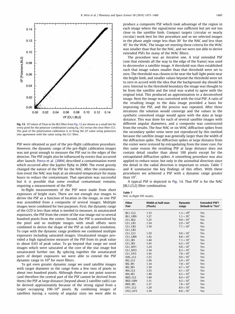
Fig. 13. I/F values of Titan in the BL2 filter from Fig. 12 are shown as a small dot for

every pixel for the polarizer combination (using Eq. (4)) versus the clear filter CL1.

The goal of the polarization calibration is to bring the I/F value using polarizers

into agreement with the value using the CL1 filter.

Table 7NAC in-flight PSF results.

FilterPair

Width at half-max(Pixels)

Dynamicrange

Extended PSF?Default is ‘‘Yes’’

BL1_CL2 1.33 1.3�108 Yes

BL1_GRN 1.27 1.1�107 Yes

CL1_BL2 1.25 9.0�107 Yes

CL1_CB1 1.34 2.9�103 No

CL1_CB2 1.39 7.7�107 Yes

CL1_CB3 Yes

CL1_CL2 1.29 9.0�107 Yes

CL1_GRN 1.42 8.8�107 Yes

CL1_IR1 1.44 7.1�107 Yes

CL1_IR3 1.45 6.2�107 Yes

CL1_MT1 1.24 9.8�107 Yes

CL1_MT2 1.34 8.3�107 Yes

CL1_UV3 1.45 7.8�107 Yes

HAL_CL2 1.25 9.0�107 Yes

IR2_CL2 1.56 5.9�107 Yes

IR2_IR1 1.34 7.8�107 Yes

IR2_IR3 1.39 6.7�107 Yes

IR4_CL2 1.53 6.1�107 Yes

IR4_IR3 1.40 6.5�107 Yes

RED_CL2 1.40 8.4�107 Yes

RED_GRN 1.31 9.2�107 Yes

RED_IR1 1.37 7.8�107 Yes

UV1_CL2 1.29 8.9�107 Yes

UV2_UV3 1.34 8.6�107 Yes

R. West et al. / Planetary and Space Science 58 (2010) 1475–1488 1485

PSF were obtained as part of the pre-flight calibration procedure.However, the dynamic range of the pre-flight calibration imageswas not great enough to measure the PSF out to the edges of thedetector. The PSF might also be influenced by events that occurredafter launch. Porco et al. (2004) described a contamination eventwhich occurred after the Jupiter flyby in 2000. The event grosslychanged the nature of the PSF for the NAC. After the contamina-tion event the NAC was kept at an elevated temperature for manyhours to reduce the contaminant. That operation was successfulbut it is possible that some residual contaminant remains,requiring a measurement of the PSF.

In-flight measurements of the PSF were made from shortexposures of bright stars. There are not enough star images toderive the PSF as a function of location in the image, so one PSFwas assembled from a composite of several images. Multipleimages were combined for two purposes. First, the dynamic rangeof the CCD is less than what is needed to measure, in unsaturatedexposures, the PSF from the center of the star image out to severalhundred pixels from the center. Second, the PSF is unresolved bythe pixel and so multiple images with small offsets werecombined to derive the shape of the PSF at sub-pixel resolution.To cope with the dynamic range problem we combined multipleexposures including saturated images. Unsaturated images pro-vided a high signal/noise measure of the PSF from its peak valueto about 0.03 of peak value. To go beyond that range we usedimages which were saturated at the core of the star image butunsaturated further out. By splicing together the unsaturatedparts of deeper exposures we were able to extend the PSFdynamic range to 104 for most filters.

To get even greater dynamic range we used satellite imageswith target diameter in the range from a few tens of pixels toabout two hundred pixels. Although these are not point sources(and therefore the central part of the PSF cannot be derived fromthem) the PSF at large distance (beyond about 2 satellite radii) canbe derived approximately because of the strong signal from atarget occupying 100–104 pixels. By combining images ofsatellites having a variety of angular sizes we were able to

produce a composite PSF which took advantage of the region ineach image where the signal/noise was sufficient but yet not tooclose to the satellite limb. Compact targets (circular or nearlycircular) work best for this procedure and so we selected imagesin the phase angle range less than 301 for the NAC and less than451 for the WAC. The image set meeting these criteria for the WACwas smaller than that for the NAC, and we were not able to deriveextended PSFs for many of the WAC filters.

The procedure was an iterative one. A trial extended PSF(one that extends all the way to the edge of the frame) was usedto deconvolve a satellite image. A threshold was then establishedsuch that image values smaller than that threshold were set tozero. The threshold was chosen to be near the half-light point nearthe bright limb, and smaller values beyond the threshold were setto zero in accord with the idea that the background sky should bezero. Internal to the threshold boundary the image was thought tobe from the satellite and the total was scaled to agree with theoriginal total. This produced an approximation to a deconvolvedimage. Next the image was convolved with the trial PSF. A ratio ofthe resulting image to the data image provided a basis forimproving the PSF, and the process was repeated. After threeiterations the solution would converge and the values in thesynthetic convolved image would agree with the data at largedistance. This was done for each of several satellite images withdifferent angular diameters, and a composite was constructedfrom the results. The four NAC or six WAC diffraction spikes fromthe secondary spider veins were not reproduced by this methodbecause the satellite image was generally larger than the width ofthe diffraction spike. The diffraction spikes at large distance fromthe center were restored by extrapolating from the inner core. Forthis same reason the resulting PSF at large distance does notcontain detail smaller than about 100 pixels except for theextrapolated diffraction spikes. A smoothing procedure was alsoapplied to reduce noise, but only in the azimuthal direction sincethe detail in the radial direction is important to retain. Table 7and 8 summarize the key findings of this effort. With theseprocedures we achieved a PSF with a dynamic range greaterthan 107.

A typical PSF is depicted in Fig. 14. That PSF is for the NAC[BL1,CL2] filter combination.

Fig. 15. An unusual PSF, for the NAC filter pair [BL1,GRN], which has a ghost

feature a few tens of pixels away from the main peak and with an amplitude

approximately 1% of the main peak. Such a feature is also seen in the [CL1,GRN]

filter pair but not in other filter .

Fig. 16. Diametric profile across the horizontal direction of the NAC PSF for the

narrow-band HAL-CL2 filter combination (dashed curve) and a theoretical PSF

based on a diffraction calculation at the same mean wavelength.

Table 8WAC in-flight PSF results.

Filterpair

Width at half-max(Pixels)

Dynamicrange

Extended PSF?Default is ‘‘Yes’’

CB2_CL2 1.38 3.6�107 No

CB3_CL2 1.77 2.1�107 No

CL1_BL1 1.46 2.2�107 Yes

CL1_CL2 1.72 1.8�107 Yes

CL1_GRN 1.19 4.9�107 Yes

CL1_HAL 1.08 1.4�108 No

CL1_IR1 1.57 4.3�107 Yes

CL1_RED 1.41 3.4�107 Yes

CL1_VIO 1.12 2.1�107 Yes

IR2_CL2 1.61 6.3�107 No

IR2_IR1 4.67 3.1�106 No

IR3_CL2 1.49 2.6�107 Yes

IR4_CL2 1.48 3.7�107 No

IR5_CL2 1.37 4.7�107 No

MT2_CL2 1.34 1.5�108 No

MT3_CL2 1.64 3.6�107 No

Fig. 14. A typical PSF for the NAC (rendered on a base-10 logarithmic scale), in this

case for filter pair [BL1,CL2]. The vertical axis is the base-10 logarithm of the PSF.

R. West et al. / Planetary and Space Science 58 (2010) 1475–14881486

Fig. 12. The images in the top half show the intensity of Titanat phase angle 1061. On the left is I/F from one NAC image(N1617163704) using the filter combination [CL1,BL2]. On theright is I/F derived from BL2 with three polarizers given by Eq. (4).In both cases the brightest pixels correspond to I/F¼0.14. Thebottom half of the image shows the degree of linear polarization(left side) and angle of polarization. The left image is scaled suchthat the brightest pixel corresponds to degree of polarization¼75%. The angle of polarization is close to 0 (electric vectorperpendicular to the sun direction) with maximum deviationabout 73.51 near the poles.

The NAC Green filter PSF exhibits a subsidiary peak (a ghostimage) as shown in Fig. 15.

The subsidiary peak is seen in combination with BL1 and alsowith the clear filter in the first filter wheel. It is probably due to aninternal reflection. We do not understand why this would be thecase only for the Green filter. More generally, internal reflectionsand stray light from the camera structure are probably respon-sible for the slow fall-off of the PSF at distances greater than a few

pixels. Figs. 16 and 17 show how the measured PSF at redwavelengths compares to a PSF computed from the diffractionpattern of an annulus whose outer diameter is the diameter of theprimary and whose inner diameter is that of the secondary mount(lamp holder in the case of the WAC). At large distance from thecenter the measured PSF is orders of magnitude larger than thediffraction-limited PSF. Heavily exposed images and images

Fig. 17. Diametric profile across the horizontal direction of the WAC PSF for the

CL1-RED filter combination (dashed curve) and a theoretical PSF based on a

diffraction calculation at the same mean wavelength.

Fig. 18. Example of diagonal streak from stray light in a NAC image

(N1472601232). This streak is produced by the satellite Tethys, which lies less

than 1/2 of a NAC FOV off of the upper left corner of this image.

R. West et al. / Planetary and Space Science 58 (2010) 1475–1488 1487

within 15–201 of the sun show stray light with complicatedpatterns. These patterns move and change depending on theapparent position of the light source. Our measured PSFs at largedistances are a smoothed average using several images.

There is one other filter combination that exhibits anomalousproperties. The WAC [IR2,IR1] combination has a PSF core that issignificantly wider than all other WAC filter combinations (widthat half maximum is almost five pixels). Because the WAC has arefractive objective it was not possible to bring all wavelengths toa common focus. The CL1 and CL2 filter thicknesses wereindividually optimized for best focus with the bandpass filtersin the opposite wheel. The [IR2,IR1] combination is unable to takeadvantage of that optimization.

Fig. 19. Example of the diffuse patterns observed at moderate phase in the WAC.

This image (W1486510390) shows the ansa of the E-ring at a vertically oriented

bright feature near the top of the frame. The horizontal bands and the diffuse

curving patterns extending over the image are attributed to stray light from the

bright rings and planet that lie off the top edge of this image.

10. Stray light

Stray light is present when light is scattered onto the detectorsby surfaces within or surrounding the cameras. Unlike theextended point spread function, the signal due to stray lightdepends not only on the pixel’s distance from the source but alsothe orientation of the entire camera relative to the source. Theseartifacts are therefore very difficult to model, and we have not yetbeen able to develop a generic procedure for identifying orremoving them. We will therefore simply review some propertiesof the stray light patterns we have identified in images takenduring the Cassini Mission.

Some of the most prominent stray-light artifacts occur whenrelatively bright, compact sources (like moons or nearly edge-onrings) lie just outside the camera’s field of view. These stray-lightartifacts can possess a great deal of fine-scale structure thatchanges as the off-image object moves relative to the field ofview. For the NAC, a bright object that lies just off the edge of theframe gives rise to bright streaks extending perpendicularly to therelevant edge, as well as more diffuse arc-like patterns

(c.f. Fig. 34A of Porco et al. 2004). Also, when a bright object islocated near to the corners of the NAC frame, a bright streak canbe seen to extend diagonally across the field of view (see Fig. 18).Similarly discrete features can be seen in some WAC images,along with more diffuse patterns that extend over the entire fieldof view (see Fig. 19). Some of the fine-scale structure in theseartifacts becomes washed out when the apparent size of theoff-axis sources is sufficiently large compared to the field of view,but there are also cases where stray light patterns persist in the

Fig. 20. The frame-average background sky brightness levels in the NAC and WAC

as a function of angular separation from the Sun. This plot was made using a

dedicated series of observations obtained on day 196 of 2002 and day 334 of 2003,

during Cassini’s cruise towards Saturn. The background sky brightness rises by

several orders of magnitude between 70 and 201, reaching an I/F level of nearly 0.1

in the WAC when the camera is pointed within 201 from the Sun (the WAC

saturated at 151 from the sun), and the NAC pointed to within 151 of the sun. The

sky brightness in the NAC is roughly three orders of magnitude lower than it is in

the WAC.

R. West et al. / Planetary and Space Science 58 (2010) 1475–14881488

images even when the source of the stray light is spatiallyextended. (For example, diagonal bands can be seen in close-upNAC images taken near the Saturn’s bright limb.) The techniquesrequired to remove these stray light patterns will thereforenecessarily be highly context-dependent, but in many casesappropriate spatial filtering techniques should allow faintsignals to be isolated from all but the worst of the artifacts.

In addition to the various structures visible within the images,stray light also contributes to the mean background signal in theimages. Fig. 20 shows the measured background sky brightness inthe cameras as a function of the cameras’ orientation relative to theSun, based on data from a specially designed imaging sequenceobtained while the spacecraft was cruising towards Saturn. Thesedata clearly show that the stray light levels in both camerasincrease as the camera points closer to the sun, and that the straylight levels in the WAC are roughly three orders of magnitudehigher than those of the NAC. In the WAC at least, the stray lightlevels seem to be somewhat higher in the infrared than the visible,which implies that the surfaces responsible for scattering thesunlight into the camera are more reflective at longer wavelengths.Other observations demonstrate that the brightness levels in bothcameras depend not only on the angle of the camera axis relative tothe sun, but also the azimuthal orientation of the camera (suchvariations are not apparent in Fig. 20 because these data come froma limited range of azimuthal angles).

We have not yet developed a complete model of the stray lightbrightness as a function of camera orientation and wavelength.However, as a practical matter the stray light levels in the NAC aresufficiently low that they do not seriously affect the ability of thecamera to image faint objects. By contrast, the high backgroundsobserved in the WAC (with background I/F values approaching 0.1 at201 from the Sun) render it almost unusable for faint targets likediffuse rings or auroras at phase angles greater than 1501 (unless thelight from the sun is blocked from the camera by the Saturn).

11. Future work

New calibration images will be taken to fill gaps in the currentcalibration files (such as missing distant PSFs for some filters in

Tables 7 and 8 and dust ring maps for the WAC). We plan toperiodically update the hot pixel maps and the dust ring maps,and to check for changes in the photometric performance andcharge transfer efficiency. Some of these, especially flat fieldimages for the WAC, will require images close to Titan where thecompetition for spacecraft resources is intense, and it is not clearif a sufficient number of calibration images will be obtained. Inaddition, we continue to seek answers to the puzzles emergingfrom this effort. We would like to be able to account for thelarger-than-expected variance of the stellar photometry. Wewould like to gain an understanding of what is responsible forthe ghost image with the GRN filter and why it is not seen in otherfilters.

Acknowledgements

We are grateful to a number of people who have contributed tothis work: Vance Haemmerle, Charles Avis, Philip Dumont, JeffCuzzi, S. Tom Elliott, Mike Evans, James Gerhard, Cynthia Kahn,Colin Mitchell, Keith Noll (who supplied the Enceladus spectrum),Kacie Shelton, and John Weiss. This research was carried out inpart at the Jet Propulsion Laboratory, California Institute ofTechnology, under a contract with the National Aeronautics andSpace Administration.

References

Alekseeva, G.A. Arkharov, A.A. Galkin, V.D. Hagen-Thorn, E.I., Nikanorova, I.N.,Novikov, V.V., Novopashenny, V.B., Pakhomov, V.P., Ruban, E.V., Shchegolev,D.E. 1997. Pulkovo Spectrophotometric Catalog. VizieR Catalog: III/201.

Bohlin, R.C., Gilliland, R.L., 2004. Hubble space telescope absolute spectro-photometry of Vega from the far-ultraviolet to the infrared. Astron. J. 127,3508–3515.

Burnashev, V.I. 1985. Catalogue of data on energy distribution in spectra of stars ina uniform spectrophotometric system, Abastumanskaya Astrofiz. Obs. Bull. 59,83-90. VizieR catalog III/126.

Glushneva, I.N., Doroshenko, V.T., Fetisova, T.S., Khruzina, T.S., Kolotilov, E.A.,Mossakovskaya, L.V., Shenavrin, V.I., Voloshina, I.B., Biryukov, V.V., Shenavrina,L.S. 1998a. Moscow Spectrophotometric Catalog of Stars. VizieR Catalog III/207.

Glushneva, I.N., Doroshenko, V.T., Fetisova, T.S., Khruzina, T.S., Kolotilov, E.A.,Mossakovskaya, L.V., Ovchinnikov, S.L., Voloshina, I.B. 1998b. SternbergSpectrophotometric Catalog. VizieR Catalog: III/208.

Gunn, J.E., Stryker, L.L., 1983. Stellar spectrophotometric atlas, wavelengths from3130 to 10800 A. Astrophys. J. Suppl. Ser. 52, 121–153.

Hamuy, M., Walker, A.R., Suntzeff, N.B., Gigoux, P., Heathcote, S.R., Phillips, M.M.,1992. Southern spectrophotometric standards. Astron. Soc. Pacific 104,533–552.

Hamuy, M., Suntzeff, N.B., Heathcote, S.R., Walker, A.R., Gigoux, P., Phillips, M.M., 1994.Southern spectrophotometric standards. 2. Astron. Soc. Pacific 106, 566–589.

Hansen, J.E., Travis, L.D., 1974. Light-scattering in planetary atmospheres. SpaceSci. Rev. 16, 527–610.

Heck, A., Egret, D., Jaschek, C., Battrick, B. 1984. IUE low dispersion spectrareference atlas. Part 1: normal stars. IUE low dispersion spectra referenceatlas. Part 1: normal stars. ESA Special Publication: ESA SP-1052, ISSN0379-6566.

Jamar, C., Macau-Hercot, D., Monfils, A., Thompson, G.I., Houziaux, L., Wilson, R.1976. UV Bright Star Spectrophotometric Catalog. VizieR On-line Data Catalog:III/39A.

Kharitonov, A.V., Tereshchenko, V.M., Knyazeva, L.N., 1988. SpectrophotometricCatalogue of Stars. VizieR Catalog III/202. Alma-Ata, Nauka, p. 484.

Kurucz, R.L. 1993. Model Atmospheres. VizieR On-line Data Catalog: VI/39.Originally published in: 1979 Ap. J. Supp.

Ochsenbein, F., Bauer, P., Marcout, J., 2000. The VizieR database of astronomicalcatalogues. Astron. Astrophys. Suppl. 143, 23–32.

Porco, C.C., West, R.A., Squyres, S., McEwen, A., Thomas, P., Murray, C.D., DelGenio,A., Ingersoll, A.P., Johnson, T.V., Neukum, G., Veverka, J., Dones, L., Brahic, A.,Burns, J.A., Haemmerle, V., Knowles, B., Dawson, D., Roatsch, T., Beurle, K.,Owen, W., 2004. Cassini imaging science: instrument characteristicsand anticipated scientific investigations at Saturn. Space Sci. Rev. 115,363–497.

Santos, J.F.C., Jr., Alloin, D., Bica, E., Bonatto, C. 2001. Spectral Library of Galaxies,Clusters and Stars. VizieR On-line Data Catalog: III/219.

Stokes, G.G., 1860. On the intensity of the light reflected from or transmittedthrough a pile of plates. Proc. Roy. Soc. London 11, 545–557.