General rights Copyright and moral rights for the publications made accessible in the public portal are retained by the authors and/or other copyright owners and it is a condition of accessing publications that users recognise and abide by the legal requirements associated with these rights.

• Users may download and print one copy of any publication from the public portal for the purpose of private study or research. • You may not further distribute the material or use it for any profit-making activity or commercial gain • You may freely distribute the URL identifying the publication in the public portal

If you believe that this document breaches copyright please contact us providing details, and we will remove access to the work immediately and investigate your claim.

Downloaded from orbit.dtu.dk on: Sep 22, 2018

HFI energetic particle effects: characterization, removal, and simulation

Ade, P. A. R.; Aghanim, N.; Armitage-Caplan, C.; Arnaud, M.; Ashdown, M.; Atrio-Barandela, F.; Aumont,J.; Baccigalupi, C.; Banday, A. J.; Barreiro, R. B.; Battaner, E.; Benabed, K.; Benoit, A.; Benoit-Levy, A.;Bernard, J. -P.; Bersanelli, M.; Bielewicz, P.; Bobin, J.; Bock, J. J.; Bond, J. R.; Borrill, J.; Bouchet, F. R.;Bridges, M.; Bucher, M.; Burigana, C.; Cardoso, J. F.; Catalano, A.; Challinor, A.; Chamballu, A.; Chiang,H. C.; Chiang, L. -Y.; Christensen, P. R.; Church, S.; Clements, D. L.; Colombi, S.; Colombo, L. P. L.;Couchot, F.; Coulais, A.; Crill, P.; Curto, A.; Cuttaia, F.; Danese, L.; Davies, R. D.; de Bernardis, P.; deRosa, A.; de Zotti, G.; Delabrouille, J.; Delouis, J. -M.; Desert, F. -X.; Diego, J. M.; Dole, H.; Donzelli, S.;Dore, O.; Douspis, M.; Dupac, X.; Efstathiou, G.; Ensslin, T. A.; Appelby Hansen, Heidi; Finelli, F.; Forni,O.; Frailis, M.; Franceschi, E.; Galeotta, S.; Gana, K.; Giard, M.; Girard, D.; Giraud-Heraud, Y.; Gonzalez-Nuevo, J.; Gorski, K. M.; Gratton, S.; Gregorio, A.; Gruppuso, A.; Hansen, F. K.; Hanson, D.; Harrison, D.;Henrot-Versille, S.; Hernandez-Monteagudo, C.; Herranz, D.; Hildebrandt, S. R.; Hivon, E.; Hobson, M.;Holmes, W. A.; Hornstrup, Allan; Hovest, W.; Huffenberger, K. M.; Jaffe, A. H.; Jaffe, T. R.; Jones, W. C.;Juvela, M.; Keihanen, E.; Keskitalo, R.; Kisner, T. S.; Kneissl, R.; Knoche, J.; Knox, L.; Kunz, M.; Kurki-Suonio, H.; Lagache, G.; Lamarre, J. -M.; Lasenby, A.; Laureijs, R. J.; Lawrence, C. R.; Leonardi, R.;Leroy, C.; Lesgourgues, J.; Liguori, M.; Lilje, P. B.; Linden-Vørnle, Michael; Lopez-Caniego, M.; Lubin, P.M.; Macias-Perez, J. F.; Mandolesi, N.; Maris, M.; Marshall, D. J.; Martin, P. G.; Martinez-Gonzalez, E.;Masi, S.; Massardi, M.; Matarrese, S.; Matthai, F.; Mazzotta, P.; McGehee, P.; Melchiorri, A.; Mendes, L.;Mennella, A.; Migliaccio, M.; Miniussi, A.; Mitra, A.; Miville-Deschenes, M. A.; Moneti, A.; Montier, L.;Morgante, G.; Mortlock, D.; Mottet, S.; Munshi, D.; Murphy, J. A.; Naselsky, P.; Nati, F.; Natoli, P.;Netterfield, C. B.; Nørgaard-Nielsen, Hans Ulrik; Noviello, F.; Novikov, D.; Novikov, I.; Osborne, S.;Oxborrow, Carol Anne; Paci, F.; Pagano, L.; Pajot, Fernand; Paoletti, D.; Patanchon, G.; Perdereau, O.;Perotto, L.; Perrotta, F.; Piacentini, F.; Piat, M.; Pierpaoli, E.; Pietrobon, D.; Plaszczynski, S.;Pointecouteau, E.; Polenta, G.; Ponthieu, N.; Popa, L.; Poutanen, T.; Pratt, G. W.; Prezeau, G.; Prunet, S.;Puget, J. -L.; Rachen, J. P.; Racine, B.; Reinecke, M.; Remazeilles, M.; Renault, C.; Ricciardi, S.; Riller, T.;Ristorcelli, I.; Rocha, G.; Rosset, C.; Roudier, G.; Rusholme, B.; Sanselme, L.; Santos, D.; Sauve, A.;Savini, G.; Scott, D.; Shellard, E. P. S.; Spencer, L. D.; Starck, J. -L.; Stolyarov, V.; Stompor, R.; Sudiwala,R.; Sureau, F.; Sutton, D.; Suur-Uski, A. S.; Sygnet, J. -F.; Tauber, J. A.; Tavagnacco, D.; Terenzi, L.;Toffolatti, L.; Tomasi, M.; Tristram, M.; Tucci, M.; Umana, G.; Valenziano, L.; Valiviita, J.; Van Tent, B.;Vielva, P.; Villa, F.; Vittorio, N.; Wade, L. A.; Wandelt, B. D.; Yvon, D.; Zacchei, A.; Zonca, A.Published in:Astronomy & Astrophysics

Link to article, DOI:10.1051/0004-6361/201321577

Publication date:2014

Document VersionPublisher's PDF, also known as Version of record

Link back to DTU Orbit

A&A 571, A10 (2014)DOI: 10.1051/0004-6361/201321577c© ESO 2014

Astronomy&

AstrophysicsPlanck 2013 results Special feature

Planck 2013 results. X. HFI energetic particle effects:characterization, removal, and simulation

Planck Collaboration: P. A. R. Ade83, N. Aghanim58, C. Armitage-Caplan87, M. Arnaud70, M. Ashdown67,6, F. Atrio-Barandela18, J. Aumont58,C. Baccigalupi82, A. J. Banday90,10, R. B. Barreiro64, E. Battaner91, K. Benabed59,89, A. Benoît56, A. Benoit-Lévy25,59,89, J.-P. Bernard90,10,

M. Bersanelli35,49, P. Bielewicz90,10,82, J. Bobin70, J. J. Bock65,11, J. R. Bond9, J. Borrill14,84, F. R. Bouchet59,89, M. Bridges67,6,62, M. Bucher1,C. Burigana48,33, J.-F. Cardoso71,1,59, A. Catalano72,69, A. Challinor62,67,12, A. Chamballu70,15,58, H. C. Chiang28,7, L.-Y Chiang61,

P. R. Christensen78,38, S. Church86, D. L. Clements54, S. Colombi59,89, L. P. L. Colombo24,65, F. Couchot68, A. Coulais69, B. P. Crill65,79,A. Curto6,64, F. Cuttaia48, L. Danese82, R. D. Davies66, P. de Bernardis34, A. de Rosa48, G. de Zotti44,82, J. Delabrouille1, J.-M. Delouis59,89,

F.-X. Désert52, J. M. Diego64, H. Dole58,57, S. Donzelli49, O. Doré65,11, M. Douspis58, X. Dupac40, G. Efstathiou62, T. A. Enßlin75, H. K. Eriksen63,F. Finelli48,50, O. Forni90,10, M. Frailis46, E. Franceschi48, S. Galeotta46, K. Ganga1, M. Giard90,10, D. Girard72, Y. Giraud-Héraud1,

J. González-Nuevo64,82, K. M. Górski65,92, S. Gratton67,62, A. Gregorio36,46, A. Gruppuso48, F. K. Hansen63, D. Hanson76,65,9, D. Harrison62,67,S. Henrot-Versillé68, C. Hernández-Monteagudo13,75, D. Herranz64, S. R. Hildebrandt11, E. Hivon59,89, M. Hobson6, W. A. Holmes65,

A. Hornstrup16, W. Hovest75, K. M. Huffenberger26, A. H. Jaffe54, T. R. Jaffe90,10, W. C. Jones28, M. Juvela27, E. Keihänen27, R. Keskitalo22,14,T. S. Kisner74, R. Kneissl39,8, J. Knoche75, L. Knox29, M. Kunz17,58,3, H. Kurki-Suonio27,42, G. Lagache58, J.-M. Lamarre69, A. Lasenby6,67,

R. J. Laureijs41, C. R. Lawrence65, R. Leonardi40, C. Leroy58,90,10, J. Lesgourgues88,81, M. Liguori32, P. B. Lilje63, M. Linden-Vørnle16,M. López-Caniego64, P. M. Lubin30, J. F. Macías-Pérez72, N. Mandolesi48,5,33, M. Maris46, D. J. Marshall70, P. G. Martin9,

E. Martínez-González64, S. Masi34, M. Massardi47, S. Matarrese32, F. Matthai75, P. Mazzotta37, P. McGehee55, A. Melchiorri34,51, L. Mendes40,A. Mennella35,49, M. Migliaccio62,67, A. Miniussi58, S. Mitra53,65, M.-A. Miville-Deschênes58,9, A. Moneti59, L. Montier90,10, G. Morgante48,

D. Mortlock54, S. Mottet59, D. Munshi83, J. A. Murphy77, P. Naselsky78,38, F. Nati34, P. Natoli33,4,48, C. B. Netterfield20, H. U. Nørgaard-Nielsen16,F. Noviello66, D. Novikov54, I. Novikov78, S. Osborne86, C. A. Oxborrow16, F. Paci82, L. Pagano34,51, F. Pajot58, D. Paoletti48,50, F. Pasian46,

G. Patanchon1,?, O. Perdereau68, L. Perotto72, F. Perrotta82, F. Piacentini34, M. Piat1, E. Pierpaoli24, D. Pietrobon65, S. Plaszczynski68,E. Pointecouteau90,10, G. Polenta4,45, N. Ponthieu58,52, L. Popa60, T. Poutanen42,27,2, G. W. Pratt70, G. Prézeau11,65, S. Prunet59,89, J.-L. Puget58,J. P. Rachen21,75, B. Racine1, M. Reinecke75, M. Remazeilles66,58,1, C. Renault72, S. Ricciardi48, T. Riller75, I. Ristorcelli90,10, G. Rocha65,11,

C. Rosset1, G. Roudier1,69,65, B. Rusholme55, L. Sanselme72, D. Santos72, A. Sauvé90,10, G. Savini80, D. Scott23, E. P. S. Shellard12,L. D. Spencer83, J.-L. Starck70, V. Stolyarov6,67,85, R. Stompor1, R. Sudiwala83, F. Sureau70, D. Sutton62,67, A.-S. Suur-Uski27,42, J.-F. Sygnet59,

J. A. Tauber41, D. Tavagnacco46,36, L. Terenzi48, L. Toffolatti19,64, M. Tomasi49, M. Tristram68, M. Tucci17,68, G. Umana43, L. Valenziano48,J. Valiviita42,27,63, B. Van Tent73, P. Vielva64, F. Villa48, N. Vittorio37, L. A. Wade65, B. D. Wandelt59,89,31, D. Yvon15, A. Zacchei46, and A. Zonca30

(Affiliations can be found after the references)

Received 26 March 2013 / Accepted 1 July 2014

ABSTRACT

We describe the detection, interpretation, and removal of the signal resulting from interactions of high energy particles with the Planck HighFrequency Instrument (HFI). There are two types of interactions: heating of the 0.1 K bolometer plate; and glitches in each detector time stream.The transient responses to detector glitch shapes are not simple single-pole exponential decays and fall into three families. The glitch shape foreach family has been characterized empirically in flight data and these shapes have been used to remove glitches from the detector time streams.The spectrum of the count rate per unit energy is computed for each family and a correspondence is made to the location on the detector of theparticle hit. Most of the detected glitches are from Galactic protons incident on the die frame supporting the micro-machined bolometric detectors.In the Planck orbit at L2, the particle flux is around 5 cm−2 s−1 and is dominated by protons incident on the spacecraft with energy >39 MeV,at a rate of typically one event per second per detector. Different categories of glitches have different signatures in the time stream. Two of theglitch types have a low amplitude component that decays over nearly 1 s. This component produces excess noise if not properly removed fromthe time-ordered data. We have used a glitch detection and subtraction method based on the joint fit of population templates. The application ofthis novel glitch subtraction method removes excess noise from the time streams. Using realistic simulations, we find that this method does notintroduce signal bias into the Planck data.

Key words. cosmic background radiation – cosmology: observations – instrumentation: detectors – space vehicles: instruments –methods: data analysis

? Corresponding author: G. Patanchon, e-mail: patanchon@apc.univ-paris-Diderot.fr

Article published by EDP Sciences A10, page 1 of 23

A&A 571, A10 (2014)

1. Introduction

This paper, one of a set associated with the 2013 release of datafrom the Planck1 mission (Planck Collaboration I 2014), de-scribes the detection of high energy particle impacts on the 0.1 Kstage and bolometric detectors in the Planck High FrequencyInstrument (HFI, Lamarre et al. 2010) and removal of these sys-tematic effects from the millimetre and submillimetre signals.A full description of the HFI can be found elsewhere (PlanckHFI Core Team 2011a,b; Planck Collaboration VI 2014;Planck Collaboration VII 2014; Planck Collaboration VIII 2014;Planck Collaboration IX 2014).

Bolometers (Holmes et al. 2008), such as those used in HFIon Planck, are phonon-mediated thermal detectors with finiteresponse time to changes in the absorbed optical power. Thebolometer consists of a micro-machined silicon nitride (Si-N)mesh absorber with a germanium (Ge) thermistor suspendedfrom the Si die frame. Each bolometer is mounted on a metalhousing, and these are assembled into two types of bolometermodules, as shown in Fig. 1: a spider web bolometer (SWB,Bock et al. 1995) which detects total power; and a polarizationsensitive bolometer (PSB, Jones et al. 2007). In the PSB mod-ule there are two bolometers to independently measure power ineach of the two linear polarizations. The bolometers are mountedon a copper-plated stainless steel plate cooled to 0.1 K and stabi-lized within a few microkelvin of the temperature set point. Two“dark” bolometer modules are blanked off at the 0.1 K plate andare used to monitor systematic effects. The 0.1 K bolometer plateis surrounded by a roughly 1.5 mm thick aluminium box cooledto 4.5 K. Light is coupled into each bolometer module using afeedhorn at 4.5 K and a filter stack at 1.5 K (Lamarre et al. 2010).

At the Earth-Sun Lagrange point L2, high energy particlesfrom the Sun and Galactic sources – primarily protons, electronsand helium nuclei – are incident on the spacecraft. This particleflux causes two main effects in HFI that have been reported pre-viously. There is a time-variable thermal load on the 0.1 K plate(Planck Collaboration II 2011) and a significant rate of glitchesin the bolometric signal (Planck HFI Core Team 2011b). In thispaper, we report on the evolution of these effects over the en-tire period of HFI operations, from 3 July 2009 to 14 January2012, and describe the analysis technique used to remove the ef-fect of glitches from the data. Three families of glitches, “long”,“short”, and “slow” (or “longer” as named in Planck HFI CoreTeam 2011b), were found by comparing and stacking manyevents. Their characteristics are detailed in Sect. 2. Long glitchesdominate the overall counts and exhibit an additional slow decaywith a time constant of the order of 2 s, requiring template sub-traction from the data. The new analysis, presented in Sect. 3.1,employs a joint fitting of the three glitch family templates andremoval of the slow tails. In Sects. 3.2 and 4 we show that ouradopted technique improves the noise performance of HFI. Wehave simulated the effect of the glitches on the data quality andfind that systematic biases are small, contributing <10−4 to thecosmological power spectrum.

We also present the coincident counts, energy distribution,total counts, and variations of glitch shapes within each fam-ily. These data, taken together with the beam-line and laboratory

1 Planck (http://www.esa.int/Planck) is a project of theEuropean Space Agency (ESA) with instruments provided by two sci-entific consortia funded by ESA member states (in particular the leadcountries France and Italy), with contributions from NASA (USA) andtelescope reflectors provided by a collaboration between ESA and ascientific consortium led and funded by Denmark.

Backshort / Aft / b

Housing / Fore / a

Printed Wiring Board (PWB)

Cover

Fig. 1. Top left and right: completed multimode (see Maffei et al. 2010)545 GHz and single-mode 143 GHz SWB bolometer modules. Middle:an exploded view of the assembly of a PSB (showing the definition ofthe “a” and “b” detectors of the pair). Alignment pins, shown in solidblack, fix the aft and fore bolometer assemblies to an angular preci-sion of <0.1◦. The SWB assembly is similar to the PSB aft bolometerassembly and does not include a feedhorn aperture integrated with themodule package. Bottom: PSB pair epoxied in the module parts prior tomating. To the right, the feedhorn aperture can be seen through the forebolometer in the housing. To the left, the quarter-wave backshort can beseen through the aft bolometer absorber mesh.

tests using spare HFI bolometers (Catalano et al. 2014; PlanckCollaboration II 2011), allow identification of the physical causeof the glitch events for two of the types (Sect. 5). Long glitchesare due to energy absorption events in the Si die and shortglitches are due to events in the optical absorbing grid or Ge ther-mistor. The cause of the slow glitches, however, has not beenidentified. We also describe some rare effects not previously re-ported, including the response of the instrument to solar flares,secondary showers, and large high-energy events.

2. Glitch families

For instruments with bolometric detectors fielded on balloons(Crill et al. 2003; Masi et al. 2006; Benoît et al. 2003; Patanchonet al. 2008) and space missions (see Griffin et al. 2010, forHerschel-SPIRE), the glitches are flagged in the data time streamand then the flagged data are omitted. For most of these instru-ments, the transfer function is deconvolved from the time streamprior to flagging glitches. This has the benefit of increasing

A10, page 2 of 23

Planck Collaboration: Planck 2013 results. X.

10

-310

-210

-110

0

0.0 0.2 0.4 0.6 0.8 Time [s]

Glit

ch s

igna

ls /

max

[AD

U]

Fig. 2. Examples of three distinct families of glitch transfer functionsfor a typical PSB-a bolometer. Events like the blue curves are called“short” events, those like the black curves are called “long”, and thoselike the red curves are called “slow”. Typical variation of the shapewithin each family is shown for short and long glitches. The differencesbetween long glitch shapes are modelled by a single nonlinearity pa-rameter relating the amplitude of the slow tail of events with their peakamplitude. There is no apparent glitch tail associated with short events.

the signal-to-noise ratio on each glitch, which minimizes thefraction of falsely flagged data.

The population of glitches in Planck HFI is unusual. Theglitch rate of ∼1 s−1 per detector is significantly higher thanin the other instruments. Also, three distinct families of glitchtransfer functions, shown in Fig. 2, are present in the data. Thetransfer function of each glitch family is described by a sum ofthree or four decaying exponential terms. For a given bolome-ter, the families, called short, long, and slow, are differentiatedby the relative amplitudes of each term. Only the short glitcheshave a transfer function matching the instrument transfer func-tion. The long glitches dominate the total rate and have a signifi-cant amplitude above the noise level, with a time constant >1 s asillustrated in Fig. 2. Deconvolving the instrument transfer func-tion prior to glitch flagging did not improve glitch detection, andthe large amplitude at times >1 s, which is the typical time be-tween glitches, means there is glitch pile up. The high rate oflong glitches leads to considerable confusion of glitch signals,as can be seen in Fig. 3, and makes it difficult to clean glitchesin Planck-HFI data.

Omitting flagged data would lead to omission of >90% ofthe data, so we have developed a strategy to fit and to removeprecise templates of long glitches from the time-ordered data.We take advantage of the excellent pointing accuracy (PlanckCollaboration I 2011) and redundancy of the scan strategy, andhave adopted a method that iterates between estimates of thesignal from the sky and signal from the glitches (Planck HFICore Team 2011b). A key to the effectiveness of this method,presented in Sect. 3.1, is a comprehensive understanding of thethree families of glitches and a determination of the stability ofthese families over the course of the mission. In this section, wedescribe the features of the different glitch families that are rel-evant for their removal. Identification and classification of theglitches has been done using previous versions of the method,as introduced in Planck Collaboration VII (2014). This was aniterative process, since accurate glitch property determination isnecessary to “tune” the method for effective detection and clean-ing, and an efficient method is necessary to separate glitchesinto families and derive properties. Templates of each of the

-4

00

040

080

0

0 2 4 6 8 10Time [s]

Dat

a [A

DU

]

Fig. 3. Black: segment of raw data for one detector at 143 GHz be-fore any deglitching; an estimate of the sky signal has been subtracted.Red: a time stream reconstructed from the estimated templates of longglitches with the method presented in Sect. 3.1. We have chosen a regionin the vicinity of a large event. Data that are flagged for the analysis areindicated by the lines at the bottom of the figure. Notice the high levelof confusion between long glitch signals.

three glitch families are obtained from stacking many normal-ized glitches, and the general features are derived from fittingthe normalized decay profile with a sum of exponentials. Themethodology is detailed in Sect. 3.1.4.

2.1. Short glitches

The highest-amplitude events are the short glitches. The shortglitch time response, or template, is shown in Fig. 4. Short eventshave a rise time much shorter than the sampling period of 5 ms,followed by a fast decay. These rapid variations can cause oscil-lations in the electronics, and the response amplitude depends onthe precise moment of the glitch within the sampling period. Sothroughout the paper, the amplitude of the glitch is defined as thepeak value of the sampled data. The shortest exponential decaycomponent has a time constant similar to the fast part of the op-tical transfer function; three additional terms (corresponding tothe tail) have very low amplitudes (<10−2 of the peak), and timeconstants of typically 40 ms, 400 ms, and 2 s. The 2 s decayingsignal has an amplitude about 5 × 10−5 of the peak and was de-tected only after stacking short glitches measured over the entiremission. The transfer function of short glitches nearly matchesthe instrument optical transfer function.

The time constants and amplitudes derived by fitting threeexponentials to short glitch measurements are given in Fig. 5for all the bolometers. The fit has been performed after stackingevents with amplitudes between 1200 and 2400 times the noise(around 2 keV of deposited energy), which corresponds to en-ergies of the transition between the two subcategories of shortevents. The 2 s time constant is not included in the template fit.We have verified that, given the counts of short glitches, andassuming a random distribution of glitches, the 2 s tails pro-duce a signal that is three orders of magnitude lower than thewhite noise, and so can be neglected in the data processing. Weobserve some scatter of the values across bolometers, althoughthis may reflect the degeneracies in the fit of the different timeconstants and amplitudes rather than variations of the templateshape between bolometers. A careful study of the degeneracies

A10, page 3 of 23

A&A 571, A10 (2014)

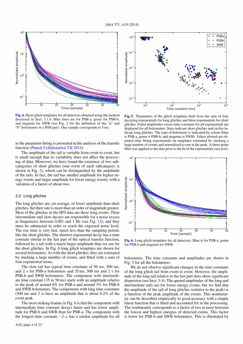
Fig. 4. Short glitch templates for all detectors obtained using the methoddiscussed in Sect. 3.1.4. Blue lines are for PSB-a, green for PSB-b,and magenta for SWB (see Fig. 2 for the definition of the “a” and“b” bolometers in a PSB pair). One sample corresponds to 5 ms.

in the parameter fitting is presented in the analysis of the transferfunction (Planck Collaboration VII 2014).

The amplitude of the tail is variable from event to event, butis small enough that its variability does not affect the process-ing of data. Moreover, we have found the existence of two sub-categories of short glitches (one event of each subcategory isshown in Fig. 2), which can be distinguished by the amplitudeof the tails. In fact, the tail has smaller amplitude for higher en-ergy events and larger amplitude for lower energy events, with avariation of a factor of about two.

2.2. Long glitches

The long glitches are, on average, of lower amplitude than shortglitches, but their rate is more than an order of magnitude greater.Most of the glitches in the HFI data are these long events. Theirintermediate and slow decays are responsible for a noise excessat frequencies between 0.001 and 1 Hz (see Fig. 12), and theymust be subtracted in order to reach the expected noise level.The rise time is very fast, much less than the sampling period,like the short glitches. The shortest exponential decay has a timeconstant similar to the fast part of the optical transfer function,followed by a tail with a much larger amplitude than we see forthe short glitches. In Fig. 6 long glitch templates are shown forseveral bolometers. As with the short glitches, they are estimatedby stacking a large number of events, and fitted with a sum offour exponential terms.

The slow tail has typical time constants of 50 ms, 500 ms,and 2 s for PSB-a bolometers and 35 ms, 500 ms and 2 s forPSB-b and SWB bolometers. The component with intermedi-ate time constant (35 to 50 ms) starts with an amplitude relativeto the peak of around 6% for PSB-a and around 3% for PSB-band SWB bolometers. The components with long time constants(500 ms and 2 s) have an amplitude that is about 0.2% of theevent peak.

The most striking feature in Fig. 6 is that the component withintermediate time constant decays faster and has lower ampli-tude for PSB-b and SWB than for PSB-a. The component withthe longest time constant, ∼2 s, has a similar amplitude for all

Fig. 5. Parameters of the glitch templates built from the sum of fourdecaying exponentials for long glitches and three exponentials for shortglitches. Fitted amplitudes versus time constants for all exponentials aredisplayed for all bolometers. Stars indicate short glitches and circles in-dicate long glitches. The type of bolometer is indicated by colour (blueis PSB-a, green is PSB-b, and magenta is SWB). Values plotted are ob-tained after fitting exponentials on templates estimated by stacking alarge number of events and normalized to one at the peak. A three-pointfilter was applied to the data prior to the fit of the exponentials (see text).

Fig. 6. Long glitch templates for all detectors. Blue is for PSB-a, greenfor PSB-b and magenta for SWB.

bolometers. The time constants and amplitudes are shown inFig. 5 for all the bolometers.

We do not observe significant changes in the time constantsof the long glitch tail from event to event. However, the ampli-tude of the long tail relative to the fast part does show significantdispersion (see Sect. 5.4). The quoted amplitudes of the long andintermediate tails are for lower energy events, but we find thatthe amplitude of the tail of long glitches (relative to the peak) isa function of the peak amplitude of the events. This nonlinear-ity can be described empirically to good accuracy with a simplelinear function that is fitted and accounted for in the processing.The nonlinearity corresponds to a factor of two at most betweenthe lowest and highest energies of detected events. This factoris lower for PSB-b and SWB bolometers. This is illustrated by

A10, page 4 of 23

Planck Collaboration: Planck 2013 results. X.

10

-310

-210

-110

0

0.0 0.5 1.0 1.5 Time [s]

Res

cale

d gl

itch

sign

al

Fig. 7. Comparison of a long glitch (black) and a slow glitch (dot-dashed blue). For this plot, the two high energy events were rescaledto match after 200 ms. The difference is shown in blue.

Fig. 2, which shows two typical long events at different ampli-tudes, both normalized to the peak. The difference in amplitudeof the slow tail is clearly visible.

Finally, in a small proportion of events the ratio of amplitudeof the fast part to that of the slow part is different from the major-ity of long glitches. In particular, slightly less than 10% of eventshave a smaller amplitude tail than long glitches and about 0.5%have a higher tail (not including slow glitches). Those events donot fit into any of the categories of glitches, but their slow decay-ing tails, after ≈20 ms from the peak amplitude, are similar to thelong glitches. Because of this, they are implicitly accounted forin the glitch removal procedure.

2.3. Slow glitches

Slow glitches are detected only for PSB-a. They have a rise timecomparable to the optical time constant, i.e., much slower thanthe two other glitch families. The tail of a slow glitch is similarto that of a long glitch. Figure 7 shows a comparison of a highamplitude long glitch event with a slow glitch. The intermediatetime constant of long glitches, which is of the order of 50 msfor PSB-a, is slightly (but significantly) larger for slow glitches,and this time constant is the fastest for those events, as can beseen in Fig. 7. The two tails are proportional to good accuracyfrom about 200 ms after the peak amplitude. Even with thesedifferences, the long glitch template for a given bolometer is agood proxy for the slow glitches in the same bolometer.

2.4. Population counts

Figure 8 shows the distribution dN/dE of the three populations ofglitches for one detector as a function of the amplitude of eventsin signal-to-noise ratio units. The type of each event is deter-mined by the method of Sect. 3.1. We can see that long glitchevents are dominant at lower amplitudes, while short eventsdominate at higher amplitudes. The separation between shortand long events is not efficient below about 20σ (i.e., 20 timesthe rms noise), because the tails of long glitches, used to dis-tinguish between the two types of events, are barely detectable.Nevertheless, we will see later that long glitches are dominant atlower amplitudes, as can be guessed by extrapolating the counts.Long glitches are dominant in the overall counts. The distri-bution of long glitches is well fitted by a steep power law of

10-6

10-4

10-2

100

102

104

101 102 103 104

Amplitude (signal to noise)

Num

ber

of e

vent

s / n

oise

rm

s/ h

our

TotalLongShortSlow

Fig. 8. Distributions, dN/dE, of the three families of glitches with re-spect to the peak amplitude, in signal-to-noise ratio units, for three dif-ferent bolometers: 143-1a; 143-2a; and 217-1. The blue line is for theshort glitch population, black is for long, red is for slow, and green is fortotal. We have chosen bolometers with very different behaviour: 143-1ahas one of the lowest glitch rates while 143-2a and 217-1 have highglitch rates. The faint-end break of the glitch counts is visible for 217-1,a bolometer that has no slow glitches (see Sect. 2.3). Power laws areshown for comparison as dashed lines. Indices and amplitudes of powerlaws are chosen to match the distribution of bolometer 143-2a. Indicesare −2.4 for long and slow glitches, and −1.7 for short glitches. The ver-tical dashed line indicates the detection threshold. There is no attempthere to separate the long and short glitch populations below 20 timesthe rms noise. The slow glitch spectrum is shown down to 5 times therms.

index −2.4 between typical amplitudes of 20 and 1000 timesthe rms noise (with some variations among bolometers), andshows breaks at both the bright and faint ends. The faint-endbreak is close to the glitch detection threshold, which is fixedat 3.2σ, and is detected very significantly (as we will discuss inSect. 5.4). The submillimetre channels (545 and 857 GHz) aremore sensitive to long glitches. For those detectors, we observea peak in the differential counts at energies close to the detectionthreshold. We will see in Sect. 5.4 that very few events are ex-pected below the detection threshold. We observe a large scatterfrom bolometer to bolometer in the amplitude scaling of the longglitch distribution, but the overall shape is preserved.

The distribution of short glitches has a bump at amplitudesaround 3000σ for all bolometers from 100 to 353 GHz. There isa clear break at very high amplitudes, which is mostly due to thenonlinearity of the detectors at those amplitudes and to the sat-uration of the analogue-to-digital convertor (ADC, see PlanckCollaboration VI 2014, for a discussion of the effect on the data).The bump in the distribution is not apparent in the submillimetredetectors, but this is due to the nonlinearity smearing it out. Foramplitudes below about 1000σ, the distribution of short glitchesis well represented by a power law with a typical index of −1.7.Short events with an energy corresponding to the bump appear tohave shorter timescales than events corresponding to the powerlaw.

The shapes of the distributions of slow and long glitches arevery similar. We see in Fig. 8 that long glitches are more nu-merous than slow glitches, but the distributions shown are nor-malized to the peaks of events. After rescaling on the amplitudeof the slow tails, which are similar for the two populations, theslow glitch distributions end up much closer to the long glitch

A10, page 5 of 23

A&A 571, A10 (2014)

Fig. 9. Glitch rates for each bolometer. Points represent the mean valuesduring each 6 month survey.

distributions. The slow glitches are then contributing very sig-nificantly to the noise power excess.

The glitch rates per bolometer are given in Fig. 9 for eachsix-month survey. Numbers are derived by integrating differen-tial counts down to the detection threshold. Long glitches dom-inate the counts. Variations across bolometers are mainly ex-plained by the differences in the sensitivity to long glitches.In particular, channels with lower rates also have more eventsbelow the detection threshold. As described in Holmes et al.(2008), bolometers in PSBs were selected from die on the samewafer. Also, attempts were made to select die from neighbor-ing locations on that same wafer. In 14 of 16 PSBs, the PSB-aand -b are from the same wafer. Due to limited yield, for 2 ofthe 100 GHz PSBs, 100-2 and 100-4, PSB-a and PSB-b arefrom different wafers. Nevertheless, as shown in Fig. 9 there isno significant difference between the bolometers in these twoPSBs compared to difference in bolometers in PSBs where bothbolometers are from the same wafer.

3. Glitch detection and removal

Now that we have described the three glitch families, we focuson the detection and removal method. An earlier version was de-scribed in Planck HFI Core Team (2011b). Here, we summarizeour approach and note the changes that have been implemented.We also demonstrate the efficiency of the method and show theimpact on the noise power spectra.

3.1. Method

The technique for glitch removal iterates between sky signal es-timation at the ring level and glitch detection and fitting. Theiteration procedure, and the method used to estimate the skysignal for the first iteration, are presented in Planck HFI CoreTeam (2011b). Each ring is analysed independently (see PlanckCollaboration I 2011, for the definition of a ring). A simple dig-ital three-point filter (0.25, 0.5, 0.25) is used for glitch detec-tion. This filter performs similarly to an optimal matched filterbased on fast glitch shapes, since the bolometer time constant isvery close to the sampling period. It has the additional advantageof reducing ringing around large events resulting from the elec-tronic filter (Lamarre et al. 2010) and demodulation of the data.Depending on the ring, five to nine iterations between sky signalestimation and deglitching are necessary for convergence.

3.1.1. Glitch detection and template subtraction

After estimating the sky signal (as described in Sect. 3.1.3) atthe previous iteration, and removing it from the data, events aredetected by selecting local maxima in the three-point filtereddata above a noise threshold set at 3.2σ on a sliding windowof 1000 samples2. On each window, a joint fit of the ampli-tudes of short and long glitch templates is performed simulta-neously for all detected events in the window, centred at themaximum event. The short and long glitch templates are builtindependently, and each is a sum of exponentials, three terms forshort and four terms for long glitches. Templates are estimatedby stacking events detected and separeted into categories by ear-lier versions of the same method. The parameters of the tem-plates are essentially independent of the changes in the method,since templates are determined using the list of detected highenergy glitches, which is not sensitive to the details of the pro-cessing, and it was not necessary to iterate the glitch templateestimation. The method used to estimate the templates is de-scribed in Sect. 3.1.4. The joint template fitting of both shortand long glitches is a significant improvement over the methodused previously (Planck HFI Core Team 2011b). It has improvedthe accuracy of determination of the long glitch template ampli-tude and led to smaller glitch residuals in the final noise. Onlyone overall amplitude is used as a free parameter for each glitchtype and for each event.

Detected glitches are fit to the templates starting from threesamples after the maximum for small-amplitude glitches inPSB-b or SWB detectors, increasing to eight samples after themaximum for large-amplitude glitches, and from six to eightsamples in PSB-a detectors (because of the presence of slowglitches). In order to break degeneracies between template am-plitudes in the case of high confusion between events, we use theprior that amplitudes are positive. The parameter fitting is per-formed by analytical minimization of χ2, as detailed in Eq. (2)of Planck HFI Core Team (2011b). Two parameters per eventare fitted: the amplitudes of the long and short glitch tails de-scribed by the two templates. Priors are implemented by settingparameters that fall outside the allowed range to fixed values; inparticular, negative amplitudes are replaced by zeros, and thenanother minimization is performed.

Slow glitches are detected as long glitches with extremelylarge amplitudes. Thus such events are processed in the sameway as long glitches but with higher fitted amplitudes relativeto the peak. When a slow event is detected, another iteration ofthe χ2 minimization is performed, in which the long template isadapted by removing the fastest exponential.

If the measured long glitch template amplitude for an eventin the vicinity of the largest event is above the threshold (fixedto 0.5 times the expected amplitude for a long glitch at the mea-sured peak amplitude), then the long glitch template is removedfrom the data. The expected amplitude of the long glitch tail ac-counts for the nonlinearity described in Sect. 2.2; we use a sim-ple empirical quadratic law, which is fitted to the data, relatingthe glitch template amplitude and the peak amplitude. To removethe template from the data, we use the fitted value of the ampli-tude of the long glitch template for events above 10σ. Glitcheswith overall amplitude below 10σ are treated either as long orslow glitches, and the amplitude is fixed to the expected values.This is because the long glitches dominate at low amplitude, andbecause the fitting errors are larger than the model uncertainties.

2 The choice of 3.2σ is a compromise between false event detectionand completeness of glitch detection (Planck HFI Core Team 2011b,see Fig. 7).

A10, page 6 of 23

Planck Collaboration: Planck 2013 results. X.

The fitted short glitch template is not removed from the data (thishas no impact on the data as discussed later): affected data arejust flagged.

3.1.2. Data flagging

For long and slow events, data are flagged in the vicinity of thepeak when the fitted long glitch template is above three timesthe rms noise, and the flagged samples are not used for scientificanalysis (or for fitting the next event). For events belonging tothe short category, or at least detected as such, i.e., for whichthe fitted long glitch template amplitude is below the detectionthreshold, data for which the short glitch template is above 0.1σare flagged.

At the end of the glitch detection and subtraction procedure,a matched filter, optimized to detect 2 s exponential decays, isapplied to the data, in order to find events that are missed bythe method, or events for which the fit failed. This introducesan extra flagging of about 0.1% of the data. Additional glitchcleaning and the use of different adaptive filters were not foundto improve the data any further.

3.1.3. Sky subtraction

The sky signal is estimated at each iteration on each fixed point-ing period (ring), detector by detector, and this is done indepen-dently using the redundancies of the measurements. Third-orderspline coefficients are fit to nodes separated by 1.′5 to accountfor subpixel variations, which could otherwise be detected asglitch signals. Flags set during previous iterations are used to re-ject data, and estimates of the long glitch templates are removedprior to the sky signal estimation.

Special sky estimation and glitch removal procedures are re-quired when scanning through or near bright objects, includingplanets and bright sources in the Galactic plane. This is to ac-count for systematic errors in the subtraction of the sky signalthat could be falsely flagged as glitches. These errors are mainlydue to two effects: slow cross-scan variations of the pointingwithin the ring scan time, yielding pointing uncertainties of theorder of a few seconds of arc (Planck Collaboration VI 2014);and subpixel variations that are not entirely captured by thespline coefficients.

For rings with large signal in the Galactic plane, we add tothe noise variance the square of a term representing the signalreconstruction error, which is 1% of the signal for submillime-tre channels (545 and 857 GHz) and 0.5% for the other chan-nels. This automatically increases the threshold used for glitchdetection for bright regions of the sky. Also, long glitch tem-plates are not removed for high sky signals. This correction ofthe threshold is effective for all rings for the submillimetre chan-nels, but only applies to a few percent of the data close to theGalactic centre for the other channels (see Planck HFI CoreTeam 2011b). Further special treatment is required to process thedata on bright planets. The motions of planets during one hour onthe sky (which are mainly cross-scan) and the cross-scan point-ing uncertainties are both accounted for. We fit the amplitude ofthe planet signal for each scan, rescale the averaged signal esti-mate on the ring using the estimated amplitude coefficient to re-construct the sky signal, and remove the best estimate of it fromthe data. This procedure neglects main-lobe beam asymmetries.However, we find that it is a good approximation at this stage,given the small cross-scan shift of the planet signal during thetime taken to scan one ring.

Sky signal estimation and glitch detection and subtractionon each ring are iterated until the results converge to sufficientaccuracy. For most rings, six iterations are necessary (see PlanckHFI Core Team 2011b).

3.1.4. Template estimation

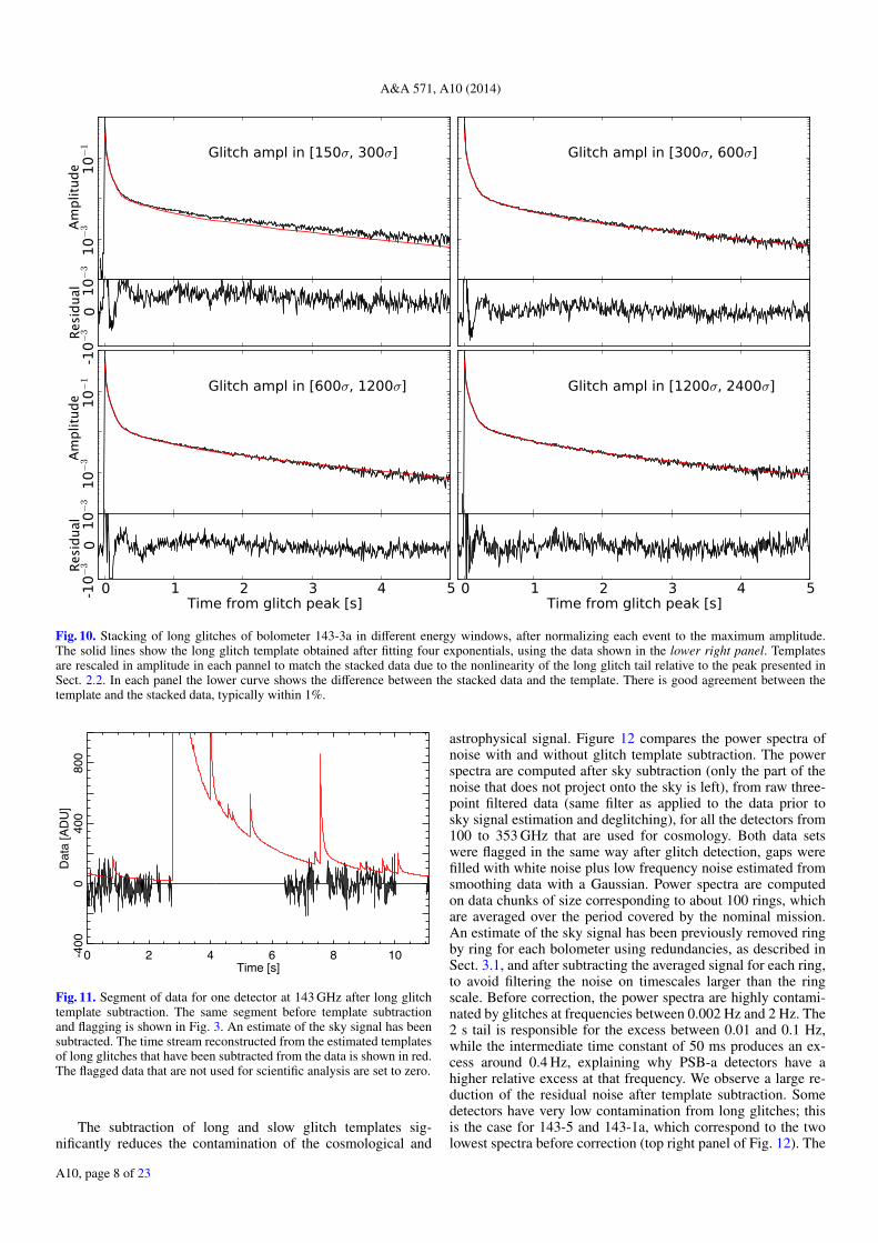
Long and short glitch templates, built from a sum of exponen-tials, are fitted to stacked (normalized and averaged) large ampli-tude events (typically 1000 times the rms noise). Any representa-tion of the glitch pulses providing a good fit to the stacked glitchdata would have been convenient for the analysis. However, thefunctional form is motivated by very simple physical thermalmodels of the bolometer and its environment. Time series are notused directly because of noise contribution to the long tail whichis filtered by the model. The stacked data are produced using themedian value for each bin corresponding to the sampling periodindex after the maximum. The median is used to avoid signifi-cant contribution from other glitches. Figure 10 shows the differ-ence between long glitch stacks and the best-fit template (withfour exponentials) in different energy windows for one bolome-ter (143-3a). The glitch template is determined using events withamplitudes between 1200 and 2400σ.

The difference between the stacked glitch data and the fit-ted template is small, but not consistent with zero, reflecting thelimit of the summed exponential model. The difference is sys-tematic, has a low frequency component, and is about 1% of thetemplate, which is much smaller than the fitting errors in eachindividual glitch described in Sect. 4.2.2 (see Fig. 16 in partic-ular). We therefore expect that the impact of this inaccuracy onthe final results is negligible. We see no evidence for significantvariations of the shape of the template with the amplitude of theglitch, over a wide range of amplitudes: the difference betweenthe glitch template and the stacks computed over different rangesof glitch amplitude, between 300 and 5000σ (after correcting forthe nonlinearity of the glitch tail amplitude relative to the peakdescribed in Sect. 2.2), is no larger than in the amplitude range of1200–2400σ where the template is fitted. The template used forthe analysis has been estimated for a limited range of energies toavoid mismatch due to the nonlinearity effects.

For small glitches, with amplitudes <300σ, there is a non-negligible difference between the stacked glitches and the fit-ted template. This is attributed to strong selection biases, e.g.,Eddington-type bias, which affects the stacked signal, and notto real variations of the glitch template. This bias is clearly ob-served for stacked samples, showing a difference in the mean off-set before the events compared with after the events (measureda few tenths of a second later, when the glitch tail is negligible).This bias is expected to be small for the high-amplitude eventsused for modelling the templates.

3.2. Results

The fraction of the data that are found to be contaminated byglitches and are ignored in the analysis varies from 6% (fordetectors with fewer long glitches) to 20%, depending on thebolometer. The averaged fraction of flagged data by HFI fre-quency is 14.4, 16.1, 16.8, 17.1, 12.8, and 11.2%, for 100to 857 GHz. Figure 11 shows a segment of data for a bolometerwith a high glitch rate after glitch template subtraction. This isthe same segment as shown in Fig. 3 before deglitching. It showsclearly that the template subtraction is very effective.

A10, page 7 of 23

A&A 571, A10 (2014)

Text

Residual

Residual

Amplitude

Amplitude

Fig. 10. Stacking of long glitches of bolometer 143-3a in different energy windows, after normalizing each event to the maximum amplitude.The solid lines show the long glitch template obtained after fitting four exponentials, using the data shown in the lower right panel. Templatesare rescaled in amplitude in each pannel to match the stacked data due to the nonlinearity of the long glitch tail relative to the peak presented inSect. 2.2. In each panel the lower curve shows the difference between the stacked data and the template. There is good agreement between thetemplate and the stacked data, typically within 1%.

-4

00

040

080

0

0 2 4 6 8 10Time [s]

Dat

a [A

DU

]

Fig. 11. Segment of data for one detector at 143 GHz after long glitchtemplate subtraction. The same segment before template subtractionand flagging is shown in Fig. 3. An estimate of the sky signal has beensubtracted. The time stream reconstructed from the estimated templatesof long glitches that have been subtracted from the data is shown in red.The flagged data that are not used for scientific analysis are set to zero.

The subtraction of long and slow glitch templates sig-nificantly reduces the contamination of the cosmological and

astrophysical signal. Figure 12 compares the power spectra ofnoise with and without glitch template subtraction. The powerspectra are computed after sky subtraction (only the part of thenoise that does not project onto the sky is left), from raw three-point filtered data (same filter as applied to the data prior tosky signal estimation and deglitching), for all the detectors from100 to 353 GHz that are used for cosmology. Both data setswere flagged in the same way after glitch detection, gaps werefilled with white noise plus low frequency noise estimated fromsmoothing data with a Gaussian. Power spectra are computedon data chunks of size corresponding to about 100 rings, whichare averaged over the period covered by the nominal mission.An estimate of the sky signal has been previously removed ringby ring for each bolometer using redundancies, as described inSect. 3.1, and after subtracting the averaged signal for each ring,to avoid filtering the noise on timescales larger than the ringscale. Before correction, the power spectra are highly contami-nated by glitches at frequencies between 0.002 Hz and 2 Hz. The2 s tail is responsible for the excess between 0.01 and 0.1 Hz,while the intermediate time constant of 50 ms produces an ex-cess around 0.4 Hz, explaining why PSB-a detectors have ahigher relative excess at that frequency. We observe a large re-duction of the residual noise after template subtraction. Somedetectors have very low contamination from long glitches; thisis the case for 143-5 and 143-1a, which correspond to the twolowest spectra before correction (top right panel of Fig. 12). The

A10, page 8 of 23

Planck Collaboration: Planck 2013 results. X.

10

-110

010

110

210

3

10-3 10-2 10-1 100 101

Frequency (Hz)

Noi

se p

ower

spe

ctra

(arb

itrar

y un

its)

100 GHz

10

-110

010

110

210

3

10-3 10-2 10-1 100 101

Frequency (Hz)

Noi

se p

ower

spe

ctra

(arb

itrar

y un

its)

143 GHz

10

-110

010

110

210

3

10-3 10-2 10-1 100 101

Frequency (Hz)

Noi

se p

ower

spe

ctra

(arb

itrar

y un

its)

217 GHz

10

-110

010

110

210

3

10-3 10-2 10-1 100 101

Frequency (Hz)

Noi

se p

ower

spe

ctra

(arb

itrar

y un

its)

353 GHz

Fig. 12. Power spectra of the component of noise that does not project onto the sky, for each bolometer at frequencies between 100 GHz (topleft panel) and 353 GHz (bottom right panel). Black curves correspond to the power spectra without subtraction of templates for PSB-b andSWB detectors, while the blue curves are for PSB-a detectors. Power spectra are rescaled in amplitude so that they all match at 20 Hz. The redcurves are with template subtraction. Power spectra are computed over subsets of about 100 rings and are averaged over the nominal mission. Thesky signal has been previously subtracted from the data. This creates the narrow dips in the spectra at the harmonics of the spin frequency. Datahave also been three-point filtered and flagged after glitch detection. The large spikes in the spectra, unsubtracted at this stage, are induced bythe 4 K J-T cooler and are described in Planck Collaboration VI (2014). The roll-off of the spectra above 10 Hz is mainly due to the three-pointfilter. Glitches contribute to the power spectra between 0.002 Hz and 2 Hz. The power spectra of residual contamination is significantly reducedafter glitch template subtraction, at frequencies below a few hertz. There is much less dispersion between the power spectra from different detectorsafter correction – less than a factor of two – indicating that contamination from remaining glitches is not a dominant effect.

improvement after deglitching is effective but small for these de-tectors, as expected, and their corrected power spectra are veryclose to the fundamental limit of the noise. The power spectrafor these detectors are then indicative of the power spectra ofnoise without glitches.The power spectra for the other detec-tors approach this limit after template subtraction. Noting thatthe 1/ f part of the spectrum varies in amplitude from bolome-ter to bolometer, we conclude that residual contamination fromglitches is below the noise level at all scales for all detectors.

One and only one of the 100 GHz bolometers (100-1a) has anextra family of glitches that are not properly accounted for by ourdeglitching method. Some of these events are detected as “long”in the processing, and then the long glitch template is incorrectlysubtracted (those events are shorter than the long events). But thematched filter, designed to detect long glitch tails (either posi-tive or negative) allows us to flag segments of data when thishappens, limiting the effect. This bolometer is the one with thelargest excess noise power at frequencies around 0.1 Hz. Thisis still a small effect, which is accounted for in the total noisebudget (Planck Collaboration VI 2014).

The power spectra of noise after sky subtraction are indica-tive of the quality of the glitch correction, but cannot be used

to derive accurately the contribution to the maps. The reason isthat part of the noise is filtered due to the “noisy” estimationof templates by the fitting procedure, which are then removedfrom the data. This is not the case for the signal projecting ontothe sky, since the method iterates between sky signal and glitchdetection, and then template fitting and subtraction. The contri-bution of glitches to the total power after data reduction at themap level, and at the ring level, can be studied with simulations(Sect. 4).

As we will see in Sect. 5.4, long glitches occur simul-taneously in both bolometers of a PSB pair. Consequently,glitches below the detection threshold, or any unsubtracted tails,are expected to induce residual additional correlations betweenbolometer time streams from the same pair. In order to evalu-ate the contribution from residual glitches we have computedthe cross-power spectra between bolometers. These are shownin Fig. 13 for detectors at 100 GHz, after averaging cross-and auto-power spectra computed on data segments of about100 rings over the entire nominal mission. The sky signal hasbeen removed and data have been processed in the same wayas previously described for auto-spectra. Bolometers from thesame PSB pair have an extra correlation above 0.2 Hz, which

A10, page 9 of 23

A&A 571, A10 (2014)

10

-410

-210

010

2

10-3 10-2 10-1 100 101

Frequency (Hz)

Noi

se p

ower

spe

ctra

(arb

itrar

y un

its)

Fig. 13. Cross- and auto-power spectra between detectors at 100 GHz.Spectra are computed in the same way as described in the caption ofFig. 12. Black curves correspond to some of the auto-spectra shownin the same figure. Data have been rescaled so that auto-spectra matchat 20 Hz, and so that the white noise level is approximately unity. Bluecurves correspond to cross-spectra between detectors from the samepair. Red curves are for detectors from different pairs. The extra corre-lation observed for PSB pair bolometers, above 0.1 Hz and at the levelof 2 to 7% of the white noise spectrum, is due to residual glitches be-low the threshold. Some residual correlation at the level of about 0.1%at 0.2 Hz can be seen between other bolometer pairs that are spatiallyclose to each other; this might result from imperfect sky signal subtrac-tion due to pointing drift, since the error is coherent between differentnearby detectors. The low frequency noise is highly correlated betweendetectors and is due to thermal fluctuations of the focal plane. The levelof correlation of the 4 K lines in the plot is not representative of theresidual obtained after the TOI processing.

is around 2–7% of the white noise level in the spectrum for100 GHz bolometers. The correlation is 2–3% for PSB pairs at143 GHz, 1–4% at 217 GHz, and 2–4% at 353 GHz. Simulationspresented in the next section show that the residual noise excessis of the order of 5% (Fig. 16); given our modelling of glitches(Sect. 5.4), and noting that about half of the glitches have thesame amplitude in PSB-a and PSB-b detectors (see Sect. 5.4),we should have roughly 5% correlation in the noise spectrum.This is slightly higher than the 3% observed for this pair. Thedifference could be due to uncertainties in our modelling andmodel extrapolations. It is important to note that we observestronger correlations in pairs for which both detectors have fewdetected long glitches, e.g., the 100-4a/4b pair, for which thedetectors have the lowest glitch rates (as shown in Fig. 9), andwhich have 7% cross-correlation (as seen in Fig. 13), the high-est observed for any pair. This is entirely explained by the factthat both detectors then have more glitches below the detectionthreshold, since the counts for long glitches are similar betweendetectors, but are essentially scaled in energy, as described inSect. 5.4. By contrast, pairs for which the faint-end break incounts is above the detection threshold have significantly lowercorrelations above 0.1 Hz.

We have shown that glitches below the detection thresholdare responsible for the extra correlation in the noise by averagingthe two time streams from each pair of bolometers, and lookingfor events above 3.2σ (of the noise) in the combined data. Thisallows us to detect coincident glitches with amplitudes lower bya factor of

√2 for about half of the events, enabling us to di-

vide the correlated noise by a factor of 2, with only 0.1% ofadditional data flagging. This shows, without ambiguity, that the

extra correlation between two bolometers in PSB pairs is due toundetected long glitches below the threshold.

Furthermore, this analysis confirms that the number of un-detected glitches is small and that a change in slope (or break)must happen in the counts close to the detection threshold, as wewould otherwise have expected more correlations in the noisebetween PSB pairs. Those glitches then account for a smallfraction of the total noise power.

4. Impact of glitch residuals on final results

4.1. Simulations

In order to estimate the contamination from glitches that remainsafter processing, we have performed simulations of glitch timestreams, incorporating the glitch properties that we measure indata. The simulations include the following features.

– Glitches are generated using a Poisson distribution, with sub-sample resolution.

– Generated glitches follow the population spectra that arefound in data for each population by combining bolometers,and using the model explained in Sect. 5. Population spec-tra are rescaled in energy for each bolometer to match themeasured counts. In particular, we use to build the modelthe measured number counts of long glitches in the submil-limetre channels because those channel are more sensitive tolow-energy glitches, below the faint-end break. Populationspectra of short and slow glitches are extrapolated at lowenergy (for which events can not be detected individually)using power laws.

– The nonlinearity of the slow tail of long glitches relative tothe peak amplitude is included (see Sect. 2.2 for details).

– The temporal shape of glitches is simulated using templatesfor the slow parts (after about 20 ms), analytically correct-ing the effect of the sampling average and of the three-point filter on the amplitude of the exponentials, since thoseare applied to the data before template estimation. The fastpart of glitches is simulated using subsample resolution, andthen averaged over the sample period with a simple boxcaraverage.

The simulations do not include the apparent scatter of the slowtail amplitude of long glitches, apart from the intrinsic scatterdue to the variations of the arrival time in the sample period.Those fluctuations do not strongly affect the performance of themethod, since the slow part of the glitches is fitted before sub-traction, and so the amplitude variations are absorbed by the fit.Moreover, we used a fixed template for short glitches, whichis not completely realistic, since we have observed scatter inthe slow tail, and we have identified two subcategories of shortglitches. The effect of using a single, fixed template for shortglitches should be very small, since the short glitch templatesare not removed. We did not include the 2 s exponential decayfor short glitches in the simulations, since the uncertainty in itsamplitude is large. Nevertheless, we estimate that the contribu-tion to the power spectrum should be below 0.1% of the noisepower spectrum, given the distribution of short glitches. The ef-fects of nonlinearity of the bolometers and the ADC are not sim-ulated. The nonlinearity has the effect of reducing the fast partof the glitches, which dominates at very high amplitudes. Wedo not expect this to degrade the performance of the method forthe slow part of the glitches, since the template fitting starts afew samples after the peak, in a part of the signal that is not

A10, page 10 of 23

Planck Collaboration: Planck 2013 results. X.

10-6

10-4

10-2

100

102

104

101 102 103 104

Amplitude (signal to noise)

Num

ber

of e

vent

s / n

oise

rm

s/ h

our

TotalLongShortSlow

143-2a

Fig. 14. Differential counts for the three populations of glitches for oneof the detectors with a high rate of glitches (143-2a) measured fromsimulated data. This can be compared to the results on real data shownin Fig. 8 for the same bolometer. Dashed lines are shown for referenceand are identical to the lines shown for the real data. There is almostperfect agreement between simulations and data, except for very highamplitude glitches >∼104σ. Those glitches are affected by the bolometernonlinearity in the real data, an effect that we did not simulate at thisstage, explaining the discrepancies in the counts. We simulated slightlyfewer very high amplitude slow glitches than in the Planck data. Thisaffects only about one event per day.

affected by nonlinearity. Finally, we do not include the corre-lation of glitches between PSB pairs, but treat each bolometerindependently.

To the generated glitch signal, we add Gaussian noise con-taining a white component and a low frequency component de-scribed by a power law fitted to the data (with an index and fkneeparameter). We also add a time stream of pure signal obtainedby scanning over a simulated cosmic microwave background(CMB) map, as well as Galactic dust and point source mapsfrom the Planck Sky Model (Delabrouille et al. 2013), usingthe pointing solution derived for the actual data. The constructedsignal time stream is formed by interpolating the extracted sig-nal from the map to limit subpixel effects (see Reinecke et al.2006, for the methodology). We also filter the simulated datausing the same three-point filter as used for the data. The dif-ferential counts recovered from the simulations after processingare shown in Fig. 14 for bolometer 143-2a. There is very goodagreement with the spectra recovered in Planck bolometer data,shown in Fig. 8.

4.2. Error estimation

4.2.1. Evaluation of signal bias due to the deglitchingprocedure

Due to the high signal-to-noise ratio of HFI data, the sky signalsubtraction is a critical part of the deglitching procedure. Errorsin the sky signal estimation could easily induce spurious detec-tion of glitches and errors in the template subtraction, whichwould then correlate with the signal. This could bias the sky sig-nal estimation for two main reasons: first by flagging data as badslightly more often on average when the sky signal is higher (orlower); and second, by subtracting slightly more glitch templatesignals when the fluctuations of the sky signal are of a givensign.

We have verified the absence of bias in the signal with thehelp of simulations. Specifically, we have computed signal rings

by projecting pure signal time streams used for simulations,which we write as r0i(p), where p is the ring pixel and i is thering number. We have also projected the simulated observed datafrom which we have subtracted estimated glitch templates, afterapplying the deglitching procedure used for real data and reject-ing flagged data. We write this last quantity as r̂i(p) for dataring i. We then computed the average binned power spectrumof r0i(p) as:

P0(q) =1

NNq

N∑i=1

∑k∈Dq

r0i(k) r0i(k)†, (1)

where † denotes the transpose conjugate, r0i(k) is the Fouriertransform of r0i(p), Dq and Nq are the intervals in k and the num-ber of modes in bin q, respectively, and we have summed overN rings (with N of the order of 10 000). We also computed theaverage cross-power spectrum between r0i(p) and r̂i(p) as

Pc(q) =1

NNq

N∑i=1

∑k∈Dq

r0i(k) r̂i(k)†. (2)

In the absence of bias in the signal introduced by any of thetwo effects previously described, Pc(q) should be an unbiasedestimate of P0(q), i.e.,

P0(q) = 〈Pc(q)〉 , (3)

where 〈·〉 is the ensemble average over an infinite number ofrealizations of noise and glitches.

In practice, the quantities P0(q) and Pc(q) − P0(q) are evalu-ated for simulations of the 143-2a detector for N = 10 000 rings.We selected rings with no strong Galactic signal, to avoid giv-ing too much weight to the Galaxy, keeping about 95% of therings. Results are shown in Fig. 15 for logarithmically spacedbins. We can see that Pc(q)−P0(q) is compatible with zero at allscales. We estimate an upper limit to the bias of around 5× 10−4

in individual bins at all scales relevant for cosmology, i.e., fork corresponding to 1 ≤ ` ≤ 2000. The absence of significantbias due to the deglitching procedure is verified at the ring level,but this conclusion can be drawn at the map level, and hence atthe CMB power spectrum level. Also, we do not expect to ob-serve differences for the CMB measured with other bolometers,since the presence of bias has to do with the errors made in thesky signal reconstruction, and not on errors made in glitch tem-plate fitting and subtraction. Nevertheless, we have performedthe same exercise for an SWB bolometer at 143 GHz (143-5).We did not find any bias and can place an even lower limit of2 × 10−4, due to the lower rate of glitches for this bolometer.

The situation is different for strong Galactic signals and forhigh frequency channels, since the detection threshold is in-creased with the signal amplitude and even long glitch tem-plates are not subtracted for very high sky signal, as described inSect. 3.1. We expect this to slightly bias the estimation of the skysignal in the positive direction, since less positive glitch signal isremoved in regions of strong sky signal. This effect is describedin detail in Planck HFI Core Team (2011b). In particular we ob-served an effect of the order of 4 × 10−4 of the signal amplitudeat 545 GHz. The effect on the beam response estimation is stud-ied in detail in Planck Collaboration VII (2014).

Because the sky signal is estimated using data from indi-vidual rings, the estimate is noisy, with an rms that is reducedby roughly a factor of 7 compared to the rms of the noise ineach measurement. This induces some weak correlations in theglitch detection between each circle in the ring, after the sky sig-nal has been removed from the data. However, this effect does

A10, page 11 of 23

A&A 571, A10 (2014)

10

-810

-710

-610

-510

-410

-3

10-4 10-3 10-2 10-1

k [arcmin-1]

k2 P(k

) (ar

bitra

ry u

nits

)

Fig. 15. Constraints on the signal bias after deglitching. The black curveis the power spectrum (k2P0(k), with k taken at the centre of each bin q)of ring data after projecting a pure simulated signal time stream for onedetector, containing CMB anisotropies, Galactic dust and point sourcesignal, and using the actual pointing. For the other displayed points wecomputed the cross-spectrum between: (1) the estimated signal on ringsafter subtracting long glitch templates from the simulated data and af-ter flagging; and (2) the input signal only averaged on the same rings.Crosses and diamonds correspond to the difference between this cross-spectrum and the pure input signal power spectrum shown in black,for positive and negative points, respectively. The quantity displayedis k2(Pc(k) − P0(k)). We averaged the power spectra of 10 000 rings.Simulations were performed for detector 143-2a which has a high glitchrate. In the absence of bias in the signal due to the deglitching, we ex-pect that the cross-power spectrum is an unbiased estimator of the inputsignal power spectra, and that the difference should then be compatiblewith zero. We do not detect significant bias in any of the 100 logarith-mically spaced bins, and we place an upper limit of 5 × 10−4 on eachbin at the scales relevant for CMB analysis.

not bias the estimation of the signal, as shown above, but corre-lates slightly, at the level of 1%, with the remaining noise (afterflagging and template subtraction) between subsets of data mea-sured by taking half rings. We have studied this effect in PlanckCollaboration VI (2014, see Table 2 and Fig. 32) and it has beentaken into account for the noise prediction.

4.2.2. Residual glitch contamination

For some representative bolometers we have evaluated the levelof contamination coming from glitches left in the data after pro-cessing at the ring level, by comparing the power spectrum of theinput simulated noise projected on rings with the power spec-trum of processed simulated data, after removing the input skysignal from the data. This is shown in Fig. 16 for simulationsof data from the same two detectors as in the previous section:143-2a, containing a high rate of long glitches; and 143-5, with alow glitch rate, but consequently more glitches below the thresh-old (see Sect. 5.4), after averaging the spectra over 10 000 rings.We also compare these two power spectra with the power spec-tra obtained without removing glitch templates from the data,but using the same data flagging.

For bolometer 143-2a, we can see that without templatesubtraction the glitch signal dominates over the noise on largescales, k < 2 × 10−3 arcmin−1, even after flagging. We ob-serve a dramatic improvement in the noise power spectrum af-ter removing long glitch templates. Nevertheless, glitch resid-uals still contribute to the noise power at the level of 30%

at k . 2 × 10−3 arcmin−1 and less than 10% at k & 6 ×10−3 arcmin−1. We attribute the excess at low frequency to errorsin the subtraction of templates, which are expected to arise dueto uncertainties in the amplitude parameter determination afterχ2 minimization. Given the level of residuals in power spectra,the impact of errors in template estimation is negligible at thepercent level, as seen in Sect. 3.1.4. Undetected glitches belowthe threshold contribute significantly at higher frequencies, atthe level of 5% of the power for this bolometer, and cause theobserved excess over 0.03 < k < 0.1 arcmin−1. For bolome-ter 143-5, the contamination by glitches before template sub-traction below k < 10−3 arcmin−1 is between 15 and 20% and ofthe order of 8% above 10−3 arcmin−1. After glitch template sub-traction, the contamination reaches the level of 8% for almostall scales. This value corresponds to the level of contaminationby undetected glitches below the threshold, which is higher thanfor the 143-2a bolometer, in agreement with our modelling (seeSect. 5.4).

This study shows that the remaining contamination fromglitches is below the instrumental noise level, even for the chan-nels with the highest glitch rates. Evaluation of the contamina-tion at the map level and its effect on the CMB power spectrumis postponed until the release of the data for the full Planck mis-sion. Nevertheless, the contribution of glitches to the errors oncosmological results (Planck Collaboration XVI 2014; PlanckCollaboration XV 2014) has already been accounted for, sincethe noise estimation is based on differences of half-ring periods(Planck Collaboration VI 2014).

5. Glitch characterization and interpretation

In this section we focus on a more detailed description of thecharacteristics of the different glitch types and provide an inter-pretation of their origin. This analysis is complementary to thestudy based on ground tests presented in Catalano et al. (2014).

5.1. Evolution of the glitch rate over the mission

Over the course of the whole mission, the rates of each typeof glitch decreased (Fig. 17). This decrease is universal for allbolometers (Fig. 9). The signal from diode sensor TC2, the mostshielded of the three diodes in the standard radiation event mon-itor (SREM, Mohammadzadeh et al. 2003) located on the Sunside of the Planck spacecraft, follows a similar trend with time(Fig. 18). This trend is expected for Galactic cosmic rays mod-ulated by the heliosphere of the Sun (Gleeson & Axford 1968;Bobik et al. 2012) and is observed by ground stations on Earthand other spacecraft in the solar system (Usokin et al. 2011;Wiedenbeck et al. 2005; Adriana 2011). Taking together theglitch rate, the SREM diode signal, and data from other stud-ies, it is clear that the source of glitches in the HFI bolometers isdominated by Galactic cosmic rays. Indeed, other sources, suchas on-board radioactivity and solar protons (as detected by themirror on WMAP, Jarosik et al. 2007), were suspected to con-tribute to the glitch rate, but would not follow the trends withtime that are observed.

5.2. Correlation in time

The time interval between two consecutive glitch events exhibitsan exponential distribution (left panel of Fig. 19). The absolutevalue of the slope fitted between 1 and 2 min is roughly equalto the computed rate, simply obtained as the number of events

A10, page 12 of 23

Planck Collaboration: Planck 2013 results. X.

10

010

1

10-4 10-3 10-2 10-1

k [arcmin-1]

Rin

g no

ise

P(k)

(arb

itrar

y un

its) 143-2a

10

010

1

10-4 10-3 10-2 10-1

k [arcmin-1]

Rin

g no

ise

P(k)

(arb

itrar

y un

its) 143-5

Fig. 16. Estimation of the power spectra of noise residuals after averaging data on rings for the 143-2a bolometer (left) and the 143-5 bolometer(right). Power spectra are averaged over 10 000 rings and are computed after removing the input simulated signal from the simulated data andusing the estimated flags. The dot-dashed curve is the result without subtraction of long glitch tails, while the solid curve is with subtraction asdone for the real data, and the dashed curve is for the same simulations but without glitches. Residual glitches are significantly reduced aftertemplate subtraction.

Fig. 17. Mean rate of the three categories of glitches, i.e., long, short,and slow. These rates are computed using all 52 bolometers for long andshort glitches, and the 16 PSB-a bolometers for slow glitches.

above 10σ in six months (right panel of Fig. 19). Clearly, all thebolometer glitch distributions exhibit Poisson behaviour. Theseparticular data are from Survey 3 when the glitch rate was rela-tively constant and events above 10σ were selected to avoid anycontamination by false events, solar flares, and pile-up. We can-not check multiple simultaneous events because we cannot dis-tinguish between a pile-up of multiple events and a single moreenergetic event. Still, the glitch data are compatible with purerandom events that are not correlated in time and this is consis-tent with the cause of events being individual hits by Galacticcosmic ray particles.

We also studied the coincidence of events between bolome-ters. We found that the largest fraction of coincidences,around 99%, are between PSB-a and PSB-b detector pairs in thesame module (see below). The remaining roughly 1% of coinci-dences are particle shower events that effect a large fraction ofthe detectors in the focal plane in different modules (the showerevents will be discussed in Sect. 5.7).

Fig. 18. Top: normalized glitch rate (black line), cosmic ray flux mea-sured by the SREM for deposited energy E > 3 MeV (purple), and E >0.085 MeV (pink), as a function of time. Bottom: monthly smoothednumber of sunspots.

5.3. Interaction with the grid/thermistors

There is clear evidence that the short events result from cosmicrays hitting the grid or the thermistor. Indeed, these events havea fast rise time and have a fast decay, and the transfer functionbuilt from the short glitch template (see Catalano et al. 2014, fora comparison) is in good agreement with the HFI optical transferfunction (Planck Collaboration VII 2014), so the energy must bedeposited in the environment close to the thermistor. Figure 20shows the cumulative counts, i.e., the number of events N(>E)with an amplitude higher than a given value E per hour, for shortglitches, after converting the maximum amplitude of each glitchto units of energy (keV) for one reference bolometer (100-1b).The energy calibration for the other bolometers has been scaledso that the cumulative distributions match the one for the refer-ence bolometer at energies of about 10 keV. For this conversionwe use the measured heat capacity of the NTD crystal plus gridsystem (see Holmes et al. 2008), since we assume that the energyof the events is deposited in this system. The relative fitting ofthe energy is necessary for the comparison between bolometers

A10, page 13 of 23

A&A 571, A10 (2014)

Fig. 19. Left: time interval between two consecutive glitch events for each bolometer, normalized by the total number of events. Colours distinguishdifferent detectors. We observe Poisson distributions, as expected for random events. Right: glitch rate derived from the slope of the time intervaldistribution, compared to the mission averaged actual rate for each bolometer.

10

-310

-110

110

3

10-2 10-1 100 101 102

Amplitude [keV]

Num

ber o

f eve

nts

N(>

E) p

er h

our Short (nonlinearity corrected)

LongSlowTotal

Fig. 20. Cumulative counts (per hour) for the three categories of glitchesand for several bolometers: blue curves are for short glitches after non-linearity correction above typically 10 keV (as described in the text);black curves are for long glitches; red curves are for slow glitches; andgreen curves are for the total counts without the nonlinearity correction(which is why they lie below the blue curves). Glitches are not separatedinto the different categories below 10 times the rms noise (i.e., about20 eV). All curves have been recalibrated in energy for each bolometer,such that the distributions of short glitches match at energies around10 keV (we use the same coefficient for all populations), the absolutecalibration being fixed for one arbitrary detector. Note that the distribu-tions of short glitch match very well, while there is a large scatter in theenergy scaling for the other populations of glitches.

because of uncertainties in the heat capacity of the system, andalso in how much the peak amplitude is reduced after averagingover the interval of one sample within the electronics. Peak am-plitude reduction is more important for faster bolometers. Theeffect is significant for the submillimetre channels, for which thetime constant is very small. We determined that the relative cor-rection factor should be about 3 for 100–545 GHz bolometers.We have also reconstructed and corrected the counts for highamplitudes that are affected by nonlinearity (typically above10 keV) by readjusting the values of event energies using themeasurements of the slow tails of short events (which are notaffected by nonlinearity since they are too low in amplitude), in-stead of directly taking the peak amplitude. This allows us to

reconstruct the distribution more than a factor of ten above thesaturation level set by the electronics. We can see in Fig. 20 thatthe counts of short events for all detectors match fairly well (con-sidering the fact that no rescaling is performed on the y-axis, butonly in energy), particularly around the energy bump.

Events in the bump are expected to be associated withcosmic rays hitting the thermistor. Since the thermistors areidentical for all bolometers, we expect the same rates for allbolometers, which is precisely what we observe (Fig. 20).Given the dimensions of the thermistors of 30 µm × 144 µm ×341 µm, and the fact that typical Galactic protons of energiesaround 1 GeV (the peak of the spectrum) deposit minimum en-ergies of ≈1.47 MeV cm2 g−1 in the Ge (which is the minimumof the stopping power for normal incidence in the largest sur-face), we expect typical deposition energies of 15 keV in thethermistor (the first energy being dominant, since it correspondsto the largest cross-section). This is also in agreement with theenergy measured experimentally, given that the energy calibra-tion is uncertain within about 50%. The amplitude of the bumpin the cumulative distribution, which is at about 10 events perhour, also matches with the expectations. Indeed, by integratingthe expected cosmic ray spectrum at L2, and considering thatlow energy particles are absorbed by the spacecraft, we can pre-dict a total particle rate of N ≈ 5 s−1 cm−2. This leads to a glitchrate of about 8 h−1 on the thermistor.

The events depositing an energy of about 10 eV to 1 keV andpopulating the power law seen in Fig. 20 are expected to be theresult of cosmic rays hitting the grid. Calculations predict a totalrate of events on the grid from 7 to 90 h−1, given that the surfacearea of the grid varies from 4.77 × 105 µm2 to 3.95 × 104 µm2,depending on the bolometer. We observe a higher number ofevents, by a factor of 2–4, but (as we will see in the next para-graph) about half of the events for PSB bolometers might resultfrom electrons ejected from the other grid by the impact of a cos-mic ray proton. We observe some dispersion in the amplitudes ofthe power-law distributions from bolometer to bolometer, whichis not obviously correlated with the area of the grids. This is at-tributed to the uncertainties in the intercalibration of energy tomatch the counts, as detailed at the beginning of this section.

We have performed a coincidence analysis of short eventsbetween PSB pairs. At the arrival time of each short glitch de-tected in a PSB-a bolometer, we have measured the level of

A10, page 14 of 23

Planck Collaboration: Planck 2013 results. X.

Fig. 21. Representative short glitch coincidences in a PSB pair. Thex-axis represents the amplitude relative to the noise of the detectedglitch in the PSB-a bolometer, while the y-axis is the value of the signal-to-noise ratio in the PSB-b bolometer. The grey-scale indicates the logof the number of events in logarithmic bins. Detected events are notshown below 100σ in PSB-a, as we expect a non-negligible contributionfrom long glitches, and the separation between long and short glitchesis uncertain at low amplitudes. A large fraction of events are coincidentbetween PSB-a and PSB-b.

signal in the PSB-b detector in the same module. We comparethe amplitude of the signal in the PSB-b (without regard to thecategory of the signal in the PSB-b) with the amplitude of theglitch at its maximum in the PSB-a, and computed a 2D his-togram of the two quantities. The 2D distribution of amplitudesfor short glitches in the PSB-a is shown in Fig. 21. The eventsbelow 100σ are not displayed since the separation between shortand long glitches is then uncertain. We observe that the distribu-tion is very different from the expected distribution for randomcoincidence. The expected distribution of amplitudes for randomcoincidences is evaluated by measuring the statistics of the sig-nal in the PSB-b at a time 10 000 samples (about one minute,i.e., well after a short glitch has terminated) after each event inthe PSB-a, and this is shown in Fig. 22. In particular, we can seea wide cloud of points in the 2D histogram above about 10σ inPSB-b. A fraction of around 50% of the events populate the re-gion of random coincidence. This is also shown in Fig. 23, whichdisplays the distribution of the signal in the PSB-b for events inthe PSB-a with amplitudes between 300 and 1000σ. So thereare strong indications that about 50% of short glitches are seenin coincidence between PSB-a and b. However, for a given am-plitude of short glitch in PSB-a, we observe a wide distributionof amplitudes in PSB-b. We have verified that counterparts inPSB-b have no phase shift.

A possible model for these coincidences is that events hit-ting one of the grids eject some electrons which hit the othergrid. The rate of 50% correlation can be explained by geomet-rical effects, such as particles coming from the top or bottom;a particle coming from the top could hit the PSB-a grid, extractelectrons, and project those onto the PSB-b grid, whereas a par-ticle coming from the bottom and hitting the PSB-a grid wouldnot project electrons onto the PSB-b. The observations indicate,

Fig. 22. Expected distribution for random coincidences, for comparisonwith Fig. 21. The value of the signal-to-noise ratio in PSB-b for eachshort event in PSB-a is taken 10 000 samples afterwards. We use shortevents in PSB-a so that this distribution can be directly compared to thecoincidence of short glitches.

10

-110

010

110

210

310

4

0 20 40 60 80 Signal to noise 143-4b

Num

ber o

f eve

nts

Fig. 23. Distributions of the signal values in PSB-b for short events withpeak amplitudes between 300 and 1000σ in PSB-a (solid line). A ran-dom distribution of values in PSB-b is also shown (dot-dashed line).The excess of the solid curve over the dot-dashed curve for amplitudesabove 3σ represents about 50% of the total area. Thus, at least 50% per-cent of the events are in coincidence between PSB-a and PSB-b.

then, that nearly all events hitting one of the grids and comingfrom the appropriate direction must eject electrons hitting thesecond grid and deposit about 10% of the energy deposited inthe first grid. We also observe that some events clearly hit bothgrids. These appear in the cloud of points (in Fig. 21) with thesame amplitude in both the PSB-a and b, representing about 2%of the events. We observe a lower coincidence rate for eventsat higher amplitudes corresponding to the bump. This is ex-plained by the hypothesis that those events correspond to directimpacts on the thermistor, which is not aligned with the grid ofthe other bolometer. Nevertheless, we have seen that all thosehigh energy events are in coincidence with a small amplitudeevent in the second bolometer. This is attributed to the cross-talk

A10, page 15 of 23

A&A 571, A10 (2014)

between bolometers in a pair, as discussed in Sect. 5.5. The non-linearity, appearing as the curved shape in the coincidences, canbe entirely explained by the saturation of the highest amplitudeglitches. Nevertheless, we can evaluate the level of cross-talk tobe between 0.01 and 0.44%, depending on the bolometer pair,for about 3000σ events (for which the effect of saturation issmall). The high amplitude events correspond to an energy of≈15 keV left on the grid+thermistor by a particle; this is veryclose to the expected energy deposited by a 1 GeV proton ontothe thermistor.

5.4. Interaction with the wafer

We identify the long glitches as being produced by cosmic rayshitting the silicon die. This was first indicated by the groundtests (Catalano et al. 2014), showing that the NTD thermome-ter is sensitive to a temperature change of the Si die. The HFIground-based calibration data show a rate of events compati-ble with the cosmic ray flux at sea level over the Si die sur-face, and the ground-based data also show that almost all theseevents are in coincidence between PSB-a and PSB-b. Our under-standing is the following. Hot carriers are generated by the par-ticle impacts on the Si die. These rapidly decay into hot ballisticphonons which cause the rapid (athermal) rise in NTD Ge tem-perature. The bolometer temperature then decays with fast op-tical time constant. The next slower time constant is due to thethermal response of the Si die (Catalano et al. 2014). The slow-est thermal response is due to the heat flow through the coppermodule and into the 100 mK heat sink (Spencer et al., in prep.)This hypothesis is reinforced by the comparison of cumulativecounts N(>E) of long glitches from bolometer to bolometer(Fig. 24). To make this comparison, we have normalized thecounts so that we are evaluating the number of events per unittime and per unit surface area of the Si wafer (because the to-tal surface varies from bolometer to bolometer). Also, as forshort glitches, we have intercalibrated the energies of events be-tween bolometers by matching the different counts at measuredenergies around 0.05 keV, which corresponds to a deposited en-ergy on the Si die of about 103 keV after absolute calibration.This absolute calibration is performed so that the observed faint-end break of the counts, which is clearly visible in the figure,matches the expected minimum energy deposited by GeV pro-tons on the Si die (which is about 140 keV, for normal incidence,as described later). This calibration of the model is necessary,since we only measure the energy in the grid+thermistor sys-tem, and the heat capacity and link conductivities are not knownwith sufficient accuracy. Additionally, we use the values of thepeaks to record the amplitudes of glitches that are not represen-tative of thermal processes, since the fast part of long glitches isexpected to result from ballistic phonon effects.

Figure 24 shows the cumulative counts for all the HFIbolometers used for the scientific analysis. We clearly see thatthey all match in shape and amplitude, with very small scatter.For energies below 20 times the rms noise, we have also com-puted the cumulative counts for all events, without distinctionbetween families (green curves in the figure); we have alreadyseen that long events dominate at low energy, so the total countsare representative of the counts of long glitches. The faint-endbreak in the counts is detected without ambiguity. This is animportant result, since it shows that there are a limited numberof undetected low energy glitches in data, which might other-wise affect the cosmological results. From this limit, we mea-sure that the total rate of events penetrating the shielding of thesatellite around the bolometers is about 4.5 s−1 cm−2. This is in

10

-410

-210

010

2

102 103 104 105 106

Amplitude [keV]

Even

t num

ber N

(>E)

per

hou

r per

mm

2

TotalLong

Toy model protonsToy model He

Toy model electrons

Fig. 24. Cumulative distribution N(>E) of long glitches per unit surfacearea of the wafer for all bolometers used for the scientific analysis. Theblack solid lines correspond to selected long glitches. The green linescorrespond to total glitches, but are representative of long glitches, sincethey dominate at low energy. We have used a relative calibration of theenergy (indicated on the x-axis) such that the cumulative counts for allbolometers match at 103 keV. The absolute calibration of the energyis set so that the faint-end break of the counts matches the expecteddeposited energy of about 140 keV in the Si die. Nevertheless, we ob-serve that the shape of the cumulative counts match for all detectors,and with a low dispersion. The break in the counts at the faint end isvery significantly detected; this is our best indication from flight datathat long glitches result from particles hitting the Si die of the bolome-ter. Dot-dashed and dashed lines correspond to the predicted power-lawdistributions of deposited energy from protons and helium, respectively,with a toy model for the interaction on the wafer using the incident par-ticle spectrum at L2 for energies significantly higher than the stoppingpower energies. Predicted minimum deposited energies for He and forprotons are indicated with dotted lines. We interpret the second appar-ent bump (seen as a slight break in the spectrum at around 20 times theenergy of the main break) as the signature of He nuclei.

good agreement with the expected value in the bolometer en-vironment computed in Sect. 5.3 of 5 s−1 cm−2. The slope andamplitude of the distribution can be predicted using a simplepower-law model of the interaction of primary Galactic protonsand He nuclei with the Si die, as shown in Fig. 24. We observea good match of the model with the data, showing that particlesdetected by Planck at the energies above the faint-end break areprimary Galactic protons. The barely apparent second bump incumulative counts at deposited energies around 3000 keV maycorrespond to the contribution from He nuclei, which are ex-pected to contribute about 10% of the counts at those energies.The fact that we observe an excess in the counts at the expectedenergy of the minimum stopping power for He reinforces ourhypothesis for the origin of long glitches. High energy Galacticelectrons could also contribute to the measured counts for highdeposited energies.

The large scatter in the distributions of long glitches with re-spect to different detectors, after calibrating the energy on theshort distributions, is shown in Fig. 20. This is due to the varia-tion of thermal links between the grid and the Si die, as well asvariations in the Si die heat capacity, reducing or increasing thefraction of energy transmitted to the thermistor for both phononsand thermal processes. The detectors with smaller glitch counts(e.g., 143-1a and 143-5 in Fig. 17) are those with a smaller frac-tion of the energy propagating from the wafer to the grid. Forthose detectors we do not see the break in the counts, sinceit should be below the detection threshold. We observe that in

A10, page 16 of 23

Planck Collaboration: Planck 2013 results. X.

Fig. 25. Representative long glitch coincidences in a PSB pair. See de-scription in Fig. 21. Events above 50σ are selected if they match thelong glitch template. All events (without selections) are included be-low 50σ, since the long glitch population dominates at low amplitudes.The solid line indicates identical signal in both the PSB-a and PSB-b.Most (if not all) long events in PSB-a are associated with significantevents in PSB-b, and a large fraction have approximately the same am-plitude in PSB-a and PSB-b.

general PSB-b detectors are more sensitive to long glitches thanPSB-a detectors (although a few exceptions exist).

Detectors with smaller rates of glitches should have moreundetected glitches than detectors with a higher rate. This hy-pothesis is verified with the help of the cross-correlation analysisbetween bolometer signals from the same PSB pair, described inSect. 3.2 (see Fig. 13 in particular). We observed that bolometerpairs with smaller glitch rates are those with higher correlationsaround 1 Hz, which is attributed to glitches below the threshold.On the other hand, pairs for which one of the bolometer has avisible faint-end break in the counts have smaller correlations inthe noise. The impact of this on final results after processing isstudied in Sect. 4.2.

We have already seen that events hitting the bolometer Si diemust deposit a fraction of their energy, which is typically theminimum stopping power of the Si for events close to normal in-cidence and with energies of 140 keV. Then, most of the eventsmust instantaneously hit the two wafers in PSB pairs. This iscompatible with what we observe by measuring the coincidenceof long events in PSB-a with signal in PSB-b, shown in Fig. 25,as we did for short events. Indeed, we find that between a thirdand a half of the events deposit the same energy in both PSB-aand PSB-b detectors, with some intrinsic dispersion, as most ofthe points lie along a line in the figure. The factor between ampli-tudes of coincident events is almost 1 in signal-to-noise units forthis PSB pair, but can vary between 0.25 and 4, depending on thebolometer pair. This factor becomes 1 after recalibrating in unitsof deposition energy on the Si die, as expected. Furthermore,100% of the events (at least for amplitudes higher that 300σ)happen in coincidence between the two bolometer pairs, but withdifferent energy deposition, by a factor of 300 at maximum. Wecannot state this for events below 300σ, since a significant frac-tion of the counterparts in PSB-b are below the noise level. We

Fig. 26. Representative slow glitch coincidences in a PSB pair. See de-scription in Fig. 21. No event is shown below 50σ, to avoid leakagefrom the long population. All slow glitches in PSB-a above about 1000σare associated with significant events in PSB-b. Below about 1000σ themajority of events are associated with significant events in PSB-b. Forthe remaining fraction the fact that we do not see a significant signalmight be simply a threshold effect.

could explain the difference in energy deposition between PSB-aand PSB-b by the fact that some relatively low energy eventslose a significant fraction of their energy in the first Si die andthen deposit more in the second, since the stopping power is adecreasing function of the energy for the considered particles.Some electrons could also be ejected from the first wafer andinteract with the second wafer (as discussed for the grid inter-action), but the associated signal would be diluted in the signalfrom the primary particle, since the events are in coincidence inthe two wafers. In principle we should have a small proportion ofevents hitting the corner of the bolometer wafer, with no counter-parts in other bolometers, but we do not have evidence for suchevents. The number of events in the distribution along the line ofone-to-one correlation is of the order of 50% of the total num-ber for events with amplitudes lower than about 300σ or aboveabout 1500σ, and is around 35% for amplitudes in between. Acomplete modelling of the interaction of particles with the twoSi dies, including accurate physical modelling of the interaction,is postponed to a forthcoming publication.

Crucially, the coincidence study indicates that the contribu-tion to the glitches by secondary particles, e.g., “delta” (or sec-ondary) electrons, is negligible, since those low energy eventswould deposit all their energy in the first wafer without acounterpart in the second.

We have also performed a coincidence analysis at the lo-cation of slow events in PSB-a. Distributions are shown inFig. 26. As already stated, slow glitches are seen only in PSB-a.Nevertheless, there is a significant signal in PSB-b associatedwith slow glitches in PSB-a. Indeed, we can see that the distribu-tion of counterparts in PSB-b is very different from the randomdistribution shown in Fig. 22, which means that slow events inPSB-a are associated with signals in PSB-b. The counterpartsgenerally have a wide range of amplitudes for a given energy

A10, page 17 of 23

A&A 571, A10 (2014)

of slow glitches, which makes it difficult to measure the associ-ated time constants. Visual inspection of those events allows usto distinguish a variety of counterparts: some have faster decaythan slow glitches and have similar rise times of around 10 ms;and some others (the larger energy ones) are similar to longglitches.

5.5. Cross-talk between bolometers

A very high amplitude short event in one of the bolometers of aPSB pair is always seen in coincidence with a small event in theother bolometer. This is attributed to cross-talk between bolome-ters. The estimated level is about 10−3, as can be seen in Fig. 21for a particular pair; the level varies between 0.01 and 0.44%for different pairs. These events show a phase shift, which variesfrom 0.25 to 1.4 samples, depending on the pair, and the trans-fer function of the cross-talk signal is different from the primaryglitch transfer function. We observe longer time constants forthe cross-talk signal than for the bolometers, ranging from 10to 30 ms. The origin of cross-talk between detectors from thesame PSB pair might be electrical or thermal; there is no clearevidence at this point.

We have also attempted to estimate the cross-talk signal be-tween bolometers which are not mounted in the same pair. Todo so we have averaged the bolometer signal at locations of de-tected high energy events in one of the bolometers. We founda significant (but very small) cross-talk signal of the order of3 × 10−5 for some pairs of detectors within the same electronicsbelt. However, we did not measure any significant signals in datafrom other bolometers, with an estimated limit of 3 × 10−6.

5.6. Solar flares

For most of the mission, solar activity was remarkably low(Mewaldt et al. 2010). In 2011, for the first time in the mission,there were several large solar flares. These flares provided use-ful test cases for correlating the signal measured on the outsideof the spacecraft (with the SREM) with signals due to particleimpacts on HFI. The glitch rate noticeably increases during so-lar flares. The heater power used to regulate the 0.1 K plate de-creases with increasing signal, and hence the particle flux, mea-sured by the SREM diode sensors (Fig. 27). The timescale ofeach flare was slow enough that the temperature control loopwas able to compensate for the bulk heating produced by the in-creased particle flux, as shown by the small phase shift of theheater power compared to the onset of the signal in the SREM.We see in Fig. 27 that the peak measured signal for TC1 andTC3 differ by only about 40% for the two flares. The signals ofthe heater power and TC2 are similar to each other in each flare.However, the peak signal of each is very different when com-paring the two flares. In addition, there is structure in the signalfor TC1 and TC3, which is not seen in TC2 or the heater powerresponse. We find that this correlation holds between the heaterpower and TC2 for all flares. The diode TC2 has the most shield-ing of the three diodes in the SREM, 1.7 mm of aluminium and0.7 mm of tantalum, which passes only ions and protons withenergies >39 MeV. The other diodes are shielded by 0.7 mm ofAl for TC3 and 1.7 mm of Al for TC1. This demonstrates thatthe spacecraft and the instrument surrounding the bolometers actto shield particles with energies at least up to 39 MeV, as wellas all solar electrons. This is similar to the stopping power ofabout 1.5 cm of Al3.

3 http://physics.nist.gov/Star

10

0 1000 2000 3000 4000 5000Time [min]

SREM

sig

nal [

arb

units

]

0.1K

Pla

te h

eate

r pow

er [n

W]

TC 1 TC 2 TC 3

0.1K Heater

45

15

8

12

16

4

6

8

10

4

2

6

8

Fig. 27. Output of SREM diodes TC1, TC2 and TC3 (left axis) andtemperature control heater power on the 0.1 K plate (right axis), andas a function of time for large solar flares on 7 March 2011 (top)and 4 August 2011 (bottom).

5.7. High coincidence events

Since the beginning of the Planck mission, large temperatureincreases of the 0.1 K plate have been observed through thebolometers and thermometers. These events have two specificcharacteristics. There are a high number of glitches detected atthe same time in multiple bolometers, and there is an increase ofthe focal plane temperature in the range of nanokelvins to mi-crokelvins. In this section we will analyse the characteristics ofthese high coincidence events (HCEs).

5.7.1. Detection

HCEs are identified by detecting a large number of precur-sor glitches in coincidence in different detectors (so called“touched” bolometers) on the 0.1 K plate. These coincidenceshappen before a temperature excursion of the 0.1 K plate. Otherautomated techniques that focus on finding only the temperatureexcursion were applied to the data, but were not successful atidentifying HCEs in the time stream. One reason for this is thatfor most of the events this temperature rise is below the ther-mometry noise level.

Figure 28 shows the histogram of the number of events in co-incidence for the full mission for 15 ms bins. The distribution atlow number of coincidences is nearly compatible with randomcoincidence, given the measured rate of glitches per bolome-ter. The distribution deviates from random coincidences above13 “touched” bolometers. We set the detection threshold at 15in order to select only real coincidences linked with HCEs. Wedetect around 100 000 HCEs for a theshold of 15, or an averageof 5 events per hour.

A10, page 18 of 23

Planck Collaboration: Planck 2013 results. X.

10

010

210

410

610

8

0 10 20 30 40 50Number of bolometers touched simultaneously

Num

ber

of e

vent

s

Limit : 15 coincidences

Fig. 28. Coincidence histogram (solid line) processed for the entire mis-sion, based on the result of the glitch detection algorithm. Randomcoincidences dominate for low numbers of “touched” bolometers.Coincidences above 15 bolometers are real correlations (dashed line).

5.7.2. Different types of HCE

For each event above the thermometry noise level we calcu-late separately the median of the temperature time stream for“touched” bolometers and for bolometers without a precursorglitch, or “untouched” bolometers. We can separate events intotwo categories, fast and slow, which differ in the rise time of thetemperature (Fig. 29). The maximum temperature value is cal-culated in the range 8–12 s after concidence for fast events, or80–120 s after the coincidence for slow events.

For fast HCEs, coincident glitches occur in several (but notall) bolometers, and are grouped together on the 0.1 K plate.The temperature rise time constant is around 5 s. The decay timeconstant is approximately 20 min and matches the thermal timeconstant of the 0.1 K plate.

The precursor glitches for a fast HCE are short or longglitches. The separated “touched” and “untouched” bolometertemperature time stream stacking averages, for fast HCEs greaterthan 1.5 µK, are shown in Fig. 29. The “untouched” curve risesslowly, but decays in phase with the “touched” one after allbolometers thermalize with the entire 0.1 K plate. The distri-bution of fitted temperature amplitudes for all the fast HCEs(coincidence of greater than 15 bolometers) obtained by tem-plate fitting is given in the left panel of Fig. 30. We observe thatfast events above 0.8 µK are individually detected. For eventsdetected with signal-to-noise ratio less than one, we find a non-zero amplitude of 0.057 µK. We also observed that the rate offast HCEs is modulated in the same way as cosmic rays over themission.

The fact that the “touched” bolometers are grouped in the fo-cal plane and precursor glitches of fast HCEs are the same as forindividual particle hits directly on the Si die (for long glitches)or grid (for short glitches), leads us to conclude that these eventsare due to showers of secondary particles over part of the focalplane. The temperature increase of the 0.1 K plate results fromthe low energy secondary particles from the shower, which arestopped by the bolometer plate. The rate of the most energeticevents is consistent with the geometry of the 0.1 K plate and theflux of Galactic cosmic rays that are energetic enough (�GeV)to produce such showers (Adriana 2011).

For slow HCEs, the coincident precursor glitches occur inall, or nearly all, bolometers. As shown in Fig. 29, there isa small temperature decrease around 1 s after the precursor

glitch and before the temperature rise, with a time constant ofabout 30 s and, as observed for fast HCEs, a decay time constantof about 20 min. This initial decrease prior to the rise is not yetunderstood.

The precursor glitches for these HCEs are very specific andseem to be different from any of the categories studied in Sect. 5.They have a rise time of about 10 ms and a decay time thatvaries from event to event, but is of order 100 ms, which is alower value than for the slow glitches (see Sect. 2.3). The distri-bution of fitted temperature amplitudes for all the slow HCEs isshown in Fig. 30 (right panel) and the validation threshold valueis 1.3 µK. Slow HCEs have a less steep distribution than fastHCEs, and dominate above 2 µK. In contrast to fast HCEs, wehave observed that the rate of slow events decreases through themission. We use the measured thermal properties of the 0.1 Kplate (Planck Collaboration II 2011) to estimate that slow HCEscorrespond to an energy deposition of around 1 TeV, with arate that is not consistent with the Galactic cosmic ray spec-trum (Adriana 2011). We have also considered elastic relaxationof cracks and anomalous response of the 0.1 K stage PID loopas possible explanations. However, we have yet to reproduce aslow HCE experimentally on the flight focal plane, for examplewith temperature or heater steps, or in analogous ground tests.At this time, we have not identified a physical cause for the slowHCE events.

5.8. Particle interaction with bolometer plate

It has been shown in Planck Collaboration II (2011) that interac-tions of particles with the bolometer plate are responsible for thecorrelated low frequency noise between bolometers (see Fig. 13and caption). This excess noise was not seen in ground measure-ments (Pajot et al. 2010) and is modulated with solar activity inthe same way as the glitch rates.

Although the mean temperatures of the 0.1 K and dilutioncooler plates are stabilized with great precision, this is only ata single point near the control heater. Distributed heating fromparticles and other sources causes gradients within the plate. Asdescribed in Planck HFI Core Team (2011b), the signal from thetwo dark bolometers was used to track the temperature of the0.1 K plate, independent of the control thermometer. NTD ther-mometers could not be used to control the temperature variationsbecause of the very high glitch rates due to their large volume.The signal from each dark bolometer was smoothed over a run-ning window of 2 min (or about two full rotations of the space-craft) and combined to form a thermal template, which was thencross-correlated with each bolometer and used to remove long-term drifts from the bolometer time streams. Both the controlheater power and the thermal templates are correlated with diodesensors in the SREM, indicating that a significant source of heat-ing (although small, <10 nW) comes from interaction with theparticle flux.

We have evaluated the contribution of fast HCEs to thebolometer noise power spectrum. We start by assuming thatthe distribution of the amplitudes of fast events follows the fit-ted power law shown in Fig. 30. Since the power law has ahigh index (around 3), some break has to occur towards thelowest amplitudes. By choosing a limit about 10 times lowerthan the amplitude corresponding to where the total countsmatch the detected number of coincidences for 15 “touched”bolometers, we found that fast HCEs might account for ap-proximately 10% of the correlated low frequency noise betweenbolometers. By selecting events above 15 coincidences only, weare not counting all actual coincidences, since coincidence of a

A10, page 19 of 23

A&A 571, A10 (2014)

0

12

34

0 20 40 60 80 100 Time [s]

Tem

pera

ture

[µK

]

103 104

Time [s] (log)

Touched Bolometers

Untouched Bolometers

0

12

34

5

0 20 40 60 80 100 Time [s]

Tem

pera

ture

[µK

]

103 104

Time [s] (log)

Fig. 29. Stacking of 69 fast HCEs for bolometers detected as “touched” and “untouched” and 72 slow HCEs for all bolometers. The scale changesfrom linear to logarithmic at 100 s. For fast HCEs (left panel), the limit is clear, and the stacking of “untouched” bolometers gives the thermal timeconstant of the copper/stainless steel bolometer plate heating. For slow HCEs (right panel) we observe a temperature decrement lower than 1 µKfor about 1 s before the temperature rises, and this is not understood.

100

101

102

103

104

-2 0 2 4 6 8 Amplitude [µK]

Num

ber o

f eve

nts

Fast HCEs.Param. gaussian: mean = 0.057 µK

sig = 0.14 µKPower law: dn/ds = N0 (s/s0)_

_ = -3.09s0 = 1 µK

N0 = 0.44 µK-1 day-1

10

010

110

210

310

4

-2 0 2 4 6 8 Amplitude [µK]

Num

ber o

f eve

nts

Slow HCEs.Param. gaussian: mean = 0.0126 µK

sig = 0.27 µKPower law: dn/ds = N0 (s/s0)_

_ = -2.17s0 = 1 µK

N0 = 0.20 µK-1 day-1

Fig. 30. Amplitudes of fast (left panel) and slow (right panel) HCEs. Amplitudes are computed by jointly fitting fast and slow templates. Solidlines correspond to power laws fitted to the tails of distributions (above 1 µK), the high amplitude fast events above 7 µK being removed fromthe fit; the number of those high amplitude fast events is not compatible with the power-law distribution. Dot-dashed lines are Gaussians fit to thedistributions near zero amplitude and are representative of fitting errors. Parameters of the fitted distributions are given in the figure legend. Fastevents (and to some extent slow HCEs) have a varying temporal shape from event to event. It appears that the variation can be fit by a contributionfrom the slow HCE template. This explains in part the negative tail of the distributions of fitted amplitudes. The rest may be confusion betweenevents inducing an anti-correlation of amplitude parameters.

few bolometers (<10) are overwhelmed by the random events.We have tried techniques such as fitting HCE templates overa sliding window in the temperature of the 0.1 K plate (mea-sured by the thermal template), but have not found one thatsuccessfully detects the bulk thermal response of the 0.1 Kplate from fast HCEs without the precursor coincidence flag-ging. However, even a modest increase in the total HCE eventswith <10 bolometers in coincidence could explain all of the cor-related noise. We are pursuing models and analysis techniquesto quantify more accurately the number and effect of these un-detected coincidences.

5.9. Other events

The origin of slow glitches is not entirely understood.Laboratory tests using alpha particles were unsuccessful at re-producing slow glitches. Nevertheless, the similarities with longglitches suggest that both populations have the same physi-cal origin, and that they correspond to some energy injectedinto the wafer. A key feature of the slow glitches is that they

only occur in the PSB-a detectors. The mechanical mountingof the PSB-a bolometers is different from that of the PSB-band the SWB bolometers. Tests using heaters and thermometersmounted at different locations near the PSB-a are in progress, toattempt to identify any unique thermal feature that could cause aslow glitch.

One of the bolometers (100-1a) shows another category ofglitch that is not detected in any other bolometer. These partic-ular events have a slow response, which is similar to the slowtail of short glitches, but do not show a fast decaying part. Theyalso have a rise time constant of around 10 ms. Such events arenot accounted for in our glitch subtraction method and this in-duces a small excess in the residual power spectra at frequenciesaround 0.1 Hz (see Fig. 12, and Sect. 3.2 for a discussion of theimpact of such events). This excess is accounted for in the totalnoise budget for cosmological studies (Planck Collaboration XV2014).

Finally, precursors of slow HCEs are events that are onlyseen in coincidence and when associated with slow HCEs (seeSect. 5.7 for a description). They are not accounted for by the

A10, page 20 of 23

Planck Collaboration: Planck 2013 results. X.

glitch subtraction method, but are rare enough that they do notaffect the cosmological data analysis.

6. Conclusions

In this paper we have proposed an interpretation of the sourceof the glitch signals observed in Planck-HFI bolometer data,we have presented details of our glitch subtraction and flaggingmethod, and we have evaluated the impact of residual glitcheson cosmological data after processing.

We observed three families of glitches, “short”, “long”, and“slow”, where each is described by a sum of three or four expo-nentials. They can be distinguished from each other by the rela-tive amplitudes and time constants of these exponential terms.The rate of each glitch type is anticorrelated with solar ac-tivity, indicating that they are all due to energy deposition byGalactic cosmic rays. Using the response of the on-board par-ticle monitor and cryogenic stages during solar flares, we findthat the spacecraft and surrounding instrument mass shields the0.1 K plate and bolometers from all particles with energies lessthan 39 MeV.

Short glitches have a response similar to the optical responseof the bolometers. These short glitches result from direct particleenergy deposition in the grid, for the lowest energies, or in theGe thermistor for the highest energies.

Long glitches dominate the total glitch count rate, but areusually smaller in amplitude than the short glitches. Longglitches show a fast part with about a 10 ms time constant, fol-lowed by the sum of slow exponentials, with around 50 ms to 2 stime constants. We find that the flux of the long glitches is thesame for all bolometers, when we scale with the area of the Sidie. Coincident counts in the PSBs paired in a single bolometermodule in the flight data, as well as laboratory tests of sparebolometers on the ground using alpha sources to expose theabsorber grid and Si die separately, and tests using a 23 MeVproton beam line, support the conclusion that long glitches aredue to particles depositing energy in the Si die. We find a mini-mum energy deposition in the count distribution of long glitchesthat corresponds to a proton with an energy at the minimum ofthe proton energy loss spectrum traversing the Si die normal tothe surface. This minimum deposited energy is above the noisethreshold for about half of the detectors. Thus we can individu-ally detect almost all of the glitches in the bolometer data. Wesuspect that the fast part is due to hot ballistic carriers propa-gating from the wafer to the thermistor. The slower timescale re-sponse is from the thermal relaxation of the Si wafer. We find ev-idence of long glitches caused by Galactic cosmic ray He, but noevidence of Galactic cosmic ray electrons. Low energy showersof secondary or delta electrons were earlier suspected to be thecause of the high rate of glitches in HFI. However, the high ratein PSBs is measured in coincidence between the two bolometers.This signature cannot be caused by a delta electron shower. Onthe other hand, there is evidence of delta electrons in the coin-cidence of short glitches in PSB pairs. In this process, the deltaelectrons are produced when a high energy particle hits the ab-sorber grid of one bolometer and produces a coincident glitch athigh probability and at lower energy, in the neighbouring grid.

Slow glitches are not understood at this time and have notbeen replicated in the laboratory. These glitches have nearly thesame long timescale behaviour as long glitches and are thus ex-pected to be due to energy deposition somewhere else in themodule.

We detect high energy secondary showers from very highenergy events, both through coincident glitch detection among

many bolometers and in heating of the 0.1 K plate. The rate(about 5 h−1) and energy of these events is consistent with theimpact of Galactic cosmic rays at very high energies, >1 GeVper nucleon.

We also detect a second type of high energy event with a dif-ferent time response than that of the secondary showers. Thesehave a characteristic energy of around a TeV and a rate that istoo high to be due to cosmic rays. We currently do not have anexplanation for the cause of these events.

The new glitch analysis presented here is a considerable im-provement over the one previously reported. The method iter-ates between sky signal estimated ring by ring independently,and glitch detection above 3.2 times the rms noise after sub-traction. The sky signal is carefully estimated before subtrac-tion using spline interpolation to avoid spurious event detec-tion. For a better separation of glitches into different categories,we employ for each detected event a joint fitting of the threeglitch types, using templates. Long and slow glitch templatesare subtracted from the data. Without this subtraction, resid-ual glitch tails, after flagging would dominate over the noisefor a large range of timescales. The glitch removal method im-proves the noise performance of HFI; we found that the resid-ual contribution from glitches after template subtraction is be-low the noise at all frequencies, and has a maximum ampli-tude at around 0.1 Hz. Realistic simulations, including the mod-elling of glitches, support this result, and show for the twobolometers studied at 143 GHz that residual glitches contributeto less than 20% of the noise spectrum on scales (along thescan) larger than about 2◦. At smaller scales the residual con-tribution is smaller than 5% and is induced by long glitches be-low the threshold. This conclusion is supported by the observedcorrelations between the signals from bolometers in a PSB pair.

The rapid part of all detected events is flagged.Consequently, the amount of data rejected from the astro-physical analysis varies from 8% to 20%, depending on thebolometer. This should be contrasted with the >95% of acquiredsamples that are affected by glitches in the unprocessed data.

With the help of the simulations, we have evaluated potentialbiases introduced by our method on the sky signal estimation.We find no evidence of bias in the cosmological signal and weestimate an upper limit of 10−4 on the CMB anisotropy powerspectrum.

Acknowledgements. Planck is a project of the European Space Agency –ESA – with instruments provided by two scientific Consortia funded by ESAmember states (in particular the lead countries: France and Italy) with con-tributions from NASA (USA), and telescope reflectors provided in a col-laboration between ESA and a scientific Consortium led and funded byDenmark. The development of Planck has been supported by: ESA; CNES andCNRS/INSU-IN2P3-INP (France); ASI, CNR, and INAF (Italy); NASA andDoE (USA); STFC and UKSA (UK); CSIC, MICINN, JA and RES (Spain);Tekes, AoF and CSC (Finland); DLR and MPG (Germany); CSA (Canada);DTU Space (Denmark); SER/SSO (Switzerland); RCN (Norway); SFI (Ireland);FCT/MCTES (Portugal); and PRACE (EU). A description of the PlanckCollaboration and a list of its members, including the technical or scientific activ-ities in which they have been involved, can be found at http://www.sciops.esa.int/index.php?project=planck&page=Planck_Collaboration

ReferencesAdriana, O. E., Barbarino, G. C., Bazilevskaya, G. A., et al. 2011, Science, 332,

69Benoît, A., Ade, P., Amblard, A., et al. 2003, A&A, 399, L19Bobik, P., Boella, G., Boschini, M., et al. 2012, ApJ, 745, 1Bock, J. J., Chen, D., Mauskopf, P. D., & Lange, A. E. 1995, Space Sci. Rev.,

74, 229Catalano, A., Ade, P., Atik, Y., et al. 2014, A&A, 569, A88Crill, B. P., Ade, P. A. R., Artusa, D. R., et al. 2003, ApJS, 148, 527

A10, page 21 of 23

A&A 571, A10 (2014)

Delabrouille, J., Betoule, M., Melin, J.-B., et al. 2013, A&A, 553, A96Gleeson, L. & Axford, W. 1968, ApJ, 154, 1011Griffin, M. J., Abergel, A., Abreu, A., et al. 2010, A&A, 518, L3Holmes, W. A., Bock, J. J., Crill, B. P., et al. 2008, Appl. Opt., 47, 5996Jarosik, N., Barnes, C., Greason, M. R., et al. 2007, ApJS, 170, 263Jones, W. C., Montroy, T. E., Crill, B. P., et al. 2007, A&A, 470, 771Lamarre, J., Puget, J., Ade, P. A. R., et al. 2010, A&A, 520, A9Maffei, B., Noviello, F., Murphy, J. A., et al. 2010, A&A, 520, A12Masi, S., Ade, P. A. R., Bock, J. J., et al. 2006, A&A, 458, 687Mewaldt, R., Davis, A., Lave, R., et al. 2010, ApJ, 723, L1Mohammadzadeh, A., Evans, H., Nieminen, P., Daly, E., et al. 2003, IEEE Trans.

Nucl. Sci., 50, 2272Pajot, F., Ade, P. A. R., Beney, J., et al. 2010, A&A, 520, A10Patanchon, G., Ade, P. A. R., Bock, J. J., et al. 2008, ApJ, 681, 708Planck Collaboration I. 2011, A&A, 536, A1Planck Collaboration II. 2011, A&A, 536, A2Planck Collaboration I. 2014, A&A, 571, A1Planck Collaboration II. 2014, A&A, 571, A2Planck Collaboration III. 2014, A&A, 571, A3Planck Collaboration IV. 2014, A&A, 571, A4Planck Collaboration V. 2014, A&A, 571, A5Planck Collaboration VI. 2014, A&A, 571, A6Planck Collaboration VII. 2014, A&A, 571, A7Planck Collaboration VIII. 2014, A&A, 571, A8Planck Collaboration IX. 2014, A&A, 571, A9Planck Collaboration X. 2014, A&A, 571, A10Planck Collaboration XI. 2014, A&A, 571, A11Planck Collaboration XII. 2014, A&A, 571, A12Planck Collaboration XIII. 2014, A&A, 571, A13Planck Collaboration XIV. 2014, A&A, 571, A14Planck Collaboration XV. 2014, A&A, 571, A15Planck Collaboration XVI. 2014, A&A, 571, A16Planck Collaboration XVII. 2014, A&A, 571, A17Planck Collaboration XVIII. 2014, A&A, 571, A18Planck Collaboration XIX. 2014, A&A, 571, A19Planck Collaboration XX. 2014, A&A, 571, A20Planck Collaboration XXI. 2014, A&A, 571, A21Planck Collaboration XXII. 2014, A&A, 571, A22Planck Collaboration XXIII. 2014, A&A, 571, A23Planck Collaboration XXIV. 2014, A&A, 571, A24Planck Collaboration XXV. 2014, A&A, 571, A25Planck Collaboration XXVI. 2014, A&A, 571, A26Planck Collaboration XXVII. 2014, A&A, 571, A27Planck Collaboration XXVIII. 2014, A&A, 571, A28Planck Collaboration XXIX. 2014, A&A, 571, A29Planck Collaboration XXX. 2014, A&A, 571, A30Planck Collaboration XXXI. 2014, A&A, 571, A31Planck HFI Core Team 2011a, A&A, 536, A4Planck HFI Core Team 2011b, A&A, 536, A6Reinecke, M., Dolag, K., Hell, R., Bartelmann, M., & Enßlin, T. A. 2006, A&A,

445, 373Usokin, I., Bazilevskaya, G., & Kovaltsov, G. 2011, J. Geophys. R., 116, 1Wiedenbeck, M., Davis, A., Leske, R., et al. 2005, in 29th International Cosmic

Ray Conference Pune, 101

1 APC, AstroParticule et Cosmologie, Université Paris Diderot,CNRS/IN2P3, CEA/lrfu, Observatoire de Paris, Sorbonne ParisCité, 10 rue Alice Domon et Léonie Duquet, 75205 Paris Cedex 13,France

2 Aalto University Metsähovi Radio Observatory, Metsähovintie 114,02540 Kylmälä, Finland

3 African Institute for Mathematical Sciences, 6-8 Melrose Road,Muizenberg, 7945 Cape Town, South Africa

4 Agenzia Spaziale Italiana Science Data Center, via del Politecnicosnc, 00133 Roma, Italy

5 Agenzia Spaziale Italiana, Viale Liegi 26, Roma, Italy6 Astrophysics Group, Cavendish Laboratory, University of

Cambridge, J J Thomson Avenue, Cambridge CB3 0HE, UK7 Astrophysics & Cosmology Research Unit, School of Mathematics,

Statistics & Computer Science, University of KwaZulu-Natal,Westville Campus, Private Bag X54001, 4000 Durban, South Africa

8 Atacama Large Millimeter/submillimeter Array, ALMA SantiagoCentral Offices, Alonso de Cordova 3107, Vitacura, Casilla 7630355 Santiago, Chile

9 CITA, University of Toronto, 60 St. George St., Toronto,ON M5S 3H8, Canada

10 CNRS, IRAP, 9 Av. Colonel Roche, BP 44346, 31028 ToulouseCedex 4, France

11 California Institute of Technology, Pasadena, California, USA12 Centre for Theoretical Cosmology, DAMTP, University of

Cambridge, Wilberforce Road, Cambridge CB3 0WA, UK13 Centro de Estudios de Física del Cosmos de Aragón (CEFCA),

Plaza San Juan, 1, planta 2, 44001 Teruel, Spain14 Computational Cosmology Center, Lawrence Berkeley National

Laboratory, Berkeley, California, USA15 DSM/Irfu/SPP, CEA-Saclay, 91191 Gif-sur-Yvette Cedex, France16 DTU Space, National Space Institute, Technical University of

Denmark, Elektrovej 327, 2800 Kgs. Lyngby, Denmark17 Département de Physique Théorique, Université de Genève, 24 quai

E. Ansermet, 1211 Genève 4, Switzerland18 Departamento de Física Fundamental, Facultad de Ciencias,

Universidad de Salamanca, 37008 Salamanca, Spain19 Departamento de Física, Universidad de Oviedo, Avda. Calvo Sotelo

s/n, 33007 Oviedo, Spain20 Department of Astronomy and Astrophysics, University of Toronto,

50 Saint George Street, Toronto, Ontario, Canada21 Department of Astrophysics/IMAPP, Radboud University

Nijmegen, PO Box 9010, 6500 GL Nijmegen, The Netherlands22 Department of Electrical Engineering and Computer Sciences,

University of California, Berkeley, California, USA23 Department of Physics & Astronomy, University of British

Columbia, 6224 Agricultural Road, Vancouver, British Columbia,Canada

24 Department of Physics and Astronomy, Dana and David DornsifeCollege of Letter, Arts and Sciences, University of SouthernCalifornia, Los Angeles, CA 90089, USA

25 Department of Physics and Astronomy, University College London,London WC1E 6BT, UK

26 Department of Physics, Florida State University, Keen PhysicsBuilding, 77 Chieftan Way, Tallahassee, Florida, USA

27 Department of Physics, Gustaf Hällströmin katu 2a, University ofHelsinki, 00014 Helsinki, Finland

28 Department of Physics, Princeton University, Princeton, New Jersey,USA

29 Department of Physics, University of California, One ShieldsAvenue, Davis, California, USA

30 Department of Physics, University of California, Santa Barbara,California, USA

31 Department of Physics, University of Illinois at Urbana-Champaign,1110 West Green Street, Urbana, Illinois, USA

32 Dipartimento di Fisica e Astronomia G. Galilei, Università degliStudi di Padova, via Marzolo 8, 35131 Padova, Italy

33 Dipartimento di Fisica e Scienze della Terra, Università di Ferrara,via Saragat 1, 44122 Ferrara, Italy

34 Dipartimento di Fisica, Università La Sapienza, P.le A. Moro 2,00185 Roma, Italy

35 Dipartimento di Fisica, Università degli Studi di Milano, via Celoria,16, 20133 Milano, Italy

36 Dipartimento di Fisica, Università degli Studi di Trieste, via A.Valerio 2, 34127 Trieste, Italy

37 Dipartimento di Fisica, Università di Roma Tor Vergata, via dellaRicerca Scientifica 1, 00133 Roma, Italy

38 Discovery Center, Niels Bohr Institute, Blegdamsvej 17, 2100Copenhagen, Denmark

39 European Southern Observatory, ESO Vitacura, Alonso de Cordova3107, Vitacura, Casilla 19001 Santiago, Chile

40 European Space Agency, ESAC, Planck Science Office, Caminobajo del Castillo, s/n, Urbanización Villafranca del Castillo,Villanueva de la Cañada, 28691 Madrid, Spain

41 European Space Agency, ESTEC, Keplerlaan 1, 2201AZ Noordwijk, The Netherlands

42 Helsinki Institute of Physics, Gustaf Hällströmin katu 2, Universityof Helsinki, 00014 Helsinki, Finland

A10, page 22 of 23

Planck Collaboration: Planck 2013 results. X.

43 INAF – Osservatorio Astrofisico di Catania, via S. Sofia 78, 95123Catania, Italy

44 INAF – Osservatorio Astronomico di Padova, Vicolodell’Osservatorio 5, 35122 Padova, Italy

45 INAF – Osservatorio Astronomico di Roma, via di Frascati 33,00040 Monte Porzio Catone, Italy

46 INAF – Osservatorio Astronomico di Trieste, via G.B. Tiepolo 11,34131 Trieste, Italy

47 INAF Istituto di Radioastronomia, via P. Gobetti 101, 40129Bologna, Italy

48 INAF/IASF Bologna, via Gobetti 101, 40129 Bologna, Italy49 INAF/IASF Milano, via E. Bassini 15, 20133 Milano, Italy50 INFN, Sezione di Bologna, via Irnerio 46, 40126 Bologna, Italy51 INFN, Sezione di Roma 1, Università di Roma Sapienza, Piazzale

Aldo Moro 2, 00185 Roma, Italy52 IPAG: Institut de Planétologie et d’Astrophysique de Grenoble,

Université Joseph Fourier, Grenoble 1/CNRS-INSU, UMR 5274,38041 Grenoble, France

53 IUCAA, Post Bag 4, Ganeshkhind, Pune University Campus, Pune411 007, India

54 Imperial College London, Astrophysics group, Blackett Laboratory,Prince Consort Road, London, SW7 2AZ, UK

55 Infrared Processing and Analysis Center, California Institute ofTechnology, Pasadena, CA 91125, USA

56 Institut Néel, CNRS, Université Joseph Fourier Grenoble I, 25 ruedes Martyrs, 38042 Grenoble, France

57 Institut Universitaire de France, 103, bd Saint-Michel, 75005 Paris,France

58 Institut d’Astrophysique Spatiale, CNRS (UMR 8617) UniversitéParis-Sud 11, Bâtiment 121, 91405 Orsay, France

59 Institut d’Astrophysique de Paris, CNRS (UMR 7095), 98bis boule-vard Arago, 75014 Paris, France

60 Institute for Space Sciences, 077125 Bucharest-Magurale, Romania61 Institute of Astronomy and Astrophysics, Academia Sinica,

10617 Taipei, Taiwan62 Institute of Astronomy, University of Cambridge, Madingley Road,

Cambridge CB3 0HA, UK63 Institute of Theoretical Astrophysics, University of Oslo, Blindern,

0315 Oslo, Norway64 Instituto de Física de Cantabria (CSIC-Universidad de Cantabria),

Avda. de los Castros s/n, 39005 Santander, Spain65 Jet Propulsion Laboratory, California Institute of Technology, 4800

Oak Grove Drive, Pasadena, California, USA66 Jodrell Bank Centre for Astrophysics, Alan Turing Building, School

of Physics and Astronomy, The University of Manchester, OxfordRoad, Manchester, M13 9PL, UK

67 Kavli Institute for Cosmology Cambridge, Madingley Road,Cambridge, CB3 0HA, UK

68 LAL, Université Paris-Sud, CNRS/IN2P3, Orsay, France

69 LERMA, CNRS, Observatoire de Paris, 61 avenue del’Observatoire, 75014 Paris, France

70 Laboratoire AIM, IRFU/Service d’Astrophysique – CEA/DSM –CNRS – Université Paris Diderot, Bât. 709, CEA-Saclay, 91191Gif-sur-Yvette Cedex, France

71 Laboratoire Traitement et Communication de l’Information, CNRS(UMR 5141) and Télécom ParisTech, 46 rue Barrault, 75634 ParisCedex 13, France

72 Laboratoire de Physique Subatomique et de Cosmologie, UniversitéJoseph Fourier Grenoble I, CNRS/IN2P3, Institut NationalPolytechnique de Grenoble, 53 rue des Martyrs, 38026 GrenobleCedex, France

73 Laboratoire de Physique Théorique, Université Paris-Sud 11 &CNRS, Bâtiment 210, 91405 Orsay, France

74 Lawrence Berkeley National Laboratory, Berkeley, California, USA75 Max-Planck-Institut für Astrophysik, Karl-Schwarzschild-Str. 1,

85741 Garching, Germany76 McGill Physics, Ernest Rutherford Physics Building, McGill

University, 3600 rue University, Montréal, QC, H3A 2T8, Canada77 National University of Ireland, Department of Experimental

Physics, Maynooth, Co. Kildare, Ireland78 Niels Bohr Institute, Blegdamsvej 17, 2100 Copenhagen, Denmark79 Observational Cosmology, Mail Stop 367-17, California Institute of

Technology, Pasadena, CA 91125, USA80 Optical Science Laboratory, University College London, Gower

Street, London, UK81 SB-ITP-LPPC, EPFL, 1015, Lausanne, Switzerland82 SISSA, Astrophysics Sector, via Bonomea 265, 34136 Trieste, Italy83 School of Physics and Astronomy, Cardiff University, Queens

Buildings, The Parade, Cardiff, CF24 3AA, UK84 Space Sciences Laboratory, University of California, Berkeley,

California, USA85 Special Astrophysical Observatory, Russian Academy of Sciences,

Nizhnij Arkhyz, Zelenchukskiy region, 369167 Karachai-Cherkessian Republic, Russia

86 Stanford University, Dept of Physics, Varian Physics Bldg, 382 viaPueblo Mall, Stanford, California, USA

87 Sub-Department of Astrophysics, University of Oxford, KebleRoad, Oxford OX1 3RH, UK

88 Theory Division, PH-TH, CERN, 1211 Geneva 23, Switzerland89 UPMC Univ Paris 06, UMR 7095, 98bis boulevard Arago, 75014,

Paris, France90 Université de Toulouse, UPS-OMP, IRAP, 31028 Toulouse Cedex 4,

France91 University of Granada, Departamento de Física Teórica y del

Cosmos, Facultad de Ciencias, 1807 Granada, Spain92 Warsaw University Observatory, Aleje Ujazdowskie 4, 00-478

Warszawa, Poland

A10, page 23 of 23