pipe flow1

A numerical study of low Reynolds number slip flowin the hydrodynamic development region of circularand parallel plate ducts

R. W. Barber and D. R. Emerson

Centre for Microfluidics,Department of Computational Science and Engineering,CLRC Daresbury Laboratory,Daresbury,Warrington,WA4 4AD.

Abstract

One of the major difficulties in trying to predict gaseous transport in micron-sizeddevices can be attributed to the fact that the continuum flow assumption implementedin the Navier-Stokes equations breaks down when the mean free path of the moleculesis comparable to the characteristic dimensions of the flow domain. Under theseconditions, the momentum transfer starts to be affected by the discrete molecularcomposition of the gas and a variety of non-continuum or rarefaction effects are likelyto be exhibited. Velocity profiles, volume rates of flow and boundary wall shearstresses are all influenced by the non-continuum regime. In addition, the length of thehydrodynamic development region at the entrance to a channel may also be affected.

The present investigation examines the effects of the Reynolds number and theKnudsen number on the hydrodynamic development lengths in circular and parallelplate ducts. The study was conducted using THOR-2D – a two-dimensional finite-volume Navier-Stokes solver developed by the Computational Engineering Group atCLRC Daresbury Laboratory. The solver was specifically adapted for the simulationof non-continuum flows by the inclusion of appropriate tangential slip-velocityboundary conditions at the solid perimeter walls. Results from the present studysuggest that hydrodynamic development lengths for the circular pipe are onlymarginally affected by Knudsen number. However, in the case of the parallel plategeometry, entrance development lengths in the slip-flow regime are approximately25% longer than the corresponding continuum solution.

Contents

1 Introduction

2 Governing hydrodynamic equations

3 Slip-velocity boundary conditions

4 Estimation of hydrodynamic development lengths

5 Boundary conditions

5.1 Circular pipe geometry

5.2 Parallel plate geometry

6 Numerical results

6.1 Numerical validation

6.2 Hydrodynamic development lengths

6.2.1 Circular pipe

6.2.2 Flow between parallel plates

7 Conclusions

References

Appendix A - Analysis of fully-developed laminar slip flow

within a circular pipe

Appendix B - Analysis of fully-developed laminar slip flow

between parallel plates

Appendix C - Determination of the mean free path of a gas

Figures and tables

1

2

4

6

8

8

9

10

11

12

12

13

15

16

19

25

32

33

1

1 Introduction

The analysis of flow development in the hydrodynamic entrance region of circularand rectangular ducts has received considerable attention over the years. Ananalytical solution of the complete non-linear Navier-Stokes equations is not feasiblein the entrance region and therefore early solutions of the problem often employedapproximations of Prandtl’s boundary layer equations. For example, Schlichting [1,2]proposed a series expansion technique to analyse the flow development in a two-dimensional channel. The method consisted of smoothly blending two asymptoticseries expansions for the flow, one based upon Blasius’ solution of boundary-layerdevelopment, expanded in the downstream direction, and the other based upon theparabolic Hagen-Poiseuille velocity distribution, expanded upstream towards theentrance. By patching the two series expansions together, Schlichting was able toproduce a flow solution for any intermediate location in the entrance region. Asimilar methodology was also employed by Atkinson & Goldstein [3] to analyse theflow development in a circular pipe. Davies [4] and Van Dyke [5] subsequentlyrefined Schlichting’s method by including higher order terms in the expansions.

Alternatively, other researchers have chosen to linearise the inertia terms in theNavier-Stokes equations in order to formulate an analytical solution. For example,Langhaar [6] proposed two simplifying assumptions to obtain a tractable solution;namely, that the pressure can be assumed constant over a given cross-section(i.e. / 0p y∂ ∂ = ) and that the /v u y∂ ∂ term in the axial-direction Navier-Stokesequation can be neglected. Although these assumptions permit an analytical solution,they are not necessarily valid in the near-entrance region. Lundgren et al. [7]employed a comparable linearisation technique to predict the pressure drop in theentrance region of ducts of arbitrary cross-section whilst Han [8] used a similarmethodology to produce an analytical solution for flow development in a three-dimensional rectangular duct.

In addition to the analytical techniques outlined above, numerous authors haveemployed numerical simulations to investigate the same problem. One of the firststudies was conducted by Bodoia & Osterle [9] who utilised a finite-differencemethod to solve Prandtl’s boundary-layer equations. Wang & Longwell [10] laterpresented an alternative streamfunction/vorticity-transport model of the completeNavier-Stokes equations for the inlet region between parallel plates. Friedmann etal. [11] subsequently modified Wang & Longwell’s method and applied it to theentrance region of a circular pipe. In addition, Atkinson et al. [12] analysed thehydrodynamic development lengths in pipes and channels under creeping flowconditions using a finite-element method. Other notable authors include Morihara &Cheng [13] who employed a primitive variable solution methodology for the parallelplate geometry and Chen [14] who presented a novel numerical solution for themomentum integral equations.

Whilst most researchers have concentrated their efforts on the no-slip flowregime, several authors have investigated the hydrodynamic entrance problem underslip flow conditions where the momentum transport starts to be affected by thediscrete molecular composition of the fluid. For example, Sparrow et al. [15] andEbert & Sparrow [16] formulated analytical slip flow solutions for rectangular and

2

annular ducts, Sreekanth [17] developed an analytical solution for the pressure drop incircular pipes, whilst Quarmby [18] and Gampert [19] used finite-differencesimulations to investigate developing slip flow in circular pipes and parallel plates.

Until recently, non-continuum slip flows were only encountered in low-density(rarefied gas) applications such as vacuum or space-vehicle technology. However,the rapid progress in fabricating and utilising Micro Electro Mechanical Systems(MEMS) over the last decade [20,21,22] has led to considerable interest in non-continuum flow processes (Beskok et al. [23,24]). The small length scales commonlyencountered in MEMS imply that rarefaction effects occur in micron-sized channelsat normal operating pressures. For example, the mean free path of air molecules atSATP (standard ambient temperature and pressure) is approximately 70 nm (seeAppendix C). Consequently, the ratio of the mean free path of the gas molecules tothe characteristic dimensions of a MEMS device can be appreciable. This ratio isreferred to as the Knudsen number and as it increases, the gas begins to exhibit non-continuum effects. It is therefore imperative that the designer of a microfluidic deviceunderstands the unconventional transport phenomena associated with the non-continuum flow regime.

The present study is designed to examine the effects of both the Reynoldsnumber and the Knudsen number on the hydrodynamic development length at theentrance to circular pipes and parallel plates. The circular pipe is important not onlybecause of its fundamental geometrical properties but also because gas samples arecommonly transported to MEMS devices in fine-bore micro-capillary tubing. Thesecond study concerned with the parallel plate geometry is equally important as itforms the limiting flow condition for large aspect ratio rectangular ducts commonlyencountered in silicon-based microfluidic devices (Pfahler et al. [25], Harley et al.[26], Arkilic et al. [27-30] ).

2 Governing hydrodynamic equations

The Navier-Stokes equations governing the flow of a viscous, laminar, Newtonianfluid of constant viscosity can be written in tensor notation as follows:continuity:

( )0k

k

u

t x

∂ ρ∂ρ + =∂ ∂

(1)

momentum:( ) ( )i k i ik

k i k

u u u p

t x x x

∂ ρ ∂ ρ ∂τ∂+ = − +∂ ∂ ∂ ∂

(2)

where u is the velocity, p is the pressure and ρ is the fluid density. ijτ is the viscousstress tensor given by

2

3i j k

ij ijj i k

u u u

x x x

∂ ∂ ∂τ = µ + − µ δ ∂ ∂ ∂ (3)

3

where µ is the coefficient of dynamic viscosity and ijδ is the Kronecker delta.For a two-dimensional flow in a Cartesian (x,y) co-ordinate system, the above

equations can be expressed ascontinuity:

( ) ( )0

u v

t x y

∂ρ ∂ ρ ∂ ρ+ + =∂ ∂ ∂

(4)

x-momentum:

( ) ( ) ( )

2.

3

u u u u v u u

t x y x x y y

u vp

x x x y x

∂ ρ ∂ ρ ∂ ρ ∂ ∂ ∂ ∂ + + − µ − µ = ∂ ∂ ∂ ∂ ∂ ∂ ∂

∂ ∂ ∂ ∂ ∂ − + µ∇ + µ + µ ∂ ∂ ∂ ∂ ∂ V

(5)

y-momentum:

( ) ( ) ( )

2.

3

v u v v v v v

t x y x x y y

u vp

y x y y y

∂ ρ ∂ ρ ∂ ρ ∂ ∂ ∂ ∂ + + − µ − µ = ∂ ∂ ∂ ∂ ∂ ∂ ∂

∂ ∂ ∂ ∂ ∂ − + µ∇ + µ + µ ∂ ∂ ∂ ∂ ∂ V

(6)

where u is the velocity component in the x-direction, v is the velocity component inthe y-direction and the divergence of the velocity field in eqns. (5) & (6) is given by

.u v

x y

∂ ∂∇ = +∂ ∂

V (7)

Alternatively, in the case of two-dimensional axisymmetric flow in a cylindricalco-ordinate system, the Navier-Stokes equations can be expressed ascontinuity:

( ) 1 ( )0

u r v

t x r r

∂ρ ∂ ρ ∂ ρ+ + =∂ ∂ ∂

(8)

x-momentum:( ) ( ) 1 ( ) 1

2 1.

3

u u u r u v u ur

t x r r x x r r r

u vp r

x x x r r x

∂ ρ ∂ ρ ∂ ρ ∂ ∂ ∂ ∂ + + − µ − µ = ∂ ∂ ∂ ∂ ∂ ∂ ∂

∂ ∂ ∂ ∂ ∂ − + µ∇ + µ + µ ∂ ∂ ∂ ∂ ∂ V

(9)

and

4

r-momentum:

2

( ) ( ) 1 ( ) 1

2 1 2.

3

v u v r v v v vr

t x r r x x r r r

u v vp r

r x r r r r r

∂ ρ ∂ ρ ∂ ρ ∂ ∂ ∂ ∂ + + − µ − µ = ∂ ∂ ∂ ∂ ∂ ∂ ∂

∂ ∂ ∂ ∂ ∂ µ − + µ∇ + µ + µ − ∂ ∂ ∂ ∂ ∂ V

(10)

where u is the velocity component in the x-direction and v is the velocity componentin the r-direction. The divergence of the velocity field in cylindrical co-ordinates isgiven by

1 ( ).

u r v

x r r

∂ ∂∇ = +∂ ∂

V (11)

3 Slip-velocity boundary conditions

To account for non-continuum flow effects, the Navier-Stokes equations are solved inconjunction with the slip-velocity boundary condition proposed by Basset [31]:

t tuτ = β (12)

where ut is the tangential slip-velocity at the wall, tτ is the tangential shear stress onthe wall and β is the slip coefficient. Schaaf & Chambre [32] show that the slipcoefficient can be related to the mean free path of the molecules as follows:

2µβ =

− σ λ σ

(13)

where N is the viscosity of the gas, σ is the tangential momentum accommodationcoefficient (TMAC) and λ is the mean free path. For an idealised wall (perfectlysmooth at the molecular level), the angles of incidence and reflection of moleculescolliding with the wall are identical and therefore the molecules conserve theirtangential momentum. This is referred to as specular reflection and results in perfectslip at the boundary. Conversely, in the case of an extremely rough wall, themolecules are reflected at a totally random angle and lose all their tangentialmomentum (referred to as diffusive reflection). For real walls, some molecules willreflect diffusively and some will reflect specularly, and therefore the tangentialmomentum accommodation coefficient, σ, is introduced to account for the momentumretained by the molecules. Theoretically, the coefficient lies between 0 and 1 and isdefined as the fraction of molecules reflected diffusively. The value of σ dependsupon the particular solid and gas involved and the surface finish of the wall. TMACvalues lying in the range 0.2 to 1.0 have been determined experimentally by Thomas& Lord [33] and Arkilic et al. [34].

5

Equations (12) and (13) can be combined and rearranged to give

2t tu

− σ λ= τσ µ

(14)

It is convenient at this stage to recast the mean free path in eqn. (14) in terms of anon-dimensionalised Knudsen number, Kn. The choice of the characteristic lengthscale utilised in the definition of the Knudsen number depends upon the flowgeometry under consideration. In the case of a circular pipe, it is convenient tospecify the diameter as the appropriate length scale since this is then compatible withthe definition of the Reynolds number. Thus, the Knudsen number, Kn, is defined asthe ratio of the mean free path of the gas molecules, λ, to the diameter of the pipe, D:

KnD

λ= (15)

Consequently, eqn. (14) can be rewritten as

2t t

Kn Du

− σ= τσ µ

(16)

The shear stress on the pipe wall ( r R= ) is then expressed in terms of the localvelocity gradient:

tr R

u

r =

∂τ = −µ∂

(17)

The negative sign is introduced into the above expression to account for the fact thatthe velocity gradient, /u r∂ ∂ is negative. Substituting eqn. (17) into (16) then yieldsthe tangential slip-velocity:

2t

r R

uu Kn D

r =

− σ ∂= −σ ∂

(18)

In the case of non-circular ducts, the Reynolds number is traditionally defined interms of the hydraulic diameter, hD (see Schlichting [1], Shah & London [35] orWhite [36] ):

4 area 4

wetted perimeterh

AD

P

×= = (19)

For the specific case of flow between parallel plates separated by a distance, H, it canreadily be shown that the hydraulic diameter equals twice the plate separation, i.e.

2hD H= (20)

Consequently, the Knudsen number, Kn, is defined as the ratio of the mean free path

6

of the gas molecules, λ, to the hydraulic diameter of the duct, hD :

2h

KnD H

λ λ= = (21)

As an aside, it should be noted that the earlier definition of Knudsen number for acircular pipe (eqn. 15) is consistent with the present definition since hD D= forcircular cross-sections.

Substituting eqn. (21) into (14), allows the tangential slip-velocity at the wall tobe written in terms of the Knudsen number:

2 2t t

Kn Hu

− σ= τσ µ

(22)

The shear stress on the upper wall of the duct ( y H= ) is then related to the localvelocity gradient as follows:

t

y H

u

y =

∂τ = −µ∂

(23)

Substituting eqn. (23) into (22) finally yields the tangential slip-velocity:

22t

y H

uu Kn H

y =

− σ ∂= −σ ∂

(24)

The governing hydrodynamic equations were solved using THOR-2D – a two-dimensional finite-volume Navier-Stokes solver developed by the ComputationalEngineering Group at CLRC Daresbury Laboratory [37]. Additional subroutineswere specifically written to account for the slip-velocity boundary conditions at thesolid perimeter walls (eqns. 18 & 24). Since the flows investigated in the presentstudy had relatively low Mach numbers, compressibility effects were ignored and theflow was therefore considered to be incompressible.

4 Estimation of hydrodynamic development lengths

When a viscous fluid enters a duct, the uniform velocity distribution at the entrance isgradually redistributed towards the centreline due to the retarding influence of theshear stresses along the side walls. Ultimately, the flow will reach a location wherethe velocity profile no longer changes in the axial-direction, and under suchconditions the flow is said to be fully-developed. Theoretically, the required distanceto reach the fully-developed solution is infinitely large. However, for practicalengineering calculations, the hydrodynamic development length is arbitrarily definedas the axial distance required for the maximum velocity in the duct to attain a value of99% of the corresponding fully-developed maximum velocity.

7

Several authors have chosen to base the 99% velocity cut-off point in terms ofthe numerically predicted fully-developed profile at the outflow boundary. This hasthe advantage that the fully-developed profile does not have to be known a prioriwhich may be important for ducts of arbitrary cross-section. However, the regulargeometries considered in the present study permit analytical solutions of the Navier-Stokes equations and therefore exact expressions for the fully-developed velocityprofiles can be obtained.

In the case of laminar slip flow in a circular pipe, it can be shown (Appendix A)that the maximum velocity at the centreline is given by

max

21 4

22

1 8

Kn

u u

Kn

− σ + σ =− σ + σ

(25)

where u is the mean or average velocity in the pipe and σ is the tangential momentumaccommodation coefficient. As an aside, in the limit of 0Kn → (i.e. the continuumflow regime), eqn. (25) yields the familiar no-slip (NS) solution given by Hagen-Poiseuille pipe theory:

max(NS) 2u u= (26)

Using eqn. (25) in conjunction with the 99% velocity cut-off rule then allows thehydrodynamic development length to be defined as the location where thelongitudinal velocity at the centreline of the pipe reaches a value of

21 4

1.982

1 8

Kn

u u

Kn

− σ + σ =− σ + σ

(27)

In order to determine the hydrodynamic development length, interpolation has to beused to estimate the velocity variation between grid nodes along the centreline of thepipe.

For the case of non-continuum slip flow between parallel plates, it can be shown(Appendix B) that the maximum velocity at the centre of the duct is given by

max

21 8

3

2 21 12

Knu u

Kn

− σ + σ =− σ + σ

(28)

Furthermore, in the limit of 0Kn → , eqn. (28) yields the familiar no-slip solution:

8

max(NS)3

2u u= (29)

Using an analogous 99% velocity cut-off procedure to that employed for the circularpipe then allows the hydrodynamic development length to be defined as the locationwhere the longitudinal velocity at the centreline of the duct reaches a value of

21 8

1.48521 12

Kn

u u

Kn

− σ + σ =− σ + σ

(30)

5 Boundary conditions

5.1 Circular pipe geometry

The imposed boundary conditions for the circular pipe geometry are detailedschematically in Figure 1. It should be noted that the problem has been non-dimensionalised and therefore the uniform velocity at the entrance to the duct, thedensity of the fluid and the diameter of the pipe are taken as unity. With reference toFigure 1, the four boundaries of the pipe are treated as follows:

(a) Entrance boundary:The velocity distribution at the entrance is assumed to be uniform and parallel to thelongitudinal axis of the pipe, i.e.

1 and 0 at 0 , 0 r Ru v x= = = ≤ ≤ (31)

(b) Wall boundary:The tangential slip-velocity along the wall of the pipe is evaluated using eqn. (18) asdetailed in Section 3. In addition, there must be zero normal flow across the wall.Hence,

2and 0 at , 0

r R

uu Kn D v r R x l

r =

− σ ∂= − = = ≤ ≤σ ∂

(32)

where l is the total length of the duct.

(c) Centreline boundary:The flow must be symmetrical about the centreline of the pipe:

0 and 0 at 0 , 0u

v r x lr

∂ = = = ≤ ≤∂

(33)

9

(d) Outflow boundary:The flow should approach the fully-developed solution at the downstream boundaryand consequently the gradients of the flow variables in the axial-direction must tendto zero, i.e.

0 and 0 at , 0u v

x l r Rx x

∂ ∂= = = ≤ ≤∂ ∂

(34)

5.2 Parallel plate geometry

The imposed boundary conditions for the parallel plate geometry are detailed inFigure 2. To reduce the computational costs of the numerical simulation, the analysismakes use of the implicit flow symmetry about the mid-plane of the duct andconsequently only the upper half-plane is considered. The four separate boundariesare therefore specified as follows:

(a) Entrance boundary:The velocity distribution at the entrance of the duct is assumed to be uniform andparallel to the longitudinal axis, i.e.

1 and 0 at 0 ,2

Hu v x y H= = = ≤ ≤ (35)

(b) Wall boundary:The tangential slip-velocity along the upper wall of the duct is evaluated usingeqn. (24) as detailed in Section 3. In addition, there must be zero normal flow acrossthe wall. Hence,

22 and 0 at , 0

y H

uu Kn H v y H x l

y =

− σ ∂= − = = ≤ ≤σ ∂

(36)

(c) Centreline boundary:The flow must be symmetrical about the centreline of the duct:

0 and 0 at , 02

u Hv y x l

y

∂ = = = ≤ ≤∂

(37)

(d) Outflow boundary:The flow should approach the fully-developed solution at the downstream boundaryand consequently the gradients of the flow variables in the axial-direction must tendto zero, i.e.

10

0 and 0 at ,2

u v Hx l y H

x x

∂ ∂= = = ≤ ≤∂ ∂

(38)

6 Numerical results

The numerical simulations assessed the entrance development lengths for a range ofdifferent Reynolds and Knudsen numbers. In the present series of tests, the Reynoldsnumber was varied from Re=1 to Re=400 whilst the Knudsen number was varied fromKn=0 (continuum flow) to Kn=0.1 (a frequently adopted upper bound for the slip-flowregime). The tangential momentum accommodation coefficient, σ , was assumed tohave a value of unity in all computations. To avoid confusion in interpreting theresults, it should be remembered that both the Reynolds and Knudsen numbers aredefined using the hydraulic diameter as the characteristic length scale. Thus, in thecase of the circular pipe:

andu D

Re KnD

ρ λ= =µ

(39)

whilst for the parallel plate geometry:

2and

2

u HRe Kn

H

ρ λ= =µ

(40)

The tests involved a number of different grid resolutions, including meshescomposed of 51q21, 101q41 and 201q101 nodes. As detailed later, gridindependent results were judged to have been achieved using the intermediate 101x41mesh. In addition, numerical experimentation was used to decide upon a suitablelength of duct, l. Ideally, a co-ordinate transformation which maps the downstreamboundary to infinity should be employed (see Morihara & Cheng [13] ) but it wasfound that this resulted in numerical instabilities which were thought to arise from theextremely large grid aspect ratios close to the outflow. Consequently, the mesheswere curtailed at a finite distance downstream of the entrance, with the locationchosen so as not to affect the estimation of the hydrodynamic development lengths.In the present study (with Reynolds numbers up to 400), it was found that duct lengthsof 40l D= for the circular pipe and 20 hl D= for the parallel plate geometry weresufficient to achieve a reliable estimation of the hydrodynamic development lengths.In addition, an exponential stretching of the meshes in the axial-direction wasimplemented to achieve a finer grid resolution in the critical boundary-layer formationzone at the entrance to the ducts. The exponential stretching was chosen so that thegrid aspect ratio ( / or /x r x y∆ ∆ ∆ ∆ ) varied from unity at the entrance up toapproximately 120 at the outflow (the upper bound of 120 preventing the occurrenceof numerical instabilities). All simulations relied upon the implicit flow symmetryabout the centreline and therefore the numerical computations only considered theupper half-plane of each duct. However, for presentational purposes, the remainder ofthe flow domain was “reconstructed” to obtain the entire velocity profile.

11

6.1 Numerical validation

Preliminary validation of the hydrodynamic code was accomplished by comparingnumerical and analytical fully-developed velocity profiles for each geometry. In thecase of laminar slip flow in a circular pipe, it can be shown (Appendix A) that thetheoretical velocity profile is given by

2

2

21 4

( ) 22

1 8

rKn

Ru r u

Kn

− σ− + σ =− σ + σ

(41)

In the limit of 0Kn → (continuum flow), eqn. (41) reverts to the familiar no-slip(NS) solution given by Hagen-Poiseuille pipe theory:

2

NS 2( ) 2 1

ru r u

R

= −

(42)

Similarly, for laminar slip flow between parallel plates, it can be shown (Appendix B)that the velocity profile across the duct is given by

2

2

22

( ) 62

1 12

y yKn

H Hu y u

Kn

− σ− + σ =− σ + σ

(43)

and therefore in the limit of 0Kn → , eqn. (43) reverts to the familiar no-slip solution:

2

NS 2( ) 6

y yu y u

H H

= −

(44)

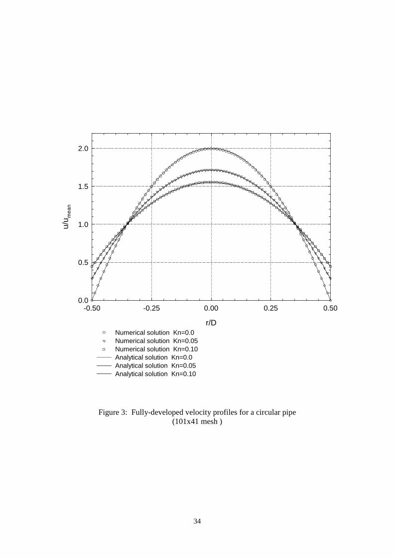
The validation tests compared the analytical velocity profiles given in eqns. (41)& (43) against predictions from the downstream boundary of the numerical model.Three separate Knudsen numbers ( 0 , 0.05 and 0.10Kn = ) were considered and theReynolds number for the numerical simulations was set to its highest value( 400Re = ). Choosing to run the tests at the highest Reynolds number (longesthydrodynamic development length) allowed an immediate assessment of thesuitability of the hydrodynamic mesh. If a chosen mesh had insufficient length toallow full development of the velocity profile, the numerical predictions would haveshown obvious discrepancies against the analytical solution.

The results for the circular pipe and parallel plate geometry are presented innon-dimensionalised form in Figures 3 & 4. Both sets of velocity profiles showexcellent agreement between the numerical and analytical solutions, clearly validatingthe hydrodynamic model. Slight discrepancies can be seen at the centreline of the

12

circular pipe for a Knudsen number, 0Kn = , but the maximum error amounts to lessthan 0.15%.

Figures 3 & 4 also provide a useful visualisation of the changes which takeplace in the velocity profile as non-continuum flow effects start to dominate. It can beseen that as the Knudsen number increases, the maximum velocity at the centre of theduct decreases whilst the tangential slip-velocity at the wall increases. The net effectof these changes is to produce a velocity profile which becomes more uniform withincreasing Knudsen number. Another interesting feature of the flow redistribution isthe fact that the velocity remains invariant with respect to Knudsen number at twolocations across the duct. It can readily be shown that for the circular pipe, theposition of this feature occurs at

1

2 2

r

D= ± (45)

whilst for flow between parallel plates, the feature occurs at

1 1

2 2 3

y

H= ± (46)

6.2 Hydrodynamic development lengths

After validating the hydrodynamic code against the analytical fully-developedvelocity profiles, the numerical model was then used to examine the effects of theReynolds number and the Knudsen number on the entrance development length. Aspreviously described in Section 4, the computations for the entrance length werebased upon the 99% velocity cut-off point.

6.2.1 Circular pipe

Tables 1 & 2 present non-dimensionalised hydrodynamic development lengths (L/D)for three separate Knudsen numbers ( 0 , 0.05 and 0.10Kn = ) and a range ofReynolds numbers between 1 and 400. The results in Table 1 were evaluated using a101q41 hydrodynamic mesh whilst the results in Table 2 employed a much higherresolution 201q101 mesh. The computed hydrodynamic development lengths for thetwo grid resolutions were found to be very similar and consequently meshindependent results were judged to be achieved using the 101q41 mesh.

Figure 5 illustrates the entrance development length as a function of Reynoldsnumber for the 101q41 mesh. Superimposed on the present results are the continuumdevelopment length equations presented by Atkinson et al. [12] and Chen [14].Atkinson et al. suggested that the non-dimensionalised development length can berelated to the Reynolds number via a simple linear relationship:

13

0.59 0.056L

ReD

= + (47)

whilst Chen [14] analysed development length data originally presented by Friedmannet al. [11] and proposed a more elaborate function of the form:

0.600.056

0.035 1

LRe

D Re= +

+(48)

Figures 5 demonstrates that the present numerical results are in excellent agreementwith the entrance lengths predicted by eqn. (48). In addition, it can be seen thatAtkinson et al.’s solution tends to over-predict the development length at all but thelowest Reynolds numbers. This is confirmed in Figure 6 which shows an enlargedview of the development length variations for 0 100Re≤ ≤ . Figure 6 also illustratesthat the entrance length for a circular pipe tends towards an L/D ratio ofapproximately 0.60 as the Reynolds number approaches zero. Consequently, at lowReynolds numbers, the fully-developed velocity profile is established within about 0.6pipe diameters of the entrance.

Figures 7 & 8 repeat the development length plots for the high resolution201q101 mesh (Table 2). Comparison of the graphs for the two grid resolutionsimmediately confirms that mesh independent results are achieved using the lowerresolution 101q41 grid. The results also demonstrate that rarefaction effects onlyhave a marginal effect on the development length in circular pipes. It can therefore beconcluded that Chen’s development length formula (eqn. 48) derived for continuumflows is equally valid in the slip-flow regime.

6.2.2 Flow between parallel plates

Table 3 presents the corresponding hydrodynamic development lengths for theparallel plate geometry. A mesh resolution study was undertaken, and it was foundthat the 101q41 hydrodynamic grid once again yielded mesh independent results. Itshould be noted both the non-dimensionalised development length and the Reynoldsnumber are based upon the hydraulic diameter of the duct, hD .

The entrance lengths are illustrated in Figures 9 & 10 together with thedevelopment length equations presented by Atkinson et al. [12] and Chen [14]. In thecase of flow between parallel plates, Atkinson et al. suggested that the non-dimensionalised development length can be related to the Reynolds number via thefollowing linear relationship:

0.3125 0.011h

LRe

D= + (49)

whereas Chen [14] suggested a more elaborate function of the form:

14

0.3150.011

0.0175 1h

LRe

D Re= +

+(50)

Figures 9 & 10 indicate that the present continuum results ( 0Kn = ) are in goodagreement with the hydrodynamic entrance lengths predicted by eqn. (50). It can alsobe seen that Atkinson et al.’s solution again tends to over-predict the developmentlengths except at very low Reynolds numbers. More importantly, the present resultsshow that the Knudsen number has a significant effect on the length of thedevelopment region. Inspection of the L/Dh values in Table 3 reveals that at aReynolds number of 400, the entrance length for a Knudsen number of 0.1 is 26%longer than the corresponding no-slip solution. Even at relatively low Reynoldsnumbers, the increase in hydrodynamic development length may still be important.For example, at a Reynolds number of 10, the entrance length for a Knudsen numberof 0.1 is 13.6% longer than the continuum solution. It can therefore be concluded thatthe development length formulae proposed by Atkinson et al. [12] and Chen [14] forthe parallel plate geometry cannot be applied to the slip-flow regime and consequentlya new development length equation accounting for the variation in both the Reynoldsnumber and Knudsen number must be evaluated.

To provide extra data for the subsequent least-squares analysis, additionaldevelopment lengths were computed for Knudsen numbers of 0.025 and 0.075(midway between the existing Knudsen numbers). Table 4 presents the complete setof entrance lengths employed in the analysis whilst Figure 11 provides a 3-dimensional representation of the data. A non-linear least-squares surface-fittingprocedure employing the Levenberg-Marquardt method [38] was used to determinethe equation of best fit; the analysis being performed using SigmaPlot, a commercialcurve-fitting and graph plotting package. The effect of the Knudsen number wastaken into account by multiplying Chen’s original development length equation bycorrection factors of the form:

1

1

A Kn

B Kn

′ + ′+

(51)

where A and B are constants and Kn′ is defined as

2Kn Kn

− σ′ =σ

(52)

The Knudsen number variation shown in (51) was chosen because the analytical slip-flow equations developed in Appendix B have similar modification factors. Applyingthe Levenberg-Marquardt least-squares technique yields the following expression forthe hydrodynamic development length:

0.320 1 13.51 1 14.750.011

0.0272 1 1 12.11 1 9.77h

L Kn KnRe

D Re Kn Kn

′ ′ + += + ′ ′+ + + (53)

15

Estimation of the likely errors in each of the coefficients reveals that it is probablybetter to ignore the Knudsen number correction in the first term of eqn. (53) since thecoefficients of 13.51 and 12.11 cannot be determined with any degree of accuracy.Consequently, a second least-squares analysis was conducted using a Knudsennumber dependency on just the last term, giving:

0.332 1 14.780.011

0.0271 1 1 9.78h

L KnRe

D Re Kn

′ += + ′+ + (54)

Figure 12 illustrates the surface fit presented in eqn. (54). It can be seen that theproposed equation provides a good fit to the development length data over the rangeof Reynolds numbers considered. Moreover, the linearity of the Reynolds numberdependency in the second term of eqn. (54) implies that the expression should providea reliable estimate of hydrodynamic development lengths up to the transition toturbulence at approximately Re=2000. The proposed entrance length equation istherefore appropriate for the entire laminar slip-flow regime.

7 Conclusions

An investigation of low Reynolds number rarefied gas flows in circular pipes andparallel plates has been conducted using a specially adapted two-dimensional finite-volume Navier-Stokes solver. The hydrodynamic model is applicable to the slip-flowregime which is valid for Knudsen numbers between 0 0.1Kn< ≤ . Within this range,rarefaction effects are important but the flow can still be modelled using the Navier-Stokes equations provided appropriate tangential slip-velocity boundary conditionsare implemented along the walls of the flow domain.

The present study examines the effects of the Reynolds number and theKnudsen number on the hydrodynamic development length in circular pipes andparallel plates. Model validation has been accomplished by comparing numerical andanalytical fully-developed velocity profiles across the ducts. In addition,hydrodynamic entrance lengths for the continuum (no-slip) regime are compared withdata published in earlier studies. The results from the hydrodynamic model show thatdevelopment lengths for the circular pipe are only marginally affected by rarefaction.However, it has been found that the Knudsen number can have a significant effect onthe entrance development region for flows between parallel plates. At the upper limitof the slip-flow regime ( 0.1Kn ; ), entrance lengths for the parallel plate geometrycan be up to 25% longer than the corresponding continuum solution. It is thereforeimportant for designers of microfluidic devices to account for the possibility ofincreased development lengths in the gaseous slip-flow regime.

16

References

[1] Schlichting, H. Boundary-Layer Theory, 3rd English Ed., McGraw-Hill, 1968.[2] Schlichting, H. Laminare Kanaleinlaufstromung, Z.A.M.M., Vol. 14, pp. 368-

373, 1934.[3] Goldstein, S. Modern Developments in Fluid Dynamics, Vol. 1, Clarendon

Press, Oxford, 1938: Atkinson & Goldstein, p. 304.[4] Davies, R.T. Laminar incompressible flow past a semi-infinite flat plate, J.

Fluid Mech., Vol. 27, pp. 691-704, 1967.[5] Van Dyke, M. Entry flow in a channel, J. Fluid Mech., Vol. 44, pp. 813-823,

1970.[6] Langhaar, H.L. Steady flow in the transition length of a straight tube, Trans. of

the ASME, J. Applied Mech., Vol. 9, A55-A58, 1942.[7] Lundgren, T.S., Sparrow, E.M. & Starr, J.B. Pressure drop due to the entrance

region in ducts of arbitrary cross-section, Trans. of the ASME, J. BasicEngineering, pp. 620-626, 1964.

[8] Han, L.S. Hydrodynamic entrance lengths for incompressible laminar flow inrectangular ducts, Trans. of the ASME, J. Applied Mechanics, Vol. 27, pp. 403-409, 1960.

[9] Bodoia, J.R. & Osterle, J.F. Finite-difference analysis of plane Poiseuille andCouette flow developments, Applied Scientific Research, Section A, Vol. 10,pp. 265-276, 1961.

[10] Wang, Y.L. & Longwell, P.A. Laminar flow in the inlet section of parallelplates, A.I.Ch.E. Journal, Vol. 10, No. 3, pp. 323-329, 1964.

[11] Friedmann, M., Gillis, J. & Liron, N. Laminar flow in a pipe at low andmoderate Reynolds numbers, Applied Scientific Research, Vol. 19, pp. 426-438,1968.

[12] Atkinson, B., Brocklebank, M.P., Card, C.C.H. & Smith, J.M. Low Reynoldsnumber developing flows, A.I.Ch.E. Journal, Vol. 15, No. 4, pp. 548-553, 1969.

[13] Morihara, H. & Cheng, R.T.S. Numerical solution of the viscous flow in theentrance region of parallel plates, J. Computational Physics, Vol. 11, pp. 550-572, 1973.

[14] Chen, R.Y. Flow in the entrance region at low Reynolds numbers, Trans. of theASME, J. Fluids Engineering, Vol. 95, pp. 153-158, 1973.

[15] Sparrow, E.M., Lundgren, T.S. & Lin, S.H. Slip flow in the entrance region ofa parallel plate channel, Proc. Heat Transfer and Fluid Mechanics Inst.,Stanford University Press, Paper no. 16, pp. 223-238, 1962.

[16] Ebert, W.A. & Sparrow, E.M. Slip flow in rectangular and annular ducts,Trans. of the ASME, J. Basic Engineering, Vol. 87, pp. 1018-1024, 1965.

[17] Sreekanth, A.K. Slip flow through long circular tubes, Rarefied Gas Dynamics6, pp. 667-680, Academic Press, New York, 1968.

[18] Quarmby, A. A finite-difference analysis of developing slip flow, AppliedScientific Research, Vol. 19, pp. 18-33, 1968.

17

[19] Gampert, B. Inlet flow with slip, Rarefied Gas Dynamics 10, pp. 225-235,1976.

[20] Gabriel, K., Jarvis, J. & Trimmer, W. (eds.) Small Machines, LargeOpportunities: a report on the emerging field of microdynamics, NationalScience Foundation, AT&T Bell Laboratories, Murray Hill, New Jersey, USA,1988.

[21] Gravesen, P., Branebjerg, J. & Jenson, O.S. Microfluidics – a review, J.Micromechanics and Microengineering, Vol. 3, pp. 168-182, 1993.

[22] Gad-el-Hak, M. The fluid mechanics of microdevices – The Freeman ScholarLecture, J. of Fluids Engineering, Vol. 121, pp. 5-33, 1999.

[23] Beskok, A. & Karniadakis, G.E. Simulation of heat and momentum transfer incomplex microgeometries, J. Thermophysics and Heat Transfer, Vol. 8, No. 4,1994.

[24] Beskok, A., Karniadakis, G.E. & Trimmer, W. Rarefaction, compressibility andthermal creep effects in micro-flows, Proc. of the ASME Dynamic Systems andControl Division, pp. 877-892, ASME, 1995.

[25] Pfahler, J., Harley, J., Bau, H. & Zemel, J.N. Gas and liquid flow in smallchannels, DSC-Vol. 32, Micromechanical Sensors, Actuators and Systems, pp.49-60, ASME, 1991.

[26] Harley, J.C., Huang, Y., Bau, H.H. & Zemel, J.N. Gas flow in microchannels,J. Fluid Mech., Vol. 284, pp. 257-274, 1995.

[27] Arkilic, E.B. & Breuer, K.S. Gaseous flow in small channels, AIAA Shear FlowConference, Paper no. AIAA 93-3270, Orlando, 1993.

[28] Arkilic, E.B., Breuer, K.S. & Schmidt, M.A. Gaseous flow in microchannels,FED-Vol. 197, Application of Microfabrication to Fluid Mechanics, pp. 57-66,ASME, 1994.

[29] Arkilic, E.B., Schmidt, M.A. & Breuer, K.S. Gaseous slip flow in longmicrochannels, J. of Micro-Electro-Mechanical Systems, Vol. 6, No. 2, pp. 167-178, 1997.

[30] Arkilic, E.B. Measurement of the mass flow and tangential momentumaccommodation coefficient in silicon micromachined channels, Ph.D. Thesis,Massachusetts Institute of Technology, Cambridge, Massachusetts, 1997.

[31] Basset, A.B. A Treatise on Hydrodynamics, Cambridge University Press, 1888.[32] Schaaf, S.A. & Chambre, P.L. Flow of Rarefied Gases, Princeton University

Press, 1961.[33] Thomas, L.B. & Lord, R.G. Comparative measurements of tangential

momentum and thermal accommodations on polished and on roughened steelspheres, Rarefied Gas Dynamics 8, pp. 405-412, ed. K. Karamcheti, AcademicPress, New York, 1974.

[34] Arkilic, E.B., Schmidt, M.A. & Breuer, K.S. TMAC measurement in siliconmicromachined channels, Rarefied Gas Dynamics 20, Beijing University Press,1997.

[35] Shah, R.K. & London, A.L. Laminar Flow Forced Convection in Ducts,Academic Press, New York, 1978.

18

[36] White, F.M. Viscous Fluid Flow, 2nd Edition, McGraw-Hill, 1991.[37] Gu X.J. & Emerson, D.R. THOR-2D: A two-dimensional computational fluid

dynamics code, Technical Report, Department of Computational Science andEngineering, CLRC Daresbury Laboratory, June 2000.

[38] Press, W.H., Teukolsky, S.A., Vetterling, W.T. & Flannery, B.P. NumericalRecipes in Fortran: The Art of Scientific Computing, 2nd Ed., CambridgeUniversity Press, 1994.

[39] CRC Handbook of Chemistry and Physics, 80th Ed., CRC Press, 1999-2000.

19

Appendix A

Analysis of fully-developed laminar slip flow within a circular pipe

Consider an incompressible Newtonian fluid of density, ρ and viscosity, µ flowingthrough a long straight tube having a circular cross-section of radius, R. Let x denotethe longitudinal distance along the axis of the pipe and let r denote the radial co-ordinate measured outwards from the centreline. Under fully-developed flowconditions, the velocity components in the radial- and tangential-directions are zerowhilst the velocity component parallel to the longitudinal axis (denoted by u) is solelydependent upon r. In addition, the pressure is constant over a given cross-section ofthe pipe. Therefore, under fully-developed conditions, the flow can be describedcompletely by the axial-direction Navier-Stokes equation, which in cylindrical co-ordinates reduces to

2

2

1d u du dp

dr r dr dx

µ + =

(1)

where /dp dx is the pressure gradient in the longitudinal direction.In order to account for non-continuum flow effects, eqn. (1) is solved in

conjunction with the slip-velocity boundary condition proposed by Basset [31]:

t tuτ = β (2)


2µβ =

− σ λ σ

(3)

where N is the coefficient of viscosity, σ is the tangential momentum accommodationcoefficient (TMAC) and λ is the mean free path of the gas. The tangential momentumaccommodation coefficient is introduced into the equation to account for thereduction in the momentum of the molecules colliding with the wall. The value of theTMAC depends upon the particular solid and gas involved and also on the surfaceroughness of the wall. Equations (2) and (3) can be combined and rearranged to give

2t tu

− σ λ= τσ µ

(4)

At this stage, it is convenient to recast the mean free path in eqn. (4) in terms ofa non-dimensionalised Knudsen number, Kn. For compatibility with the standarddefinition of Reynolds number for circular pipes, the characteristic length scale in the

20

present analysis is defined as the pipe diameter, D. Thus, eqn. (4) can be rewritten as

2t t

Kn Du

− σ= τσ µ

(5)

where Kn is defined as the ratio of the mean free path of the molecules (λ) to thediameter of the pipe:

KnD

λ= (6)

The shear stress on the pipe wall ( r R= ) can be related to the velocity gradient asfollows:

tr R

du

dr =

τ = −µ (7)

The negative sign is introduced into the above expression to account for the fact thatthe velocity gradient, du/dr is negative. Substituting eqn. (7) into (5) then yields thetangential slip-velocity as

2t

r R

duu Kn D

dr =

− σ= −σ

(8)

The axial-direction Navier-Stokes equation (1) is a linear, second-order ordinarydifferential equation. It is assumed that the solution of (1) yields a velocity profile ofthe form:

2( )u r a r b r c= + + (9)

where a, b and c are constants. Repeated differentiation of eqn. (9) gives

( ) 2

( ) 2

u r a r b

u r a

′ = +

′′ = (10)

and substituting the derivatives shown in (10) into the original differential equationyields

( )1 12 2

dpa a r b

r dx+ + =

µ(11)

which can be rearranged to give

21

14 0

dpa r b

dx

− + = µ (12)

Inspection of eqn. (12) thus reveals

1and 0

4

dpa b

dx= =

µ(13)

The zero-order coefficient, c, is determined using the slip-velocity constraint shown ineqn. (8). First, the velocity gradient at the wall is found by substituting 0b = intoeqn. (10):

2r R

du R dp

dr dx=

=µ

(14)

Hence, the tangential slip-velocity at the wall is given by

2

2t

R dpu Kn D

dx

− σ= −σ µ

(15)

or22 1

t

dpu Kn R

dx

− σ= −σ µ

(16)

The tangential slip-velocity is then substituted into the velocity profile proposed ineqn. (9):

2 21 2 1

4

dp dpR c Kn R

dx dx

− σ+ = −µ σ µ

(17)

which can be rearranged to give

2 21 24

4

dpc R Kn R

dx

− σ = − + µ σ (18)

Thus the velocity profile across the pipe is given by

2 2 21 1 2( ) 4

4 4

dp dpu r r R Kn R

dx dx

− σ = − + µ µ σ (19)

which can be rewritten as

2 2 21 2( ) 4

4

dpu r R r Kn R

dx

− σ = − − + µ σ (20)

It can therefore be seen that the velocity profile over the cross-section takes the formof a paraboloid of revolution. As an aside, in the limit of 0Kn → (continuum flow)

22

we obtain the no-slip (NS) solution given by Hagen-Poiseuille theory for flow througha circular pipe (see Schlichting [1] ):

( )2 2NS

1( )

4

dpu r R r

dx= − −

µ(21)

The maximum velocity in the pipe occurs at the centreline ( 0r = ):

2

max

21 4

4

R dpu Kn

dx

− σ = − + µ σ (22)

In addition, let u denote the mean or average velocity in the pipe, defined by

2

0

1( ) 2

R

u u r r drR

= ππ

⌠⌡

(23)

Substituting eqn. (20) into (23) yields

2 2 22

0

1 1 24 2

4

R

dpu R r Kn R r dr

R dx

− σ = − − + π π µ σ

⌠⌡

(24)

which can be simplified to

2 3 22

0

1 2 24

4

R

dpu R r r Kn R r dr

dx R

− σ = − − + µ σ

⌠⌡

(25)

Integrating and rearranging finally leads to the mean velocity:

2 1 21 8

4 2

R dpu Kn

dx

− σ = − + µ σ (26)

Hence, the ratio of the maximum velocity at the centreline of the pipe to the meanvelocity is given by

max

21 4

1 21 8

2

Knu

uKn

− σ + σ =− σ + σ

(27)

and therefore the maximum velocity in the pipe is found to be

23

max

21 4

22

1 8

Kn

u u

Kn

− σ + σ =− σ + σ

(28)

Allowing 0Kn → yields the familiar no-slip (NS) solution given by Hagen-Poiseuillepipe theory:

max(NS) 2u u= (29)

Similarly, eqns. (20) and (26) can be combined to give the velocity distribution acrossthe pipe in terms of the mean velocity:

2

2

21 4

( )

1 21 8

2

rKn

u r R

uKn

− σ− + σ =− σ + σ

(30)

or2

2

21 4

( ) 22

1 8

rKn

Ru r u

Kn

− σ− + σ =− σ + σ

(31)

The tangential slip-velocity at the wall, tu , can then be found by prescribing r R= ineqn. (31):

28

21 8

t

Knu u

Kn

− σσ=

− σ + σ

(32)

In addition, the volume rate of flow in the circular pipe is given by

42 2

1 88

R dpQ R u Kn

dx

π − σ = π = − + µ σ (33)

Hence, in the limit of 0Kn → we obtain the no-slip (NS) solution for the volume rateof flow:

42

NS NS 8

R dpQ R u

dx

π= π = −µ

(34)

24

Dividing eqn. (33) by (34) yields

NS

21 8

QKn

Q

− σ= +σ

(35)

The above equation indicates that even at relatively low Knudsen numbers, the slip-velocity boundary condition substantially increases the volume rate of flow throughthe pipe.

Finally, substituting eqn. (32) for the tangential slip-velocity at the wall intoeqn. (2) yields the shear stress on the wall:

28

2 21 8

t

Knu

Kn

− σµ στ =− σ − σ λ + σ σ

(36)


8

21 8

t

u

D Kn

µτ =− σ + σ

(37)

Furthermore, by defining the Reynolds number, Re, in the pipe as

u DRe

ρ=µ

(38)

eqn. (37) can be expressed as

2

2

8

21 8

t

Re

D Kn

µτ =

− σ ρ + σ

(39)

The no-slip solution is found by considering 0Kn → . This yields the shear stress onthe wall as

2

(NS) 2

8t

Re

D

µτ =

ρ(40)

25

Appendix B

Analysis of fully-developed laminar slip flow between parallel plates

The analysis of laminar slip flow between parallel plates essentially follows a similarprocedure to that detailed in Appendix A for circular pipes. The geometry isimportant as it forms the limiting flow condition for large aspect ratio rectangularducts commonly encountered in microfluidic devices.

Consider an incompressible Newtonian fluid of density, ρ and viscosity, µflowing between two parallel plates separated by a distance, H, as illustrated in thediagram below:

Figure B1: Slip flow between parallel plates

Let x denote the longitudinal distance along the duct and let y denote the normaldistance measured upwards from the lower wall. Under fully-developed flowconditions, the velocity component in the y-direction vanishes and the velocitycomponent in the x-direction (denoted by u) is solely dependent upon y. In addition,the pressure is constant over a given cross-section of the duct. Therefore, under fully-developed conditions, the flow can be described completely by the x-direction Navier-Stokes equation which reduces to

2

2

d u dp

dy dxµ = (1)

where /dp dx is the pressure gradient in the longitudinal direction.In order to account for non-continuum flow effects, eqn. (1) is solved in

conjunction with the slip-velocity boundary condition proposed by Basset [31]:

t tuτ = β (2)


Lower wall ( 0y = )

Upper wall ( y H= )

Centreline ( / 2y H= )

x

yH

26

2µβ =

− σ λ σ

(3)

where N is the coefficient of viscosity, σ is the tangential momentum accommodationcoefficient (TMAC) and λ is the mean free path of the molecules. Equations (2) and(3) can be combined and rearranged to give

2t tu

− σ λ= τσ µ

(4)

At this stage, it is convenient to recast the mean free path in eqn. (4) in terms ofthe non-dimensionalised Knudsen number, Kn. Analyses of non-circular ductsgenerally rely upon the concept of the hydraulic diameter, hD , as detailed bySchlichting [1], Shah & London [35] or White [36]:

4 area 4

wetted perimeterh

AD

P

×= = (5)

Thus it is customary to define the Reynolds number in non-circular ducts in terms ofthe hydraulic diameter, i.e.

hu DRe

ρ=µ

(6)

where u is the mean or average velocity in the duct. In the case of flow betweenparallel plates, it can readily be shown that the hydraulic diameter is twice theseparation of the plates:

2hD H= (7)

and therefore the Reynolds number in the present analysis is defined as

2u HRe

ρ=µ

(8)

For compatibility with the above definition of Reynolds number, the hydraulicdiameter should also be employed as the characteristic length scale when determiningthe Knudsen number, Kn. Consequently, the tangential slip-velocity equation (4) canbe rewritten as

2 2t t

Kn Hu

− σ= τσ µ

(9)

where Kn is defined as the ratio of the mean free path of the molecules (λ) to the

27

hydraulic diameter:

2h

KnD H

λ λ= = (10)

The shear stress on the lower wall of the duct ( 0y = ) can be related to thevelocity gradient as follows:

0

t

y

du

dy =

τ = µ (11)

As an aside, the shear stress on the upper wall of the duct ( y H= ) is evaluated usinga very similar equation with the exception of a negative sign to account for the changein direction of the velocity gradient at the upper wall. Substituting eqn. (11) into (9)then yields the tangential slip-velocity as

0

22t

y

duu Kn H

dy =

− σ=σ

(12)

The x-direction Navier-Stokes equation (1) is a linear, second-order ordinarydifferential equation. It is assumed that the solution of (1) yields a velocity profile ofthe form:

2( )u y a y b y c= + + (13)

where a, b and c are constants. Repeated differentiation of eqn. (13) yields

( ) 2

( ) 2

u y a y b

u y a

′ = +

′′ = (14)

and substituting the second derivative, ( )u y′′ into the original differential equationgives

1

2

dpa

dx=

µ(15)

The first-order coefficient, b, is determined by employing the fact that the velocityprofile between the plates is symmetrical. Consequently,

( ) 0 at2

Hu y y′ = = (16)

giving

2

H dpb a H

dx= − = −

µ(17)

28

Finally, the zero-order coefficient, c, is evaluated using the slip-velocity constraintshown in eqn. (12). The velocity gradient at the lower wall is found by substituting

0y = into eqn. (14) giving

02

y

du H dp

dy dx=

= −µ

(18)

and therefore the tangential slip-velocity is given by

22

2t

H dpu Kn H

dx

− σ= −σ µ

(19)

The tangential slip-velocity is then substituted back into the velocity profile shown ineqn. (13) to give

22 1 dpc Kn H

dx

− σ= −σ µ

(20)

Thus the velocity profile across the duct takes the form:

2 21 2 1( )

2 2

dp H dp dpu y y y Kn H

dx dx dx

− σ= − −µ µ σ µ

(21)


2 2

2

2( ) 2

2

H dp y yu y Kn

dx H H

− σ= − − + µ σ (22)

As an aside, in the limit of 0Kn → (continuum flow) we obtain the familiar no-slip(NS) formula for parallel flow through a straight channel (see Schlichting [1] ):

2 2

NS 2( )

2

H dp y yu y

dx H H

= − − µ

(23)

The maximum velocity occurs at the centreline of the duct ( / 2y H= ):

2

max

1 1 22

2 2 4

H dpu Kn

dx

− σ = − − + µ σ (24)

or

2

max

1 21 8

2 4

H dpu Kn

dx

− σ = − + µ σ (25)

29

In addition, let u denote the mean or average velocity in the duct, defined by

0

1( )

H

u u y dyH

= ⌠⌡

(26)

Substituting eqn. (22) into (26) yields

2 2

2

0

1 22

2

H

H dp y yu Kn dy

H dx H H

− σ= − − + µ σ

⌠⌡

(27)

Integrating and rearranging leads to the mean velocity:

2 1 21 12

2 6

H dpu Kn

dx

− σ = − + µ σ (28)

Hence, the ratio of the maximum velocity to the mean velocity is given by

max

21 1 84

1 21 126

Knu

uKn

− σ + σ =− σ + σ

(29)

and therefore the maximum velocity in the duct equals

max

21 8

3

2 21 12

Knu u

Kn

− σ + σ =− σ + σ

(30)

Allowing 0Kn → yields the familiar no-slip solution:

max(NS)3

2u u= (31)

Similarly, eqns. (22) and (28) can be combined to give the velocity distribution acrossthe duct in terms of the mean velocity:

30

2

2

22

( )

1 21 12

6

y yKn

H Hu y

uKn

− σ− + σ =− σ + σ

(32)

or2

2

22

( ) 62

1 12

y yKn

H Hu y u

Kn

− σ− + σ =− σ + σ

(33)

The tangential slip-velocity at the wall, tu , can then be found by prescribing 0y = ineqn. (33):

212

21 12

t

Knu u

Kn

− σσ=

− σ + σ

(34)

In addition, the volume rate of flow per unit width of duct, q, is given by

3 1 21 12

2 6

H dpq H u Kn

dx

− σ = = − + µ σ (35)

Hence, in the limit of 0Kn → we obtain the no-slip solution for the volume rate offlow:

3

NS NS

1

2 6

H dpq H u

dx= = −

µ(36)

Dividing eqn. (35) by (36) yields

NS

21 12

qKn

q

− σ= +σ

(37)

The above equation indicates that even at relatively low Knudsen numbers, the slip-velocity boundary condition substantially increases the volume rate of flow throughthe duct.

Finally, substituting eqn. (34) for the tangential slip-velocity at the wall intoeqn. (2) yields the shear stress on the wall:

31

212

2 2121

t

Knu

Kn

− σµ στ =− σ − σ λ + σ σ

(38)


12

22 121

t

u

H Kn

µτ =− σ + σ

(39)

Furthermore, since the Reynolds number in the duct is defined as

2u HRe

ρ=µ

(40)

eqn. (39) can be expressed as

2

2

3

2121

t

Re

H Kn

µτ =

− σ ρ + σ

(41)

The no-slip solution is found by considering 0Kn → . This yields the shear stress onthe wall as

2

(NS) 2

3t

Re

H

µτ =

ρ(42)

32

Appendix C

Determination of the mean free path of a gas

For an ideal gas modelled as rigid spheres of diameter, σ , the mean distance travelledby a molecule between successive collisions or mean free path, λ, is given by [39]:

22

k T

pλ =

π σ(1)

where,23

2

Boltzmann’s constant 1.380662 10 J / K,

temperature (K),

pressure (N/m ) and

collision diameter of the molecules (m).

k

T

p

−= = ×==

σ =

At standard ambient temperature and pressure (SATP), defined as T 298.15 K= and5 210 N/mp = , eqn. (1) becomes:

27

2

9.265 10−×λ =σ

(2)

For air, the average collision diameter of the molecules is 103.66 10−× m giving a meanfree path of 86.92 10−× m (or 69.2 nm).

The table below details the collision diameters of other common gases.

Gas σ (m)

Air 3.66q10-10

Ar 3.58q10-10

CO2 4.53q10-10

H2 2.71q10-10

He 2.15q10-10

Kr 4.08q10-10

N2 3.70q10-10

NH3 4.32q10-10

Ne 2.54q10-10

O2 3.55q10-10

Xe 4.78q10-10

Table C1: Collision diameters of common gases [39]

33

Figure 1: Schematic layout of boundary conditions for circular pipe geometry

Figure 2: Schematic layout of boundary conditions for parallel plate geometry

Flow direction1

0

u

v

==0x = x l=

Inflow0

0

u

xv

x

∂ =∂∂ =∂

Outflow

0 0u

vr

∂ = =∂

Centreline 0r =

Wall r R=

20

r R

uu Kn D v

r =

− σ ∂= − =σ ∂

Flow direction1

0

u

v

==0x = x l=

Inflow0

0

u

xv

x

∂ =∂∂ =∂

Outflow

0 0u

vy

∂ = =∂

Centreline / 2y H=

Wall y H=

22 0

y H

uu Kn H v

y =

− σ ∂= − =σ ∂

34

Figure 3: Fully-developed velocity profiles for a circular pipe(101x41 mesh )

r/D

-0.50 -0.25 0.00 0.25 0.50

u/u m

ean

0.0

0.5

1.0

1.5

2.0

Numerical solution Kn=0.0Numerical solution Kn=0.05 Numerical solution Kn=0.10Analytical solution Kn=0.0Analytical solution Kn=0.05Analytical solution Kn=0.10

35

Figure 4: Fully-developed velocity profiles for flow between parallel plates(101x41 mesh )

y/H

0.00 0.25 0.50 0.75 1.00

u/u m

ean

0.0

0.5

1.0

1.5

Numerical solution Kn=0.0Numerical solution Kn=0.05 Numerical solution Kn=0.10Analytical solution Kn=0.0Analytical solution Kn=0.05Analytical solution Kn=0.10

36

Kn=0.0 Kn=0.05 Kn=0.10Re

L/D L/D L/D1 0.6238 0.6618 0.67535 0.7126 0.7564 0.7746

10 0.8799 0.9254 0.945420 1.3483 1.3835 1.395340 2.4331 2.4480 2.446360 3.5483 3.5500 3.539480 4.6780 4.6670 4.6470100 5.8035 5.7816 5.7564150 8.6236 8.5707 8.5330200 11.4460 11.3652 11.3158250 14.2749 14.1606 14.0974300 17.0736 16.9215 16.8450350 19.7880 19.6097 19.5247400 22.3624 22.1373 22.0322

Table 1: Non-dimensionalised development lengths for a circular pipe(101 � 41 mesh)

Kn=0.0 Kn=0.05 Kn=0.10Re

L/D L/D L/D1 0.6210 0.6579 0.67325 0.7094 0.7528 0.771810 0.8766 0.9221 0.941820 1.3462 1.3791 1.392440 2.4303 2.4444 2.442860 3.5462 3.5473 3.536280 4.6689 4.6590 4.6400

100 5.7931 5.7732 5.7472150 8.6017 8.5612 8.5222200 11.4061 11.3497 11.2999250 14.2025 14.1337 14.0728300 16.9717 16.8925 16.8229350 19.6703 19.5786 19.4996400 22.2270 22.1284 22.0392

Table 2: Non-dimensionalised development lengths for a circular pipe(201 � 101 mesh)

37

Figure 5: Non-dimensionalised development lengths for a circular pipe(101 � 41 mesh)

Re

0 100 200 300 400

L/D

0

5

10

15

20

25

Kn=0.0Kn=0.05Kn=0.10Atkinson et al. (Kn=0.0)Chen (Kn=0.0)

38

Figure 6: Detail of non-dimensionalised development lengths for acircular pipe (101 � 41 mesh)

Re

0 20 40 60 80 100

L/D

0

2

4

6

8


39

Figure 7: Non-dimensionalised development lengths for a circular pipe(201 � 101 mesh)

Re

0 100 200 300 400

L/D

0

5

10

15

20

25


40

Figure 8: Detail of non-dimensionalised development lengths for acircular pipe (201 � 101 mesh)

Re

0 20 40 60 80 100

L/D

0

2

4

6

8


41

Kn=0.0 Kn=0.05 Kn=0.10Re

L/Dh L/Dh L/Dh

1 0.3238 0.3473 0.34885 0.3360 0.3646 0.370310 0.3544 0.3915 0.402720 0.4092 0.4636 0.484940 0.5706 0.6583 0.697560 0.7769 0.8892 0.943680 0.9945 1.1316 1.2016

100 1.2141 1.3795 1.4640150 1.7589 2.0057 2.1296200 2.2966 2.6340 2.7994250 2.8240 3.2633 3.4711300 3.3425 3.8916 4.1447350 3.8533 4.5224 4.8151400 4.3555 5.1509 5.4898

Table 3: Non-dimensionalised development lengths for flow between parallel plates(101 � 41 mesh)

42

Figure 9: Non-dimensionalised development lengths for flow between parallel plates(101 � 41 mesh)

Re

0 100 200 300 400

L/D

h

0

1

2

3

4

5

6


43

Figure 10: Detail of non-dimensionalised development lengths for flow betweenparallel plates (101 � 41 mesh)

Re

0 20 40 60 80 100

L/D

h

0.0

0.5

1.0

1.5


44

Kn=0.0 Kn=0.025 Kn=0.05 Kn=0.075 Kn=0.10Re

L/Dh L/Dh L/Dh L/Dh L/Dh

1 0.3238 0.3389 0.3473 0.3495 0.34885 0.3360 0.3532 0.3646 0.3696 0.370310 0.3544 0.3776 0.3915 0.3999 0.402720 0.4092 0.4407 0.4636 0.4783 0.484940 0.5706 0.6168 0.6583 0.6841 0.697560 0.7769 0.8337 0.8892 0.9241 0.943680 0.9945 1.0619 1.1316 1.1762 1.2016

100 1.2141 1.2954 1.3795 1.4338 1.4640150 1.7589 1.8808 2.0057 2.0846 2.1296200 2.2966 2.4674 2.6340 2.7392 2.7994250 2.8240 3.0528 3.2633 3.3951 3.4711300 3.3425 3.6393 3.8916 4.0505 4.1447350 3.8533 4.2235 4.5224 4.7083 4.8151400 4.3555 4.8059 5.1509 5.3642 5.4898

Table 4: Non-dimensionalised development lengths for flow between parallel plates(101 � 41 mesh)

45

Figure 11: 3-dimensional representation of non-dimensionalised development lengthsfor flow between parallel plates

0

1

2

3

4

5

6

0

100

200

300

400

0.000

0.025

0.050

0.075

0.100

L/D

h

Reynolds number

Knudsen number

46

Figure 12: Least-squares surface fit of non-dimensionalised development lengths for flow between parallel plates

Re

0 100 200 300 400

L/D

h

0

1

2

3

4

5

6

Kn=0.0Kn=0.05Kn=0.10Least-squares fit Kn=0.0Least-squares fit Kn=0.05Least-squares fit Kn=0.10

pipe flow1

Documents