pilot assisted estimation of mimo fading channel response and achievable data rates
TRANSCRIPT

Pilot Assisted Estimation of MIMO Fading Channel
Response and Achievable Data Rates ∗
Dragan Samardzija
Wireless Research Laboratory,
Bell Labs, Lucent Technologies,
791 Holmdel-Keyport Road,
Holmdel, NJ 07733, USA
Narayan Mandayam
WINLAB, Rutgers University,
73 Brett Road,
Piscataway NJ 08854, USA
Abstract
We analyze the effects of pilot assisted channel estimation on achievable data rates(lower bound on information capacity) over a frequency flat time-varying channel.Under a block-fading channel model, the effects of the estimation error are evaluatedin the case of the estimates being available at the receiver only (open loop), and inthe case when the estimates are fed back to the transmitter allowing water pouringtransmitter optimization (closed loop). Using a characterization of the effective noisedue to estimation error, we analyze the achievable rates as a function of the powerallocated to the pilot, the channel coherence time, the background noise level as wellas the number of transmit and receive antennas. The analysis presented here canbe used to optimally allocate pilot power for various system and channel operatingconditions, and to also determine the effectiveness of closed loop feedback.
Keywords: Estimation, Ergodic Capacity, Water Pouring, MIMO.
∗This paper was presented, in part, at the DIMACS Workshop on Signal Processing for Wireless
Transmission, Rutgers University, October 2002 . This work is supported in part by the NJ Commission
on Science and Technology under the NJCWT program.
1
1 Introduction
Fading channels are an important element of any wireless propagation environment [1]. Different
aspects of fading channels have been studied and publicized. It has been recognized that the
inherent temporal and spatial variations of wireless channels impose stringent demand on design
of a communication system to allow it approach the data rates that are achievable in, for example,
wire-line systems. A number of different solutions exploit variations in wireless channels. For
example, a transmitter optimization scheme (using power control), known as the water pouring
algorithm, maximizes the capacity for the constrained average transmit power [2] (see also [3]).
In addition to power control, recent applications of variable coding rate and modulation formats
illustrate a wide range of resource allocation techniques used to exploit and combat effects of
fading channels in multiuser wireless systems [4]. An extensive review of the information theoretical
aspects of communications in fading channels is given in [5]. Furthermore, modulation and channel
coding for fading channels is also being studied (see [5] and references therein).
Multiple-transmit multiple-receive antenna systems represent an implementation of the MIMO
concept in wireless communications [6]. This particular multiple antenna architecture provides
high capacity wireless communications in rich scattering environments. It has been shown that the
theoretical capacity (approximately) increases linearly as the number of antennas is increased [6,7].
This and related results point to the importance of understanding all aspects of MIMO wireless
systems. For example, the studies regarding propagation [8–10], detection [11, 12], space-time
coding and implementation aspects [13–15] are well publicized.
Next generation wireless systems and standards are supposed to operate over wireless channels
whose variations are faster and/or further pronounced. For example, using higher carrier frequen-
cies (e.g., 5 GHz for 802.11a) results in smaller scale of spatial variations of the electro-magnetic
field. Also, compared to SISO channels, MIMO channels have greater number of parameters that
a receiver and/or transmitter has to operate with, consequently pronouncing the channel varia-
tions. In addition, there has been a perpetual need for supporting higher mobility within wireless
networks. These are just a few motivations for studying the implications of channel variations on
2

achievable data rates in wireless systems.
In this paper we analyze how the estimation error of the channel response affects the perfor-
mance of a MIMO wireless system. Considering the practical importance of single-input single-
output (SISO) systems, we analyze them as a subset of MIMO systems. Considering terminology
in literature (see [5] and references therein), the channel response estimate corresponds to channel
state information (CSI). We assume a frequency-flat time-varying wireless channel with additive
white Gaussian noise (AWGN). More precisely, a quasi-static block-fading channel model is used.
Furthermore, the temporal variations of the channel are characterized by the correlation between
successive channel blocks. The above system may also correspond to one subchannel (i.e., carrier)
of an OFDM wireless system [16]. We consider two pilot (training) arrangement schemes in this
paper. The first scheme uses a single pilot symbol per block with the different power than the data
symbol power. The second scheme uses more than one pilot symbol per block, whose power is the
same as the data symbol power. For the given pilot schemes, in both cases, maximum-likelihood
(ML) estimation of the channel response is considered [17]. In the MIMO case, the orthogonality
between the pilots assigned to different transmit antennas is assumed. The effects of the esti-
mation error are evaluated in the case of the estimates being available at the receiver only, and
in the case when the estimates are fed back to the transmitter allowing water pouring optimiza-
tion. The presented analysis may be viewed as a study of mismatched receiver and transmitter
algorithms in MIMO systems. The analysis connects results of information theory (see [18, 19]
and references therein) with practical wireless communication systems (employing pilot assisted
channel estimation) and generalizing it to MIMO systems. Previously published studies on MIMO
channel estimation and its effects include [20] and [21]. An elaborate information-theoretical study
analyzing different training schemes, and optimizing their parameters to maximize the open loop
MIMO capacity lower bounds, is also presented in [22]. We will highlight the similarities and
differences of the work presented here to that in [22] in the subsequent sections of this paper.
We believe that the results presented here are directly applicable to current and next generation
wireless systems [13–15, 23]. Furthermore, the results may be used as baseline benchmarks for
3

performance evaluation of more advanced estimation and transmitter optimization schemes, such
as anticipated in future systems.
2 System Model
In the following we present a MIMO communication system that consists on M transmit and N
receive antennas (denoted as a M × N system). At the receiver we assume sampling with the
period Tsmp = 1/B, where B is the signal bandwidth, thus preserving the sufficient statistics. The
received signal is a spatial vector y
y(k) = H(k)x(k) + n(k), y(k) ∈ CN ,x(k) ∈ CM ,n(k) ∈ CN ,H(k) ∈ CN×M (1)
where x(k) = [g1(k) · · ·gM(k)]T is the transmitted vector, n(k) = [n1(k) · · ·nN(k)]T is the AWGN
vector with (E[n(k)n(k)H] = N0 IN×N), and H(k) is the MIMO channel response matrix, all
corresponding to the time instance k. We assign index m = 1, · · · , M to denote the transmit
antennas, and index n = 1, · · · , N to denote the receive antennas. Thus, hnm(k) is the n-th
row and m-th column element of the matrix H(k). Note that it corresponds to a SISO channel
response between the transmit antenna m and the receive antenna n. gm(k) is the transmitted
signal from the m-th transmit antenna The n-th component of the received spatial vector y(k) =
[y1(k) · · ·yN(k)]T (i.e., signal at the receive antenna n) is
yn(k) =M∑
m=1
hnm(k)gm(k) + nn(k). (2)
To perform estimation of the channel response H(k), the receiver uses a pilot (training) signal
that is a part of the transmitted data. The pilot is sent periodically, every K sample periods. We
consider the transmitted signal to be comprised of two parts: one is the data bearing signal and the
other is the pilot signal. Within the pilot period consisting of K symbols, L symbols (i.e., signal
dimensions) are allocated to the pilot, per transmit antenna. As a common practical solution
(see [13–15,24]), we assume that the pilot signals assigned to the different transmit antennas, are
mutually orthogonal. For more details on signal design for multiple transmit antenna systems see
4

also [25, 26]. This assumption requires that K ≥ LM . Consequently we define a K-dimensional
temporal vector gm = [gm(1) · · · gm(K)]T, whose k-th component is gm(k) (in (2)), as
gm =K−LM∑
i=1
adimdd
imsdi
︸ ︷︷ ︸Data
+L∑
j=1
apjmdp
jmspjm
︸ ︷︷ ︸Pilot
. (3)
In the above the first sum is the information, i.e., data bearing signal and the second corresponds to
the pilot signal, corresponding to the transmit antenna m. Superscripts ”d” and ”p” denote values
assigned to the data and pilot, respectively. ddim is the unit-variance circularly symmetric complex
data symbol. The pilot symbols (dpjm, j = 1, · · · , L) are predefined and known at the receiver.
Without loss of generality, we assume that |dpjm|
2 = 1. We also assume that the amplitudes are
adim = A, and ap
jm = AP , and they are known at the receiver. Further, the amplitudes are related
as AP = αA. Note that the amplitudes are identical across the transmit antennas (because we
assumed that the transmit power is equally distributed across them).
Furthermore, sdi = [sd
i (1) · · · sdi (K)]T, (i = 1, · · · , (K − LM)) and sp
jm = [spjm(1) · · · sp
jm(K)]T,
(j = 1, · · · , L, and m = 1, . . .M) are waveforms, denoted as temporal signatures. The temporal
signatures are mutually orthogonal. For example, sdi (or sp
jm) could be a canonical waveform such
as a TDMA-like waveform, where sdi (or sp
jm) is the unit-pulse at the time instance i. Alternately,
sdi (or sp
jm) could also be a K-dimensional CDMA sequence spanning all K sample intervals
[23]. Note that the above model while being general enough is particularly suitable for MIMO
implementations over CDMA systems (see [24]).
As said earlier, we assume that the pilot signals are orthogonal between the transmit antennas.
The indexing and summation limits in (3) conform to this assumption, i.e, temporal signatures
spjm(j = 1, · · · , L) are uniquely assigned to the transmit antenna m. In other words, transmit
antenna m must not use the temporal signatures that are assigned as pilots to other antennas and
assigned to data, which is consequently lowering the achievable data rates (will be revisited in the
following sections). Unlike the pilot temporal signatures, the data bearing temporal signatures sdi
(i = 1, . . . , (K − LM)) are reused across the transmit antennas, which is an inherent property of
MIMO systems, potentially resulting in high achievable data rates. It is interesting to note that the
5

assumptions regarding the orthogonality between the pilots (motivated by practical considerations)
are also shown to be optimal in [22], maximizing the open loop capacity lower bound. Similar
conclusions are drawn in [20, 26]. We rewrite the received spatial vector in (1) as
y(k) = H(k)(d(k) + p(k)) + n(k), d(k) ∈ CM ,p(k) ∈ CM (4)
where d(k) is the information, i.e., data bearing signal and p(k) is the pilot portion of the
transmitted spatial signal, at the time instance k. The m-th component of the data vector
d(k) = [d1(k) · · ·dM(k)]T (i.e., data signal at the transmit antenna m) is
dm(k) =K−LM∑
i=1
adimdd
imsdi (k). (5)
The m-th component of the pilot vector vector p(k) = [p1(k) · · ·pM(k)]T (i.e., pilot signal at the
transmit antenna m) is
pm(k) =L∑
j=1
apjmdp
jmspjm(k). (6)
Let us now describe the assumed properties of the MIMO channel H(k). The channel coherence
time is assumed to be greater or equal to KTsmp. This assumption approximates the channel
to be constant over at least K samples (hnm(k) ≈ hnm, for k = 1, · · · , K, for all m and n),
i.e., approximately constant during the pilot period. In the literature, channels with the above
property are known as block-fading channels [16]. Furthermore, we assume that the elements of H
are independent identically distributed (iid) random variables, corresponding to highly scattering
channels. In general, the MIMO propagation measurements and modeling have shown that the
elements of H are correlated (i.e., not independent) [8–10]. The effects of correlation on the
capacity of MIMO systems is studied in [27]. Assuming independence is a common practice because
the information about correlation is usually not available at the receiver and/or the correlation is
time varying (not stationary) and hard to estimate. Based on the above, the received temporal
vector at the receiver n, whose k-th component is yn(k) (in (2)), is
rn = [yn(1) · · ·yn(K)]T =M∑
m=1
hnmgm + nn, rn ∈ CK (7)
where nn = [nn(1) · · ·nn(K)]T and E[nnnHn ] = N0 IK×K.
6
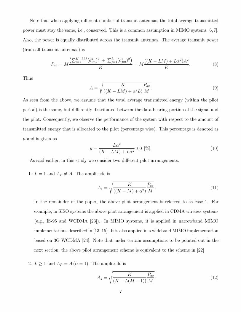
Note that when applying different number of transmit antennas, the total average transmitted
power must stay the same, i.e., conserved. This is a common assumption in MIMO systems [6,7].
Also, the power is equally distributed across the transmit antennas. The average transmit power
(from all transmit antennas) is
Pav = M
(∑K−LMi=1 (ad
im)2 +∑L
j=1(apjm)2
)
K= M
((K − LM) + Lα2)A2
K. (8)
Thus
A =
√K
((K − LM) + α2L)
Pav
M. (9)
As seen from the above, we assume that the total average transmitted energy (within the pilot
period) is the same, but differently distributed between the data bearing portion of the signal and
the pilot. Consequently, we observe the performance of the system with respect to the amount of
transmitted energy that is allocated to the pilot (percentage wise). This percentage is denoted as
µ and is given as
µ =Lα2
(K − LM) + Lα2100 [%]. (10)
As said earlier, in this study we consider two different pilot arrangements:
1. L = 1 and AP 6= A. The amplitude is
A1 =
√K
((K − M) + α2)
Pav
M. (11)
In the remainder of the paper, the above pilot arrangement is referred to as case 1. For
example, in SISO systems the above pilot arrangement is applied in CDMA wireless systems
(e.g., IS-95 and WCDMA [23]). In MIMO systems, it is applied in narrowband MIMO
implementations described in [13–15]. It is also applied in a wideband MIMO implementation
based on 3G WCDMA [24]. Note that under certain assumptions to be pointed out in the
next section, the above pilot arrangement scheme is equivalent to the scheme in [22]
2. L ≥ 1 and AP = A (α = 1). The amplitude is
A2 =
√K
(K − L(M − 1))
Pav
M. (12)
7

In the remainder of the paper, the above pilot arrangement is referred to as case 2. Note that
the above pilot arrangement is frequently used in SISO systems, e.g., wire-line modems [28]
and some wireless standards (e.g., IS-136 and GSM [16]). This arrangement is typically not
used in MIMO systems.
In Section 6 we will analyze the performance of these two cases because they are widely applied
in different communication systems.
3 Estimation of Channel Response
Due to the orthogonality of the pilots and assumption that the elements of H are iid, it can be
shown that to obtain the maximum likelihood estimate of H it is sufficient to estimate hnm (for
m = 1, · · · , M, n = 1, · · · , N), independently1. This is identical to estimating a SISO channel
response between the transmit antenna m and receive antenna n. The estimation is based on
averaging the projections of the received signal on dpjmsp
jm (for j = 1, · · · , L and m = 1, · · · , M) as
hnm =1
LAP
L∑
j=1
(dpjmsp
jm)Hrn
=1
L
L∑
j=1
(hnm + (dpjmsp
jm)Hnn/AP )
= hnm +1
LAP
L∑
j=1
(dpjmsp
jm)Hnn (13)
where hnm denotes the estimate of the channel response hnm. It can be shown that for a frequency-
flat AWGN channel, given the pilot signal and the assumed properties of H, (13) is the maximum-
likelihood estimate of the channel response hnm [17]. The estimation error is
nenm =
1
LAP
L∑
j=1
(dpjmsp
jm)Hnn. (14)
1Based on the above assumptions it can be shown that in this particular case the ML estimate is equal to the
LMMSE estimate considered in [22].
8

Note that nenm corresponds to a Gaussian random variable with distribution N (0, N0/(L (αA)2)).
Thus, the channel matrix estimate H is
H = H + He (15)
where He is the estimation error. Each component of the error matrix He is an independent and
identically distributed random variable nenm given in (14) (where ne
nm is the n-th row and m-th
column element of He).
Having the channel response estimated, the estimate of the transmitted data that is associated
with the temporal signature sdi is obtained starting from the following statistics
zni =1
A(sd
i )Hrn (16)
where the amplitude A is assumed to be known at the receiver. zni corresponds to the n-th
component of the vector
zi = [z1i · · · zNi]T = H di +
1
Ani, i = 1, . . . , K − LM (17)
where the m-th component of di = [ddi1 · · ·d
diM ]T is dd
im (data transmitted from the antenna m and
assigned to the temporal signature sdi ). Further, E[nin
Hi ] = N0 IN×N . It can be shown that zi is
a sufficient statistic for detecting the transmitted data. Using zi a MIMO receiver would perform
detection of the transmitted data. Detection of the spatially multiplexed data which is not a focus
of this paper can be done for example, using the VBLAST algorithm [11, 24].
As a common practice, the detection procedure assumes that the channel response is perfectly
estimated, and that H corresponds to the true channel response. Let us rewrite the expression in
(17) as
zi = (H + He) di +1
Ani − He di = H di +
(1
Ani − He di
). (18)
The effective noise in the detection procedure (as a spatial vector) is
ni =(
1
Ani − He di
). (19)
For the given H, the covariance matrix of the effective noise vector is
Υ = Υ(A) = Eni|H
[ninHi ] =
N0
A2I + E
He|H[HeHe
H] (20)
9

and it is a function of the amplitude A. As said earlier He is a matrix of iid Gaussian random
variables with distribution N (0, N0/(L (αA)2)).
It can be shown that for a Rayleigh channel, where the entries of H are iid Gaussian random
variables with distribution N (0, 1), the above covariance matrix is
Υ =N0
A2I + M
1
1 + L (αA)2/N0I +
(1
1 + L (αA)2/N0
)2
HHH. (21)
4 Estimates Available to Receiver:
Open Loop Capacity
Assuming that the channel response estimate is available to the receiver, only, we determine the
lower bound for the open loop ergodic capacity as follows.
C ≥ R =K − LM
KE
H
[log2 det
(IM×M + HHHΥ−1
)]. (22)
The term (K − LM)/K is introduced because L temporal signature per each transmit antenna
are allocated to the pilot. Also, the random process H has to be stationary and ergodic (this
is a common requirement for fading channel and ergodic capacity [5, 29]). We assume that the
channel coding will span across great number of channel blocks (i.e., we use the well known
infinite channel coding time horizon, required to achieve error-free data transmission with rates
approaching capacity [30]).
In the above expression, equality holds if the effective noise (given in (19)) is AWGN with
respect to the transmitted signal. If the effective noise is not AWGN, then the above rates
represent the worst-case scenario, i.e., the lower bound [22, 31]. In achieving the above rates, the
receiver assumes that the effective noise is interference (which is independent of the transmitted
data) with a Gaussian distribution and spatial covariance matrix Υ. In addition, in the above
expression R represents an achievable rate for reliable transmission (error-free) for the specific
estimation procedure assumed. Knowing the channel response perfectly or using a better channel
estimation scheme (e.g., decision driven schemes) may result in higher achievable rates.
10
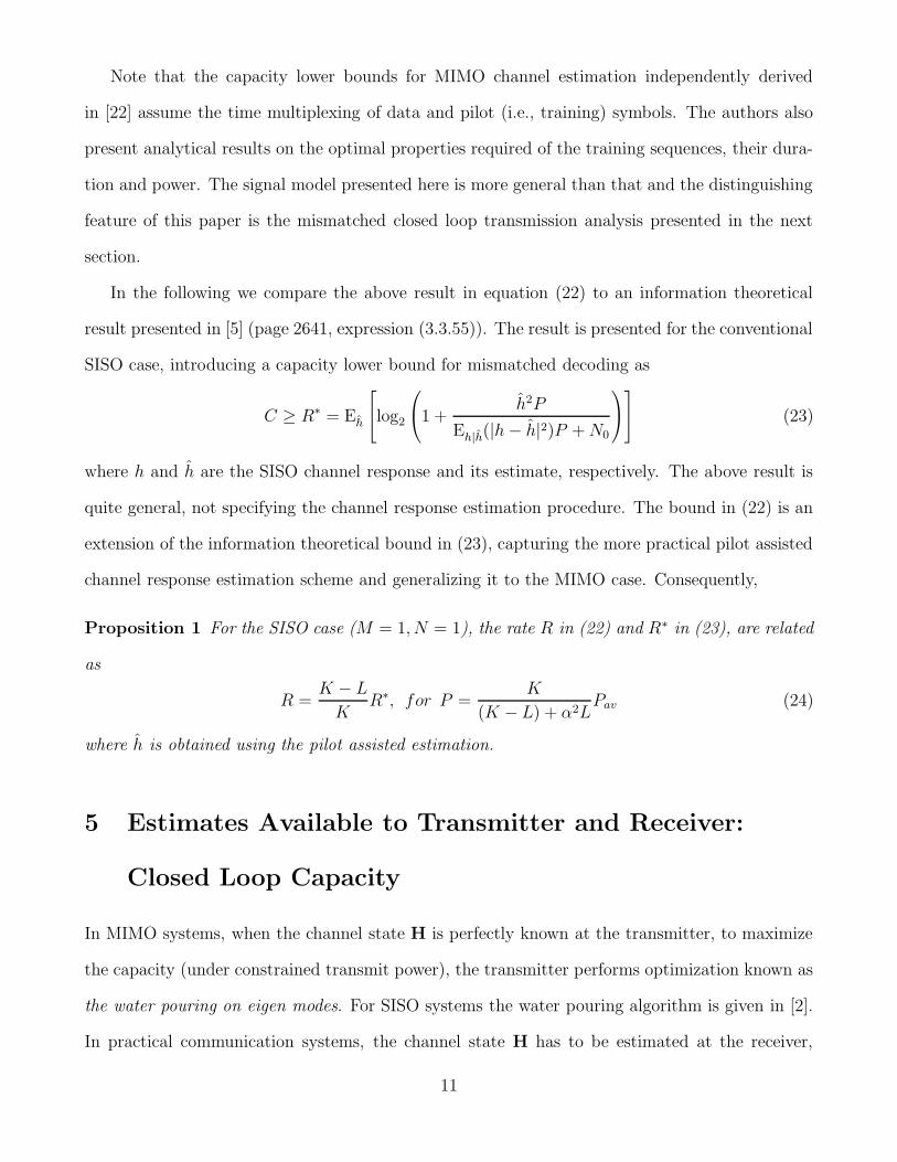
Note that the capacity lower bounds for MIMO channel estimation independently derived
in [22] assume the time multiplexing of data and pilot (i.e., training) symbols. The authors also
present analytical results on the optimal properties required of the training sequences, their dura-
tion and power. The signal model presented here is more general than that and the distinguishing
feature of this paper is the mismatched closed loop transmission analysis presented in the next
section.
In the following we compare the above result in equation (22) to an information theoretical
result presented in [5] (page 2641, expression (3.3.55)). The result is presented for the conventional
SISO case, introducing a capacity lower bound for mismatched decoding as
C ≥ R∗ = Eh
log2
1 +
h2P
Eh|h(|h − h|2)P + N0
(23)
where h and h are the SISO channel response and its estimate, respectively. The above result is
quite general, not specifying the channel response estimation procedure. The bound in (22) is an
extension of the information theoretical bound in (23), capturing the more practical pilot assisted
channel response estimation scheme and generalizing it to the MIMO case. Consequently,
Proposition 1 For the SISO case (M = 1, N = 1), the rate R in (22) and R∗ in (23), are related
as
R =K − L
KR∗, for P =
K
(K − L) + α2LPav (24)
where h is obtained using the pilot assisted estimation.
5 Estimates Available to Transmitter and Receiver:
Closed Loop Capacity
In MIMO systems, when the channel state H is perfectly known at the transmitter, to maximize
the capacity (under constrained transmit power), the transmitter performs optimization known as
the water pouring on eigen modes. For SISO systems the water pouring algorithm is given in [2].
In practical communication systems, the channel state H has to be estimated at the receiver,
11

and then fed to the transmitter. In the case of a time varying channel, this practical procedure
results in noisy and delayed (temporally mismatched) estimates being available to the transmitter
to perform the optimization.
As said earlier, the MIMO channel is time varying. Let Hi−1 and Hi correspond to consecutive
block faded channel responses. In the following, the subscripts i and i−1 on different variables will
indicate values corresponding to the block channel periods i and i− 1, respectively. The temporal
characteristic of the channel is described using the correlation
E[h(i−1)nm h∗
inm
]/Γ = κ, (25)
where Γ = E[hinmh∗inm], and hinm is a stationary random process (for m = 1, · · · , M and n =
1, · · · , N , denoting transmit and receive antenna indices, respectively). We assume that the knowl-
edge of the correlation κ is not known at the receiver and the transmitter. Note that the above
channel is modeled as a first order discrete Markov process2.
Adopting a practical scenario, we assume that the receiver feeds back the estimate Hi−1.
Because the ideal channel state Hi is not available at the transmitter, we assume that Hi−1 is
used instead to perform the water pouring transmitter optimization for the i-th block. In other
words the transmitter is ignoring the fact that Hi 6= Hi−1.
The water pouring optimization is performed as follows. First, the estimate is decomposed
using singular value decomposition (SVD) as Hi−1 = Ui−1Σi−1VHi−1 [32]. Then, if the data vector
d(k) is to be transmitted (in equation (4)), the following linear transformation is performed at
the transmitter
d(k) = Vi−1Sid(k), (26)
where the matrix Si is a diagonal matrix whose elements sijj (j = 1, · · ·M) are determined by the
water pouring algorithm per singular value of Hi−1, i.e., the diagonal element of Σi−1 (denoted as
2Note that in the case of Jake’s model, κ = J0(2πfdτ), where fd is the maximum Doppler frequency and τ is
the time difference between h(i−1)nm and hinm.
12

σ(i−1)jj , j = 1, · · ·M). The diagonal element of Si is defined as
s2ijj =
1γ0
− N0
|σ(i−1)jj |2A2 for |σ(i−1)jj|2A2 ≥ γ0
0 otherwise(27)
γ0 is a cut-off value, and it depends on the channel fading statistics. It is selected such that the
average transmit power stays the same Pav [2]. Consequently, at the time instant k the received
spatial vector is
y(k) = HiVi−1Sid(k) + Hip(k) + n(k) = Gd(k) + Hip(k) + n(k) (28)
and
G = HiVi−1Si. (29)
The water pouring optimization is applied on the data bearing portion of the signal d(k), while
the pilot p(k) is not changed. The receiver knows that the transformation in (26) is performed
at the transmitter. The receiver performs estimation of the channel response matrix as given in
section 3, resulting in G = HiVi−1Si and the error matrix Ge = HeiVi−1Si. In this case, the
effective noise in (19) and its covariance matrix in (20) are modified accordingly resulting in
ΥWP = ΥWP (A) =N0
A2I + E
Ge|G[GeGe
H]. (30)
In the above and following expressions the superscript ”WP” denotes water pouring. Note that
the above application of the water pouring algorithm per eigen mode is suboptimal, i.e., it is
mismatched (because Hi−1 is used instead of Hi). Consequently, the closed loop system capacity
is bounded as,
CWP ≥ RWP =K − LM
KE
G
[log2 det
(IM×M + GGH(ΥWP )−1
)]. (31)
Similar to the comments related to the result in (22), the random process G has to be stationary
and ergodic. Also, the channel coding will span across infinite number of channel blocks to achieve
error-free data transmission approaching the above rates. Again, the equality holds if the effective
noise is AWGN with respect to the transmitted signal and if not, then the above rates represent the
13
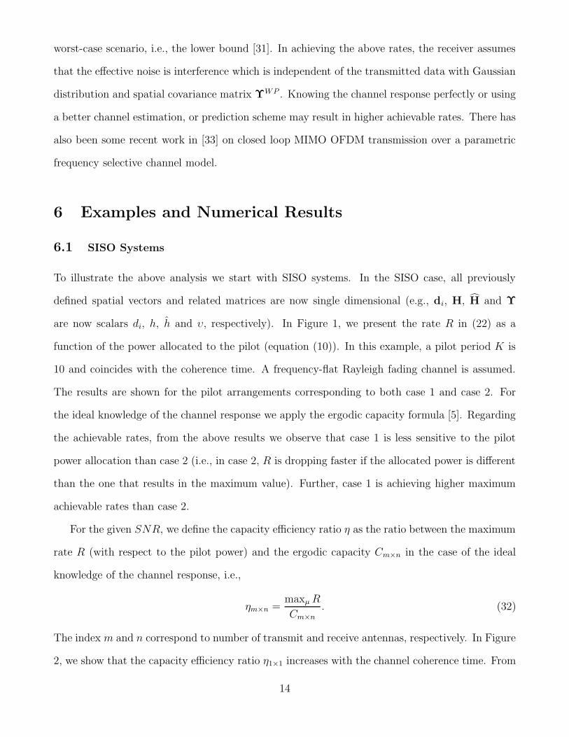
worst-case scenario, i.e., the lower bound [31]. In achieving the above rates, the receiver assumes
that the effective noise is interference which is independent of the transmitted data with Gaussian
distribution and spatial covariance matrix ΥWP . Knowing the channel response perfectly or using
a better channel estimation, or prediction scheme may result in higher achievable rates. There has
also been some recent work in [33] on closed loop MIMO OFDM transmission over a parametric
frequency selective channel model.
6 Examples and Numerical Results
6.1 SISO Systems
To illustrate the above analysis we start with SISO systems. In the SISO case, all previously
defined spatial vectors and related matrices are now single dimensional (e.g., di, H, H and Υ
are now scalars di, h, h and υ, respectively). In Figure 1, we present the rate R in (22) as a
function of the power allocated to the pilot (equation (10)). In this example, a pilot period K is
10 and coincides with the coherence time. A frequency-flat Rayleigh fading channel is assumed.
The results are shown for the pilot arrangements corresponding to both case 1 and case 2. For
the ideal knowledge of the channel response we apply the ergodic capacity formula [5]. Regarding
the achievable rates, from the above results we observe that case 1 is less sensitive to the pilot
power allocation than case 2 (i.e., in case 2, R is dropping faster if the allocated power is different
than the one that results in the maximum value). Further, case 1 is achieving higher maximum
achievable rates than case 2.
For the given SNR, we define the capacity efficiency ratio η as the ratio between the maximum
rate R (with respect to the pilot power) and the ergodic capacity Cm×n in the case of the ideal
knowledge of the channel response, i.e.,
ηm×n =maxµ R
Cm×n
. (32)
The index m and n correspond to number of transmit and receive antennas, respectively. In Figure
2, we show that the capacity efficiency ratio η1×1 increases with the channel coherence time. From
14
the above results we conclude that case 1 is a more efficient scheme than case 2.
6.2 MIMO Systems
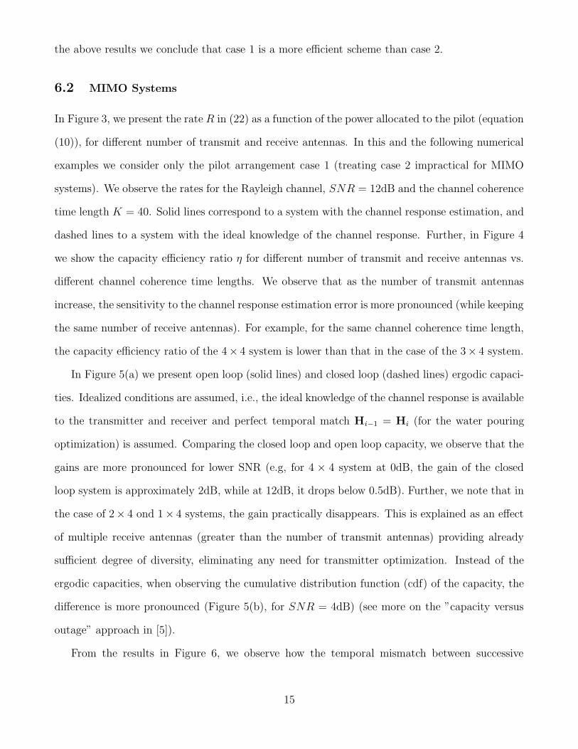
In Figure 3, we present the rate R in (22) as a function of the power allocated to the pilot (equation
(10)), for different number of transmit and receive antennas. In this and the following numerical
examples we consider only the pilot arrangement case 1 (treating case 2 impractical for MIMO
systems). We observe the rates for the Rayleigh channel, SNR = 12dB and the channel coherence
time length K = 40. Solid lines correspond to a system with the channel response estimation, and
dashed lines to a system with the ideal knowledge of the channel response. Further, in Figure 4
we show the capacity efficiency ratio η for different number of transmit and receive antennas vs.
different channel coherence time lengths. We observe that as the number of transmit antennas
increase, the sensitivity to the channel response estimation error is more pronounced (while keeping
the same number of receive antennas). For example, for the same channel coherence time length,
the capacity efficiency ratio of the 4× 4 system is lower than that in the case of the 3× 4 system.
In Figure 5(a) we present open loop (solid lines) and closed loop (dashed lines) ergodic capaci-
ties. Idealized conditions are assumed, i.e., the ideal knowledge of the channel response is available
to the transmitter and receiver and perfect temporal match Hi−1 = Hi (for the water pouring
optimization) is assumed. Comparing the closed loop and open loop capacity, we observe that the
gains are more pronounced for lower SNR (e.g, for 4 × 4 system at 0dB, the gain of the closed
loop system is approximately 2dB, while at 12dB, it drops below 0.5dB). Further, we note that in
the case of 2× 4 ond 1× 4 systems, the gain practically disappears. This is explained as an effect
of multiple receive antennas (greater than the number of transmit antennas) providing already
sufficient degree of diversity, eliminating any need for transmitter optimization. Instead of the
ergodic capacities, when observing the cumulative distribution function (cdf) of the capacity, the
difference is more pronounced (Figure 5(b), for SNR = 4dB) (see more on the ”capacity versus
outage” approach in [5]).
From the results in Figure 6, we observe how the temporal mismatch between successive
15

channel responses (Hi−1 6= Hi) affects the achievable rates RWP in (31). As said earlier, the
temporal mismatch is characterized by the correlation E[h(i−1)nm h∗
inm
]/Γ = κ (for m = 1, · · · , M
and n = 1, · · · , N). We observe the cases when the ideal channel response (dashed lines) and
channel response estimates (solid lines) are available at the transmitter and the receiver. Solid
lines correspond to the channel response estimation where the pilot power is selected to maximize
the achievable rate RWP . We observe the rates for the Rayleigh channel, SNR = 4dB and the
coherence time length K = 40. Note that for κ = 0 (i.e., when the successive channel responses
are uncorrelated), the achievable rate is lower than in the case of κ = 1 (i.e., when the successive
channel responses are fully correlated). The drop in the achievable rates is not substantial, even
though the water pouring algorithm is fully mismatched for κ = 0. We explain this behavior in
the following. In the case of a Rayleigh channel, the matrix Vi−1Si usually has M degrees of
freedom, and a small condition number of the corresponding covariance matrix. Consequently,
even in the mismatched case, multiplying Hi with Vi−1Si preserves the degrees of freedom of
the matrix Hi resulting in a high capacity of the composite channel G in (29). We expect the
detrimental effects of the mismatch to be amplified in the case of Rician channels, especially those
with large K-factor. This is because Rician channels result in the matrix Vi−1Si having a few
dominant degrees of freedom there by making accurate feedback beneficial.
In Figure 7 we compare the open loop scheme to the closed loop scheme under temporal
mismatch. It is observed that when the channel coherence is low (i.e., low correlation κ), it is
better to not use a closed loop scheme. In the observed case (4 × 4, SNR = 4dB and coherence
time K = 40), for the correlation coefficient κ < 0.7 the achievable rates for the closed loop scheme
are lower than in the open loop case.
7 Conclusion
In this paper we have studied how the estimation error of the frequency-flat time-varying channel
response affects the performance of a MIMO communication system. Using a block-fading channel
model, we have connected results of information theory with practical pilot estimation for such
16

systems. The presented analysis may be viewed as a study of mismatched receiver and transmitter
algorithms in MIMO systems. We have considered two pilot based schemes for the estimation. The
first scheme uses a single pilot symbol per block with different power than the data symbol power.
The second scheme uses more than one pilot symbol per block, whose power is the same as the
data symbol power. We have presented how the achievable data rates depend on the percentage
of the total power allocated to the pilot, background noise level and the channel coherence time
length. Our results have shown that the first pilot-based approach is less sensitive to the fraction
of power allocated to the pilot. Furthermore, we have observed that as the number of transmit
antennas increase, the sensitivity to the channel response estimation error is more pronounced
(while keeping the same number of receive antennas). The effects of the estimation error are
evaluated in the case of the estimates being available at the receiver only (open loop), and in
the case when the estimates are fed back to the transmitter (closed loop) allowing water pouring
transmitter optimization. In the case of water pouring transmitter optimization and corresponding
rates, we have not observed significant gains versus the open loop rates for the channel models
considered here. Further, we observe in certain cases, it is better to use the open loop scheme
as opposed to the closed loop scheme. The analysis presented here can be used to optimally
allocate pilot power for various system and channel operating conditions, and to also determine
the effectiveness of closed loop feedback.
Acknowledgments
The authors would like to thank Dr. Gerard Foschini and Dr. Dimitry Chizhik for their construc-
tive comments and valuable discussions.
References
[1] G. J. Foschini and J. Salz, “Digital Communications over Fading Radio Channels,” Bell Labs Tech-
nical Journal, pp. 429–456, February 1983.
17

[2] A. Goldsmith and P. Varaiya, “Increasing Spectral Efficiency Through Power Control,” ICC, vol. 1,
pp. 600–604, 1993.
[3] G. Caire, G. Taricco, and E. Biglieri, “Optimum Power Control Over Fading Channels,” IEEE
Transactions on Information Theory, vol. 45, pp. 1468 –1489, July 1999.
[4] L. Song and N. Mandayam, “Hierarchical SIR and Rate Control on the Forward Link for CDMA
Data Users Under Delay and Error Constraints,” IEEE JSAC, vol. 19, pp. 1871 –1882, October
2001.
[5] E. Biglieri, J. Proakis, and S. Shamai, “Fading channels: Information-Theoretic and Communications
Aspects,” IEEE Transactions on Information Theory, vol. 44, pp. 2619 –2692, October 1998.
[6] G. J. Foschini, “Layered Space-Time Architecture for Wireless Communication in a Fading Envi-
ronment When Using Multiple Antennas,” Bell Labs Technical Journal, vol. 1, no. 2, pp. 41–59,
1996.
[7] G. J. Foschini and M. J. Gans, “On Limits of Wireless Communications in a Fading Environment
when Using Multiple Antennas,” Wireless Personal Communications, no. 6, pp. 315–335, 1998.
[8] D. Chizhik, G. J. Foschini, M. J. Gans, and R. Valenzuela, “Keyholes, Correlations, and Capacities
of Multielement Transmit and Receive Antennas,” IEEE Transactions on Wireless Communications,
vol. 1, pp. 361–368, April 2002.
[9] D. Chizhik, J. Ling, P. W. Wolniansky, R. A. Valenzuela, N. Costa, and K. Huber, “Multiple Input
Multiple Output Measurements and Modeling in Manhattan,” VTC Fall, vol. 1, pp. 107–110, 2002.
[10] P. Soma, D. S. Baum, V. Erceg, R. Krishnamoorthy, and A. Paulraj, “Analysis and Modeling of
Multiple-Input Multiple-Output (MIMO) Radio Channel Based on Outdoor Measurements Con-
ducted at 2.5 GHz for Fixed BWA Applications,” IEEE Conference ICC 2002, pp. 272 – 276, 2002.
[11] G. J. Foschini, G. D. Golden, R. A. Valenzuela, and P. W. Wolniansky, “Simplified Processing
for Wireless Communications at High Spectral Efficiency,” IEEE JSAC, vol. 17, pp. 1841–1852,
November 1999.
18

[12] D. Samardzija, P. Wolniansky, and J. Ling, “Performance Evaluation of the VBLAST Algorithm
in W-CDMA Systems,” The IEEE Vehicular Technology Conference (VTC), vol. 2, pp. 723–727,
September 2001. Atlantic City.
[13] G. D. Golden, G. J. Foschini, R. A. Valenzuela, and P. W. Wolniansky, “Detection Algorithm and
Initial Laboratory Results using V-BLAST Space-Time Communication Architecture,” Electronics
Letters, vol. 35, pp. 14–16, January 1999.
[14] H. Zheng and D. Samardzija, “Performance Evaluation of Indoor Wireless System Using BLAST
Testbed,” The IEEE Vehicular Technology Conference (VTC), vol. 2, pp. 905–909, October 2001.
Atlantic City.
[15] D. Samardzija, C. Papadias, and R. A. Valenzuela, “Experimental Evaluation of Unsupervised Chan-
nel Deconvolution for Wireless Multiple-Transmitter/Multiple-Receiver Systems,” Electronic Letters,
pp. 1214–1215, September 2002.
[16] G. L. Stuber, Principles of Mobile Communications. Kluwer Academic Publishers, first ed., 1996.
[17] H. V. Poor, An Introduction to Signal Detection and Estimation. Springer-Verlag, second ed., 1994.
[18] A. Lapidoth and S. Shamai, “Fading Channels: How Perfect Need ”Perfect Side Information” Be?,”
IEEE Transaction on Information Theory, vol. 48, pp. 1118 –1134, May 2002.
[19] S. Shamai and T. Marzetta, “Multiuser Capacity in Block Fading With No Channel State Informa-
tion,” IEEE Transaction on Information Theory, vol. 48, pp. 938 –942, April 2002.
[20] T. L. Marzetta, “Blast Training: Estimating Channel Characteristics for High-Capacity Space-
Time Wireless,” 37th Annual Allerton Conference on Communications, Control and Computing,
September 1999.
[21] J. Baltersee, G. Fock, and H. Meyr, “Achievable Rate of MIMO Channels With Data-Aided Channel
Estimation and Perfect Interleaving,” IEEE JSAC, vol. 19, pp. 2358–2368, December 2001.
[22] B. Hassibi and B. M. Hochwald, “How Much Training is Needed in Multiple-Antenna Wireless
Links,” Technical Memorandum, Bell Laboratories, Lucent Technologies, October 2001.
19

[23] H. Holma and A. Toskala, eds., WCDMA for UMTS. Wiley, first ed., 2000.
[24] A. Burg, E. Beck, D. Samardzija, M. Rupp, and et al., “Prototype Experience for MIMO BLAST over
Third Generation Wireless System,” IEEE JSAC Special Issue on MIMO Systems and Applications,
vol. 21, April 2003.
[25] J. C. Guey, M. P. Fitz, M. R. Bell, and W. Kuo., “Signal Design for Transmitter Diversity Wire-
less Communication Systems over Rayleigh Fading Channels,” Proc. of IEEE Vehicular Technology
Conference, vol. 1, pp. 136–140, 1996. Atlanta.
[26] J. C. Guey, M. P. Fitz, M. R. Bell, and W. Y. Kuo, “Signal Design for Transmitter Diversity Wireless
Communication Systems over Rayleigh Fading Channels,” IEEE Transactions on Communications,
vol. 47, pp. 527–537, 1999.
[27] D. Shiu, G. J. Foschini, and M. J. Gans, “Fading Correlation and Its Effects on the Capacity of
Multielement Antenna Systems,” IEEE Transactions on Communications, vol. 48, pp. 502 –513,
March 2000.
[28] J. G. Proakis, Digital Communications. New York: McGraw-Hill, 3rd ed., 1995.
[29] L. Li and A. Goldsmith, “Capacity and Optimal Resource Allocation for Fading Broadcast Channels
- Part I: Ergodic Capacity,” Information Theory, IEEE Transactions, vol. 47, pp. 1083–1102, March
2001.
[30] J. M. Wozencraft and I. M. Jacobs, Principles of Communication Engineering. New York: Wiley,
1965.
[31] R. G. Gallager, Information Theory and Reliable Communications. New York: John Wiley and Sons,
1968.
[32] G. Strang, Linear Algebra and its Applications. Harcourt Brace Jovanovich, third ed., 1988.
[33] C. Wen, Y. Wang, and J. Chen, “Adaptive Spatio-Temporal Coding Scheme for Indoor Wireless
Communication,” IEEE JSAC, vol. 21, pp. 161–170, February 2003.
20

0 10 20 30 40 50 60 70 80 90 1000
1
2
3
4
5
6
Rat
e[bi
ts/s
ymbo
l]
Pilot power [%]
Ideal channel knowledgeWith estimation: case 1With estimation: case 2
20 dB
12 dB
4 dB
Figure 1: Achievable open loop rates vs. power allocated to the pilot, SISO system, SNR =
4, 12, 20dB, coherence time K = 10, Rayleigh channel.
21

10 20 30 40 50 60 70 80 90 1000.7
0.75
0.8
0.85
0.9
0.95
1
Cap
acity
effi
cien
cy r
atio
Channel coherence time [sample periods]
Case 1, SNR = 20dBCase 1, SNR = 4dBCase 2, SNR = 20dBCase 2, SNR = 4dB
Figure 2: Capacity efficiency ratio vs. channel coherence time (K = 10, 20, 40, 100), SISO system,
SNR = 4, 20dB, Rayleigh channel.
22

0 10 20 30 40 50 60 70 80 90 1000
2
4
6
8
10
12
14
Rat
e[bi
ts/s
ymbo
l]
Pilot power [%]
4x43x42x41x41x1
Figure 3: Achievable open loop rates vs. power allocated to the pilot, MIMO system, SNR =
12dB, coherence time K = 40, Rayleigh channel, solid line corresponds to a system with the
channel response estimation, and dashed line to the case of the ideal channel response knowledge.
23

10 20 30 40 50 60 70 80 90 100
0.5
0.6
0.7
0.8
0.9
1
Cap
acity
effi
cien
cy r
atio
Channel coherence time [sample periods]
4x43x42x41x41x1
Figure 4: Capacity efficiency ratio vs. channel coherence time (K = 10, 20, 40, 100), MIMO
system, SNR = 12dB, Rayleigh channel.
24

0 2 4 6 8 10 12 14 160
2
4
6
8
10
12
14
16
18
Cap
acity
[bits
/sym
bol]
SNR[dB]
4x43x42x41x41x1
(a) Ergodic capacity vs. SNR, MIMO system, ideal knowledge of the channel response, Rayleigh channel,
solid line corresponds to open loop capacity, and dashed line to closed loop capacity (perfect temporal
match Hi−1 = Hi is assumed).
0 1 2 3 4 5 6 7 8 9 100
0.1
0.2
0.3
0.4
0.5
0.6
0.7
0.8
0.9
1
Rate[bits/symbol]
Pro
babi
lity
4x4 1x4 1x1
Figure 5: (b) CDF of capacity, MIMO system, SNR = 4dB, ideal knowledge of the channel response,
Rayleigh channel, solid line corresponds to open loop capacity, and dashed line to closed loop capacity
(perfect temporal match Hi−1 = Hi is assumed).
25

0 0.1 0.2 0.3 0.4 0.5 0.6 0.7 0.8 0.9 11
2
3
4
5
6
7
Rat
e[bi
ts/s
ymbo
l]
Successive channel response correlation
4x43x42x41x41x1
Figure 6: Achievable closed loop rates vs. correlation between successive channel responses, MIMO
system, SNR = 4dB, coherence time K = 40, Rayleigh channel, solid line corresponds to a system
with the channel response estimation, and dashed line to the case of the ideal channel response
available at the transmitter and the receiver (but with the temporal mismatched Hi−1 6= Hi).
26

0 0.1 0.2 0.3 0.4 0.5 0.6 0.7 0.8 0.9 13.5
4
4.5
5
5.5
6
6.5
7
Rat
e[bi
ts/s
ymbo
l]
Successive channel response correlation
4x4, closed loop4x4, open loop
Figure 7: Achievable closed loop and open loop rates vs. correlation between successive channel
responses, MIMO system 4 × 4, SNR = 4dB, coherence time K = 40, Rayleigh channel, solid
line corresponds to a system with the channel response estimation, and dashed line to the case of
the ideal channel response available at the transmitter and the receiver (but with the temporal
mismatched Hi−1 6= Hi).
27