piezoelectric-based in-situ damage detection of composite
TRANSCRIPT
Piezoelectric-Based In-Situ Damage Detection of Composite Materials for Structural Health Monitoring Systems
by
Seth Stovack Kessler
S.M. Aeronautics and Astronautics
Massachusetts Institute of Technology, 2/2000
S.B. Aeronautics and Astronautics Massachusetts Institute of Technology, 6/1998
Submitted to the Department of Aeronautics and Astronautics in Partial Fulfillment of the Requirements for the Degree of
DOCTORATE OF PHILOSOPHY IN AERONAUTICS AND ASTRONAUTICS
AT THE MASSACHUSETTS INSTITUTE OF TECHNOLOGY
FEBRUARY 2002
2002 Seth Stovack Kessler
Signature of Author………………………………………………………………………...…………………………. Department of Aeronautics and Astronautics
Massachusetts Institute of Technology January 28th, 2002
Certified by……………………………………………………………….……………………………………...……..
S. Mark Spearing Associate Professor of Aeronautics and Astronautics
Massachusetts Institute of Technology Thesis Committee Chairman
Certified by……………………………………………………………….…………………………………………..... Carlos E. S. Cesnik
Associate Professor of Aerospace Engineering The University of Michigan Thesis Committee Member
Certified by……………………………………………………………….……………………………………………. Mauro J. Atalla
Research Engineer, United Technologies Research Center Thesis Committee Member
Certified by……………………………………………………………….…………………………………………….
Marthinus van Schoor President, Midé Technology Corporation
Thesis Committee Member
Accepted by…………………………………………………………….………………………………………………. Wallace E. Vander Velde
Professor of Aeronautics and Astronautics Massachusetts Institute of Technology Chair, Committee on Graduate Students

2
[This page intentionally left blank]
3
PIEZOELECTRIC-BASED IN-SITU DAMAGE DETECTION OF COMPOSITE MATERIALS FOR STRUCTURAL
HEALTH MONITORING SYSTEMS
by
Seth Stovack Kessler
Submitted to the Department of Aeronautics and Astronautics on January 28th, 2002 in partial fulfillment of the
requirements for the Degree of Doctorate of Philosophy in Aeronautics and Astronautics
ABSTRACT
Cost-effective and reliable damage detection is critical for the utilization of composite materials. This thesis presents the conclusions of an analytical and experimental survey of candidate methods for in-situ damage detection in composite materials. Finite element results are presented for the application of modal analysis and Lamb wave techniques to quasi-isotropic graphite/epoxy test specimens containing representative damage. These results were then verified experimentally by using piezoelectric patches as actuators and sensors for both sets of experiments. The passive modal analysis method was reliable for detecting small amounts of global damage in a simple composite structures. By comparison, the active Lamb wave method was sensitive to all types of local damage present between the sensor and actuator, provided useful information about damage presence and severity, and presents the possibility of estimating damage type and location. Analogous experiments were also performed for more complex built-up structures such as sandwich beams, stiffened plates and composite cylinders. These techniques have proven suitable for structural health monitoring applications since they can be applied with low power conformable sensors and can provide useful information about the state of a structure during operation. Piezoelectric patches could also be used as multipurpose sensors to test using a variety of methods such as modal analysis, Lamb wave, acoustic emission and strain based methods simultaneously by altering driving frequencies and sampling rates. Guidelines and recommendations drawn from this research are presented to assist in the design of a structural health monitoring system for a vehicle, and provides a detailed example of a SHM system architecture. These systems will be an important component in future designs of air and spacecraft to increase the feasibility of their missions. Thesis Supervisor: S. Mark Spearing Title: Associate Professor of Aeronautics and Astronautics

4
ACKNOWLEDGMENTS
There are many people I would like to recognize for their help and support with my
research. Without them, I would not have been able to accomplish this milestone so quickly with
such satisfying results. I would like to thank my advisor Prof. Mark Spearing; he has always
believed in my abilities and provided whatever advice and resources necessary for me to
accomplish my goals. The rest of my thesis committee, Prof. Carlos Cesnik, Dr. Mauro Atalla
and Dr. Tienie van Schoor, each spent countless hours meeting with me to discuss aspects of my
research and working revisions of my various publications. While not officially a member of my
thesis committee, Prof. Costas Soutis provided as much support as anyone else during the past
few years, and added much more meaning to my work.
Next, I would like to acknowledge everyone who provided technical support for this
project. Thanks to Al Supple for teaching me almost everything I know about composite
manufacturing, and John Kane, Don Weiner for provided invaluable assistance with testing and
machining throughout my the project. A special thanks goes to Dave Robertson, who spent
much of his free time assisting me with electrical components for my experiments. Prof. Paul
Lagace, Prof. John Dugundji and Prof. S.C. Wooh have also provided me with valuable advice.
Many co-workers contributed to this work by helping with research, analysis, writing
and providing support. Thank you DJ, Torrey, Chris, Jeremy Mark, Barb and Dennis from
TELAC, Erin from GTL, and Kevin, Chris and Dave from AMSL who have given me wonderful
advice, inspiration and friendship over the years. A special thanks goes to all of my UROP’s:
Ricky Watkins, Michelle Park, Joel Torres.
Lastly, I need to thank my loving family—Dad, Mom, Bree and Moira—who have
always given me their support. I love you all.

5
Table of Contents
1. INTRODUCTION ................................................................................................................... 11
2. BACKGROUND ..................................................................................................................... 15
2.1 Non-Destructive Evaluation (NDE) in Composite Materials ....................................... 15 2.1.1 Visual inspection methods........................................................................................................................... 16 2.1.2 X-radiography methods................................................................................................................................ 17 2.1.3 Strain gauge methods.................................................................................................................................... 18 2.1.4 Optical fiber methods.................................................................................................................................... 18 2.1.5 Ultrasonic methods........................................................................................................................................ 19 2.1.6 Eddy current methods................................................................................................................................... 20 2.1.7 Vibration-based methods.............................................................................................................................. 20 2.1.8 Other methods................................................................................................................................................ 22
2.2 Current Inspection Regulations and Practices .............................................................. 22
2.3 Structural Health Monitoring ........................................................................................ 24
2.3.1 Motivations for SHM .................................................................................................................................... 25 2.3.2 General SHM applications........................................................................................................................... 30 2.3.3 SHM in composite structures....................................................................................................................... 33 2.3.4 Goals for SHM ............................................................................................................................................... 34
3. FREQUENCY RESPONSE METHODS ................................................................................ 35
3.1 Background ................................................................................................................... 35
3.1.1 Model-based frequency response methods................................................................................................ 36 3.1.2 Model independent frequency response methods.................................................................................... 38
3.2 Analytical Procedures ................................................................................................... 39
3.2.1 Simple beam theory ....................................................................................................................................... 39 3.2.2 Finite element modeling ............................................................................................................................... 40
3.3 Experimental Procedures .............................................................................................. 41
3.3.1 Specimen fabrication..................................................................................................................................... 42 3.3.2 Laser vibrometer tests ................................................................................................................................... 43 3.3.3 Impedance tests .............................................................................................................................................. 43
3.4 Results ........................................................................................................................... 44 3.4.1 Analytical results ........................................................................................................................................... 44 3.4.2 Experimental results...................................................................................................................................... 45
3.5 Discussion..................................................................................................................... 46 3.5.1 Effect of damage on frequency response................................................................................................... 46 3.5.2 Comparison of analytical and experimental results ................................................................................. 48 3.5.3 Role of frequency response methods in SHM .......................................................................................... 49
3.6 Conclusions ................................................................................................................... 51
6
4. LAMB WAVE METHODS..................................................................................................... 59
4.1 Background ................................................................................................................... 59 4.1.1 Early Lamb wave theory and applications ................................................................................................ 60 4.1.2 Lamb waves in composite materials ........................................................................................................... 62
4.2 Analytical Procedures ................................................................................................... 63 4.2.1 Dispersion curve formulation ...................................................................................................................... 63 4.2.2 Propagation and limitations of Lamb waves ............................................................................................. 65 4.2.3 Finite element modeling ............................................................................................................................... 67
4.3 Optimization Procedures............................................................................................... 69
4.3.1 Frequency selection....................................................................................................................................... 69 4.3.2 Pulse shape selection..................................................................................................................................... 71 4.3.3 Actuator selection.......................................................................................................................................... 73 4.3.4 Signal interpretation ...................................................................................................................................... 74
4.4 Experimental Procedures .............................................................................................. 77 4.4.1 Narrow coupon tests ...................................................................................................................................... 77 4.4.2 Sandwich beam tests ..................................................................................................................................... 79 4.4.3 Stiffened plate tests........................................................................................................................................ 79 4.4.4 Composite sandwich cylinder tests............................................................................................................. 80 4.4.5 2-D plate tests ................................................................................................................................................. 81 4.4.6 Self-sensing tests............................................................................................................................................ 82
4.5 Results ........................................................................................................................... 82
4.5.1 Analytical results ........................................................................................................................................... 83 4.5.2 Experimental results...................................................................................................................................... 85
4.6 Discussion..................................................................................................................... 86
4.6.1 Effect of damage on Lamb waves............................................................................................................... 87 4.6.2 Comparison of analytical and experimental results ................................................................................. 89 4.6.3 Role of Lamb wave methods in SHM ........................................................................................................ 91
4.7 Conclusions ................................................................................................................... 92
5. OTHER PIEZOELECTRIC-BASED SENSING METHODS .............................................. 115
5.1 Background ................................................................................................................. 116
5.2 Narrow Coupon Tensile Tests .................................................................................... 118
5.2.1 Acoustic emission results ........................................................................................................................... 119 5.2.2 Strain monitoring results ............................................................................................................................ 120
5.3 2-D Plate Tests............................................................................................................ 121
5.4 Discussion................................................................................................................... 122
7
6. STRUCTURAL HEALTH MONITORING SYSTEMS....................................................... 129
6.1 Components of SHMS ................................................................................................ 129
6.1.1 Architecture .................................................................................................................................................. 130 6.1.2 Damage characterization ............................................................................................................................ 131 6.1.3 Sensors........................................................................................................................................................... 132 6.1.4 Computation ................................................................................................................................................. 133 6.1.5 Communication............................................................................................................................................ 134 6.1.6 Power ............................................................................................................................................................. 135 6.1.7 Algorithms .................................................................................................................................................... 136 6.1.8 Intervention................................................................................................................................................... 136
6.2 Recommendations of Implementation of SHMS in Composite Structures ................ 137
6.3 Future of SHMS.......................................................................................................... 139
7. CONCLUSIONS AND RECOMMENDATIONS ................................................................ 145
7.1 Conclusions ................................................................................................................. 147
7.2 Recommendations for Future Work............................................................................ 149
REFERENCES ........................................................................................................................... 151 APPENDIX A: Mathematica Code for Phase and Group Velocities ..................................... 161 APPENDIX B: Lamb Wave Derivations................................................................................... 164 APPENDIX C: ABAQUS Codes for Frequency Response and Lamb Wave Models ........... 168 APPENDIX D: MATLAB Code for Data Analysis by Wavelet Decomposition .................. 193 APPENDIX E: LabView Codes for Experimental Procedures .............................................. 196

8
List of Figures
Figure 3.1: Diagrams of damage models ..................................................................................... 52
Figure 3.2: Schematic of the delamination modeling procedure ................................................. 52
Figure 3.3: X-Radiographs of damaged specimens ..................................................................... 53
Figure 3.4: Frequency response transfer function plot from FEM in I-DEAS, range 0-20 kHz . 53
Figure 3.5: First four mode shapes of control specimen plotted in I-DEAS ............................... 54
Figure 3.6: Frequency response transfer function plot from I-DEAS, range of 0-500 Hz .......... 54
Figure 3.7: Frequency response plot from scanning laser vibrometer for range of 0-20 kHz..... 55
Figure 3.8: Frequency response plot from impedance meter for full tested range of 0-20 kHz.. 55
Figure 3.9: First four mode shapes of control specimen using laser vibrometer data ................. 56
Figure 3.10: Frequency response plot from vibrometer for all specimens, range of 0-500 Hz... 56
Figure 4.1: Graphical representation of A and S Lamb wave shapes .......................................... 94
Figure 4.2: Phase velocity dispersion curve for the Ao mode of an 8-ply composite laminate .. 94
Figure 4.3: Group velocity dispersion curve for the Ao mode of an 8-ply composite laminate . 95
Figure 4.4: Lamb wave actuation frequency selection flow chart ............................................... 95
Figure 4.5: CFRP specimen (250mm x 50mm) with piezoceramic actuator and sensors ........... 96
Figure 4.6: Actuation signal used to generate Lamb waves, 3.5 sine waves at 15 kHz .............. 96
Figure 4.7: Sandwich beam specimens (250mm x 50mm) with various cores ........................... 97
Figure 4.8: Composite plates (250mm x 250mm) with bonded stiffeners .................................. 97
Figure 4.9: Composite sandwich cylinder with small impacted region....................................... 98
Figure 4.10: 2-D composite plate with four piezoelectric sensors............................................... 98
Figure 4.11: Self-sensing circuit .................................................................................................. 99
Figure 4.12: Preliminary analytical results for 60 kHz signal using Prosper code ...................... 99
Figure 4.13: FEA results for narrow coupon with no damage ................................................... 100
Figure 4.14: FEA results for narrow coupon with 25mm center delamination ......................... 101
Figure 4.15: FEA results for 2-D plate with no stiffener........................................................... 102
Figure 4.16: FEA results for 2-D plate with composite stiffener (no damage) ......................... 103
Figure 4.17: FEA results for 2-D plate with delaminated composite stiffener.......................... 104
Figure 4.18: FEA results for curved sandwich panel with no damage ...................................... 105

9
Figure 4.19: FEA results for curved sandwich panel with impact damage ............................... 106
Figure 4.20: Narrow coupon time-trace of voltage signal from sensor 20 cm from actuator.... 107
Figure 4.21: Sandwich beam time-trace of voltage signal from sensor 20 cm from actuator ... 107
Figure 4.22: Wavelet coefficients for thin coupons; compares 15 kHz energy content ............ 108
Figure 4.23: Wavelet coefficients for beam “blind test”; compares 50 kHz energy content ..... 108
Figure 4.24: Time-trace of voltage signal for stiffened plates, 15 kHz signal........................... 109
Figure 4.25: Wavelet coefficients for stiffened plates; compares 15 kHz energy content ........ 109
Figure 4.26: Time-trace of voltage signal for composite sandwich cylinder, 40 kHz signal .... 110
Figure 4.27: Wavelet coefficients for composite cylinder; compares 40 kHz energy content .. 110
Figure 4.28: Time-trace and wavelet coefficients for circumferential scan, 40 kHz signal ...... 111
Figure 4.29: Time-trace of voltage signal for impacted cylinder, 40 kHz signal ...................... 111
Figure 4.30: Wavelet coefficients for impacted cylinder; compares 40 kHz energy content .... 112
Figure 4.31: Time-trace of voltage signal for 2-D plate, 15 kHz signal.................................... 112
Figure 4.32: Wavelet coefficients for 2-D plate; compares 15 kHz energy content .................. 113
Figure 4.33: Time-trace of voltage signal for self-sensing actuator, 45 kHz signal.................. 113
Figure 5.1: Narrow coupon tensile specimen with strain gauge rosette and piezo sensor......... 124
Figure 5.2: Rotated stress-strain plot for control coupon, piezo voltage data superimposed .... 124
Figure 5.3: Rotated stress-strain plot for coupon with hole, piezo voltage data superimposed 125
Figure 5.4: Acoustic emission setup. Pencil break points for tests #1 and #2 are labeled ....... 125
Figure 5.5: Time-trace of voltage signal recorded by each piezo for tests #1 and #2 ............... 126
Figure 5.6: Wavelet coefficients for acoustic emission tests #1 and #2 .................................... 127
Figure 6.1: Sensor selection space comparing detectable damage size with sensor size .......... 142
Figure 6.2: Sensor selection space comparing detectable damage size with sensor power....... 143

10
List of Tables
Table 3.1: Natural frequencies and mode shapes from FEM in I-DEAS .................................... 57
Table 3.2: Natural frequencies and mode shapes from scanning laser vibrometer data .............. 57
Table 3.3: Natural frequencies from FEM comparing damage in various orientations ............... 57
Table 4.1: Lamb wave times of flight and group velocities for narrow coupons from FEM ..... 114
Table 4.2: Lamb wave times of flight and group velocities for all geometries from FEM ....... 114
Table 4.3: Lamb wave times of flight and group velocitie s for narrow coupons experiments.. 114
Table 4.4: Lamb wave times of flight and group velocities for sandwich beams experiments . 114
Table 6.1: Strengths, limitations and implementation potential for various sensing systems ... 144

11
CHAPTER 1
INTRODUCTION
Structural Health Monitoring (SHM) has been defined in the literature as the “acquisition,
validation and analysis of technical data to facilitate life-cycle management decisions.” [1] More
generally, SHM denotes a system with the ability to detect and interpret adverse “changes” in a
structure in order to improve reliability and reduce life-cycle costs. The most fundamental
challenge in designing a SHM system is knowing what “changes” to look for and how to identify
them. The characteristics of damage in a particular structure plays a key role in defining the
architecture of the SHM system. The resulting “changes,” or damage signature, will dictate the
type of sensors that are required, which in-turn determines the requirements for the rest of the
components in the system.
The present research project focuses on the relationship between various sensors and their
ability to detect “changes” in a material or structure’s behavior. Dozens of sensor types have
been cited throughout the literature such as optical fibers, resistive foil gauges and shape
memory alloys, which detect damage through a variety of techniques—some more effectively
than others. Piezoelectric sensors have become of particular interest in this thesis due to their
versatility, conformability, low power consumption and high bandwidth. Several of these
sensors and sensing methods will be described in detail in future chapters.
Of all the broad applications for SHM, currently the aerospace industry has one of the
highest payoffs since damage can lead to catastrophic (and expensive) failures, and the vehicles

12
involved undergo regular costly inspections. Currently 27% of an average aircraft’s life cycle
cost, both for commercial and military vehicles, is spent on inspection and repair; a figure that
excludes the opportunity cost associated with the time the aircraft is grounded for scheduled
maintenance [2]. These commercial and military vehicles are increasingly using composite
materials to take advantage of their excellent specific strength and stiffness properties, fatigue
performance, as well their ability to reduce radar cross-section and “part-count”. However,
composite materials present challenges for design, manufacturing, maintenance and repair over
metallic parts since they tend to fail by distributed and interacting damage modes [3, 4].
Furthermore, damage detection in composites is more difficult than in metallic structures due to
the anisotropy of the material, the conductivity of the fibers, the insulating properties of the
matrix, and the fact that much of the damage often occurs beneath the top surface of the laminate
and is therefore not readily detectable (the threshold of detectablity is often termed barely visible
impact damage, or BVID). Currently successful composite non-destructive testing (NDT)
techniques for small laboratory specimens, such as X-radiographic detection (penetrant enhanced
X-ray) and hydro-ultrasonics (C-scan), are impractical for in service inspection of large
components and integrated vehicles. Inspection specifications for in-service composite airframes
are published by the FAA, however the listed methods such as eddy-current and single-sided
ultrasound are expensive, time-consuming and can be unreliable when applied to composites by
comparison to techniques used for metals. It is clear that new reliable approaches for damage
detection in composites need to be developed to ensure that the total cost of ownership of critical
structures does not become a limiting factor for their use.
This thesis explores the use of piezoelectric sensors as a means to detect common forms
of damage in graphite/epoxy composite structures. Analytical procedures were used to predict
13
the effectiveness of various testing methods, and to help design and optimize appropriate testing
procedures. Subsequently, these experiments were performed commencing at the narrow coupon
level and building up through representative structural elements. The two primary damage
detection methods explored in the present research were frequency response methods and Lamb
wave techniques. Frequency response methods rely on loss in stiffness in a structure causing a
noticeable shift in the natural frequencies and a corresponding change in the normal mode
shapes. These methods are easily applied and fairly sensitive to damage, however they are often
more practical in detecting global loss of stiffness than localizing the degraded region.
Conversely, Lamb waves, which are a traveling elastic perturbation, can detect small regions of
local damage by observing the wave speed changing due to differences in stiffness in the
damaged zone. The disadvantage of Lamb wave methods is that they require an active driving
mechanism to propagate the waves. Acoustic emission and strain-based methods are also
considered during the course of this work. The overall goal of this project is to create analytical
tools and procedures that are validated by experimentation, in order to make knowledgeable
decisions in designing a reliable SHM system for composite structures using piezoelectric
sensors.
Chapter 2 of this thesis discusses the history of damage detection in structures, assesses
current FAA standard detection practices, and continues to explain the motivations behind
incorporating a structural health monitoring system into a vehicle. In Chapter 3, the
fundamentals of frequency response methods are described, and analytical, computational and
experimental results are presented for the application of these techniques to graphite/epoxy
composite laminates. Similarly, Chapter 4 focuses on Lamb wave methods, introducing their
derivation, finite element solutions and experimental results on simple coupons and built up

14
structures. Both of these chapters discuss the role of their respective methods in future designs
for structural health monitoring systems. Chapter 5 presents two other means of detecting
damage via piezoelectric sensors, and describes experiments performed during the current
research with acoustic emission and strain monitoring methods using PZT piezoceramic sensors.
The cumulative knowledge generated by the previous chapters is then connected in Chapter 6,
which discusses the components of a structural health monitoring system, and then makes
recommendations and provides trade studies to assist in designing a successful in-situ damage
detection system. Finally Chapter 7 provides a summary of the work performed, along with
recommendations for future work in developing SHM systems for composite structures.

15
Chapter 2
BACKGROUND
This chapter presents a survey of damage detection methods for composite materials.
Composite materials are gaining acceptance and demand in several commercial markets
including sporting goods, construction and transportation. For many of these applications
however, such as aircraft, without a reliable damage detection approach, the total cost of
ownership may become a limiting factor for the structure’s use. Several non-destructive
evaluation techniques are compared on the basis of their strengths and weaknesses for in-service
testing of composite materials. Current inspection regulations and practices for composite
components in commercial aircraft are also presented. This chapter concludes with a discussion
of the motivations behind implementing a structural health monitoring system, and background
for various applications presented in the literature.
2.1 Non-Destructive Evaluation (NDE) in Composite Materials
There are several inherent difficulties in detecting damage in composite materials as
opposed to traditional engineering materials such as metals or plastics. One reason is due to its
inhomogeneity and anisotropy; most metals and plastics are formed by one type of uniformly
isotropic material with very well known properties. Laminated composite materials on the other
hand can have a widely varying set of material properties based on the chosen fibers, matrix and

16
manufacturing process. This makes modeling composites complex, and often non-linear.
Another obstacle to many detection techniques is the fact that composites are often a mix
between materials with widely differing properties, such as a very good conducting fiber in an
insulating matrix. A last difficulty is that damage in composite materials often occurs below the
surface, which further prevents the implementation of several detection methods. The
importance of damage detection for composite structures is often accentuated over that of
metallic or plastic structures because of their load bearing requirements. Typically unreinforced
plastics are not used in load critical members; since their properties are predictable and are
usually simple and inexpensive to manufacture, they are often designed to be replaceable safe-
life parts. Similarly, metals are generally well understood and easy to model, thus they are
frequently designed using damage tolerant methodologies. The behavior of composite material
on the other hand is much less well understood, and an unexpected failure of the composite part
could prove catastrophic to a vehicle. These materials are still often used in many structures
however, mostly for applications where high specific strength and stiffness are required.
Therefore, the development of reliable damage detection methods is critical to maintain the
integrity of these vehicles. The following sections provide descriptions of various non-
destructive techniques that have been developed for the detection of damage in composite
materials [5].
2.1.1 Visual inspection methods
Perhaps the most natural form of evaluating composite materials is by visual inspection
[6]. Several variants of this method exist at various levels of sophistication from the use of a
static optical or scanning electron microscope to optical examination by eye over the structure.

17
While microscopy can be a useful method to obtain detailed information such as micro-crack
counting or delamination area, it can only be used in the laboratory since a section must be
removed from the larger structure. Visual inspection of a vehicle is perhaps the simplest and
least expensive method described in this section, however often damage in composite materials
occurs below the surface, so it is not easy to identify by the unassisted eye. Also, the eye alone
can determine little detail about the damage mechanism or its severity. While this method can
potentially provide some useful data for damage detection, on a large-scale structure this process
would prove inefficient and ineffective.
2.1.2 X-radiography methods
X-radiographic techniques rely on recording the difference in x-ray absorption rates
through the surface of a structure. These methods can be implemented in real-time digitally, or
by taking static radiographs, whereas areas of different permeability or density are differentiated
by the magnitude of x-ray exposure to the media on the opposite side of the surface after a
predetermined excitation time. To accentuate damaged regions with cracks or delamination,
often a liquid penatrant is applied to the area to be examined. While these techniques are
relatively inexpensive and simple to implement and interpret, they require large and costly
equipment that is difficult to use on large structural components without removing them from the
vehicle. The greatest challenge to using x-radiography in a vehicle application however, is that
all of these methods require access to both sides of the surface in order to emit and collect the X-
ray radiation, which is often not practical.

18
2.1.3 Strain gauge methods
Strain gauge methods are perhaps currently the most common way to monitor damage in
composite materials on in-service vehicles [7]. A voltage applied across a foil gauge is capable
of measuring strain by the change in resistance due to deformation. These devices are relatively
small, light and inexpensive making them simple to implement, and their results are easily
interpreted. They are capable of monitoring local strain to detect time-history overloads and
deformations. A disadvantage to this technique is that the results from a single gauge can only
cover a small area of the surface accurately, so a large quantity of them would be necessary to
monitor an entire vehicle, yielding a complex system with many wires. In order to avoid this
situation the gauges can only be placed in a few select predicted problem areas.
2.1.4 Optical fiber methods
In order to cover more area on a structure for strain measurement, another technique that
has evolved is the use of embedded small-diameter optical fibers, which can be multiplexed to
record measurements over large regions [8]. A comprehensive collection of distributed optical
fiber sensing can be found in a review article by Rogers [9]. In using this method of detection,
pulses of polarized laser light are transmitted along an optical fiber, and gratings are placed in
various locations to reflect a portion of the light at a certain wavelength. By recording the time
of flight of the beam, the length of that segment of fiber can be easily deduced; if a strain has
been applied to that segment of fiber, the time of flight would change. Active areas of research
in optical fiber techniques include analytical modeling of the fibers for predictive purposes,
experimentally determining the effects of the finite diameters of these fibers, and the

19
manufacturing issues of producing small diameter fiber and bonding optical fibers into
composite materials and sandwich structures [10-16]. Opponents of optical fiber methods claim
that there is a large shear-lag effect due to the cladding, coating and adhesion layers surrounding
the optical core that makes it impossible to take accurate measurements, and furthermore that
these fibers introduce weak points in a laminate as potential crack and delamination initiation
sites [17]. Regardless, optical fibers are still widely used for large civil structure applications
since they can be easily multiplexed over long distance.[14].
2.1.5 Ultrasonic methods
Another commonly implemented NDE technique is ultrasonic testing, most often referred
to as A, B and C-scans. These tests are usually conducted with two coupled water-jet heads
moving in tandem on either side of the specimen surface, sending ultrasonic waves through the
water stream on one side, and collecting the transmitted acoustic waves on the opposite side. An
A-scan refers to a single point measurement of density, a B-scan measures these variations along
a single line, and a C-scan is a collection of B-scans forming a surface contour plot. The C-scan
has been common practice in the aerospace industry since the introduction of composite parts to
this field, since its results are widely understood and can be used to scan a large area of structure
in a relatively short time period. Typically water is used as a couplant, however newer non-
contact techniques have been attempted that use air as a couplant, which have not been able to
achieve as accurate results. Beyond the size and cost of the equipment, there also is the problem
that access is required to both sides of the structure, so parts must often be disassembled for
testing. Single-sided ultrasonic reflective methods are in development to remedy this problem,
however the quality of their results is still not acceptable for inspection purposes.
20
2.1.6 Eddy current methods
The use of eddy-currents is another valuable strain-based technique for metallic
structures. These methods are the second most commonly used for in-service vehicle inspection
next to ultrasonic methods. Eddy currents methods function by detecting changes in
electromagnetic impedance due to strain in the material [18]. Much work has been recently done
at MIT, JENTEK Sensors Inc., and General Dynamics in this field, sensing strains and cracks in
short specimens and around holes with conformable sensors. This field is not as mature for
composite materials as it is for metals however, due to the insulative properties of the epoxy
matrix [19-26]. Eddy-current methods are often used because they are simple to implement and
do not require much equipment, however their disadvantage is they require large amounts of
power and that the data they produce is among the most complicated to interpret, and the
analysis involves solutions of an elaborate inverse problem to deduce the presence of damage.
2.1.7 Vibration-based methods
Most vibration-based damage detection techniques for composite materials have focused
on modal response. Structures can be excited by ambient energy, an external shaker, or
embedded actuators, and the dynamic response is then recorded. Embedded strain gauges or
accelerometers can be used to calculate the resonant frequencies. Changes in normal modes can
be correlated with loss of stiffness in a structure, and usually analytical models or response-
history tables are used to predict the corresponding location of damage. These methods are
implemented easily within existing infrastructure of a vehicle at a low cost, however the data

21
they produce can be complicated to interpret. This technique holds much potential for NDE
within composite materials, and will be presented in further depth in Chapter 3. Another popular
vibration measurement technique in composites is acoustic emission (AE). Changes in material
properties can be deduced using resonant beam sensors, accelerometers, piezoelectrics, or
microphones to record energy being released by matrix cracking or fibers fracturing [27, 28].
This method has the advantage of being able to use an array of multiple sensors to triangulate the
location of damage by the signal time of flight [29]. Recent advances in this field include the
development of micro-electro-mechanical systems (MEMS) technology to manufacture
extremely small, inexpensive, conformable and accurate AE sensors that are embeddable in
composite materials [30-32]. Again, the data from this method can be complicated to interpret,
but holds much potentially useful information for the detection of damage in composite
materials. Acoustic emission techniques employing piezoelectric sensors will be discussed
further in Chapter 5.
Active variants of vibration methods exist that use embedded or surface mounted actuators
to excite a structure ultrasonically to produce various types of elastic waves which propagate
over large distances, and complementary embedded sensors to detect reflected and transmitted
waves [33]. Examples of these include Rayleigh waves in thick structures, shear (SH) waves and
Lamb waves. Lamb waves have been found to be particularly effective in detecting the presence
and location of damage in composite materials, with all the same advantages of the previously
mentioned vibration techniques of small and lightweight sensors, as well as the disadvantage of
complicated results. The use of Lamb wave methods and the interpretation of their data will be
explored in Chapter 4 of this thesis [34].

22
2.1.8 Other methods
Another technique that has been investigated for NDE is the concept of “smart-tagged”
composites. Using this method, either the matrix of the composite material is magnetically
doped to measure the induced electro-magnetic field due to deformation, or alternatively the
resistance of the fibers can be measured [35]. This technique is challenging to implement and
interpret, and thus is currently not very well understood. A creative method that has been
developed for mechanically-fastened joints, is the “smart-bolt” concept, which uses phase-
changing bolts to create a magnetic field in regions that have been overloaded [36]. Several
variants of this method are under development at various companies and universities that use
surface mounted magnetostrictive and magnetoelastic sensor to measure over-stresses and strains
in composite materials [37-40]. Still, there are several other more exotic methods that are being
explored, which use creative means such as triboluminescent materials that give off light when
they are strained, measure the resistance of thermoplastic films, and use optical surface reflection
techniques [41-46]. All of these techniques have exhibited much potential for detecting specific
types of damage in composite materials, however none of them are mature enough to be used for
inspection currently. Most likely a combination of several types of the methods described in this
section would have to be used to capture arbitrary forms of damage successfully in composite
materials, expounding on both their strength and weaknesses.
2.2 Current Inspection Regulations and Practices
There are several documents issued by the Federal Aviation Administration (FAA) that
regulate how aircraft may be design and inspected. The FAR 25 lists the acceptable engineering
23
design criteria for the damage tolerant design of an aircraft, which will be discussed further in
the SHM motivation section [47]. The Code of Federal Regulations (CFR) Title 14 Part 145
requires that all maintenance be performed using methods prescribed by Advisory Circular (AC)
43.13-1B [48]. The certified techniques include visual inspection, liquid penetrant inspection,
magnetic particle inspection, eddy current inspection, ultrasonic inspection, radiography,
acoustic emission, and thermography. For each of these methods, a section is written in the AC
that specifies the accepted procedure for each of these methods, along with detailed diagrams,
checklists and reporting formats. For each certified commercial aircraft, an Aircraft
Maintenance Manual (AMM) is created by the manufacturer in conjunction with the FAA CFR
Title 14 Part 39 that lists each component to be inspected, the inspection interval, the type of
damage to be concerned about, and the suggested methods to be used for the inspection.
One example is the airworthiness directive for the Boeing model 747 series airplanes, 14-
CFR-39-9807. It specifies an inspection to detect disbonding, corrosion or cracking on a specific
fuselage skin panel to be performed prior to the accumulation of 2,000 total flight cycles using
liquid penetrant, magnetic particle or eddy current inspection techniques, and then repeated
inspections every subsequent 150 flight cycles [48]. Similar instructions can be found in this
extensive document for each component to be inspected in that family of aircraft, often grouping
parts that have the same requirements. For most composite components in commercial
applications, currently only visual inspections are required. The aircraft is designed to be able to
survive with any invisible damage, and there is a condition that such damage not grow over the
period of two inspection intervals as determined by an instrumented coin tap test. For the
planned Airbus A3XX, it has been reported in the literature that the design service goal is 24,000
flights, with general visual inspections every 24 months, and a detailed tear-down inspection for

24
crack and corrosion via ultrasonic and eddy current techniques every 6,000 flights after the first
12,000 flights [49]. While an A3XX under traditional practice would not undergo a thorough
inspection in the first half of its expected life, one using a SHM system would be constantly
monitored without interruption of service. This would enable the operator to discover premature
damage that could potentially lead to failure, which may have been overlooked during a visual
inspection. It could also reduce the lifecycle cost by allowing the vehicle to safely exceed its
original design life. While there is currently no specific provision in any of the published
directives for a structural health monitoring system, one could be implemented under the current
regulations since it still could use the same sensing methods such as ultrasonic or eddy current-
based methods; the SHM system would just monitor the vehicle more frequently. Other
motivations for implementing a SHM system will be presented in the following section.
2.3 Structural Health Monitoring
Structural health monitoring essentially involves the embedding of an NDE system (or a
set of NDE systems) into a structure to allow continuous remote monitoring for damage. There
are several advantages to using a SHM system over traditional inspection cycles, which are
presented in the following motivation section. A variety of SHM systems have been
implemented in many industries, ranging from industrial machinery to spacecraft. Some of these
systems are executed in-situ, such as with rotor bearings on gas turbine generators which are
constantly monitored for changes in their characteristic frequencies, and others collect data for
post-operation processing such as with black boxes on commercial airplanes. As companies
strive to lower their operational costs, many of these SHM systems have been developed for use
on particular systems. Several universities and research institutes have also attempted to devise

25
strategies for generic SHM systems for a wide range of applications. This section also provides
an account of currently implemented SHM systems that are described in the literature.
2.3.1 Motivations for SHM
Structural health monitoring is an emerging technology lending to the development of
systems capable of continuously monitoring structures for damage with minimal human
intervention [7]. The goals of SHM systems are to improve reliability and safety while reducing
maintenance costs, to minimize the overall cost of ownership of a vehicle. There are several
components required to design a successful and robust SHM system, which include sensor power
systems, communications and algorithms to interpret the large amounts of data. This thesis
focuses on the sensors and sensing techniques used to detect the damage, a component which is
crucial to the flow down of requirements to the development of the rest of the SHM system; an
overview of the other essential components will be described in Chapter 6. The purpose of this
section is to demonstrate the economic and structural integrity motivations for structural health
monitoring.
When a new vehicle is built, the choice of the design methodology is what drives the
inspection requirement of the components. There are three major methodologies currently
employed for aerospace vehicle design: safe-life, damage tolerant, and condition-based
maintenance. Each of the three methods offers structural and financial benefits as well as
carrying potential shortcomings. Safe-life design was adopted in early vehicle design, and used a
statistical approach to predict the operational life of a component that would then be replaced,
eliminating the need for inspection. Currently, most vehicles are designed using the damage
tolerant approach, which uses models to predict the critical flaw size for a component, and then

26
set inspection intervals based upon that prediction to detect and repair the part prior to failure.
This method has suited the aerospace industry for many years to detect damage reliably, however
the frequent and elaborate inspection cycles are inefficient. The suggested approach for future
vehicles has been condition-based maintenance, which possess the advantages of both the
methods mentioned previously. By using an in-situ structural health monitoring system to
continuously monitor the structure, components would remain in operation without regularly
scheduled maintenance until the SHM system reported that a repair was necessary, at which
point it would be serviced. This section further describes the advantages and disadvantages of
each of these design methodologies, and then provides the economic benefits of introducing a
condition-based maintenance system along with a SHM system.
The safe-life approach was an early design methodology for aircraft components
proposed by Miner in 1945 [50]. In this approach to design, components are analyzed and tested
on the basis of a typical in-service cyclic load spectra, and a fatigue life is then estimated. This
life is then modified by a factor of safety, usually between 2 and 4, to ensure a “safe-life” of
operation at which point the part is then retired [51]. Advantages of safe-life methodology
include a very simple model to design from after testing, and reduction in inspection time and
costs. This second point is especially important in the case where a component is difficult to
access for inspection, or particularly challenging to repair, as it is often the case with composites.
The disadvantages of safe-life however, are that there is no provision to ensure that a good part is
not discarded, and the components designed by this method generally have weight and cost
penalties due to the relatively arbitrary factor of safety [52]. Also, by the nature of safe-life
design, it is not possible to furnish a measure of quantitative safety. There can be a large
difference in median and minimum life values, as seen in several examples in the literature,
27
which bring into question whether median life S-N curves are appropriate for design applications
[50, 53-57].
One paper in the literature relays how in a study by Jacoby, the predicted lives of 100 out
of 300 different types of structures erred on the non-conservative side, and data from the
American Helicopter Society showed scatter in fatigue life of one common component ranged
from 9 to 2,600 hours [50]. A second example is found as a case study in a fatigue textbook to
illustrate the benefits of switching from a safe-life design to a damage-tolerant one [51]. The
study focused on USAF gas turbine disks, where it was estimated that only 1 out of every 1000
disks that were retired actually had a significant crack in it. It was shown that for the F100
engine, by using eddy current monitoring at regular intervals to test the integrity of the disks
instead of discarding them, up to $1.7 billion could be saved in the course of 20 years. Based on
extensive studies of service history, the safe-life methodology has been proven a safe approach
for fatigue design in rotating components however. While almost all fixed-wing craft in the past
20 years have been designed according to damage-tolerant criteria, most current rotorcraft still
use safe-life components, which has been successful due to the accountable and repeatable loads
seen by these rotating components [58]. This trend is changing now however, as helicopter
manufacturers aim to achieve better weight and cost margins, by spending more time designing
more accurate models for damage-tolerant designs [52].
For the reasons presented above, most of the aerospace community has determined it is
more economically efficient and structurally deterministic to rely on a damage-tolerant design
approach. In fact, according to the FAA requirements in FAR/JAR 25.571, now only landing
gear and engine components can be designed using safe-life [47, 49, 59]. Damage-tolerant
design is based on the principle that through operation cycles the strength of the material in an

28
airplane degrades over time, so inspection intervals should be specified to be able to recognize
and repair this damage before it becomes critical. The basic requirements state that the critical
areas on the aircraft structure must be identified and verified to be able to survive the applicable
loading spectra and environmental conditions through a series of analyses and tests. Prior data
from similar aircraft are admissible as long as the differentiating characteristics between the
aircraft are investigated. An appropriate inspection schedule must then be specified to ensure a
damage tolerant design; this usually is chosen as half the time it would take the largest crack
previously detected or, in the case that no damage has been found, the largest crack that cannot
be detected to grow to its critical length. The only other major requirement is for the structure to
be reasonably survivable (i.e. to be able to complete the remainder of the current flight cycle)
after suffering a bird or fan blade strike. Several papers can also be found in the literature that
specifically address the requirement of composites as specified in AC 20-107a [60-62]. Aside
from the original requirements, these documents specify that a composite structure must measure
the residual strength at several points, post-damage, to determine its damage tolerant
characteristics. They also state that if the laminate is thought to be fatigue resistant, a no-growth
validation must be performed up to a statistically significant portion of the anticipated number of
usage cycles. There is a window of opportunity to inspect for cracks in metallic structures prior
to catastrophic failure between where a crack becomes measurable and where it grows to its
critical size, however even though composites require much longer inspection intervals, an
impact event in a composite laminate can reduce its residual strength instantaneously to a value
below its design strength [60].
To further improve upon the benefits gained from a traditional damage-tolerant design,
several papers in the literature have claimed as much as a 25-33% decrease in total life costs by
29
using continuous condition-based maintenance methodologies [63-65]. Using this methodology,
instead of setting a regular inspection and maintenance interval, the structure would be
continuously monitored allowing the aircraft to forgo predetermined regular inspections intervals
traditionally required by a damage-tolerant design. Condition-based maintenance combines
many of the advantages of the safe-life design principles with those of damage-tolerant design, in
that the structure is relied upon in service for much longer using predictive models, however
there still are provisions for maintenance and repair when needed. The disadvantage of this
method is that the reliability of the structure is now dependant on the accuracy and accountability
of the monitoring system. This is where the need for dependable structural health monitoring
systems is introduced. Once research has been performed that thoroughly demonstrates the
performance of various SHM system configurations for certain materials, these systems can be
implemented on aircraft and other structures to replace regularly scheduled overhauls and
inspection cycles, and only repair parts when needed. Not only does drastically reducing or
altogether eliminating regular inspections save expense, but there is much opportunity cost
gained in being able to operate the vehicle when it would have been otherwise detained for
scheduled inspections. Many of these inspections involve the tear-down of larger components,
and can take more than a day before the plane is back in service. Needless to say, there is
additionally the potential of a huge investment cost savings if the SHM system can detect
damage before a catastrophic failure in time to salvage it.
Current commercial aircraft are designed for at least 20-25 years of service and up to
90,000 flights (75,000 flights for 737’s, 20,000 flights for 747’s, and 50,000 flights for 757 and
767’s), while future designs are sure to require at least this endurance [49]. In recent years, the
average major airline has spent 12% of its total operating expenses on maintenance and

30
inspection amounting to an industry total of almost $9 billion a year [66]. For smaller and
regional airlines this percentage averages nearly 20% a year totaling almost another $1 billion in
costs. Using these figures, a FAA requirement to implement SHM system with a condition-
based maintenance philosophy has the potential of saving the airline industry alone $2.5-3 billion
a year. To be able to use these systems with confidence though, much more research still needs
to be performed to assess the capabilities of SHM systems to facilitate the inspection reliably,
analysis and interpretation of the physical condition of critical structural components. This thesis
is a piece of the developmental puzzle needed to validate the true potential of SHM systems. It
presents a thorough overview of several candidate sensors and sensing techniques, as well as
how they would be implemented in a SHM system, and proceeds to describe their limitations in
certain materials as well. The requirements of other components of a SHM system are also
described, along with potential system level schemes and design principles for a successful
structural health monitoring to be used for composite materials.
2.3.2 General SHM applications
In recent years, several attempts have been made to implement SHM systems in operation
applications. While some effort has been placed towards infrastructure and civil engineering
applications such as bridges and highways, aerospace structures have one of the highest payoffs
for SHM applications, and thus most of the examples found in the literature deal with the
implementation of SHM strategies in air and space-craft. New military fighter-craft such as the
Eurofighter, the Joint Strike Fighter and the F-22 all incorporate Health Usage Monitoring
Systems (HUMS), which record peak stress, strain and acceleration experienced in key
components of the vehicle [67]. While these systems do continuously and autonomously
31
monitor the condition of various components of these vehicles, they are essentially extensions of
the “black-box” in that their data is not used to make decisions during normal operation and
typically would only be accessed during a scheduled inspection or after a crash.
Several papers in the literature have proposed SHM strategies for aerospace applications,
however the trend in these papers has been to elaborate on the damage detection mechanism and
they neglect to describe how it would be applied to a vehicle in flight or define the other
components of the system. In a collection of papers written by Zimmerman, he suggests that an
algorithmic approach could be used to enhance the model correlation and health monitoring
capabilities using frequency response methods [68]. Minimum rank perturbation theory is used
to address the problem of incomplete measurements in collecting data in a SHM system. This is
a problem that is often overlooked by researchers studying frequency response techniques, that a
true structure does not conform to ideal conditions, and data can be missing from measurements
taken which must be replaced using probabilistic theories along with models. Other researchers
have developed algorithms to attempt to correlate modal response under arbitrary excitation to
models using a probabilistic sub-space based approach [69]. Again, these are crucial
considerations for the implementation of frequency response in a SHM system. A few papers in
the literature have been dedicated to the use of Lamb waves in SHM systems. Giurgiutiu used
Lamb wave techniques to compare changes in thin aluminum aircraft skins after various levels of
usage to detect changes, and used finite element techniques to attempt to predict the level of
damage with some success [33]. More detailed work was done by Cawley’s group at Imperial
College, who used Lamb waves to experimentally examine representative metallic aircraft
components such as lap joints, painted sections and tapered thickness [70]. The paper concludes
that these methods present good sensitivity to localized damage sites, however the responses are
32
often complicated to interpret, and many limitations exist for the implementation of these
methods over large areas.
Two techniques that have been realized in flight vehicles are acoustic emission and eddy
current methods. Honeywell and NASA have been working in a collaborative project since the
mid-1990’s to introduce an acoustic emission-based SHM system into critical military aircraft
components [71, 72]. This program, which involved the monitoring of T-38 and F/A-18
bulkheads, is one of the most thorough examples of a SHM system to date. Beyond the
development of their sensing technique, they also worked on the other hardware components
necessary for on-board processing and communication, as well as vehicle conformity issues.
These experiments were able to demonstrate successfully the collection of fatigue data and
triangulation of some cracks from metallic components while in flight, which could then be
analyzed post-flight to make decisions about flight-readiness. In another program Northrop had
similar success using AE to monitor small aircraft, and presented a paper in the literature
discussing the limitations of these methods for on-line testing [29]. They suggested using
between 100 and 1000 sensors to implement this system in a larger aircraft depending on
whether the entire structure is being monitored or just critical components. Lastly, work has
been done by Jentek Sensor in the implementation of conformable eddy current sensors to the
monitoring of aerospace vehicles [19, 73]. Their technology has proven successful for the
monitoring of fatigue growth in metallic components such as gas turbine engine blades and
aircraft propellers. Damage is detected by solving the inverse problem for the material
properties based upon the electrical conductivity and complex permeability captured by
meandering winding magnetometers.
33
2.3.3 SHM in composite structures
The progression of SHM systems within composite structures has virtually paralleled that
of metallic structures since these technologies have only recently begun to be implemented. The
additional complexity introduced by composite materials is in the fact that the materials are not
homogeneous or isotropic, so many of the analytical models previously produced are difficult to
use. In Zou’s review of frequency response methods for damage identification in composite
structures, several analytical procedures are described that attempt to model the response of
composite materials to damage in various frequency spectra [74]. One particularly successful
method used by Zhang is the introduction of transmittance functions to correlate modal data with
a database of finite element solutions for a composite structure [75]. Recently, Boeing has been
exploring the use of frequency response methods in SHM systems for composite helicopter
blades [76]. Their system, which is called Active Damage Interrogation (ADI), uses
piezoelectric actuators and sensors in various patterns to produce transfer functions in
components that are compared to baseline “healthy” transfer functions to detect damage. While
this system is incapable of locating specific areas of damage, it has been proven effective for
monitoring the development of progressive damage in small composite components.
The use of Lamb waves for SHM of composites has been proposed in many papers in the
literature. These methods are at a much less mature stage than frequency response methods in
terms of real life applications, however in recent years attention has been given to key factors of
their implementation. A few researchers have pursued analytical methods for the evaluation of
the data received by Lamb wave techniques, most of which have focused on wavelet
decomposition or time of flight comparison using finite element techniques [77-79]. Other
important preliminary experimentation has been performed by ONERA to evaluate the effects of
34
testing composite sandwich structures, however their results published to date have proven
inclusive [80]. Lastly, much work has been done by Soutis’s group at Imperial College to
investigate the effects of finite width on Lamb wave propagation experimentally, and attempt to
use these techniques to calculate the size, depth and location of delaminations [81, 82].
However, to date no Lamb wave research in the literature has demonstrated their use in
conjunction with other SHM components or on an operational structure.
2.3.4 Goals for SHM
As explained in the previous motivation section, the primary goal of SHM is to be able to
replace current inspection cycles with a continuously monitoring system. This would reduce the
downtime of the vehicle, and increase the probability of damage detection prior to catastrophic
failure. The remainder of this section presented the current state of SHM within the aerospace
industry. Several parts of SHM systems have been developed and tested successfully, however
much work remains before these systems can be implemented reliably in an operational vehicle.
The present research attempts to fill some of the gaps remaining in SHM technologies. NDE
techniques with the highest likelihood of success were thoroughly examined, including
frequency response methods in Chapter 3, Lamb wave methods in Chapter 4, and acoustic
emission and strain monitoring methods in Chapter 5. For each of these methods, an analytical
and experimental procedure was followed to optimize the testing parameters and data
interpretation. Their strength, limitations and SHM implementation potential were evaluated,
and suggested roles for each are presented. The requirement of the other components necessary
in an SHM system are described in Chapter 6, and recommendations are offered for a structural
health monitoring system architecture based on the results presented in this thesis.

35
Chapter 3
FREQUENCY RESPONSE METHODS
In this chapter, experimental results are presented for the application of modal analysis
techniques applied to graphite/epoxy specimens containing representative damage modes. The
specimens were excited using a piezoelectric patch, and changes in natural frequencies and
modes were found by comparing the structures’ responses using a scanning laser vibrometer.
Finite element models were created using 2-D shell elements for comparison with these
experimental results, which accurately predicted the response of the specimens at low
frequencies, but coalescence of higher frequency modes makes mode-dependent damage
detection difficult for structural applications. The frequency response method was found to be
reliable for detecting even small amounts of damage in a simple composite structure, however
the potentially important information about damage type, size, location and orientation were lost
using this method since several combinations of these variables can yield identical response
signatures.
3.1 Background
Several techniques have been researched for detecting damage in composite materials,
many of them focusing on modal response [83-88]. These methods are among the earliest and
most common, principally because they are simple to implement on any size structure.
Structures can be excited by ambient energy, an external shaker or embedded actuators, and
36
embedded strain gauges or accelerometers can be used to monitor the structural dynamic
responses [89-99]. Changes in normal vibrational modes can be correlated to loss of stiffness in
a structure, and usually analytical models or experimentally determined response-history tables
are used to predict the corresponding location of damage [74]. The difficulty, however, comes in
the interpretation of the data collected by this type of system. There are also detection
limitations imposed by the resolution and range of the individual sensors chosen, and the density
with which they are distributed over the structure. There have been many different approaches
described in the literature that use modal evaluation techniques to locate damage in everything
from small specimens to full components. The two major categories that will be described in
detail in the following sections are model-dependent and model-independent methods.
3.1.1 Model-based frequency response methods
One of the most thorough reports on frequency response methods can be found in a
recently published paper by Zou et al. [74], which presents a review of vibration-based
techniques that rely on models for identification of delamination in composite structures. The
authors suggest that model-dependent methods are capable of providing both global and local
damage information, as well as being cost-effective and easily operated. All of the methods they
assessed use piezoelectric sensor and actuators along with finite element analysis results to locate
and estimate damage events by comparing changes in dynamic responses. The paper compares
the merits of four different dynamic response parameters: modal analysis, frequency domain,
time domain and impedance domain. Modal analysis-based methods utilize input from several
modal parameters including frequency, mode shape and damping ratio to detect damage.
Frequency domain techniques attempt to detect damage by only using the frequency response of
37
the structure. In using time domain methods, damage is estimated by using time histories of
inputs and their vibration responses. Lastly, impedance domain techniques use changes in
electrical impedance to measure damage in the structure. The authors recommended modal
analysis methods on account of their global nature, low cost, and flexibility to select
measurement points, however they indicated that they lack the ability to localize damage and
require large data storage capacity for comparisons. They claimed that frequency domain
methods alone were incapable of detecting the location of damage, however when combined
with time domain methods they can detect damage events both globally and locally. Lastly, the
impedance domain techniques were described as suitable for detecting most delaminations
reliably, unless the layers above the defect are very thin compared to the remaining laminate.
Several other papers have documented the use of a combination of the modal analysis and
frequency domain methods to detect various damage types with piezoelectric actuators and
sensors coupled with finite element or analytical models. Banks and Emeric [100] investigated
changes in particular modes up to 1 kHz using the Galerkin method on cantilevered aluminum
beams with notches, and a similar experiment was performed by Mitchell et al. [101] to detect
changes in the first mode of a specimen. In addition they demonstrated wireless data transfer.
One of the few examples in the literature of damage detection in a more complicated geometry
was investigated by Purekar and Pines [102], who used this technique to search for delamination
in composite rotorcraft flexbeams. Again, finite element models were built to help locate the
sources of experimental changes in the transfer functions of their specimens.

38
3.1.2 Model independent frequency response methods
Zhang et al. [75] investigated the use of transmittance functions for health monitoring, a
technique which does not require the use of analytical models. A system of piezoelectric patches
were placed on a structure, where some were used as sensors and others as actuators, and
responses at certain sensor locations due to broadband actuation were recorded for the healthy
structure to be later compared to a potentially damaged structure. Changes in curvature were
used in this case to detect, locate and assess damage to the structure. One significant finding was
that the optimal frequency range to actuate their structure was between 10-20 kHz, however they
found that only frequencies less than 5 kHz (200-1800 Hz in most cases) were practical to collect
experimental data. Lastly, Valdes and Soutis [103] detected delamination in composite
laminates using piezoceramic patches and piezoelectric film sensors, again without the use of
models. Frequency sweeps between 8-14 kHz were used to induce vibrations on the structure,
and clear reductions in modal frequencies were found as the delamination area in the test
specimen was increased.
The present research investigates the feasibility of modal evaluation techniques in
detecting damage for health monitoring of composite structures. Characteristics examined
include these methods’ ability to detect various types of damage, their precision in determining
the damage location, and their sensitivity to sensor density. Conformability, or the ability of a
sensing system to be integrated easily into an existing vehicle’s structure and infrastructure, is
also assessed. A similar procedure is followed by several of the papers presented above to
evaluate these methods. Finite element models were created to predict the natural frequencies of
simple narrow coupons with various forms of damage, and to perform trade-studies to evaluate
the efficiency and utility of model-dependent versus model-independent methods. Subsequently,

39
experiments were performed to validate these models, by attempting to detect the damage with
different sensor systems including a laser vibrometer and piezoelectric-based impedance meter.
3.2 Analytical Procedures
Prior to experimentation, analytical models were produced to better understand what
results were to be expected from the testing, and to set the test parameters correctly. Simple
beam theory was used to obtain initial values for natural frequencies of the narrow coupon
specimens that were to be tested, which were followed by finite element solutions. These finite
element models were created in I-DEAS, and could accurately predict the natural frequencies for
even complex geometries, as well as plot their mode shapes for comparison between control
models and ones with simulated damage.
3.2.1 Simple beam theory
The equations for the natural frequencies of simple beams are well understood, and the
derivations are available in several textbooks [104, 105]. As with most mechanics problems, the
unit element is analyzed by force and moment balances to provide the characteristic equation:
zfwEIwTwm =′′′′+′′− )()(&&
with boundary conditions:
condition) forceshear or moment (no end Free0)(condition) slopeor deflection (no end Fixed 0
=′′′=′′=′=
wEIwEIww
and solutions are in the form of:
xDxCxBxA λλλλφ cossincoshsinh +++=
(3.1)
(3.2)
(3.3)

40
where m is the mass of the beam per unit length, w is the vertical deflection, EI is the bending
stiffness and x is the position along the length of the beam. T and f represent possible forces on
the beam, either an applied tension or a distributed load respectively. When these equations are
solved for the fixed-free case with no applied loads or pre-tensions, the equation for the natural
frequencies f is (this is only an approximation for n<5, see Blevins [105]):
1,2,3...nfor 8
)12(2
2
=−
=mEI
Ln
f nπ
where f is the natural frequency in hertz. The values of these natural frequencies for the
particular case examined in the present research can be found in the results section.
3.2.2 Finite element modeling
A 2-D finite element analysis was performed in I-DEAS to determine the frequency
response of simple graphite/epoxy composite specimens. Eight-node quadrilateral shell elements
were used (500 in total) to model a standard 250 x 50 x 1 mm tensile coupon. A convergence
study was performed to determine that 6 mm square elements were optimal to solve for the
normal modes of the system, with a change in resonant frequencies of less than 0.1% by
decreasing the element size by 1 mm2. To simulate a clamped boundary condition, the 25 mm of
nodes on one end of the specimen were constrained in all of their degrees of freedom. A
Classical Laminated Plate Theory (CLPT) code was written in MATLAB to calculate the
composite elastic matrices for a [90/±45/0]s quasi-isotropic laminate of AS4/3501-6 (E1 = 142
GPa, E2 = 9.8 GPa, G12= 5.4 GPa, v12= 0.3), which were then entered into a material property
card in I-DEAS [106]. The “Simultaneous Vector Iteration” method was used to calculate the
natural frequencies of the system up to 20 KHz, and their corresponding mode shapes [107].
(3.4)

41
Several types of damage were also simulated in various models, as represented in Figure
3.1. One simple variation of the control model had a hole modeled into it. Other models had
altered extension and bending stiffness matrices either in specific regions or across the entire
model, which simulated reduction in axial stiffness due to distributed damage caused by either
static or fatigue loading as suggested by the literature [108]. For transverse ply cracks in a quasi-
isotropic laminate caused by a static load, the results the literature showed that the axial stiffness
is reduced asymptotically to 90-95% of its original value as the crack density in the specimen
reaches saturation [109]. These same studies found that the laminate modulus is affected more
by fatigue-induced cracks for the same crack density, achieving about 80% of its original value.
The most challenging damage to model was a delaminated area in the specimen. First, a separate
set of elastic matrices were computed using the MATLAB code for the two half laminates in
the delaminated area, and these properties were entered into I-DEAS as separate material
property cards. Next, the elements in the delamination region were copied, and each half
laminate was assigned the appropriate new properties, as seen in Figure 3.2. Finally the
outlining nodes of both groups were tied together by constraining all of their degrees of freedom.
3.3 Experimental Procedures
Two sets of experiments were performed to evaluate the merits of frequency response
methods. The first one used a laser vibrometer to measure and record the displacements versus
time of several points across specimens in a finely meshed grid, which could then be used to
calculate natural frequencies and mode shapes for a certain range of frequencies. The second test
used an impedance meter to record the frequencies of resonance of the sensors attached to the
specimens, however provided no information of mode shape. The following sections will also
42
describe the manufacturing procedure used to fabricate these specimens with representative
forms of damage, which were consistently reused for each set of experimentation in this thesis.
3.3.1 Specimen fabrication
Four graphite/epoxy panels were manufactured according to a standard procedure [110]
using AS4/3501-6. A [90/±45/0]s quasi-isotropic laminate was selected for these experiments,
and the specimens were cut to 250 x 50 x 1 mm using a continuous diamond grit cutting wheel.
Next, various types of damage were introduced to the specimens. In the first group, 6.4 mm
diameter holes were drilled into the center of each specimen using a silicon-carbide core drill to
minimize damage during the drilling process. The next group was hit with a hammer in a 25 x
25 mm square region to simulate low velocity impact damage. The third group was loaded in a
4-point bending fixture until audible damage was heard, and the fourth was cyclically loaded in
the same fixture for 2000 cycles at 80% of this load with an R ratio of –1. The next two groups
of specimens were delamination specimens. Two methods were used to introduce the
delamination: one used a thin utility blade to cut a 50 x 20 mm slot in one side, and the other
with a Teflon strip cured into the center of the laminate. In both cases the delamination was at
the center mid-plane of the laminate. The final group consisted of the control specimens. After
the damage was introduced into each specimen, an x-ray radiograph was taken using a die-
penetrant to help document the type, degree and location of the damage as shown in Figure 3.3.

43
3.3.2 Laser vibrometer tests
In order to deduce the natural frequencies and mode shapes of the specimens, a Polytec
scanning laser vibrometer system was used. The clamped boundary condition simulating a
cantilever beam was found to be the most sensitive factor in the experiments, so the specimens
were clamped to a pre-specified load of 9 N-m in a vice using a torque wrench. The specimens
were excited using two square 13 mm PZT wafers which were temporary adhered with thin
double-sided tape to the base of the specimens. Experimentation demonstrated that thicker tape
affected the modal results, however this thin tape applied with thumb pressure was sufficient to
reproduce results from adhesively bonded wafers. The PZT was actuated out of phase by an 8V
sine chirp signal (fast repeated sine sweep [111]), which was sent to the actuators through a
function generator to drive them between 0 Hz and 20 kHz. A separate set of tests was also
performed using an external shaker to excite the specimens with this same chirp signal. The
laser was set to scan through a fine mesh of points along each specimen’s surface recording the
velocity response at that grid position. This data along with complimentary data from a
stationary control laser were used to produce frequency/response plots and mode shapes.
3.3.3 Impedance tests
The accuracy of the frequency responses found from the vibrometer was validated by a
second test that was performed using an impedance meter. This test used a similar set-up to that
of the vibrometer test, using the same boundary conditions and specimens, however in this case
one PZT wafer was used to actuate, and the other to sense. Segments of 1V sine sweeps were
generated by the impedance meter in 1000 Hz increments to excite the actuator, and the

44
frequency dependent impedance response was captured by the second piezoelectric sensor. The
advantage of using this method is that it is more sensitive to higher frequencies than the
vibrometer system, and it is more representative of a potentially surface-mounted SHM sensor
system. The disadvantage however, is that mode shapes cannot be extracted.
3.4 Results
The following sections present the analytical and experimental results for the frequency
response methods that were being examined. The analytical solutions include results of a simple
beam theory approach, however mostly focus on the finite element results. The experimental
results highlight the laser vibrometer results, as they are most easily compared to the finite
element solutions, although also present the results from the impedance readings. All of these
results are compared and placed into context in the discussion section that follows.
3.4.1 Analytical results
There are three sets of results that are presented in this section that were generated by I-
DEAS for each model. The first is a list of natural frequencies converged to a specified
number of significant figures for the frequency range requested. The second is a series of plots
of the mode shapes that correspond to these natural frequencies. The final result is a transfer
function plot for the velocity magnitude response to the frequency spectrum. As suggested by
the literature, all of these results were obtained in the range 0-20 kHz, and the transfer function
plot for this range is shown in Figure 3.4. From this plot it was apparent that not much data
could be visually extracted from such a broad frequency range, so the rest of the data presented

45
here are for the modes below 500 Hz with an explanation of this decision in the discussion
section. A table comparing the first six natural frequencies and mode-shapes of each specimen
can be found in Table 3.1. Also seen in this table are the results from the simple beam theory
calculations. A few graphical samples of their mode-shapes can be seen in Figure 3.5. The
most relevant set of results found from the analytical part of this research was the transfer
function plot, as shown in Figure 3.6. This plot compares a control model with one that had the
simulated damage of a 25 x 50 mm delamination located in the mid-plane of the specimen along
the free edge, and was modeled as described previously. Similar trends were observed for the
other damaged models, all yielding similar trends. The significance of these plots will be
delineated in the discussion section.
3.4.2 Experimental results
There were three sets of outputs for each test on the vibrometer: the velocity magnitude
response, the normal mode maximum peaks and corresponding deformation shapes as computed
by the vibrometer software. The impedance meter tests resulted in only transfer functions
between the actuating and sensing PZT wafers, which were used to identify modes that had not
been captured by the vibrometer due to the fact that it was averaging the transfer functions across
the entire specimen. Again the dynamic responses were found between 0-20 kHz, a sample of
which for the vibrometer results of a control specimen is shown in Figure 3.7 and for the
impedance results of a control and delaminated specimen is shown in Figure 3.8. A table
comparing the first six natural frequencies and mode-shapes of a control specimen and several
other damaged specimens (as described in the experimental setup) can be found in Table 3.2. A
few selected mode shapes from the vibrometer display are presented in Figure 3.9 to be later

46
contrasted to the predicted shapes. Lastly, Figure 3.10 displays the velocity magnitude response
to a frequency range below 500 Hz for all of the tested specimens. From this plot conclusions
regarding the true effect of various damage types on the frequency response of a system can be
extracted.
3.5 Discussion
This section provides a discussion of the results presented in the previous section.
Overall, good correlation was observed between the analytical and experimental results, and
these methods appeared to be relatively sensitive to even small amounts of damage. The
discussion is completed with an evaluation of the possible roles of these frequency response
methods within the framework of a structural health monitoring system.
3.5.1 Effect of damage on frequency response
For both the numerical (FE) and experimental results it is evident that all the forms of
damage investigated in this study caused detectable changes in the natural frequencies of a
simple coupon. These changes are present in each of the lower normal frequencies, and become
more pronounced at higher frequencies to a degree that corresponding modes between the
control and damaged specimens become indiscernible. This frequency reduction can be
explained by classical structural dynamics [104]. Natural frequencies are determined by the
boundary conditions of a system through the variable λ2, which is determined by the
characteristic equation of the structure, and is multiplied by the ratio (EI/m)½ (for beam like
structures), where E is the Young’s modulus, I is the 2nd moment of area and m is the mass.

47
When damage is introduced to a specimen by one of a variety of mechanisms, the resulting local
loss of stiffness directly affects this ratio, thereby affecting the natural frequencies of the
structure. The delaminated specimens have a region that effectively behaves as two separate
laminates with reduced stiffness, and the set with one edge delaminated has an even more
prominent change in the torsion modes due to its asymmetry. The fatigue-damaged specimens
are affected by matrix-cracking and fiber-matrix debonding, and the 4-point bending specimens
contain broken fibers, which also reduce the modulus. Changes in the specimens with the drilled
hole can be explained by the reduced stiffness and mass.
As shown in the literature, a strong correlation can often be found between relative
frequency reduction and the area damaged by a particular mechanism, however it is difficult to
draw any conclusions about the criticality of the damage since there is no information regarding
the form of the damage or its orientation. This limitation is illustrated by a delamination with an
area of 5 x 2 cm that has a significantly different effect on a structure depending on whether the
longer delamination direction is oriented parallel or perpendicular to the sensor, as seen in Table
3.3. Delamination that is more severe along the length of a specimen tends to cause a larger
reduction on the bending modes, while delamination along the width appears to affect the
torsional modes more adversely. It is also important to note that the 5-10% reduction in natural
frequency caused by a 5 cm diameter through-hole yields almost identical transfer function
results to that of a 10 x 2 cm center delamination, however there is a noteworthy difference in the
significance to the structure for failure strength and mode. The only type of damage that was
slightly distinguishable at low frequency ranges was fatigue damage, which produced many
high-energy local modes that were not present in any of the other specimens. Based on these
results, it is likely that an observer could discern whether a structure has been damaged by

48
observing its frequency response, however it would be difficult to differentiate reliably between
damage types, locations and orientations without capturing several accurate bending and
torsional modes and building a large database of damage simulations model and experimental
data.
3.5.2 Comparison of analytical and experimental results
In comparing the analytical and experimental results presented in Table 3.1 and Table
3.2, a good correlation was found without tuning or adjusting the models. These results were
also similar to the simple beam theory solutions, which did not account for the anisotropy of the
material, or the presence of torsional and longitudinal modes with its first order approximations.
The models consistently yielded the correct progression of mode shapes, and natural frequencies
between 1-8% above those found in experiments, which could be explained by a variety of
factors. A small amount of error could be attributed to fiber misalignment and resin flow or
bleed-out during curing that created slight differences in the modulus, density and thickness of
the laminate, affecting the natural frequencies by a factor of (Et2/ρ)½, which is a manipulated
version of the previous constant where t is the thickness and ρ the density. The experimentally
obtained averages of these variables were identical to those entered into the model, however
significant variances are associated with them, which would account for as much as a 4%
deviation from the predicted solution. Another small possible difference could have been
introduced by the PZT wafers, which add mass to the specimens and may also have shifted the
measurement equipment slightly out of phase due to the elasticity in the thin adhesive layer
between them and the composite laminate. The largest variable sensitivity in the system was
found to be in the simulated clamped boundary condition. It was experimentally found that by

49
slightly loosening the torque on the clamp, the lowest natural frequencies in the control specimen
could drop as much as 10%, which overshadowed most forms of damage that were detected in
these specimens. This result was confirmed by a finite element model, which replaced the
completely clamped boundary condition with a pin on the 25 mm line and a clamp at the base of
the specimen. This model yielded a 9% reduction in the first several resonant frequencies.
Consequently, much care was taken to produce a consistent clamping pressure with the torque
wrench for each of the experiments performed.
The strong dependence on accurate boundary conditions to retrieve accurate frequency
responses for even a simple geometry model is the reason why most work in the literature has
avoided model-dependent SHM solutions. Instead, they have tended towards time history
change comparisons while using this technique. Without the use of models however, the
frequency response method is limited to low frequency ranges where the response peaks are still
distinct. A consequence of this limitation is that while the principal global modes can be
detected, the local modes of the structure, which hold the most detailed information about the
damage present, will not be detected. Even so, as will be discussed in the following section, the
frequency response method can still play an important role in a SHM system, and preliminary
models are useful in predicting the response of a structure to help design a successful sensor
layout.
3.5.3 Role of frequency response methods in SHM
There are many advantages to using frequency response methods in a SHM system; they
can be implemented cheaply, they can be light and conformal, and they can provide good insight
as to the global condition of the system. The limitations are that they provide little information
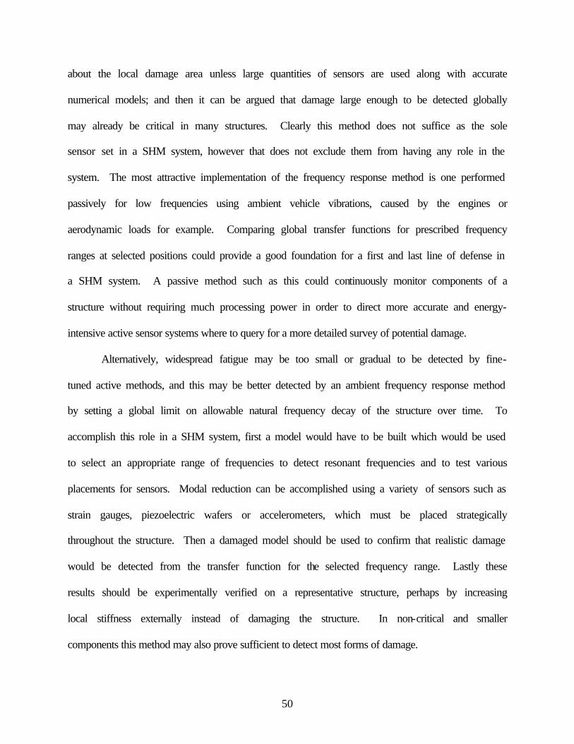
50
about the local damage area unless large quantities of sensors are used along with accurate
numerical models; and then it can be argued that damage large enough to be detected globally
may already be critical in many structures. Clearly this method does not suffice as the sole
sensor set in a SHM system, however that does not exclude them from having any role in the
system. The most attractive implementation of the frequency response method is one performed
passively for low frequencies using ambient vehicle vibrations, caused by the engines or
aerodynamic loads for example. Comparing global transfer functions for prescribed frequency
ranges at selected positions could provide a good foundation for a first and last line of defense in
a SHM system. A passive method such as this could continuously monitor components of a
structure without requiring much processing power in order to direct more accurate and energy-
intensive active sensor systems where to query for a more detailed survey of potential damage.
Alternatively, widespread fatigue may be too small or gradual to be detected by fine-
tuned active methods, and this may be better detected by an ambient frequency response method
by setting a global limit on allowable natural frequency decay of the structure over time. To
accomplish this role in a SHM system, first a model would have to be built which would be used
to select an appropriate range of frequencies to detect resonant frequencies and to test various
placements for sensors. Modal reduction can be accomplished using a variety of sensors such as
strain gauges, piezoelectric wafers or accelerometers, which must be placed strategically
throughout the structure. Then a damaged model should be used to confirm that realistic damage
would be detected from the transfer function for the selected frequency range. Lastly these
results should be experimentally verified on a representative structure, perhaps by increasing
local stiffness externally instead of damaging the structure. In non-critical and smaller
components this method may also prove sufficient to detect most forms of damage.

51
3.6 Conclusions The potential role of the frequency response of a composite structure in a structural health
monitoring system has been investigated in this chapter. A finite element model was built to
explore numerically the effects of various types of damage on the normal modes of test coupons,
and analogous experiments were performed using a scanning laser vibrometer and impedance
meter to verify these results. Good correlation was found between the model and the
experimental results for low frequencies, however coalescing modes at higher frequencies made
comparison impractical. In both the numerical model and experimental results there was strong
correspondence between the extent of damaged (or local stiffness loss) and the reduction in
natural frequency, which again was mostly quantifiable at lower frequencies. This result is
substantiated in several papers in the literature for delamination and notched specimens. The
limitations and sensitivities of the frequency response method are discussed as well. This
method appears to be appropriate for detecting global changes in stiffness, and hence damage, for
relatively large structures at a low power and weight cost. Additionally it has the potential to
deduce this data using only ambient vibration energy in a passive SHM system. A limitation is
that not much information about the specifics of location or type of damage can be inferred by
this method without the use of large stored models. Even so, using ambient vibrations as an
energy source allows the frequency response method to have a potentially useful role in a SHM
system, by guiding other active sensor systems to regions of concern and monitoring the global
decay of structural stiffness.
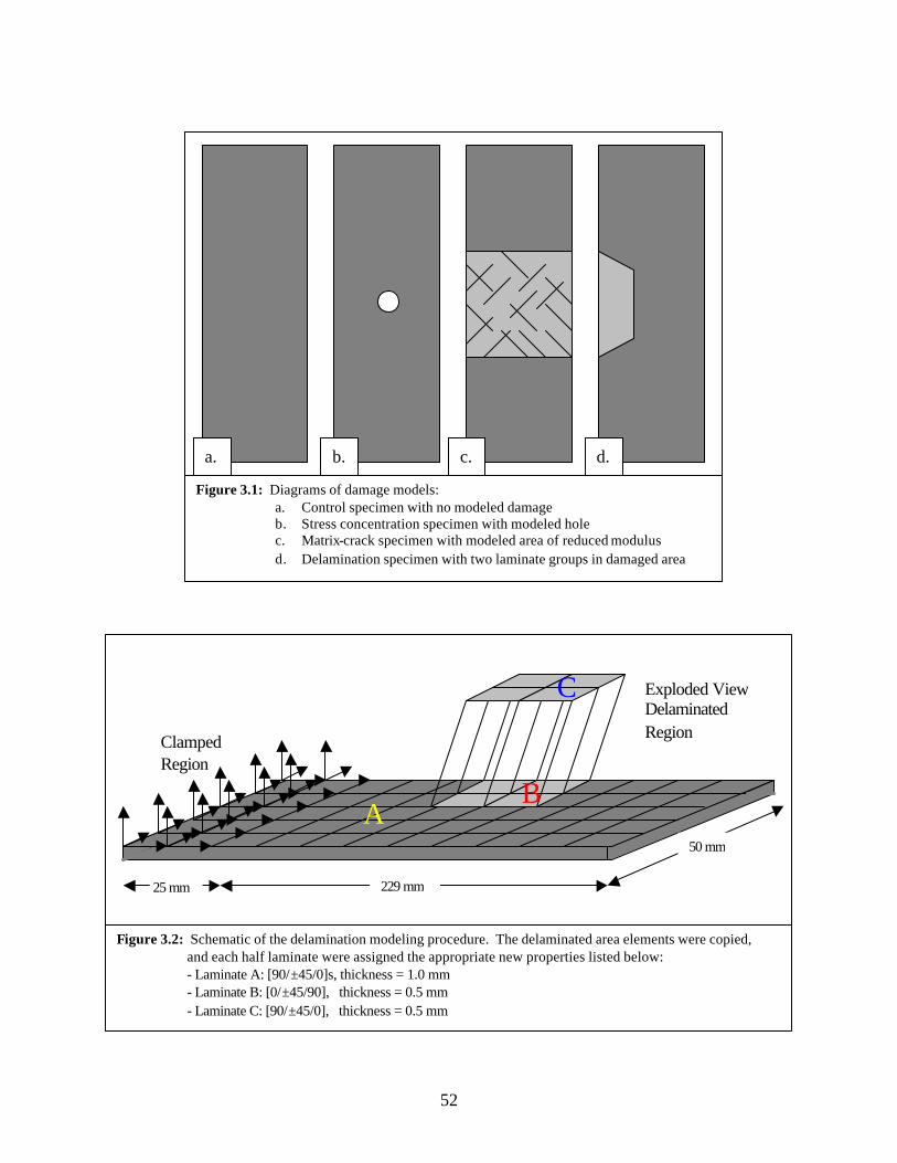
52
Figure 3.1: Diagrams of damage models: a. Control specimen with no modeled damage b. Stress concentration specimen with modeled hole c. Matrix-crack specimen with modeled area of reduced modulus d. Delamination specimen with two laminate groups in damaged area
a. b. c. d.
229 mm 25 mm
50 mm
A B
C
Clamped Region
Exploded View Delaminated Region
Figure 3.2: Schematic of the delamination modeling procedure. The delaminated area elements were copied, and each half laminate were assigned the appropriate new properties listed below:
- Laminate A: [90/±45/0]s, thickness = 1.0 mm - Laminate B: [0/±45/90], thickness = 0.5 mm - Laminate C: [90/±45/0], thickness = 0.5 mm

53
a. b. c. d.
Figure 3.3: X-Radiographs of damaged specimens: a. Control specimen with no damage present b. Stress concentration specimen with drilled through-hole c. Matrix-crack specimen with fatigue induced damage d. Delamination specimen cut with a thin utility knife at the mid-plane
Figure 3.4: Frequency response transfer function plot from FEM in I-DEAS, range 0-20 kHz

54
a. b.
c. d.
Figure 3.5: First four mode shapes of control specimen plotted in I-DEAS. a. first bending, b. second bending, c. first torsion, d. third bending
Figure 3.6: Frequency response transfer function plot from I-DEAS, range of 0-500 Hz

55
Figure 3.7: Frequency response plot from scanning laser vibrometer for range of 0-20 kHz
Figure 3.8: Frequency response plot from impedance meter for full tested range of 0-20 kHz

56
a. b.
c. d.
Figure 3.9: First four mode shapes of control specimen using laser vibrometer data. a. first bending, b. second bending, c. first torsion, d. third bending
Figure 3.10: Frequency response plot from vibrometer for all specimens, range of 0-500 Hz

57
(All Hz) Shape Control Hole Impact Delamination Fatigue Bend Mode 1 1st Bending 12.5 12.4 12.5 12.1 12.1 12.3 Mode 2 2nd Bending 77.8 77.2 77.5 75.5 73.7 76.3 Mode 3 1st Torsion 157 155 156 149 150 154 Mode 4 3rd Bending 218 217 217 211 213 216 Mode 5 4th Bending 428 425 426 412 413 422 Mode 6 2nd Torsion 476 473 474 465 466 472
(All Hz) Shape Control Hole Impact Delamination Fatigue Bend Mode 1 1st Bending 12.5 12.5 12.5 12.5 12.5 12.5 Mode 2 2nd Bending 78.1 78.1 76.5 78.1 75.0 76.3 Mode 3 1st Torsion 157 148 147 137 146 137 Mode 4 3rd Bending 218 217 216 215 209 214 Mode 5 4th Bending 423 423 423 428 413 423 Mode 6 2nd Torsion 461 453 453 451 428 432
(All Hz) Shape 5x2cm Delam
10x2cm Delam
5/4cm Delam
Centered Hole
5cm Offset Hole
-5cm Offset Hole
Mode 1 1st Bending 12.3 12.2 12.2 12.3 12.5 12.2 Mode 2 2nd Bending 76.3 75.6 74.8 77.2 76.9 77.7 Mode 3 3rd Bending 216 213 215 217 216 218 Mode 4 4th Bending 422 418 417 425 426 426 Mode 5 5th Bending 701 691 6931 705 705 706 Mode 6 6th Bending 1050 1030 1040 1060 1050 1060
Table 3.2: Natural frequencies and mode shapes as determined from scanning laser vibrometer data
Table 3.1: Natural frequencies and mode shapes as determined from FEM in I-DEAS
Table 3.3: Natural frequencies and mode shapes from FEM comparing damage in various orientations

58
[This page intentionally left blank]

59
Chapter 4
LAMB WAVE METHODS
This chapter presents analytical and experimental results for the application of Lamb
wave techniques to quasi-isotropic graphite/epoxy specimens featuring representative damage
modes. Linear wave scans were performed on narrow laminated specimens and sandwich beams
with various cores by monitoring the transmitted and reflected waves with piezoelectric sensors.
Similar experiments were also performed on laminated plates and built up composite structures.
Analytical models were built to select optimal actuator configuration and driving signals for
these experiments. Finite element models were also produced for comparison to these
experiments, and to help to predict the detection capabilities of these methods on more complex
structures. Lamb wave techniques have been proven to provide more information about damage
type, severity and location than frequency response methods, and are suitable for structural
health monitoring applications since they travel long distances and can be applied with
conformable piezoelectric actuators and sensors that require little power.
4.1 Background
Several techniques have been researched for detecting damage in composite materials,
however Lamb wave methods have recently re-emerged as a reliable way to locate damage in
these materials [4, 7, 33, 83]. These techniques have been implemented in a variety of fashions
in the literature, including the use of separate actuators and sensors to monitor transmitted waves
60
and/or reflected waves, and multipurpose patches which have both actuation and sensing
capabilities. Each of these techniques offers their own unique advantages in detecting certain
types of damage with various levels of analytical complexity. This section presents the
application of Lamb wave methods as published in the literature.
4.1.1 Early Lamb wave theory and applications
Lamb waves are a form of elastic perturbation that can propagate in a solid plate with free
boundaries [112, 113]. This type of wave phenomenon was first described in theory by Horace
Lamb in 1917, however he never attempted to produce them [114]. Perhaps the earliest
recognition of Lamb waves as a means of damage detection came in 1960 by Worlton of the
General Electric Company [115]. His report investigated the dispersion curves of aluminum and
zirconium to describe analytically the characteristics of the various modes that would pertain to
nondestructive testing applications. The motions and velocities of the interior particles are
formulated, and the effects of holes and thickness variations are discussed. In the following
decade Lamb wave techniques were examined by several investigators, and then the first
potential aerospace application was introduced by Demer and Fentnor of the Hughes Aircraft
Company [116]. In their work they cited ultrasonic wave testing as one of the most reliable
forms of nondestructive testing, and that Lamb waves were emerging as one of the best ways to
infer information about the medium’s density, elastic properties and thickness. They did
however acknowledge the fact that Lamb waves were not readily understood nor easily
interpreted. The particular work performed at Hughes focused on Lamb wave propagation in
metallic thin sheets and elongated cylindrical forms. Fatigue cracks were located in stainless-
steel and aluminum rods by recording the time of flight and attenuated amplitude of the received

61
ultrasonic signal. Similar experiments were performed on glass, ceramic and plastic specimens
with the objective of examining the effects of liquid penetration. In the 1970’s and 80’s, work
on Lamb waves continued and began focusing on various types of actuators. Much of this work
was performed under White at Berkeley, who wrote a comprehensive review paper on all
available forms of actuators and sensors [117]. In it he described mechanical actuation on a line
or using a comb drive, piezoelectric and piezoresistive actuators and sensors operating in d11 or
d13 mode with or without interdigitated electrodes, magnetic or thermal actuators, and optical
sensors. The mechanisms and benefits behind each of these methods are discussed at length, and
follow-up papers were written on the experimental use of the methods which were found to be
the best, which employed silicon-based piezoelectric multisensors [118-120]. Subsequently,
several other authors have written papers that focus on the further development of these
techniques over the past 20 years [121-129].
Since the mid-1990’s, Cawley’s group has had some of the most promising research in
Lamb wave technologies, working to optimize the generation of directional waves [34, 130]. To
allow the implementation of Lamb waves on a real structure, they have been developing flexible,
cheap Polyvinylidenedifloride (PVDF) transducers in order to both generate and detect waves.
Their work uses interdigital transducer leads to generate highly focused and directional waves
without higher mode interference, and they have inspected various metallic specimens with
encouraging results. During more recent work, Cawley’s group has been experimentally testing
the limitations of their methods on large areas and thick structures representing sections of
aircraft fuselages [131, 132].
62
4.1.2 Lamb waves in composite materials
During the late 1980’s and early 1990’s work began on the application of Lamb waves to
composite materials. Research conducted at NASA by Saravanos demonstrated, both
analytically and experimentally, the possibility of detecting delamination in composite beams
using Lamb waves [133, 134]. Similar conclusions were drawn by Percival and Birt at the
Defense & Evaluation Research Agency, UK, who began focusing their work on the two
fundamental Lamb wave modes, which will be described further in the following section [135-
137]. Detection of other forms of damage in composite materials was also investigated by Seale,
who examined fatigue and thermal damage, and Tang who observed the sensitivity of Lamb
wave propagation to fiber fracture [138, 139]. This work was extended to composite sandwich
plates, including panels subjected to impact damage by Osmont and Rose [80, 140]. There have
also been several others recently who have begun to investigate the interaction of Lamb waves
with composite materials [64, 141-144].
The most successful work to date using Lamb waves for damage detection in composite
materials has been performed by Soutis’s group at Imperial College, who have focused on the
sensor placement and signal processing issues [81, 82, 144]. They have chosen to use Lead-
Zirconate-Titanate (PZT) actuators and sensors over PVDF since they require a factor of ten less
voltage to generate Lamb waves, however they are not as conformable. The most complete work
from this group can be found in Valdez’s PhD thesis [96]. During the course of his work he
performed many experiments on quasi-isotropic graphite/epoxy composite specimens, pulsing
them with Lamb waves in various configurations to detect controlled artificial delaminations. He
also simulated the propagation of Lamb waves in plates of various widths using a finite element
code. Much of the Lamb wave research presented in this thesis follows Valdez’s work,

63
extending it to various other types of damage, and furthermore testing sandwich structures and
built-up structures as well as addressing self-sensing actuators and analytically optimizing the
experimental procedures.
4.2 Analytical Procedures
There are two groups of Lamb waves, symmetric and anti-symmetric, that satisfy the
wave equation and boundary conditions for this problem, and each can propagate independently
of the other. A graphical representation of these two groups of waves can be seen in Figure 4.1.
The present work utilizes PZT piezoelectric patches to excite the first anti-symmetric Lamb
wave (A0 mode). This wave was chosen since it can propagate long distances with little
dispersion, and no higher modes are present to clutter the resulting response waves [96]. In the
following section, analytical models for Lamb wave propagation have been derived, which relate
the velocity of the wave-front to the actuating frequency. Using these equations along with other
mathematical principles found in the literature, limitations of Lamb wave propagation have also
been defined. Lastly, finite element models were built to simulate the travel of these waves in
each of the test setups to help specify setup parameters and predict experimental results.
4.2.1 Dispersion curve formulation
The most descriptive way to represent the propagation of a Lamb wave in a particular
material is with their dispersion curves, which plot the phase and group velocities versus the
excitation frequency [112]. The derivation of these curves begins with the solution to the wave
equation for the anti-symmetric Lamb wave as seen in Equation 4.1:
0
--14
)12(
)-dtan(
)-1dtan(2222
22
22
2
=−
+ζξζζ
ζ
ζξ
ζ(4.1)

64
where the non-dimensional parameters are: For an isotropic material, these parameters can be defined in terms of Lamé’s constants: In which case: Substituting these equalities into the non-dimensional parameters yields:
Finally, Equation 4.5 was substituted into Equation 4.1 to be solved numerically in
Mathematica , as described in Appendix A. For a given material, the Young’s Module in the
propagation direction E, Poisson Ratio v, and the density ρ are known, and the phase velocity
cphase is the dependent variable being solved for. The independent variable being iteratatively
supplied is the frequency-thickness product, where ω is the driving frequency in radians. An
example of a phase velocity dispersion curve for the first anti-symmetric Lamb wave using the
material properties from the specimens used in the present research can be seen in Figure 4.2.
The other useful plot is the group velocity dispersion curve, which can easily be derived from the
phase velocity curve using Equation 4.6:
2
kd , , t
2
22
2
22 t
cc
cc
phase
t
l
t === ζξ
))(12-(1E
, )2(1
Eνν
νλ
νµ
+=
+=
tlt c
ccω
ρµλ
ρµ
=+
== t22 k ,
)2( ,
E)1(2
222d
)1(2E
, 2221
)2( 2222
νρωµρωω
νρρµ
ζνν
µλµ
ξ
+===
+==
−−
=+
=
ttct
cc
t
phasephase
fc
cfc
kk
ccc
f
cK
phase
phase
phasephasephasegroup
phasew
w
∂∂
⋅−=
∂∂
+=
==
1
)wavelength( r),(wavenumbe 2
λλπ
(4.2)
(4.3)
(4.5)
(4.6)
(4.4)

65
where f is the frequency in Hz. An example of a group velocity dispersion curve, again using the
material properties from the present research can be seen in Figure 4.3. At low frequencies, the
Ao phase velocity can be approximated in the form of Aω½ and the complementing group
velocity as 2Aω½, where A is a material property dependant constant. At higher frequencies the
phase velocity for this mode tends to the Rayleigh velocity:
A more thorough derivation of these velocities, starting from Lamb’s equalities can be found in
Appendix B. These dispersion curves are the key to describing and understanding the
propagation of Lamb waves in a solid medium, and will be used in the following sections to
predict the effects of damage in a given structure.
4.2.2 Propagation and limitations of Lamb waves
The relationship between the material properties of a specimen and the velocity of the
propagating Lamb wave is quite complex, however an understanding is necessary to design an
appropriate damage detection method. By inspection of Equation 4.1, to first order the wave
velocity increases with the square root of the modulus, i.e. an increase in modulus slightly speeds
the wave velocity. An increase in the density would have the opposite effect slowing wave
velocity, as it appears in all the same terms as the modulus but on the reciprocal side of the
divisor. The effect of the Poisson’s ratio is probably the most complicated, as it appears in most
of the terms, and small changes seem to have little to no effect on the wave velocity. The most
straightforward parameter is the thickness of the specimen, which has a linear relationship with
the Lamb wave velocity—the thicker the specimen the quicker the wavespeed.
tR cc
++
=ν
ν1
12.187.0 (4.7)
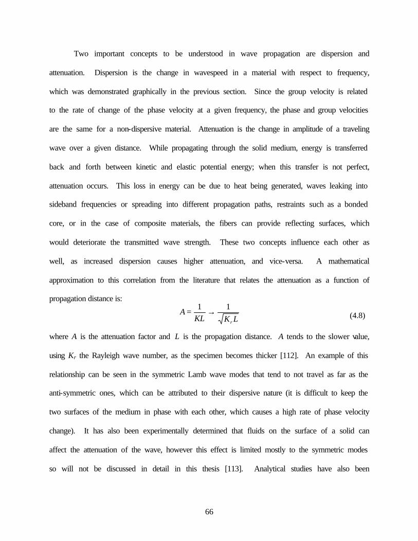
66
Two important concepts to be understood in wave propagation are dispersion and
attenuation. Dispersion is the change in wavespeed in a material with respect to frequency,
which was demonstrated graphically in the previous section. Since the group velocity is related
to the rate of change of the phase velocity at a given frequency, the phase and group velocities
are the same for a non-dispersive material. Attenuation is the change in amplitude of a traveling
wave over a given distance. While propagating through the solid medium, energy is transferred
back and forth between kinetic and elastic potential energy; when this transfer is not perfect,
attenuation occurs. This loss in energy can be due to heat being generated, waves leaking into
sideband frequencies or spreading into different propagation paths, restraints such as a bonded
core, or in the case of composite materials, the fibers can provide reflecting surfaces, which
would deteriorate the transmitted wave strength. These two concepts influence each other as
well, as increased dispersion causes higher attenuation, and vice-versa. A mathematical
approximation to this correlation from the literature that relates the attenuation as a function of
propagation distance is:
where A is the attenuation factor and L is the propagation distance. A tends to the slower value,
using Kr the Rayleigh wave number, as the specimen becomes thicker [112]. An example of this
relationship can be seen in the symmetric Lamb wave modes that tend to not travel as far as the
anti-symmetric ones, which can be attributed to their dispersive nature (it is difficult to keep the
two surfaces of the medium in phase with each other, which causes a high rate of phase velocity
change). It has also been experimentally determined that fluids on the surface of a solid can
affect the attenuation of the wave, however this effect is limited mostly to the symmetric modes
so will not be discussed in detail in this thesis [113]. Analytical studies have also been
LKKLA
r
11 →= (4.8)
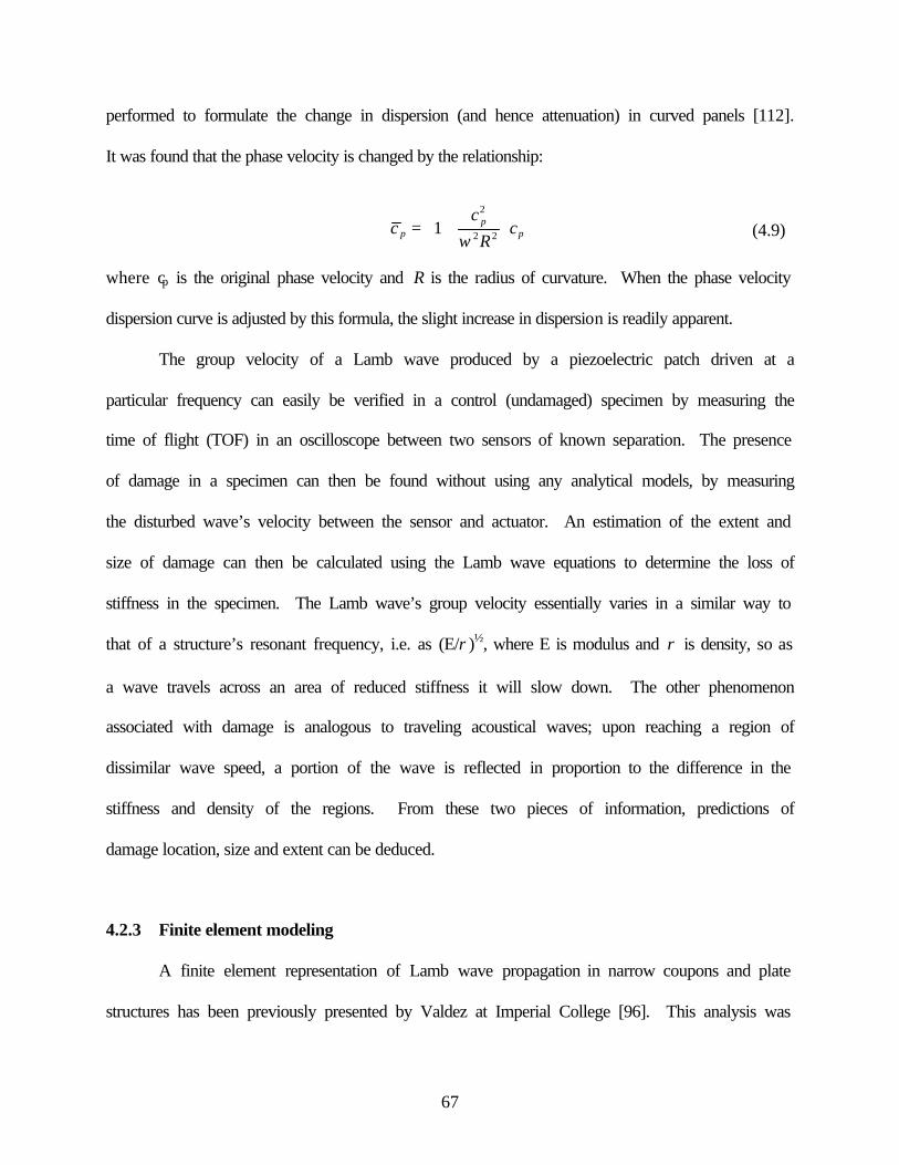
67
performed to formulate the change in dispersion (and hence attenuation) in curved panels [112].
It was found that the phase velocity is changed by the relationship:
where cp is the original phase velocity and R is the radius of curvature. When the phase velocity
dispersion curve is adjusted by this formula, the slight increase in dispersion is readily apparent.
The group velocity of a Lamb wave produced by a piezoelectric patch driven at a
particular frequency can easily be verified in a control (undamaged) specimen by measuring the
time of flight (TOF) in an oscilloscope between two sensors of known separation. The presence
of damage in a specimen can then be found without using any analytical models, by measuring
the disturbed wave’s velocity between the sensor and actuator. An estimation of the extent and
size of damage can then be calculated using the Lamb wave equations to determine the loss of
stiffness in the specimen. The Lamb wave’s group velocity essentially varies in a similar way to
that of a structure’s resonant frequency, i.e. as (E/ρ)½, where E is modulus and ρ is density, so as
a wave travels across an area of reduced stiffness it will slow down. The other phenomenon
associated with damage is analogous to traveling acoustical waves; upon reaching a region of
dissimilar wave speed, a portion of the wave is reflected in proportion to the difference in the
stiffness and density of the regions. From these two pieces of information, predictions of
damage location, size and extent can be deduced.
4.2.3 Finite element modeling
A finite element representation of Lamb wave propagation in narrow coupons and plate
structures has been previously presented by Valdez at Imperial College [96]. This analysis was
pp
p cR
cc
+= 22
2
1ω
(4.9)

68
reproduced in the present research by ABAQUS models to observe the small changes in time
of flight caused by discontinuities in geometry or material properties. Models were built to
represent each of the experiments that were performed, including narrow coupons, sandwich
beams, 2-D plates with and without stiffening ribs, and finally a tube structure with sandwich
construction. Each of these models were constructed identically to those described in the
previous frequency response methods chapter, using 1 cm2 square shell elements, where the
actuators were simulated by a coupled nodal moment. Again regions of cracked matrix were
modeled as a local loss in stiffness, and delaminations were modeled by two half laminates with
coincident unconnected nodes. Representative input files for these models can be found in
Appendix C. Once processed, the time-steps were visualized as a movie file to measure the time
of flight of the Lamb waves across the specimens, and to record visual evidence of dispersion
and attenuation. By comparing the times of flight in these models, it was possible to determine
the required distance between the piezoceramic actuator and sensors necessary to resolve the
difference between waves traveling in a control versus a damaged specimen.
A different approach was taken by Prosper at MIT, who produced a thin layered
laminated medium finite element code to solve for the propagation of elastic waves in a two-
dimensional through-thickness cross-section [145]. This code was modified by Prosper for the
present research to incorporate the graphite/epoxy material properties, thickness and driving
signal used in the experimental procedure to observe the progression of Lamb waves. Models
were created for both control and delaminated specimen, by leaving a section of layered nodes
unconnected. The results of the finite element simulations were animations to observe the
motion of the deflected surface material with respect to time to be compared with the more
traditional two-dimensional surface finite element models from ABAQUS.

69
4.3 Optimization Procedures There is currently no standard or even a best-practice precedent for damage detection via
Lamb wave testing. Several procedures have been developed in the literature, each with valuable
characteristics, and each with some degree of arbitrariness. A major goal of the present research
was to optimize, analytically and experimentally, the Lamb wave testing procedure, and to
determine what effects various parameters have on the sensitivity of damage detection. These
parameters can be divided into three categories: actuating frequency, pulse shape, and sensor
geometry. The following sections provide selection guidelines for each of these categories,
which were used to define the testing parameters for the experimental procedures that followed.
This set of tools could be used in parallel by an engineer developing a SHM system for a vehicle
to decide if the Lamb wave method would provide satisfying results for their application, and to
determine the appropriate driving parameters to obtain the best damage detection resolution.
4.3.1 Frequency selection
The first step in defining an appropriate Lamb wave damage detection solution is to
select an appropriate driving frequency, as demonstrated in the flowchart in Figure 4.4. This
procedure commences by finding the Lamb solution for the wave equation, and plotting the
dispersion curves for each section to be monitored. The equations presented previously in this
chapter are intended for isotropic materials, however it has been shown in the literature that the
Ao mode is fairly invariant to the layup of a composite material, and can be closely approximated
by using the bulk laminate properties [136]. Finite element techniques have been used by other
researchers in the literature to more accurately determine the wave velocities in composite
materials [135, 138]. By entering the material properties (E, ν, and ρ) for a particular material,

70
the resulting dispersion curves provide a range of potential wave velocities for the A0 mode
driven at different frequency-thickness products. For a given thickness, ideally one would like to
choose the least dispersive driving frequency for the Lamb wave being generated, which
generally exists where the slope of the phase velocity curve is equal to zero. This is because at
low frequencies, the dispersion curves have steep slopes and thus are very sensitive to small
variations in frequency making it difficult to maintain a constant velocity to predict the time of
flight. The A0 mode, however, follows a square root relationship until higher frequencies, thus
the frequency needs to be chosen by a different criteria. The higher the frequency the smaller the
slope of the A0 dispersion curve, although at a certain point other higher order Lamb waves begin
to exist simultaneously and the signal becomes cluttered. The wave velocities are also much
quicker at higher frequencies, increasing the requirements for data acquisition.
To balance these issues, the following procedure should be followed. First plot the
dispersion curves for the material, and locate the frequencies at which the Rayleigh velocity is
obtained and where the A1 mode begins to be excited. If the Rayleigh velocity is below the point
where the next anti-symmetric mode is generated (which normally is not true) then this is the
critical frequency; otherwise it would be wise to choose a point about 10% below the A1 origin
point as the critical frequency. Next, it must be determined if the data acquisition capabilities are
able to capture a wave traveling at this velocity. Typically, the data acquisition rate should be 10
times the frequency of the signal it is sampling, so the selected driving frequency may have to be
lowered if the sampling rate is unobtainable. Also, with knowledge of the effects of various
damage types on the stiffness of a particular material, the resolution of change for the resultant
signal, or “observeability,” can be predicted in order to determine the detection limitations with
respect to flaw size for a given data acquisition capability. It would also be prudent to check on

71
the actuator capabilities to generate that range of frequencies. A final consideration to fine tune
the driving frequency is to calculate the natural frequencies of the structure to be monitored,
either analytically or by finite element models, and to select a driving frequency that coincides
with a normal mode in the desired frequency range. The natural frequencies of the structure play
a small role in the amplification or attenuation of the transmitted wave, whereas the wave can
travel with less disturbance at a resonant frequency.
Using this approach, an effective experimental test procedure was determined for the
present research. The material constants in the propagation direction for the composite laminates
to be analyzed were calculated by classical laminated plate theory, and then entered into the
Lamb wave model. For the narrow coupon tests, 15 kHz was selected as an optimal frequency,
50 kHz for the sandwich beam tests, and 40 kHz for the micro-satellite bus structure (all to be
described further in the experimental procedures section). These frequencies were obtained from
their slope and location on the dispersion curves, evidence from previous research suggesting
these frequencies for specimen of similar geometries, and brief experimentation using a function
generator to verify the maximum response amplitude for the range of driving frequencies.
Following this procedure it was determined that graphite/epoxy composite materials were a good
candidate for Lamb wave methods, and that with the detection capabilities of the data acquisition
system that a reasonable change in stiffness (5-10%) could be resolved.
4.3.2 Pulse shape selection
The second set of variables explored was the actuation pulse parameters. These included
the pulse shape, amplitude and number of cycles to be sent during each pulse period. These
parameters were varied analytically and verified experimentally on a control specimen to observe

72
their effect on the Lamb waves generated. First, several candidate signal shapes were compared
in Matlab by using their power-spectral-density (PSD) plots. Similarly the effect of the
number of cycles per period for the different shaped signals was observed in the PSD plots by
comparing the energy dedicated to the principal driving frequency. The more energy dedicated
to the desired driving frequency, the stronger the Lamb wave and the more accurate the
wavespeed calculation, and hence the more sensitive and reliable the damage detection
capability. Of the signal shapes that were analyzed and experimented, pure sinusoidal shapes
appear to excite Lamb wave harmonics the most efficiently, since they are periodic, smooth and
have comparatively quick rise times to their peak amplitude as compared to a parabolic shape. A
Hanning window (approximated by a half-sine wave multiplied over the pulse width) helps to
narrow the bandwidth further to focus the maximum amount of energy into the desired actuating
frequency with the least “spill-over” from neighboring frequencies.
Once the driving frequency and signal shape have been selected, there is then a trade
between the number of waves that can be sent in an actuating pulse and the distance from abrupt
features in the structure. The number of cycles of a periodic function desired to actuate the
piezoelectric actuator is one of the more complicated decisions to be made for Lamb wave
techniques. The fast Fourier transform (FFT) of a continuous sine wave would yield a single
peak at the driving frequency, however for a few finite cycles, the FFT appears as a Gaussian
curve with a peak at the driving frequency. Thus, the more waves sent into a driving pulse, the
narrower the bandwidth and the less dispersion. The problem in a short specimens though, or in
applications where the actuator and sensors are spaced close together, is the more waves in the
pulse the less time between the last signal sent and the first returning reflected signal, so the
response is more difficult to interpret. An appropriate number of cycles can be determined by
73
the maximum number of waves that can be sent in the time it takes for the lead wave to travel to
the sensing PZT patch. It is also convenient to use intervals of half cycles so that the sent
sinusoidal pulse becomes symmetric. Research from the literature has used signals varying from
3.5 to 13.5 cycles per actuating pulse [34, 80-82, 96, 144]. Since the specimens in the current
research are relatively short, few cycles could be actuated without disturbing the received signal
thus 3.5 cycles were used to drive the piezoceramic actuators.
Lastly, by increasing the driving voltage the magnitude of the strain produced by the
propagating Lamb wave proportionately increases. In these experiments, driving the
piezopatches at an amplitude of 5-10V produced a 10-25 mV response due to the wave sensed by
the PZT patch. Increasing the amplitude also increases the signal-to-noise ratio to yield a clearer
signal, since the static noise received by the PZT patch is usually in the 1-5 mV range. Higher
voltage however also tended to increase the drift in the signal, which deteriorated the resolution
capabilities of the data acquisition system. Also, a SHM system should be as low power as
possible, thus the voltage should be chosen to be the minimum required to resolve the desired
damage size. The driving voltage was chosen to be 10V peak-to-peak for these experiments.
4.3.3 Actuator selection
PZT 5H piezoceramic actuators were chosen for the present research due to their high
force output at relatively low voltages, and their good response qualities at both low and high
frequencies. The shape of the actuator should be chosen based upon desired propagation or
reception directions. Researchers in various fields have examined the effects of piezoelectric
wafer dimensions on the efficiency of their actuation [146, 147]. Waves propagated parallel to
each edge of the actuator, i.e. longitudinally and transversely for a rectangular patch and

74
circumferentially from a circular actuator. The width of the actuator in the propagation direction
is not critical, however the wider it is, the more uniform the waveform created. As cited in the
literature though, there is an important sinusoidal relationship between actuating frequency and
actuator length [112]. In the direction of propagation the desired actuator length 2a is:
This value of 2a could either be a rectangular side length or the diameter of a circular actuator.
This equation could also be used to determine actuator minimum dimensions, in order to inhibit
waves from propagating in undesired directions. For the experimental procedures in the present
research, PZT actuators of 1.5 cm x 0.75 cm were selected based upon this equation.
The other critical issue with actuator selection is the determination of spacing between
the actuators and sensors. A design objective of a SHM system is to achieve the most structural
coverage with the least number of sensors, thus the optimal sensor spacing must be calculated.
The governing equation to estimate this spacing is the attenuation equation presented in a
previous section (Equation 4.8), which specified an inversely proportional relationship between
propagation distance and signal amplitude that was also dependant on the wave number. An
acceptable signal loss can be specified for the voltage sensitivity of a data acquisition system,
which was determined to be 25% for the present experiments, and from this percentage an
estimated actuator-sensor spacing can be calculated.
4.3.4 Signal interpretation
The key to reliable and high-resolution damage detection is good signal interpretation.
The raw signals taken from the sensors are in the form of a time history of small voltages caused
3... 2, 1, 0, nfor 21
21
2 =
+=
+= n
f
cna pλ (4.10)

75
by strains induced by the impinging Lamb waves. The first problem with this recorded signal is
noise. The largest source of error in the present research was parasitic capacitance in the data
acquisition system. In order to acquire data at high frequencies through several channels most
data acquisition systems use multiplexers, or MUX. These devices scan through each channel
one at a time, making an electrical connection to charge a capacitor from which the voltage
measurement is taken, and then moving on to the next channel. The principal limitation on this
approach is the occurrence of parasitic capacitance when the data acquisition rate is higher than
the settling time of the system, so that residual charge is left on the capacitor in the MUX as it
moves from one channel to the next. This effect was further enhanced in the present research
since the triggering channel was measuring the driving signal voltage at a range of ±5 V and the
other channels were using a range of ±50 mV to measure the sensor voltages. This resulted in a
large “ghosting” effect across all the channels, where the driving signal could be seen at a
slightly reduced voltage in each of the other measurements. Since the high rate of data sampling
was necessary to record the impinging waves, the solution adopted was to use an attenuator to
reduce the amplitude of the driving signal being measured in the data acquisition system, while
not affecting the driving voltage being split off to the actuator. All of the other systematic
sources of noise, which included strains caused from external sources such as air currents and
vibrations in the building, were accounted for by connecting an unattached sensor to a blank
channel, and using it to normalize the signals from the other channels.
Perhaps the most important factor that has allowed Lamb wave techniques to flourish
recently is the development of wavelet analysis. Wavelet decomposition is similar to the Fourier
decomposition, however instead of just using sines and cosines, complex “mother wavelets” are
used to break down the signal [148]. The idea for the wavelet decomposition was first presented

76
by Haar in 1910, however the square wave he used was not very practical for most applications.
It was not until 1988 when Daubechies introduced a fractal-like mother wavelet, that the full
potential of wavelet analysis for signal decomposition and compression realized. The mother
wavelet is essentially used as an orthogonal basis vector to filter the signal, and is scaled and
shifted to approximate the frequency components of the signal. Typically this decomposition is
not done continuously since most of the mother wavelets have no closed form solutions. As
result a discrete transform on buffered portions of a signal is typically used. This can be
performed in commercial software packages such as MATLAB using codes such as that
presented in Appendix D.
The present research used the Morlet wavelet to decompose the signals, since its shape
was closest to the driving pulse shape, which makes the processing more accurate and efficient
[34]. To analyze the measurements, the Morlet wavelet was scaled between 0 Hz and twice the
driving frequency and it was subsequently shifted through the entire time axis. The results of
this analysis could be visualized in two forms. The first was a waterfall plot, which plots all the
frequency scales versus time, representing the energy present at a point by color-coded intensity.
Secondly, each of these scale bands could be plotted independently to allow observation of the
numerical amplitude of signal energy versus time. Using the second method, by looking at the
central scale band one could filter out all frequencies other than the central driving frequency
from the received signals. This provides a clear, filtered view of the transmitted energy from the
actuator to the sensors over time for an accurate time of flight measurement. Then, by looking at
the waterfall plot, one could potentially gain insight into the damage in the specimen from the
intensities of energy that have been shed into sideband frequencies. The experimental results
presented later in this chapter were created using this procedure.

77
4.4 Experimental Procedures
This section describes the experimental procedures that were followed during the course
of the present research to validate the effectiveness of Lamb wave methods as a means of
damage detection in composite materials. These experiments followed a building block
approach [149], commencing with the reinvestigation of the narrow coupon specimens used
during the frequency response tests, then investigating laminated plates and finally built-up
structures. Core-filled sandwich panel structures were also tested. All of these tests used PZT
piezoceramics as both actuators and sensor in pulse-transmission mode. Separate experiments
were performed to evaluate a method that used “self-sensing” PZT actuators.
4.4.1 Narrow coupon tests The first set of experiments was conducted on narrow composite coupons. The laminates
used for this present research, both for control specimens and those with simulated damage, were
manufactured during previous tests that explored frequency response methods as a means of
damage detection, and were re-used to compare directly the effectiveness of the two methods
[150]. The specimens were 25 x 5 cm rectangular [90/±45/0]s quasi-isotropic laminates of the
AS4/3501-6 graphite/epoxy system, which were clamped on one end to match the boundary
conditions from the previous research (however experimentation proved that the boundary
conditions around the frame of the specimen had no effect on the Lamb wave traveling between
two piezoceramic patches). Three PZT piezoceramic patches were affixed to each specimen, as
shown in Figure 4.5, using 3M ThermoBond thermoplastic tape so that they were firmly
attached during testing, but could be removed afterwards to recover the specimens for future
tests. The PZT was cut into 2 x 0.5 cm patches so that the longitudinal wave would be favored
78
over the transverse one, and three patches were used on each specimen to actuate and to measure
the transmitted and reflected waves. Both the actuation and the data acquisition were performed
using a portable NI-Daqpad 6070E data acquisition board, and a laptop running Labview as
a virtual controller. A Labview VI-file, seen in Appendix E, was created which would load an
arbitrary waveform from Matlab and output it at the desired frequency and amplitude, while
simultaneously acquiring data on four channels at 600,000 samples per second. The output
channel was connected directly to the actuating PZT, generating the desired waveform with an
amplitude of 10V. The first input channel, which served as the trigger for all of the channels,
was connected to the output channel through an attenuator to scale the amplitude down by two
orders of magnitude, two others were connected to the sensing piezoceramic patches, and the
final channel was connected to a PZT sensor not attached to the specimen to serve as a control
channel in order to zero out drift. A single pulse of the optimal signal found in the previous
section, shown in Figure 4.6, was sent to the driving PZT patch to stimulate an A0 mode Lamb
wave, and concurrently the strain-induced voltage outputs of the other two patches were recorded
for 1 ms to monitor the wave propagation.
The data was then passed to Matlab where the drift was filtered out and the waveforms
could be compared and analyzed within two specialized toolboxes. In the signal processing
toolbox the waves could be superimposed, and a peak detector was used to determine accurately
the time of flight for each signal, and the delay in time of arrival between two specimens.
Subsequently, in the wavelet toolbox a Morlet wavelet was used to perform a time-frequency
decomposition of the data. By plotting the magnitude of the wavelet coefficient at the peak
driving frequency, the energy remaining from the input signal could be compared [151]. This
procedure was carried out for three of each specimen types at a driving frequency of 15 kHz.

79
4.4.2 Sandwich beam tests
Analogous experiments were performed on sandwich coupons to that of the narrow
laminates in order to test the effect of various types of core materials on the propagation of Lamb
waves. Four different cores were used: low and high density (referred to as LD and HD)
aluminum honeycomb, Nomex, and Rohacell, all seen in Figure 4.7. Each specimen
contained two facesheets identical to the undamaged laminates in the previous section
surrounding a 2 cm thick core, which were adhered using FM-123 film adhesive in a secondary
curing process [110]. Two controls and two damaged specimens of each type were
manufactured for testing. In the damaged specimens, a 5 x 2.5 cm piece of Teflon was placed
between the adhesive and the core in a central 2.5 cm region during the cure so that the facesheet
would not bond to the honeycomb to simulate a delamination. An additional specimen was also
manufactured with the high density aluminum core that had a 2 cm diameter circular piece of
Teflon placed between the layers on either side so that it was indistinguishable from the controls
by sight. This specimen was used for a “blind test” of the proposed Lamb wave damage
detection method, where it was tested alongside the two control specimens to determine which
had the artificial flaw. The test setup and data analysis procedure for the sandwich beam
experiments were identical to that of the thin specimens with the exception of the driving
frequency, which was determined to be more effective at 50 kHz for these tests.
4.4.3 Stiffened plate tests
The next set of experiments examined damage detection in more complex stiffened
specimens using Lamb waves. Laminated plates were manufactured similarly to the ones from
the previous sections, however these specimens included a secondary cure in which ribs were

80
bonded across the center of the plate using Cytec FM-123 film adhesive. Three different
configurations of ribs were tested during this section of research, as seen in Figure 4.8. The first
had a thin 2.5 cm wide aluminum C-channel rib with 1.2 cm tall webs, which was adhered to the
laminate with the flat side facing down and the channel parallel to the sensors. The second
configuration used two scrap pieces of the same composite laminate, one 2.5 cm wide and the
other 1.2 cm wide, which were bonded with FM-123 in a pyramid-like stack in the center of the
laminate, again parallel to the sensors [110]. The final configuration was identical to the second
one, except it had a 2.5 cm square Teflon strip inserted between the stiffening rib and the
composite to create an artificial delamination in the center of the rib. For each of the
configurations, actuating and sensing PZT sensors were affixed to opposite sides of the rib on the
edges of the laminate in three locations—one pair that was centered on the laminate and one pair
on either side of the centerline spaced 7.5 cm away. The purpose of these experiments was first
to examine how the rib would effect the propagation of the Lamb waves, then to compare the
propagation through ribs of various stiffness, and lastly to ascertain the feasibility of locating a
delaminated region under a rib by comparing the received signal with undamaged regions. The
test setup and data analysis procedure for the stiffened panel experiments were identical to that
of the thin specimens with a driving frequency of 15 kHz.
4.4.4 Composite sandwich cylinder tests
The next level of complexity involved examining a relatively large built-up structure, a
cylinder with a 40 cm diameter and length of 120 cm, seen in Figure 4.9, which was constructed
during previous research as a composite micro-satellite structure [152]. The two facesheets of
the sandwich structure were manufactured from the same composite material as the other tested

81
specimens and were of similar layup, and a 2.5 cm thick low-density aluminum honeycomb was
bonded between them. An identical setup to that used on the other specimens was used on this
cylinder to determine the feasibility of detecting known damaged regions in a large curved built-
up structure. First, in a control region with no visual damage, an actuating PZT wafer was
placed on one end of the cylinder, and then sensing piezoceramic patches were placed down the
length of the cylinder every 10 cm for 60 cm. These tests would not only provide a controlled
time of flight for the structure, but would also provide data for the attenuation of the wave in a
representative structure. Next sensors were placed every 10 cm circumferentially over a 30 cm
span to examine the attenuation of the Lamb wave signal in a curved section. Lastly,
piezoelectric sensors were adhered in positions 10 cm away longitudinally and at 5 cm
increments circumferentially to attempt to quantify how far away from the main propagation
channel the sensors could be placed to still sense a reliable measurement. Once again, the data
analysis procedure for these experiments were identical to that of all the others, with a driving
frequency of 40 kHz in this case because of the honeycomb core and slightly different layup.
4.4.5 2-D plate tests
The final test performed in pulse-transmission mode was to scan 2-D laminated plates for
damage. Graphite/epoxy panels measuring 30 x 30 cm were manufactured similarly to those of
the previous experiments, but were not milled into smaller specimen for these experiments.
Square PZT sensors measuring 1.5 cm on each side were affixed along the perimeter of the
laminate, in the center of each side as seen in Figure 4.10. The driving pulse was sent to actuate
each PZT piece one at a time at 15 kHz, and simultaneously readings of resulting strains were
82
measured from each of the other three patches; this would occur four times, each time actuating a
different piezoelectric sensor. These results were also decomposed using the Morlet wavelet.
4.4.6 Self-sensing tests
As an alternative to pulse-transmission, some preliminary testing was also performed for
the pulse-reflection of Lamb waves. Theoretically, this method should provide more information
about damage location, since the time of flight of damage from reflection sites would be
recorded so a triangulation could be performed. The setup for these tests was identical to the
configuration from the 2-D plate tests, with PZT sensors placed in the center of each side. The
only difference for these tests was that each PZT piece would serve as both a sensor and receiver
simultaneously, collecting the reflected as well as the transmitted strain data for each pulse
actuation. This “self-sensing” capability was achieved by using a full bridge circuit, represented
in Figure 4.11, which was developed in the literature and adapted for use in these experiments.
This circuit design would allow the data acquisition equipment to monitor the 10 mV strain
measurements from the PZT without being overwhelmed by the 5 V driving signal [153].
4.5 Results
This section presents the results for analytical and experimental procedures previously
described in this chapter. The analytical results are in the form of time of flight measurements
taken from the movie files created by the finite element solution in ABAQUS. Several
snapshots of the propagating waves are also displayed. The experimental results summarize the
comparison of the wavelet-decomposed signal between the control specimen and the specimens
with various forms of damage. The presence of damage in the specimens caused the amplitude

83
of the wave coefficients to decrease significantly, as well as slowing the wave velocity for many
of the specimens. These results are presented for narrow coupons, sandwich beams, stiffened
panels, a composite sandwich cylinder and a 2-D laminated plate. A discussion of these results
is presented in the following section.
4.5.1 Analytical results The first set of analytical results were obtained from the thin layered laminated medium
finite element code written by Prosper at MIT as described previously, which accurately
characterized the cross-sectional variation due to the Lamb wave, however was incapable of
analyzing changes in the width direction. A representative plot showing the vertical
displacement over time at a point 25 cm away from the 60 kHz actuation point can be seen in
Figure 4.12. The solid line in this figure represents the undamaged graphite/epoxy specimen
that appears to have a wave velocity of around 1.95 km/s, while the broken line is a simulation of
the Lamb wave traveling at 1.85 km/s in a specimen with a 2.5 cm center delamination. There
also appears to be a slight change in wave frequency content for the Lamb wave in the
delaminated specimen.
The next set of results were obtained from the finite element models created in
ABAQUS, which simulated the behavior of the Lamb waves as they traveled across the thin-
shelled laminate. The products of these analyses were movie files that animated the vertical
displacement of the nodes over time as the Lamb waves propagated from the loaded nodes. A
series of still shots of a Lamb wave propagating in a control model can be seen in Figure 4.13
and for a delaminated model in Figure 4.14. A summary comparing the recorded times of flight
for each of the models that were analyzed can be found in Table 4.1. The FE results did not
84
show much of a change between the control and cracked models for time of flight, however there
was a noticeable reflected wave traveling from the cracked region after the Lamb wave had
passed over it. The model with the through-hole exhibited a slight change in time of flight, and a
small reflected wave was observed as well. For both delamination models there was a significant
increase in the time of flight due to the damage, and in addition, reflected waves were generated
which had almost half the amplitude of the traveling wave. Additionally, the model with the
asymmetric delamination created two wave fronts traveling at different speeds, which began to
interfere with each other as they continued down the laminate. These FE results appear to be
consistent with the experimental results, as will be further discussed in the following section.
Comparable results were found for each of the sandwich beam models, control and
stiffened plate models and curved sandwich panel models. The time of flight measured for each
of these models is documented in Table 4.2. Perhaps the most interesting results were
discovered for the stiffened plate models. First, Figure 4.15 displays the Lamb wave as it
propagated across a plate with no stiffener attached as a controlled reference. Next, as seen in
the series of stills for the plate with bonded composite stiffeners in Figure 4.16, as the wave
traveled radially from the actuation region and reached the stiffened region, a uniform reflected
wave began to propagate back towards the actuator, while the forward moving wave continued
towards the opposite side, briefly speeding up in the stiffened region and shrinking in amplitude.
For the stiffener with a delaminated region, seen in Figure 4.17, when the Lamb wave reached
the stiffener it continued at the same speed and amplitude through the delaminated region while
changing speed and displacement amplitude in the non-delaminated region. The fascinating
result was that the delaminated “slot” caused a fringe pattern to appear in both the continuing and
reflecting waves, which there were regions of maximum and minimum displacement amplitudes
85
radiating in constant angle intervals from the front of the delaminated area. The effect of a
delaminated region in a curved sandwich panel can be seen by comparing the stills in Figure
4.18 and Figure 4.19, where a very small amplitude wave propagates across the thick panel and
is significantly reflected by the damage.
4.5.2 Experimental results
There were two sets of results obtained for both the thin coupons and the narrow
sandwich beams. The first set of results included the raw time traces of voltage from the PZT
sensor at the far end of the specimen. For the thin coupons, 1 ms of data was taken and the
average peak voltage was approximately 20 mV. The time traces for one of each type of
specimen along with a superimposed control specimen are shown in Figure 4.20, and Table 4.3
summarizes the estimated time of flight for each of the specimens based upon the plots.
Similarly, 500 µs of data was taken for the sandwich beams with an average peak voltage of
approximately 10 mV. For these specimens, time traces of each control beam are plotted against
their delaminated counterpart in Figure 4.21. In each of these plots, a parasitic portion of the
sent signal leaking across the data acquisition board can be seen at the beginning of the time
trace. Since the channels were all triggered at the 5V peak voltage, exactly half of the sent signal
is visible so this became a convenient way to measure the time of flight. The second set of
results for each specimen group was the outcome of the wavelet decomposition. For each
specimen, the “bleed–through” portion of the signal was filtered out, and the wavelet coefficient
magnitude of the dominant frequency (15 kHz for the thin coupons and 50 kHz for the beams)
was plotted over time. For the thin coupons, Figure 4.22 compares these coefficients, and thus
the transmitted energy, for one of each type of specimen. Finally, Figure 4.23 displays the

86
wavelet coefficient results for the “blind test,” comparing the two high density aluminum core
control specimens with one known and one unknown damaged specimen.
Similar results were found for the built-up composite structures. The voltage time traces
for each of the stiffened plate tests can be seen in Figure 4.24 and the complementary wavelet
plots in Figure 4.25. As described in the experimental procedure section, several sensors were
placed along the composite sandwich cylinder at regular intervals. The time traces and wavelet
plots for the axial propagation of the Lamb waves can be seen in Figure 4.26 and Figure 4.27
respectively, and Figure 4.28 for the circumferentially traveling waves. Similar plots for the
sensors along the path of the delaminated region are seen in Figure 4.29 and Figure 4.30. The
last sets of results are for the 2-D plate specimen. The series of time traces for each of the four
independent tests actuating with different piezoceramics can be seen in Figure 4.31 and the
wavelet plots in Figure 4.32. The time trace for the single “self-sensing” test performed at 45
kHz can be found in Figure 4.33. This test proved the feasibility of an actuator being used as a
sensor as well, however the reflected signal was quite small, and as elaborated in the discussion
section, more work would need to be performed to use this kind of sensor in future tests.
4.6 Discussion
The following sections provide a discussion to evaluate the significance of the Lamb
wave method tests. The effect of various types of damage on the propagation of Lamb waves is
quantified for both the analytical models and the experimental procedures. The results of the FE
models and physical tests are then compared, and conclusions are drawn about their accuracy.
Finally, suggestions are provided for the potential role of Lamb wave methods within a structural
health monitoring system architecture.

87
4.6.1 Effect of damage on Lamb waves
There are generally five goals for damage detection, each of which is gained with
increasing difficulty and complexity. The first is the determination of the presence of damage in
a specimen. The second is an estimation of the extent of severity of the damage. The third goal
is to be able to differentiate between different types of damage. The fourth is to be able to
calculate where the damage is located. The final one is to estimate the dimensions of the
damage. It appears that Lamb wave methods carry enough information potentially to meet all of
these goals with a strategically placed array of sensors and suitable processing codes, however
the current scope of this research focuses on the first two goals only.
The results from the narrow coupon tests clearly show the presence of damage in all of
the specimens. First of all, when the time traces of all of the control specimens were overlaid,
there was a high degree of visible correlation, especially for the first half of the voltage time
trace. The slight variation in the second half of the data can be attributed to the reflected signals
returning from the far end of the specimen and passing under the PZT sensor again, which may
encounter a slight cutting bias in the composite to cause a change in phase. Of the artificially
damaged specimens, the Teflon-induced delamination was most easily quantified. When
compared to the control specimens, these time traces appear at the same phase and frequency,
only having been delayed about 55 µs due to the damage. For the other types of damage the
frequency often remained the same, however there was a large reduction in amplitude, and a
large and varying change in phase. Time traces were reproducible within a single specimen,
although the results were not consistent across multiple specimens with identical forms of
damage. This was due to the scatter and reflecting of the waves on the various damage features,
which may not be identical specimen to specimen. This makes a “damage signature” difficult to
88
define. The most distinctly altered signal was that of the through-hole, having the same diameter
as the actuator and sensor widths, which had the smallest sensed voltage amplitude of all the
specimens. The most obvious method to distinguish between damaged and undamaged
specimens however is by regarding the wavelet decomposition plots. The control specimens
retained over twice as much energy at the peak frequency as compared to all of the damaged
specimens, and especially contained much more energy in the reflected waves. The loss of
energy in the damaged specimens again is due to the dispersion caused by the micro-cracks
within the laminate in the excitation of high-frequency local modes.
The sandwich beam results were more difficult to interpret, due to the damping nature of
the cores, which significantly reduced the signal captured by the PZT sensors. The high density
aluminum core, which was the stiffest of the four tested, provided the clearest results; the other
specimens yielded decreasing magnitude voltages as the stiffness decreased thus increasing the
damping factor. There were two basic trends across all the specimens. The first was that the
responses of the control specimens were larger than those that were delaminated for each core
type. This is most likely due to the loss of energy of the wave in a local mode over the
delaminated region. The second trend was the appearance of more reflected waves after the
initial pulse in the time trace in the delaminated specimens, which again was probably due to
other higher frequency modes being excited in the region of reduced thickness and dampening.
The most significant result with regard to the viability of the Lamb wave method came from the
“blind test.” Four high density aluminum-core beam specimen were tested, one of which had a
known delamination in its center, while of the remaining three specimens it was unknown which
contained the circular disbond and which two were the undamaged controls. By comparing the
four wavelet coefficient plots in Figure 4.23, one can easily deduce that the two control
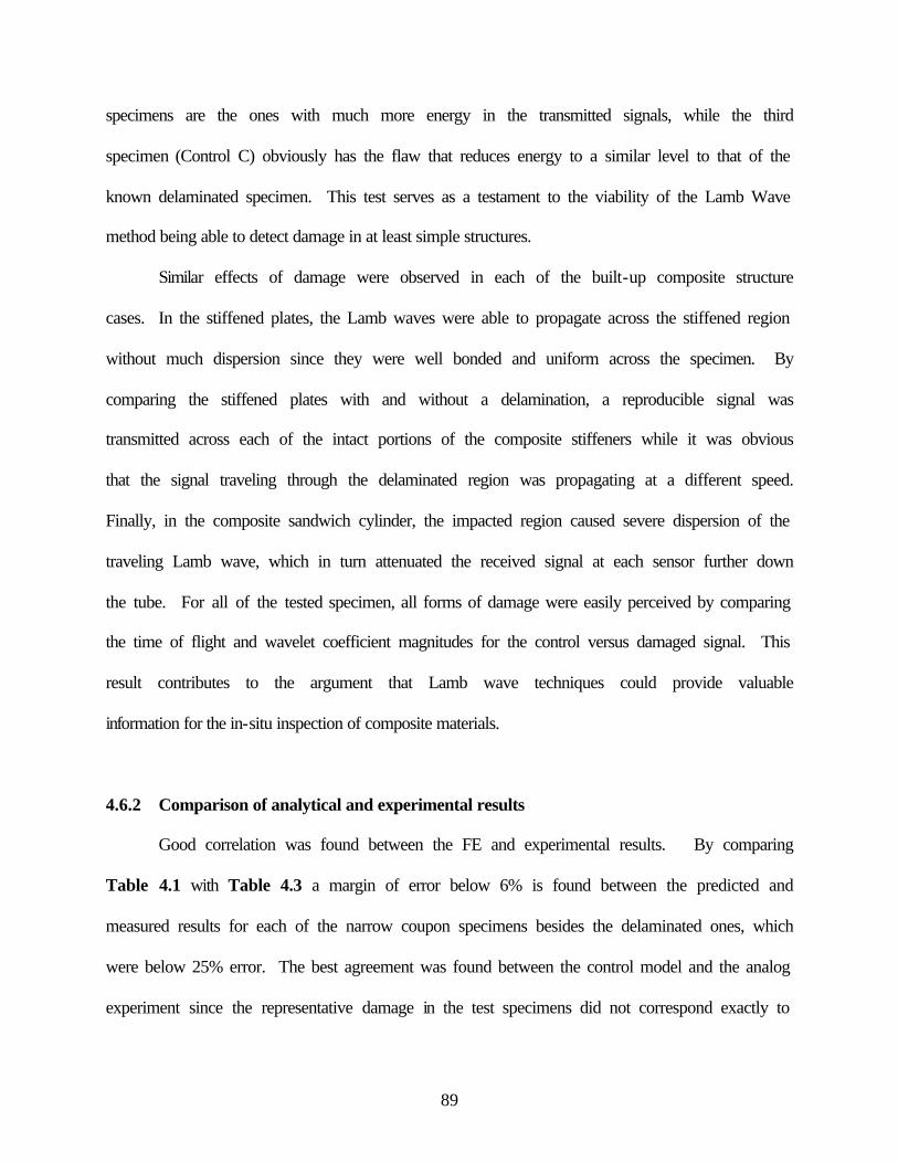
89
specimens are the ones with much more energy in the transmitted signals, while the third
specimen (Control C) obviously has the flaw that reduces energy to a similar level to that of the
known delaminated specimen. This test serves as a testament to the viability of the Lamb Wave
method being able to detect damage in at least simple structures.
Similar effects of damage were observed in each of the built-up composite structure
cases. In the stiffened plates, the Lamb waves were able to propagate across the stiffened region
without much dispersion since they were well bonded and uniform across the specimen. By
comparing the stiffened plates with and without a delamination, a reproducible signal was
transmitted across each of the intact portions of the composite stiffeners while it was obvious
that the signal traveling through the delaminated region was propagating at a different speed.
Finally, in the composite sandwich cylinder, the impacted region caused severe dispersion of the
traveling Lamb wave, which in turn attenuated the received signal at each sensor further down
the tube. For all of the tested specimen, all forms of damage were easily perceived by comparing
the time of flight and wavelet coefficient magnitudes for the control versus damaged signal. This
result contributes to the argument that Lamb wave techniques could provide valuable
information for the in-situ inspection of composite materials.
4.6.2 Comparison of analytical and experimental results
Good correlation was found between the FE and experimental results. By comparing
Table 4.1 with Table 4.3 a margin of error below 6% is found between the predicted and
measured results for each of the narrow coupon specimens besides the delaminated ones, which
were below 25% error. The best agreement was found between the control model and the analog
experiment since the representative damage in the test specimens did not correspond exactly to
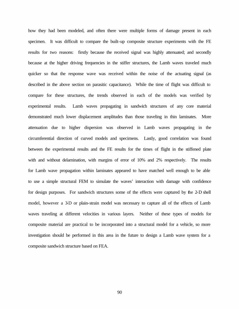
90
how they had been modeled, and often there were multiple forms of damage present in each
specimen. It was difficult to compare the built-up composite structure experiments with the FE
results for two reasons: firstly because the received signal was highly attenuated; and secondly
because at the higher driving frequencies in the stiffer structures, the Lamb waves traveled much
quicker so that the response wave was received within the noise of the actuating signal (as
described in the above section on parasitic capacitance). While the time of flight was difficult to
compare for these structures, the trends observed in each of the models was verified by
experimental results. Lamb waves propagating in sandwich structures of any core material
demonstrated much lower displacement amplitudes than those traveling in thin laminates. More
attenuation due to higher dispersion was observed in Lamb waves propagating in the
circumferential direction of curved models and specimens. Lastly, good correlation was found
between the experimental results and the FE results for the times of flight in the stiffened plate
with and without delamination, with margins of error of 10% and 2% respectively. The results
for Lamb wave propagation within laminates appeared to have matched well enough to be able
to use a simple structural FEM to simulate the waves’ interaction with damage with confidence
for design purposes. For sandwich structures some of the effects were captured by the 2-D shell
model, however a 3-D or plain-strain model was necessary to capture all of the effects of Lamb
waves traveling at different velocities in various layers. Neither of these types of models for
composite material are practical to be incorporated into a structural model for a vehicle, so more
investigation should be performed in this area in the future to design a Lamb wave system for a
composite sandwich structure based on FEA.

91
4.6.3 Role of Lamb wave methods in SHM
Lamb wave techniques have good potential for implementation in a SHM system. These
methods provide useful information about the presence and extent of damage in composite
materials, hold the potential of determining location and type of damage, and can be applied to a
structure with conformable piezoelectric devices. The major disadvantage of this method is that
it is active; it requires a voltage supply and function generating signal to be supplied. This can
be complicated in a large structure, especially if the SHM system is to be implemented
wirelessly; it has been suggested in the literature however that PZT can be actuated remotely
using radio frequency waves [96]. Another difficult requirement is the high data acquisition rate
needed to gain useful signal resolution. If a system is sampling at 0.5 MHz from several sensors,
a large volume of data will accumulate quickly; this implies the need for local processing. The
data acquisition capabilities dictate the limitations of flaw size able to be resolved by a system
using this method. In order to conserve power and data storage space, the Lamb wave method
should most likely be placed into a SHM system in conjunction with another passive detection
method, such as a frequency response method. The piezoelectric patches used to actuate the
Lamb waves could passively record frequency response data until a certain threshold of change
is surpassed, and then trigger the generation of Lamb waves to gain more specific data about the
damaged region. Three to four piezoelectric multi-functioning actuator/sensor patches would be
placed in the same vicinity in order to be able to triangulate damage location based upon
reciprocal times of flight and reflected waves. Another possible scheme could rely on long strips
of piezoelectric material, which would be able to send and receive wide uniform Lamb waves,
and integrate the received and reflected energy in order to determine the state of the material
between them. The separation between sensing patches in either of these configurations would

92
depend on several parameters such as the material properties, damping characteristics and
curvature of the structure, which for flat areas could be as large as 2 meters apart [96]. The
detailed specifications of the Lamb wave driving parameters to be used for a particular
application would be designed by the procedure described in the optimization section.
In the previous discussion sections, it has been shown that there is a good correlation
between FE models and experimental results for Lamb wave propagation, so the effectiveness of
this method in a particular application can be simulated using existing structural models with
slight modifications. Lamb wave methods have demonstrated their effectiveness in detecting the
presence of several forms of damage in a variety of shapes and constructions of composite
components. From these experiments there are indications that these methods should be capable
of measuring the severity, size and location of damage as well. For the delaminated stiffener for
example, by integrating the energy present in a series of time steps the presence of delamination
should be obvious due to the non-uniform wave front, while the fringe pattern in the transmitted
and reflected wave should contain enough information to determine the width of the
delamination. Similarly, for the impacted cylinder case, a time integration of the energy
transmitted would clearly reveal the damage presence. The application of Lamb wave
techniques to a SHM architecture will be discussed further in Chapter 6.
4.7 Conclusions
This chapter has explored the optimization and application of Lamb wave methods to
damage detection in composite materials. A collection of equations is offered in order to
optimize the driving parameters and actuator dimensions for testing. With these tools, an
optimal configuration was selected for the experimental section of this research. Using this

93
procedure, several narrow graphite/epoxy specimens were tested with various forms of pre-
existing damage, such as delamination, matrix-cracks and through–thickness holes. Similar tests
were also performed on narrow sandwich beams using cores of various densities and stiffness.
These tests demonstrated the feasibility of detecting several types of flaws in representative
composite structures, and this method was validated successfully by a “blind test” of several
beam specimens. Tests were also performed on built-up composite structures such as stiffened
plates and curved sandwich structures. Analytical modeling of these specimens yielded similar
results. Lamb wave techniques have the potential to provide more information than previously
tested methods, such as frequency response methods, since they are more sensitive to the local
effects of damage to a material than the global response of a structure. Similar to frequency
response methods, their results are limited at higher frequencies, however their low frequency
results should provide sufficient data to predict damage. The disadvantage of Lamb wave
methods is that they require an active driving mechanism to propagate the waves, and the
resulting data can be more complicated to interpret than for many other techniques. Overall
however, Lamb wave methods have been found to be the most effective for the in-situ
determination of the presence and severity of damage in composite materials of the methods
examined in this thesis.

94
Figure 4.1: Graphical representation of A and S Lamb wave shapes
Figure 4.2: Phase velocity dispersion curve for the Ao mode of an 8-ply composite laminate

95
Determine Material Properties E, ν , ρ , t
Plot phase and group velocity dispersion curves
Choose ω so dcg/dω=0 Or choose ω 10% below A1
Factor in FEA, actuator and data acquisition ω capabilities
Choose actuator dimensions 2a=λ(n+1/2), n=0,1,2…
Experimentally tune optimal ω with driver and oscilloscope
Figure 4.4: Lamb wave actuation frequency selection flow chart
Figure 4.3: Group velocity dispersion curve for the Ao mode of an 8-ply composite laminate
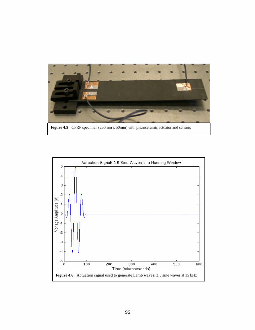
96
Figure 4.5: CFRP specimen (250mm x 50mm) with piezoceramic actuator and sensors
Figure 4.6: Actuation signal used to generate Lamb waves, 3.5 sine waves at 15 kHz

97
Figure 4.7: Sandwich beam specimens (250mm x 50mm) with various cores Listed from top to bottom: high-density aluminum honeycomb, low-density aluminum honeycomb, Nomex and Rohacell
Figure 4.8: Composite plates (250mm x 250mm) with bonded stiffeners. On left, steel C-channel measuring 40mm x 250mm x 20mm. On right, CFRP doublers, 40mm x 250mm x 2mm (16 plies).
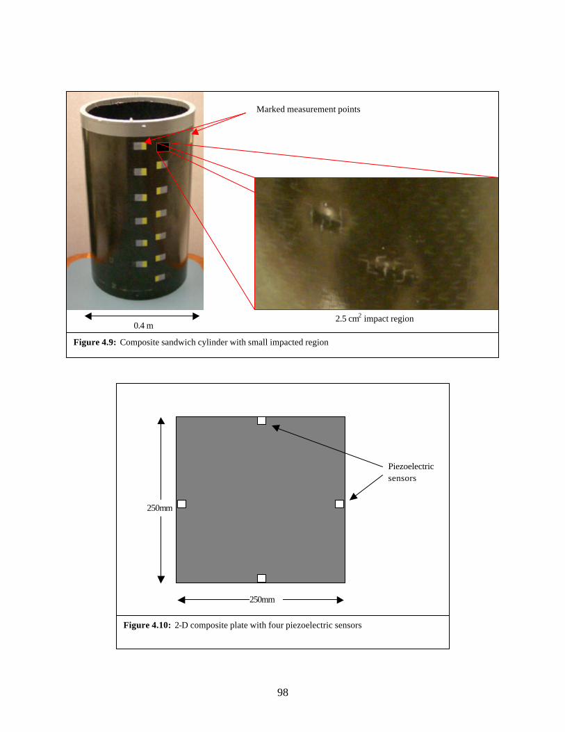
98
0.4 m 2.5 cm2 impact region
Marked measurement points
Figure 4.9: Composite sandwich cylinder with small impacted region
250mm
250mm
Piezoelectric sensors
Figure 4.10: 2-D composite plate with four piezoelectric sensors
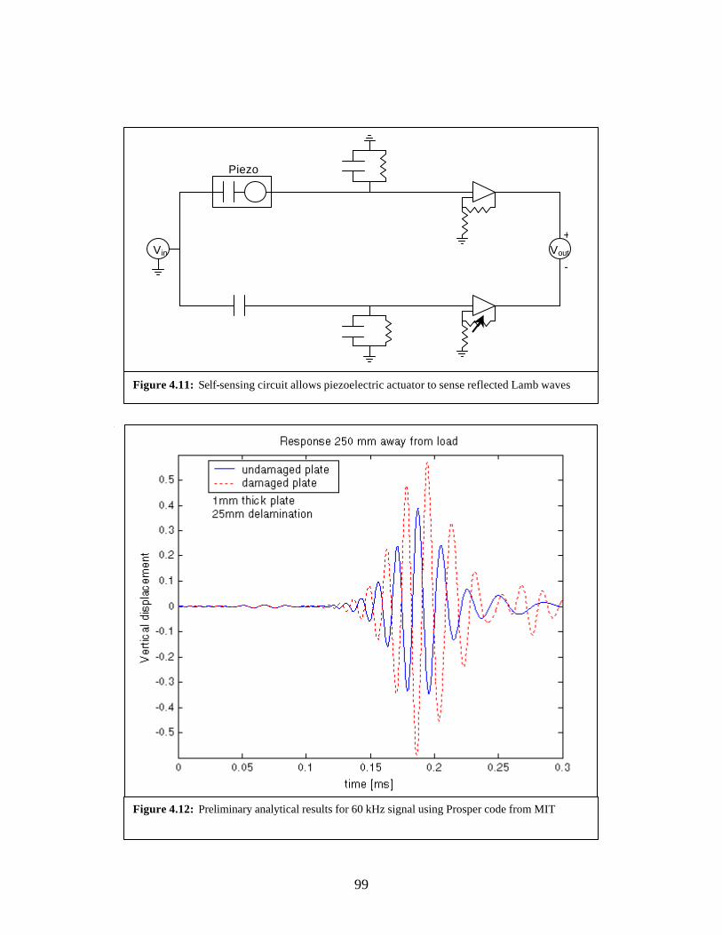
99
+
- Vout
Piezo
Vin
Figure 4.11: Self-sensing circuit allows piezoelectric actuator to sense reflected Lamb waves
Figure 4.12: Preliminary analytical results for 60 kHz signal using Prosper code from MIT

100
Figure 4.13: FEA results for narrow coupon with no damage at 100 microsecond intervals
0 µs
100 µs
200 µs
300 µs
400 µs
500 µs
25 mm
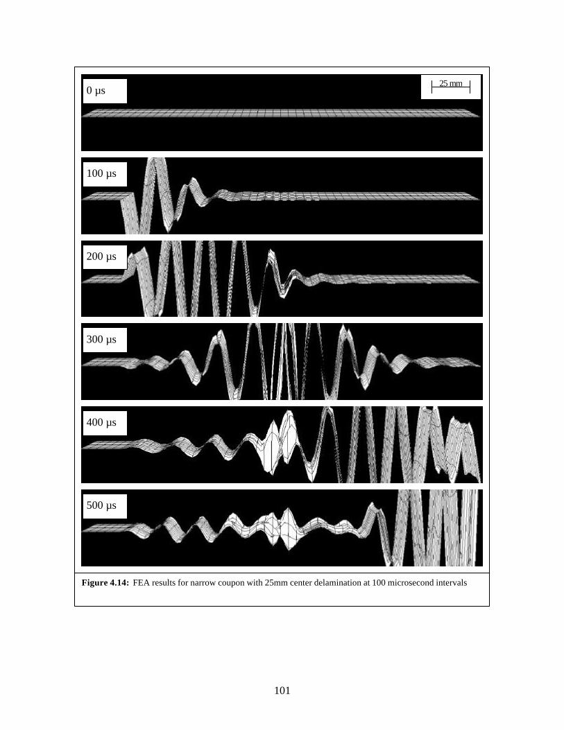
101
Figure 4.14: FEA results for narrow coupon with 25mm center delamination at 100 microsecond intervals
0 µs
100 µs
200 µs
300 µs
400 µs
500 µs
25 mm
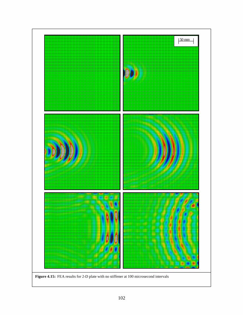
102
Figure 4.15: FEA results for 2-D plate with no stiffener at 100 microsecond intervals
50 mm
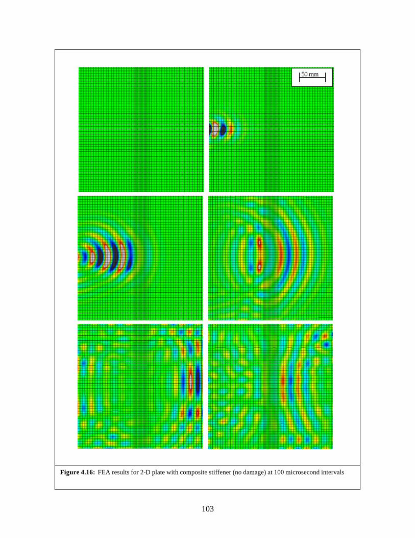
103
Figure 4.16: FEA results for 2-D plate with composite stiffener (no damage) at 100 microsecond intervals
50 mm

104
Figure 4.17: FEA results for 2-D plate with delaminated composite stiffener at 100 microsecond intervals
50 mm

105
Figure 4.18: FEA results for curved sandwich panel with no damage at 10 microsecond intervals
50 mm

106
Figure 4.19: FEA results for curved sandwich panel with impact damage at 10 microsecond intervals
50 mm
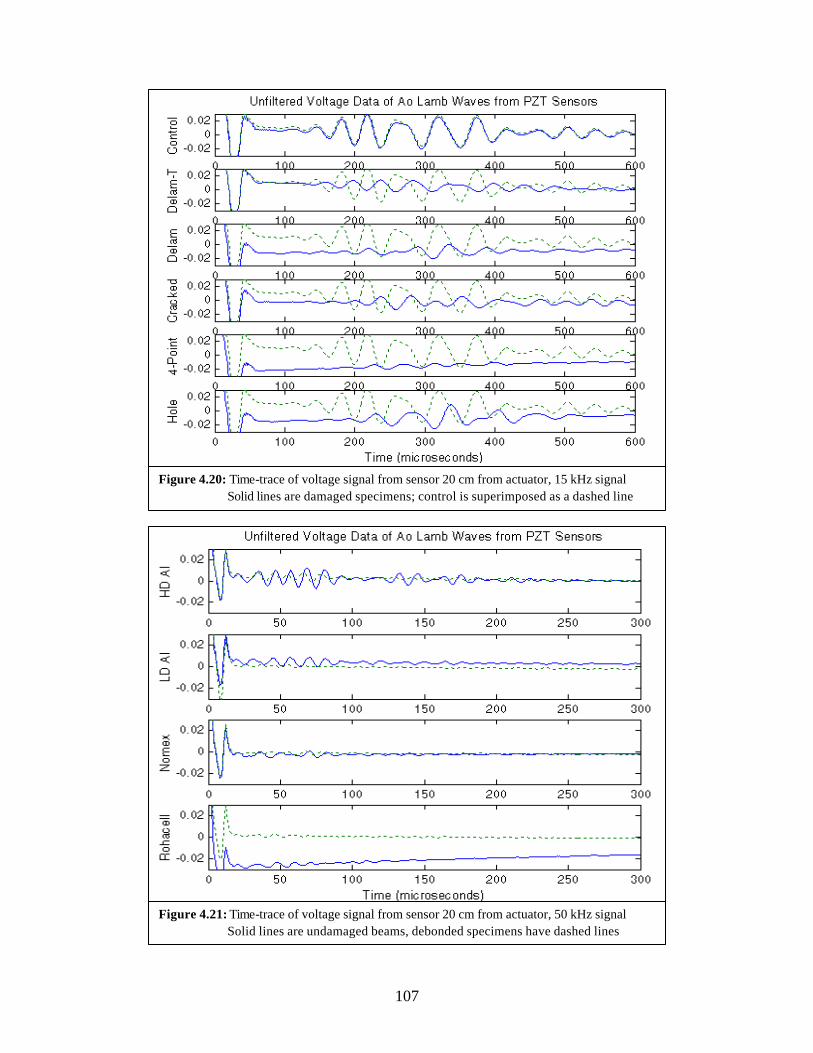
107
Figure 4.20: Time-trace of voltage signal from sensor 20 cm from actuator, 15 kHz signal Solid lines are damaged specimens; control is superimposed as a dashed line
Figure 4.21: Time-trace of voltage signal from sensor 20 cm from actuator, 50 kHz signal Solid lines are undamaged beams, debonded specimens have dashed lines

108
Figure 4.22: Wavelet coefficients for thin coupons; compares 15 kHz energy content
Figure 4.23: Wavelet coefficients for beam “blind test”; compares 50 kHz energy content

109
Figure 4.24: Time-trace of voltage signal for stiffened plates, 15 kHz signal
Figure 4.25: Wavelet coefficients for stiffened plates; compares 15 kHz energy content

110
Figure 4.26: Time-trace of voltage signal for composite sandwich cylinder, 40 kHz signal
Figure 4.27: Wavelet coefficients for composite cylinder; compares 40 kHz energy content

111
Figure 4.28: Time-trace and wavelet coefficients for circumferential scan, 40 kHz signal
Figure 4.29: Time-trace of voltage signal for impacted cylinder, 40 kHz signal

112
Figure 4.30: Wavelet coefficients for impacted cylinder; compares 40 kHz energy content
Figure 4.31: Time-trace of voltage signal for 2-D plate, 15 kHz signal. Each plot represents actuation from a different side. Blue curve is sensed wave directly across from actuator. Red and green curves are sensed waves on sides adjacent to actuator.
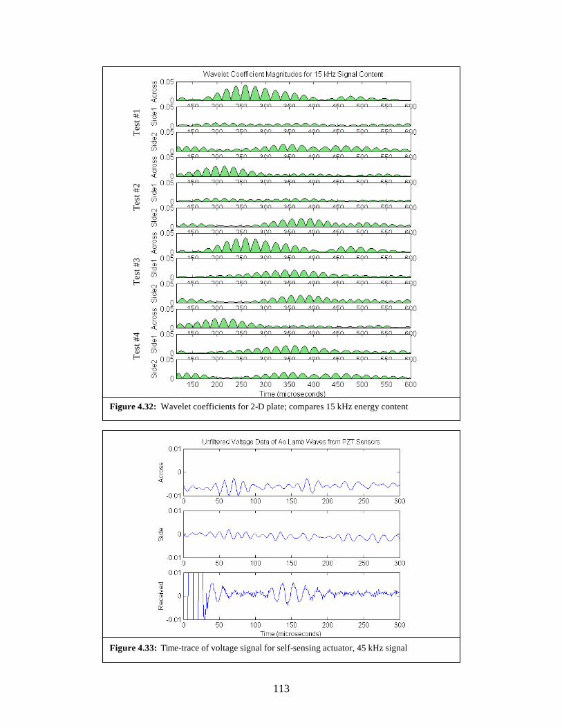
113
Figure 4.33: Time-trace of voltage signal for self-sensing actuator, 45 kHz signal
Figure 4.32: Wavelet coefficients for 2-D plate; compares 15 kHz energy content
Tes
t #1
Tes
t #2
Tes
t #3
Tes
t #4

114
(times in microseconds, velocities in m/s)
TOF based on initial arrival
TOF based on peak arrival
Cg based on initial arrival
Cg based on peak arrival
∆t from undamaged
High density Al 26 26 7910 7910 - High density Al w/delam 32 36 6430 5720 6 Low density Al 45 43 4572 4780 - 2-D plate 318 290 647 709 - 2-D plate w/CFRP rib 308 310 668 664 -10 2-D plate w/CFRP rib delam 314 300 655 686 -4 2-D plate w/steel c-channel 308 290 668 709 -10 (times in microseconds, velocities in m/s)
TOF based on initial arrival
TOF based on peak arrival
Cg based on initial arrival
Cg based on peak arrival
∆t from undamaged
Undamaged 216 218 952 944 - Center cracked region 238 233 864 883 22 Center 5mm hole 226 230 910 894 10 Center 50x50mm delam 261 258 788 797 45 Side 50x25mm delam 231 220 890 935 15
(times in microseconds, velocities in m/s)
TOF based on initial arrival
TOF based on peak arrival
Cg based on initial arrival
Cg based on peak arrival
∆t from undamaged
Undamaged 230 230 894 894 - Center cracked region 231 231 891 891 1 Center 5mm hole 237 231 868 891 7 Center 50x50mm delam 306 280 672 735 76 Side 50x25mm delam 292 354 704 581 62
(times in microseconds, velocities in m/s)
TOF based on initial arrival
TOF based on peak arrival
Cg based on initial arrival
Cg based on peak arrival
∆t from undamaged
High density Al 24 27 8570 7620 - High density Al w/delam 30 31 6860 6640 6 Low density Al 30 37 6860 5560 - Low density Al w/delam 37 41 5560 5020 7 Nomex 36 35 5720 5880 - Rohacell 27 28 7620 7350 -
Table 4.2: Lamb wave times of flight and group velocities for all geometries as observed from FEM solutions
Table 4.1: Lamb wave times of flight and group velocities for narrow coupons as observed from FEM solutions
Table 4.3: Lamb wave times of flight and group velocities for narrow coupons as observed experimentally
Table 4.4: Lamb wave times of flight and group velocities for sandwich beams as observed experimentally

115
Chapter 5
OTHER PIEZOELECTRIC-BASED SENSING METHODS
There are many advantages to using piezoelectric sensors in SHM applications; they are
light, can be conformable, use little power and are sensitive to small strains and accelerations.
The two previous chapters of this thesis have given a detailed account of the frequency response
and Lamb wave methods using piezoelectric sensors and actuators. Both of these methods have
demonstrated useful sensitivity to damage, however they are most effectively implemented
actively by using powered actuators in a pulse-transmission or pulse-echo mode. Perhaps the
greatest advantage of using piezoelectric material for sensors, is that they can be used for a wide
variety of detection techniques by simply altering the time scale of analysis or actuating signal.
This chapter gives an overview of two further techniques, acoustic emission and strain
monitoring, which could be implemented via the piezoelectric sensors and system infrastructure
used for the previous two methods presented, to detect damage passively without the use of
actuators. These methods can offer supplemental information about the state of the structure,
while only requiring some additional software. Background for these methods are presented
from the literature, as well as results from simple proof of concept experiments that were
performed.

116
5.1 Background
As mentioned previously in Chapter 2, one of the earliest forms of damage monitoring in
vehicles involved observing strains using resistive foil gauges. These sensors are applied easily
to the surface of a structure, and output data that is simple to analyze with little processing.
Operators have used records from strain gauges to check for over-strains in components, as well
as to calculate stresses based on stiffness estimations [7]. Optical fibers have been embedded in
composite structures to serve the same purposes over a distributed area with slightly more
complexity [154]. More recently, piezoelectric sensors have been considered for the in-situ
monitoring of operational strains. There have been a few articles in the literature that have
suggested piezoelectric sensors for this role. Rees et al suggested the use of piezoelectric patch
sensors placed around a boron/epoxy repair site to monitor cracks growing in the epoxy [155]. A
finite element approach was used to show the strain increase from the stress concentration
developing under the sensor as the crack grew. A sensitivity study showed that cracks larger
than 11 mm would be able to be detected by this scheme. The majority of this work was
analytical, however experimental validation was provided in a second paper that showed the
detection of a 10x10 mm disbond in a boron/epoxy repair patch adhered to an aluminum
structure [156]. This study also concluded that the impedance properties of the piezoelectric
sensor would start to degrade above 2000 microstrain. Moreover, in another experimental paper,
Hautamaki et al have fabricated and demonstrated a series of MEMS piezoelectric sensors,
which exhibited linear results through 1000 microstrain [157]. Strain based damage monitoring
methods have shown potential to detect cracks on the order of a centimeter in length, however
their results are localized to the area beneath the sensors which would require many more sensors
for vehicle coverage as compared to frequency response or Lamb wave methods.

117
Another commonly implemented use of piezoelectric sensors for damage detection in
composite structures has been acoustic emission. This method has become well accepted since it
does not require actuation, and its results can provide better information regarding damage
location than most other techniques. In its simplest form, this method involves measuring the
time of flight of a circular pattern of stress waves emanating from a point source; depending on
the sensitivity of the system, this point source could be an impact event or a fiber breaking.
Often resonant sensors are designed so that they are tuned to the expected frequency of particular
forms of damage to amplify their presence while other ambient vibrations are damped out [32].
Several researchers have investigated this and other techniques in the literature [29, 158-160].
The reason why acoustic emission has not become standard practice is because of the
complexities that arise from wave propagation in composite materials. Analytically the
triangulation of a damage detection site can be easily calculated in an elastic isotropic material
based on time of flight measurements, however in anisotropic and inhomogeneous composite
materials these waves do not behave perfectly, and there can be much dispersion and attenuation
due to the fiber structure that distorts the signals and makes a damage location prediction
difficult. Chang’s group at Stanford has had the most success in this field [161]. In their smart-
structures program, they have successfully been able to determine the location of an impact even
in stiffened composite panels to within 10% accuracy with sensors spaced about 25 cm apart, by
using a model-based approach. The metric for the type and size of damage detectable by
acoustic emission differs significantly from most techniques however, since this method is based
on the amount of energy being released by an impact event or crack propagation, and it can only
be detected while that energy is being released. This is compared to the three previous methods
described in this thesis, which can be queried to search for the presence of damage at any instant
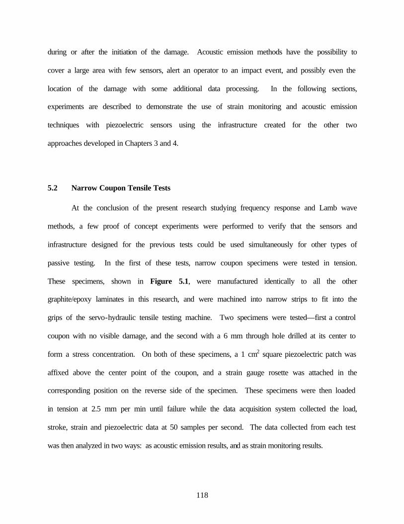
118
during or after the initiation of the damage. Acoustic emission methods have the possibility to
cover a large area with few sensors, alert an operator to an impact event, and possibly even the
location of the damage with some additional data processing. In the following sections,
experiments are described to demonstrate the use of strain monitoring and acoustic emission
techniques with piezoelectric sensors using the infrastructure created for the other two
approaches developed in Chapters 3 and 4.
5.2 Narrow Coupon Tensile Tests
At the conclusion of the present research studying frequency response and Lamb wave
methods, a few proof of concept experiments were performed to verify that the sensors and
infrastructure designed for the previous tests could be used simultaneously for other types of
passive testing. In the first of these tests, narrow coupon specimens were tested in tension.
These specimens, shown in Figure 5.1, were manufactured identically to all the other
graphite/epoxy laminates in this research, and were machined into narrow strips to fit into the
grips of the servo-hydraulic tensile testing machine. Two specimens were tested—first a control
coupon with no visible damage, and the second with a 6 mm through hole drilled at its center to
form a stress concentration. On both of these specimens, a 1 cm2 square piezoelectric patch was
affixed above the center point of the coupon, and a strain gauge rosette was attached in the
corresponding position on the reverse side of the specimen. These specimens were then loaded
in tension at 2.5 mm per min until failure while the data acquisition system collected the load,
stroke, strain and piezoelectric data at 50 samples per second. The data collected from each test
was then analyzed in two ways: as acoustic emission results, and as strain monitoring results.
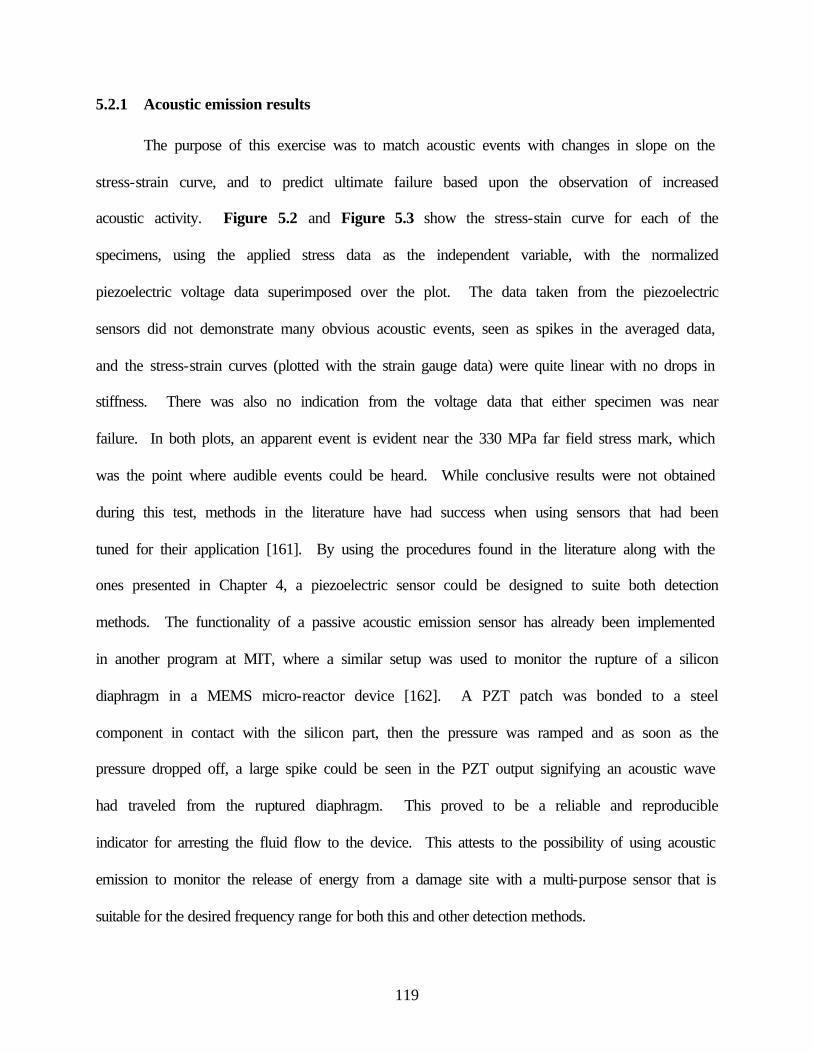
119
5.2.1 Acoustic emission results
The purpose of this exercise was to match acoustic events with changes in slope on the
stress-strain curve, and to predict ultimate failure based upon the observation of increased
acoustic activity. Figure 5.2 and Figure 5.3 show the stress-stain curve for each of the
specimens, using the applied stress data as the independent variable, with the normalized
piezoelectric voltage data superimposed over the plot. The data taken from the piezoelectric
sensors did not demonstrate many obvious acoustic events, seen as spikes in the averaged data,
and the stress-strain curves (plotted with the strain gauge data) were quite linear with no drops in
stiffness. There was also no indication from the voltage data that either specimen was near
failure. In both plots, an apparent event is evident near the 330 MPa far field stress mark, which
was the point where audible events could be heard. While conclusive results were not obtained
during this test, methods in the literature have had success when using sensors that had been
tuned for their application [161]. By using the procedures found in the literature along with the
ones presented in Chapter 4, a piezoelectric sensor could be designed to suite both detection
methods. The functionality of a passive acoustic emission sensor has already been implemented
in another program at MIT, where a similar setup was used to monitor the rupture of a silicon
diaphragm in a MEMS micro-reactor device [162]. A PZT patch was bonded to a steel
component in contact with the silicon part, then the pressure was ramped and as soon as the
pressure dropped off, a large spike could be seen in the PZT output signifying an acoustic wave
had traveled from the ruptured diaphragm. This proved to be a reliable and reproducible
indicator for arresting the fluid flow to the device. This attests to the possibility of using acoustic
emission to monitor the release of energy from a damage site with a multi-purpose sensor that is
suitable for the desired frequency range for both this and other detection methods.

120
5.2.2 Strain monitoring results
The second way the data was analyzed was to assess the accuracy of the piezoelectric
sensors for the measurement of strain by contrasting them to the foil-gauge results, again as
shown in Figure 5.2 and Figure 5.3. The stress-strain curves using the strain gauge data were
very linear, however the curves using the PZT data was significantly nonlinear. These curves
could be divided into three regions which are roughly linear in themselves, however the
significance of these regions in not readily obvious. As described in the previous background
section, many piezoelectric materials only respond linearly to strain below certain limits, such as
1000 microstrain, and while the test presented in this section was preformed at a much lower
strain level, the PZT used as the sensor in the test had not been previously characterized for its
linear strain limit since the strains due to Lamb waves were extremely low. A more reasonable
explanation attributes this non-linearity to the thermoplastic tape that attached the sensor to the
specimens. The first linear region most likely corresponded to the data up until the linear-elastic
limit of the thermoplastic, followed by the second in its plastic region and then the final region
where the tape was beginning to detach from the specimen. Upon failure of the specimen, the
sensor completely detached itself from the composite leaving all of the thermoplastic attached to
the copper on the back of the sensor, indicating that at the time of failure there was not a good
bond between the sensor and the specimen. Again, this test did not provide conclusive results,
however as demonstrated in the literature, piezoelectric materials have been used to monitor
strain, and with some more experimentation with attachment method to be employed and the
determination of the proper linear region for the sensor selected, it should be possible to use
piezoelectric sensors for direct strain measurement within the infrastructure of other testing
methods that have been presented in this thesis.

121
5.3 2-D Plate Tests
A second set of tests was performed on a laminated plate in order to further explore the
feasibility of using the PZT sensors from the present research to monitor damage events
passively, and attempt to perform a triangulation to locate the damaged area. The graphite/epoxy
laminate used for the 2-D plate Lamb wave tests in Chapter 4 was re-used for these tests, with
the four sensors patches affixed in the same locations in the center of each of the sides along the
perimeter. Data was collected at 50 Hz (so as not to generate a large volume of data points) as a
graphite pencil tip was broken in several locations on the laminate in a clockwise fashion, shown
in Figure 5.4, as is common practice for acoustic emission verifications tests. The data was
sampled simultaneously from each of the 4 sensors in order to attempt to triangulate the location
of the pencil break using the previously calculated characteristic speed in this laminate from
Chapter 4. The voltage results from these tests are plotted in Figure 5.5, and Figure 5.6 shows
the wavelet decomposition of these signals. From the voltage plots, one can see the acoustic
event within the signal by the voltage spike present following each pencil break. At this data
sampling rate however, it was not possible to resolve the arrival times of the voltage spikes
accurately enough to perform a triangulation calculation. A reasonable prediction of the pencil
break site could be made from wavelet plots though, by comparing the magnitude of the energy
present for each sensor at the time of the breakage. In Figure 5.5 for example, it can be seen that
for the first test where the pencil was broken once near each sensor, that event excited the largest
response from the adjacent sensor since the traveling acoustic wave would have attenuated
before reaching the other sensors. The same can be seen for the second test shown in Figure 5.6
where the pencil was broken between a pair of sensors, and these pairs consistently exhibited the
largest response. From these comparisons, an estimate could be made as to the proximity of the

122
damage to each sensor. Using the present infrastructure and sensors suggested in Chapters 3 and
4 for the frequency response and Lamb wave methods, once a threshold value is surmounted to
trigger the system, a comparison could be made between the magnitude of received energy at
each sensor to predict the location of an impact event. If a higher data acquisition rate was
available to the system, much more information regarding the damage location would be evident
using the time of arrival data.
5.4 Discussion
The purpose of this chapter was to introduce other damage detection methods that could
be performed within the infrastructure of piezoelectric sensors and the data acquisition system
used for the frequency response and Lamb wave methods presented in Chapters 3 and 4 of this
thesis. The first method considered in this chapter was the strain monitoring of specimens. By
measuring the peak strain witnessed at the surface of a laminate, a prediction of failure can be
made based upon the strain limitations of the material. The specific results in the current
experiments did not provide sufficiently consistent information to make these predictions,
however several researchers in the literature have successfully fabricated piezoelectric based
strain gauges that are valid for certain strain rates and ranges. Additional research would have to
be performed to find a more appropriate attachment mechanism for this method to be successful.
Similarly, the second method, which focused on acoustic emission, did not provide as much
information as previous researchers have reported with similar techniques, which is due to the
slow data acquisition rate and non-optimal sensor configuration. As presented in the background
section, prior successful acoustic emission work has been performed using sampling rates
between 300 kHz and 3 MHz, however for the current setup these sampling rates were not

123
practical for continuous monitoring because of the amount of data that would have been
produced. Previous researchers have bypassed this problem by using an instrumented striking
device to trigger the system to capture a small buffer worth of data points at very short time
steps. To monitor continuously without a trigger, custom software would have to be used along
with complex hardware, in order to collect small buffered series of data at high acquisition rates,
and then scan that data for voltage spikes while collecting the next buffer full of data. This
process would have to take place very quickly and efficiently so that the non-essential buffered
data could be purged from the system before a large volume of useless data began to fill the
storage device. Regardless, acoustic emission methods have shown the potential to provide
valuable information concerning the occurrence of an impact event and proximity to the sensor.
Although the experimental results presented in this chapter were not conclusive, coupled
with the results presented in the literature this preliminary data demonstrated the possibility that
the piezoelectric sensors could passively collect useful data with some additional software and
data processing capabilities. The most encouraging result came from the wavelet decomposition
of the pencil break test, which clearly indicated the occurrence of each breakage event, and by
comparing the wavelet energy magnitudes provided information to help deduce the impact
location. One proposed system architecture could perform these methods passively, by using
sensors that are present for other detection methods, to obtain early warning signs of damage
such as an impact event or a higher than ordinary strain level. Subsequently, the system could
then respond by using more robust methods, such as transfer-function frequency response or
Lamb waves, to more aggressively pinpoint the type and location of damage. These ideas will be
further elaborated upon within Chapter 6, which describes the other components of an SHM
system and provides suggestions for a successful system architecture.

124
Figure 5.2: Rotated stress-strain plot for control coupon, piezo voltage data superimposed
Figure 5.1: Narrow coupon tensile specimen with strain gauge rosette and piezo sensor attached
Front side Back side
Data Acquisition
Strain Gauge Piezoceramic
250 mm
Piezo sensor data
Foil gauge data

125
Figure 5.3: Rotated stress-strain plot for coupon with hole, piezo voltage data superimposed
Figure 5.4: Acoustic emission setup. Pencil break points for tests #1 and #2 are labeled
250mm
250mm
Piezoelectric sensors
Test #1 break point
Test #2 break point
Both tests break point
Piezo sensor data
Foil gauge data

126
Figure 5.5: Time-trace of voltage signal recorded by each piezo for tests #1 and #2
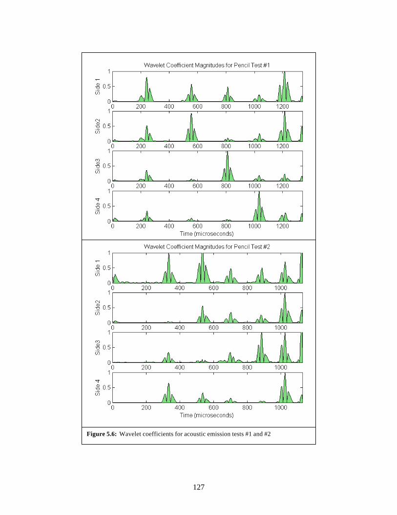
127
Figure 5.6: Wavelet coefficients for acoustic emission tests #1 and #2

128
[This page intentionally left blank]

129
Chapter 6
STRUCTURAL HEALTH MONITORING SYSTEMS
In the previous chapters of this thesis, the concept of a Structural Health Monitoring
system was introduced, and the motivation for implementing one was presented. The focus until
this point has been on sensors and sensing methods, concentrating mostly on piezoelectric based
methods such as frequency response and Lamb waves. This chapter delineates the relevant
considerations and components necessary for a complete SHM system. It continues with
recommendations for implementation of SHM within composite structures based on the present
research, and concludes with a discussion of possible directions for the future of SHM systems.
6.1 Components of SHMS
This section introduces the necessary components of a SHM system. The focus of the
previous chapters of this thesis has been on the sensors used for the actual damage detection in
the structure, however perhaps of equal importance and challenge are the other components used
to convert, process and transmit the data from these sensors. An overall SHM system
architecture is necessary to integrate strategically all of the other components for the most
efficient operation. Characteristic damage signatures must be known for the particular material
and structure to select appropriate sensors and sensing methods. The data from the sensors must
be communicated between the sensors and to a processing unit, and algorithms are needed to
130
interpret this data. Some systems may require an intervention component as well. All of these
components must work together to gather the information about damage in the structure, and
flawlessly relay this information to an operator for the system to work reliably.
6.1.1 Architecture
The architecture of a SHM system is not a particular physical component, nevertheless it
is an important preliminary consideration for the design process. The requirements of the end
users are incorporated into the architecture in order to define the types of damage to be
monitored, the critical flaw size, the weight and power budget for the system, and the level of
importance of the various structural members that need to be monitored. It includes the layout of
where the physical components of the SHM system lie and how they interact. One decision is
the choice between a real-time (continuous) and discontinuous SHM system. A real-time SHM
system is one that continually monitors a structure during operation, and produces data that can
be directly utilized at any point by either an operator or ground control station. A discontinuous
SHM system is one that data can only be accessed post-operation and could contain either a
stored record of operational health data or might involve performing an integral inspection upon
demand. Discontinuous systems are much less complex than real-time ones since much of the
infrastructure needed to power, transfer and analyze the damage detection data can be contained
in an external unit that is used to access key in-situ components. Additionally the level
redundancy for each component needs to be assigned to achieve a desired level of reliability in
catching false-positives as well as true-positives.
There are several other questions a SHM system designer encounters when specifying the
architecture. Is the system to be designed for an aging or new vehicle? What material is being

131
used for the structure? Should the system be embedded or surface mounted? The designer must
also determine the sensor placement density and pattern; the more sensors the better the damage
resolution, with increased power and weight as penalties. One architectural concept introduced
in this chapter is that of the SHM patch. This scheme clusters several sensors and other
components together to be incorporated on the structure to operate independently of other
patches. A few suggested systems architectures can be found in the literature, with one thorough
description given by Ikegami from Boeing [163]. In this paper, he provides flow charts for the
transfer of data between the various components and provides suggestions for implementation.
6.1.2 Damage characterization
Damage characterization might be considered a subsystem of the architecture, however it
is sufficiently important to be discussed in depth. This is probably the most fundamental aspect
of detecting damage; the familiarity of what kinds of damage are common in a type of material,
and the knowledge of what “changes” correspond to these forms of damage. These damage
characteristics are dependent on the type of material the structure is manufactured with, as well
as the structural configuration. With metallic structures, designers are mostly concerned with
fatigue cracks and corrosion, while for composite materials, delamination and impact damage are
more of a concern. Structural configuration includes secondary structures that may introduce
new areas for damage to exist, or influence the effect of damage on the primary structure.
Examples of this include core materials or stiffeners in a composite structure that can delaminate,
and ribs or fasteners in metallic structures that can introduce stress concentrations or crack
initiation sites. Once an understanding of the damage signature in the material of concern is
reached, then the sensing method and sensors can be selected.
132
6.1.3 Sensors
Sensors are used to record variables such as strain, acceleration, sound waves, electrical
or magnetic impedance, pressure or temperature. Previous chapters have gone into depth
describing some of the sensing systems with the most potential for damage detection, including
frequency response, Lamb wave, acoustic emission and strain monitoring methods. In the
literature it has been estimated that a SHM system for an aerospace vehicle would require
between 100 and 1000 sensors, depending on its size and desired coverage area [29]. Sensing
systems can generally be divided into two classes: passive or active sampling. Passive sampling
systems are those that operate by detecting responses due to perturbations of ambient conditions
without any artificially introduced energy. The simplest forms of a passive system are witness
materials, which use sensors that intrinsically record a single value of maximum or threshold
stress, strain or displacement. Examples of this can be phase change alloys that become
magnetized beyond a certain stress level, shape memory alloys, pressure sensitive polymers, or
extensometers. Another type of passive sensing is strain measurement by piezoelectric wafers.
Lastly, several vibrational techniques can be performed passively, such as some accelerometers,
ambient frequency response and acoustic emission with piezoelectric wafers. Active sampling
systems are those that require externally supplied energy in the form of a stress or
electromagnetic wave to properly function. A few strain-based examples of active systems
include electrical and magnetic impedance measurements, eddy currents and optical fibers which
require a laser light source. Active vibrational techniques include the transfer function modal
analysis and Lamb wave propagation. Good references for selection of actuators for various
active systems can be found in a review paper in the literature [164]. Passive techniques tend to
be simpler to implement and operate within a SHM system and provide useful global damage

133
detection capabilities, however generally active methods are more accurate in providing
localized information about a damaged area. A comparison of the sensing methods can be seen
in Table 6.1. Sensor selection charts plotting size of detectable damage against sensor size and
power requirement for various coverage areas, can be found in Figure 6.1 and Figure 6.2. It can
be seen that they are all generally capable of detecting the same size of damage and can be
implemented with similar size and power sensors, however frequency response and Lamb wave
techniques are the only ones that can offer full surface coverage for a 1 x 1 m plate. While some
other methods, such as eddy currents, can offer better damage resolution, they are only capable
of detecting damage directly below the sensor, which would drive the system to use either very
large sensors or a large volume of sensors.
All of the aforementioned sensing systems have some merit for implementation in an
SHM system. Frequency response methods can be used either actively or passively, Lamb wave
methods are purely active and acoustic emission and strain measurements are typically passive
methods. All of the methods presented in the present work utilize piezoelectric sensors since
they are easy to integrate or embed into a structure, they are low power and fairly robust, making
them a good choice for a composite structure. There are other sensors available for these
methods, which could be suitable depending on the application or the material being monitored.
Many of the other systems mentioned in this section however, require specialized sensors
designed solely for their application, most notably eddy currents and optical fibers.
6.1.4 Computation
Several processing units are necessary to operate a SHM system. On the local level, a
processor must interface with the sensors to acquire the data and convert the raw analog signals

134
to digital ones. If it is an active system, such as with Lamb wave methods, the processor must
send instructions or waveforms to the actuator periodically. Data rates between 25 and 50
Megabytes per second would be necessary for each Lamb wave sensor collecting data in the
system, or 0.5 to 1 Megabytes per second for acoustic emission sensors [29]. At these rates, it
can be seen that a large data storage capacity would become necessary for continuous monitoring
if the data is not immediately processed in a buffer and then overwritten, however a single Lamb
wave test would only use 50 kilobytes. Once the information is collected, the useful, or
“changed” data must be separated from the large quantity of collected data to send to the
processing unit. Compression may be utilized at this step to condense the output signal for
transmission. Local processing may also be necessary to compare data between neighboring
sensor patches for damage verification. There are also global computational needs to use
algorithms to assess the severity of damage, triangulate damage locations or make failure
predictions, and to convey this information to the end-user.
6.1.5 Communication
Another important component of a SHM system is a communication system. This
involves the transfer of data in one form or another between various components of the system.
There are essentially four areas where the transfer of data is necessary: intra-patch, inter-patch,
patch-processor and processor-operator. Intra-patch communications refers to the transfer of
data, either analog or digital form, between various components within a local sensor patch. This
might include the passing of data from the sensor to data acquisition board, an analog-to-digital
converter, or possibly a local processor chip for preliminary data analysis. These transfers would
most likely be across metallic wires or optical fibers since they would only be traveling a short

135
distance, on the order of a few centimeters to a meter at most, and there could be many sensors
involved. The next category is inter-patch communications, which refers to the transfer of
information between various patches in different regions. In some SHM schemes, it would be
beneficial for local sensor sites to be able to communicate in order to compare or verify data and
increase reliability. Inter-patch communication could also be a means to pass data down the line
along a large structure, sacrificing speed for lower power requirements. Most of this category
would be performed with low power wireless transfers over a few meters, so that the various
patches could be installed and operate independently. Next, patch-processor communication is
necessary to transfer the collected sensor data to a central processing unit. To maintain
efficiency, only important data would be transferred to the central computer, which could be
located with the vehicle avionics. Most likely a high-powered wireless method would be
necessary to transfer the data to the computer which could be tens of meters away, unless the
patches were to pass the information along in a data-bus fashion. Lastly, data must be passed
between the processor and the end user to convey information about the state of the structure.
6.1.6 Power
Most of the components mentioned in the previous sections require power to function.
Lamb wave actuators, for example, operating actuating at 15 kHz with 5 V peak-to-peak would
draw 24 mW (using P=2πfCV2). A low power micro-computer to process the data would likely
draw about 10 mW, and a short range wireless device would require about 5 mW to function.
This becomes difficult when there are many components distributed throughout the surface of
the structure, some of which can even be embedded within the skin. Power could be supplied
locally by batteries, or provided from within the vehicle via an electrical bus. Some researchers

136
have proposed systems where energy is transmitted by radio frequencies to inductive loops, or
collected passively with energy harvesting devices to the local sensor and processing patches.
Power systems for SHM systems are probably the least developed area currently.
6.1.7 Algorithms
Algorithms are probably the most essential component to a SHM system. They are
necessary to decipher and interpret the collected data, and require an understanding of the
operational environments and material thresholds. Examples of algorithms that have been
mentioned in this thesis include codes that perform modal analysis and wavelet decomposition.
Other algorithms that could be embedded into a SHM system include codes that interpret the
sensor data to specify the damage size and location, codes that calculate the residual strength or
stiffness of the structure, or codes that predict failure based upon the measured damage. The
accuracy and robustness of the system is dependent on how well these codes are written.
6.1.8 Intervention
The last potential component of a SHM system is some form of intervention mechanism.
Current intervention usually involves a mechanic performing a prescribed repair. Future
advanced intervention systems mechanisms may use the collected damage detection data to
mitigate further damage actively, or possibly even temporarily or permanently repair the damage
site. Some proposed ways of achieving this intervention include the use of shape memory alloys
to stiffen particular areas in the wake of a crack, or inserting epoxy reservoirs or duel phase

137
matrices into a composite to close punctures in the structure. These types of mechanisms are
ideal for future SHM systems, but are not required for useful preliminary ones in the near future.
6.2 Recommendations of Implementation of SHMS in Composite Structures
The main focus of this thesis is to provide design recommendations and guidelines for the
implementation of a structural health monitoring system in a composite structure. The previous
sections of this chapter have explained the required components of SHM systems, and this
section will propose an architecture to connect these components. In order for the system to be
viable, the design must be based on the optimization of a cost function. Sensors and actuators
would be chosen based upon the material to be monitored and the structural configuration,
similar to the description in Chapter 4 for the optimization of Lamb wave sensors. A smart
design will use several different sensing methods, taking advantage of both the strengths and
weaknesses of each; for example certain methods work only in conducting materials and other in
insulating ones, so potentially, damage to fibers could be differentiated from damaged matrix in
a composite by using both concurrently. The trade between redundancy and reliability is
essential since missed damage or false-positives could prove financially fatal to SHM systems.
By using event-driven processing, such as a passive system triggering a dormant active one, a
low duty cycle would save power and complexity. Further gains could be made by taking
advantage of ambient conditions to provide power or actuation. As previously mentioned, good
algorithms designed for the particular material being monitored is key. Lastly, it would be
advantageous to design a system that was flexible enough that it could be retrofitted to existing
aging systems as well as work on new structures.
A design proposed by the author would use relatively small (0.25 - 1.0 m2) autonomous
sensor patches as its key elements. These patches would include multiple piezoelectric sensors

138
around their perimeter, local wiring between the sensors (longest length of 0.5 m), a data
acquisition/processing device (capable of sampling around 1 MHz), a rechargeable polymer
battery with an inductive coil for power reception (50 mW required to power all components),
and a short range wireless device (10 m transmission range). All of these components would be
embedded deposited onto a conformable insulating polymer sheet with a thermoplastic adhesive
backing so that it could easily be applied over any surface of a vehicle. Thermoplastic would be
used to avoid the complexity of an autoclave cure, and so the patch could be removed if it were
damaged or if the surface it was mounted over required repair. Other sensor types could possibly
be deposited onto the polymer as well in certain regions, such as meandering wires for eddy
current tests or differential parallel metal tracks for thermocouple readings. These patches would
be generic so that they could be placed in any region of concern on a vehicle, and could even be
placed on a dispenser like roll to be torn off and applied. Since thermoplastics are removable,
patches could even be replaced if a section becomes damaged or is malfunctioning. Once
attached to the structure, a neural network algorithm could be used for the sensors to learn the
topology of the area of structure they are adhered over, to collect a small database of the
undamaged state, and to discern where each patch was in relation to the others and in spatial
coordinates of the structure. In operation the sensors would passively collect strain and acoustic
emission data, passing their data along to their local processing units. When abnormal data is
encountered, active transfer function frequency response and Lamb wave methods would be
initiated, using the same piezoelectric sensors, to verify the presence of damage. Once damage is
located within the patch region, the nearest neighbor patches would be contacted via a wireless
connection to attempt to confirm the damage, and to establish the resulting effect of the damage
on the structure as a whole. This compiled, consolidated and compressed data would then be

139
passed patch to patch to the central processing unit to be interpreted, and the damage type,
severity and location would be indicated to the operator and ground crew on a computer terminal
along with suggested actions. Separately, the individual patches might not have the capacity to
behave intelligently, however collectively they would be able to make “smart” decisions. This
system would function continuously during operation, and could also be automatically accessed
by the operator or ground crew to perform a mid-air or ground inspection on demand. As a first
step towards acceptance of such a system, the operator could rely on it only to speed ground
inspections by using the in-situ sensor patches to replace tear-down component inspections. In
that capacity, the central processor unit could be accessed via an ethernet connection to test each
patch on the structure for damage prior to each flight.
6.3 Future of SHMS
Structural health monitoring systems will be an important aspect of future aerospace
vehicles in order to reduce their life-cycle costs. They will be an essential part of Reusable
Launch Vehicle (RLV) technology, which will require constant monitoring to eliminate the need
for time-consuming inspections. While RLV projects may presently drive the funding for SHM
since they are so critical to their feasibility, commercial and military aircrafts have just as much
to benefit from SHM systems. To bring SHM systems to fruition, several areas in each of the
components described above need to be researched further. Currently, there are a few papers in
the literature that describe various types of architectural schemes. One particular thesis shows an
economic study of life-cycle costs of an aircraft being monitoring via an internet-based SHM
system [65]. In this study, sensors attached to the skin of the vehicle collect data about the health
of the structure, which is then directly sent to the vendors of replacement parts via the internet to

140
allow them to stock and ship components properly. Other papers have looked at the value of
combining two forms for NDE methods to increase reliability of damage detection, such as using
eddy-current methods along with modal response methods [165]. A few companies are also
working on concepts to integrate and attach sensor patches creatively such as the ones described
in the proposed architecture in the previous section. A major enabling technology for SHM is
Micro-Electro-Mechanical-Systems (MEMS). The miniaturization of each component would
greatly reduce their weight and aspect ratio, and would also decrease the manufacturing times
and costs. It has also been proven in the literature that for several applications that the sensor
gains considerable sensitivity by reducing its scale [166]. Many companies have already
developed various types of MEMS sensors, most notably a functional Lamb wave transducer and
receiver fabricated as a MEMS device [167]. To decide between these architectural schemes, a
SHM designer must compare the cost of development, the cost of implementation, the cost of
operation, the impact to the production of the vehicle, the estimated savings in inspection and
maintenance from traditional methods, the reliability and longevity of each system.
The next component that is currently being researched is the miniaturization and the
computational devices. All of the large computer companies are working to shrink the size of
processing chips, and others have been developing miniature analog-to-digital chips. There are
also several researchers who are working on distributed arithmetic source coding that is more
efficient to improve the speed and consolidation of data transfer within the shrunken chips [168,
169]. The area that has perhaps received the most attention has been wireless sensor
communication [170-173]. Several companies, including Rockwell Collins, Boeing, and MTS
Systems already have prototypes being produced for MEMS wireless devices that they propose
to use to query embedded sensors remotely [174-177]. There are also a few university-led

141
initiatives that have used cellular-based wireless devices in civil SHM applications [178, 179].
Next, limited work can be found in the literature providing research into alternative power
systems. MIT has been working with DARPA over the past several years to develop a MEMS
based energy harvesting device, which extracts mechanical energy from ambient pressure
variations and vibrations and converts it to electrical energy [180]. Other companies are working
to develop radio-frequency transducers for wireless transmission of power to inductive loops
[181]. Lastly, a few institutions have developed mechanisms for self-healing of polymer-matrix
composites for possible damage intervention use, some by using pockets of uncured or two-
phase resin in the polymer itself, and others by filling hollow fibers with uncured epoxy that
cures upon being exposed to the external matrix [182].
Future SHM systems will incorporate all of the above mentioned technologies to provide
reliable damage detection for aerospace vehicles. MEMS will be an integral part of each
component, including the sensors, communication and power systems. These systems will be
able to determine the integrity of the structure quickly and accurately, and make judgments as to
what action should be taken. This information will be wirelessly transmitted to the operator and
a ground station. If serious damage is detected, the SHM system will be able to intervene to
prohibit the damage mode from further progression, and will attempt to seal the damage site to
assist the pilot to a safe landing. At this point the system would have already contacted the
repair technicians, and indicated where the damage is and how to fix it. Such a system will
greatly reduce the life-cycle costs of aerospace vehicles by eliminating routine inspections,
averting both underuse and overuse, and predicting failure in time for preventative care.
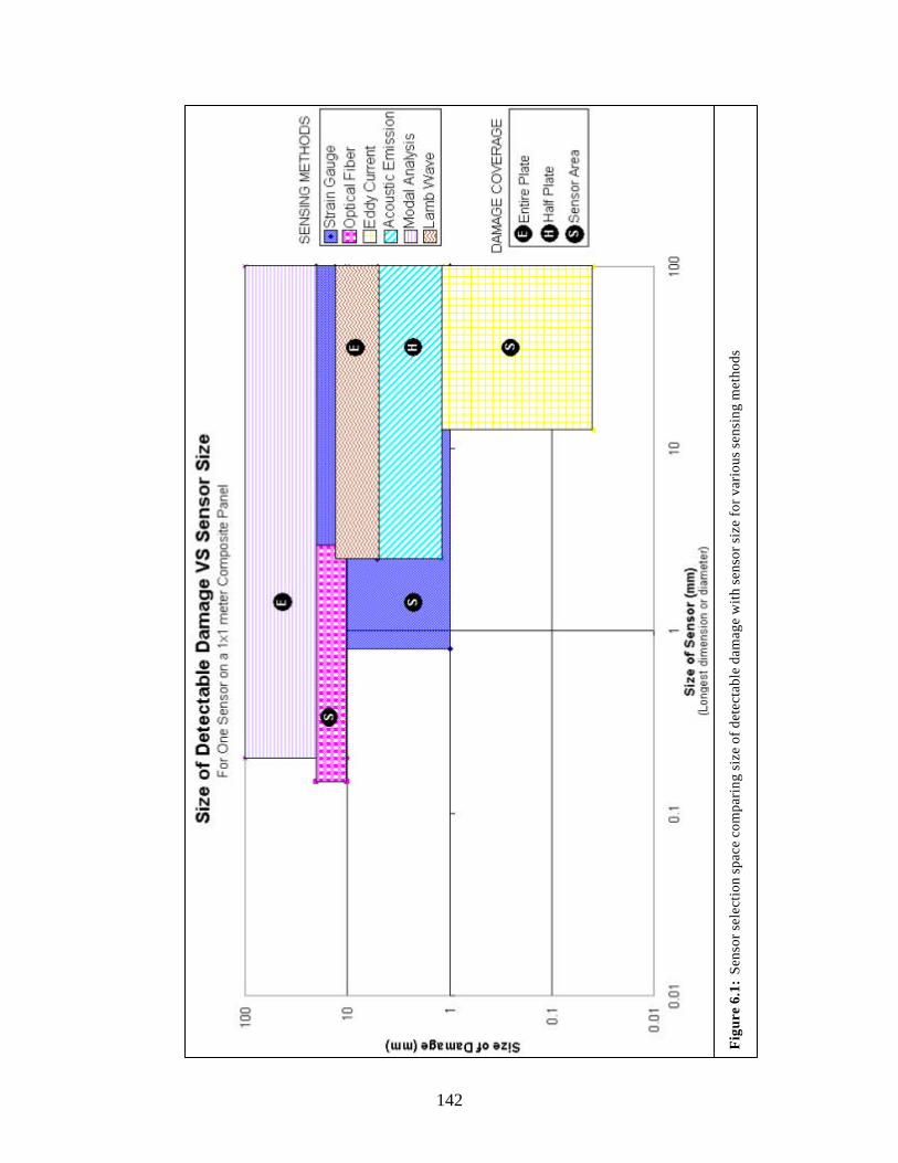
142
Fig
ure
6.1:
Sen
sor s
elec
tion
spac
e co
mpa
ring
siz
e of
det
ecta
ble
dam
age
with
sen
sor s
ize
for v
ario
us s
ensi
ng m
etho
ds

143
Fig
ure
6.2:
Sen
sor s
elec
tion
spac
e co
mpa
ring
siz
e of
det
ecta
ble
dam
age
with
sen
sor p
ower
for v
ario
us s
ensi
ng m
etho
ds

144
Method Strengths Limitations SHM Potential Visual Inexpensive equipment
Inexpensive to implement No data analysis Portable Simple procedure
Only surface damage Only large damage Human interpretation Can be time consuming
Currently none
X-radiography Penetrates surface Small defects with penetrant No data analysis Permanent record of results Simple procedure
Expensive equipment Expensive to implement Human interpretation Can be time consuming Require access to both sides Safety hazard
Currently none
Strain gauge Portable Embeddable Surface mountable Simple procedure Low data rates
Expensive equipment Expensive to implement Data analysis required Localized results
Lightweight Conformable Can be deposited Very low power draw Results for small area
Optical fibers Inexpensive equipment Embeddable Quick scan of large area
Expensive to implement Data analysis required High data rates Accuracy in question
Lightweight Large area coverage Must be embedded Requires laser
Ultrasonic Inexpensive to implement Portable Sensitive to small damage Quick scan of large area
Very expensive equipment Complex results Specialized software High data rates Couplant required Require access to both sides
Currently none
Eddy current Inexpensive to implement Portable Surface mountable Sensitive to small damage
Expensive equipment Very complex results Specialized software Safety hazard Conductive material only
Lightweight Conformable Can be deposited Very high power draw Results for small area
Acoustic emission Inexpensive equipment Inexpensive to implement Surface mountable Portable Quick scan of large area Sensitive to small events
Very complex results Very high data rates Specialized software
Lightweight Conformable Can be deposited No power required Results for large area Triangulation capable
Modal analysis Inexpensive equipment Inexpensive to implement Surface mountable Portable Simple procedure Quick scan of large area
Complex results High data rates Specialized software Results are global
Lightweight Conformable Can be deposited Multi-purpose sensors Low power required Results for large area
Lamb waves Inexpensive equipment Inexpensive to implement Surface mountable Portable Sensitive to small damage Quick scan of linear space
Very complex results Very high data rates Specialized software
Lightweight Conformable Can be deposited Medium power draw Linear scan results Triangulation possible
Table 6.1: Comparison of strengths, limitations and SHM implementation potential for various sensing systems

145
Chapter 7
CONCLUSIONS AND RECOMMENDATIONS
The previous chapters of this thesis have demonstrated the ability of piezoelectric sensors
to detect damage in composite materials by various methods. Motivations for the application of
structural health monitoring, its component requirements and the current state of SHM in
industry have also been provided. This chapter draws conclusions from the analytical and
experimental work presented in this thesis, and presents recommendations for further
experimentation in this field. The following is a list of key contributions provided in this thesis,
along with a summary of the other analytical and experimental results presented herein:
Key Contributions
• This thesis provides a thorough optimization study for the selection of Lamb wave propagation parameters. These include the choice of driving frequency, pulse shape, actuator geometry and sensor spacing. Signal decomposition and noise reduction are also discussed. The presented approach can be used to apply Lamb wave methods to detect damage in composite or metallic structures alike. A complete collection of these formulations is non-existent in the literature. (Section 4.3)
• An argument is presented using the finite element results for the modal analysis method that
demonstrates the dependence of the frequency response of a structure on the damage type, location and orientation. Various combinations of damage would yield identical frequency shifts (or damage signatures), making model-dependent modal analysis methods impractical for SHM applications. (Section 3.5.1)
• A cohesive description of SHM components and their requirements is presented, currently not
found in a single published paper in the literature. An SHM system architecture is proposed for implementation within a composite structure, with recommendations based upon the analytical and experimental results from this thesis. (Section 6)

146
Analytical Results • Full Lamb wave derivation and solution for phase and group velocities commencing from
original Lamb papers, which can be used to as a reference to replace many incorrect formulations in the literature. (Section 4.2.1)
• Direct comparison of damage sensitivities in identical finite element models solved by
frequency response and Lamb wave techniques. (Section 4.6.2) Experimental Results • Frequency response experimental results presented for comparison with a much larger range
of representative damage types in specimens than anywhere else in the literature. (Section 3.4.2)
• Detailed description of Lamb wave test setup, with explanations for parameter calculations.
Mostly non-existent or arbitrary in literature. (Section 4.3) • First published work to document experimental Lamb wave results for specimens with damage
other than delamination, including matrix cracks, fiber fracture and through-holes. (Section 4.5.2)
• First published work to document experimental Lamb wave results for complex composite
geometries. Results presented for 1-D application of Lamb wave tests in composite built up structure such as sandwich beams with various cores, rib-stiffened panels and a sandwich construction cylinder. New configurations of 2-D plate tests were also performed for Lamb wave techniques. (Section 4.5.2)
• Preliminary testing of acoustic emission methods and strain monitoring techniques for
application in SHM system with frequency response and Lamb wave sensors. (Section 5.2) General Results • Economic and reliability motivations for SHM applications presented. (Section 2.3.1) • Description of strengths, weaknesses, limitations and SHM applicability for frequency
response and Lamb wave methods. Suggested roles for these methods within a SHM system. (Section 4.6.3)
• Thorough review paper of current SHM systems, and available components (Section 2.3.2)

147
7.1 Conclusions
This thesis presented an analytical and experimental study of various piezoelectric-based
in-situ damage detection techniques as a basis for the health monitoring of composite materials.
The main focus was placed on frequency response methods, which have traditionally received
the most attention, and Lamb wave methods, which are now being heavily researched as having
the most potential for damage detection in composite applications. For each of these methods, a
thorough literature review was presented, followed by an analytical study to predict the
theoretical sensitivity of each of these methods to representative damage. These studies were
supported by finite element solutions for identical models using each method for comparison.
Finally, each method was tested experimentally using a single set of specimens with several
forms of representative damage. The strengths, weakness, and limitations of each method were
explained and compared, and suggestions for implementation of these methods into a SHM
system were given.
Using frequency response methods, good correlation was found between the model and
the experimental results for low frequencies, however coalescing modes at higher frequencies
made comparison impractical. In both the finite element models and experimental results there
was strong correspondence between the extent of damaged and reduction in natural frequencies.
Frequency response methods appear to be appropriate for detecting global changes in stiffness,
for relatively large structures at a low power, or possibly even using ambient vibration energy.
Not much information about the specifics of location or type of damage can be inferred by this
method however, without the use of large stored models. Frequency response methods have a
potentially useful role in a SHM system, by guiding other active sensor systems to regions of
concern and monitoring the global decay of structural stiffness.

148
Using the models created for the frequency response methods, a finite element analysis
was also performed for Lamb wave techniques. Lamb wave times of flight measurements were
taken from the animations for comparison with experimental results. These experiments were
setup using a series of optimization tools created using mathematical models developed and
combined as a part of this thesis, and were performed on the narrow coupons from the previous
frequency response tests. Similar tests were also performed on sandwich beams using cores of
various densities and stiffness, plates with rib-stiffeners, 2-D plates and a composite micro-
satellite. These tests demonstrated the feasibility of detecting several types of flaws in
representative composite structures. The experimental procedure used in this thesis was also
validated successfully by a “blind test” of several beam specimens. Lamb wave techniques have
the potential to provide more information than frequency response methods since they are more
sensitive to the local effects of damage to a material than the global response of a structure. The
disadvantage of these methods is that they require an active driving mechanism to propagate the
waves, however, Lamb wave methods have been found to be the most effective for the
determination of the presence of damage in composite materials.
Furthermore this thesis described each component integral to a SHM system. This
includes the sensors, processors, communication and power systems, algorithms, intervention
systems and the architecture that binds them all together. A recommendation was provided for a
feasible architecture for current implementation, and a prediction for the future of SHM systems
is given. Structural heath monitoring systems are likely to be an important component in future
designs of composite air and spacecraft to increase the feasibility of their missions and reduce
their life-cycle costs, and in-situ piezoelectric-based NDE techniques will likely play a role in
these systems.

149
7.2 Recommendations for Future Work
Much work still remains before current SHM systems can be relied upon to replace
standard inspection and maintenance cycles. For frequency response methods, more experiments
should be performed on built-up and larger structures to confirm the initial results. An
experiment study paralleling the performed tests but varying the size of the damaged regions
would also be useful in determining this method’s sensitivity. For Lamb wave testing, further
work lies ahead for different types of built-up structures other than the ones tested during the
present research, including joined sections and tapers in laminate thickness. A more thorough
investigation of 2-D sensing is necessary, as well as further investigation into the potential
capabilities of “self-sensing” actuators. It would also be interesting to perform more experiments
using one set of sensors to perform several types of tests, which should also be implemented on
representative structures in future testing. Another possibility would be to test these methods on
materials in use, since the present work only included newly manufactured specimens with
artificially introduced damage, and did not account for the complexities inherent to retrofitting a
system to an aging structure.
Beyond the methods examined in this thesis, there are also other useful methods that
should be explored using similar procedures. This includes eddy current measurement, and
several other electrical and magnetic impedance measurement methods. Another avenue of
research could be pursuing all of the previously mentioned methods using new types of sensors,
designed to be lightweight and conformable specifically for SHM applications. After good
sensors and sensing systems have been developed, much work still remains on each of the other
components of SHM systems. Testing the integration of these components will be an important

150
part of a successful program. Most directly, remotely controlling and accessing data from
sensors via wireless connection and power still needs much attention. There are many
components that have yet to be suitably developed for SHM applications, however the aerospace
community has a present understanding of the need for SHM systems, and they will be a reality
in the near future.

151
REFERENCES
1. Hall S.R. “The Effective Management and Use of Structural Health Data.” Proceedings of the 2nd International Workshop on Structural Health Monitoring, 1999, 265-275.
2. Hall S.R. and T.J. Conquest. “The Total Data Integrity Initiative—Structural Health Monitoring, The Next Generation.” Proceedings of the USAF ASIP, 1999. 2nd ed.
3. Bhat. N. “Delamination Growth in Graphite/Epoxy Composite Laminates Under Tensile Load.” Massachusetts Institute of Technology, Cambridge, Ma, USA. 1993.
4. Wang S.S. “Delamination Crack Growth in Unidirectional Fiber-Reinforced Laminates under Static and Cyclic Loading.” Composite Material: Testing and Design, ASTM STP (674), 1979, 642-663.
5. Bar-Cohen Y. “Emerging NDE Technologies and Challenges at the Beginning of the 3rd Millennium.” Materials Evaluation, 1999.
6. Khan M.A.U. “Non-destructive Testing Applications in Commercial Aircraft Maintenance.” Proceedings of the 7th European Conference on Non-Destructive Testing, v.4, 1999.
7. Chang FK. “Structural Health Monitoring: A Summary Report.” Proceedings of the 2nd International Workshop on Structural Health Monitoring, Stanford, CA, September 8-10, 1999.
8. Oka K., Ohino H., Kurashima T., Matsumoto M., Kumagai H., Mita A. and K. Sekijima. “Fiber Optic Distributed Sensor for Structural Monitoring.” Proceedings of the 2nd International Workshop on Structural Health Monitoring, 1999, 672-679.
9. Rogers A. “Distributed Optical-Fibre Sensing.” Measurement Science and Technology, v.10, 1999, 75-99. Kim K.S., Kollar L. and G.S. Springer. “A Model of Embedded Fiber Optic Fabry-Perot Temperature and Strain Sensors.” Journal of Composite Materials, v.27, 1993, 1618-1661.
10. Kollar L. and R.J. Steenkiste. “Calculation of the Stresses and Strains in Embedded Fiber Optic Sensors.” Journal of Composite Materials, v.32, 1998, 1647-1679.
11. Todd M.D., Johnson G.A., Althouse B.A. and S.T. Vohra. “Flexural Beam-Based Fiber Bragg Grating Accelerometers.” IEEE Photonics Technology Letters, v.10, 1998, 1605-1607
12. Parker T.R., Farhadiroushan M., Feced R. and V.A. Handerek. “Simultaneous Distributed Measurement of Strain and Temperature form Noise-Initiated Brillouin Scattering in Optical Fibers.” IEEE Journal of Quantum Electronics, v.34, 1998, 645-659.
13. Kim K.S., Ismail Y. and G.S. Springer. “Measurement of Strain and Temperature with Embedded Intrinsic Fabry-Perot Optical Fiber Sensors.” Journal of Composite Materials, v.27, 1993, 1663-1677.
14. Soloman S. Sensors Handbook. McGraw-Hill, New York, NY, 1998. 15. Bocherens E., Bourasseau S., Dewynter-Marty V., Py S., Dupont M., Ferdinand P. and H.
Berenger. “Damage Detection in a Radome Sandwich Material with Embedded Fiber Optic Sensors.” Smart Materials and Structures, v.9, 2000, 310-315.
16. Green A.K., Zaidman M., Shafir E., Tur M. and S. Gali. “Infrastructure Development for Incorporation Fibre-Optic Sensors in Composite Materials.” Smart Materials and Structures, v.9, 2000, 316-321.
17. Steenkiste R.J., and L. Kollar. “Effect of Coating on the Stresses and Strains in an Embedded Fiber Optic Sensor.” Journal of Composite Materials, v.32, 1998, 1680-1711.

152
18. Goldfine N., Schlicker D. and A. Washabaugh. “Surface-Mounted Eddy-Current Sensors for On-Line Monitoring of Fatigue Tests and for Aircraft Health Monitoring.” Proceedings of the 2nd Joint NASA/FAA/DoD Conference on Aging Aircraft, 1998.
19. Goldfine N., Washbaugh A. and K. Walrath. “Conformable Eddy Current Sensors and Methods for Gas Turbine Inspection and Health Monitoring.” Gas Turbine Materials Technology, 1999, 105-114.
20. Goldfine N. and V. Zilberstein. “Recent Applications of Meandering Winding Magnetometers to Materials Characterization.” Insight: Non-Destructive Testing and Condition Monitoring, v.42, 2000, 154-165.
21. Goldfine N., Washbaugh A. and D. Schlicker. “High Resolutoin Inductive Array Imaging of Buried Objects.” SPIE AeroSense 2000, Orlando, FL, April 2000.
22. Yentzer T., Zolberstein V., Goldfine N., Schlicker D. and D. Clark. “Anisotropic Conductivity Measurements for Quality Control of C-130/P-3 Propeller Blades Using MWM-Sensors with Grid Methods.” Proceedings of the 4nd Joint NASA/FAA/DoD Conference on Aging Aircraft, 2000.
23. Goldfine N., Washbaugh A., Schlicker D., and V. Zilberstein. “Application of MWM-Array Eddy Current Sensor to Corrosion Mapping.” Proceedings of 4th International Aircraft Corrosion Workshop, August 2000.
24. Mamishev A.V., Lesieutre B.C., and M. Zahn. “Optimization of Multi-Wavelength Interdigital Dielectrometry Instrumentation and Algorithms.” IEEE Transactions on Dielectrics and Electrical Insulation, v.5, 1998, 408-420.
25. Zahn M. “Optical, Electrical and Electromechanical Measurement Methodologies of Fields, Charge and Polarization in Dielectrics.” IEEE Transactions on Dielectrics and Electrical Insulation, v.5, 1998, 627-650.
26. Dowell M. and G. Sylvester. “Turbomachinery Prognostics and Health Management via Eddy Current Sensing: Current Developments.” General Dynamics Report, 2000.
27. Aberg M. and P. Gudmundson. “Micromechanical Modeling of Transient Waves from Matrix Cracking and Fiber Fracture in Laminated Beams.” International Journal of Solids and Structures, v.37, 2000, 4083-4102.
28. Zheng G.T., Buckley M.A., Kister G. and G.F. Fernando. “Blind Deconvolution of Acoustic Emission Signals for Damage Identification in Composites.” AIAA Journal, v.39, 2001, 1198-1205.
29. Marantidis C., Van Way C.B. and J.N. Kudva. “Acoustic-Emission Sensing in an On-Board Smart Structural Health Monitoring System for Military Aircraft.” Proceedings of the SPIE Conference on Smart Structures and Integrated Systems, v. 2191, 1994, 258-264.
30. Schoess J.N. and J.D. Zook. “Test Results of Resonant Integrated Microbeam Sensor (RIMS) for Acoustic Emission Monitoring.” Proceedings of the SPIE Conference on Smart Electronics and MEMS, v.3328, 1998, 326-332.
31. Menon S. and J.N. Schoess. “Stress Wave Acoustics Analysis for the CH-46 Sea Knight Rotor System.” Honeywell Technology Center Report, 1999.
32. Schoess J.N. “Development and Application of Stress-Wave Acoustic Diagnostics for Roller Bearings.” Honeywell Technology Center Report, 1999.
33. Giurgiutiu V., Bao J. and W. Zhao. “Active Sensor Wave Propagation Health Monitoring of Beam and Plate Structures.” Proceedings of the 8th International SPIE Symposium on Smart Structures and Materials, Newport Beach, CA, 2001.
153
34. Monkhouse R.S.C., Wilcox P.W., Lowe M.J.S., Dalton R.P., and P. Cawley. “The rapid Monitoring of Structures using Interdigital Lamb Wave Transducers.” Smart Materials and Structures, v.9, 2000, 304-309.
35. Todoroki A., Tanaka Y. and Y. Shimamura. “Response Surface for Delamination Monitoring of Gr/Ep Composites Using Electric Resistance Change.” Proceedings of the International Workshop on Structural Health Monitoring, 1999, 308-316.
36. Thompson L. and B. Westermo. “A New Strain Measurement Technology for Material Damage Assessment.” Proceedings of the SPIE Conference on Smart Structures, v.2191, 1996, 380-391.
37. Monaco E., Franco F. and L. Lecce. “Structural Damage Identification using Magnetostrictive Actuators.” Proceedings of the SPIE Conference on Smart Structures and Integrated Systems, v. 3668, 1999, 395-404.
38. Jain M.K., Schmidt S. and Ong K.G.. “Magnetoacoustic Remote Query Temperature and Humidity Sensors.” Smart Materials and Structures, v.9, 2000, 502-510.
39. Emmerich H. and M. Schofthaler. “Magnetic Field Measurements with a Novel Surface Micromachined Magnetic-Field Sensor.” IEEE Transactions on Electron Devices, v.47, 2000, 972-977.
40. Baglio S., Latorre L. and P. Nouet. “Development of Novel Magnetic Field Monolithic Sensors with Standard CMOS Compatible MEMS Technology.” Proceedings of the SPIE Conference on Smart Structures and Integrated Systems, v. 3668, 1999, 417-424.
41. Sage I., Badcock R., Humberstone L., Geddes N., Kemp M. and G. Bourhill. “Triboluminescent Damage Sensors.” Smart Materials and Structures, v.8, 1999, 504-510.
42. Javidinejad A. and S.P. Joshi. “Design and Structural Testing of Smart Composite Structures with Embedded Conductive Thermoplastic Film.” Smart Materials and Structures, v.8, 1999, 585-590.
43. Tamiatto C., Krawczak P., Pabiot J. and F. Laurent. “Integrated Sensors for In-Service Health Monitoring of Glass/Resin Composites.” Journal of Advanced Materials, v.30, 1998, 32-37.
44. Thompson L. and B. Westermo. “A New Strain Measurement Technology for Material Damage Assesment.” Proceedings of the SPIE Conference on Smart Structures and Integrated Systems, v. 2191, 1994, 380-391.
45. Cao L., Kim T.S., Zhou J., Mantell S.C. and D.L. Polla. “Calibration Technique for MEMS Membrane Type Strain Sensors.” Proceedings of the IEEE, 1999, 204-210.
46. Banaszak D., Dale G.A., and A.N. Watkins. “An Optical Technique for Detecting Fatigue Cracks in Aerospace Structures.” Proceedings of the IEEE, 1999, 271-277.
47. http://www.faa.gov/avr/AFS/FARS/far-25.txt 48. http://www.airweb.faa.gov/Regulatory_and_Guidance_Library/rgAD.nsf/HomeFrame 49. Schmidt H.J., Schmidt-Bradecker B. and G. Tober. “Design of Modern Aircraft Structure
and the Role of NDI.” Proceedings of the 7th European Conference on Non-Destructive Testing, v.4, 1999.
50. Suresh S. Fatigue of Materials. 2nd Edition, Cambridge Press, 1998. 51. Amer KB. “A new philosophy of structural reliability, fail safe versus safe life,”
Proceedings of the 44th Annual Forum of the American Helicopter Society, 1988, 3-16. 52. Lee J, Harris B, Almond DP and F. Hammett. “Fibre Composite Fatigue-Life
Determination,” Composites Part A-Applied Science and Manufacturing, v.1, 1997, 5-15.
154
53. Nyman T. “Composite Fatigue Design Methodology: A Simplified Approach,” Composite Structures, v.2, 1996, 183-194.
54. Radhakrishnan VM. “Endurance Diagram,” International Journal of Fatigue, v.6, 1990, 513-517.
55. O’Brian TK. “Towards a Damage Tolerance Philosophy for Composite Materials and Structures,” Composite Materials: Testing and Design, v.9, 1990, 7-33.
56. Shokrieh MM and LB Lessard. “Residual Fatigue Life Simulation of Laminated Composites,” Proceedings of the International Conference on Advanced Composites, 1998, 79-86.
57. Michael J, Dickson B and T Cambell. “Analysis of Use of Damage Tolerance Criteria for Helicopter Design,” Proceedings of the 55th Annual Forum of the American Helicopter Society, v.2, 1999, 1219-1231.
58. Talreja R. “Damage Mechanics and Fatigue Life Assessment of Composite Materials,” International Journal of Damage Mechanics, v.8, 1999, 339-354.
59. http://www.faa.gov/avi/air/asc/20-107a.doc 60. Rouchon J. “Certification of Large Airplane Composite Structures.” ICAS Congress
Proceedings, v.2, 1990, 1439-1447. 61. Chaumette D. “Certification Problems for Composite Airplane Structures.” Proceedings of
the 6th International European SAMPE Conference. 1985, 19-28. 62. Smith PJ and RD Wilson “Damage Tolerant Composite Wing Panels for Transport
Aircraft.” NASA Technical Report CR-3951. 63. Ng K.W. “Integrated Diagnostics and Prognostics of Rotation Machinery.” Office of Naval
Research Report. 64. Bar-Cohen Y., Chang Z. and A. Mal. “Characterization of Defects in Composite Materials
using Rapidly Acquired Leaky Lamb Wave Dispersion Data.” Proceedings of the 7th European Conference on Non-Destructive Testing, v.3, 1998.
65. Wang J.M. “An Internet Based System to Monitor Aircraft’s Health.” S.M. thesis, Massachusetts Institute of Technology, June 2001.
66. Low, S. Jane’s All the World’s Aircrafts. 2001, 102-165. 67. Neumair M. “Requirements on Future Structural Health Monitoring Systems.” Proceedings
of the 7th RTO Meetings, May 1998. 68. Zimmerman D.C., Simmermacher T. and M. Kaouk. “Model Correlation and System
Health Monitoring using Frequency Domain Measurements.” AIAA Journal, 1995, 3318-3325.
69. Abdelghani M., Goursat M. and T. Biolchini. “On-Line Modal Monitoring of Aircraft Structures under Unknown Exication.” Mechanical Systems and Signal Processing, v.13, 1999, 839-853.
70. Dalton R.P., Cawley P. and M.J.S. Lowe. “The Potential of Guided Waves for Monitoring Large Areas of Metallic Aircraft Fuselage Structure.” Journal of Nondestructive Evaluation, v.20, 2001, 29-46.
71. Schoess J.N. “Distributed System Architecture Alternatives for Condition Based Maintenance (CBM).” Honeywell Technology Center Report, 1999.
72. Van Way C.B., Kudva J.N. and Schoess J.N. “Aircraft Structural Health Monitoring System Development—overview of the Air Force/Navy Smart Metallic Structures Program.” Proceedings of the SPIE Symposium on Smart Structures and Materials, San Diego, CA, 1995.

155
73. Goldfine N., Schlicker D. and A. Washabaugh. “Surface-Mounded Eddy-Current Sensors for On-Line Monitoring of Fatigue Tests and for Aircraft Health Monitoring.” Proceedings of the 2nd Joint NASA/FAA/DoD Conference on Aging Aircraft, 1998.
74. Zou Y., Tong L. and G.P. Steven. “Vibration-Based Model-Dependant Damage (Delamination) Identification and Health Monitoring for Composite Structures—A Review.” Journal of Sound and Vibration, v.2, 2000, 357-378.
75. Zhang H., Schulz M.J. and F. Feruson. “Structural Health Monitoring Using Transmittance Functions.” Mechanical Systems and Signal Processing, v.5, 1999, 765-787.
76. Dunne J.P., Pitt D.M. and D.A. Sofge. “Recent Advances in Active Damage Interrogation.” Proceedings of the 42nd AIAA SDM Conference, Seattle, WA, 2001.
77. Deng X., Wang Q. and V. Giugiutiu.” Proceedings of the 6th International SPIE Symposium on Smart Structures and Materials, Newport Beach, CA, 1999.
78. Lemistre M. and D. Balageas. “Structural Health Monitoring System based on Diffracted Lamb Wave Analysis by Multiresolution Processing.” Smart Materials and Structures, v.10, 2001, 504-511.
79. Wang X. and G. Huang. “Elastic Wave Propagation Induced by Piezoelectric Actuators for Health Monitoring of Structures.” Journal of Intelligent Material Systems and Structures, v.10, 1999.
80. Osmont D., Devillers D. and F. Taillade. “A Piezoelectric Based healther Monitoring System for Sandwich Plates Submitted to Damaging Impacts.” European Congress on Computational Methods in Applied Sciences and Engineering, 2000.
81. Valdez S.H.D. and C. Soutis. “A Structural Health Monitoring System for Laminated Composites.” Proceedings of the 18th Biennial Conference on Mechanical Vibration and Noise, 2001.
82. Valdez S.H.D. and C. Soutis. “Health Monitoring of Composites using Lamb Waves generated by Piezoelectric Devices.” Plastics, Rubber and Composites¸v.29, 2000, 475-481.
83. Bar-Cohen Y. “NDE of Fiber Reinforced Composite Materials—A Review.” Materials Evaluation, v.44, 1986, 446-454.
84. Doebling S.W., Farrar C.R., Prime M.B. and D.W. Shevitz. “Damage Identification and Health Monitoring of Structural and Mechanical Systems from Changes in their Vibration Characteristics: A Literature Review.” Los Alamos National Laboratory Technical Report, LA-13070-MS, 1996.
85. Gadelrab R.M. “The Effect of Delamination on the Natural Frequencies of a Laminated Composite Beam.” Journal of Sound and Vibration, v.197, 1996, 283-292.
86. Alampalli S. “Effects of Testing, Analysis, Damage, and Environment on Modal Parameter.” Mechanical Systems and Signal Processing, v.14, 2000, 63-74.
87. Cawley P. and R.D. Adams. “A Vibration Technique for Non-Destructive Testing of Fibre Composite Structures.” Journal of Composite Materials, v.13, 1979, 161-175.
88. Cawley P. and R.D. Adams. “The location of Defects in Structure form Measurements of Natural Frequencies.” Journal of Strain Analysis, v.14, 1979, 49-57.
89. Narayana K.L. and C. Jebaraj. “Sensitivity Analysis of Local/Global Modal Parameters for Identification of a Crack in a Beam.” Journal of Sound and Vibration, v.228, 1999, 977-994.
156
90. Parker B.E., Ware H.A., Wipf D.P., Tompkins W.R., Clark B.R., Larson E.C. and H.V. Poor “Fault Diagnostics using Statistical Changes in the Bispectral Domain.” Mechanical Systems and Signal Processing, v.14, 2000, 561-570.
91. Park K.C. and G.W. Reich. “Model-Based Health Monitoring of Structural Systems: Progress, Potential and Challenges.” .” Proceedings of the 2nd International Workshop on Structural Health Monitoring, 1999, 82-95.
92. Abdelghani M., Goursat M. and T. Biolchini. “On-Line Modal Monitoring of Aircraft Structures under Unknown Excitation.” Mechanical Systems and Signal Processing, v.13, 1999, 839-853.
93. Sampaio R.P.C., Maia N.M.M. and J.M.M. Silva. “Damage Detection using the Frequency-Response-Function Curvature Method.” Journal of Sound and Vibration, v.226, 1999, 1029-1042.
94. Chiu W.K., Galea S.C., Loss L.L. and N. Rajic. “Damage Detection in Bonded Repars using Piezoceramics.” Smart Materials and Structures, v.9, 2000, 466-475.
95. Bedewi N.E. and D.N. Kung. “Effect of Fatigue Loading on the Modal Properties of Composite Structures and its Utilization for Prediction of Residual Life.” Composite Structures, v.37, 1997, 357-371.
96. Valdes S.H.D. “Structural Integrity Monitoring of CFRP Laminates using Piezoelectric Devices.” Ph.D. thesis, Imperial College of Science Technology and Medicine, September 2000.
97. Kaouk M. and D.C. Zimmerman. “Structural Damage Detection Using Measured Modal Data and No Original Analytical Model.” Proceedings of the International Modal Analysis Conference, v.1, 1994, 731-737.
98. James G.H. and D.C. Zimmerman. “An Experimental Study of Frequency Response Function (FRF) Based Damage Assessment Tools.” Proceedings of the International Modal Analysis Conference, v.1, 1998, 151-157.
99. Zimmerman D.C., Simmermacher T. and M. Kaouk. “Structural Damage Detection Using Frequency Response Functions.” Proceedings of the International Modal Analysis Conference, v.1, 1995, 179-183.
100. Banks H.T. and P.R. Emeric. “Detection of Non-Symmetrical Damage in Smart Plate-Like Structures.” Journal of Intelligent Material Systems and Structures, v.9, 1998, 818-828.
101. Mitchell K., Sana S., Balakrishnan V.S., Rao V.S., and H.J. Pottinger. “Micro Sensors for Health Monitoring of Smart Structures.” Proceedings of the SPIE Conference on Smart Electronics and MEMS, v.3673, 1999, 351-358.
102. Purekar A.S. and D.J. Pines. “Detecting Damage in Non-Uniform Beams Using the Dereverberated Transfer Function Response.” Smart Materials & Structures, v.9, 2000, 429-444.
103. Valdes S.H.D. and C. Soutis. “Delamination Detection in Composite Laminates from Variations of their Modal Characteristics.” Journal of Sound and Vibration, v.1, 1999, 1-9.
104. Meirovitch L. Elements of Vibration Analysis. 2nd ed, McGraw-Hill, New York, NY, 1986. 105. Blevins R. Formulas for Natural Frequency and Mode Shape. Krieger Publishing
Company, Malabar FL, 1995. 106. Jones, R. M. Mechanics of Composite Materials. 2nd ed, Taylor & Francis, Blacksburg,
VA, 1999. 107. Bathe K.J., and E.L. Wilson. “Large Eigenvalue Problems in Dynamic Analysis.”
Proceedings of the ASCE, EM6, 1972, 1471-1485.

157
108. Whitney J. “Effective Elastic Constants of Bidirectional Laminates Containing Transverse Ply Cracks.” Journal of Composite Materials, v.34, 2000, 954-978.
109. Tong J., Guild F.J., Ogin S.L. and P.A. Smith. “On Matrix Crack Growth in Quasi-Isotropic Laminates.” Composite Science and Technology, v.57, 1997, 1527-1535.
110. Lagace P.A., Brewer J.C., and C. Varnerin. “TELAC Manufacturing Course Notes.” TELAC Report 88-4B, Massachusetts Institute of Technology, 1990.
111. Avitabile P. “Modal Space — In Our Own Little World.” SEM Experimental Techniques, 1998.
112. Viktorov I.A. Rayleigh and Lamb Waves, Physical Theory and Applications. Plenum Press, New York, 1967.
113. Nayfeh A.H. Wave Propagation in Layered Anisotropic Media with Applications to Composites. v.39, Elsevier, Amsterdam, 1995.
114. Lamb H. “On Waves in an Elastic Plate.” Proceedings of the Royal Society of London. Series A, Containing Papers of a Mathematical and Physical Character, v.93, n.651, 1917, 293-312.
115. Worlton D.C. “Experimental Confirmation of Lamb Waves at Megacycle Frequencies.” Journal of Applied Physics, v.32, 1961, 967-971.
116. Demer L.J. and L.H. Fentnor. “Lamb Wave Techniques in Nondestructive Testing.” International Journal of Nondestructive Testing, v.1, 1969, 251-283.
117. White R.M. “Surface Elastic Waves.” Proceedings of the IEEE, v.58, no.8, 1970. 118. Wenzel S.W. and R.M. White. “Silicon-Based Ultrasonic Lamb-Wave Multisensors.” IEEE
Solid-State Sensor and Actuator Workshop, 1988, 27-30. 119. Wenzel S.W. and R.M. White. “A Multisensor Employing an Ultrasonic Lamb-Wave
Oscillator.” IEEE Transactions on Electronic Devices, v.35 1988, 735-743. 120. Wenzel S.W., Martin B.A. and R.M. White. “Generalized Lamb-Wave Multisensor.”
Proceedings of the IEEE Ultrasonics Symposium, v.1, 1988, 563-567. 121. Grondel S., Assaad J., Delebarre C., Blanquet P. and e. Moulin “The Propagation of Lamb
Waves in Multilayered Plates: Phase-Velocity Measurement.” Measurement Science and Technology, v.10, 1999, 348-353.
122. Niethammer M. and L.J. Jacobs. “Time-Frequency Representation of Lamb Waves.” Journal of the Acoustic Society of America, v.109, 2001, 1841-1847.
123. Valle C., Niethammer M. and L.J. Jacobs. “Crack Characterization using Guided Circumferential Waves.” Journal of the Acoustic Society of America, v.110, 2001, 1282-1290.
124. Cho Y. “Lamb Wave Scattering Analysis for Reflector Characterization.” IEEE Transactions on Ultrasonics, Ferroelectrics, and Frequency Control, v.44, 1997, 44-52.
125. Pagneux V. and A. Maurel. “Determination of Lamb Mode Eigenvalues.” Journal of the Acoustic Society of America, v.110, 2001, 1307-1314.
126. Deutsch W.A.K. and K. Deutsch. “Defect Detection with Rayleigh and Lamb Waves Generated by a Self-Focusing Phased Array.” Proceedings of the 7th European Conference on Non-Destructive Testing, v.3, 1998.
127. Lee Y.C. “Measuring Lamb Wave Dispersion Curves of a Bi-Layered Plate and its Applications on Material Characterization of Coating.” IEEE Transactions on Ultrasonics, Ferroelectrics, and Frequency Control, v.48, 2001, 830-837.
128. Lee Y.C. “Measurements of Dispersion Curves Leaky Lamb Waves using a Lens-Less Line-Focus Transducer.” Ultrasonics, v.39, 2001, 297-306.
158
129. Lemistre M and D. Balageas. “Structural Health Monitoring System based on Diffracted Lamb Wave Analysis by Multiresolution Processing.” Smart Materials and Structures, v.10, 2001, 504-511.
130. Monkhouse R.S.C., Wilcox P.D. and P. Cawley. “Flexible Interdigital PVDF Transducers for the Generation of Lamb Waves in Structures.” Ultrasonics, v.35, 1997, 489-498.
131. Wilcox P., Lowe M., and P. Cawley. “Lamb and SH Wave Transducer Arrays for the Inspection of Large Areas of Thick Plates.” Proceedings of the 15th World Conference on Non-Destructive Testing, Rome, 2000.
132. Dalton R.P., Cawley P. and M.J.S. Lowe. “The potential of Guided Waves for Monitoring Large Areas of Metallic Aircraft Fuselage Structure.” Journal of Nondestructive Evaluation, v.20, 2001, 29-46.
133. Saravanos D.A. and P.R. Heyliger. “Coupled Layerwise Analysis of Composite Beans with Embedded Piezoelectric Sensors and Actuators.” Journal of Intelligent Material Systems and Structures, v.6, 1995, 350-362.
134. Saravanos D.A., Birman V. and D.A. Hopkins. “Detection of Delaminations in Composite Beams using Piezoelectric Sensors.” Proceedings of the 35th Structures, Structural Dynamics and Materials Conference of the AIAA, 1994.
135. Percival W.J. and E.A. Birt. “A Study of Lamb Wave Propagation in Carbon-Fibre Composites.” Insight: Non-Destructive Testing and Condition Monitoring, v.39, 1997, 728-735.
136. Birt E.A. “Damage Detection in Carbon-Fibre Composites using ultrasonic Lamb Waves.” Insight: Non-Destructive Testing and Condition Monitoring, v.40, 1998, 335-339.
137. Badcock R.A. and E.A.Birt “The use of 0-3 Piezocomposite Embedded Lamb Wave Sensors for Detection of Damage in Advanced Fibre Composites.” Smart Materials and Structures, v.9, 2000, 291-297.
138. Seale M.D., Smith B.T. and W.H. Prosser. “Lamb Wave Assessment of Fatigue and Thermal Damage in Composites.” Journal of the Acoustic Society of America, v.103, 1998, 2416-2424.
139. Tang B. and E.G. Henneke. “Lamb Wave Monitoring of Axial Stiffness Reduction of Laminated Composite Plates.” Materials Evaluation, v.47, 1989, 928-933.
140. Rose J.L., Hay T. and V.S. Agarwala. “Skin to Honeycomb Core Delamination Detection with Guided Waves.” 4th Joint DOD/FAA/NASA Conference on Aging Aircraft, 2000.
141. Kundu T., Potel C., and J.F. de Belleval. “Importance of Near Lamb Mode Imaging of Multilayered Composite Plates.” Ultrasonics, v.39, 2001, 283-290.
142. Ishak S.I., Liu G.R., Lim S.P. and H.M. Shang. “Experimental Study on Employing Flexural Wave Measurements to Characterize Delamination in Beams.” Experimental Mechanics, v.41, 2001 157-164.
143. Monnier T., Jayet Y., Guy P. and J.C. Baboux. “The Piezoelectric Implant Method: Implementation and Practical Applications.” Smart Materials and Structures, v.9 2000, 267-272.
144. Rose J.L. and T. Hay. “Skin to Honeycomb Core Delamination Detection with Guided Waves.” Proceedings of the 15th World Conference on Non-Destructive Testing, Rome, 2000.
145. Propser D. “Automated Detection of Wave Velocities in Concrete Bridge Decks.” PhD thesis, Massachusetts Institute of Technology, June 2001.

159
146. Fripp M. “Distributed Structural Actuation and Control with Electrostrictors.” SM thesis, Massachusetts Institute of Technology, June 1995.
147. Lively P. “Dynamic Structural Shape Estimation using Integral Sensor Arrays.” SM thesis, Massachusetts Institute of Technology, June 2000.
148. Strang G. and T. Nguyen Wavelets and Filter Banks. Wellesley-Cambridge Press, Wellesley, Ma, 1996.
149. “The Composite Materials Handbook MIL-17 Vol. 1” Guidelines for Characterization of Structural Materials.” MIL-HDBK-1E, Department of Defense, 1999.
150. Kessler S.S., Spearing S.M., Atalla M.J., Cesnik C.E.S. and C. Soutis. “Structural Health Monitoring in Composite Materials using Frequency Response Methods.” Proceedings of the SPIE International Symposium on Smart Strucutres and Material, 2001.
151. Lind R., Kyle S. and M. Brenner. “Wavelet Analysis to Characterize Non-Linearities and Predict Limit Cycles of an Aeroelastic System.” Mechanical Systems and Signal Processing, v.15, 2001, 337-356.
152. Dunn C. “The Analysis, Design, Manufacture, and Testing of a Composite Micro-Satellite.” SM thesis, Massachusetts Institute of Technology, February 2001.
153. Anderson E.H. “Piezoceramic Induced Strain Actuation of One and Two Dimensional Structures.” PhD thesis, Massachusetts Institute of Technology, June 1989.
154. Kollar L. and R.J. Steenkiste. “Calculation of the Stresses and Strains in Embedded Fiber Optic Sensors.” Journal of Composite Materials, v.32, 1998, 1647-1679.
155. Rees D., Chiu W.K. and R. Jones. “A Numerical Study of Crack Monitoring in Patched Structures using a Piezo Sensor.” Smart Materials and Structures, v.1, 1992, 202-205.
156. Chiu W.K., Galea S.C., Koss L.L. and N. Rajic. “Damage Detection in Bonded Repairs using Piezoceramics.” Smart Materials and Structures, v.9, 2000, 466-475.
157. Hautamaki C., Zurn S., Mantell S.C. and D.L. Polla. “Experimental Evaluation of MEMS Strain Sensors Embedded in Composites.” Journal of Microelectromechanical Systems, v.8, 1999, 272-279.
158. Sung D.U., Kim C.G. and C.S. Hong. “Simultaneous Monitoring of Impact Locations and Damages in Composite Laminates using Piezoceramics Sensors.” Proceedings of the 13th ICCM, Beijing, 2001.
159. Benmadakhene S. and A. Laksimi. “Propagation Study of Acoustic Emission Waves in Composite Materials.” Proceedings of the 13th ICCM, Beijing, 2001.
160. Aberg M. and P. Gudmundson. “Micromechanical Modeling of Transient Waves from Matrix Cracking and Fiber Fracture in Laminated Beams.” International Journal of Solids and Structures, v.37, 2000, 4083-4102.
161. Seydel R.E. and F.K. Chang. “Implementation of a Real-Time Impact Identification Technique for Stiffened Composite Panels.” Proceedings of the 2nd International Workshop on Structural Health Monitoring, 1999, 225-233.
162. Noonan E.E., Protz C.S., Peles Y.P. and S.M. Spearing. "Structural Analysis of a Micro-Rocket Combustion Chamber." Materials Research Society, November 2001, Boston, MA.
163. Ikegami R. “Structural Health Monitoring: Assessment of Aircraft Customer Needs.” Proceedings of the International Workshop on Structural Health Monitoring, 1999, 12-23.
164. Huber J.E., Fleck N.A. and M.F. Ashby. “The Selection of Mechanical Actuators based on Performance Indices.” Proceedings of the Royal Society of London, 1997, 2185-2205.
165. Horn D. and W.R. Mayo. “NDE Reliability Gains from Combining Eddy-Current and Ultrasonic Testing.” NDT&E International, v.33, 2000, 351-362.
160
166. Schoess J.N., Arch D. and Yang W. “MEMS Sensing and Control: An Aerospace Perspective.” Honeywell Technology Center Report, 2000.
167. Luginbuhl P., Collins S.D., Racine G.A., Gretillat M.A., de Rooij N.F., Brooks, K.G. and N. Setter. “Ultrasonic Flexural Lamb-Wave Actuators based on PZT Thin Film.” Sensors and Actuators A, v.64, 1998, 41-49.
168. Yuan L., Sana S., Pottinger H.J. and V.S. Rao. “Distributed Arithmetic Implementation of Multivariable Controllers for Smart Structural Systems.” Smart Materials and Structures, v.9, 2000, 401-412.
169. Pradhan S.S. and K. Ramchandran. “Distributed Source Coding: Symmetric Rates and Applications to Sensor Networks.” Proceedings of the IEEE, 2000, 363-372.
170. Das N.K., Khorrami F. and S. Nourbakhsh. “A New Integrated Piezoelectric-Dielectric Microstrip Antenna for Dual Wireless Actuation and Sensing Functions.” Proceedings of the SPIE Symposium on Smart Electronics and MEMS, San Diego, CA, 1998.
171. Porret A.S., Melly T., Enz C.C. and E.A. Vittoz. “Design of Hih-Q Varactors for Low-Power Wireless Applications using a Standard CMOS Process.” IEEE Journal of Solid-State Circuits, v.35, 2000, 337-345.
172. van den Boom T., Tebmann D., Lerch R., vom Boegel G., Hammerschmidt D., Amelung J., Hosticka B. and P. Mahdavi. “Romote CMOS Pressure Sensor Chip with Wireless Power and Data Transmission.” Proceedings of the IEEE International Solid-State Circuits Conference, 2000, 186-187.
173. Rabaey J., Ammer J., da Silva J.L. and D. Patel. “Ad-hoc Wireless Networking of Ubiquitous Low-Energy Sensor/Monitor Nodes.” Proceedings of the IEEE, 2000, 9-12.
174. Britton C.L., Warmack R.J., Smigh S.F., Oden P.I. and G.M. Brown. “MEMS Sensors and Wireless Telemetry for Distributed Systems.” Proceedings of the SPIE Symposium on Smart Electronics and MEMS, San Diego, CA, 1998.
175. Britton C.L., Warmack R.J., Smigh S.F., Oden P.I. and G.M. Brown. “Battery-Powered, Wireless MEMS Sensors for High-Sensitivity Chemical and Biological Sensing.” Proceedings of the IEEE, 1999, 359-368 .
176. Krantz D., Belk J., Dubow J., Hautamaki C., Matell S., Polla D. and S. Zurn. “Applied Research in Remotely-Queried Embedded Microsensors.” Proceedings of the SPIE Symposium on Smart Electronics and MEMS, San Diego, CA, 1998.
177. Varadan V.K., Teo P.T., Jose K.A. and V.V. Varadan. “Design and Development of a Smart Wireless System for Passive Temperature Sensors.” Smart Materials and Structures, v.9, 2000, 379-388.
178. Mitchell K., Sana S., Valakrishnan V.S., Rao V.S. and H.J. Pottinger. “Micro Sensors for Health Monitoring of Smart Structure.” Proceedings of the SPIE Symposium on Smart Electronics and MEMS, Newport Beach, CA, 1999.
179. Gilbert R.W., Bond L.J. and Skorpik J.R. “Smart Multi-Sensor Radio Frequency Tags for Propulsion Systems.” Pacific Northwest National Laboratory Report, 2000.
180. Pulitzer S.W. “Feasibility Assessment and Design of Micro Hydraulic Solid State Transducers.” S.M. thesis, Massachusetts Institute of Technology, June 1998.
181. Spillman W.B. and S. Durkee. “Non-Contact Power/Interrogation System for Smart Stuctures.” Proceedings of the SPIE Symposium on Smart Structures and Materials, San Diego, CA, 1994.
182. Bleay S.M, Loader C.B., Hawyes V.J., Humberstone L. and P.T. Curtis. “A smart Repair System for Polymer Matrix Composites.” Composites Part A, v.32, 2001, 1767-1776.
161
APPENDIX A
Mathematica Code for Phase and Group Velocities

162
(* CLPT code to determine material properties for laminate*) layup={90, 45, -45, 0}; sym=1; El=21500000*6912; Et=1460000*6912; vlt=.3; vtl=Et/El*vlt; G=810000*6912; t=.005*.0254; rho=.055*27680; ply=Length[layup]; q=IdentityMatrix[3]*0; q[[1,1]]=El/(1-vlt*vtl); q[[2,2]]=Et/(1-vlt*vtl); q[[1,2]]=(Et*vlt)/(1-vlt*vtl); q[[2,1]]=q[[1,2]]; q[[3,3]]=G; QBAR=IdentityMatrix[3]*0; For[z=1,z<=ply,z++, x=layup[[z]]*\[Pi]/180; a={{Cos[x]*Cos[x],Sin[x]*Sin[x],Cos[x]*Sin[x]},{Sin[x]*Sin[x], Cos[x]*Cos[x],-Cos[x]*Sin[x]},{-2*Cos[x]*Sin[x],2*Cos[x]*Sin[x], Cos[x]*Cos[x]-Sin[x]*Sin[x]}}; b=Transpose[a]; Q=b.q.a; QBAR=QBAR+Q;] QBAR=2*QBAR; A=QBAR/ply/2; As=Inverse[A]; Es11=As[[1,1]]; Es22=As[[2,2]]; Es33=As[[3,3]]; Es12=As[[1,2]]; E11=Es11^-1; E22=Es22^-1; G=Es33^-1; v=-Es12*E11; t=ply*2*t; (*Compute phase velocity*) n=0; x=Table[{j,j},{j,1,3000}]*0;
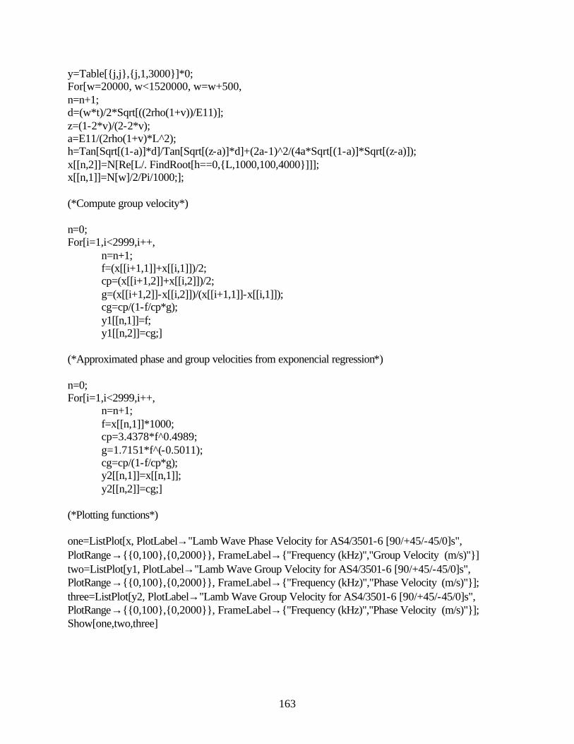
163
y=Table[{j,j},{j,1,3000}]*0; For[w=20000, w<1520000, w=w+500, n=n+1; d=(w*t)/2*Sqrt[((2rho(1+v))/E11)]; z=(1-2*v)/(2-2*v); a=E11/(2rho(1+v)*L^2); h=Tan[Sqrt[(1-a)]*d]/Tan[Sqrt[(z-a)]*d]+(2a-1)^2/(4a*Sqrt[(1-a)]*Sqrt[(z-a)]); x[[n,2]]=N[Re[L/. FindRoot[h==0,{L,1000,100,4000}]]]; x[[n,1]]=N[w]/2/Pi/1000;]; (*Compute group velocity*) n=0; For[i=1,i<2999,i++, n=n+1; f=(x[[i+1,1]]+x[[i,1]])/2; cp=(x[[i+1,2]]+x[[i,2]])/2; g=(x[[i+1,2]]-x[[i,2]])/(x[[i+1,1]]-x[[i,1]]); cg=cp/(1-f/cp*g); y1[[n,1]]=f; y1[[n,2]]=cg;] (*Approximated phase and group velocities from exponencial regression*) n=0; For[i=1,i<2999,i++, n=n+1; f=x[[n,1]]*1000; cp=3.4378*f^0.4989; g=1.7151*f^(-0.5011); cg=cp/(1-f/cp*g); y2[[n,1]]=x[[n,1]]; y2[[n,2]]=cg;] (*Plotting functions*) one=ListPlot[x, PlotLabel→"Lamb Wave Phase Velocity for AS4/3501-6 [90/+45/-45/0]s", PlotRange→{{0,100},{0,2000}}, FrameLabel→{"Frequency (kHz)","Group Velocity (m/s)"}] two=ListPlot[y1, PlotLabel→"Lamb Wave Group Velocity for AS4/3501-6 [90/+45/-45/0]s", PlotRange→{{0,100},{0,2000}}, FrameLabel→{"Frequency (kHz)","Phase Velocity (m/s)"}]; three=ListPlot[y2, PlotLabel→"Lamb Wave Group Velocity for AS4/3501-6 [90/+45/-45/0]s", PlotRange→{{0,100},{0,2000}}, FrameLabel→{"Frequency (kHz)","Phase Velocity (m/s)"}]; Show[one,two,three]

164
APPENDIX B
Lamb Wave Derivations
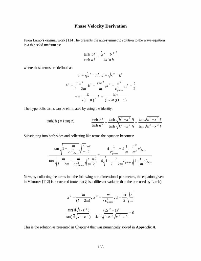
165
Phase Velocity Derivation From Lamb’s original work [114], he presents the anti-symmetric solution to the wave equation in a thin solid medium as: where these terms are defined as: The hyperbolic terms can be eliminated by using the identity: Substituting into both sides and collecting like terms the equation becomes: Now, by collecting the terms into the following non-dimensional parameters, the equation given in Viktorov [112] is recovered (note that ξ is a different variable than the one used by Lamb): This is the solution as presented in Chapter 4 that was numerically solved in Appendix A.
( )αβξβξ
αβ
2
222
4tanhtanh +=
ff
2222 , kh −=−= ξβξα
2,,,
2 2
22
22
22 t
fc
khphase
===+
=ω
ξµ
ρωµλ
ρω
))(12-(1E
, )2(1
Eνν
νλ
νµ
+=
+=
µρω
ρµ
ζµλ
µξ
2d , ,
)2( 222 t
c phase
==+
=
fk
fh
fik
fihff
22
22
22
22
tan
tan
tanh
tanhtanhtanh
ξ
ξ
ξ
ξαβ
−
−=
−
−=)tan()tanh( ziiz =
0--14
)12(
)-dtan(
)-1dtan(2222
22
22
2
=−
+ζξζζ
ζ
ζξ
ζ
22
22
2
2
2
2
12
14
14
14
22tan
21tan
phasephase
phasephase
phase
phase
cc
cc
tc
tc
µρ
µλρ
µρ
µ
ωµρ
ρµ
µλµ
ωµρ
ρµ
−+
−
+−=
−+
−

166
Group Velocity Derivation The group velocity of a traveling elastic wave is defined as: where the wavenumber k is defined as: Direct differentiation of this equality with respect to k yields the classical form: Alternatively, a more practical form can be reached by differentiating with respect to ω: This equation, which relies only on the frequency and phase velocity (which is also a function of frequency), can be implemented as part as a numerical solution as seen in Appendix A, or can be used to solve for the group velocity directly if the phase velocity equation is exponentially regressed (approximately a square root relationship) for a range of frequencies.
kk
ccc phase
phasegroup ∂∂
+=
kcgroup ∂
∂=
ω
phaseck
ω=
ωω
∂∂
⋅−=
phase
phase
phasegroup c
c
cc
1

167
Optimal Actuator Size Derivation The out of plane displacement of an elastic wave traveling in a solid medium follows the proportionality: where 2a is the length of the actuator in the direction of propagation. The maximum displacement is achieved were the derivative is zero: for which the solution is: manipulating this equality yields: where the wavenumber k is defined again as: Substituting this into the previous equality yields the practical form of this equation: where f is the frequency in Hertz. From this equation, the actuator dimensions can be optimized as discussed in Chapter 4.
kaW sin∝
0cos =kaa
0,1,2...nfor 2
)12( =+=π
nka
kna
π2)
21
(2 +=
phasephase cf
ck πω 2==
0,1,2...nfor )21
(2 =+=f
cna phase
168
APPENDIX C
ABAQUS Codes for Frequency Response and Lamb Wave Models

169
*HEADING Control Model for Frequency Response *NODE 1,0,0,0 8,0,0.7,0 21,0,2,0 211,1,0,0 218,1,0.7,0 231,1,2,0 841,4,0,0 848,4,0.7,0 861,4,2,0 1261,6,0,0 1268,6,0.7,0 1281,6,2,0 2101,10,0,0 2108,10,0.7,0 2121,10,2,0 *NGEN, NSET=N1 1,8,1 *NGEN,NSET=N2 8,21,1 *NGEN,NSET=N3 211,218,1 *NGEN,NSET=N4 218,231,1 *NGEN,NSET=N5 841, 848, 1 *NGEN,NSET=N6 848, 861, 1 *NGEN,NSET=N7 1261, 1268, 1 *NGEN,NSET=N8 1268, 1281, 1 *NGEN,NSET=N9 2101, 2108, 1 *NGEN,NSET=N10 2108, 2121, 1 *NFILL,NSET=CLAMPED1 N1, N3, 10, 21 *NFILL,NSET=CLAMPED2 N2, N4, 10, 21 *NFILL,NSET=BOTTOM1 N3, N5, 30, 21 *NFILL,NSET=BOTTOM2 N4, N6, 30, 21 *NFILL,NSET=DELAM N5, N7, 20, 21 *NFILL,NSET=UNDELAM N6, N8, 20, 21 *NFILL,NSET=TOP1 N7, N9, 40, 21 *NFILL,NSET=TOP2 N8, N10, 40, 21 *NSET,NSET=CLAMPED CLAMPED1,CLAMPED2

170
*NSET,NSET=UNDAMAGED BOTTOM1,BOTTOM2,TOP1,TOP2,UNDELAM,CLAMPED *NSET,NSET=ALL1 UNDAMAGED,DELAM *NCOPY,OLD SET=ALL1 ,CHANGE NUMBER=10000 ,NEW SET=ALL2 ,SHIFT 0,0,0.0 0,0,0,1,0,0,0 *MPC TIE,ALL2,ALL1 *ELEMENT,TYPE=S9R5 1,1,43,45,3,22,44,24,2,23 10001,10001,10043,10045,10003,10022,10044,10024,10002,10023 *ELGEN,ELSET=SPECIMEN1 1,10,2,1,50,42,10 *ELGEN,ELSET=SPECIMEN2 10001,10,2,1,50,42,10 *SHELL SECTION,OFFSET=SNEG,ELSET=SPECIMEN1,COMPOSITE .005,,LAMINA, 0. .005,,LAMINA,+45. .005,,LAMINA,-45. .005,,LAMINA, 90. *SHELL SECTION,OFFSET=SPOS,ELSET=SPECIMEN2,COMPOSITE .005,,LAMINA, 90. .005,,LAMINA,-45. .005,,LAMINA,+45. .005,,LAMINA, 0. **defined 90 degrees rotated *MATERIAL,NAME=LAMINA *ELASTIC,TYPE=LAMINA 21.5E6, 1.46E6, 0.3, 0.81E6, 0.46E6, 0.46E6 *DENSITY 0.0001417 *BOUNDARY CLAMPED, ENCASTRE *STEP, PERTURBATION *FREQUENCY, EIGENSOLVER=SUBSPACE 50, *RESTART,WRITE,OVERLAY *END STEP **-------

171
*HEADING Center Delamination Model for Frequency Response *NODE 1,0,0,0 21,0,2,0 211,1,0,0 231,1,2,0 946,4.5,0,0 966,4.5,2,0 1156,5.5,0,0 1176,5.5,2,0 2101,10,0,0 2121,10,2,0 *NGEN, NSET=N1 1,21,1 *NGEN,NSET=N2 211,231,1 *NGEN,NSET=N3 946, 966, 1 *NGEN,NSET=N4 1156, 1176, 1 *NGEN,NSET=N5 2101, 2121, 1 *NFILL,NSET=CLAMPED N1, N2, 10, 21 *NFILL,NSET=BOTTOM N2, N3, 35, 21 *NFILL,NSET=DELAM N3, N4, 10, 21 *NFILL,NSET=TOP N4, N5, 45, 21 *NSET,NSET=UNDAMAGED BOTTOM,TOP,CLAMPED *NCOPY,OLD SET=UNDAMAGED, CHANGE NUMBER=10000, NEW SET=UNDAMAGED2, SHIFT 0,0,0.0 0,0,0,1,0,0,0 *NCOPY,OLD SET=DELAM ,CHANGE NUMBER=10000 ,NEW SET=DELAM2 ,SHIFT 0,0,0.0 0,0,0,1,0,0,0 *MPC TIE,UNDAMAGED2,UNDAMAGED *ELEMENT,TYPE=S9R5 1,1,43,45,3,22,44,24,2,23 10001,10001,10043,10045,10003,10022,10044,10024,10002,10023 *ELGEN,ELSET=SPECIMEN1 1,10,2,1,50,42,10 *ELGEN,ELSET=SPECIMEN2 10001,10,2,1,50,42,10 *SHELL SECTION,OFFSET=SNEG,ELSET=SPECIMEN1,COMPOSITE .005,,LAMINA, 0. .005,,LAMINA,+45. .005,,LAMINA,-45. .005,,LAMINA, 90. *SHELL SECTION,OFFSET=SPOS,ELSET=SPECIMEN2,COMPOSITE .005,,LAMINA, 90. .005,,LAMINA,-45.

172
.005,,LAMINA,+45.
.005,,LAMINA, 0. **defined 90 degrees rotated *MATERIAL,NAME=LAMINA *ELASTIC,TYPE=LAMINA 21.5E6, 1.46E6, 0.3, 0.81E6, 0.81E6, 0.46E6 *DENSITY 0.0001417 *BOUNDARY CLAMPED, ENCASTRE *STEP, PERTURBATION *FREQUENCY, EIGENSOLVER=SUBSPACE 50, *RESTART,WRITE,OVERLAY *END STEP **-------

173
*HEADING Control Model for Lamb wave *NODE 1,0,0,0 21,0,2,0 211,1,0,0 231,1,2,0 946,4.5,0,0 966,4.5,2,0 1156,5.5,0,0 1176,5.5,2,0 2101,10,0,0 2121,10,2,0 *NGEN, NSET=N1 1,21,1 *NGEN,NSET=N2 211,231,1 *NGEN,NSET=N3 946, 966, 1 *NGEN,NSET=N4 1156, 1176, 1 *NGEN,NSET=N5 2101, 2121, 1 *NFILL,NSET=CLAMPED N1, N2, 10, 21 *NFILL,NSET=BOTTOM N2, N3, 35, 21 *NFILL,NSET=DELAM N3, N4, 10, 21 *NFILL,NSET=TOP N4, N5, 45, 21 *NSET,NSET=ALL BOTTOM,TOP,DELAM,CLAMPED *ELEMENT,TYPE=S9R5 1,1,43,45,3,22,44,24,2,23 *ELGEN,ELSET=SPECIMEN 1,10,2,1,50,42,10 *NSET, NSET=EDGE1,GENERATE 232,294,1 *NSET, NSET=EDGE2,GENERATE 295,357,1 *NSET, NSET=CORRECT1,GENERATE 232,274,21 252,294,21 *NSET, NSET=CORRECT2,GENERATE 295,337,21 315,357,21 *SHELL SECTION,ELSET=SPECIMEN,COMPOSITE .005,,LAMINA, 0. .005,,LAMINA,+45. .005,,LAMINA,-45. .005,,LAMINA, 90. .005,,LAMINA, 90. .005,,LAMINA,+45. .005,,LAMINA,-45. .005,,LAMINA, 0.

174
**defined 90 degrees rotated *MATERIAL,NAME=LAMINA *ELASTIC,TYPE=LAMINA 21.5E6, 1.46E6, 0.3, 0.81E6, 0.46E6, 0.46E6 *DENSITY 0.0001417 *BOUNDARY CLAMPED, ENCASTRE *AMPLITUDE,NAME=HANNING,INPUT=waveform2.inp,DEFINITION=TABULAR,TIME=TOTAL TIME,VALUE=RELATIVE *STEP,INC=500 *DYNAMIC,DIRECT,NOHAF 1E-6,0.5E-3 *CLOAD,AMPLITUDE=HANNING EDGE1,5,1 CORRECT1,5,-0.5 EDGE2,5,-1 CORRECT2,5,0.5 *NODE PRINT,FREQUENCY=500 U3 *EL PRINT, FREQUENCY=0 *PRINT,FREQUENCY=500 *END STEP **-------

175
*HEADING Center Delamination Model for Lamb wave *NODE 1,0,0,0 21,0,2,0 211,1,0,0 231,1,2,0 946,4.5,0,0 966,4.5,2,0 1156,5.5,0,0 1176,5.5,2,0 2101,10,0,0 2121,10,2,0 *NGEN, NSET=N1 1,21,1 *NGEN,NSET=N2 211,231,1 *NGEN,NSET=N3 946, 966, 1 *NGEN,NSET=N4 1156, 1176, 1 *NGEN,NSET=N5 2101, 2121, 1 *NFILL,NSET=CLAMPED N1, N2, 10, 21 *NFILL,NSET=BOTTOM N2, N3, 35, 21 *NFILL,NSET=DELAM N3, N4, 10, 21 *NFILL,NSET=TOP N4, N5, 45, 21 *NSET,NSET=UNDAMAGED BOTTOM,TOP,CLAMPED *NCOPY,OLD SET=UNDAMAGED, CHANGE NUMBER=10000, NEW SET=UNDAMAGED2, SHIFT 0,0,0.0 0,0,0,1,0,0,0 *NCOPY,OLD SET=DELAM ,CHANGE NUMBER=10000 ,NEW SET=DELAM2 ,SHIFT 0,0,0.0 0,0,0,1,0,0,0 *MPC TIE,UNDAMAGED2,UNDAMAGED *ELEMENT,TYPE=S9R5 1,1,43,45,3,22,44,24,2,23 10001,10001,10043,10045,10003,10022,10044,10024,10002,10023 *ELGEN,ELSET=SPECIMEN1 1,10,2,1,50,42,10 *ELGEN,ELSET=SPECIMEN2 10001,10,2,1,50,42,10 *NSET, NSET=EDGE1,GENERATE 232,294,1 *NSET, NSET=EDGE2,GENERATE 295,357,1 *NSET, NSET=CORRECT1,GENERATE 232,274,21 252,294,21 *NSET, NSET=CORRECT2,GENERATE

176
295,337,21 315,357,21 *SHELL SECTION,OFFSET=SNEG,ELSET=SPECIMEN1,COMPOSITE .005,,LAMINA, 0. .005,,LAMINA,+45. .005,,LAMINA,-45. .005,,LAMINA, 90. *SHELL SECTION,OFFSET=SPOS,ELSET=SPECIMEN2,COMPOSITE .005,,LAMINA, 90. .005,,LAMINA,+45. .005,,LAMINA,-45. .005,,LAMINA, 0. **defined 90 degrees rotated *MATERIAL,NAME=LAMINA *ELASTIC,TYPE=LAMINA 21.5E6, 1.46E6, 0.3, 0.81E6, 0.46E6, 0.46E6 *DENSITY 0.0001417 *BOUNDARY CLAMPED, ENCASTRE *AMPLITUDE,NAME=HANNING,INPUT=waveform2.inp,DEFINITION=TABULAR,TIME=TOTAL TIME,VALUE=RELATIVE *STEP,INC=500 *DYNAMIC,DIRECT,NOHAF 1E-6,0.5E-3 *CLOAD,AMPLITUDE=HANNING EDGE1,5,1 CORRECT1,5,-0.5 EDGE2,5,-1 CORRECT2,5,0.5 *NODE PRINT,FREQUENCY=500 U3 *EL PRINT, FREQUENCY=0 *PRINT,FREQUENCY=500 *END STEP **-------

177
*HEADING High Density Al Beam for Lamb wave *NODE 1,0,0,0 21,0,2,0 211,1,0,0 231,1,2,0 946,4.5,0,0 966,4.5,2,0 1156,5.5,0,0 1176,5.5,2,0 2101,10,0,0 2121,10,2,0 *NGEN, NSET=N1 1,21,1 *NGEN,NSET=N2 211,231,1 *NGEN,NSET=N3 946, 966, 1 *NGEN,NSET=N4 1156, 1176, 1 *NGEN,NSET=N5 2101, 2121, 1 *NFILL,NSET=CLAMPED N1, N2, 10, 21 *NFILL,NSET=BOTTOM N2, N3, 35, 21 *NFILL,NSET=DELAM N3, N4, 10, 21 *NFILL,NSET=TOP N4, N5, 45, 21 *NSET,NSET=ALL BOTTOM,TOP,DELAM,CLAMPED *ELEMENT,TYPE=S9R5 1,1,43,45,3,22,44,24,2,23 *ELGEN,ELSET=SPECIMEN 1,10,2,1,50,42,10 *NSET, NSET=EDGE1,GENERATE 232,294,1 *NSET, NSET=EDGE2,GENERATE 295,357,1 *NSET, NSET=CORRECT1,GENERATE 232,274,21 252,294,21 *NSET, NSET=CORRECT2,GENERATE 295,337,21 315,357,21 *SHELL SECTION,ELSET=SPECIMEN,COMPOSITE .005,,LAMINA, 0. .005,,LAMINA,+45. .005,,LAMINA,-45. .005,,LAMINA, 90. .005,,LAMINA, 90. .005,,LAMINA,+45. .005,,LAMINA,-45. .005,,LAMINA, 0.

178
.375,,HDA, 90.
.375,,HDA, 90.
.005,,LAMINA, 0.
.005,,LAMINA,+45.
.005,,LAMINA,-45.
.005,,LAMINA, 90.
.005,,LAMINA, 90.
.005,,LAMINA,+45.
.005,,LAMINA,-45.
.005,,LAMINA, 0. **defined 90 degrees rotated *MATERIAL,NAME=LAMINA *ELASTIC,TYPE=LAMINA 21.5E6, 1.46E6, 0.3, 0.81E6, 0.46E6, 0.46E6 *DENSITY 0.0001417 *MATERIAL,NAME=HDA *ELASTIC,TYPE=ISOTROPIC 100000,0.3 *DENSITY 0.000003 *BOUNDARY CLAMPED, ENCASTRE *AMPLITUDE,NAME=HANNING,INPUT=waveform3.inp,DEFINITION=TABULAR,TIME=TOTAL TIME,VALUE=RELATIVE *STEP,INC=500 *DYNAMIC,DIRECT,NOHAF 1E-6,0.5E-3 *CLOAD,AMPLITUDE=HANNING EDGE1,5,1 CORRECT1,5,-0.5 EDGE2,5,-1 CORRECT2,5,0.5 *NODE PRINT,FREQUENCY=500 U3 *EL PRINT, FREQUENCY=0 *PRINT,FREQUENCY=500 *END STEP **-------

179
*HEADING High Density Al Beam w/Delam for Lamb wave *NODE 1,0,0,0 21,0,2,0 211,1,0,0 231,1,2,0 946,4.5,0,0 966,4.5,2,0 1156,5.5,0,0 1176,5.5,2,0 2101,10,0,0 2121,10,2,0 *NGEN, NSET=N1 1,21,1 *NGEN,NSET=N2 211,231,1 *NGEN,NSET=N3 946, 966, 1 *NGEN,NSET=N4 1156, 1176, 1 *NGEN,NSET=N5 2101, 2121, 1 *NFILL,NSET=CLAMPED N1, N2, 10, 21 *NFILL,NSET=BOTTOM N2, N3, 35, 21 *NFILL,NSET=DELAM N3, N4, 10, 21 *NFILL,NSET=TOP N4, N5, 45, 21 *NSET,NSET=UNDAMAGED BOTTOM,TOP,CLAMPED *NCOPY,OLD SET=UNDAMAGED, CHANGE NUMBER=10000, NEW SET=UNDAMAGED2, SHIFT 0,0,0.0 0,0,0,1,0,0,0 *NCOPY,OLD SET=DELAM ,CHANGE NUMBER=10000 ,NEW SET=DELAM2 ,SHIFT 0,0,0.0 0,0,0,1,0,0,0 *MPC TIE,UNDAMAGED2,UNDAMAGED *ELEMENT,TYPE=S9R5 1,1,43,45,3,22,44,24,2,23 10001,10001,10043,10045,10003,10022,10044,10024,10002,10023 *ELGEN,ELSET=SPECIMEN1 1,10,2,1,50,42,10 *ELGEN,ELSET=SPECIMEN2 10001,10,2,1,50,42,10 *NSET, NSET=EDGE1,GENERATE 232,294,1 *NSET, NSET=EDGE2,GENERATE 295,357,1 *NSET, NSET=CORRECT1,GENERATE 232,274,21 252,294,21 *NSET, NSET=CORRECT2,GENERATE

180
295,337,21 315,357,21 *SHELL SECTION,OFFSET=SNEG,ELSET=SPECIMEN1,COMPOSITE .005,,LAMINA, 0. .005,,LAMINA,+45. .005,,LAMINA,-45. .005,,LAMINA, 90. .005,,LAMINA, 90. .005,,LAMINA,+45. .005,,LAMINA,-45. .005,,LAMINA, 0. *SHELL SECTION,OFFSET=SPOS,ELSET=SPECIMEN2,COMPOSITE .75,,HDA, 90. .005,,LAMINA, 0. .005,,LAMINA,+45. .005,,LAMINA,-45. .005,,LAMINA, 90. .005,,LAMINA, 90. .005,,LAMINA,+45. .005,,LAMINA,-45. .005,,LAMINA, 0. **defined 90 degrees rotated *MATERIAL,NAME=LAMINA *ELASTIC,TYPE=LAMINA 21.5E6, 1.46E6, 0.3, 0.81E6, 0.46E6, 0.46E6 *DENSITY 0.0001417 *MATERIAL,NAME=HDA *ELASTIC,TYPE=ISOTROPIC 100000,0.3 *DENSITY 0.000003 *BOUNDARY CLAMPED, ENCASTRE *AMPLITUDE,NAME=HANNING,INPUT=waveform3.inp,DEFINITION=TABULAR,TIME=TOTAL TIME,VALUE=RELATIVE *STEP,INC=500 *DYNAMIC,DIRECT,NOHAF 1E-6,0.25E-3 *CLOAD,AMPLITUDE=HANNING EDGE1,5,1 CORRECT1,5,-0.5 EDGE2,5,-1 CORRECT2,5,0.5 *NODE PRINT,FREQUENCY=250 U3 *EL PRINT, FREQUENCY=0 *PRINT,FREQUENCY=250 *END STEP **-------

181
*HEADING Plate with Composite Stiffener (2 Layers) for Lamb wave *NODE 1,0,0,0 101,0,10,0 4546,4.5,0,0 4646,4.5,10,0 5556,5.5,0,0 5656,5.5,10,0 10101,10,0,0 10201,10,10,0 *NGEN, NSET=N1 1,101,1 *NGEN,NSET=N3 4546, 4646, 1 *NGEN,NSET=N4 5556, 5656, 1 *NGEN,NSET=N5 10101, 10201, 1 *NFILL,NSET=BOTTOM N1, N3, 45, 101 *NFILL,NSET=DELAM N3, N4, 10, 101 *NFILL,NSET=TOP N4, N5, 45, 101 *ELEMENT,TYPE=S9R5 1,1,203,205,3,102,204,104,2,103 *ELGEN,ELSET=SPECIMEN 1,50,2,1,50,202,50 *ELSET,ELSET=NORMAL,GENERATE 1,1250,1 1501,2500,1 *ELSET,ELSET=STIFFEN,GENERATE 1251,1500,1 *NSET, NSET=EDGE1 49,50,51 *NSET, NSET=EDGE2 554,555,556 *ELSET,ELSET=SPECIMEN NORMAL,STIFFEN *NCOPY, OLD SET=DELAM, CHANGE NUMBER=20000, NEW SET=DELAM2, SHIFT 0,0,0.0 0,0,0,1,0,0 *ELEMENT,TYPE=S9R5 21251,24546,24748,24750,24548,24647,24749,24649,24547,24648 *ELGEN,ELSET=STIFFEN2 21251,50,2,1,5,202,50 *NSET,NSET=DELAM_BL,GENERATE 4546,4590,1 4647,4691,1 4748,4792,1 4849,4893,1 4950,4994,1 5051,5095,1 5152,5196,1 5253,5297,1

182
5354,5398,1 5455,5499,1 5556,5600,1 *NSET,NSET=DELAM_BM,GENERATE 4591,4601,1 4692,4702,1 4793,4803,1 4894,4904,1 4995,5005,1 5096,5106,1 5197,5207,1 5298,5308,1 5399,5409,1 5500,5510,1 5601,5611,1 *NSET,NSET=DELAM_BR,GENERATE 4602,4646,1 4703,4747,1 4804,4848,1 4905,4949,1 5006,5050,1 5107,5151,1 5208,5252,1 5309,5353,1 5410,5454,1 5511,5555,1 5612,5656,1 *NSET,NSET=DELAM_TL,GENERATE 24546,24590,1 24647,24691,1 24748,24792,1 24849,24893,1 24950,24994,1 25051,25095,1 25152,25196,1 25253,25297,1 25354,25398,1 25455,25499,1 25556,25600,1 *NSET,NSET=DELAM_TM,GENERATE 24591,24601,1 24692,24702,1 24793,24803,1 24894,24904,1 24995,25005,1 25096,25106,1 25197,25207,1 25298,25308,1 25399,25409,1 25500,25510,1 25601,25611,1 *NSET,NSET=DELAM_TR,GENERATE 24602,24646,1 24703,24747,1 24804,24848,1 24905,24949,1

183
25006,25050,1 25107,25151,1 25208,25252,1 25309,25353,1 25410,25454,1 25511,25555,1 25612,25656,1 *MPC TIE,DELAM_TL,DELAM_BL TIE,DELAM_TR,DELAM_BR TIE,DELAM_TM,DELAM_BM *SHELL SECTION,ELSET=SPECIMEN,COMPOSITE .005,,LAMINA, 0. .005,,LAMINA,+45. .005,,LAMINA,-45. .005,,LAMINA, 90. .005,,LAMINA, 90. .005,,LAMINA,-45. .005,,LAMINA,+45. .005,,LAMINA, 0. **defined 90 degrees rotated *MATERIAL,NAME=LAMINA *ELASTIC,TYPE=LAMINA 21.5E6, 1.46E6, 0.3, 0.81E6, 0.46E6, 0.46E6 *DENSITY 0.0001417 *SHELL SECTION,ELSET=STIFFEN2,COMPOSITE,OFFSET=SNEG .005,,LAMINA, 0. .005,,LAMINA,+45. .005,,LAMINA,-45. .005,,LAMINA, 90. .005,,LAMINA, 90. .005,,LAMINA,+45. .005,,LAMINA,-45. .005,,LAMINA, 0. .005,,LAMINA, 0. .005,,LAMINA,+45. .005,,LAMINA,-45. .005,,LAMINA, 90. .005,,LAMINA, 90. .005,,LAMINA,+45. .005,,LAMINA,-45. .005,,LAMINA, 0. **defined 90 degrees rotated *AMPLITUDE,NAME=HANNING,INPUT=waveform2.inp,DEFINITION=TABULAR,TIME=TOTAL TIME,VALUE=RELATIVE *STEP,INC=500 *DYNAMIC,DIRECT,NOHAF 1E-6,0.5E-3 *CLOAD,AMPLITUDE=HANNING EDGE1,5,1 EDGE2,5,-1 *NODE PRINT,FREQUENCY=500 U3 *PRINT,FREQUENCY=500 *END STEP

184
*HEADING Plate with Composite Stiffener (Delam) for Lamb wave *NODE 1,0,0,0 101,0,10,0 4546,4.5,0,0 4646,4.5,10,0 5556,5.5,0,0 5656,5.5,10,0 10101,10,0,0 10201,10,10,0 *NGEN, NSET=N1 1,101,1 *NGEN,NSET=N3 4546, 4646, 1 *NGEN,NSET=N4 5556, 5656, 1 *NGEN,NSET=N5 10101, 10201, 1 *NFILL,NSET=BOTTOM N1, N3, 45, 101 *NFILL,NSET=DELAM N3, N4, 10, 101 *NFILL,NSET=TOP N4, N5, 45, 101 *ELEMENT,TYPE=S9R5 1,1,203,205,3,102,204,104,2,103 *ELGEN,ELSET=SPECIMEN 1,50,2,1,50,202,50 *ELSET,ELSET=NORMAL,GENERATE 1,1250,1 1501,2500,1 *ELSET,ELSET=STIFFEN,GENERATE 1251,1500,1 *NSET, NSET=EDGE1 49,50,51 *NSET, NSET=EDGE2 554,555,556 *ELSET,ELSET=SPECIMEN NORMAL,STIFFEN *NCOPY, OLD SET=DELAM, CHANGE NUMBER=20000, NEW SET=DELAM2, SHIFT 0,0,0.0 0,0,0,1,0,0 *ELEMENT,TYPE=S9R5 21251,24546,24748,24750,24548,24647,24749,24649,24547,24648 *ELGEN,ELSET=STIFFEN2 21251,50,2,1,5,202,50 *NSET,NSET=DELAM_BL,GENERATE 4546,4590,1 4647,4691,1 4748,4792,1 4849,4893,1 4950,4994,1 5051,5095,1 5152,5196,1 5253,5297,1

185
5354,5398,1 5455,5499,1 5556,5600,1 *NSET,NSET=DELAM_BM,GENERATE 4591,4601,1 4692,4702,1 4793,4803,1 4894,4904,1 4995,5005,1 5096,5106,1 5197,5207,1 5298,5308,1 5399,5409,1 5500,5510,1 5601,5611,1 *NSET,NSET=DELAM_BR,GENERATE 4602,4646,1 4703,4747,1 4804,4848,1 4905,4949,1 5006,5050,1 5107,5151,1 5208,5252,1 5309,5353,1 5410,5454,1 5511,5555,1 5612,5656,1 *NSET,NSET=DELAM_TL,GENERATE 24546,24590,1 24647,24691,1 24748,24792,1 24849,24893,1 24950,24994,1 25051,25095,1 25152,25196,1 25253,25297,1 25354,25398,1 25455,25499,1 25556,25600,1 *NSET,NSET=DELAM_TM,GENERATE 24591,24601,1 24692,24702,1 24793,24803,1 24894,24904,1 24995,25005,1 25096,25106,1 25197,25207,1 25298,25308,1 25399,25409,1 25500,25510,1 25601,25611,1 *NSET,NSET=DELAM_TR,GENERATE 24602,24646,1 24703,24747,1 24804,24848,1 24905,24949,1

186
25006,25050,1 25107,25151,1 25208,25252,1 25309,25353,1 25410,25454,1 25511,25555,1 25612,25656,1 *MPC TIE,DELAM_TL,DELAM_BL TIE,DELAM_TR,DELAM_BR *SHELL SECTION,ELSET=SPECIMEN,COMPOSITE .005,,LAMINA, 0. .005,,LAMINA,+45. .005,,LAMINA,-45. .005,,LAMINA, 90. .005,,LAMINA, 90. .005,,LAMINA,-45. .005,,LAMINA,+45. .005,,LAMINA, 0. **defined 90 degrees rotated *MATERIAL,NAME=LAMINA *ELASTIC,TYPE=LAMINA 21.5E6, 1.46E6, 0.3, 0.81E6, 0.46E6, 0.46E6 *DENSITY 0.0001417 *SHELL SECTION,ELSET=STIFFEN2,COMPOSITE,OFFSET=SNEG .005,,LAMINA, 0. .005,,LAMINA,+45. .005,,LAMINA,-45. .005,,LAMINA, 90. .005,,LAMINA, 90. .005,,LAMINA,+45. .005,,LAMINA,-45. .005,,LAMINA, 0. .005,,LAMINA, 0. .005,,LAMINA,+45. .005,,LAMINA,-45. .005,,LAMINA, 90. .005,,LAMINA, 90. .005,,LAMINA,+45. .005,,LAMINA,-45. .005,,LAMINA, 0. **defined 90 degrees rotated *AMPLITUDE,NAME=HANNING,INPUT=waveform2.inp,DEFINITION=TABULAR,TIME=TOTAL TIME,VALUE=RELATIVE *STEP,INC=500 *DYNAMIC,DIRECT,NOHAF 1E-6,0.5E-3 *CLOAD,AMPLITUDE=HANNING EDGE1,5,1 EDGE2,5,-1 *NODE PRINT,FREQUENCY=500 U3 *PRINT,FREQUENCY=500 *END STEP **-------

187
*HEADING Tube without damage for Lamb wave *NODE, SYSTEM=C 1,10,60,0 101,10,120,0 10101,10,60,10 10201,10,1200,10 100000,0,0,0 100001,0,0,10 *NGEN,LINE=C,SYSTEM=C,NSET=N1 1,101,1,100000 *NGEN,LINE=C,SYSTEM=C,NSET=N2 10101,10201,1,100001 *NFILL,NSET=ALL N1,N2,100,101 *ELEMENT,TYPE=S9R5 1,1,203,205,3,102,204,104,2,103 *ELGEN,ELSET=SPECIMEN 1,50,2,1,50,202,50 *ELSET,ELSET=NORMAL,GENERATE 1,1250,1 1501,2500,1 *ELSET,ELSET=SIDES,GENERATE 1251,1274,1 1301,1324,1 1351,1374,1 1401,1424,1 1451,1474,1 1277,1300,1 1327,1350,1 1377,4000,1 1427,1450,1 1477,1500,1 *ELSET,ELSET=DAMAGE,GENERATE 1275,1475,50 1276,1476,50 *NSET, NSET=EDGE1 49,50,51 *NSET, NSET=EDGE2 554,555,556 *ELSET,ELSET=LAMINATE NORMAL,SIDES,DAMAGE *SHELL GENERAL SECTION,ELSET=LAMINATE,COMPOSITE,ORIENTATION=SECORI .005,,LAMINA, 0. .005,,LAMINA,+47. .005,,LAMINA,-47. .005,,LAMINA, 0. .5,,LDA,0. .5,,LDA,0. .005,,LAMINA, 0. .005,,LAMINA,+47. .005,,LAMINA,-47. .005,,LAMINA, 0. *ORIENTATION,SYSTEM=CYLINDRICAL,NAME=SECORI 0.,0.,0., 0.,0., 1. 1, 0.

188
*MATERIAL,NAME=LAMINA *ELASTIC,TYPE=LAMINA 21.5E6, 1.46E6, 0.3, 0.81E6, 0.46E6, 0.46E6 *DENSITY 0.0001417 *MATERIAL,NAME=LDA *ELASTIC,TYPE=ISOTROPIC 1000,0.3 *DENSITY 0.0000015 *AMPLITUDE,NAME=HANNING,INPUT=waveform3.inp,DEFINITION=TABULAR,TIME=TOTAL TIME,VALUE=RELATIVE *STEP,INC=500 *DYNAMIC,DIRECT,NOHAF 1E-6,0.1E-3 *CLOAD,AMPLITUDE=HANNING EDGE1,5,1 EDGE2,5,-1 *NODE PRINT,FREQUENCY=100 U3 *EL PRINT, FREQUENCY=0 *PRINT,FREQUENCY=100 *END STEP **-------

189
*HEADING Tube with damage for Lamb wave *NODE, SYSTEM=C 1,10,60,0 101,10,120,0 10101,10,60,10 10201,10,120,10 100000,0,0,0 100001,0,0,10 *NGEN,LINE=C,SYSTEM=C,NSET=N1 1,101,1,100000 *NGEN,LINE=C,SYSTEM=C,NSET=N2 10101,10201,1,100001 *NFILL,NSET=ALL N1,N2,100,101 *ELEMENT,TYPE=S9R5 1,1,203,205,3,102,204,104,2,103 *ELGEN,ELSET=SPECIMEN 1,50,2,1,50,202,50 *ELSET,ELSET=NORMAL,GENERATE 1,1250,1 1501,2500,1 *ELSET,ELSET=SIDES,GENERATE 1251,1274,1 1301,1324,1 1351,1374,1 1401,1424,1 1451,1474,1 1277,1300,1 1327,1350,1 1377,4000,1 1427,1450,1 1477,1500,1 *ELSET,ELSET=DAMAGE,GENERATE 1275,1475,50 1276,1476,50 *NSET, NSET=EDGE1 49,50,51 *NSET, NSET=EDGE2 554,555,556 *ELSET,ELSET=LAMINATE NORMAL,SIDES *SHELL GENERAL SECTION,ELSET=LAMINATE,COMPOSITE,ORIENTATION=SECORI .005,,LAMINA, 0. .005,,LAMINA,+47. .005,,LAMINA,-47. .005,,LAMINA, 0. .5,,LDA,0. .5,,LDA,0. .005,,LAMINA, 0. .005,,LAMINA,+47. .005,,LAMINA,-47. .005,,LAMINA, 0. *SHELL GENERAL SECTION,ELSET=DAMAGE,COMPOSITE,ORIENTATION=SECORI .005,,LAMINA, 90. .005,,LAMINA,+47.

190
.005,,LAMINA,-47.
.005,,LAMINA, 90.
.5,,LDA,0.
.5,,LDA,0.
.005,,LAMINA, 0.
.005,,LAMINA,+47.
.005,,LAMINA,-47.
.005,,LAMINA, 0. *ORIENTATION,SYSTEM=CYLINDRICAL,NAME=SECORI 0.,0.,0., 0.,0., 1. 1, 0. *MATERIAL,NAME=LA MINA *ELASTIC,TYPE=LAMINA 21.5E6, 1.46E6, 0.3, 0.81E6, 0.46E6, 0.46E6 *DENSITY 0.0001417 *MATERIAL,NAME=LDA *ELASTIC,TYPE=ISOTROPIC 1000,0.3 *DENSITY 0.0000015 *AMPLITUDE,NAME=HANNING,INPUT=waveform3.inp,DEFINITION=TABULAR,TIME=TOTAL TIME,VALUE=RELATIVE *STEP,INC=500 *DYNAMIC,DIRECT,NOHAF 1E-6,0.1E-3 *CLOAD,AMPLITUDE=HANNING EDGE1,5,1 EDGE2,5,-1 *NODE PRINT,FREQUENCY=100 U3 *EL PRINT, FREQUENCY=0 *PRINT,FREQUENCY=100 *END STEP **-------
191
**waveform2.inp 0,0,0.000001,-1.73543E-05,0.000002,-0.000138186,0.000003,-0.000462743 0.000004,-0.001084883,0.000005,-0.002089044,0.000006,-0.003547406,0.000007,-0.005517317 0.000008,-0.008039016,0.000009,-0.011133725,0.00001,-0.014802145,0.000011,-0.019023382 0.000012,-0.023754348,0.000013,-0.028929646,0.000014,-0.034461957,0.000015,-0.040242921 0.000016,-0.046144516,0.000017,-0.052020915,0.000018,-0.057710789,0.000019,-0.063040035 0.00002,-0.067824875,0.000021,-0.071875286,0.000022,-0.074998694,0.000023,-0.077003888 0.000024,-0.077705064,0.000025,-0.076925951,0.000026,-0.074503925,0.000027,-0.07029406 0.000028,-0.064173012,0.000029,-0.056042691,0.00003,-0.045833629,0.000031,-0.033507986 0.000032,-0.019062124,0.000033,-0.002528702,0.000034,0.016021779,0.000035,0.036479995 0.000036,0.058697448,0.000037,0.082486747,0.000038,0.107622546,0.000039,0.133843147 0.00004,0.160852752,0.000041,0.188324361,0.000042,0.215903278,0.000043,0.243211198 0.000044,0.269850821,0.000045,0.295410938,0.000046,0.319471929,0.000047,0.341611591 0.000048,0.361411231,0.000049,0.378461921,0.00005,0.392370839,0.000051,0.402767598 0.000052,0.409310466,0.000053,0.411692388,0.000054,0.409646704,0.000055,0.402952491 0.000056,0.39143941,0.000057,0.374992011,0.000058,0.353553391,0.000059,0.327128145 0.00006,0.29578456,0.000061,0.259655985,0.000062,0.218941346,0.000063,0.173904785 0.000064,0.124874394,0.000065,0.072240042,0.000066,0.016450326,0.000067,-0.04199137 0.000068,-0.102531633,0.000069,-0.164572577,0.00007,-0.227478127,0.000071,-0.290580957 0.000072,-0.353190005,0.000073,-0.414598487,0.000074,-0.47409228,0.000075,-0.530958609 0.000076,-0.584494889,0.000077,-0.634017639,0.000078,-0.67887133,0.000079,-0.718437052 0.00008,-0.752140893,0.000081,-0.7794619,0.000082,-0.799939525,0.000083,-0.813180439 0.000084,-0.818864618,0.000085,-0.81675062,0.000086,-0.806679957,0.000087,-0.788580507 0.000088,-0.762468903,0.000089,-0.728451848,0.00009,-0.686726344,0.000091,-0.637578796 0.000092,-0.581383008,0.000093,-0.518597076,0.000094,-0.4497592,0.000095,-0.375482468 0.000096,-0.296448669,0.000097,-0.213401186,0.000098,-0.127137076,0.000099,-0.038498407 0.0001,0.051637026,0.000101,0.142365504,0.000102,0.232767587,0.000103,0.321918585 0.000104,0.40889917,0.000105,0.492805999,0.000106,0.572762211,0.000107,0.647927667 0.000108,0.717508806,0.000109,0.780767988,0.00011,0.837032206,0.000111,0.885701056 0.000112,0.926253869,0.000113,0.958255905,0.000114,0.981363528,0.000115,0.995328311 0.000116,1,0.000117,0.995328311,0.000118,0.981363528,0.000119,0.958255905 0.00012,0.926253869,0.000121,0.885701056,0.000122,0.837032206,0.000123,0.780767988 0.000124,0.717508806,0.000125,0.647927667,0.000126,0.572762211,0.000127,0.492805999 0.000128,0.40889917,0.000129,0.321918585,0.00013,0.232767587,0.000131,0.142365504 0.000132,0.051637026,0.000133,-0.038498407,0.000134,-0.127137076,0.000135,-0.213401186 0.000136,-0.296448669,0.000137,-0.375482468,0.000138,-0.4497592,0.000139,-0.518597076 0.00014,-0.581383008,0.000141,-0.637578796,0.000142,-0.686726344,0.000143,-0.728451848 0.000144,-0.762468903,0.000145,-0.788580507,0.000146,-0.806679957,0.000147,-0.81675062 0.000148,-0.818864618,0.000149,-0.813180439,0.00015,-0.799939525,0.000151,-0.7794619 0.000152,-0.752140893,0.000153,-0.718437052,0.000154,-0.67887133,0.000155,-0.634017639 0.000156,-0.584494889,0.000157,-0.530958609,0.000158,-0.47409228,0.000159,-0.414598487 0.00016,-0.353190005,0.000161,-0.290580957,0.000162,-0.227478127,0.000163,-0.164572577 0.000164,-0.102531633,0.000165,-0.04199137,0.000166,0.016450326,0.000167,0.072240042 0.000168,0.124874394,0.000169,0.173904785,0.00017,0.218941346,0.000171,0.259655985 0.000172,0.29578456,0.000173,0.327128145,0.000174,0.353553391,0.000175,0.374992011 0.000176,0.39143941,0.000177,0.402952491,0.000178,0.409646704,0.000179,0.411692388 0.00018,0.409310466,0.000181,0.402767598,0.000182,0.392370839,0.000183,0.378461921 0.000184,0.361411231,0.000185,0.341611591,0.000186,0.319471929,0.000187,0.295410938 0.000188,0.269850821,0.000189,0.243211198,0.00019,0.215903278,0.000191,0.188324361 0.000192,0.160852752,0.000193,0.133843147,0.000194,0.107622546,0.000195,0.082486747 0.000196,0.058697448,0.000197,0.036479995,0.000198,0.016021779,0.000199,-0.002528702 0.0002,-0.019062124,0.000201,-0.033507986,0.000202,-0.045833629,0.000203,-0.056042691 0.000204,-0.064173012,0.000205,-0.07029406,0.000206,-0.074503925,0.000207,-0.076925951 0.000208,-0.077705064,0.000209,-0.077003888,0.00021,-0.074998694,0.000211,-0.071875286 0.000212,-0.067824875,0.000213,-0.063040035,0.000214,-0.057710789,0.000215,-0.052020915
192
0.000216,-0.046144516,0.000217,-0.040242921,0.000218,-0.034461957,0.000219,-0.028929646 0.00022,-0.023754348,0.000221,-0.019023382,0.000222,-0.014802145,0.000223,-0.011133725 0.000224,-0.008039016,0.000225,-0.005517317,0.000226,-0.003547406,0.000227,-0.002089044 0.000228,-0.001084883,0.000229,-0.000462743,0.00023,-0.000138186,0.000231,-1.73543E-05 0.000232,0 **waveform3.inp 0,0,1.00E-06,-0.000649117,0.000002,-0.0049212,0.000003,-0.01514773 0.000004,-0.031377012,0.000005,-0.050922949,0.000006,-0.068587453,0.000007,-0.077553522 0.000008,-0.070806382,0.000009,-0.042823068,0.00001,0.008801004,0.000011,0.08213177 0.000012,0.170373223,0.000013,0.262221889,0.000014,0.343129972,0.000015,0.39734353 0.000016,0.41043122,0.000017,0.371909312,0.000018,0.277520806,0.000019,0.130751752 0.00002,-0.056734615,0.000021,-0.265908746,0.000022,-0.472401373,0.000023,-0.649519053 0.000024,-0.771851307,0.000025,-0.818956919,0.000026,-0.778578036,0.000027,-0.648876837 0.000028,-0.439316056,0.000029,-0.169994099,0.00003,0.130530119,0.000031,0.428662135 0.000032,0.689994866,0.000033,0.883750313,0.000034,0.986818058,0.000035,0.986818058 0.000036,0.883750313,0.000037,0.689994866,0.000038,0.428662135,0.000039,0.130530119 0.00004,-0.169994099,0.000041,-0.439316056,0.000042,-0.648876837,0.000043,-0.778578036 0.000044,-0.818956919,0.000045,-0.771851307,0.000046,-0.649519053,0.000047,-0.472401373 0.000048,-0.265908746,0.000049,-0.056734615,0.00005,0.130751752,0.000051,0.277520806 0.000052,0.371909312,0.000053,0.41043122,0.000054,0.39734353,0.000055,0.343129972 0.000056,0.262221889,0.000057,0.170373223,0.000058,0.08213177,0.000059,0.008801004 0.00006,-0.042823068,0.000061,-0.070806382,0.000062,-0.077553522,0.000063,-0.068587453 0.000064,-0.050922949,0.000065,-0.031377012,0.000066,-0.01514773,0.000067,-0.0049212 0.000068,-0.000649117,0.000069,0
193
APPENDIX D
MATLAB Code for Data Analysis by Wavelet Decomposition
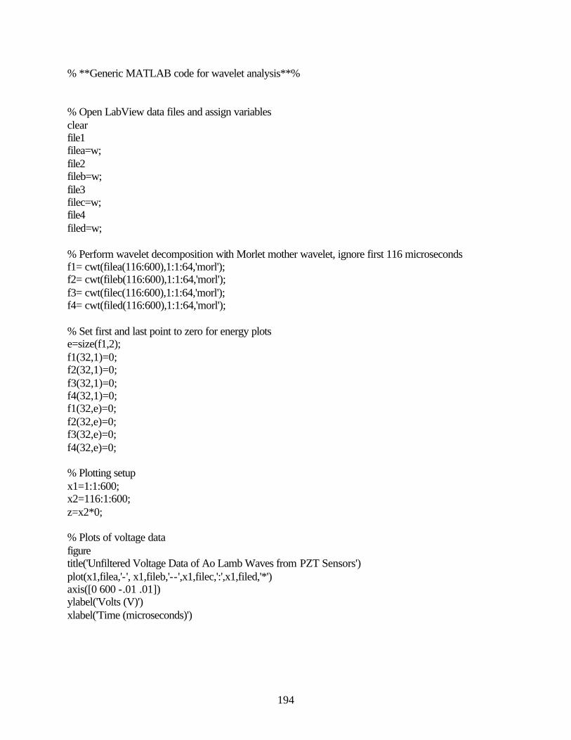
194
% **Generic MATLAB code for wavelet analysis**% % Open LabView data files and assign variables clear file1 filea=w; file2 fileb=w; file3 filec=w; file4 filed=w; % Perform wavelet decomposition with Morlet mother wavelet, ignore first 116 microseconds f1= cwt(filea(116:600),1:1:64,'morl'); f2= cwt(fileb(116:600),1:1:64,'morl'); f3= cwt(filec(116:600),1:1:64,'morl'); f4= cwt(filed(116:600),1:1:64,'morl'); % Set first and last point to zero for energy plots e=size(f1,2); f1(32,1)=0; f2(32,1)=0; f3(32,1)=0; f4(32,1)=0; f1(32,e)=0; f2(32,e)=0; f3(32,e)=0; f4(32,e)=0; % Plotting setup x1=1:1:600; x2=116:1:600; z=x2*0; % Plots of voltage data figure title('Unfiltered Voltage Data of Ao Lamb Waves from PZT Sensors') plot(x1,filea,'-', x1,fileb,'--',x1,filec,':',x1,filed,'*') axis([0 600 -.01 .01]) ylabel('Volts (V)') xlabel('Time (microseconds)')

195
% Plots of wavelet coefficient energy figure subplot(4,1,1) fill(x2,abs(f1(32,:)'),z) axis([116 600 0 .05]) ylabel('Dataset 1') title('Wavelet Coefficient Magnitudes for 15 kHz Signal Content') subplot(4,1,2) fill(x2,abs(f2(32,:)'),z) axis([116 600 0 .05]) ylabel(' Dataset 2') subplot(4,1,3) fill(x2,abs(f3(32,:)'),z) axis([116 600 0 .05]) ylabel(' Dataset 3') subplot(4,1,4) fill(x2,abs(f4(32,:)'),z) axis([116 600 0 .05]) ylabel(' Dataset 4') xlabel('Time (microseconds)')

196
APPENDIX E
LabView Codes for Experimental Procedures

197
Arb
itra
ry F
unct
ion
Gen
erat
or V
I
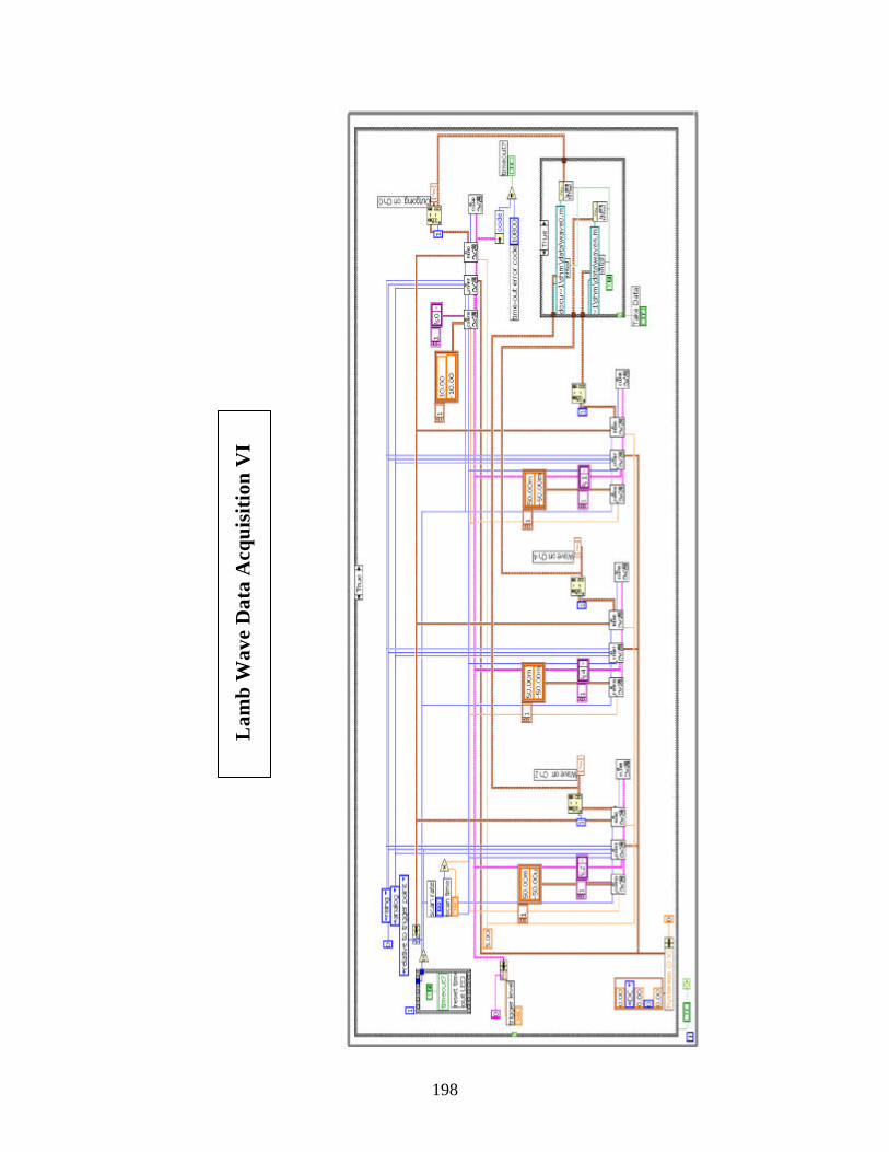
198
Lam
b W
ave
Dat
a A
cqui
siti
on V
I

199
Aco
usti
c E
mis
sion
Pen
cil B
reak
VI

200
Nar
row
Cou
pon
Ten
sile
Tes
t VI