Article

Piercing of Consciousness as a Threshold-CrossingOperation

Highlightsd Perceptual decisions can arise through an accumulation of

evidence to a threshold

d After a stimulus, participants set a clock to the moment they

had reached a decision

d An evidence accumulation model fit to these times allowed

predictions of accuracy

d The sense of having decided is mediated by a threshold on

accumulated evidence

Authors

Yul H.R. Kang,

Frederike H. Petzschner,

Daniel M. Wolpert, Michael N. Shadlen

Correspondenceshadlen@columbia.edu

In BriefDecision makers often feel there is a

moment of having reached a decision

during deliberation. Kang and Petzschner

et al. asked subjects to report this time by

setting a clock. The subjective decision

times predicted choice accuracy,

suggesting that awareness of completion

is mediated by a threshold crossing on

accumulated evidence.

Kang et al., 2017, Current Biology 27, 2285–2295August 7, 2017 ª 2017 The Authors. Published by Elsevier Ltd.http://dx.doi.org/10.1016/j.cub.2017.06.047

Current Biology

Article

Piercing of Consciousnessas a Threshold-Crossing OperationYul H.R. Kang,1,6 Frederike H. Petzschner,2,6 Daniel M. Wolpert,3 and Michael N. Shadlen1,4,5,7,*1Department of Neuroscience, Zuckerman Mind Brain Behavior Institute, Columbia University, New York, NY 10032, USA2Translational Neuromodeling Unit (TNU), Institute for Biomedical Engineering, University of Zurich and ETH Zurich, 8032 Zurich, Switzerland3Computational and Biological Learning Laboratory, Department of Engineering, Cambridge University, Cambridge CB2 1PZ, UK4Kavli Institute, Columbia University, New York, NY 10032, USA5Howard Hughes Medical Institute, Columbia University, New York, NY 10032, USA6These authors contributed equally7Lead Contact*Correspondence: shadlen@columbia.eduhttp://dx.doi.org/10.1016/j.cub.2017.06.047

SUMMARY

Many decisions arise through an accumulation of ev-idence to a terminating threshold. The process,termed bounded evidence accumulation (or driftdiffusion), provides a unified account of decisionspeed and accuracy, and it is supported by neuro-physiology in human and animal models. In many sit-uations, a decision maker may not communicate adecision immediately and yet feel that at some pointshe had made up her mind. We hypothesized thatthis occurs when an accumulation of evidence rea-ches a termination threshold, registered, subjec-tively, as an ‘‘aha’’ moment. We asked human partic-ipants to make perceptual decisions about the netdirection of dynamic random dot motion. The diffi-culty and viewing duration were controlled by theexperimenter. After indicating their choice, partici-pants adjusted the setting of a clock to the momentthey felt they had reached a decision. The subjectivedecision times (tSDs) were faster on trials with stron-ger (easier) motion, and they were well fit by abounded drift-diffusion model. The fits to the tSDsalone furnished parameters that fully predicted thechoices (accuracy) of four of the five participants.The quality of the prediction provides compelling ev-idence that these subjective reports correspond tothe terminating process of a decision rather than apost hoc inference or arbitrary report. Thus,conscious awareness of having reached a decisionappears to arise when the brain’s representation ofaccumulated evidence reaches a threshold orbound. We propose that such a mechanism mightplay a more widespread role in the ‘‘piercing of con-sciousness’’ by non-conscious thought processes.

INTRODUCTION

We are not consciously aware of all of the information deliveredfrom the senses to the brain, nor are we aware of the operations

that underlie the thoughts that do pierce consciousness. Indeed,the transition from non-conscious processing to consciousawareness is one of the great mysteries of psychology andneuroscience. In a series of classic studies, Libet and colleaguesused ‘‘mental chronometry’’ to identify the time that humanvolunteers felt they made a conscious decision to initiate amovement [1–3]. Libet suggested that this was the momentthat subjects ‘‘willed’’ their movement. He and others to followwere fascinated by the observation that neural events relatedto the movement could be detected hundreds of millisecondsbefore the subjects were aware [4], leading to philosophicalspeculation about volition and free will. However, it is unsurpris-ing that neural events would precede conscious awareness.Indeed, it has been suggested that the moment of awarenessmight reflect the completion of a decision process [5, 6]—inthis case, a commitment to a proposition to move.Studies of decision making in animals and humans indicate

that many decisions arise from an accumulation of evidence toa criterion. The process, termed bounded evidence accumula-tion or bounded drift diffusion, explains the speed and accuracyof many types of decisions, including recognition memory, foodpreference, and perceptual category [7–9]. The mechanism isespecially well suited to explain perceptual decisions that areinformed by a sequence of independent, noisy samples of evi-dence. For example, when humans and monkeys are asked todecide the net direction of motion (e.g., left versus right) of a dy-namic random dot display, their choices and reaction times (RTs)are explained by a model in which evidence is accumulated untilit reaches one of two bounds, thereby determining which deci-sion is made and marking the end of deliberation. The mecha-nism is supported by neural recordings in human, nonhumanprimates, and rodents, which demonstrate neural correlates ofevidence accumulation and termination thresholds [8, 10–15].Termination thresholds might also apply to decisions that are

not communicated immediately, as they are in reaction timestudies, but instead occur without any overt sign of completion.Even without time pressure, a decision maker might terminate adecision covertly before all of the evidence has been receivedand thus ignore potentially useful information. Without anaccompanying behavior, such termination has been deducedindirectly by analyzing decisions and showing that they are notaffected by the late arrival of evidence [16]. However, thisconclusion is not widely accepted [17]. We hypothesized that a

Current Biology 27, 2285–2295, August 7, 2017 ª 2017 The Authors. Published by Elsevier Ltd. 2285This is an open access article under the CC BY license (http://creativecommons.org/licenses/by/4.0/).

putative termination threshold might be registered, subjectively,as an ‘‘aha’’ moment, similar to the moment that Libet’s partici-pants reported about their will to move. We therefore set out totest whether mental chronometry marks decision termination.Up to now, it has been thought that objective validation of a sub-jective decision time is a logical impossibility, given the absenceof an objective manifestation with which to compare it [18]. How-ever, bounded evidence accumulation models furnish a test of astringent prediction: if subjective times correspond to decisiontermination, then they ought to predict decision accuracy.Here, we test this prediction and show that they do.

RESULTS

Experiment 1: Controlled Viewing Duration withSubjective Decision TimesFive participants performed a direction discrimination task inwhich they were asked to decide the net direction of dynamicrandom dots, viewed on a computer display (Figure 1A). The dif-ficulty of the decision was controlled by the probability, C, thateach dot will reappear Dt later, either at displacement, Dx, alongan axis of motion, or randomly replaced by a new dot (see STARMethods). We refer to C as the motion coherence (or motionstrength) and use its sign to indicate a direction. Both the direc-tion and strength of motion were randomized from trial to trial,and viewing duration was controlled by the experimenter. Be-sides the random dot motion, the display consisted of a centralfixation point, two ‘‘choice targets,’’ and a ‘‘clock’’. After the mo-tion display ended and an additional delay period, participants

indicated their decision about the direction of motion by usinga hand-held stylus to move a cursor to the left or right choicetarget. They were then asked to restore the clock ‘‘handle’’ tothe position it had attained at the moment they felt they haddecided the direction, what we term ‘‘subjective decisiontime’’. The participants received extensive training on the useof the clock (see STAR Methods and Methods S1 and S2), andwe ensured that they could use the clock accurately to reportthe time of an auditory cue presented at a random time duringmotion viewing (Figure S1).Subjective decision times (tSDs) varied as a function of motion

strength. The data in the top row of Figure 2 were obtained usinga motion stimulus duration of 800 ms. The tSDs were shortestwhen the motion was strong and longest when the motion wasweak. This pattern was statistically reliable for four of five sub-jects as well as at a group level (p < 10!6; GLM; see STARMethods). The pattern is qualitatively similar to mean responsetimes observed in free-response paradigms, in which viewersare allowed to indicate their decision with an action wheneverready (e.g., [20]). The solid blue curves in these panels are fitsof a parsimonious drift-diffusionmodel to themean tSDs (see Fig-ure 1B and STAR Methods), treating them as if they are reactiontimes. The idea is that a decision completes when the accumu-lation of noisy samples of evidence reaches an upper or lowerbound. The shape of the curve is determined by two parameters:(1) a term, k, that determines the evidence drawn at each timestep, dt, from a Gaussian distribution with mean kCdt and vari-ance dt and (2) the bound height, ±B. Translations along the ab-scissa and ordinate are captured by a coherence bias term (C0)

central fixation

delay, go cue& choice subjective

decision time

leftchoice target

rightchoice target

motion stimulus & clock rotation motion stimulus

disappears

FP

Time

visual stimulus

Dec

isio

n va

riabl

e(a

ccum

ulat

ed e

vide

nce)

left

right

ts

subjectivedecision time

Time (ms)0 800

0

+B

-B

on off

A

B

1200

cue torespond

400

200–800 ms

0.2 - 0.8 s

Figure 1. Subjective Report of DecisionTermination in a Perceptual Task(A) Controlled-duration task. On each trial, par-

ticipants fixated a central fixation point (FP).

A random dot motion stimulus then appeared at

the same time as a central clock started rotating.

Participants were asked to judge the direction of

motion (left versus right) and also the position of

the clock hand at the time they made their deci-

sion. After a computer-controlled time (0.2–0.8 s),

the motion stimulus was extinguished, and after a

delay (0.2–0.8 s), a tone sounded and participants

indicated the perceived motion direction by mov-

ing the cursor to one of two choice targets. They

then reported their subjective decision time by

moving a stylus to position the clock hand at the

remembered clock location at the time of their

decision about the motion direction (see STAR

Methods, Methods S1 and S2, and Figure S1).

(B) Information flow diagram showing visual

stimulus and hypothesized events leading to a

decision. The visual stimulus gives rise to a deci-

sion variable (black trace) that is the accumulation

of noisy evidence. The decision is complete when

a ‘‘right’’ or ‘‘left’’ bound is crossed (that is,

when ±B of evidence has accumulated). The

example illustrates a trial that gives rise to a

rightward choice with decision time around

500 ms, although the stimulus lasts 800 ms. Data

from neural recordings [16, 19] suggest that the

delay from motion onset to the beginning of the accumulation (ts) is around 200 ms. In general, the reported subjective decision time (tSD) might differ from the

actual moment of decision termination by additional delays attributed to perceptual and cognitive operations associated with storage and recall of the clock

position.

2286 Current Biology 27, 2285–2295, August 7, 2017

(see [21]) and a non-decision time (tND), respectively (parametersin Table 1). Based on the tND, the actual time of decision termina-tion occurred within the stimulus duration for subjects 1–4. Byeye, the fits capture the data reasonably well for all subjectsexcept subject 5. Thus, for four of the subjects, tSDs appear toconform to the same regularities as explicit reaction times. Toevaluate this assertion, the same diffusionmodel should accountfor the choices the subjects made about direction.The graphs in the lower row of Figure 2 show the influence of

motion strength and direction on the subjects’ choices. Deci-sions were perfectly accurate at the strongest motion strengths(leftmost and rightmost points) and near chance at the weakestmotion strengths (middle of the graph). Note that the dashedcurves are not fits to the data. They are predictions of thechoice proportions from the diffusion model using the parame-ters derived from the fits to the tSDs. If the tSDs reflect thetermination of a bounded diffusion process, then the choiceproportions are a logistic function of 2Bk(C ! C0), where C issigned motion strength. These predictions are remarkablygood for subjects 1–4 (p = 0.002, 0.005, 0.045, and 0.01,respectively; comparison with log likelihood of the observed

choices given shuffled tSDs; see STAR Methods). For the fifthsubject, not surprisingly, we could not use tSDs to predict thechoices (p = 0.71). Instead, we show the combined fit of thechoice and tSDs from this subject’s data (gray curves). The fitis driven primarily by the choice frequencies (lower panel).A group level analysis using the data from subjects 1–4 revealsthat choices were significantly better described by the predic-tions from the fit to each subject’s own tSDs than by a randomcombination of the parameters from the other subjects (none ofthe 531,441 combinations were better than the original; seeSTAR Methods). From these fits and predictions, we concludethat, for four of the subjects, the tSD reports correspond to thetermination of evidence accumulation and commitment to aperceptual decision.Our main conclusion rests on the capacity to predict the

choice functions. We wished to evaluate the assertion that thequality of these predictions suggests that tSDs were in fact indic-ative of actual terminations of a drift-diffusion process. Clearly,random reports of decision time would not yield sensible predic-tions, nor does the pattern of tSDs displayed by subject 5. How-ever, one might reasonably ask whether any systematic use of

Figure 2. Subjective Decision Times Reflect Termination of a Decision ProcessData are from five participants tested on a controlled-duration task for the trials in which the motion display lasted 800 ms. Subjective decision times (top) and

proportion of rightward choices (bottom) are plotted as a function of motion strength (negative and positive values indicate leftward and rightward direction,

respectively). Blue solid lines are drift-diffusion fits to the tSD data, and blue dashed lines are predictions using the parameters of the tSD fits (parameters in

Table 1). For subject 5, the gray lines are the joint fits to the tSD and choice. Points are means ± SEM.

Table 1. Parameters of the Drift-Diffusion Model Fit to the tSD Data in the Controlled-Duration Task

B k C0 tND

Subject 1 0.62 ± 0.01 40.4 ± 3.3 0.007 ± 0.004 0.131 ± 0.006

Subject 2 0.62 ± 0.13 5.7 ± 3.9 !0.053 ± 0.030 0.562 ± 0.166

Subject 3 0.74 ± 0.02 19.2 ± 2.6 !0.001 ± 0.006 0.790 ± 0.027

Subject 4 0.70 ± 0.02 24.3 ± 3.4 0.018 ± 0.007 0.227 ± 0.015

Subject 5 0.33 ± 0.10 24.6 ± 7.7 !0.050 ± 0.008 1.463 ± 0.050

Parameters are shown ±SE.

Current Biology 27, 2285–2295, August 7, 2017 2287

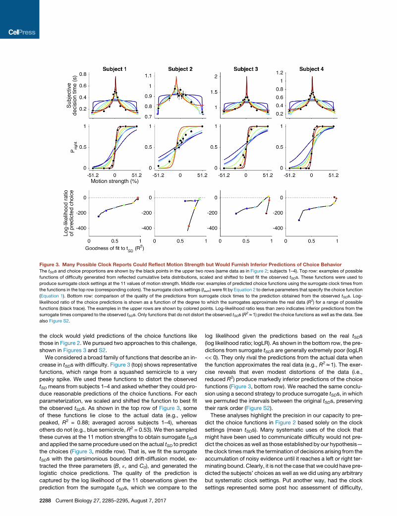
the clock would yield predictions of the choice functions likethose in Figure 2. We pursued two approaches to this challenge,shown in Figures 3 and S2.

We considered a broad family of functions that describe an in-crease in tSDs with difficulty. Figure 3 (top) shows representativefunctions, which range from a squashed semicircle to a verypeaky spike. We used these functions to distort the observedtSD means from subjects 1–4 and asked whether they could pro-duce reasonable predictions of the choice functions. For eachparameterization, we scaled and shifted the function to best fitthe observed tSDs. As shown in the top row of Figure 3, someof these functions lie close to the actual data (e.g., yellowpeaked, R2 = 0.88; averaged across subjects 1–4), whereasothers do not (e.g., blue semicircle, R2 = 0.53). We then sampledthese curves at the 11 motion strengths to obtain surrogate tSDsand applied the same procedure used on the actual tSD to predictthe choices (Figure 3, middle row). That is, we fit the surrogatetSDs with the parsimonious bounded drift-diffusion model, ex-tracted the three parameters (B, k, and C0), and generated thelogistic choice predictions. The quality of the prediction iscaptured by the log likelihood of the 11 observations given theprediction from the surrogate tSDs, which we compare to the

log likelihood given the predictions based on the real tSDs(log likelihood ratio; logLR). As shown in the bottom row, the pre-dictions from surrogate tSDs are generally extremely poor (logLR<< 0). They only rival the predictions from the actual data whenthe function approximates the real data (e.g., R2z1). The exer-cise reveals that even modest distortions of the data (i.e.,reduced R2) produce markedly inferior predictions of the choicefunctions (Figure 3, bottom row). We reached the same conclu-sion using a second strategy to produce surrogate tSDs, in whichwe permuted the intervals between the original tSDs, preservingtheir rank order (Figure S2).These analyses highlight the precision in our capacity to pre-

dict the choice functions in Figure 2 based solely on the clocksettings (mean tSDs). Many systematic uses of the clock thatmight have been used to communicate difficulty would not pre-dict the choices as well as those established by our hypothesis—the clock timesmark the termination of decisions arising from theaccumulation of noisy evidence until it reaches a left or right ter-minating bound. Clearly, it is not the case that we could have pre-dicted the subjects’ choices as well as we did using any arbitrarybut systematic clock settings. Put another way, had the clocksettings represented some post hoc assessment of difficulty,

Figure 3. Many Possible Clock Reports Could Reflect Motion Strength but Would Furnish Inferior Predictions of Choice BehaviorThe tSDs and choice proportions are shown by the black points in the upper two rows (same data as in Figure 2; subjects 1–4). Top row: examples of possible

functions of difficulty generated from reflected cumulative beta distributions, scaled and shifted to best fit the observed tSDs. These functions were used to

produce surrogate clock settings at the 11 values of motion strength. Middle row: examples of predicted choice functions using the surrogate clock times from

the functions in the top row (corresponding colors). The surrogate clock settings (tsurr) were fit by Equation 2 to derive parameters that specify the choice function

(Equation 1). Bottom row: comparison of the quality of the predictions from surrogate clock times to the prediction obtained from the observed tSDs. Log-

likelihood ratio of the choice predictions is shown as a function of the degree to which the surrogates approximate the real data (R2) for a range of possible

functions (black trace). The examples in the upper rows are shown by colored points. Log-likelihood ratio less than zero indicates inferior predictions from the

surrogate times compared to the observed tSDs. Only functions that do not distort the observed tSDs (R2z1) predict the choice functions as well as the data. See

also Figure S2.

2288 Current Biology 27, 2285–2295, August 7, 2017

they would have had to conform coincidentally to the functionalform of decision terminations that just so happened to predictthe choice proportions. These considerations bear on the mainalternatives to our hypothesis, considered below.Another feature of the data supports the interpretation that the

tSDs mark the termination of a decision process. In actual reac-tion time studies, in which subjects respond as soon as readywith an answer (unlike our experiment 1), it has been shownthat the full distribution of response latencies across trials is ex-plained by a more elaborate model of bounded evidence accu-mulation—in particular, one in which the flat bounds are replacedby time-dependent, collapsing bounds [22, 23]. We used such amodel to fit the tSD reports from the controlled-duration task (Fig-ure S3). As shown in Figure 4, the conformance to data is impres-sive for subjects 1–4 but less so for subject 5. To quantify thegoodness of fit, we calculated the Jensen-Shannon divergence(JSD) between the fitted and observed distributions for each ofthe five subjects (Figure S4). Random shuffling of the fitted andobserved distributions across motion strengths supports rejec-tion of the null hypothesis that the quality of the fit would ariseby chance, knowing only choice proportions and the mean tSDvalues (p < 0.02, subjects 1–4; p > 0.9, subject 5). We used abootstrap procedure to obtain confidence intervals on the JSD(error bars; Figure S4), which, not surprisingly, identifies subject 5as an outlier. The ability to explain the distribution of tSDs makesit all the more unlikely that the clock settings from subjects 1–4represent anything other than termination of an accumulationof noisy evidence.Finally, we analyzed themotion information in the RDM itself to

test whether the subjective decision times demarcate comple-tion of the decisions. According to our hypothesis, motion infor-mation in the display should support the choice only up to thetime that the accumulated noisy evidence reaches a bound.On each trial, we estimated this time (tq) from the clock reportminus the non-decision time obtained from the fits in Figure 2using the three weakest motion strengths and asked whetherthe information before or after tq was the more informative aboutthe subsequent choice. To place these motion energy compari-sons on equal footing, we always used the first and last half(400 ms each) of the display (Figure 5A, inset). Importantly, werestricted the analysis to trials in which tq was close to thismidpoint. To increase the power of the analysis, we examineda range of tolerances on tq by requiring it to be within ±D ms ofthe midpoint, thereby varying the number of trials that met thecriterion. Figure 5A compares the leverage of the integrated mo-tion energy before and after the midpoint on choice, controllingfor motion strength (logistic regression; see STAR Methods).The leftmost red and blue points contain data from the 82 trialsin which tq was within 400 ± 13.3 ms from motion onset (i.e.,video frames 30 and 31). By widening the acceptance windowto 400 ± 26.6 ms (170 trials), we achieve greater power and inferthe greatest leverage of the motion information before themidpoint. The graph shows that widening the tolerance (so thateventually all trials are included) leads to a gradual dissipationof the leverage of the motion energy before the midpoint andan increase in the leverage of information after 400 ms. At largertolerance, the before/after designation no longer matters.Because we always used the first and second halves of the

display to perform these calculations, a possible concern is

that the division at 400 ms merely reflects the fact that earlystimulus information is more influential than late and says littleabout whether the tq are informative. To evaluate this, we per-formed a bootstrap analysis (n = 5,000), in which we comparedthe leverage of the pre- and post-400-ms motion energy on tri-als with a tq within ±133 ms window of the midpoint with thosewith tq outside this window (Figure 5B). We chose this windowto balance power against dissipation of the effect (see STARMethods). We evaluated the null hypothesis that the differencein leverage for the pre- and post-400-ms motion energy wasthe same for these two sets of trials. This showed that thepre-400-ms motion energy had significantly more leveragethan the post-400-ms motion energy on choice only when tqwas within the ±133 ms window (p < 0.007; one-tailed). Thisheld for many windows from 26 to 160 ms (six p < 0.05 andfive p < 0.1).

Experiment 2: Free Response with Subjective DecisionTimesAccording to our hypothesis, tSDs mark the termination of thesame type of process that gives rise to reaction times, when sub-jects control their viewing time. We therefore collected data on afree-response version of the task from the same subjects afterthey completed the first experiment. All aspects of the task,including the clock, were the same as the version above, exceptthat, instead of waiting for the random dots to disappear after apreset duration, the participant reported each decision as soonas she was ready by moving the stylus to one of the choicetargets and subsequently set the clock to report a subjectivedecision time. The tSDs in this experiment are not particularly illu-minating, because they might be coupled to reaction times evenif they did not indicate decision termination. However, they doserve as a sanity check, and in this regard, it is reassuring thatthe tSDs were indeed correlated with RTs (Pearson’s r = 0.80–0.96; p < 10!10), consistent with previous studies [24–26]. Forsubjects 1–4, most tSDs preceded the RTs (range 52%–98%).For subject 5, only 15% of the tSDs preceded the RTs, consis-tent with the observation that this participant deployed the clocksettings differently than the others. Presumably, the decision toreport and the decision to move are not the same process, justas the decision to report with a saccade or a reach movementis subserved by different circuits [27, 28]. Therefore, in principle,the decision to report could occur after the decision to move thestylus, using information from the randomdot display that did notarrive in time to affect the hand movement [29–31]. Indeed, inalmost all of the trials in which the RT preceded tSDs, the differ-ence was less than 400ms (99.5% of all trials and 97%of trials inwhich the RT preceded tSDs, across subjects 1–4).The choice and reaction time data from all five subjects were

well described by bounded drift diffusion (Figure 6). The blackcurves are fits of the parsimonious model, used above, to thechoice-reaction time data from the free-response task. Theyare joint fits to both sets of observations—choice and RT—ratherthan predictions (parameters in Table S1). The fitted boundheight was higher in the free-response task, but this is not sur-prising because subjects could avail themselves of up to 2.7 sof evidence in this task, compared to a maximum of 800 ms inthe controlled-duration task. In contrast, we reasoned that theparameter, k, should be similar in the two experiments, because

Current Biology 27, 2285–2295, August 7, 2017 2289

it represents the conversion of motion strength to the signal-to-noise ratio of momentary evidence, which tends to be stablewhen humans and monkeys alter their speed-accuracy tradeoffor their bias [10, 21]. As shown in Figure S5, the scaling param-eters, k, estimated from the two tasks were similar for the sub-jects (Pearson’s r = 0.97, p = 0.007 for subjects 1–5; r = 0.97,

p = 0.032 with subject 5 removed). Indeed, the red curves in Fig-ure 6 for subjects 1–4 are fits that constrain k to the value derivedfrom the tSDs in the controlled-duration task (Table S2; forsubject 5, we used k from the joint fit to choice-tSD data). Thesimilarity to the black curves implies that deducing the signal-to-noise parameter solely from subjective reports of the time of

Figure 4. Distribution of tSDsEach row represents a coherence level, each column a subject. Ordinate is proportion of responses with the tSDs from the controlled-duration experiment, signed

by the direction of response (positive, right; negative, left). The scale of each row is normalized to fit the row’s height for visualization. Black lines are the data, and

blue lines are the drift diffusion fit with collapsing bounds (parameters in Table S3). The data are smoothed in time with a Gaussian kernel (s = 0.05 s) for

visualization. Goodness of fit, quantified by the Jensen-Shannon divergence, is displayed in Figure S4. The more elaborate model also accounts for the reaction

time distributions (and slow errors) in the free-response task (data not shown). See also Figure S3.

2290 Current Biology 27, 2285–2295, August 7, 2017

decision completion in the controlled-duration task predicted akey parameter of the mechanism that would give rise to deci-sions in a later experiment.These observations (Figures 6 and S5) lend further support to

our hypothesis that a common mechanism supports decisiontimes reported explicitly or via mental chronometry. They alsounderscore the counterexample of subject 5, because the con-sistency of k demonstrates that he used a similar mechanismof evidence accumulation to make decisions on the controlled-duration and free-response tasks, yet the tSDs obtained in thecontrolled-duration task were uninformative.

Alternative HypothesesWe considered several alternative explanations of the subjectivereports, which would imply that they are not signatures of deci-sion termination. One possibility is that the tSDs do not representa termination at all because the subjects used all of the informa-tion in the motion display to form their decisions. This alternativecannot explain the capacity to use the tSDs to predict the choicefrequencies (Figure 2), and it is directly refuted by the analyses ofmotion energy in Figure 5, which shows that subjects ignore late-arriving information when the inferred termination times are nearthe midpoint of the trial.Another class of alternatives would allow for early termination

of evidence accumulation but posit that such events are not re-flected in the tSDs. For example, the reports might be assigned,inferentially or postdictively, to a moment between the start andend of the dot motion [32–34]. The subject could believe in theexperience of completing the decision, but it would have no cor-respondence to the actual time of commitment [35]. This is anintriguing idea, but it fails to account for the dependency oftSDs on motion strength. Any reasonable alternative must ac-count for this regularity. For example, the subjects might haveused the clock as a rating scale for difficulty, setting the clocknearer the starting position when the stimulus appeared morecoherent (or felt easier). There are three reasons to reject thisalternative: (1) monotonic transformations of difficulty are gener-ally incapable of achieving choice predictions unless they

happen to be nearly identical to tSDs (Figures 3 and S2); (2) theidea provides no explanation for the distribution of tSDs acrosstrials (Figure 4), and (3) it fails to explain the difference in leverageof the early and late motion information on choice—specifically,the sensitivity of this analysis to the use of the corresponding tri-al’s tSD (Figure 5). These considerations rule out most ‘‘clock asrating scale’’ alternatives, but there is one that remains.It has been shown that elapsed decision time bears on confi-

dence that a decision is correct [36], and for some observers,elapsed time is more important than motion strength. It mighttherefore be argued that, despite the instruction to indicate thetime of a decision, subjects used the clock as a rating scale,placing the hand closer to its initial position if they were moreconfident. However, this possibility is incompatible with obser-vations on the subset of trials in which motion was displayedfor only 200 ms. Not surprisingly, subjects were less sensitiveto the motion on these trials compared to trials with motion dis-played for 800ms (p < 0.002 for all except subject 2, whose trendwas of the same sign: p = 0.32; see Figure S6), yet the tSDs wereshorter (Dduration range: !401 ms to !64 ms; p < 10!6). If theclock settings were a report of confidence, they should haveexhibited the opposite trend. We conclude that four of the fivesubjects reported tSDs that were linked to the time of decisiontermination, as they were instructed.

DISCUSSION

Our findings exploit a well-studied task that has been used toexpose the neural mechanisms of a perceptual decision.Although the decision is about a perceptual quality or category,the task is less a model of perception, which is typically fast[37, 38], and more like the kind of deliberative decisions wemake over more prolonged intervals based on a sequence ofsamples of evidence [39, 40]. Its main advantages are the quan-titative agreement with the mathematical depiction of boundedevidence accumulation and the correspondence with neural re-cordings, mainly from rhesus monkeys (e.g., [8, 41]). Thus, it fur-nishes an empirical test of the hypothesis that the feeling of

A B Figure 5. Effect of Trial-to-Trial Variation inthe Noisy Motion Information on ChoiceThe analysis compares the leverage of information

before and after a putative threshold crossing that

terminates integration. Leverage is based on

logistic regression of motion energy (right minus

left; see STAR Methods), controlling for motion

strength.

(A) Leverage of early- and late-motion energy (blue

and red, respectively). The estimates are shown as

a function of the inclusion window. Pairs of points

include only trials with estimated termination times

(tq) near 400 ms. (Inset shows how the putative

termination time tq is acquired on each trial. It is the

tSD from the clock setting minus the non-decision

time estimated from the fits in Figure 2, top

row). Filled symbols designate non-zero leverage

(p < 0.05). Larger tolerances permit inclusion of more trials but blur the distinction between pre- and post-tq. Error bars indicate SE.

(B) Difference in the leverage of motion energy before and after 400 ms requires tq to be near 400 ms. The bars on the right side show the leverage values using

tolerance of ±133 ms (same value and SE as the points in A marked by arrows). Bars on the left show the average leverages obtained by sampling the com-

plementary trials with tq outside this tolerancewindow (5,000 bootstraps of sets of 873 trials; error bars are average of the SE from the bootstraps). The distribution

of differences (b1–b2) rarely exceeds the observed difference (p < 0.007). Combined data from subjects 1–4 using motions strengths 0%, ±3.2%, and ±6.4%

coherence.

Current Biology 27, 2285–2295, August 7, 2017 2291

‘‘having decided’’ corresponds to a threshold crossing thatmarks themoment that the accumulated evidence reaches a ter-minating bound.

In a free-response experiment, there is an overt manifestationof decision termination, namely the reaction time, whereas, inour controlled-duration experiment, there is only the memoryof the time of the feeling of having decided—that is, the clocksettings (tSDs). Without another indication of when the decisionterminated, it might seem impossible to associate tSDs withtermination of the decision [18]. However, we reasoned that wecould overcome this limitation by using the tSDs to account forthe one other experimental observation: the choices. We fit thetSDs to a bounded evidence accumulation model to derive threeparameters (k, B, and C0) that would fully specify the choice fre-quencies as a function of motion strength. The success of thesepredictions was remarkable in four of the five subjects. Thus, weconclude that the time that these subjects reported that they haddecided does indeed mark the time of decision termination. It isnot the actual time but offset by a constant, analogous to themotor preparatory component of the reaction times in a free-response experiment (see below).

Had the subjects indicated their choices at the time they madethem, we would suspect that their clock settings merely indi-cated the time of the action—that is, a post hoc report of anotherprocess, such as movement of the stylus. In that case, we couldnot argue that they mark a subjective awareness of decisiontermination. This is a reasonable interpretation of the tSDs inthe free-response task, but not in the controlled-duration task,in which subjects only indicated their response after a variabledelay period. There was no event in the experiment or the sub-ject’s behavior that could be assigned a time on the clock exceptfor the one that the subjects were asked to note—the feeling thatthey had made up their mind.

One might argue that the subjects were performing a mockfree-response task in their mind and reporting tSDs at the timeof their planned action. This is unlikely because four of the sub-

jects had never experienced a reaction time experiment and wedid not introduce the free-response task until after data collectionwas completed on the controlled viewing duration task. There is,of course, a sense in which this proposal is consistent with ourinterpretation. We have argued forcefully that the subjective deci-sion timesmark a mental event that is mediated by a threshold onthe evidence accumulation—that is, the same type of processthat underlies decision termination in a free-response (reactiontime) experiment. Finally, we cannot rule out the possibility thatsubjects changed their mind (e.g., see [29, 42]), but that is likelyto have involved only a small fraction of trials.There are several important implications of our result. First, it

confirms that the brain exercises a stopping criterion on a streamof evidence, even when the environment (or experimenter) con-trols the duration of the stream of evidence [16, 17]. Put anotherway, even when there is no overt measure of reaction time, de-cision makers terminate their decisions in a manner similar tothe way they would if they were responding when ready. It sug-gests that accuracy in simple two-alternative, forced-choice ex-periments is not determined solely by considerations of signal tonoise, as commonly assumed, but the speed-accuracy policyadopted by the subject. Without a measure of RT, the speed ofa decision is not known, but it is conceivable that variation in ac-curacy among individuals and during learning reflects differ-ences in the speed-accuracy trade-off, even when there is nooutward manifestation of decision time. The present studyshows that this time may be consciously registered as an‘‘aha’’ moment, available to the decision maker if asked (orknew she would be asked).A second implication concerns mental chronometry itself—

that is, the validity of the clock report. It has been argued thatsuch reports may be too unreliable or too biased to mark actualmental events [26, 43, 44]. Further, without an objective measureof the mental event, it seemed impossible to validate that thething being timed had actually occurred at that time or at somelawful latency. The present findings support the validity of the

Figure 6. Reaction Times and Choices in the Free-Response TaskReaction times (top) and proportion of rightward choices (bottom) are plotted as a function of motion strength for the five subjects (mean ± SEM). Solid lines are

drift-diffusion fits to RT and choice data (black; parameters in Table S1). Red curves show fits with k fixed to the parameters from the tSD fits for each subject in the

controlled-duration task (parameters in Table S2). See also Figure S5.

2292 Current Biology 27, 2285–2295, August 7, 2017

clock reports. No doubt they are imprecise, but the conformanceto actual RT distributions suggests that some of the imprecisionis a reflection of the variability of mental events themselves. Weprovide an example in which they are tied to a mental event thathas no external manifestation and thus seems to be untestable,just as in the Libet experiments. However, we showed that theevent had predictive power and that it corresponds to the typeof termination events that lead to reaction times in other experi-ments, including the free-response experiment with our sub-jects. We cannot argue that mental chronometry is valid in othersettings, such as the Libet experiments. However, to the extentthat an urge tomove (as in Libet) is effectively a decision tomove,we are inclined to think so.Like actual RTs, the time of the report—be it a movement or a

mental note of the position of the clock—differs from the time ofthe decision. This discrepancy, termed the non-decision time(tND) in RT experiments, is typically 300–400 ms for motiondiscrimination, depending on the response modality. Electro-physiology in the monkey suggests that "200 ms of this tND isin the time it takes information in the video display to impactthe representation of the accumulated evidence [19]. The restof the tND is accounted for by a latency between the terminationof the accumulation and initiation of the motor response. Formental chronometry, the tND might comprise systematic biasesin the perception of the clock position or the recall of the positionor both, as argued by skeptics of Libet’s use and interpretations(e.g., [43, 45]). This does not negate the validity of tND, however,as it allows us to infer the decision time (tq) from the subjectivereport to predict not only the choices but an approximate pointin time that divides the stimulus into information used andignored on the trial (Figure 5).The intriguing insight furnished by the present study is that the

moment of subjective awareness of having decided reflects thetermination of a decision process. Here, there is substantial ev-idence that decision termination is mediated by application of athreshold to the neural representation of accumulating evidence[8, 46, 47], and this also holds in experiments that do not allowfor free responses, as in our controlled-duration experiment[13, 16, 48]. This operation may be more widespread, asmany mental processes achieve a state of completion, whichis effectively a decision point. Of course, not all involve a choiceamong discrete propositions, like the motion discriminationtask; nor are all as simple as a decision to commence a move-ment, as in Libet’s studies. Some might involve a transition orbranching from one step of reasoning to another in more com-plex problems involving strategy (e.g., foraging and medicaldiagnosis). The common feature is a satisfaction of some termi-nation criterion before proceeding. Such termination events donot result invariably in conscious awareness, but the subjectivedecision times assessed here (and by Libet) do necessitateconscious awareness, by definition. Indeed, the main distinctionbetween non-conscious and conscious decisions might besimply the possibility of reporting in some way, even if only pro-visionally [5]. Thus, we suggest that the neurophysiological pro-cess responsible for completing the decision to report is alsoresponsible for piercing conscious awareness. This assertionmay not satisfy philosophers who postulate a distinction be-tween what is reportable and what is in conscious awareness(e.g., access and phenomenal consciousness [49]). These phi-

losophers might think it is possible for consciousness aware-ness to lag behind the decision to report. There may be someroom in the non-decision time to countenance this argument,but it is narrow.The capacity to report is the criterion we use informally to

query whether an agent is consciously aware of something,but it has a deeper significance. We speculate that the decisionto report—even if only provisionally—is the common elementconnecting those mental processes that pierce consciousawareness. Consider that non-conscious knowledge of objects(e.g., position, shape, and desirability) corresponds to affordan-ces [50], a term that refers to ways of interacting with the object(e.g., position for looking, shape for grasping, and desirability foreating, mating, or fleeing). These provisional affordances conferproperties that are as much about our possible actions as theyare about the object. The possibility of reporting a feature of anobject to another agent—or to oneself in the future (e.g., usingepisodicmemory)—changes the balance away frommy possibleactions and toward the object, which inhabits not just the per-sonal space of my own actions but also the mental space ofanother’s mind [51]. For example, the location of the object tran-scends my personal frame of reference, and the object itselfseems to possess qualities that are independent of my ac-tions—an essence, as it were [52]. These philosophical specula-tions concern the content of conscious experience (e.g., what itis that we might report), whereas the tSDs in our experimentmerely mark the time that the subject decided to possibly renderit. Of course, many decisions arise without triggering a decisionto report, and these remain unconscious to us.Importantly, we do not claim that our subjects were not

conscious of the deliberation process itself. They might havebeen consciously aware of some or all of the random dot mo-tion leading to the decision. There are two ways to accountfor this within our framework. First, the visual system mightanalyze other features of the random dot display and reach pro-visional decisions to report (e.g., a cluster of dots resembling ageometric shape). Second, during deliberation, one might reacha decision by applying a lower threshold but then change one’smind [29, 30] or reaffirm by applying a more conservativethreshold. Each of these mini-decisions might pierce con-sciousness. Second, when a process pierces consciousness,it carries with it content and associations that are there to be re-ported as well. Some of this content could be in visual workingmemory (e.g., appearance of some pattern in the dots) or work-ing memory of the experience of deliberating [53], what issometimes referred to as metacognition [54]. These explana-tions are not mutually exclusive. In the first, there are manypiercings. In the second, there could be only one, with contentfrom the past. Our experimental findings do not address thesecond idea, as we only asked participants to report left andright and the moment that they ‘‘felt they had decided in theirmind’’ (see STAR Methods). Rather, they suggest that thepiercing of conscious awareness might be mediated by a pro-cess resembling the termination of simpler decisions with overtmanifestations of completion (e.g., reaction time). This raisesthe intriguing possibility that consciousness itself may be closerto a neuroscientific explanation than is commonly thought, asknowledge of the neurobiology of decision making is rapidlyadvancing.

Current Biology 27, 2285–2295, August 7, 2017 2293

STAR+METHODS

Detailed methods are provided in the online version of this paperand include the following:

d KEY RESOURCES TABLEd CONTACT FOR REAGENT AND RESOURCE SHARINGd EXPERIMENTAL MODEL AND SUBJECT DETAILSd METHOD DETAILS

B ApparatusB TasksB TrainingB Computational ModelingB Evidence Accumulation Model with Flat BoundsB Model with Collapsing Bounds

d QUANTIFICATION AND STATISTICAL ANALYSISB Data Processing and AnalysisB Sensitivity analysis of choice predictionsB Analysis of motion energy

d DATA AND SOFTWARE AVAILABILITY

SUPPLEMENTAL INFORMATION

Supplemental Information includes six figures, three tables, and two methods

files and can be found with this article online at http://dx.doi.org/10.1016/j.

cub.2017.06.047.

AUTHOR CONTRIBUTIONS

Conceptualization, M.N.S., F.H.P., and Y.H.R.K.; Methodology, Y.H.R.K.,

F.H.P., D.M.W., and M.N.S.; Software, Y.H.R.K., F.H.P., D.M.W., and

M.N.S.; Formal Analysis, Y.H.R.K. F.H.P., D.M.W., and M.N.S.; Writing – Orig-

inal Draft, Y.H.R.K. and F.H.P.; Writing – Review & Editing, D.M.W. andM.N.S.;

Funding Acquisition, D.M.W. and M.N.S.; Investigation, Y.H.R.K. and F.H.P.;

Visualization, Y.H.R.K., F.H.P., D.M.W., and M.N.S.; Resources and Supervi-

sion, M.N.S.

ACKNOWLEDGMENTS

We thank Esther Kim, Ted Metcalfe, and Jian Wang for their technical assis-

tance and Danique Jeurissen, Chris Fetsch, John Morrison, and Ariel Zylber-

berg for constructive comments on the manuscript. The research was sup-

ported by the Howard Hughes Medical Institute and National Eye Institute

grant R01 EY11378 to M.N.S., the Human Frontier Science Program to

D.M.W. and M.N.S., the Wellcome Trust and Royal Society (Noreen Murray

Professorship in Neurobiology) to D.M.W., National Eye Institute grant T32

EY013933 to Y.H.R.K., and the Ren!e and Susanne Braginsky Foundation

and University of Zurich to F.H.P.

Received: March 24, 2017

Revised: May 23, 2017

Accepted: June 19, 2017

Published: July 27, 2017

REFERENCES

1. Libet, B. (2002). The timing of mental events: Libet’s experimental findings

and their implications. Conscious. Cogn. 11, 291–299, discussion

304–333.

2. Libet, B. (2003). Timing of conscious experience: reply to the 2002 com-

mentaries on Libet’s findings. Conscious. Cogn. 12, 321–331.

3. Libet, B., Gleason, C.A., Wright, E.W., and Pearl, D.K. (1983). Time of

conscious intention to act in relation to onset of cerebral activity (readi-

ness-potential). The unconscious initiation of a freely voluntary act. Brain

106, 623–642.

4. Soon, S.C., Brass, M., Heinze, H.J., and Haynes, J.D. (2008). Unconscious

determinants of free will in the human brain. Nat. Neurosci. 11, 543–545.

5. Shadlen, M.N., and Kiani, R. (2011). Consciousness as a decision to

engage. In Characterizing Consciousness: From Cognition to the Clinic?

Research and Perspectives in Neurosciences, S. Dehaene, and Y.

Christen, eds. (Springer), pp. 27–46.

6. Dehaene, S., Charles, L., King, J.-R., and Marti, S. (2014). Toward a

computational theory of conscious processing. Curr. Opin. Neurobiol.

25, 76–84.

7. Ratcliff, R. (1978). A theory of memory retrieval. Psychol. Rev. 85, 59–108.

8. Gold, J.I., and Shadlen, M.N. (2007). The neural basis of decision making.

Annu. Rev. Neurosci. 30, 535–574.

9. Rangel, A., Camerer, C., and Montague, P.R. (2008). A framework for

studying the neurobiology of value-based decision making. Nat. Rev.

Neurosci. 9, 545–556.

10. Hanks, T., Kiani, R., and Shadlen, M.N. (2014). A neural mechanism of

speed-accuracy tradeoff in macaque area LIP. eLife 3, e02260.

11. Shadlen, M.N., and Newsome, W.T. (2001). Neural basis of a perceptual

decision in the parietal cortex (area LIP) of the rhesus monkey.

J. Neurophysiol. 86, 1916–1936.

12. Huk, A.C., and Shadlen, M.N. (2005). Neural activity in macaque parietal

cortex reflects temporal integration of visual motion signals during percep-

tual decision making. J. Neurosci. 25, 10420–10436.

13. Ploran, E.J., Nelson, S.M., Velanova, K., Donaldson, D.I., Petersen, S.E.,

and Wheeler, M.E. (2007). Evidence accumulation and the moment of

recognition: dissociating perceptual recognition processes using fMRI.

J. Neurosci. 27, 11912–11924.

14. O’Connell, R.G., Dockree, P.M., and Kelly, S.P. (2012). A supramodal

accumulation-to-bound signal that determines perceptual decisions in hu-

mans. Nat. Neurosci. 15, 1729–1735.

15. Hanks, T.D., Kopec, C.D., Brunton, B.W., Duan, C.A., Erlich, J.C., and

Brody, C.D. (2015). Distinct relationships of parietal and prefrontal cortices

to evidence accumulation. Nature 520, 220–223.

16. Kiani, R., Hanks, T.D., and Shadlen, M.N. (2008). Bounded integration in

parietal cortex underlies decisions even when viewing duration is dictated

by the environment. J. Neurosci. 28, 3017–3029.

17. Tsetsos, K., Gao, J., McClelland, J.L., and Usher, M. (2012). Using time-

varying evidence to test models of decision dynamics: bounded diffu-

sion vs. the leaky competing accumulator model. Front. Neurosci. 6, 79.

18. Haggard, P. (2005). Conscious intention and motor cognition. Trends

Cogn. Sci. 9, 290–295.

19. Roitman, J.D., and Shadlen, M.N. (2002). Response of neurons in the

lateral intraparietal area during a combined visual discrimination reaction

time task. J. Neurosci. 22, 9475–9489.

20. Palmer, J., Huk, A.C., and Shadlen, M.N. (2005). The effect of stimulus

strength on the speed and accuracy of a perceptual decision. J. Vis. 5,

376–404.

21. Hanks, T.D., Mazurek, M.E., Kiani, R., Hopp, E., and Shadlen, M.N. (2011).

Elapsed decision time affects the weighting of prior probability in a

perceptual decision task. J. Neurosci. 31, 6339–6352.

22. Drugowitsch, J., Moreno-Bote, R., Churchland, A.K., Shadlen, M.N., and

Pouget, A. (2012). The cost of accumulating evidence in perceptual deci-

sion making. J. Neurosci. 32, 3612–3628.

23. Ditterich, J. (2006). Evidence for time-variant decision making. Eur. J.

Neurosci. 24, 3628–3641.

24. Corallo, G., Sackur, J., Dehaene, S., and Sigman, M. (2008). Limits on

introspection: distorted subjective time during the dual-task bottleneck.

Psychol. Sci. 19, 1110–1117.

25. Marti, S., Sackur, J., Sigman, M., and Dehaene, S. (2010). Mapping intro-

spection’s blind spot: reconstruction of dual-task phenomenology using

quantified introspection. Cognition 115, 303–313.

2294 Current Biology 27, 2285–2295, August 7, 2017

26. Miller, J., Vieweg, P., Kruize, N., and McLea, B. (2010). Subjective reports

of stimulus, response, and decision times in speeded tasks: how accurate

are decision time reports? Conscious. Cogn. 19, 1013–1036.

27. de Lafuente, V., Jazayeri, M., and Shadlen, M.N. (2015). Representation of

accumulating evidence for a decision in two parietal areas. J. Neurosci. 35,

4306–4318.

28. Scherberger, H., and Andersen, R.A. (2007). Target selection signals for

arm reaching in the posterior parietal cortex. J. Neurosci. 27, 2001–2012.

29. Resulaj, A., Kiani, R., Wolpert, D.M., and Shadlen, M.N. (2009). Changes of

mind in decision-making. Nature 461, 263–266.

30. van den Berg, R., Anandalingam, K., Zylberberg, A., Kiani, R., Shadlen,

M.N., andWolpert, D.M. (2016). A commonmechanism underlies changes

of mind about decisions and confidence. eLife 5, e12192.

31. Burk, D., Ingram, J.N., Franklin, D.W., Shadlen, M.N., and Wolpert, D.M.

(2014). Motor effort alters changes of mind in sensorimotor decision mak-

ing. PLoS ONE 9, e92681.

32. Kolers, P.A., and von Grunau, M. (1976). Shape and color in apparent mo-

tion. Vision Res. 16, 329–335.

33. Eagleman, D.M., and Sejnowski, T.J. (2000). Motion integration and post-

diction in visual awareness. Science 287, 2036–2038.

34. Geldard, F.A., and Sherrick, C.E. (1972). The cutaneous ‘‘rabbit’’:

a perceptual illusion. Science 178, 178–179.

35. Dennett, D.C. (1993). Consciousness Explained (Penguin).

36. Kiani, R., Corthell, L., and Shadlen, M.N. (2014). Choice certainty is

informed by both evidence and decision time. Neuron 84, 1329–1342.

37. Watson, A.B. (1986). Temporal sensitivity. In Handbook of Perception and

Human Performance, K.R. Boff, L. Kaufman, and J.P. Thomas, eds.

(Wiley), pp. 6-1–6-43.

38. Thorpe, S., Fize, D., and Marlot, C. (1996). Speed of processing in the hu-

man visual system. Nature 381, 520–522.

39. Kira, S., Yang, T., and Shadlen, M.N. (2015). A neural implementation of

Wald’s sequential probability ratio test. Neuron 85, 861–873.

40. Shadlen, M.N., and Shohamy, D. (2016). Decision making and sequential

sampling from memory. Neuron 90, 927–939.

41. Shadlen, M.N., and Kiani, R. (2013). Decision making as a window on

cognition. Neuron 80, 791–806.

42. Kiani, R., Cueva, C.J., Reppas, J.B., and Newsome, W.T. (2014).

Dynamics of neural population responses in prefrontal cortex indicate

changes of mind on single trials. Curr. Biol. 24, 1542–1547.

43. Lau, H.C., Rogers, R.D., and Passingham, R.E. (2006). On measuring the

perceived onsets of spontaneous actions. J. Neurosci. 26, 7265–7271.

44. Banks, W.P., and Isham, E.A. (2009). We infer rather than perceive the

moment we decided to act. Psychol. Sci. 20, 17–21.

45. Haggard, P. (2008). Human volition: towards a neuroscience of will. Nat.

Rev. Neurosci. 9, 934–946.

46. Churchland, A.K., Kiani, R., Chaudhuri, R., Wang, X.J., Pouget, A., and

Shadlen, M.N. (2011). Variance as a signature of neural computations dur-

ing decision making. Neuron 69, 818–831.

47. Smith, P.L., and Ratcliff, R. (2004). Psychology and neurobiology of simple

decisions. Trends Neurosci. 27, 161–168.

48. Mazurek, M.E., Roitman, J.D., Ditterich, J., and Shadlen, M.N. (2003).

A role for neural integrators in perceptual decision making. Cereb.

Cortex 13, 1257–1269.

49. Block, N. (1995). On a confusion about a function of consciousness.

Behav. Brain Sci. 18, 227–247.

50. Gibson, J.J. (1977). The theory of affordances. In Perceiving, Acting, and

Knowing: Toward an Ecological Psychology, R. Shaw, and J. Bransford,

eds. (Lawrence Erlbaum Associates), pp. 67–82.

51. Frith, C.D., and Frith, U. (1999). Interacting minds–a biological basis.

Science 286, 1692–1695.

52. Merleau-Ponty, M. (1962). Phenomenology of Perception (Routledge).

53. Amano, K., Qi, L., Terada, Y., andNishida, S. (2016). Neural correlates of the

time marker for the perception of event timing. eNeuro 3, ENEURO.0144-

16.2016.

54. Fleming, S.M., and Dolan, R.J. (2012). The neural basis of metacognitive

ability. Philos. Trans. R. Soc. Lond. B Biol. Sci. 367, 1338–1349.

55. Newsome, W.T., Britten, K.H., Salzman, C.D., and Movshon, J.A. (1990).

Neuronal mechanisms of motion perception. Cold Spring Harb. Symp.

Quant. Biol. 55, 697–705.

56. Brainard, D.H. (1997). The psychophysics toolbox. Spat. Vis. 10, 433–436.

57. North, B.V., Curtis, D., and Sham, P.C. (2002). A note on the calculation of

empirical P values from Monte Carlo procedures. Am. J. Hum. Genet. 71,

439–441.

58. North, B.V., Curtis, D., and Sham, P.C. (2003). A note on the calculation of

empirical P values from Monte Carlo procedures. Am. J. Hum. Genet. 72,

498–499.

59. Churchland, A.K., Kiani, R., and Shadlen, M.N. (2008). Decision-making

with multiple alternatives. Nat. Neurosci. 11, 693–702.

60. Hawkins, G.E., Forstmann, B.U., Wagenmakers, E.J., Ratcliff, R., and

Brown, S.D. (2015). Revisiting the evidence for collapsing boundaries

and urgency signals in perceptual decision-making. J. Neurosci. 35,

2476–2484.

61. Haario, H., Laine, M., Mira, A., and Saksman, E. (2006). DRAM: efficient

adaptive MCMC. Stat. Comput. 16, 339–354.

62. Gelman, A., Roberts, G.O., and Gilks, W.R. (1996). Efficient Metropolis

jumping rules. In Bayesian Statistics 5, J.M. Bernardo, J.O. Berger, A.P.

Dawid, and A.F.M. Smith, eds. (Oxford University Press), pp. 599–607.

63. Gelman, A., and Rubin, D.B. (1992). Inference from iterative simulation us-

ing multiple sequences. Stat. Sci. 7, 457–472.

64. Watson, A.B., and Ahumada, A.J., Jr. (1985). Model of human visual-mo-

tion sensing. J. Opt. Soc. Am. A 2, 322–341.

65. Watson, A.B., and Ahumada, A.J., Jr. (1983). A look at motion in the fre-

quency domain. NASA Technical Report, April 1, 1983, 19830015902.

https://ntrs.nasa.gov/search.jsp?R=19830015902.

66. Shapiro, A., Lu, Z.-L., Huang, C.-B., Knight, E., and Ennis, R. (2010).

Transitions between central and peripheral vision create spatial/temporal

distortions: a hypothesis concerning the perceived break of the curveball.

PLoS ONE 5, e13296.

Current Biology 27, 2285–2295, August 7, 2017 2295

STAR+METHODS

KEY RESOURCES TABLE

CONTACT FOR REAGENT AND RESOURCE SHARING

Further information and requests for resources should be directed to and will be fulfilled by the Lead Contact, Michael Shadlen(shadlen@columbia.edu).

EXPERIMENTAL MODEL AND SUBJECT DETAILS

Five human participants (3 male and 2 female aged 25–38) provided written informed consent and took part in the study. All partic-ipants were naive about the hypotheses of the experiment. No gender specific analyses were performed, owing to sample size. Allparticipants had normal or corrected-to-normal vision. The study was approved by the local ethics committee (Institutional ReviewBoard of Columbia University Medical Center).

METHOD DETAILS

ApparatusParticipants sat in a semi-dark booth in front of amonitor (VisionMaster 1451; 14003 1050 resolution, 75 Hz refresh rate). A headrestand chinrest ensured a viewing distance of 55 cm. Hand movements were recorded using a hand-held stylus on a tablet surface(Wacom Intuos4 XL, Kazo, Japan; 200 Hz, resolution 0.005 mm). The position of the stylus was mapped onto the stimulus screenand indicated by a small green cursor.

TasksParticipants discriminated the net direction (left or right) of stochastic random dot motion [11, 55]. The dots were displayed for oneframe (13.3 ms), and four frames later a subset of these dots were displaced in the direction of motion while the rest of the dots weredisplaced randomly. Thus dots in frame fivemight contain displaced dots from frame 1; same for frames 6 and 2, and so forth. The dotdensity was 16.7 dots deg-2 s-1 and displacements were consistent with a motion speed of 1.25# s-1 (2.64 pixels per 53.3 ms). Thedifficulty of the task was manipulated through the coherence of the stimulus, defined as the probability that each dot would be dis-placed as opposed to randomly replaced (onlineMATLAB code for themotion stimulus [56]:). Motion direction to the left or right (indi-cated by the sign ofC) occurred with equal probability. Themotion strengths (jCj) were sampled uniformly from 6 different coherencelevels (0, 3.2, 6.4, 12.8, 25.6, and 51.2%). On the 0% coherence trials, the direction deemed correct was assigned randomly.

The dots were restricted to an annulus defined by invisible concentric circles with diameters 1# and 5# at the center of the screen.A timing device, termed a clock (1# diameter), after Libet [1–3], was centered at the fixation point and surrounded by the random dots.Based on extensive piloting, we settled on this geometry because it facilitated simultaneous processing of the random dot motionwhile tracking the clock (i.e., minimized interference). The clock had a hand and a small tick mark that indicated the position ofthe clock hand at the time of the motion onset. The initial position of the clock hand was random (uniform distribution on circle).The clock hand period was 2.7 s (2.3 rad/s), which is 1.7 times the longest motion stimulus plus longest delay.

Participants initiated a trial by moving the stylus on the tablet to place the cursor at the ‘home’ position, indicated by a gray circle(0.3# diameter) at the bottom of the screen, and by fixating a central red circle (0.1# diameter). Two choice targets (4# diameter circles)then appeared 5# to the left and right of the fixation point (Figure 1 and Methods S1 and S2) followed by a short delay (0.5 s). Themotion stimulus and the clock then appeared simultaneously. In the controlled-duration experiment, the RDM was displayed for aduration drawn from {0.2, 0.4, 0.6, 0.8 s} with corresponding probabilities of {0.125, 0.0625. 0.0625, 0.75}, followed by a randomdelay(same distribution as the dot motion but sampled independently) during which the clock continued. We oversampled the longest

REAGENT or RESOURCE SOURCE IDENTIFIER

Deposited Data

Raw and analyzed data This paper https://github.com/yulkang/SubjDecTime.git

Software and Algorithms

Classical Statistics MATLAB https://www.mathworks.com/products/matlab.html

Evidence Accumulation Models This paper https://github.com/yulkang/SubjDecTime.git

Sensitivity Analysis of choice predictions This paper https://github.com/yulkang/SubjDecTime.git

Motion Energy Analysis This paper https://github.com/yulkang/SubjDecTime.git

e1 Current Biology 27, 2285–2295.e1–e6, August 7, 2017

duration of RDM and the delay period because we expected they would permit the largest range of tSD. We also sampled the shortduration to encourage subjects to utilize the stimulus stream from the onset. The intermediate durations (0.4 and 0.6 s) were includedto discourage subjects from using two different strategies for short and long duration trials.A beep then cued participants to indicate their decision about direction by moving the stylus/cursor to one of the choice targets,

which brightened to signal acceptance as the subject maintained central fixation. Participants then reported their subjective decisiontime (tSD). They were instructed to indicate the ‘‘position of the clock hand at the moment you decided—in your mind—whether themotion is to the left or to the right’’ and to ‘‘move the pen until the clock hand marks the position it was in when you made the motiondecision’’ (seeMethods S1 andS2). To do this theymoved the cursor downward from the choice target to adjust the clock hand until itmatched the remembered clock position at the subjective decision time and pressed the center button, among three vertically ar-ranged buttons, with the other hand (Figure 1). Instead of reporting their subjective decision time, participants could also indicatevia a button press that they did not remember the position of the clock hand at the time of their decision or they did not make a de-cision about the motion direction. Based on pilot data, we expected that subjects would utilize the option more often when the stim-ulus duration was short, but they rarely reported not making a decision or not remembering the position of the clock hand. Subjectswere then informed by one of two different sounds whether the motion direction decision was correct or not, leading to the gain orloss of a point respectively, and a visual display of the score, which concluded the trial.Participants were required to maintain central fixation throughout the trial (window ± 3#; although the absolute position varied be-

tween trials, the eye positions were within 1.0# of the average position of each trial in 95% of the trials except for subject 5 in thecontrolled-duration experiment, whose eye positions were within 1.7#). Eye position was monitored at 1 kHz using an Eyelink1000 (SR Research Ltd., Mississauga, Ontario, Canada) to ensure fixation during stimulus viewing.After data collection was completed on the controlled-duration task, participants moved to the free-response task. This task was

identical to the controlled-duration task, except that the subject could terminate the trial at any time duringmotion viewing, bymovingthe cursor to the choice target. Participants were instructed to report their decision ‘‘as soon as you are ready with an answer.’’ TheRDM stimulus was extinguished once the cursor crossed the boundary of the home position. This event also marked the RTmeasured from the onset of RDM. As in the controlled-duration task, participants then indicated their subjective decision time(tSD) by reporting the position of the clock hand at the time they felt they had made the decision about the motion direction. To dothis they moved the cursor downward from the choice target to adjust the clock hand until it matched the remembered clock positionat the subjective decision time (Figure 1). Instead of reporting their subjective decision time, participants could also indicate via but-ton presses that they did not remember the position of the clock hand at the time of their decision. Therewas no option to indicate thatthey did not make a decision about the motion direction, since the stimulus was on until they made a decision. Subjects received thesame auditory and visual feedback on the accuracy of their choice as in the controlled-duration task.Each participant performed 870–2030 trials of the controlled-duration task and 1000-2100 trials of the free-response task. Partic-

ipants completed all sessions with the controlled-duration task before they were instructed and tested on the free-response task.When explaining the free-response task to the subjects, all but one (subject 4) stated that they had not performed this kind oftask before.

TrainingAll subjects received extensive training prior to the experiment over a number of days. The training was carefully scripted. For eachtraining session and task, participants viewed instructions in a PowerPoint presentation accompanied with video demonstrations ofthe task (see Methods S1 and S2). They then had to correctly answer a set of task-related questions before proceeding to the exper-iment. They were also allowed to review the instruction as needed. This proceeded as follows:

(1) Controlled-duration randomdotmotion taskwithout a clock or reporting of subjective decision time. This proceeded in severalsteps with sets of progressively lower coherences and shorter durations of the motion stimulus: a) 76.8% only, and 800msonly; b) 76.8% only, and the same duration distribution as in the controlled-duration experiment from here on; c) 51.2%only; d) 12.8, 25.6, and 51.2%; e) 3.2, 6.4, 12.8, 25.6, and 51.2%; f) 0, 3.2, 6.4, 12.8, 25.6, and 51.2%, as in the controlled-duration experiment. Participants were required to achieve accuracy > 90%correct on the strongest motion strength and suc-cessfully follow the instructions in 80% of the trials (90% for step f) before proceeding to the next step.

(2) Clock training and validation. Participants performed controlled-duration trials during which a beep (3 kHz, 20 ms) occurred ata random time (uniform 0–2.6 s, in steps of 25ms). Participants were required to report the clock hand position at the time theyheard the beep. They received auditory feedback of success if the estimate was within ± 200ms of the true time. The trainingproceeded in several stages: a) Indicating the beep timing without themotion stimulus; b) Indicating beep timing while ignoringthe motion stimulus; c) Indicating beep timing while ignoring the motion stimulus and the ‘go’ beep that has a different pitch(1 kHz, 50ms). Sessions were repeated until subjects reached 80% accuracy in beep timing report and successfully followedthe instructions in 80% of the trials.

Subjects completed data collection on the controlled-duration experiment before they began training on the free-response versionof the task.

Current Biology 27, 2285–2295.e1–e6, August 7, 2017 e2

(3) Free-response (reaction time) random dotmotion task with reporting of subjective decision time. After subjects completed thecontrolled-duration experiment, they received instruction for the free-response task and went on to perform the task.

In total subjects performed between 12 and 23 sessions of training and experiment, spanning an average of 55 days.

Computational ModelingWe fit the data using two drift-diffusion models. We used both a simple (‘‘parsimonious’’) model with flat bounds as well as a moreelaborate model in which the bounds collapse over time. The simplemodel is adequate to fit themean decision times (hence RTs andtSD) for correct trials only—that is, trials in which the decision favors the direction supported by the sign of the coherence, taking intoaccount any bias (as explained below). The fits supply four free parameters, three of which can be used to predict the choice func-tions (Figure 2). Themore elaborate model explains tSD on error trials and accounts for the tSD distributions, but it must be fit to the tSDconditioned on correct/incorrect trials. Thus it fits—as opposed to predicts—the choice function. We exploited the prediction of theparsimonious model as a stringent test of the hypothesis that the measured tSD were indicative of the termination of a boundedevidence accumulation process.

Evidence Accumulation Model with Flat BoundsWe used a variant of the drift-diffusion model [7, 20] to fit the tSD from the controlled-duration experiment and used the parameters ofthese fits to predict the choice frequencies. The model posits that evidence accumulates from zero until it reaches an upper or lowerbound, ±B), which determines the initial choice and decision time. The increments of momentary evidence are idealized as Gaussiandistributed random variables with unit variance per second and mean k(C-C0), where C is signed motion strength (specified as theproportion of dots moving in the net motion direction: positive for rightward, negative for leftward); k, B and C0 are free parameters.The expectation of the momentary evidence is also termed the drift rate. Intuitively, B is the square root of the mean decision timewhen the drift rate equals zero, and kB controls the sensitivity (i.e., accuracy as a function of C); C0 is a coherence offset, which ex-plains the bias (if any) for one of the choices. The model predicts the probability of terminating at ± B, hence the proportion of right-ward choices as function of signed coherence,

PrightðCÞ= ½1+ expð ! 2kðC! C0ÞBÞ'!1; (Equation 1)

and the mean decision time, which differs from the reported tSD by an additional fixed latency, termed the non-decision time (tND),

tSDðCÞ=B

kðC! C0ÞtanhðkðC! C0ÞBÞ+ tND: (Equation 2)

The parsimonious model is only capable of explaining the mean decision times when the choice is in the same direction as the driftrate. Absent bias, these would be rightward choices for positive coherences, leftward choices for negative coherences, and allchoices for 0% coherence. In general these are the directions of themore numerous choices at each coherence, including 0. In prac-tice, we identified the trials for analysis of the tSD by finding the point of subjective equality from a simple logistic fit to choice andselecting rightward choice trials when Pright > 0.5 and leftward choice trials for Pright < 0.5. We did not use the logistic to estimatethe parameter, C0.

To fit Equation 2 to the mean tSD, we maximized the log likelihood, assuming Gaussian noise with standard deviation given by thestandard errors of the means in the data (error bars, Figure 2, top). We optimized using MATLAB’s fmincon using analytic gradients.We derived analytic Hessians to obtain standard errors on parameters (Table 1).

We then asked whether the fitted parameters (k, B & C0) could predict the choice proportions for each of the five subjects (Equa-tion 1; blue dashed curves, Figure 2, lower). To examine the significance of the prediction, we generated 400 datasets with tSD shuf-fled across coherences, fitted parameters to each dataset and computed the log likelihood of the prediction of the choice. Wecomputed the p value as the proportion of log likelihoods of the datasets (shuffled and original, total 401 datasets; see [57, 58] forrationale) that are not lower than that of the original dataset.

We also used the simple drift-diffusion model to fit the RT data in the free-response task. Here we allowed different tND for left andright decisions to account for potentially different motor latencies. We fit the RT and choice functions jointly by maximizing the contri-bution to the likelihood from the mean RTs (Gaussian error) and the choices (binomial error, see [20]). We used the same approach torender the gray curves in Figure 2 (subject 5).

Model with Collapsing BoundsFor the model with collapsing bounds, instead of stationary bounds, we implemented two time-dependent absorbing boundaries ±A(t). The bounds collapse toward zero with dynamics parameterized using the regularized incomplete beta function (I):

AðtÞ=A0ð1! It0 ðb1; b2ÞÞ; (Equation 3)

where t0 is normalized time (i.e., t/2.7) so that the collapse is complete by the maximum time allowed from the random dot stimulusonset until leaving the home position (2.7 s). We used the incomplete beta distribution for simplicity and flexibility; a variety of alter-natives suffice as well [59, 60]. Rather than representing the collapsing bound by the beta distribution parameters directly we

e3 Current Biology 27, 2285–2295.e1–e6, August 7, 2017

represented the shape of the collapsing bound by two constructed parameters: Blog = log10(b1b2) which correlates with the slope ofthe collapse and tb = b1/(b1+b2) which is around the time of the steepest descent in the normalized time (1 corresponds to 2.7 s).As we wished to evaluate the likelihood of individual tSD wemodeled the non-decision time with a gamma distribution (parameter-

ized bymean m and standard deviation s) which ensures that non-decision timewas always positive. We optimized the parameters ofthe model (k, C0, A0, Blog, tb, m, s) to maximize the likelihood of the observed tSD and the choices using MATLAB’s fmincon function.We fit three sets of measurements for each subject: the tSD from the controlled-duration, tSD from the free-response, and also the RTsfrom the free-response (in which we allowed separate tND distributions for left and right decisions to account for potentially differentmotor latencies).To estimate the standard error we sampled from the posterior distribution of the parameters using Metropolis sampling. We initial-

ized 12 chains in the neighborhood of the mode found from the gradient descent procedure and sampled 5000 times after burn-in of5000 samples. We used the multivariate normal distribution as the proposal distribution, and adapted its covariance every 100 trialsusing up to 1000 previous samples’ covariance during burn-in [61, 62]. Every parameter converged, as determined by the ratio ofwithin- and between-chain variance ð bR < 1:1Þ as previously described [63]. The standard error was taken as the standard deviationof the Monte Carlo samples.To examine whether tSD differed for correct and incorrect decisions, we used simple linear regression using only motion coher-

ences with at least one error (Figure S3):

tSD = k1 + k2jC! C0j + k3I; (Equation 4)

where I is an indicator variable (0 for correct and 1 for incorrect). We tested the null hypothesis that k3 = 0.We measured the similarity of the fitted and the observed tSD distributions (Figure 4) using the Jensen-Shannon divergence (JSD).

The JSD is roughly the expectation of the log likelihood of observing one density function at the values of another. It is a symmetrizedversion of the Kullback-Leibler divergence. The comparisons were made after matching the proportion of errors of the fitted distri-bution to that of the observed distributions (results were nearly identical when we did not match the proportions). To obtain confi-dence intervals (error bars, Figure S4) we performed a bootstrap analysis. We resampled the data with replacement, fitted the modelto the resampled data and obtained a JSD (200 repetitions). We also evaluated the null hypothesis that the observed goodness of fit(JSD) would be explained solely by the variation in mean tSD as a function of motion strength. For each subject, we produced shuffledpredicted distributions by permuting fitted distributions associated with each motion strength and choice type (left and right). Toisolate the divergence arising from the shape of the distribution, we matched the summed probability within each combination ofcoherence and choice to the observed proportion in the data and shifted the predicted distribution in time to match the mean tSD.We report a one-tailed test, p = (N0 + 1) / (N + 1), where N = 200, and N0 is the number of JSDs produced by this method that areless than or equal to the original JSD [57, 58].

QUANTIFICATION AND STATISTICAL ANALYSIS

Data Processing and AnalysisFor each trial, we recorded the choice (left or right) and the subjective decision time (calculated from the clock position indicated bythe participant). In the free-response experiment, we also recorded the reaction time—frommotion stimulus onset to when the cursorleft the home position.Trials were discarded if the subject left the home location before the ‘go’ beep (controlled-duration task, 0.2%–1.4% of trials) or

entered the target location after the clock made one full revolution (2.7 s from the motion stimulus onset, 0%–0.4% of trials in eithertask in every subject except for subject 5 in the controlled-duration task, 2.3%), resulting in one lost point.We also excluded trials in which subjects reported that they did not make a decision (5% of trials in subject 4, no trials in all other

subjects) or did not remember the position of the clock hand at the time they made their decision (< 0.1% of trials in all subjects andparadigms except 1.4% and 0.3% of trials in subject 4 in the free-response and controlled-duration tasks, respectively). The first 200trials of each task were designated as practice trials and were not included in the data analysis.To characterize the main effect of motion strength (jCj) on subjective decision time, we used a generalized linear mixed model

(GLM), similar to repeated-measures, 2-way ANCOVA. We tested the main effect of jCj on tSD, treating subjects (n = 5) as randomeffects. Visual inspection of residual plots did not reveal obvious deviations fromhomoscedasticity or normality.We report the p valuefrom the saturated model using likelihood ratio test. The unsaturated model (no interaction between subject and jCj) was inferior tothe saturated model (BIC) but also showed a significant main effect of jCj in the combined dataset. Statistical analyses were per-formed in MATLAB (MathWorks). The outcome of the statistical analyses is reported in the Results section.

Sensitivity analysis of choice predictionsOur central claim that tSD reflects termination of an accumulation of noisy evidence to a bound relies on the capacity to fit these timeswith a parsimonious bounded drift-diffusion model and to use the fit to establish predictions for the choice proportions. These pre-dictions were surprisingly good for four of the five subjects. We wished to assess how sensitive our ability to predict choice is to var-iations in the parameters of the drift diffusion model and in the values of tSD. We used four complementary strategies to achieve this.First, we generated 400 datasets with tSD shuffled across coherences, fitted parameters to each dataset and computed the log

likelihood of the prediction of the choice. We computed the p value as the proportion of log likelihoods of the datasets (shuffled

Current Biology 27, 2285–2295.e1–e6, August 7, 2017 e4

and original, total 401 datasets) that are not lower than that of the original dataset. We report these p values in Results for each of thefive subjects.

Second, for the four subjects for whomwe could predict choice based on their subjective decision times, we compared the qualityof these predictions using parameters obtained from the parsimonious model fits to the data from the other three subjects. Naturally,any combination of the three parameters instantiates a drift diffusion model and therefore describes a bell-shaped function of tSDversusmotion strength.We performed a group level analysis in whichwe examined all possible combinations of the three parameters(k, B, C0) from three of the subjects (33 = 27 combinations) and used these to predict a fourth subject’s choice. We combined the loglikelihoods of choice across the four subjects in all possible ways (274 = 531,441 combinations). These bootstrap samples werecompared to the log-likelihood prediction from each subject’s own parameter fits, summed across the subjects. This allowed usto assess the probability that we could predict the subject’s choices better with parameters fit to tSD from the other subjects’ param-eters than from parameters fit to the subject’s own tSD. We also performed this analysis on subjects 1-4 including the parametersfrom the fit to subject 5 (the gray curves in Figure 2). Only 3 of 105 (of the possible 109) combinations we tried were better thanthe combined likelihoods from subjects 1-4.

Third, we assessed a range of transformations of the mean tSD values consistent with a monotonic increase in tSD as a function ofmotion strength. The analysis has two purposes: (i) to determine whether any systematic setting of the clock as a function of motionstrength is capable of predicting choice, and (ii) to assess the amount of perturbation required to achieve the choice predictions thatwould be reliably worse than those based on the data. To do this we fit reflected cumulative beta distributions to tSD for each subject.We minimized the sum of squared errors between the mean tSD for each signed coherence,

tSD = k1 + k2 ( cbetaðjC! k3 j =0:512;a;2! aÞ; (Equation 5)

where cbeta(x,a,b) is the integral from 0 to x of the beta distribution with parameters a and b. We fit k1 and k2 which allow usto offset and scale the function and k3 which allows the maximum to be centered at nonzero coherence (analogous to C0 inEquation 2). We varied the parameter of the distributions, a, from 0.01 to 1.95 in 31 steps. Each value of a yields a shape, whichwe scaled and centered to best match the original data by fitting Equation 5 (least-squares). The R2 value from this fit charac-terizes the degree of distortion imposed by Equation 5. (Figure 3, top row) shows a selection of fits for seven a parametersequally spaced in the range. For each fit, we generated surrogate clock times (tsurr) from the fitted function and then fit theseusing the parsimonious bounded drift-diffusion model (Equation 2). We compared the likelihood of observing the choices basedon tsurr and tSD which we display as a log likelihood ratio in Figure 3 (bottom). This analysis was performed for subjects 1-4,whose tSD predicted choice.

Fourth, we examined our ability to predict choice when the tSD are jittered while preserving their order of tSD across coherence fromthe original data (Figure S2). To do this, for each subject we ranked the mean tSD and calculated the difference between consecutivetSDs. We randomly permuted the order of these differences and regenerated surrogate data (tsurr) by accumulating these differencefrom the shortest tSD. This method ensures that the shortest and longest tsurr are identical to the shortest and longest tSD as is the rankorder with respect to signedmotion strength. We repeated this procedure 1000 times for each subject. We fit each set of tsurrwith theparsimonious diffusion model (Equation 2) and generated predicted choice functions. We calculated the log-likelihood ratio betweenthese predictions and the fit to the actual data. We also calculated for each jitter, the average absolute difference in times of tsurrcompared to the original data: Dhmeanð

!!tSD;i ! tsurr;i!! Þ, where i represents signed coherence. We tested the null hypothesis that

jittering the data would not affect our ability to predict choices. To do this we examined the correlation between log-likelihood ratioand the D. As a measure of sensitivity we used linear regression to determine the value of D at which the average log-likelihood ratiofell to !10.

Note that the distortions introduced using the latter two strategies (Figures 3 and S2) can lead to the same fitted function as themeasured tSD, but unlike unbiased jitter in the tSD observations, that is not the expectation. They are thus designed to sample orderpreserving distortionsmore efficiently. Similarly a constant offset to the observed decision timeswould only affect tNDwhich does notaffect the choice predictions.

Analysis of motion energyWe performed a reverse correlation analysis aimed at characterizing the stochastic motion information in each trial that might haveaffected the direction choice on that trial. We used the three weakest motion strengths for this analysis (jCj% 0.064) using the 800msduration trials from the controlled duration task (combining data from subjects 1-4; 2766 trials). The sequence of random dots shownon each trial was represented as a 3-dimensional binary array (x, y, t). We applied a 3-dimensional FFT to the first and second halfof the movie (frames 1-30 and 31-60) and integrated the amplitude (complex modulus) in appropriate octants (passband 2-8 Hz,0.5-6 cyc/deg) that represent rightward and leftward motions, which were compared (subtraction) to yield a difference in motion en-ergy in favor of rightward, ER-L . We verified that this quantity depends linearly on signed motion strength, C.

According to our hypothesis, the subject may not use all the information in the display to reach a decision. Information from thisdisplay should bear on the choice before the accumulation reaches a bound. We estimated the time of this threshold crossing (tq) bysubtracting the non-decision time, obtained from the fits in Figure 2, from tSD (i.e., the clock setting) on that trial: tq = tSD-tND. For theanalyses depicted in Figure 5, we always divided the trial into two equal halves, which we refer to as ‘‘pre’’ and ‘‘post.’’ Strictlyspeaking, these designations refer to tq = 400 ms, but we included a range of tq = 400 ± D, in steps of 13.3 ms (i.e., video frames).We adopted this approach because it simplifies the integration in the frequency domain, which invites complications when the

e5 Current Biology 27, 2285–2295.e1–e6, August 7, 2017

comparison is between stimulus epochs of different lengths. Importantly, the only difference in the calculation of the points inFigure 5A are which trials are included. For each value of D, we applied a logistic regression (GLM) to obtain estimates of the leverageof motion energy before and after 400 ms on choice:

Pright ="1+ exp

#!$b0 + b1E

preR!L + b2E

postR!L + b3C

%&'!1; (Equation 6)

wherePright is the probability of a rightward choice, the bi are fitted coefficients, andC is signedmotion strength. The points in Figure 5are the coefficients b1 and b2 with standard errors.The bootstrap analysis (Figure 5B) was performed usingD = 133ms, a value chosen to be large enough to permit inclusion of many

trials but small enough to observe a clear difference in leverage (873 trials; arrows, Figure 5A). We evaluate the probability ofobserving a difference, b1!b2, from random sets of 873 trials, sampled with replacement from trials with jtq!400j > 133 ms.We chose to to compute motion energy in the frequency domain [64–66] instead of the convolution based approach using motion

filters defined as functions of space and time. This is partly because themethod captures a broad range of possible directional noise,which is not restricted to the passband occupied by the signal dots and, more importantly, because it allowed us to test cutoff timesdesignated by windowing the stimulus with the precision of video frame rate rather than inferring a time point from the filtered motionenergy based on a rise and decay of the filter (e.g., [16]). A potential drawback is the need to focus on a restricted range of tq, whichlimits our ability to draw conclusions about the precision of the tq estimates and therefore tSD and tND.

DATA AND SOFTWARE AVAILABILITY

Data and code are available at https://github.com/yulkang/SubjDecTime.git.

Current Biology 27, 2285–2295.e1–e6, August 7, 2017 e6