piecewise linear continuous-curvature path planning … · and suggestions for future projects are...

PIECEWISE LINEAR CONTINUOUS-CURVATURE PATH PLANNING ANDTRACKING FOR AUTONOMOUS VEHICLES IN CROSSROADS

Junior A. R. Silva∗, Kenny A. Q. Caldas∗, Valdir Grassi Jr∗

∗Electrical Engineering Department - University of Sao Paulo at Sao CarlosAvenida Trabalhador Sao-Carlense, 400, Sao Carlos, SP, Brazil. CEP 13566-590

Emails: [email protected], [email protected], [email protected]

Abstract— Intelligent vehicles have become extensively studied due to their promising capabilities of improve-ment regarding transportation of people and goods. Those vehicles must be able to autonomously drive, whichmeans planning the maneuvers that will lead it to its destination. The work presented in this paper deals withpath planning and control for autonomous vehicles. An urban scenario with intersections and two-lane roadsis considered. A route from the departure road to the destination one is automatically found considering theconnections between roads and traffic rules. The path is generated using piecewise linear continuous-curvaturepaths, providing smooth driving. Model Predictive Control is used for path following and simulation results arepresented.

Keywords— Intelligent Vehicles, Path planning, Vehicle control, Clothoids.

1 Introduction

Self-driving cars must have the capability of au-tonomously define the route to its destination. Ei-ther in ADAS (Advanced Driver Assistance Sys-tems) or in autonomous navigation, maps play akey role since they provide information about theenvironment, which can be used to globally definea route (Zhang et al., 2016).

When dealing with autonomous driving, thevehicle must plan a path considering its construc-tive aspects and passenger’s comfort. In urbanscenarios, maneuvers such as turns at intersectionsand lane changes are commonly executed. There-fore, autonomous navigation requires that the ve-hicle must be able to compute paths regardingthose maneuvers. Rastelli et al. (2014) presenteda dynamic path generator to fit the road shapeusing Bezier curves. Control points are automat-ically set, once the route geometry is known. Ko-rzeniowski and Slaski (2016) applied Bezier curvesto lane change maneuvers using two symmetricalcurves. The center point of the lane change ma-neuver as well as the start and destination pointare used to define the control points. Both pathplanning approaches require an optimization stepto ensure bounded curvature and decrease lateralacceleration, in order to improve passenger’s com-fort.

Piecewise linear continuous-curvature pathscan be an alternative to Bezier curves in pathplanning. Those curves are composed of clothoids,circular arcs and straight lines. Clothoids are com-monly applied to path planning for car-like robotsdue to their curvature linearity along the arclength, providing smooth driving (Shin and Singh,1990). Thereby, dynamic path planning can beapplied with no need of an optimization stage toimprove comfort. Fraichard and Scheuer (2004)used clothoids in continuous-curvature path plan-ning with bounded curvature and sharpness. The

allowed maximum curvature and its maximumderivative are defined as inputs. Villagra et al.(2012) applied those paths in a global path plan-ning in unstructured environments. However, inmost situations, there is an excessive use of steer-ing since the vehicle must reach the maximum cur-vature it can drive. Also, if the curvature changerate is not properly chosen, passengers might ex-perience discomfort. Paths using only a minimalamount of steering and with bounded curvaturewas developed by Wilde (2009), but the applica-bility of such paths in a global path planning wasnot shown. In this sense, this paper proposes apiecewise linear continuous-curvature path plan-ning considering traffic direction rules in an urbanscenario. Once the connections between roads aregiven, the vehicle can automatically plan a pathfrom its current position to the assigned road, per-forming turns and lane change maneuvers when-ever they are required. The path is generated us-ing clothoids, circular arcs and straight lines withG2 continuity and avoiding suddenly changes inthe lateral acceleration, ensuring a smooth driv-ing. The steering physical limits of the vehicle arealso considered in the path planning.

To ensure that the vehicle will be able to fol-low a reference path, a control strategy has to beadopted. Model Predictive Control (MPC) is usedin this paper, since it can deal with constraints inan intuitive way. MPC generates an optimal se-quence of control inputs obtained by minimizationof a cost function related to the problem, in thiscase, to make the vehicle move closer to the refer-ence path (Kuhne et al., 2005), (Raffo et al., 2009).

This paper is organized as follows: Sec-tion 2 describes the path planning method usingclothoids, Section 3 presents the vehicle model,and Section 4 describes the control strategy used.In Section 5, the results obtained in this work areshown, and in Section 6 they are discussed regard-ing their contribution. The conclusion of this work

XIII Simposio Brasileiro de Automacao Inteligente

Porto Alegre – RS, 1o – 4 de Outubro de 2017

ISSN 2175 8905 1647

and suggestions for future projects are present inSection 7.

2 Path planning approach

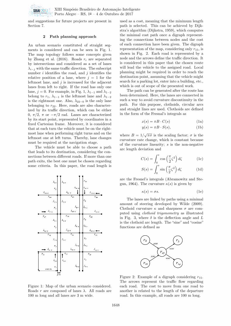
An urban scenario constituted of straight seg-ments is considered and can be seen in Fig. 1.The map topology follows some concepts givenby Zhang et al. (2016). Roads ri are separatedby intersections and considered as a set of lanesλi−j with the same traffic direction. The subscriptnumber i identifies the road, and j identifies therelative position of a lane, where j = 1 for theleftmost lane, and j is increased for the adjacentlanes from left to right. If the road has only onelane, j = 0. For example, in Fig. 1, λ1−1 and λ1−2belong to r1, λ1−1 is the leftmost lane and λ1−2is the rightmost one. Also, λ22−0 is the only lanebelonging to r22. Here, roads are also character-ized by its traffic direction, which can be either0, π/2, π or −π/2 rad. Lanes are characterizedby its start point, represented by coordinates in afixed Cartesian frame. Moreover, it is consideredthat at each turn the vehicle must be on the right-most lane when performing right turns and on theleftmost one at left turns. Thereby, lane changesmust be required at the navigation stage.

The vehicle must be able to choose a paththat leads to its destination, considering the con-nections between different roads. If more than onepath exits, the best one must be chosen regardingsome criteria. In this paper, the road length is

Figure 1: Map of the urban scenario considered.Roads r are composed of lanes λ. All roads are100 m long and all lanes are 3 m wide.

used as a cost, meaning that the minimum lengthpath is selected. This can be achieved by Dijk-stra’s algorithm (Dijkstra, 1959), which computesthe minimal cost path once a digraph represent-ing the connections between nodes and the costof each connection have been given. The digraphrepresentation of the map, considering only r15, isshown in Fig. 2. Each road is represented by anode and the arrows define the traffic direction. Itis considered in this paper that the chosen routewill lead the vehicle to the assigned road. Localplanning might be required in order to reach thedestination point, assuming that the vehicle mightsearch for a parking lot, enter into a building, etc.,which is out of scope of the presented work.

The path can be generated after the route hasbeen determined. Here, the lanes are connected insuch a way to avoid curvature discontinuity in thepath. For this purpose, clothoids, circular arcsand straight lines are used. Clothoids are definedin the form of the Fresnal’s integrals as

x(s) = πB · C(s) (1a)

y(s) = πB · S(s), (1b)

where B = 1/√πσ is the scaling factor; σ is the

curvature rate change, which is constant becauseof the curvature linearity; s is the non-negativearc length deviation and

C(s) =

∫ s

0

cos(π

2ζ2)dζ (1c)

S(s) =

∫ s

0

sin(π

2ζ2)dζ (1d)

are the Fresnel’s integrals (Abramowitz and Ste-gun, 1964). The curvature κ(s) is given by

κ(s) = σs. (1e)

The lanes are linked by paths using a minimalamount of steering developed by Wilde (2009).Clothoid curvature κ and sharpness σ are com-puted using clothoid trigonometry as illustratedin Fig. 3, where δ is the deflection angle and Lis the clothoid arc length. The “sine” and “cosine”functions are defined as

Figure 2: Example of a digraph considering r15.The arrows represent the traffic flow regardingeach road. The cost to move from one road toanother is related to the length of the departureroad. In this example, all roads are 100 m long.



1648

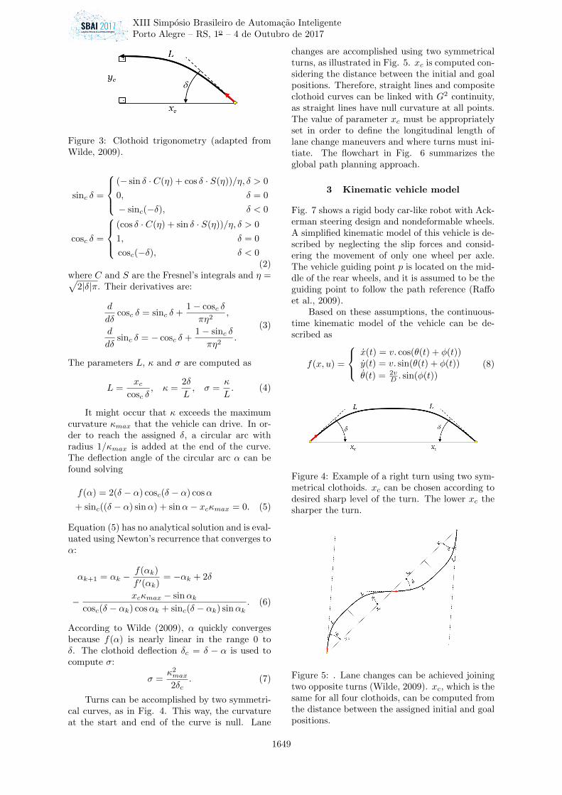
Figure 3: Clothoid trigonometry (adapted fromWilde, 2009).

sinc δ =

(− sin δ · C(η) + cos δ · S(η))/η,

0,

− sinc(−δ),

δ > 0

δ = 0

δ < 0

cosc δ =

(cos δ · C(η) + sin δ · S(η))/η,

1,

cosc(−δ),

δ > 0

δ = 0

δ < 0(2)

where C and S are the Fresnel’s integrals and η =√2|δ|π. Their derivatives are:

d

dδcosc δ = sinc δ +

1− cosc δ

πη2,

d

dδsinc δ = − cosc δ +

1− sinc δ

πη2.

(3)

The parameters L, κ and σ are computed as

L =xc

cosc δ, κ =

2δ

L, σ =

κ

L. (4)

It might occur that κ exceeds the maximumcurvature κmax that the vehicle can drive. In or-der to reach the assigned δ, a circular arc withradius 1/κmax is added at the end of the curve.The deflection angle of the circular arc α can befound solving

f(α) = 2(δ − α) cosc(δ − α) cosα

+ sinc((δ − α) sinα) + sinα− xcκmax = 0. (5)

Equation (5) has no analytical solution and is eval-uated using Newton’s recurrence that converges toα:

αk+1 = αk −f(αk)

f ′(αk)= −αk + 2δ

− xcκmax − sinαk

cosc(δ − αk) cosαk + sinc(δ − αk) sinαk. (6)

According to Wilde (2009), α quickly convergesbecause f(α) is nearly linear in the range 0 toδ. The clothoid deflection δc = δ − α is used tocompute σ:

σ =κ2max

2δc. (7)

Turns can be accomplished by two symmetri-cal curves, as in Fig. 4. This way, the curvatureat the start and end of the curve is null. Lane

changes are accomplished using two symmetricalturns, as illustrated in Fig. 5. xc is computed con-sidering the distance between the initial and goalpositions. Therefore, straight lines and compositeclothoid curves can be linked with G2 continuity,as straight lines have null curvature at all points.The value of parameter xc must be appropriatelyset in order to define the longitudinal length oflane change maneuvers and where turns must ini-tiate. The flowchart in Fig. 6 summarizes theglobal path planning approach.

3 Kinematic vehicle model

Fig. 7 shows a rigid body car-like robot with Ack-erman steering design and nondeformable wheels.A simplified kinematic model of this vehicle is de-scribed by neglecting the slip forces and consid-ering the movement of only one wheel per axle.The vehicle guiding point p is located on the mid-dle of the rear wheels, and it is assumed to be theguiding point to follow the path reference (Raffoet al., 2009).

Based on these assumptions, the continuous-time kinematic model of the vehicle can be de-scribed as

f(x, u) =

x(t) = v. cos(θ(t) + φ(t))y(t) = v. sin(θ(t) + φ(t))

θ(t) = 2vD . sin(φ(t))

(8)

Figure 4: Example of a right turn using two sym-metrical clothoids. xc can be chosen according todesired sharp level of the turn. The lower xc thesharper the turn.

Figure 5: . Lane changes can be achieved joiningtwo opposite turns (Wilde, 2009). xc, which is thesame for all four clothoids, can be computed fromthe distance between the assigned initial and goalpositions.



1649

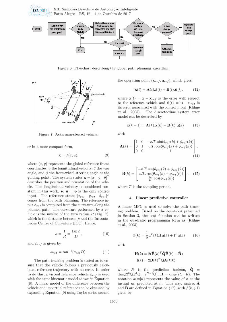
Figure 6: Flowchart describing the global path planning algorithm.

Figure 7: Ackerman-steered vehicle.

or in a more compact form,

x = f(x, u), (9)

where (x, y) represents the global reference framecoordinates, v the longitudinal velocity, θ the yawangle, and φ the front-wheel steering angle at theguiding point. The system states x = [x y θ]T

describes the position and orientation of the vehi-cle. The longitudinal velocity is considered con-stant in this work, so u = φ is the only controlinput. The reference states [xref yref θref ]T

comes from the path planning. The reference in-put φref is computed from the curvature along theplanned path. The curvature performed by a ve-hicle is the inverse of the turn radius R (Fig. 7),which is the distance between p and the Instanta-neous Center of Curvature (ICC). Hence,

κ =1

R=

tanφ

D, (10)

and φref is given by

φref = tan−1(κrefD). (11)

The path tracking problem is stated as to en-sure that the vehicle follows a previously calcu-lated reference trajectory with no error. In orderto do this, a virtual reference vehicle xref is usedwith the same kinematic model shown in Equation(8). A linear model of the difference between thevehicle and its virtual reference can be obtained byexpanding Equation (9) using Taylor series around

the operating point (xref ,uref ), which gives

˙x(t) = A(t).x(t) + B(t).u(t), (12)

where x(t) = x − xref is the error with respectto the reference vehicle and u(t) = u − uref isits error associated with the control input (Kuhneet al., 2005). The discrete-time system errormodel can be described by

x(k + 1) = A(k).x(k) + B(k).u(k) (13)

with

A(k) =

1 0 −v.T. sin(θref (k) + φref (k))0 1 v.T. cos(θref (k) + φref (k))0 0 1

,(14)

B(k) =

−v.T. sin(θref (k) + φref (k))v.T. cos(θref (k) + φref (k))

2vD . cos(φref (k))

, (15)

where T is the sampling period.

4 Linear predictive controller

A linear MPC is used to solve the path track-ing problem. Based on the equations presentedin Section 3, the cost function can be writtenin the quadratic programming form as (Kuhneet al., 2005)

Φ(k) =1

2uT (k)Hu(k) + fT u(k) (16)

with

H(k) = 2(B(k)T QB(k) + R)

f(k) = 2B(k)T QA(k|k)

where N is the prediction horizon, Q =diag(20Q,21Q,...2N−1Q), R = diag(R, ...R). Thenotation a(m|n) represents the value of a at theinstant m, predicted at n. This way, matrix Aand B are defined in Equation (17), with β(k, j, l)given by



1650

A(k) =

A(k|k)

A(k + 1|k)A(k|k)...

β(k, 2, 0)β(k, 1, 0)

B =

B(k|k) 0 · · · 0

A(k + 1|k)B(k|k) B(k|k) · · · 0...

.... . .

...β(k, 2, 1)B(k|k) β(k, 2, 2)B(k + 1|k) · · · 0β(k, 1, 1)B(k|k) β(k, 1, 2)B(k + 1|k) · · · B(k +N − 1|k)

(17)

β(k, j, l) =

l∏i=N−j

A(k + i|k). (18)

The term u is defined as

u(k) =

u(k|k)

u(k + 1|k)...

u(k +N − 1|k)

(19)

Matrix H(k) is an Hessian matrix. It is re-sponsible to describe the quadratic part of the costfunction, while f describes the linear part.

The optimization problem is solved at eachsampling time with the MATLAB routine quad-prog, and can be represented by

u∗ = argminu{Φ(k)}. (20)

There is an amplitude constraint in the con-trol variable u, described as

Zu(k + j|k) ≤ z, j ∈ [0, N − 1]

where

Z =

[I−I

], z =

[umax − uref (k + j)umin + uref (k + j)

].

With the input control φ determined, R canbe computed using Equation 11 and the left wheelangle φl and right wheel angle φr are given by

φl = (π/2)− tan−1(R− l/2)

φr = (π/2)− tan−1(R+ l/2),(21)

where l is distance between both rear wheels.

5 Results

Considering the map in Fig. 1, the path planneris used to generate four different routes: r1 to r6;r17 to r13; r16 to r14 and r10 to r20. It is assumedthat the vehicle must initiate the turn 5 metersfrom the point connecting the two assigned lanes.Lane changes are performed considering a 15 me-ters longitudinal distance and |κmax| <= 0.2. Theplanned paths are shown in Fig. 8 and their cur-vatures in Fig. 9.

The MPC approach is applied using V-REP, avirtual robot experimentation platform (Rohmer

−150 −100 −50 0 50 100 150 200 2500

50

100

150

200

250

300

350

400

450

500

Abscissa Axis (m)

Ord

inate

Axis

(m

)

Path1

Path2

Path3

Path4

Figure 8: Examples of paths considering four dif-ferent assigned routes. Path 1: r1 to r6; path 2:r17 to r13; path 3: r16 to r14; path 4: r10 to r20.

et al., 2013). V-REP provides a remote Applica-tion Programming Interface (API) useful for algo-rithm implementation, which is used is this paperto implement the algorithms in MATLAB. V-REPalso provides a model using Ackerman steering ge-ometry, depicted in Fig. 10. The constructive as-pect of the vehicle model used in this paper areshown in Table 1.

A new route from r11 to r15 is chosen to gener-ate the path that must be tracked by the vehicle.

The prediction horizon is set to N = 5, theweighting matrices are set to Q = diag(300, 300,500) and R = 5000, and an amplitude constraintof of z = [0.2 − 0.2]T was imposed on the input.According to Fig. 9, at all intersections the vehi-cle must reach |κmax|. As the turn path length is

Table 1: Constructive features of the Ackermansteering geometry model used for simulation.

D(m) l(m) |κmax|(m−1)2.5772 1.5103 0.2



1651

0 50 100 150 200 250 300 350 400

−0.2

−0.15

−0.1

−0.05

0

0.05

0.1

0.15

0.2

Distance (m)

Cu

rva

ture

(m

−1)

κ1

κ2

κ3

κ4

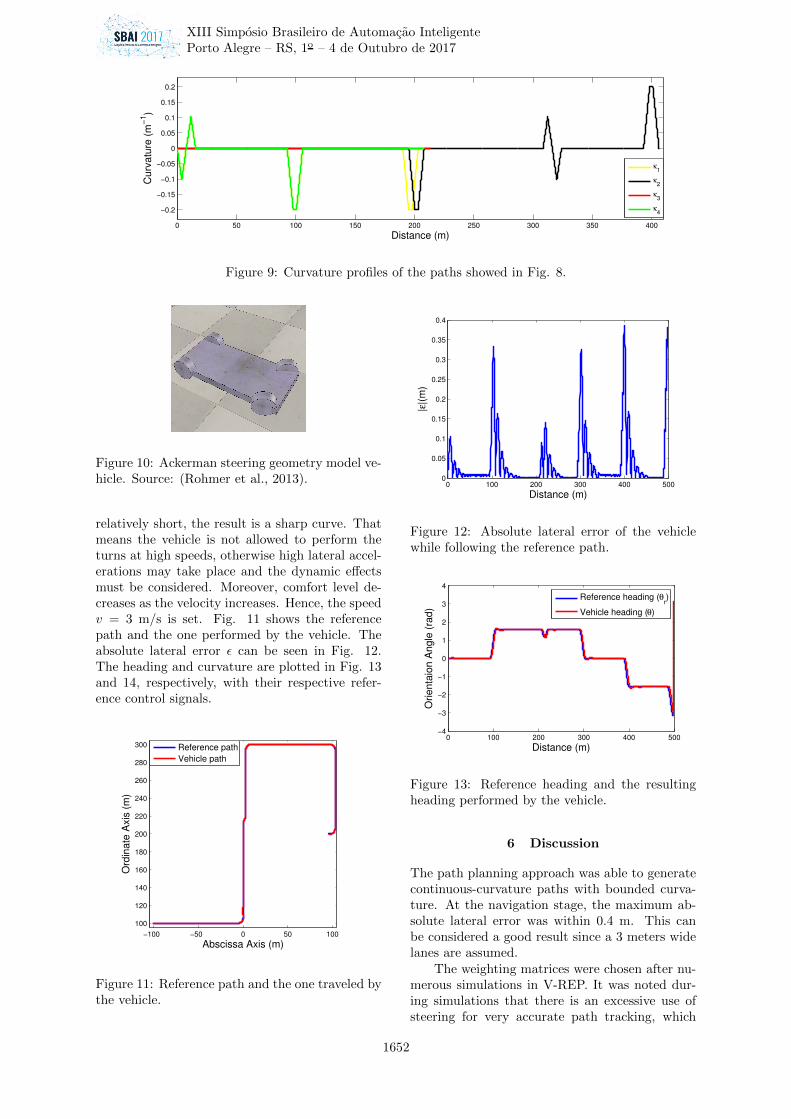
Figure 9: Curvature profiles of the paths showed in Fig. 8.

Figure 10: Ackerman steering geometry model ve-hicle. Source: (Rohmer et al., 2013).

relatively short, the result is a sharp curve. Thatmeans the vehicle is not allowed to perform theturns at high speeds, otherwise high lateral accel-erations may take place and the dynamic effectsmust be considered. Moreover, comfort level de-creases as the velocity increases. Hence, the speedv = 3 m/s is set. Fig. 11 shows the referencepath and the one performed by the vehicle. Theabsolute lateral error ε can be seen in Fig. 12.The heading and curvature are plotted in Fig. 13and 14, respectively, with their respective refer-ence control signals.

−100 −50 0 50 100

100

120

140

160

180

200

220

240

260

280

300

Abscissa Axis (m)

Ord

ina

te A

xis

(m

)

Reference path

Vehicle path

Figure 11: Reference path and the one traveled bythe vehicle.

0 100 200 300 400 5000

0.05

0.1

0.15

0.2

0.25

0.3

0.35

0.4

Distance (m)

|ε|(

m)

Figure 12: Absolute lateral error of the vehiclewhile following the reference path.

0 100 200 300 400 500−4

−3

−2

−1

0

1

2

3

4

Distance (m)

Orie

nta

ion

An

gle

(ra

d)

Reference heading (θr)

Vehicle heading (θ)

Figure 13: Reference heading and the resultingheading performed by the vehicle.

6 Discussion

The path planning approach was able to generatecontinuous-curvature paths with bounded curva-ture. At the navigation stage, the maximum ab-solute lateral error was within 0.4 m. This canbe considered a good result since a 3 meters widelanes are assumed.

The weighting matrices were chosen after nu-merous simulations in V-REP. It was noted dur-ing simulations that there is an excessive use ofsteering for very accurate path tracking, which



1652

0 100 200 300 400 500−0.25

−0.2

−0.15

−0.1

−0.05

0

0.05

0.1

0.15

0.2

0.25

Distance (m)

Cu

rva

ture

(m

−1)

Reference curvature (κr)

Vehicle curvature (κ)

Figure 14: Reference curvature and vehicle curva-ture while following the path.

may cause discomfort for passengers. Therefore,there is a trade-off between tracking accuracy andsmoothness.

7 Conclusion and future work

This paper presented a global path planning foran autonomous vehicle with Ackerman steeringgeometry in an urban scenario. The path was au-tomatically computed using information providedby a map. Turns and lane change maneuverswere performed using piecewise linear continuous-curvature paths, considering the maximum curva-ture that the vehicle can perform.

A model predictive control strategy was usedto solve the path tracking problem. The pro-posed controller was implemented using MATLABand simulated in V-REP environment using anAckerman-type vehicle model of its library. Onlythe kinematic model of the vehicle is considered inthis work. The results obtained were satisfactory,as the controller was able to maintain the vehiclewith a reasonable lateral error and reduced curva-ture rate change.

For future work, more complex scenarioscould be considered, where collision avoidance andlane merging will have to be taken into account.Moreover, the lateral forces acting on the vehi-cle can be included in the model so that the pathtracking controller may adjust the vehicle’s veloc-ity.

Acknowledgments

This work is supported by Coordination forthe Improvement of Higher Education Personnel(CAPES) under grants 1584685.

References

Abramowitz, M. and Stegun, I. A. (1964). Hand-book of mathematical functions: with formu-

las, graphs, and mathematical tables, Vol. 55,Courier Corporation.

Dijkstra, E. W. (1959). A note on two problemsin connexion with graphs, Numerische math-ematik 1(1): 269–271.

Fraichard, T. and Scheuer, A. (2004). From reedsand shepp’s to continuous-curvature paths,IEEE Transactions on Robotics 20(6): 1025–1035.

Korzeniowski, D. and Slaski, G. (2016). Methodof planning a reference trajectory of a sin-gle lane change manoeuver with bezier curve,IOP Conference Series: Materials Scienceand Engineering, Vol. 148, IOP Publishing,p. 012012.

Kuhne, F., Lages, W. F. and Silva, J. (2005).Mobile robot trajectory tracking using modelpredictive control, II IEEE latin-americanrobotics symposium.

Raffo, G. V., Gomes, G. K., Normey-Rico, J. E.,Kelber, C. R. and Becker, L. B. (2009). Apredictive controller for autonomous vehiclepath tracking, IEEE transactions on intelli-gent transportation systems 10(1): 92–102.

Rastelli, J. P., Lattarulo, R. and Nashashibi, F.(2014). Dynamic trajectory generation usingcontinuous-curvature algorithms for door todoor assistance vehicles, Intelligent VehiclesSymposium Proceedings, 2014 IEEE, IEEE,pp. 510–515.

Rohmer, E., Singh, S. P. and Freese, M. (2013).V-rep: A versatile and scalable robot simula-tion framework, Intelligent Robots and Sys-tems (IROS), 2013 IEEE/RSJ InternationalConference on, IEEE, pp. 1321–1326.

Shin, D. H. and Singh, S. (1990). Path generationfor robot vehicles using composite clothoidsegments, Technical report, DTIC Document.

Villagra, J., Milanes, V., Perez, J. and Godoy,J. (2012). Smooth path and speed plan-ning for an automated public transport ve-hicle, Robotics and Autonomous Systems60(2): 252–265.

Wilde, D. K. (2009). Computing clothoidsegments for trajectory generation, Intel-ligent Robots and Systems, 2009. IROS2009. IEEE/RSJ International Conferenceon, IEEE, pp. 2440–2445.

Zhang, T., Arrigoni, S., Garozzo, M., Yang, D.-g. and Cheli, F. (2016). A lane-level roadnetwork model with global continuity, Trans-portation Research Part C: Emerging Tech-nologies 71: 32–50.



1653

piecewise linear continuous-curvature path planning … · and suggestions for future projects are...

Documents