pid controllers for systems with timefor systems with time ... · pid controllers for systems with...

PID Controllers for Systems with Time-Delayfor Systems with Time Delay

1

PID Controllers for Systems with Time-Delay

General Considerations

CHARACTERISTIC EQUATIONS FOR DEALY SYSTEMS

Delay Tu(t)

y(t) = u(t¡ T )

Integratoru(t) y(t)_y(t)

Delay T

_y(t) + ay(t¡ T ) = u(t)

a

2


Delay T Integratoru(t) u(t¡ T )

y(t)_y(t)

_y(t) + ay(t) = u(t¡ T )

a

IntegratorDelay T_y(t) y(t)u(t)

IntegratorDelay T

a

_y(t) = ¡ay(t¡ T ) + u(t¡ T )

3


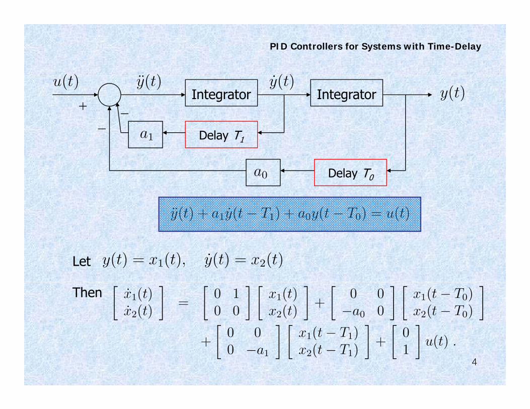
( ) _( )Ä( )Integrator Integrator

u(t)y(t)

_y(t)Äy(t)

Delay T1

Delay T0a0

a1

y 0

Äy(t) + a1 _y(t¡ T1) + a0y(t¡ T0) = u(t)

Let y(t) = x1(t); _y(t) = x2(t)

Then·

_x1(t)_x2(t)

¸=

·0 10 0

¸ ·x1(t)x2(t)

¸+

·0 0¡a0 0

¸ ·x1(t¡ T0)x2(t¡ T0)

¸·

0 0¸ ·

x1(t¡ T1)¸ ·

0¸

4

+

·0 00 ¡a1

¸ ·x1(t T1)x2(t¡ T1)

¸+

·01

¸u(t) :


St bilit f D l S tStability of Delay Systems

• Let y(t)=est be a proposed solution of

Ä(t) + _(t T ) + (t T ) 0y(t) + a1y(t¡ T1) + a0y(t¡ T0) = 0

• Then we have¡s2 + a1e

¡sT1s + a0e¡sT0

¢est ´ 0

¡ ¢so that “s” must satisfy s2 + a1se

¡sT1 + a0e¡sT0 = 0

Characteristic equation of the delay system.

The location of its zeros determine the stability of the system• The location of its zeros determine the stability of the system.

• If any roots lie in the closed RHP, the system is unstable as the solution grows without bound

5

solution grows without bound.


• Consider a LTI system with ℓ distinct delays,

_x(t) = A0x(t) +lX

Aix(t¡ Ti) + Bu(t)i=1

• The corresponding characteristic equation isÃl

!m

±(s) := det

ÃsI ¡ A0 ¡

lXi=1

e¡sTiAi

!= P0(s) +

mXk=1

Pk(s)e¡Lks

dn¡1 n¡1

and P0(s) = sn +Xi=0

aisi; Pk(s) =

Xi=0

(bk)isi

• (Retarded Delay Systems)• (Retarded Delay Systems)

• (Neutral Delay System)

Äy(t) + a1 _y(t¡ T1) + a0y(t¡ T0) = u(t)

6

(Neutral Delay System)Äy(t¡ T2) + a1 _y(t¡ T1) + a0y(t¡ T0) = u(t)


R t f Ch t i ti E tiRoots of Characteristic Equations

• Retarded Systems: There can only be a finite number of RHP roots. The stability of retarded systems is equivalent to the absence of closed RHP roots.

• The fact that retarded systems have a finite number of RHP t th t t th b f t iroots means that one can count the number of roots crossing

into the RHP through the stability boundary and keep track of the number of RHP roots as some parameter vary.

• Neutral Systems: Certain root chains can approach the imaginary axis from the LHP and thus destroy stability.

• If delays are multiples of a common delay, we have

±(s) = a0(s) + a1(s)e¡¿s + a2(s)e

¡2¿s + ¢ ¢ ¢+ ak(s)e¡k¿s

7

±(s) a0(s) + a1(s)e + a2(s)e + + ak(s)e


THE PADE APPROXIMATION AND ITS LIMITATIONS

e¡sL »= Nr(sL)

Dr(sL)where

Nr(sL) =rX

k=0

(2r ¡ k)!

k!(r ¡ k)!(¡sL)k

r(2 k)!

Dr(sL)Dr(sL) =

rXk=0

(2r ¡ k)!

k!(r ¡ k)!(sL)k

For example, the 3rd order Pade approximation is given by

N3(sL)

D3(sL)=¡L3s3 + 12L2s2 ¡ 60Ls + 120

L3s3 + 12L2s2 + 60Ls + 120

8


PID St bili ti f D l S t U i 1st O d P dPID Stabilization of a Delay Systems Using a 1st Order PadeApproximation (An Example)

• 1st Order Pade approximation ¡sL » 2¡ Ls• 1st Order Pade approximation e sL »=

2 + Ls

Pl t G( )

·k

¸¡sL »

·k

¸μ(¡Ls + 2)

¶• Plant G(s) =

·Ts + 1

¸e sL »=

·(Ts + 1)

¸μ( )

(Ls + 2)

¶

• With the PID controller (kp,ki,kd), the closed-loop characteristic polynomial becomes

±(s k ki kd) = s(Ts + 1)(Ls + 2) + (ki + k s + kds2)(k)(¡Ls + 2)±(s; kp; ki; kd) = s(Ts + 1)(Ls + 2) + (ki + kps + kds )(k)(¡Ls + 2)

= (Ts2 + s)(Ls + 2) + (k0ds2 + k0i)(¡Ls + 2) + k0ps(¡Ls + 2)

where k0d = kkd; k0i = kki; k

0p = kkp:

9

p


U i th PID D i Al ith h• Using the PID Design Algorithm, we have8>>>< ki > 0

ki ¡·

4(1 + kkp)¸

kd <2(1 + kkp)(2T + L¡ kkpL)<>>>:

ki

·L(4T + L¡ kkpL)

¸kd <

kL(4T + L¡ kkpL)

kd <T

kand

¡1

k< kp <

1

k

μ1 +

4T

L

¶

For a fixed kp, it becomes the set of linear inequalities in terms pof ki, kd and can be solved by LP.

10


Question: Does the 1st order Pade1 order Padeapproximation accurately capture the actual set of stabilizing PID parameters for the original time-delay system?

The stabilizing set of (ki,kd) values for a fixed kp. Next Example

11


E lExample

• Plant G(s) =

·1:6667

1 + 2 9036s

¸e¡0:2475s

·1 + 2:9036s

¸

• Plant with the 1st order Pade approximation

Gm(s) =1:6667

(1 + 2 9036s)

(¡0:1238s + 1)

(0 1238s + 1)(1 + 2:9036s) (0:1238s + 1)

Compute the entire stabilizing PID parameter values• Compute the entire stabilizing PID parameter values.

12


kp = 8:4467Time-response of the closed-loop systemp 8 67

ki = 60

kd = 1:5

closed loop system

The stabilizing (ki,kd) values at kp=8.4467

13

Showing unstable behavior!


• Tried with the 2nd, 3rd, and 5th order Pade approximation

• While the 2nd order Pade approximation fails to capture the actual stabilizing set, the 3rd and 5th order Pade

14

g ,approximations apparently do a better job.


Example with large delay

• Plant G(s) =

·1

1 + s

¸e¡10s

• Approximate the time-delay term using the 1st, 2nd, 3rd, 5th, 7th, and 9th order Pade approximations

15

1st and 2nd order approximations 3rd, 5th, 7th, and 9th order approximations


• For small values of the time-delay the approximate sets easily

Observations

• For small values of the time delay, the approximate sets easily converge to the possible true sets. However, the convergence becomes more difficult as the value of the time-delay increases.

The convergence of the approximate set to a possible true set• The convergence of the approximate set to a possible true set improves with increased order of the Pade approximation.

• The Pade approximation is not a satisfactory tool for ensuring the stability of the resulting control design.

It i t i i l t h t d f th i ti ill• It is not a priori clear as to what order of the approximation will yield a stabilizing set of parameters accurately approximating the true set.

16


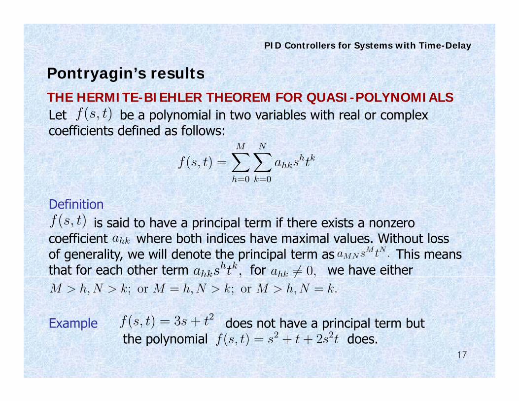
Pontryagin’s resultsTHE HERMITE-BIEHLER THEOREM FOR QUASI-POLYNOMIALSLet be a polynomial in two variables with real or complex f(s; t)

Pontryagin s results

coefficients defined as follows:

f(s; t) =MX NX

ahkshtk

h=0 k=0

Definitionis said to have a principal term if there exists a nonzerof(s; t) is said to have a principal term if there exists a nonzero

coefficient where both indices have maximal values. Without loss of generality, we will denote the principal term as This means that for each other term for we have either

f( ; )ahk

aMNsM tN :

ahkshtk; ahk 6= 0;

Example does not have a principal term but

hk ; hk 6 ;

M > h;N > k; or M = h;N > k; or M > h;N = k:

f(s; t) = 3s + t2

17

Example does not have a principal term but the polynomial does.f( ; )

f(s; t) = s2 + t + 2s2t


Theorem (Pontryagin)

If the polynomial does not have a principal term, then the function has an infinite number of zeros with arbitrarily

f(s; t)F (s) = f(s; es) y

large positive real parts.( ) f( ; )

If does have a principal term, the main result of Pontryagin is to show that the Hermite-Biehler Theorem extends

f(s; t)

to the class of functions F (s) = f(s; es):

18


Study of the zeros of functions of the form g(s,cos(s),sin(s))

• Let g(s,u,v) be a polynomial with real coefficients:M N

g(s; u; v) =MX

h=0

NXk=0

shÁ(k)h (u; v)

Á(k)

(u v) i l i l f d k h i dÁ( )h (u; v) is a polynomial of degree k, homogeneous in u and v.

• Assume that Á(k)h (u; v) is not divisible by u2 + v2 :Assume that Áh (u; v) is not divisible by u + v :

Á(k)h (1;§j) 6= 0

• Let Á¤(N)(u; v) =NX

k=0

Á(k)M (u; v) the coefficient of sM

19


• Consider G(s) = g(s; cos(s); sin(s))

• Let ©¤(N)(s) := Á¤(N)(cos(s); sin(s))( ) Á ( ( ); ( ))

THEOREM

L t ( ) b l i l ith i i l t i b sMÁ(N)

(u v)Let g(s,u,v) be a polynomial with principal term given by If η is such that does not take the value zero for real ω, then starting from some sufficiently large value of the function G(s)will have exactly zeros in the strip

s Á( )M (u;v):

©¤(N)(´ + j!)

4lN + M

l;will have exactly zeros in the strip

¡2l¼ + ´ · Re[s] · 2l¼ + ´:

Thus for the function G(s) to have only real roots it is necessary and

4lN + M

Thus for the function G(s) to have only real roots, it is necessary and sufficient that in the interval

¡2l¼ + ´ · Re[s] · 2l¼ + ´;

it h tl l t t ti ith ffi i tl l l

20

it has exactly real roots starting with some sufficiently large 4lN + M l:


• Consider

f(s; t) =MX

h=0

NXk=0

ahkshtk = sMX¤(N)(t) +

M¡1Xh=0

NXk=0

ahkshtk

X¤(N)(t) =NX

aMktk

Xk=0

Definition

L t h f( t) i l i l ith i i l tF ( ) f( s)Let where f(s,t) is a polynomial with a principal term, and F (j!) = Fr(!) + jFi(!)

Let ωr1, ωr2, ωr3, … denote the real roots of Fr(ω), and let ωi1, ωi2, ωi3,

F (s) = f(s; es):

… denote the real roots of Fi(ω), both arranged in ascending order of magnitude. The we say that the roots of Fr(ω) and Fi(ω) interlace if they satisfy the following property:

21

!r1 < !i1 < !r2 < !i2 < ¢ ¢ ¢


THEOREM (HB Theorem to quasi-polynomial)THEOREM (HB Theorem to quasi-polynomial)

If all the roots of F(s) lie in the open LHP, then the roots of Fr(ω)and Fi(ω) are real, simple, interlacing, and

0 0F

0i (!)Fr(!)¡ Fi(!)F

0r(!) > 0 (¤)

for each ω (-∞,∞), where Fr’(ω) and Fi

’(ω) denote the first derivative with respect to ω of Fr(ω) and Fi(ω), respectively. r iMoreover, in order that all the roots of F(s) lie in the open LHP, it is sufficient that one of the following conditions be satisfied:

1 All the roots of F (ω) and F (ω) are real simple and interlacing1. All the roots of Fr(ω) and Fi(ω) are real, simple, and interlacing and the inequality (*) is satisfied for at least one value of ω;

2. All the roots of Fr(ω) are real and for each root , (*) is satisfied, i.e.,

3. All the roots of Fi(ω) are real and for each root, (*) is satisfied, i.e.,

Fi(!r)F0r(!r) < 0;

F0i (!i)Fr(!i) > 0:

22

, i ( ) ( )


THEOREM

If the function has roots in the open RHP, then the function F(s) has an unbounded set of zeros in the open RHP. If all the zeros of the function lie in the open LHP,

X¤(N)(es)

X¤(N)(es) p ,then the function F(s) can only have a bounded set of zeros in the open RHP.

23


Application to Control Theory

Classes of Quasi-polynomials:

Retarded-type (or delay-type) Quasi-polynomials: This class consists of quasi-polynomials whose asymptotic chains go deep into the open LHP.

Neutral-type quasi-polynomials: This class consists of quasi-polynomials that along with delay-type chains contain at least one asymptotic chain of roots in a vertical strip of the complex plane.y p p p p

Forestall-type quasi-polynomials: This class consists of quasi-polynomials with at least one asymptotic chain that goes deep into the open RHPthe open RHP.

24


DefinitionA delay-type quasi-polynomial is said to be stable iff all its roots have negative real partshave negative real parts.

DefinitionA neutral-type quasi-polynomial is said to be stable if there exists a positive number σ such that the real parts of all its roots are less than –σ.

25


THEOREM

Let ±¤(s) = esLmd(s) + es(Lm¡L1)n1(s) + es(Lm¡L2)n2(s) + ¢ ¢ ¢+ nm(s)

and write Under the following conditions±¤(j!) = ±r(!) + j±i(!):

(A1) deg[d(s)] = q and deg[ni(s)] · q for i = 1; 2; :::;m;

(A2) 0 < L1 < L2 < ¢ ¢ ¢ < Lm

is stable iff±¤(s)( )

1. and have only simple, real roots and these interlace,

2.

±r(!) ±i(!)

±0i(!o)±r(!o)¡ ±i(!o)±

0r(!o) > 0; for some !o 2 (¡1;1):

26


E lExample

• Plant G(s) =1

2s + 1; C(s) = kp +

ki

s=

kps + ki

s2s + 1 s s

• With kp=1.8, ki=0.2, we have and it is stable.

±(s) = 2s2 + 2:8s + 0:2stable.

• Consider G(s) =

·1

2s + 1

¸e¡10s

·2s + 1

¸• With kp=1.8 and ki=0.2, the characteristic equation of the

closed-loop system is:c osed oop syste s±(s) = 2s2 + s + (1:8s + 0:2)e¡10s = 0

• For analyzing the stability, consider

27

±¤(s) = e10s±(s) = (2s2 + s)e10s + 1:8s + 0:2


• The real and imaginary parts are given by

±r(!) = 0:2¡ ! sin(10!)¡ 2!2 cos(10!)

( ) [ ( ) ( )]±i(!) = ![1:8 + cos(10!)¡ 2! sin(10!)] :

Shows interlacing Shows instability

28

Shows interlacing. Shows instability


Analysis

1. The example illustrates the case of a time-delay system that satisfies the interlacing and monotonic phase increase properties but fails to be stable.but fails to be stable.

2. The reason for this behavior lies in the nature of the roots of real and imaginary parts of the polynomial: they are not all real.

THEOREM (Pontyagin)

Let M and N denote the highest powers of s and es, respectively, inLet M and N denote the highest powers of s and e , respectively, in δ*(s). Let η be an appropriate constant such that the coefficients of terms of highest degree in δr(ω) and δi(ω) do not vanish at ω=η. Then for the equations δr(ω)=0 or δi(ω)=0 to have only real roots, q r( ) i( ) y ,it is necessary and sufficient that in each of the intervals

¡2l¼ + ´ · ! · 2l¼ + ´ l = lo; lo + 1; lo + 2; ¢ ¢ ¢δ (ω) or δ (ω) have exactly real roots for a sufficiently large4lN + M l

29

δr(ω) or δi(ω) have exactly real roots for a sufficiently large4lN + M l0:


• Let s = 10s

±¤(s) = (0:02s2 + 0:1s)es + 0:18s + 0:2

• The real and imaginary parts of the new quasi-polynomial is

±r(!) = 0:2¡ 0:1! sin(!)¡ 0:02!2 cos(!)( ) ( ) ( )

±i(!) = ![0:18 + 0:1 cos(!)¡ 0:02! sin(!)] :

• The roots of ±i(!) = 0( )

!o = 0; !1 = 8:0812; !2 = 8:8519; !3 = 13:5896; !4 = 15:4332;

!5 = 19:5618; !6 = 21:8025; ¢ ¢ ¢

• Choose ´ =¼

4

30


1 h l l t i [0± (^)1. has only one real root in [0, 2π-π/4]; the root at the origin.

2. Since is an odd function, in th i t l [ 7 /4 7 /4]

±i(!)

±i(!)± (^)the interval [-7π/4, 7π/4] ,

will have only one real root.

3. has no real roots in the interval [7π/4 9π/4];

±i(!)

±i(!)

^ ( )interval [7π/4, 9π/4]; has only one real root in [-2π+π/4, 2π+π/4] which does not sum up to

4N + M = 6 for l0 = 1:

±i(!)

4N + M 6 for l0 1:

4. Let so the requirement on the number if real roots is 8N+M=10. has only five real roots in [-4π+π/4, 4π+π/4].

l0 = 2 ±i(!)

has only five real roots in [ 4π+π/4, 4π+π/4].

5. Following the same procedure for we see that the number of real roots of in [-2 π+π/4, 2 π+π/4] is always less than

6 W l d h h f ll l

l = 3; 4; :::

l±i(!) l 4lN + M = 4l + 2:

± ( )

31

6. We conclude that the roots of are not all real.±i(!)


STABILITY OF SYSTEMS WITH A SINGLE DELAY

• Consider the characteristic equation

±(s; L) = d(s) + n(s)e¡Ls = 0

• Problem: Determine the ranges of values of L for which all the roots of the characteristic equation lie in the LHP.

• A systematic procedure to analyze the behavior of the roots of th h t i ti l i l L i f 0 tthe characteristic polynomial as L increases from 0 to ∞.

32


Walton and Marshall’s ProcedureWalton and Marshall s Procedure

Step 1: Examine the stability at L=0.

Step 2: • Examine the behavior of the roots as increasing L from 0 to an infinitesimally small and positive.

• The number of roots changes from being finite to infinite. For an infinitesimally small L, the new roots must come in at infinity. Otherwise, e-Ls ≈1 and no new roots.y ,

• Determine where in complex plane these new roots arise.

• If deg[n(s)]<deg[d(s)], the roots ‘’s’’ is large iff e-Ls is large (i.e., Re[s]<0) New roots occur in the open LHP

• If deg[n(s)]=deg[d(s)], the location of the roots is determined by the sign of W(ω2) for large ω.

33

y g ( ) g


Step 3: • Examine potential crossing points on the imaginary axisStep 3: • Examine potential crossing points on the imaginary axis (we separately consider the case s=0)

• Consider½d(j!) + n(j!)e¡jL! = 0

d(¡j!) + n(¡j!)ejL! = 0d(j!)d(¡j!)¡ n(j!)n(¡j!) = 0

W(!2) := d(j!)d(¡j!)¡ n(j!)n(¡j!)

• If no positive roots of W(ω2)=0, then no values of L for which ±(j!; L) = 0

Remark

If deg[n(s)]<deg[d(s)] and W(ω2) has no positive real roots, then there is no change in stability:The system will be stable for all L≥0 if the system is stable at L=0.

34

The system will be stable for all L≥0 if the system is stable at L 0.The system will be unstable for all L≥0 if the system is unstable at L=0.


Case when s=0Case when s=0

In this case, we have only one equation

d(0) + n(0) = 0 ) d(0) + e¡L0n(0) = 0; for all ¯nite L( ) ( ) ( ) ( ) ;

The system is unstable for all values of L and for analysis this solution can be ignoredsolution can be ignored.

To find L,

d(j!) + n(j!)e¡jL! = 0 ) e¡jL! = ¡d(j!)

n(j!):= cos(L!)¡ j sin(L!)

Once we have found a value of L at which there is a root of the characteristic equation on the imaginary axis, we need to determine if the root crosses the imaginary axis and in which direction or if it g ymerely touches the imaginary axis.

35


Re

·ds

¸> 0 Re

·ds

¸< 0 Re

·ds

¸= 0Re

·dL

¸> 0

destabilizing

Re

·dL

¸< 0

stabilizing

Re

·dL

¸0

Necessary to consider high-order derivativesg

After some manipulations, we have

S = sgn£W 0(!2)

¤=

½¡1; destabilizing+1 stabilizing

g£

( )¤ ½

+1; stabilizing

36


Examplep

±(s; L) = s + 2e¡Ls

1. Examine δ(s,0)=s+2, so the system is stable for L=0.

2. Since deg[d(s)]=1>deg[n(s)]=0, we skip step 2.

3. From d(s)=s, n(s)=2, we have W(ω2)= ω2-4.

• W’(ω2)=1>0.

• Since S=sgn[W’(ω2)]=1, the root is destabilizing.

• The corresponding values of L are

8 ·j!

¸8>><>>:cos(L!) = Re

·¡j!

2

¸= 0

sin(L!) = Im

·¡j!

2

¸= 1

L = (4k + 1)¼

4; k = 0; 1; 2; ¢ ¢ ¢

37

: ·2

¸


At L /4 two roots of δ(s L) 0 cross from left to right• At L=π/4, two roots of δ(s,L)=0 cross from left to right of the imaginary axis.

• At L=5π/4, two more roots cross from left to right of the imaginary axis and so on.

ConclusionConclusionThe region of stability is 0 ≤ L< π/4

38


FIRST ORDER SYSTEMS WITH TIME-DELAYFIRST ORDER SYSTEMS WITH TIME DELAY

Plant: G(s) =

·k

1 + Ts

¸e¡Ls

·1 + Ts

¸

PID Controller: C(s) = kp +ki

s+ kds

Stability Conditions for Delay free Systems

Characteristic Polynomial without time-delay:±(s) = (T + kkd)s

2 + (1 + kkp)s + kki

Assuming k>0, we have½kp > ¡1

k; ki > 0; kd > ¡T

k

¾or

½kp < ¡1

k; ki < 0; kd < ¡T

k

¾39

½p

k k

¾ ½p

k k

¾


Characteristic Polynomial with time delay:Characteristic Polynomial with time-delay:

±(s) = (kki + kkps + kkds2)e¡Ls + (1 + Ts)s

WriteeLs±(s) = kki + kkps + kkds

2 + (1 + Ts)seLs =: ±¤(s)

Substituting s=jω,±¤(j!) = ±r(!) + j±i(!)

wherewhere

±r(!) = kki ¡ kkd!2 ¡ ! sin(L!)¡ T!2 cos(L!)

±i(!) = ! [kkp + cos(L!)¡ T! sin(L!)]( ) [ p ( ) ( )]

We now separately treat the two cases: open-loop stable and open-loop unstable plants.

40


Open loop Stable PlantOpen-loop Stable Plant

Plant: G(s) =

·k

1 + Ts

¸e¡Ls T>0 (for stable plants)

·1 + Ts

¸

±¤(j!) = ±r(!) + j±i(!)

±r(!) = kki ¡ kkd!2 ¡ ! sin(L!)¡ T!2 cos(L!)

±i(!) = ! [kkp + cos(L!)¡ T! sin(L!)]

• kp only affects δi ω .

• ki and kd affect δr ω .i a d d a ect δr ω

• Parameters appear affinely in δr ω and δi ω .

For stability δ ω and δ ω must have all real roots and these

41

For stability, δr ω and δi ω must have all real roots and these roots must interlace.


LLemma

The imaginary part of δ* jω has only simple real roots iff

1 1·T

¸where α1 is the solution of the equation

¡1

k< kp <

1

k

·T

L®1 sin(®1)¡ cos(®1)

¸

in the interval (0, π .tan(®) = ¡ T

T + L®

This lemma gives the ranges of kp.

42


L t L 0 thLet z=ωL≠0, then

±r(z) =k

L2z2 [¡kd + m(z)ki + b(z)]

where

m(z) =L2

z2; b(z) = ¡ L

kz

·sin(z) +

T

Lz cos(z)

¸· ¸LemmaFor each value of kp in the range, the necessary and sufficientFor each value of kp in the range, the necessary and sufficient conditions on ki and kd for the roots of δr(z) and δi(z) to interface is the following infinite set of inequalities:

ki > 0 kd > m1ki + b1 kd < m2ki + b2 kd > m3ki + b3

where the parameters mj and bj for j=1,2,3,… are given by

ki > 0; kd > m1ki + b1; kd < m2ki + b2; kd > m3ki + b3;

kd < m4ki + b4; ¢ ¢ ¢

43

mj := m(zj); bj := b(zj):


Theorem

The range of k values for which a given open-loop stable plant withThe range of kp values for which a given open loop stable plant, with transfer function considered, can be stabilized using a PID controller is given by

1 1·T

¸where α1 is the solution of the equation

¡1

k< kp <

1

k

·T

L®1 sin(®1)¡ cos(®1)

¸

in the interval 0,π . For kp values outside this range, there are no bili i PID ll Th l bili i i i i b

tan(®) = ¡ T

T + L®

stabilizing PID controllers. The complete stabilizing region is given by:

44

F h k /k /k


For each kp ‐1/k,1/k , the cross‐section of the stabilizing region in the k k space is theki,kd space is the trapezoid T;

For kp=1/k, the pcross-section of the stabilizing region in the (ki,kd) space is th t i l Δthe triangle Δ;

For each k 1/k k the cross‐mj =

L2

z2j

;

For each kp 1/k,ku , the crosssection of the stabilizing region in the ki,kd space is the quadrilateral Q.

bj = ¡ L

kzj

·sin(zj) +

T

Lzj cos(zj)

¸!j =

zj

kL

·sin(zj) +

T

Lzj(cos(zj) + 1)

¸45

kL

·L

¸where zj are the real, positive solutions of kkp + cos(z)¡ T

Lz sin(z) = 0


Algorithm for Determining Stabilizing PID ParametersAlgorithm for Determining Stabilizing PID Parameters

1. Initialize kp=-1/k and step=(ku+1/k)/(N+1) where N is the desired number of points and

2 S t K k t

ku =1

k

·T

L®1 sin(®1)¡ cos(®1)

¸2. Set Kp=kp+step;

3. If kp<ku, then go to 4. Else terminate the algorithm.

4 Find the roots z and z of4. Find the roots z1 and z2 of

kkp + cos(z)¡ T

Lz sin(z) = 0:

5. Compute the parameters mj and bj, j=1,2 associated with the zj.

6. Determine the stabilizing region in the (ki,kd) space.

L

46

g g ( i, d) p

7. Go to 2.


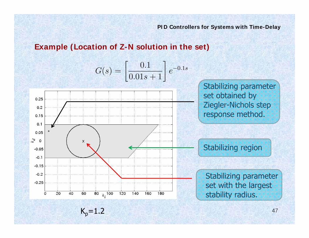
E l (L ti f Z N l ti i th t)Example (Location of Z-N solution in the set)

G(s) =

·0:1

0 01 1

¸e¡0:1s( )

·0:01s + 1

¸Stabilizing parameter set obtained by Ziegler Nichols stepZiegler-Nichols step response method.

Stabilizing region

Stabilizing parameter set with the largest stability radius

47Kp=1.2

stability radius.


E l (S t i P d A i ti S t iExample (Set using Pade Approximation vs. Set using a True Delay System)

Set from the true delay system3D stabilizing set

48

Set from the 1st order Pade approximation(It contains destabilizing parameters)


Open loop Unstable PlantOpen-loop Unstable Plant

Plant: G(s) =

·k

1 + Ts

¸e¡Ls T<0 (for unstable plants)

·1 + Ts

¸

Lemma

For |T/L|>0.5, δi jω) has only simple real roots iff

1

k

·T

L®1 sin(®1)¡ cos(®1)

¸< kp < ¡1

k

where α1 is the solution of the equation

k

·L

( ) ( )

¸p

k

tan(®) =T

®

in the interval (0,π . In the special case of |T/L|=1, we have α1 π/2. For |T/L|≤0 5 the roots of δ jω) are not all real

tan(®) = ¡T + L

®

49

For |T/L|≤0.5, the roots of δi jω) are not all real.


Let z=ωL≠0Let z=ωL≠0,

±r(z) =k

L2z2 [¡kd + m(z)ki + b(z)]

where m(z) =L2

z2; b(z) = ¡ L

kz

·sin(z) +

T

Lz cos(z)

¸LemmaFor each value of kp in the range, the necessary and sufficient conditions on ki and kd for the roots of δr(z) and δi(z) to interlace are the following infinite set of inequalities:

ki < 0; kd < m1ki + b1; k ¡ d > m2ki + b2; kd < m3ki + b3;

kd > m4ki + b4 ¢ ¢ ¢where the parameters mj and bj for j=1,2,3,… are given by

kd > m4ki + b4;

mj := m(zj); bj := b(zj)

50

j ( j); j ( j)


TheoremTheorem

A necessary and sufficient condition for the existence of a stabilizing PID controller for the open-loop unstable plant considered is |T/L| 0 5 If thi diti i ti fi d th th f k l|T/L|>0.5. If this condition is satisfied, then the range of kp values for which a given open-loop unstable plant, with transfer function considered, can be stabilized using a PID controller is given by

1·T

¸1


1

k

·T

L®1 sin(®1)¡ cos(®1)

¸< kp < ¡1

k


tan(®) = ¡ T

T + L®

in the interval (0,π). In the special case of |T/L|=1, we have α1 π/2. For kp values outside this range, there are no stabilizing PID controllers. Moreover, the complete stabilizing region is given:

51


For each kp kl,‐1/k , the cross‐section of the stabilizing region in thestabilizing region in the ki,kd space is quadrilateral Q.

The stabilizing region of (ki,kd) for kl<kp<-1/k where

kl :=1

k

·T

L®1 sin(®1)¡ cos(®1)

¸52

k

·L

¸


E lExample

dy(t)0 25y(t) 0 25u(t 0 8)

Consider a process defined by

G(s) =1

e¡0:8s( )

dt= 0:25y(t)¡ 0:25u(t¡ 0:8) G(s) =

1¡ 4se

The stabilizing region of (k k k ) l f h(kp,ki,kd) values for the PID controllers. (-8.6876<kp<-1)

53

ARBITRARY LTI SYSTEMS WITH A SINGLE


ARBITRARY LTI SYSTEMS WITH A SINGLE TIME-DELAY

Tsypkin proposed a method to extend the Nyquist criterion to dealTsypkin proposed a method to extend the Nyquist criterion to deal with time-delay systems (1946). This may lead to misleading conclusions unless care is taken.

Example G(s) =2s + 1

s + 2

• The closed-loop system is stable with unity negative feedback.

• According to Tsypkin, the closed-loop system should tolerateAccording to Tsypkin, the closed loop system should tolerate a time-delay upto 3.7851.

• However, when we add a 1 second delay to the nominal transfer function the closed-loop system becomes unstable

54

transfer function, the closed-loop system becomes unstable.


• The Nyquist plot intersects the unit circle at ω 1unit circle at ω0=1.

• The closed-loop system should tolerate a time-delay upto The closed-loop system is

unstable with a 1 second delay

55

L0 =¼ + arg G(j!0)

!0= 3:7851:

unstable with a 1 second delay.

Pontryagin’s Theory vs. the Nyquist Criterion


y g y yq

Let h(z,t) be a polynomial in the two variable z and t with constant coefficients,

h(z t) =X

a zmtnh(z; t) =Xm;n

amnz t

The term arszrts is called the principle term of the polynomial if ars≠0and r and s each attain their maximum.

Writeh(z; t) = Â(s)

r (t)zr + Â(s)r¡1(t)z

r¡1 + ¢ ¢ ¢+ Â(s)1 (t)z + Â

(s)0 (t);

where are polynomials in twith degree atÂ(s)j (t); j = 0; 1; 2; : : : ; rwhere are polynomials in twith degree at

most equal to s.Âj (t); j 0; 1; 2; : : : ; r

56


Two Theorems of Pontryagin to Clarify Nyquist CriterionTwo Theorems of Pontryagin to Clarify Nyquist Criterion Based Conditions for Systems with Time-delay

TheoremTheoremIf the polynomial has no principal term, then the function

h(z; t) =Xm;n

amnzmtn

has an unbounded number of zeros with arbitrary large positive real part.

H(z) = h(z; ez)

TheoremLet H(z)=h(z,ez) where h(z,t) is a polynomial with principal term arszrts. If the function χr s ez has roots in the open RHP, then the function H(z)has an unbounded set of zeros in the open RHP. If all the zeros of the function χr s ez lie in the open LHP, then the function H(z) has no

th b d d t f i th RHP

57

more than a bounded set of zeros in the open RHP.


C diti hi h h ld b ti fi d h i thConditions which should be satisfied when using the Nyquist criterion with the conventional Nyquist contour

TheoremSuppose that we are given a unity feedback system with an open-loop transfer function

G( ) G ( ) ¡Ls

·N(s)

¸¡Ls

where N(s) and D(s) are real polynomials of degree m and n, respectively and L is a fixed delay Then we have the following

G(s) = G0(s)eLs =

·( )

D(s)

¸e Ls

respectively and L is a fixed delay. Then we have the following conclusions:1. If n<m, or, n=m and |bn/an|≥1 where an, bn are the leading

coefficients of D(s) and N(s) respectively the Nyquist criterion is notcoefficients of D(s) and N(s), respectively, the Nyquist criterion is not applicable and the system is unstable according to Pontryagin’stheorems.

58

2. If n>m, or, n=m and |bn/an|<1, the Nyquist criterion is applicable and we can use it to check the stability of the closed-loop system.


It is appropriate to point out that most likely Typkin assumed the pp p p y ypplant to be strictly proper, though he did not state it explicitly in the literature. Attaching a PID controller to a proper or strictly proper plant opens up the very real possibility of ending up with an improper or a proper open-loop transfer function. This is the reason that the above investigation had to be undertaken.

59


Solution Approach

1. Find the complete set of k’s which stabilize the delay-free plant P0(s)and denote this set as S0.

2. Define the set SN, which is the set of k’s such that C(s,k)P0(s) is an2. Define the set SN, which is the set of k s such that C(s,k)P0(s) is an improper transfer function or

lims!1

jC(s;k)P0(s)j ¸ 1

Note that the elements in SN make the closed-loop system unstable after the delay is introduced. Exclude SN from S0 and denote the new set by S1, that is, S1 = S0nSN

3. Compute the set SL:

SL =©k j k 62 SN and 9L 2 [0; L0]; ! 2 R; s:t:C(j!)P0(j!)e¡jL! = ¡1

ªSL is the set of k’s which make C(s,k)P(s) have a minimal destabilizing delay that is less than or equal to L0.

4 The set is the solutionSR = S1nSL

60

4. The set is the solutionSR = S1nSL


TheoremTheoremThe set of controllers C(s,k) denoted by SR is the complete set of controllers in the unity feedback configuration that stabilize the plant P(s) with delay L from 0 up to L0.P(s) with delay L from 0 up to L0.

Proportional Controllers

Plant and controller: P (s) = P0(s)e¡Ls =

·N(s)

¸e¡Ls C(s) = kPlant and controller: P (s) = P0(s)e =

·D(s)

¸e ; C(s) = kp

To implement the method, the key is to find SL.

61


Th i t th N i t i ( 1 0) Fi d L d ti f iThe point the Nyquist curve crossing (-1,0): Find L and ω satisfying

C(j!)P0(j!)e¡jL! = ¡1

arg[kpP0(j!)]¡ L! = 2h¼ ¡ ¼; h 2 Z

jkpP0(j!)j = 1:

L(!; kp) =arg[kpP0(j!)] + ¼

!1

kp(!) = § 1

jP0(j!)j :

62


• For kp>0, L(!; kp) = L(!) =

arg[P0(j!)] + ¼

!

Solve L(ω)≤L0 to get a set of ω: ΩSet of kp>0 corresponding to Ω : SL

SL+ consists of all the positive kp’s that make the system have poles on the imaginary axis for certain L≤L0.

• For Kp<0,Ω‐ : a set of ω for L(ω)≤L0SL‐ : a set of kp<0 corresponding to Ω‐

The complete set S : SL = S+L [ S¡L

63

The complete set SL: SL SL [ SL


Algorithm for P Controllers

1. Compute the delay-free stabilizing kp set, S0

2 Fi d S2. Find SN

• If deg[N(s)]>deg[D(s)], SN=R. i.e., SR=

• If deg[N(s)]<deg[D(s)] S =• If deg[N(s)]<deg[D(s)], SN=

• If deg[N(s)]=deg[D(s)],

SN =

½k j jk j ¸

¯an

¯¾where an, bn are the leading coefficients of D(s) and N(s).

3 Compute

SN =

½kp j jkpj ¸

¯bn

¯¾;

S S nS3. Compute

4. Compute SL

5 Compute

S1 = S0nSN

SR = S1nSL

64

5. Compute SR = S1nSL


ExampleExample

P (s) =

·s2 + 3s¡ 2

s3 + 2s2 + 3s + 2

¸e¡Ls with delay up to L0 = 1:8

• For the delay-free plant, the stabilizing kp range g p gS0=(-0.4093,1).

• Since deg[N(s)]=2<deg[D(s)],deg[N(s)] 2<deg[D(s)], SN= and S1=S0

• For kp>0, Ω 1 5129 ∞Ω 1.5129, ∞

65


• The corresponding S + = [0 4473 +∞• The corresponding SL+ = [0.4473, +∞

66


For kp<0, Ω‐ 0.7359, p1.3312 2.6817, ∞

The corresponding SL‐0.6025, ‐0.4135 ,

‐∞, ‐1.3691

SR = S1nSL

( 0 4093 1)n([0 4473 ) [ 0 6025 0 4135] ( 1 3691])

67

= (¡0:4093; 1)n([0:4473; +1) [ [¡0:6025;¡0:4135] [ (¡1;¡1:3691])

= (¡0:4093; 0:4473)


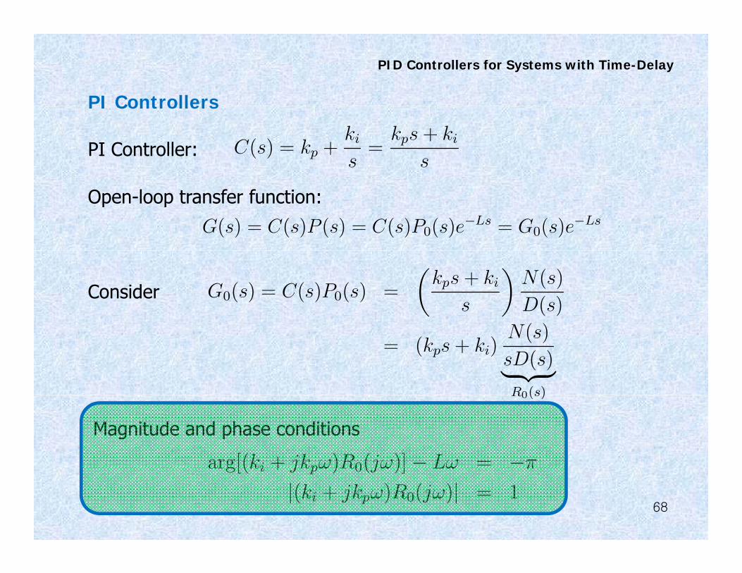
PI ControllersPI Controllers

PI Controller: C(s) = kp +ki

s=

kps + ki

s

Open-loop transfer function:

G(s) = C(s)P (s) = C(s)P0(s)e¡Ls = G0(s)e

¡Ls

Consider G0(s) = C(s)P0(s) =

μkps + ki

s

¶N(s)

D(s)

= (kps + ki)N(s)

sD(s)| z R0(s)R0(s)

Magnitude and phase conditions

arg[(ki + jkp!)R0(j!)]¡ L! = ¡¼

68

arg[(ki + jkp!)R0(j!)] L! ¼

j(ki + jkp!)R0(j!)j = 1


Rewrite the magnitude and phase conditionsRewrite the magnitude and phase conditions,

L(!; kp; ki) =arg[(ki + jkp!)R0(j!)] + ¼

!!

ki = §s

1

jR0(j!)j2 ¡ k2p!

2:

Fix kp, then

M(!) =1

jR0(j!)j2 ¡ k2p!

2ki = §

pM(!)

Note that only those ω’s with M(ω)≥0 need consideration when computing SL.

69


Algorithm for PI Controllers

1. Compute S0

2 C t S2. Compute SN

• If deg[N(s)]>deg[D(s)], SN=R2, i.e., SR=

• If deg[N(s)]<deg[D(s)] S =• If deg[N(s)]<deg[D(s)], SN=

• If deg[N(s)]=deg[D(s)],

where a , b are leading coefficients of D(s) and N(s).

SN =

½(kp; ki)jkp; ki 2 R and jkpj ¸

¯an

bn

¯¾where an, bn are leading coefficients of D(s) and N(s).

3. Compute

4. For a fixed kp, find SR,kp

S1 = S0nSN

p, R,kp

• Determine the sets Ω and

• Determine the sets Ω‐ and

S+L;kp

:

S¡L;kp:

70


5 Compute5. Compute

SL;kp = S+L;kp

[ S¡L;kp

SR;kp = S1;kpnSL;kp

6. By sweeping over kp, the complete set of PI controllers that

p p p

pstabilize all plant with delay up to L0

SR =[kp

SR;kp

kp

71


PID Controllers for an Arbitrary LTI Plant with DelayPID Controllers for an Arbitrary LTI Plant with Delay

G(s) = C(s)P0(s)e¡Ls = G0(s)e

¡Ls

wherewhere

G0(s) = C(s)P0(s) =kds

2 + kps + ki

s¢ N(s)

D(s)

2

·N(s)

¸= (kds

2 + kps + ki)

·N(s)

sD(s)

¸| z

R0(s)

The magnitude and phase conditions:

arg[(ki ¡ kd!2 + jkp!)R0(j!)]¡ L! = ¡¼

j(ki ¡ kd!2 + jkp!)R0(j!)j = 1

72


Rewrite the phase and magnitude conditions,Rewrite the phase and magnitude conditions,

L(!; kp; ki; kd) =¼ + arg ([(ki ¡ kd!

2) + jkp!] ¢R0(j!))

!

ki ¡ kd!2 = §

s1

jR0(j!)j2 ¡ (kp!)2:

For fixed kp,

M( )1

(k )2M(!) = jR0(j!)j2 ¡ (kp!)2 ki ¡ kd!2 = §

pM(!)

Similar to the PI case, we only need to consider ω’s with M(ω)≥0 when computing SL.

73


Algorithm for PID Controllers

1. Compute S0

2 C t S2. Compute SN

• If deg[N(s)]>deg[D(s)]-1, SN=R3, i.e., SR=

• If deg[N(s)]<deg[D(s)]-1 S =• If deg[N(s)]<deg[D(s)]-1, SN=

• If deg[N(s)]=deg[D(s)]-1,

S½

(k k k )jk k k 2 R d jk j ¸¯

an

¯¾where an, bn1 are leading coefficients of D(s) and N(s).

SN =

½(kp; ki; kd)jkp; ki; kd 2 R and jkdj ¸

¯ n

bn¡1

¯¾

n n 1 g ( ) ( )

3. Compute

4. For a fixed kp, determine the set SR,kp

S1 = S0nSN

74


• Determine the set Ω and SL k +Determine the set Ω and SL,kp

Ð+ =

½! j ! > 0 and M(!) ¸ 0 and

f[p

M( ) jk ] R (j )g ¾L(!) =

¼ + argf[p

M(!) + jkp!] ¢R0(j!)g!

· L0

¾S+

L k =

½(ki; kd) j (ki; kd) =2 SN;kp and 9 ! 2 Ð+

h f h l h (k k )

L;kp

½( i; d) j ( i; d) = N;kp

such that ki ¡ kd!2 =

pM(!)

¾:

Note that SL,kp+ is a set of straight lines in the (ki,kd) space.

• Determine the sets Ω‐ and SL,kp‐

Compute S S+ [ S¡ d S S nS• Compute

5. By sweeping over kp, the complete set of PID controllers that stabilize all plants with delay up to L0:

SL;kp = S+L;kp

[ SL;kpand SR;kp = S1;kpnSL;kp

75

SR =[kp

SR;kp


ExampleExample

P (s) =k

Ts + 1e¡Ls; L 2 [0; L0]

The stabilizing PID parameters for the delay-free plant are:

S0 =

½(kp; ki; kd) j kp > ¡1

k; ki > 0; kd > ¡T

kor kp < ¡1

k; ki < 0; kd < ¡T

k

¾½k k k k

¾

Since deg[D(s)]-deg[N(s)]=1,½ ¯T

¯¾SN =

½(kp; ki; kd) j kp; ki; kd 2 R and jkdj ¸

¯T

k

¯¾Assuming k>0 we haveAssuming k>0, we have

S1 = S0nSN =

8<:©(kp; ki; kd) j kp > ¡ 1

k; ki > 0; T

k> kd > ¡T

k

ªfor T > 0©

(k k k ) j k < 1 k < 0 T < k < Tª

for T < 0

76

: ©(kp; ki; kd) j kp < ¡ 1

k; ki < 0; T

k< kd < ¡T

k

ªfor T < 0


For T>0 with different k values the stabilizing regions of (k k ) takeFor T>0, with different kp values, the stabilizing regions of (ki,kd) take on different but simple shapes:

For -1/k<k ≤1/kFor 1/k<kp≤1/k, SR,kp is a trapezoid. (a)

For kp>1/k, SR,kp is a quadrilateral. (b) and (c)and (c)

77


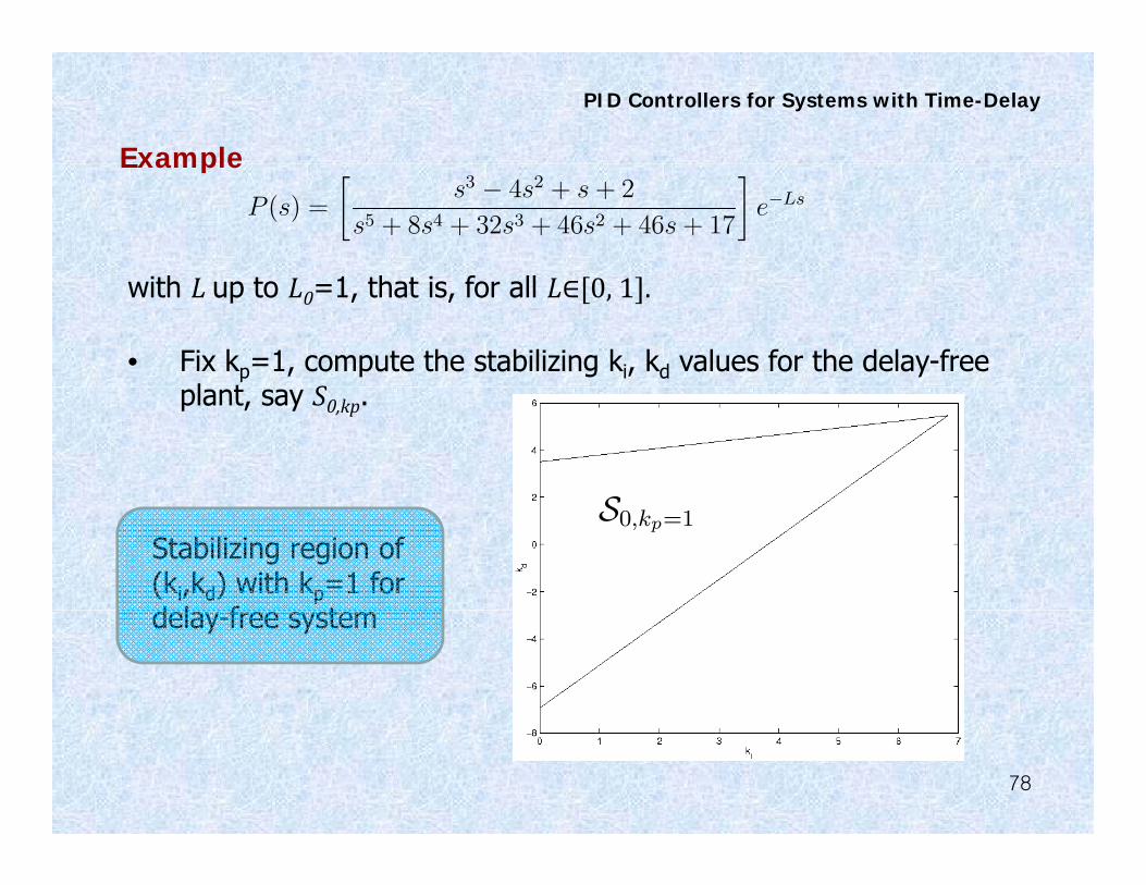
ExampleExample

P (s) =

·s3 ¡ 4s2 + s + 2

s5 + 8s4 + 32s3 + 46s2 + 46s + 17

¸e¡Ls

fwith L up to L0=1, that is, for all L 0, 1 .

• Fix kp=1, compute the stabilizing ki, kd values for the delay-free l t Splant, say S0,kp.

SStabilizing region of (ki,kd) with kp=1 for d l f t

S0;kp=1

delay-free system

78


Si d [ ( )] d [ ( )] 1 d• Since deg[D(s)]-deg[N(s)]>1, SN= and S1 S0.

• For the set of ω where L(ω)≤L0 is

Ω 0 524825 0 742302 2 57318 ∞

ki ¡ kd!2 =

pM(!) > 0;

Ω 0.524825, 0.742302 2.57318, ∞

79

L(ω) vs. ωwith ki ¡ kd!2 =

pM(!)


• The corresponding values ofp

M( )• The corresponding values of

• SL,kp+ : the straight lines defined by

pM(!)

ki ¡ kd!2 =

pM(!) for ! 2 Ð+ki kd! =

pM(!) for ! 2 Ð

p( )

80

pM(!) vs: ! with kp = 1


• For k k 2p

M( ) 0• For ki ¡ kd!2 = ¡

pM(!) < 0;

Ω- = [1.35894, 1.8659] 4.37326, ∞

81

L(!) vs: ! with ki ¡ kd!2 = ¡

pM(!)


Finally, we exclude SL k + and SL k – from S1 k to get SR kFinally, we exclude SL,kp and SL,kp from S1,kp to get SR,kp

Stabilizing region of (k k ) withof (ki, kd) with kp=1 for plant with delay up to 1.

82

pid controllers for systems with timefor systems with time ... · pid controllers for systems with...

Documents