arX

iv:0

706.

0366

v1 [

phys

ics.

pop-

ph]

4 J

un 2

007

On the Flight of the American Football

C. Horn and H. Fearn

Physics Department,

California State University Fullerton,

Fullerton CA 92834 USA.

email: curtishorn@alum.rpi.edu,

hfearn@fullerton.edu

(Dated: February 13, 2013)

Abstract

In this paper we examine the detailed theory of the American football in flight, with spin and air

resistance included. We find the theory has much in common with the theory of a gyroscope and also

rocket trajectory with a misaligned thruster. Unfortunately most of the air resistance data, for rocketry

and ballistics, is for speeds of Mach 1 or higher, where the air resistance increases dramatically. We

shall approximate a realistic air resistance, at the slower speeds of football flight, with a drag force

proportional to cross sectional area and either v or v2, depending on speed, where v is velocity of the

football. We begin with a discussion of the motion, giving as much detail as possible without the use

of complex analytic calculations. We point out the previous errors made with moments of inertia and

make the necessary corrections for more accurate results.

1

I. INTRODUCTION

It has come to our attention that there are still some unresolved problems relating to football

flight. Dr. Timothy Gay, author of a popular book on Football Physics1 suggested a challenge

at a recent meeting of the Division of Atomic, Molecular and Optical Physics, in Tennessee,

May 2006. The challenge given at the conference was to explain why the long axis of the

ball appears to turn (pitch) and follow the parabolic trajectory of the flight path. After an

extensive literature search we have found that the theory of why a football pitches in flight has

been explained quite well by Brancazio2. The more general theory of a football in flight, giving

elaborate mathematical details has been given by both Brancazio and Rae3,4,5. We have found

that the literature (especially comments found online) do tend to use improper moments of

inertia for the football and incorrectly apply the Magnus force (known as spin drift in ballistics)

to explain yaw of the football in flight. Clearly, since a challenge was posed by an expert in

football physics, we feel the need to summarize the literature in this area and update it where

necessary.

We intend to give the reader all the mathematical details needed for an accurate description

of the moments of inertia for the football. The needed theory, on torque free precessional

motion (for more than one spin axis) and gyroscopic motion when torque is applied, is already

available in standard mechanics texts6,7. With the use of these texts and papers like that of

Brancazio2,5 we take the theory to be well enough expounded. We will merely quote the needed

equations and cite the references.

The second author would also like to take this opportunity to write a paper on “something

typically American” to celebrate becoming an American citizen in June 2006.

Several scientists at SUNY; State University of New York at Buffalo, have an e-print online

with flight data taken with an onboard data recorder for an American football. They used a

“Nerf” ball and cut out the foam to incorporate circuit boards and four accelerometers inside the

ball8. They confirm that a typical spin rate is 10 rev/sec or 600 RPM (revolutions per minute)

from their data. They also give a precession frequency of 340 RPM which gives a 1.8 value for

2

the spin to precession rate ratio (spin to wobble ratio). We will discuss this further later on.

The usual physics description of football flight, of the kind you can find online, is at the

level of basic center of mass trajectory, nothing more complex than that9. It is our intention

in this article to go into somewhat greater detail in order to discuss air resistance, spin, pitch

and yaw. We find that the literature uses, for the most part, a bad description of the moments

of inertia of the football. We intend to remedy that. Our review will encompass all possible

flight trajectories, including kicking the ball and floating the ball. We will briefly review the

equations needed for all possible scenarios.

In order to conduct this analysis it will be necessary to make some basic assumptions. We

assume that solid footballs may be approximated by an ellipsoid, we ignore any effect of the

laces. We note that a Nerf ball (a foam ball with no laces) has a very similar flight pattern to

a regular inflated football, so the laces can be thought to have little or no effect, they just help

in putting the spin on the ball. More about this later. For game footballs we will consider a

prolate spheroid shell and a parabola of revolution for the shapes of the pigskin. We calculate

the moments of inertia (general details in Appendix A and B) and take the long axis of the ball

to be between 11–11.25 inches and the width of the ball to be between 6.25–6.8 inches. These

measurements correspond to the official size as outlined by the Wilson football manufacturer10.

The variation must be due to how well the ball is inflated, and it should be noted the balls are

hand made so there is likely to be small variation in size from one ball to the next. (The game

footballs are inflated to over 80 pounds pressure to ensure uniformity of shape, by smoothing

out the seams.) In the following we give the description of the football in terms of ellipsoidal

axes, whose origin is the center of mass (COM) of the ball.

For explanation of the terms in an ellipse see references6,7. We take the semi–major axis to be

a. The semi–minor axes are b and c. For the football, we will assume both the semi–minor axes

are the same size b = c and they are in the transverse, e1 and the e2, unit vector directions.

The semi–major axis is in direction e3. These are the principal axes of the football.

We will take the smallest length of an official size football, 11 inches and largest width of 6.8

inches, we get a = 5.5 inches (or 14.1cm) and b = 3.4 inches (or 8.6cm) which gives a ratio

3

FIG. 1: Basic ellipsoidal shape of football showing axes.

a/b = 1.618 which agrees with the average values given by Brancazio5. Using the solid ellipsoid

model, this gives us the principal moments of inertia I1 = I2 = I = 1

5mb2 (1 + a2/b2) and

I3 = 2mb2/5.

The torque free spin the wobble ratio (or its inverse) can be found in most advanced text books

on gyroscopic motion or rigid body motion,7. We can give the formula here for the torque free

ratio of spin to wobble (or precession);

spin

wobble=

ω3

φ=

I cos θ

I3

=1

2

(

1 +a2

b2

)

cos θ (1)

Clearly, for a horizontal ball, the Euler angle θ = 0, if we use the ratio of semi major to semi

minor axis a/b = 1.618 we get spin/wobble = 1.603, which is less than the experimentally

observed value, of 1.81,8. This corresponds to a vacuum spin to wobble ratio, no air resistance

has been taken into account. It appears that the precession is somewhat effected by air drag.

Also the shape may not be that accurate, since an ellipsoid has fairly rounded ends and a football

is more pointed.

There are several available expressions for air resistance. In ballistic theory there is the Prandtl

expression for force of air resistance (or drag)7 which goes fd = 0.5cwρAv2, where cw is some

dimensionless drag coefficient (tabulated), ρ is the density of air, A is the cross–sectional area

and v is the velocity of the projectile. This formula is only valid for high velocities, of 24 m/s

or above, up to Mach–1 where the air resistance increases rapidly. (Mach–1 is the speed of

sound, which is 330 m/s or about 738 mph. ) It turns out for lower speeds (less than 24 m/s or

equivalently 54 mph) the Stokes’ Law formula is more appropriate which has an air resistance

4

proportional to velocity not the square of the velocity. Generally, air resistance formulae that

go with the square of the velocity are called Newton’s laws of resistance and those that go as

the velocity are called Stokes’ Laws7.

From the information online and in papers and books, we have discovered that the average

speed an NFL player can throw the ball is about 20 m/s or 44.74 mph11. The top speed quoted

by a football scout from a 260 ℓ b quarterback was clocked at 56 mph or 25 m/s. It is doubtful

that any quarterback can throw faster than 60 mph or 26.8 m/s. It appears that these velocities

are right on the boarder line between using one form of air drag force and another. If we assume

that most quarterbacks will throw under less than ideal conditions, under stress, or under the

threat of imminent sacking, they will most likely throw at slightly lower speeds, especially as

the game continues and they get tired. We further suggest that it is easier to throw the ball

faster when you throw it in a straight line horizontally, as opposed to an angle of 45 degrees

above the horizontal for maximum range. Therefore, we suggest that the air drag force law

should be of the Stokes variety, which is proportion to velocity and cross sectional area of the

ball and air density. We shall use an air resistance of fd = γρAv where ρ is the density of air,

A is the cross–sectional area of the football and v is the velocity of the ball. The γ factor takes

into account all other dimensions and can be altered to get accurate results. We shall assume

that an average throw reaches speeds of up to 20m/s or 44.74 mph. (The conversion factor is

0.44704 m/s = 1 mph, see12 ).

In rocket theory, and generally the theory of flight, there is a parameter known as the center of

pressure (CP)13. The center of pressure of a rocket is the point where the pressure forces act

through. For example, the drag force due to air resistance would be opposite in direction to the

velocity of the ball and it would act through the CP point. It is generally not coincident with

the center of mass due to fins or rocket boosters, wings, booms any number of “attachments”

on aeroplanes and rockets. It is clear that if the CP is slightly offset (by distance ℓ say) from

the COM of the football this would lead to a torque about the COM since torque is equal to

the cross product of displacement and force, ~τ = ~ℓ × ~fd.

The center of pressure was mentioned also by Brancazio2,4,5 as an important factor in the flight

of the football. In fact the laces will tend to make the CP slightly offset from the COM which

5

FIG. 2: Center of mass, center of pressure (CP), velocity and drag force on the ball. The drag force

fd acts along the velocity direction and through the CP. We take θ as the angle between the force and

the e3 axis. The aerodynamic torque is then τ = fdℓ sin θ.

will add a small torque, but this is negligible in comparison to other effects which we describe

in the next section. The offset of the CP from the COM is caused by aerodynamic drag on

the leading edge of the football in flight. This would offset the CP slightly forward of the

COM. The CP offset results in gyroscopic precession which in turn is due to torque since the

drag forces act through the CP not the COM. A second form of precession, called torque free

precession, comes from the way the football is thrown. If there is more than one spin axis the

ball will precess in flight.

With these definitions made, we are now ready to discuss the flight of the football.

6

II. DISCUSSION OF MINIMIZATION OF ENERGY IN FLIGHT

We wish to explain the pitching and possible yaw of the football during its flight with energy

minimization principals which have not been discussed previously in the literature. The center

of mass motion of the ball follows a perfect parabolic path, as explained in the basic treatments

already mentioned. We may treat the rotational motion separately, and consider the body

frame of the football, centered on the COM of the ball, as it moves.

We will assume that the ball is thrown, by a professional footballer, so that it has a “perfect”

spin along the e3 axis, see Fig. 1. However, no matter how well the ball is thrown, there will

always be a slight torque imparted to the ball because of the downward pull of the fingers

needed to produce the spin. The effect of this “finger action” is to tilt the top of the ball

upward away from the velocity or thrust direction, ~v. Thus, the velocity vector ~v is not exactly

in the same direction as the spin, e3 axis. This misalignment of the initial throw (initial thrust

vector not in the e3 direction) results in a torque about the e1 axis. This produces a pitch of

the ball during its flight. This pitching is furthermore advantageous, since it tends to reduce

the air resistance of the football. We stated in the introduction that the drag was proportional

to the cross sectional area and the velocity of the football. If the ball is thrown at speed v0 at

an angle to the horizontal of π/4 to maximize range, then initially the horizontal and vertical

velocities are the same. Both directions suffer air resistance but the vertical direction also works

against gravity so the vertical velocity will decrease faster than the horizontal. The air drag is

proportional to cross sectional area, so it is energetically favorable for the football to pitch in

flight and present a larger cross section vertically as its upward speed slows down. When the

ball is at maximum height, there is zero vertical velocity. The football can present its maximum

cross section vertically since this will not effect the air resistance vertically, which depends on

velocity. At this maximum height, the horizontal cross section is also a minimum. This reduces

the horizontal drag to a minimum which is again energetically favorable. One should note that

objects in nature tend to move along paths of least resistance and along paths which minimize

energy. This is exactly what the football will do. One should further note that the moments

of inertia about the e1 and e2 axes are the same and 1.655 times larger (using experimental

values) than the moment of inertia about the spin axis e3, for a/b = 1.618. It is well known

7

in space physics when a rotating body (a satellite in space for example) has 2 or 3 different

moments of inertia along different axes, and there is some dissipation of energy, no matter how

small, there is a natural tendency for kinetic energy to be minimized, which results in a change

of spin axis. Let us elaborate. If there is no torque (gravity cannot exert a torque) then any

initial angular momentum is a conserved quantity. If there is some kind of energy dissipation,

(in the case of the football air resistance) then the kinetic energy will be minimized by rotating

the spin axis to the axis of largest moment of inertia. The kinetic energy is L2/(2I) where L

is angular momentum and I is the moment of inertia. Clearly the largest moment of inertia

minimizes energy. Since the I in the e1 and e2 directions is the same, why does the football not

“yaw”, rotate about the e2 axis? Well it turns out that the initial throw does not initiate this

torque (not if the ball is thrown perfectly anyway!) and this rotation would act to increase the

air drag in both the horizontal and vertical directions, so it is not energetically favorable.

For a non–perfect throw, which most throws are, there is a slight initial torque in the e2

direction also caused by the handedness of the player. A right handed player will pull with

the fingers on the right of the ball, a left handed player pulls to the left, this will result in a

yaw (lateral movement). This yaw will result in the football moving slightly left upon release

and then right for a righthanded player and slightly right upon release and then left for a left

handed player. This strange motion has been observed by Rae3. The lateral motion is a small

effect which would only be noticeable for a long (touchdown pass of approx 50 m) parabolic

throw. The effect is sometimes attributed to the Magnus (or Robin’s) force, which we believe is

an error. The angular velocity of the spin is not sufficiently high for the Magnus force to have

any noticeable effect. We suggest that the slight lateral motion is just a small torque imparted

by the initial throw, due to the fingers being placed on one side of the ball and slightly to the

rear of the ball. One can imagine the initial “thrust” CP being slightly off center (towards the

fingers) and towards the rear of the ball. Hence the resemblance to a faulty rocket thruster!

The force of the throw greatly exceeds the drag force hence the CP is momentarily closer to the

rear of the ball and slightly toward the fingers or laces. As soon as the football is released the

aerodynamic drag will kick in and the CP shifts forward of the COM. During flight through

the air the CP of the football moves forward because now the aerodynamic drag is the only

force acting through the CP which can produce a torque, and the drag force is directed towards

8

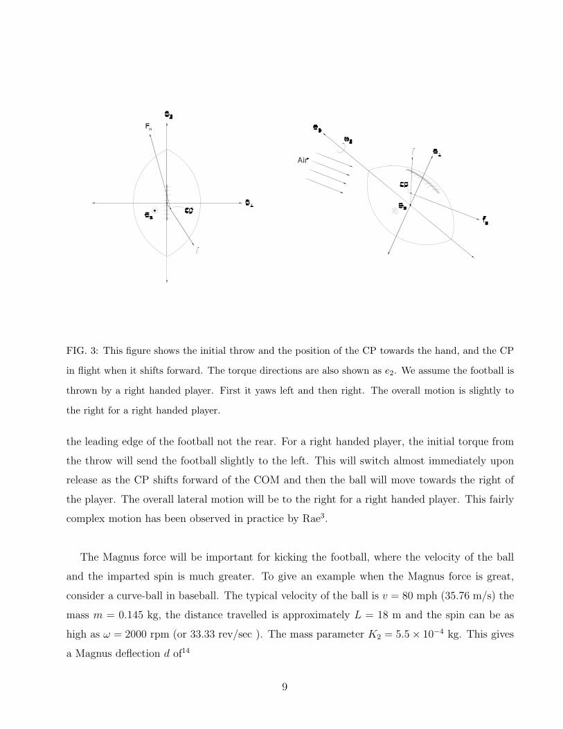
FIG. 3: This figure shows the initial throw and the position of the CP towards the hand, and the CP

in flight when it shifts forward. The torque directions are also shown as e2. We assume the football is

thrown by a right handed player. First it yaws left and then right. The overall motion is slightly to

the right for a right handed player.

the leading edge of the football not the rear. For a right handed player, the initial torque from

the throw will send the football slightly to the left. This will switch almost immediately upon

release as the CP shifts forward of the COM and then the ball will move towards the right of

the player. The overall lateral motion will be to the right for a right handed player. This fairly

complex motion has been observed in practice by Rae3.

The Magnus force will be important for kicking the football, where the velocity of the ball

and the imparted spin is much greater. To give an example when the Magnus force is great,

consider a curve-ball in baseball. The typical velocity of the ball is v = 80 mph (35.76 m/s) the

mass m = 0.145 kg, the distance travelled is approximately L = 18 m and the spin can be as

high as ω = 2000 rpm (or 33.33 rev/sec ). The mass parameter K2 = 5.5 × 10−4 kg. This gives

a Magnus deflection d of14

9

d =K2L

2ω

2mv. (2)

For the curve-ball, d = 0.57 m. Now let us consider typical values for a football. Consider a

pass of length L = 50 m. The football mass is m = 0.411 kg, a throwing velocity of v = 20 m/s

and a spin of ω = 600 rpm ( equivalent to 10 rev/sec). These numbers give a Magnus deflection

of d = 0.8 m for a 50 m pass. This would be hardly noticeable. A strong gust of wind is more

likely to blow the football off course than it is to cause a Magnus force on it. The only way to

really account for a right handed player throwing slightly to the right and a left handed player

throwing slightly to the left would be in the initial throw. This must have to do with finger

positioning, and laces, on one side of the ball or the other.

III. THE THEORY OF FLIGHT

After an extensive search of the literature, we have discovered a detailed analysis on the rigid

dynamics of a football by Brancazio2,4,5. Clear observations of lateral motion, of the type

discussed above, have been made by Rae? . The moments of inertia used are that for an

ellipsoidal shell which have been calculated by subtracting a larger solid ellipsoid of semi–major

and minor axes a + t and b + t from a smaller one with axes a and b. The results are kept in

the first order of the thickness of the shell, t. We have calculated the exact prolate spheroid

shell moments (in Appendix A) and we have also used a parabola of revolution, (calculation in

Appendix B) which we believe more closely fits the shape of a football. Our results are seen to

complement those of Brancazio5.

The angular momentum of a football can only change if there is an applied torque. Aerodynamic

drag on a football can produce the torque required to pitch the ball to align the e3 axis along

the parabolic trajectory2. The air pressure over the leading surface of the football results in a

drag force which acts through the center of pressure (CP). The CP depends on the speed of

the football and the inclination of the e3 axis to the horizontal. For inclinations of zero and 90

degrees there is no torque since the CP is coincident with the COM, ignoring any effect of the

laces. During flight when there is an acute angle of inclination of the e3 axis to the horizontal,

the CP should be slightly forward of the COM, since the air hits the leading edge of the ball. The

10

gyroscopic precession of the ball is caused by this aerodynamic torque. The resulting motion of

the football is very similar to a gyroscope2,6,7 but has extra complexity due to the drag forces

changing with pitch angle of the football. For stability we require that2,

ω3 =

√4τI1

I3

, (3)

where τ = fdℓ sin θ is aerodynamic torque, θ is the angle between the aerodynamic drag force

and the e3 axis, I1and I3 are the moments of inertia in the transverse and long e3 axis directions

and ω3 is the angular velocity of the football about the e3 axis. The gyroscopic precession rate,

defined as the angular rotation rate of the velocity axis about the e3 axis, φ is given by5

φ =fdℓ

I3ω3

(4)

where fd is the aerodynamic drag (which is the cause of torque τ above) and ℓ is the distance

from the CP to the COM. Both of these values will change with the pitch of the ball, hence the

football dynamics is rather more complex than that of a simple top.

For low speeds of the ball, when the aerodynamic drag is small, there can still be a precession

of the football due to an imperfect throw. That is, if there is more than one spin axis of the

football it will precess in flight with no torque. The ball gets most of its spin along the long e3

axis. However, because the ball is held at one end, a small spin is imparted about the transverse

axis. A slight upward tilt of the ball on release is almost unavoidable because the fingers are

pulling down on rear of the ball to produce the spin. Thus, there is an initial moment about

the e1 axis which will tend to pitch the football. This non–zero spin will result in torque–free

precession or wobble.

The aerodynamic drag forces are linearly dependent on the surface area A of the football. The

surface area A would be in the direction of motion. Figure 4(a) shows a football which is

perfectly horizontal, or with zero inclination angle. The vertical surface area 1, it presents has

a maximum area πab and the horizontal surface area 2 it presents has a minimum area πb2.

Figure 4(b) shows a football at angle of inclination α. The surface area has now changed. The

vertical surface area 1 has become πb(a cos α + b sin α) and the horizontal surface has an area

πb(a sin α + b cosα). The velocity of the football can easily be transformed into the vertical and

horizontal components and thus the aerodynamic drag fd can also be written in terms of vertical

and horizontal components for each angle α. The equations of motion are tedious to write out

11

FIG. 4: The surface area the football presents, at different inclination angles in flight. Fig 4(a) show

maximum surface area πab vertically and minimum surface area πb2 horizontally. Fig. 4(b) has an

inclination of α and the surface area this football presents to the vertical and horizontal has changed.

but a computer code can easily be constructed to plot the football position and orientation in

flight. It is recommended that the parabola of rotation moments of inertia be used as the most

accurately fitting the football.

IV. CONCLUSIONS

It appears that footballs, have something in common with natural phenomenon, in that they

tend to follow the path of least resistance (air resistance) and the motion tends to minimize

energy. Also, when in doubt about projectile motion, ask a rocket scientist!

The experimental values of the moments for the football, as determined by Brody15 using a tor-

12

sion pendulum and measuring periods of oscillation are; I1 = 0.00321kg m2 and I3 = 0.00194kg

m2 and the ratio I3/I1 = 0.604. Drag forces on a football have been measured in a wind tunnel

by Watts and Moore11 and independently by Rae and Streit16.

For the prolate spheroid shell football we obtained the following moments of inertia, (these

results were checked numerically on Mathematica 5.2), using a = 0.141 m (or 5.5 in), b = 0.086

m ( or 3.4 in) and M = 0.411 kg were I1 = 0.003428 kgm2 and I3 = 0.002138 kgm2. When

we use the same parameters in our exact formulae (see Appendix A) we find exactly the same

numbers, so we are confident that the above results are correct.

For the parabola of revolution, we get I1 = 0.002829 kgm2 and I3 = 0.001982 kgm2 (see

Appendix B for details). We suggest that the moment of inertia I1 is slightly lower than the

experimental value because of extra leather at the ends due to the seams which we have not

taken into account. This is caused by the four leather panels being sewn together and there

being a little excess material at the ends making the football slightly heavier at the ends than

we have accounted for. If we add a small mass to either end of the football this would account

for the very small increase in the experimentally found value. The increase in moment of inertia

required (experimental value - our value)is ∆I1 = 0.000381 kgm2 which could be accounted

for by a small mass of leather m0/2 at either end of the ball, where ∆I = m0a2 and a is the

semi-major axes 0.141 m. Hence, m0 = 19.164 g (grams) which implies m0/2 = 9.582 grams

excess leather at each end of the ball. This is a very small amount of leather! We believe this

is a more accurate description of the football than the prolate spheroid shell or the solid ellipsoid.

Furthermore, the solid ellipsoid gives quite different moments. For the solid,

I1 = (1/5)m(a2+b2) = 0.002242 kgm2 , for the same a, b as above and I3 = (2/5)mb2 = 0.001216

kgm2.

V. ACKNOWLEDGMENTS

We would like to thank Dr. M. Khakoo of CSU Fullerton for telling us about the “football”

challenge set by Dr. Timothy Gay, at the 37th meeting of the Division of Atomic, Molecular

13

and Optical Physics (DAMOP) meeting in Knoxville Tennessee, May 16–20th 2006. Mr. Horn

completed this project as part of the requirements of a Masters degree in Physics at CSU

Fullerton under the supervision of Prof. H. Fearn.

VI. APPENDIX A

Derivation of the principal moments of inertia of a prolate spheroidal shell (hollow structure).

The football is roughly the shape of a prolate spheroid, which is an ellipsoid with two semi major

axes the same length. The equation for the prolate spheroid is;

x2

b2+

y2

b2+

z2

a2= 1 (5)

where a is the semi major axis aligned along the length of the football. This will be the spin

axis. b is the semi minor axis in both the x and y directions. We assume a > b. In fact for an

official size football we will take a = 5.5 inches and b = 3.4 inches, this will be useful for later

numerical examples. It is appropriate to introduce prolate spheroidal coordinates17, to calculate

the moments of inertia.

x = α sinh ε sin θ cos φ

y = α sinh ε sin θ sin φ

z = α cosh ε cos θ (6)

It is appropriate to introduce the semi major and minor axes by the substitution,

a = α cosh ε

b = α sinh ε (7)

This will then reproduce Eq. 5 above. Hence we use,

x = b sin θ cos φ

y = b sin θ sin φ

z = a cos θ (8)

We also require the surface area of the ellipsoid. This can be calculated once we have the

area element dA equivalent to r2dΩ in spherical polar coordinates. In the prolate spheroidal

14

coordinate system we find,

dA = hθ hφ dθ dφ = (a2 sin2 θ + b2 cos2 θ)1/2b sin θ dθ dφ . (9)

where the usual hk terms are defined by the length element squared,

ds2 = h2ε dε2 + h2

θ dθ2 + h2φ dφ2 . (10)

Now we can easily integrate the area element over all angles, 0 ≤ θ ≤ π and 0 ≤ φ < 2π. We

will need this surface area for the moments of inertia later on. The surface area of the ellipsoid

is;

Area =∫ 2π

0dφ∫ π

0(a2 sin2 θ + b2 cos2 θ)1/2b sin θ dθ

= 2πab∫ 1

−1(1 − e2x2)1/2dx

= 4πab∫ e

0(1 − z2)1/2dz

=4πab

e

∫ sin−1 e

0cos2 θ dθ

⇒ Area = 2πb

(

a sin−1 e

e+ b

)

(11)

where in the first step we set x = cos θ, then z = ex, and then z = sin θ. We used the double

angle formula for sin 2θ = 2 sin θ cos θ and from tables18 we have that sin−1 x = cos−1√

1 − x2

so that cos(sin−1 e) = b/a where e =√

1 − b2/a2. At this point the derivation of the principal

moments of inertia is reasonably straight forward, although a little messy. We introduce the

surface mass density ρ = M/Area, where the Area is that given by Eq. 11, and define the

following principal moments;

I1 = I2 = ρ∫ ∫

(x2 + z2)dA

I3 = ρ∫ ∫

(x2 + y2)dA (12)

where I1 = Ixx , I2 = Iyy and I3 = Izz and dA = (a2 sin2 θ + b2 cos2 θ)1/2b sin θ dθ dφ. To save

space here we give only one derivation, the other being very similar.

I3 = ρ∫ ∫

(x2 + y2)dA

= ρ∫ 2π

0dφ∫ π

0b3 sin3 θ(a2 sin2 θ + b2 cos2 θ)1/2 dθ

15

= 4πab3ρ∫ π/2

0sin3 θ(1 − e2 cos2 θ)1/2 dθ

= 4πab3ρ∫ 1

0(1 − x2)(1 − e2x2)1/2dx

= 4πab3ρ∫ e

0

(

1 −z2

e2

)

(

1 − z2)1/2 dz

e

=4πab3ρ

e

∫ sin−1 e

0

(

cos2 θ −sin2 2θ

4e2

)

dθ

=4πab3ρ

e

[

1

2sin−1 e +

e

2

b

a−

1

8e2sin−1 e +

1

8e

b

a

(

b2

a2− e2

)]

(13)

After substituting for ρ and some algebra we find;

I3 = mb2

(

1 −1

4e2

)

+b2

a2b

2e2(

a sin−1 ee

+ b)

(14)

It should be noted that,(

1 −1

4e2

)

=1

4

(

3a2 − 4b2

a2 − b2

)

ρ =M

2πb(

a sin−1 ee

+ b) . (15)

As an interesting aside, one could also calculate the I3 moment using rings and then integrating

from −a ≤ z ≤ a. This is possible because one can set x2 + y2 = r2 and then from the equation

of a prolate ellipsoid, Eq.(5), arrive at an equation for r(z), r′ and the width of a ring ds as;

r(z) = b

(

1 −z2

a2

)1/2

r′(z) =dr

dz=

bz/a2

(

1 − z2

a2

)1/2

ds =√

dr2 + dz2 =

1 +

(

dr

dz

)2

1/2

dz . (16)

Therefore, with the mass of the ring as dmring = ρ 2πr ds we have;

I3 =∫

r2dmring

= 2πρ∫

r3ds

= 4πρ∫ a

0r3

1 +

(

dr

dz

)2

1/2

dz

= 4πρ∫ a

0b3

(

1 −z2

a2

)(

1 + z2 (b2 − a2)

a4

)1/2

dz (17)

16

which after setting z = a cos θ we arrive at the third line of Eq. (13).

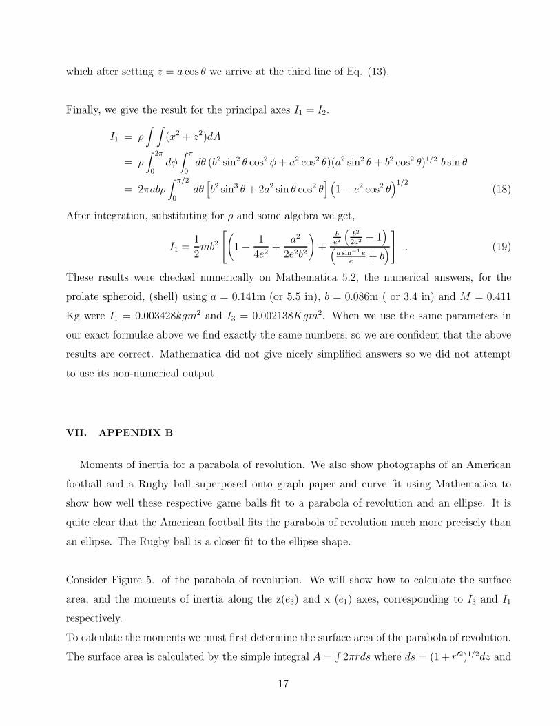
Finally, we give the result for the principal axes I1 = I2.

I1 = ρ∫ ∫

(x2 + z2)dA

= ρ∫ 2π

0dφ∫ π

0dθ (b2 sin2 θ cos2 φ + a2 cos2 θ)(a2 sin2 θ + b2 cos2 θ)1/2 b sin θ

= 2πabρ∫ π/2

0dθ[

b2 sin3 θ + 2a2 sin θ cos2 θ] (

1 − e2 cos2 θ)1/2

(18)

After integration, substituting for ρ and some algebra we get,

I1 =1

2mb2

(

1 −1

4e2+

a2

2e2b2

)

+

be2

(

b2

2a2 − 1)

(

a sin−1 ee

+ b)

. (19)

These results were checked numerically on Mathematica 5.2, the numerical answers, for the

prolate spheroid, (shell) using a = 0.141m (or 5.5 in), b = 0.086m ( or 3.4 in) and M = 0.411

Kg were I1 = 0.003428kgm2 and I3 = 0.002138Kgm2. When we use the same parameters in

our exact formulae above we find exactly the same numbers, so we are confident that the above

results are correct. Mathematica did not give nicely simplified answers so we did not attempt

to use its non-numerical output.

VII. APPENDIX B

Moments of inertia for a parabola of revolution. We also show photographs of an American

football and a Rugby ball superposed onto graph paper and curve fit using Mathematica to

show how well these respective game balls fit to a parabola of revolution and an ellipse. It is

quite clear that the American football fits the parabola of revolution much more precisely than

an ellipse. The Rugby ball is a closer fit to the ellipse shape.

Consider Figure 5. of the parabola of revolution. We will show how to calculate the surface

area, and the moments of inertia along the z(e3) and x (e1) axes, corresponding to I3 and I1

respectively.

To calculate the moments we must first determine the surface area of the parabola of revolution.

The surface area is calculated by the simple integral A =∫

2πrds where ds = (1 + r′2)1/2dz and

17

FIG. 5: Parabola of revolution, with equation r(z) = b− z2/(4a), the length of the football is 2x where

x = 2√

ab

r′ = dr/dz. We define the semi–major axis here to be x = 2√

ab which will simplify the

integrations considerably. Using the parabolic equation r(z) = b − z2/(4a) we find that the

surface area of revolution is given by,

A =∫

2πr(z)ds

= 2π∫ x

−xr[1 + r′2]1/2 dz

= 2πb2

∫ x

−x

(

1 −z2

x2

)(

1

b2+

4z2

x4

)1/2

dz (20)

(21)

This can easily be solved on mathematica and the result for x = 0.141 m and b = 0.086 m is

found to be A = 0.114938 m2. The calculation can be done by hand but it is very long winded

and tedious. We have not written out the full expression because it does not lead to any great

insight.

The moment of inertia for the e3, or long axis, is found most easily by summing over rings.

Using the area of a ring to be 2πrds and the mass of a ring is dmring = ρ2πrds where ρ = M/A,

M = 0.411kg, is the total mass of the football and A is the surface area given above.

18

I3 =∫

r2dm

= 2πρ∫

r3ds

= 2πρb4

∫ x

−x

(

1 −z2

x2

)3 (

1

b2+

4z2

x4

)1/2

dz (22)

(23)

Making substitutions of the form z = ix2 sin θ/(2b) simplifies the square root term and may

allow you to solve this and the I1 below by hand, but we would not recommend it. Mathematica

again comes to the rescue and we find a value of I3 = 0.001982 kgm2.

There are two ways to proceed with the moment of inertia about the e1 or x axis. You can chop

the football into rings again and use the parallel axis theorem. Or you can directly integrate

over the surface using small elemental areas. We show the small area method below. Consider

a small area of the surface and take the mass to be dm = ρdA. Then the contribution of this

small area to the moment about e1 is given by dI1 = ρ(y2 + z2)dA. We have taken the vertical

(or e2) axis to be y here. Convert to polar coordinates, using x = r cos θ and y = r sin θ. Note

that x2 + y2 = r2 since there is a circular cross–section. In the xy direction we may change to

polar coordinates, rdθ. In the z-direction we must use the length ds for accuracy. Therefore, an

element of the surface has an area dA = rdθ ds where ds is defined above.

I1 = 2ρ∫ 2π

0dθ

∫ x

0ds r(y2 + z2)

= 2ρ∫ x

0

∫ 2π

0

(

1 −z2

x2

)(

1 +4b2z2

x4

)1/2

b2

(

1 −z2

x2

)2

sin2 θ + z2

dθ dz

= 2πρ∫ x

0

(

1 −z2

x2

)(

1 +4b2z2

x4

)1/2

b2

(

1 −z2

x2

)2

+ 2z2

dz

(24)

For the parabola of revolution, we get I1 = 0.002829 kg m2.

To clarify our point, we show photographs of both an American football (pro NFL game ball)

above and a Rugby ball below. The photographs were taken with both balls on top of graph

19

FIG. 6: American Football Photo and curve fit. Plot(a) shows the photograph of the football with the

outline of the curve fitting to show how well they match. Plot(b) shows the curve fit from Mathematica

alone with the points taken from the original photograph of the football.

paper. We used the outer edge of each photograph of the ball to get points to plot and curve

fit with Mathematica 5.2. The results are shown in figures 6 and 7.

From figures 6 and 7 we see that the American football closely fits the shape of a parabola of

revolution. The rugby ball more closely fits the shape of an ellipsoid.

20

FIG. 7: Rugby ball Photo and curve fit. Plot(a) shows the photograph of the rugby ball with the outline

of the curve fitting to show how well they match. Plot(b) shows the curve fit from Mathematica alone

with the points taken from the original photograph of the rugby ball.

1 Timothy J. Gay, Football Physics: The science of the game Holtzbrinck Publishers (2004).

2 P. J. Brancazio, “Why does a football keep its axis pointing along its trajectory?”, The Physics

teacher, 23, 4571–573 (1985).

3 W. J. Rae, “‘Flight dynamics of an American football in a forward pass”, Sports Engineering, 6,

149–164 (2003).

4 P. J. Brancazio, “The physics of kicking a football”, The Physics teacher, 23, 403–407 (1985).

5 P. J. Brancazio, “Rigid Body Dynamics of a football”, Am. J. Phys., 55, 415–420 (1987).

6 Herbert Goldstein, Charles Poole and John Safko, Classical mechanics, 3rd ed., Addison Wesley,

New York (2002).

7 Jerry B. Marion and Steven T. Thornton, Classical Dynamics of Particles and systems, 4th ed.,

Harcourt College Publishers, New York (1995).

21

8 Chris J. Nowak et al., “Flight Data Recorder for an American Football”,

http://mechatronics.eng.buffalo.edu/research/Football/football recorder.pdf

9 Craig C. Freudenrich, “How the physics of football works”,

http://entertainment.howstuffworks.com/physics-of-football.htm

10 http://rjccourt85.tripod.com/field.html, http://www.wilson.com.

11 Robert G. Watts and Gary Moore, “ The Drag Force on an American football”, Am. J. Phys., 71,

(8), 791–793 (2003).

12 A Physicists Desk Reference, 2nd ed., IOP Press, Springer (1989).

13 W. T. Thomson, Introduction to Space dynamics, Dover Publications Inc., New York (1986).

14 R. G. Watts and R. Ferrer, “The lateral force on a spinning sphere: Aerodynamics of a curveball”,

Am. J. Phys. 55, 40–44 (1987).

15 H. Brody, The Physics Teacher 23, 403 (1985).

16 W. J. Rae and R. J. Streit, “Wind tunnel measurements of the aerodynamic loads on an American

football”, Sports Engineering 5, 165–172 (2002)

17 Murray R. Spiegel, Vector Analysis and an introduction to tensor analysis, Schaum’s outline series,

McGraw Hill book company, New York (1974).

18 I. S. Gradshteyn and I. M. Ryzhim, Tables of Integrals, Series and Products, Academic Press, New

York, 5th ed. (1994). See p56 section 1.624.

22