Physics 42200

Waves & Oscillations

Spring 2013 SemesterMatthew Jones

Lecture 22 – Review

Midterm Exam:

Date: Wednesday, March 6th

Time: 8:00 – 10:00 pm

Room: PHYS 203

Material: French, chapters 1-8

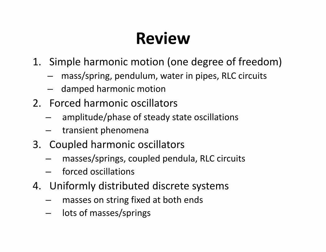
Review

1. Simple harmonic motion (one degree of freedom)

– mass/spring, pendulum, water in pipes, RLC circuits

– damped harmonic motion

2. Forced harmonic oscillators

– amplitude/phase of steady state oscillations

– transient phenomena

3. Coupled harmonic oscillators

– masses/springs, coupled pendula, RLC circuits

– forced oscillations

4. Uniformly distributed discrete systems

– masses on string fixed at both ends

– lots of masses/springs

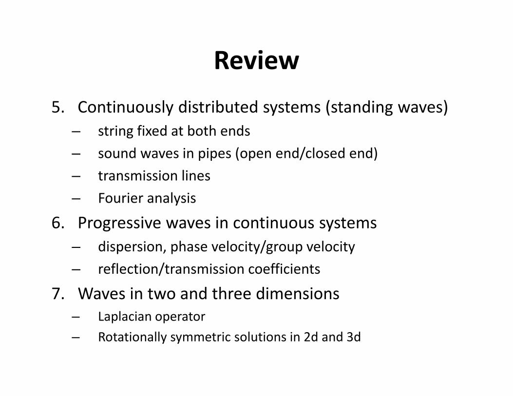
Review

5. Continuously distributed systems (standing waves)

– string fixed at both ends

– sound waves in pipes (open end/closed end)

– transmission lines

– Fourier analysis

6. Progressive waves in continuous systems

– dispersion, phase velocity/group velocity

– reflection/transmission coefficients

7. Waves in two and three dimensions

– Laplacian operator

– Rotationally symmetric solutions in 2d and 3d

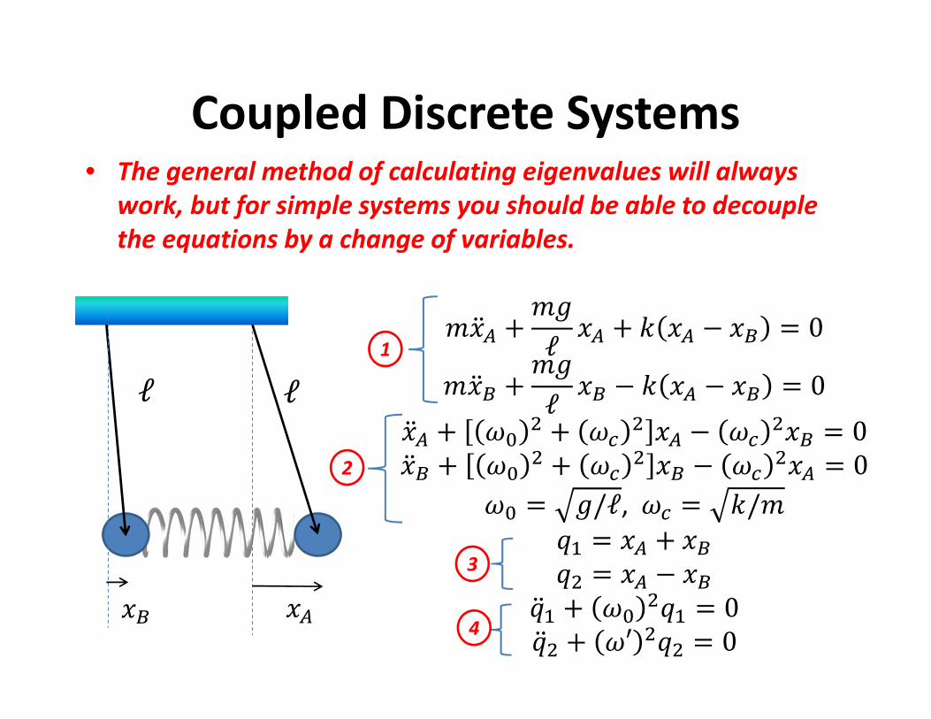
Coupled Discrete Systems• The general method of calculating eigenvalues will always

work, but for simple systems you should be able to decouple

the equations by a change of variables.

ℓ

�� ��

ℓ���� + ��

ℓ �� + �� − �� = 0���� + ��

ℓ �� − �� − �� = 0��� + � � + � � �� − � ��� = 0��� + � � + � � �� − � ��� = 0

� = �/ℓ, � = /��� = �� + ���� = �� − ����� + � ��� = 0

��� + ′ ��� = 0

1

4

3

2

Forced Oscillations

• We mainly considered the qualitative aspects

– We did not analyze the behavior when damping forces

were significant

• Main features:

– Resonance occurs at each normal mode frequency

– Phase difference is � = � 2⁄ at resonance

• Example: �� driven by the force � = �� ��� �– Calculate force term applied to normal coordinates

�� = �� = �� cos �– Reduced to two one-dimensional forced oscillators:

��� + � ��� = ��/� cos ���� + ′ ��� = ��/� cos �

Equations of motion for masses in the middle:

��! + 2 � ��! − � � �!"� + �!#� = 0 � � = �⁄

� � � �

Uniformly Distributed Discrete Systems

ℓ

$�% + 2 � �$% − � � $%#� + $%"� = 0 � � = & �ℓ⁄

• Proposed solution:

�% � = '% cos �'%"� + '%#�

'%= − � + 2 � �

� �• We solved this to determine '% and (:

'%,( = * sin -�. + 1

( = 2 � sin �2 . + 1

• General solution:

�% � = 01( sin -�. + 1

2

(3�cos (� − �(

Uniformly Distributed Discrete Masses

• Amplitude of mass - for normal mode :

'%,( = * sin -�. + 1

• Frequency of normal mode :

( = 2 � sin �2 . + 1

• Solution for normal modes:

�% � = '%,( cos (�• General solution:

�% � = 01( sin -�. + 1

2

(3�cos (� − �(

Vibrations of Continuous Systems

Masses on a String

First normal mode

Second normal mode

Lumped LC Circuit

−4 56%5� − 1

* 7 6% − 6%#� 5� − 1* 7 6% − 6%"� 5� = 0

5�6%5�� + 2 ��6% − ��(6%"� + 6%#�) = 0

;<

;<

;<

;6%(�) 6%#�(�)6%"�(�)

This is the exact same problem as the previous two examples.

Forced Coupled Oscillators

• Qualitative features are the same:

– Motion can be decoupled into a set of .independent oscillator equations (normal modes)

– Amplitude of normal mode oscillations are large

when driven with the frequency of the normal

mode

– Phase difference approaches �/2 at resonance

• You should be able to anticipate the

qualitative behavior when coupled oscillators

are driven by a periodic force.

Continuous Distributions

Limit as . → ∞ and � ℓ⁄ → ?:

@�$@�� = 1

A�@�$@��

Boundary conditions specified at � = 0 and � = 4:

– Fixed ends: $ 0 = $ 4 = 0– Maximal motion at ends: $B 0 = $B 4 = 0– Mixed boundary conditions

Normal modes will be of the form

$% �, � = '% sin(%�) cos( %� − �%)or $% �, � = '% cos(%�) cos( %� − �%)

Properties of the Solutions

$ 4, � ~ sin %4 = 0 ⇒ %4 = -�

E% = 24-

% = -�A4

F% = -A24

Boundary Conditions

• Examples:

– String fixed at both ends: $ 0 = $ 4 = 0– Organ pipe open at one end: $B 0 = $B 4 = 0

• Driving end has maximal pressure amplitude

– Organ pipe closed at one end: $B 0 = 0, $ 4 = 0– Transmission line open at one end: 6 4 = 0– Transmission line shorted at one end: A 4 ∝ H! I

HJ = 0

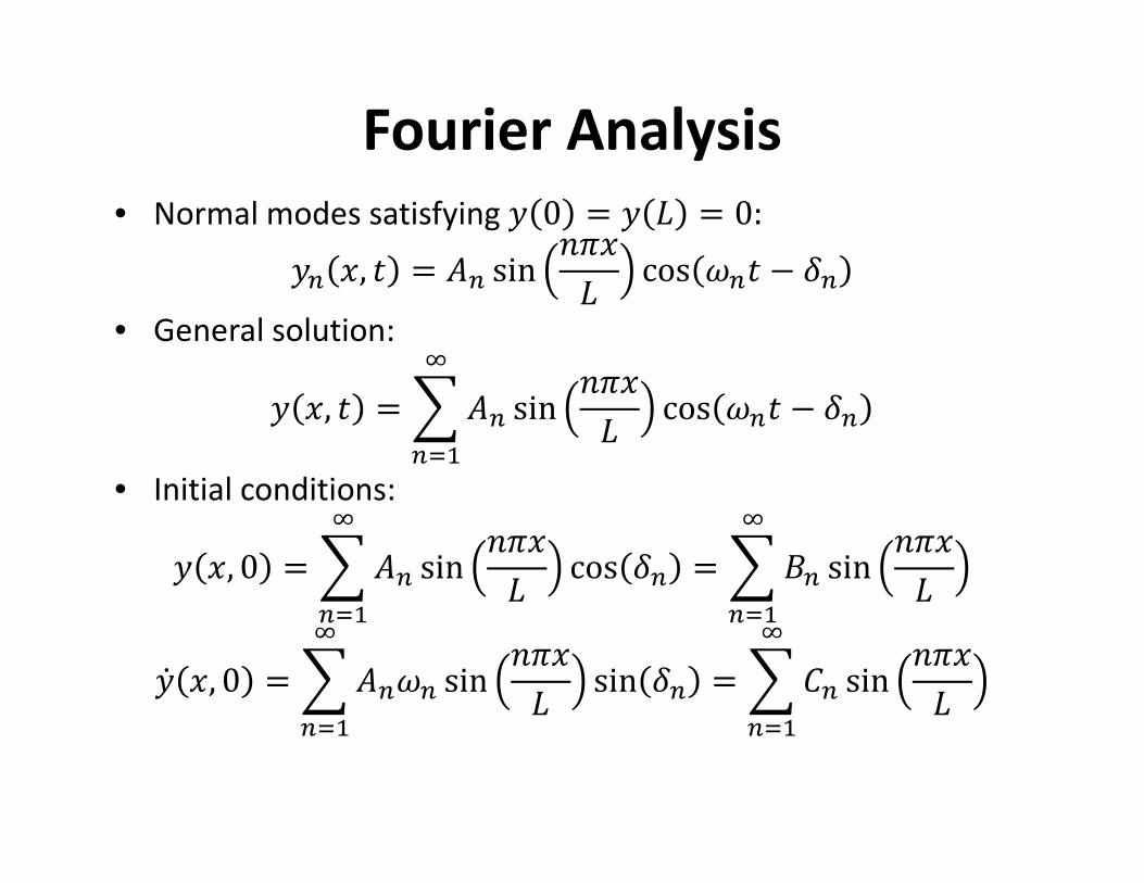
Fourier Analysis

• Normal modes satisfying $ 0 = $ 4 = 0:$% �, � = '% sin -��

4 cos %� − �%• General solution:

$ �, � = 0 '% sin -��4 cos %� − �%

L

%3�• Initial conditions:

$ �, 0 = 0 '% sin -��4 cos �%

L

%3�= 0 M% sin -��

4L

%3�

$B �, 0 = 0 '% % sin -��4 sin �%

L

%3�= 0 *% sin -��

4L

%3�

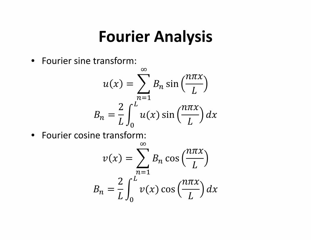
Fourier Analysis

• Fourier sine transform:

N � = 0 M% sin -��4

L

%3�M% = 2

47 N(�) sin -��4 5�

I

�• Fourier cosine transform:

A � = 0 M% cos -��4

L

%3�M% = 2

47 A(�) cos -��4 5�

I

�

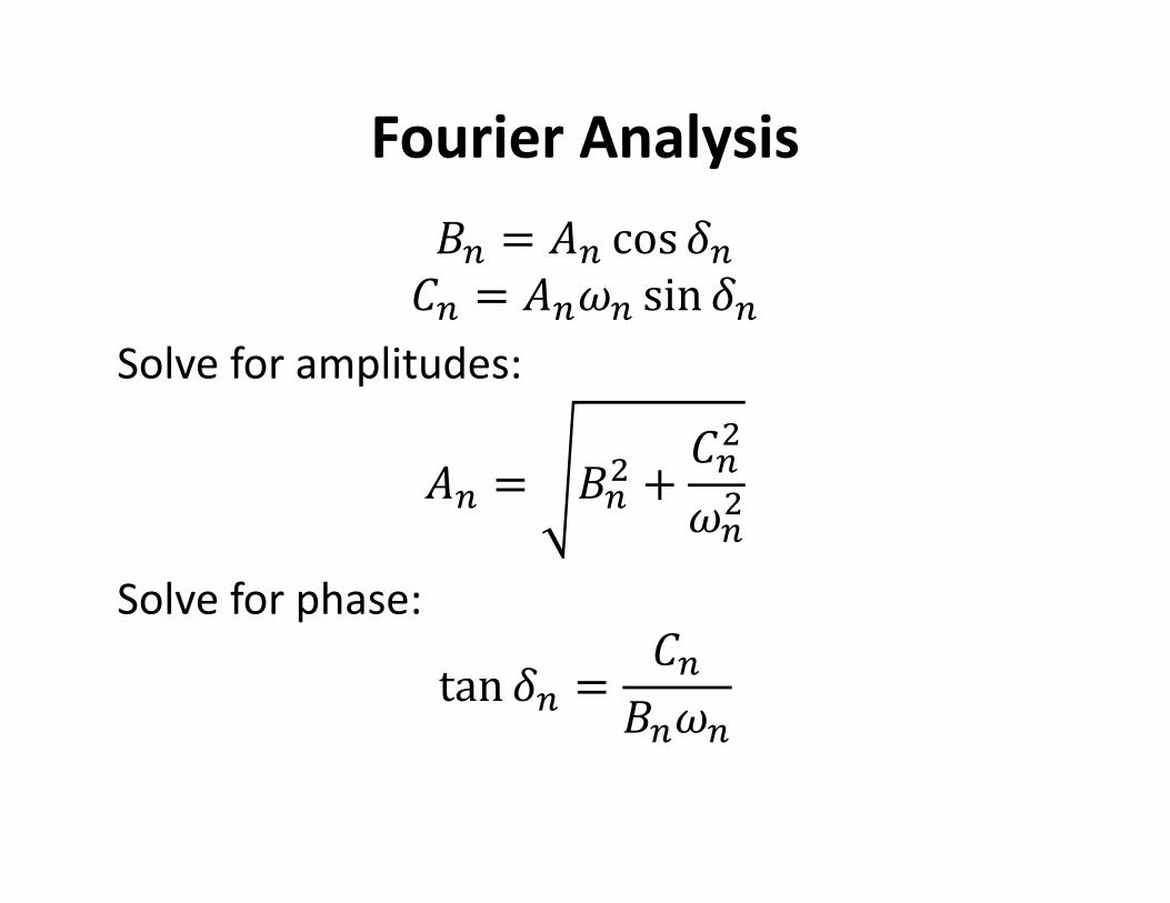
Fourier Analysis

M% = '% cos �%*% = '% % sin �%Solve for amplitudes:

'% = M%� + *%� %�

Solve for phase:

tan �% = *%M% %

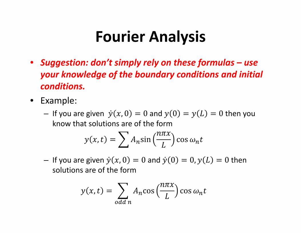
Fourier Analysis

• Suggestion: don’t simply rely on these formulas – use

your knowledge of the boundary conditions and initial

conditions.

• Example:

– If you are given $B �, 0 = 0 and $ 0 = $ 4 = 0 then you

know that solutions are of the form

$ �, � = 0'%sin -��4 cos %�

– If you are given $B �, 0 = 0 and $B 0 = 0, $ 4 = 0 then

solutions are of the form

$ �, � = 0 '%cos -��4 cos %�

QHH%

Progressive Waves

• Far from the boundaries, other descriptions are more

transparent:

$ �, � = F � ± A�• The Fourier transform gives the frequency components:

' = 12�7 �(�) cos � 5�

L

"LM = 1

2�7 �(�) sin � 5�L

"L

�(�) = 12�7 ' cos(�) 5

L

"L+ 1

2�7 M sin(�) 5L

"L• Narrow pulse in space � wide range of frequencies

• Pulse spread out in space � narrow range of frequencies

Properties of Progressive Waves

• Power carried by a wave:

– String with tension & and mass per unit length ?S = 1

2? �'�A = 12T �'�

• Impedance of the medium:

T = ?A = &/A• Important properties:

– Impedance is a property of the medium, not the wave

– Energy and power are proportional to the square of the

amplitude

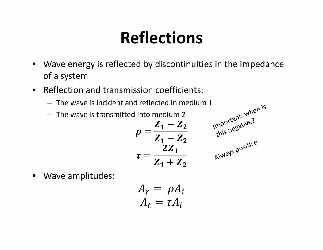
Reflections

• Wave energy is reflected by discontinuities in the impedance

of a system

• Reflection and transmission coefficients:

– The wave is incident and reflected in medium 1

– The wave is transmitted into medium 2

U = VW − VXVW + VX

Y = XVWVW + VX

• Wave amplitudes:

'Z = ['!'J = \'!

Reflected and Transmitted Power

• Power is proportional to the square of the

amplitude.

– Reflected power: SZ = [�S!– Transmitted power: SJ = \�S!

• You should be able to demonstrate that energy is

conserved:

ie, show that ]^ = ]_ + ]`

Dispersion

• Wave speed is sometimes a function of frequency.

• Phase velocity: A = EF = a( (constant)

• Group velocity: Ab = HaH( (function of frequency)

• Energy that is carried by a pulse propagates with the

group velocity

• In optics, A = �/-() and

Ab = A 1 − -5-5

(evaluated at the average wavenumber of the pulse)

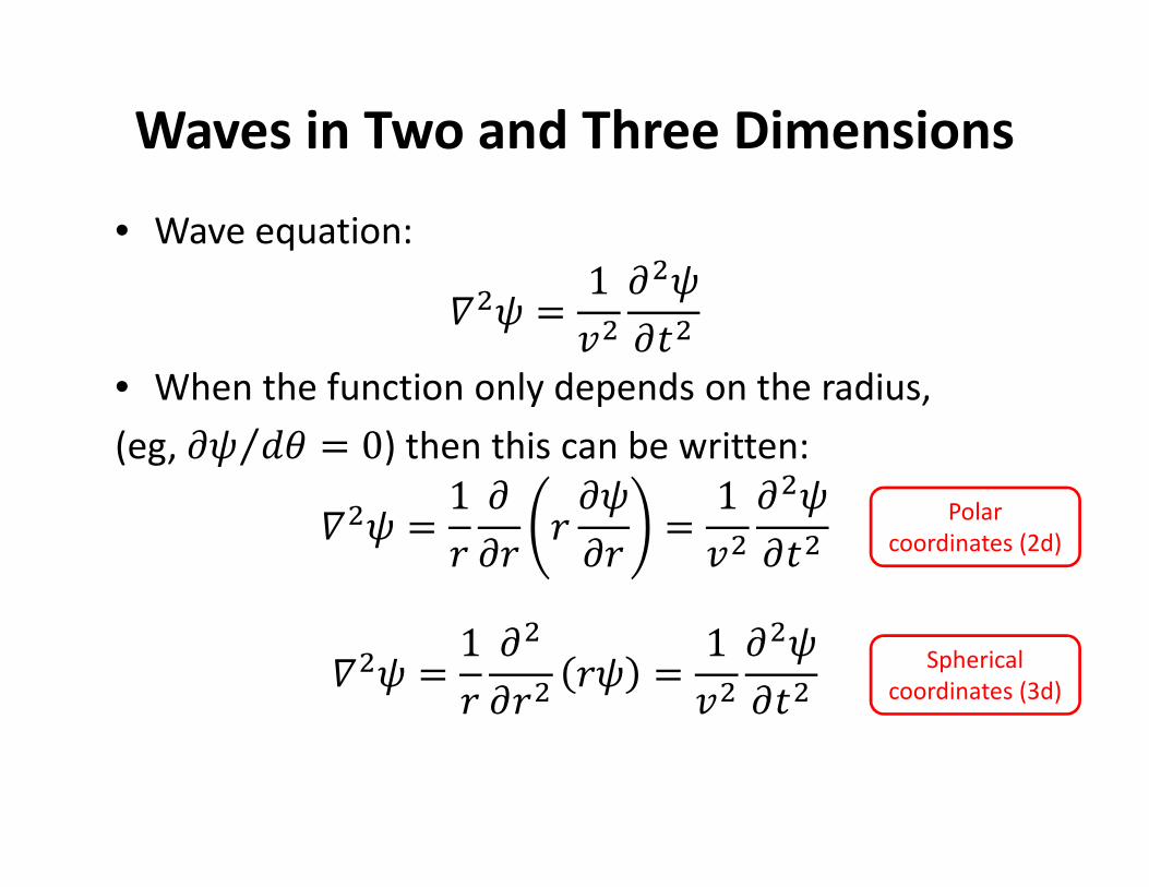
Waves in Two and Three Dimensions

• Wave equation:

c�d = 1A�

@�d@��

• When the function only depends on the radius,

(eg, @d 5e⁄ = 0) then this can be written:

c�d = 1f

@@f f @d

@f = 1A�

@�d@��

c�d = 1f

@�@f� fd = 1

A�@�d@��

Polar

coordinates (2d)

Spherical

coordinates (3d)

Waves in Two Dimensions

• Wave equation in polar coordinates:

c�d = 1f

@@f f @d

@f = 1A�

@�d@��

• Bessel’s equation:

@�d@f� + 1

f@d@f + �

A� d = 0@�d@g� + 1

g@d@g + d(g) = 0

• Solutions: h�(g)~ �i

jkl m"i/nm and o�(g)~ �

ilpq m"i/n

m

Let g = fwhere = /A

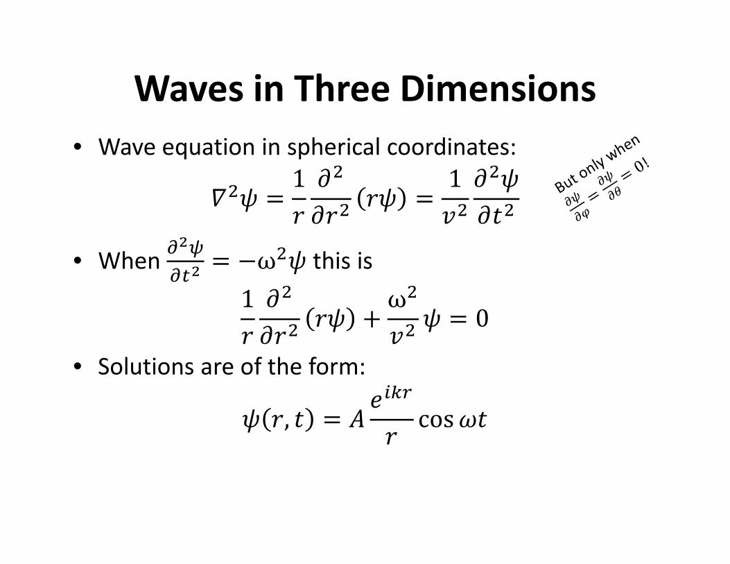
Waves in Three Dimensions

• Wave equation in spherical coordinates:

c�d = 1f

@�@f� fd = 1

A�@�d@��

• When rstrJs = −ω�d this is

1f

@�@f� fd + ω�

A� d = 0• Solutions are of the form:

d f, � = ' v!(Zf cos �

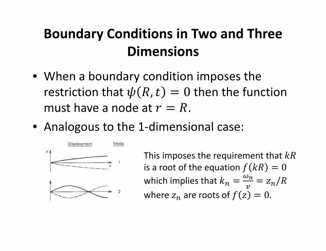
Boundary Conditions in Two and Three

Dimensions

• When a boundary condition imposes the

restriction that d w, � = 0 then the function

must have a node at f = w.

• Analogous to the 1-dimensional case:

This imposes the requirement that wis a root of the equation F w = 0which implies that % = ax

y = g%/wwhere g% are roots of F g = 0.

That’s all for now…

• Study these topics – make sure you

understand the examples and assignment

questions.

• Send e-mail if you would like specific examples

discussed before the exam next Wednesday.

• Next topics: waves applied to optics.