physical review d searches for periodic gravitational

Searches for periodic gravitational waves from unknown isolated sources and Scorpius X-1:Results from the second LIGO science run

B. Abbott,15 R. Abbott,15 R. Adhikari,15 J. Agresti,15 P. Ajith,2 B. Allen,2,54 R. Amin,19 S. B. Anderson,15

W. G. Anderson,54 M. Arain,41 M. Araya,15 H. Armandula,15 M. Ashley,4 S Aston,40 P. Aufmuth,38 C. Aulbert,1 S. Babak,1

S. Ballmer,15 H. Bantilan,9 B. C. Barish,15 C. Barker,16 D. Barker,16 B. Barr,42 P. Barriga,53 M. A. Barton,42 K. Bayer,18

K. Belczynski,26 S. J. Berukoff,1 J. Betzwieser,18 P. T. Beyersdorf,29 B. Bhawal,15 I. A. Bilenko,23 G. Billingsley,15

R. Biswas,54 E. Black,15 K. Blackburn,15 L. Blackburn,18 B. Blair,53 B. Bland,16 J. Bogenstahl,42 L. Bogue,17 R. Bork,15

V. Boschi,15 S. Bose,56 P. R. Brady,54 V. B. Braginsky,23 J. E. Brau,45 M. Brinkmann,2 A. Brooks,39 D. A. Brown,15,7

A. Bullington,32 A. Bunkowski,2 A. Buonanno,43 O. Burmeister,2 D. Busby,15 W. E. Butler,46 R. L. Byer,32 L. Cadonati,18

G. Cagnoli,42 J. B. Camp,24 J. Cannizzo,24 K. Cannon,54 C. A. Cantley,42 J. Cao,18 L. Cardenas,15 K. Carter,17

M. M. Casey,42 G. Castaldi,48 C. Cepeda,15 E. Chalkey,42 P. Charlton,10 S. Chatterji,15 S. Chelkowski,2 Y. Chen,1

F. Chiadini,47 D. Chin,44 E. Chin,53 J. Chow,4 N. Christensen,9 J. Clark,42 .P Cochrane,2 T. Cokelaer,8 C. N. Colacino,40

R. Coldwell,41 M. Coles,17 R. Conte,47 D. Cook,16 T. Corbitt,18 D. Coward,53 D. Coyne,15 J. D. E. Creighton,54

T. D. Creighton,15 R. P. Croce,48 D. R. M. Crooks,42 A. M. Cruise,40 P. Csatorday,18 A. Cumming,42 C. Cutler,7

J. Dalrymple,33 E. D’Ambrosio,15 K. Danzmann,38,2 G. Davies,8 E. Daw,49 D. DeBra,32 J. Degallaix,53 M. Degree,32

T. Delker,41 T. Demma,48 V. Dergachev,44 S. Desai,34 R. DeSalvo,15 S. Dhurandhar,14 M. Dıaz,35 J. Dickson,4

A. Di Credico,33 G. Diederichs,38 A. Dietz,8 H. Ding,15 E. E. Doomes,31 R. W. P. Drever,5 J.-C. Dumas,53 R. J. Dupuis,15

J. G. Dwyer,11 P. Ehrens,15 E. Espinoza,15 T. Etzel,15 M. Evans,15 T. Evans,17 S. Fairhurst,8,15 Y. Fan,53 D. Fazi,15

M. M. Fejer,32 L. S. Finn,34 V. Fiumara,47 N. Fotopoulos,54 A. Franzen,38 K. Y. Franzen,41 A. Freise,40 R. Frey,45

T. Fricke,46 P. Fritschel,18 V. V. Frolov,17 M. Fyffe,17 V. Galdi,48 K. S. Ganezer,6 J. Garofoli,16 I. Gholami,1

J. A. Giaime,17,19 S. Giampanis,46 K. D. Giardina,17 K. Goda,18 E. Goetz,44 L. M. Goggin,15 G. Gonzalez,19 S. Gossler,4

A. Grant,42 S. Gras,53 C. Gray,16 M. Gray,4 J. Greenhalgh,28 A. M. Gretarsson,12 R. Grosso,35 H. Grote,2 S. Grunewald,1

M. Guenther,16 R. Gustafson,44 B. Hage,38 D. Hammer,54 C. Hanna,19 J. Hanson,17 J. Harms,2 G. Harry,18 E. Harstad,45

T. Hayler,28 J. Heefner,15 G. Heinzel,2 I. S. Heng,42 A. Heptonstall,42 M. Heurs,2 M. Hewitson,2 S. Hild,38 E. Hirose,33

D. Hoak,17 D. Hosken,39 J. Hough,42 E. Howell,53 D. Hoyland,40 S. H. Huttner,42 D. Ingram,16 E. Innerhofer,18 M. Ito,45

Y. Itoh,54 A. Ivanov,15 D. Jackrel,32 O. Jennrich,42 B. Johnson,16 W. W. Johnson,19 W. R. Johnston,35 D. I. Jones,50

G. Jones,8 R. Jones,42 L. Ju,53 P. Kalmus,11 V. Kalogera,26 D. Kasprzyk,40 E. Katsavounidis,18 K. Kawabe,16

S. Kawamura,25 F. Kawazoe,25 W. Kells,15 D. G. Keppel,15 F. Ya. Khalili,23 C. J. Killow,42 C. Kim,26 P. King,15

J. S. Kissell,19 S. Klimenko,41 K. Kokeyama,25 V. Kondrashov,15 R. K. Kopparapu,19 D. Kozak,15 B. Krishnan,1 P. Kwee,38

P. K. Lam,4 M. Landry,16 B. Lantz,32 A. Lazzarini,15 B. Lee,53 M. Lei,15 J. Leiner,56 V. Leonhardt,25 I. Leonor,45

K. Libbrecht,15 A. Libson,9 P. Lindquist,15 N. A. Lockerbie,51 J. Logan,15 M. Longo,47 M. Lormand,17 M. Lubinski,16

H. Luck,38,2 B. Machenschalk,1 M. MacInnis,18 M. Mageswaran,15 K. Mailand,15 M. Malec,38 V. Mandic,15 S. Marano,47

S. Marka,11 J. Markowitz,18 E. Maros,15 I. Martin,42 J. N. Marx,15 K. Mason,18 L. Matone,11 V. Matta,47 N. Mavalvala,18

R. McCarthy,16 D. E. McClelland,4 S. C. McGuire,31 M. McHugh,21 K. McKenzie,4 J. W. C. McNabb,34 S. McWilliams,24

T. Meier,38 A. Melissinos,46 G. Mendell,16 R. A. Mercer,41 S. Meshkov,15 E. Messaritaki,15 C. J. Messenger,42 D. Meyers,15

E. Mikhailov,18 S. Mitra,14 V. P. Mitrofanov,23 G. Mitselmakher,41 R. Mittleman,18 O. Miyakawa,15 S. Mohanty,35

G. Moreno,16 K. Mossavi,2 C. MowLowry,4 A. Moylan,4 D. Mudge,39 G. Mueller,41 S. Mukherjee,35 H. Muller-Ebhardt,2

J. Munch,39 P. Murray,42 E. Myers,16 J. Myers,16 S. Nagano,2 T. Nash,15 G. Newton,42 A. Nishizawa,25 F. Nocera,15

K. Numata,24 P. Nutzman,26 B. O’Reilly,17 R. O’Shaughnessy,26 D. J. Ottaway,18 H. Overmier,17 B. J. Owen,34 Y. Pan,43

M. A. Papa,1,54 V. Parameshwaraiah,16 C. Parameswariah,17 P. Patel,15 M. Pedraza,15 S. Penn,13 V. Pierro,48 I. M. Pinto,48

M. Pitkin,42 H. Pletsch,2 M. V. Plissi,42 F. Postiglione,47 R. Prix,1 V. Quetschke,41 F. Raab,16 D. Rabeling,4 H. Radkins,16

R. Rahkola,45 N. Rainer,2 M. Rakhmanov,34 M. Ramsunder,34 K. Rawlins,18 S. Ray-Majumder,54 V. Re,40 T. Regimbau,8

H. Rehbein,2 S. Reid,42 D. H. Reitze,41 L. Ribichini,2 S. Richman,18 R. Riesen,17 K. Riles,44 B. Rivera,16

N. A. Robertson,15,42 C. Robinson,8 E. L. Robison,40 S. Roddy,17 A. Rodriguez,19 A. M. Rogan,56 J. Rollins,11

J. D. Romano,8 J. Romie,17 H. Rong,41 R. Route,32 S. Rowan,42 A. Rudiger,2 L. Ruet,18 P. Russell,15 K. Ryan,16

S. Sakata,25 M. Samidi,15 L. Sancho de la Jordana,37 V. Sandberg,16 G. H. Sanders,15 V. Sannibale,15 S. Saraf,27 P. Sarin,18

B. Sathyaprakash,8 S. Sato,25 P. R. Saulson,33 R. Savage,16 P. Savov,7 A. Sazonov,41 S. Schediwy,53 R. Schilling,2

R. Schnabel,2 R. Schofield,45 B. F. Schutz,1,8 P. Schwinberg,16 S. M. Scott,4 A. C. Searle,4 B. Sears,15 F. Seifert,2

D. Sellers,17 A. S. Sengupta,8 P. Shawhan,43 D. H. Shoemaker,18 A. Sibley,17 J. A. Sidles,52 X. Siemens,15,7 D. Sigg,16

S. Sinha,32 A. M. Sintes,37,1 B. J. J. Slagmolen,4 J. Slutsky,19 J. R. Smith,2 M. R. Smith,15 K. Somiya,2,1 K. A. Strain,42

PHYSICAL REVIEW D 76, 082001 (2007)

1550-7998=2007=76(8)=082001(35) 082001-1 © 2007 The American Physical Society

N. E. Strand,34 D. M. Strom,45 A. Stuver,34 T. Z. Summerscales,3 K.-X. Sun,32 M. Sung,19 P. J. Sutton,15 J. Sylvestre,15

H. Takahashi,1 A. Takamori,15 D. B. Tanner,41 M. Tarallo,15 R. Taylor,15 R. Taylor,42 J. Thacker,17 K. A. Thorne,34

K. S. Thorne,7 A. Thuring,38 M. Tinto,5 K. V. Tokmakov,42 C. Torres,35 C. Torrie,42 G. Traylor,17 M. Trias,37 W. Tyler,15

D. Ugolini,36 C. Ungarelli,40 K. Urbanek,32 H. Vahlbruch,38 M. Vallisneri,7 C. Van Den Broeck,8 M. van Putten,18

M. Varvella,15 S. Vass,15 A. Vecchio,40 J. Veitch,42 P. Veitch,39 A. Villar,15 C. Vorvick,16 S. P. Vyachanin,23

S. J. Waldman,15 L. Wallace,15 H. Ward,42 R. Ward,15 K. Watts,17 D. Webber,15 A. Weidner,2 M. Weinert,2 A. Weinstein,15

R. Weiss,18 L. Wen,1 S. Wen,19 K. Wette,4 J. T. Whelan,1 D.. M. Whitbeck,34 S. E. Whitcomb,15 B. F. Whiting,41 S. Wiley,6

C. Wilkinson,16 P. A. Willems,15 L. Williams,41 B. Willke,38,2 I. Wilmut,28 W. Winkler,2 C. C. Wipf,18 S. Wise,41

A. G. Wiseman,54 G. Woan,42 D. Woods,54 R. Wooley,17 J. Worden,16 W. Wu,41 I. Yakushin,17 H. Yamamoto,15 Z. Yan,53

S. Yoshida,30 N. Yunes,34 K. D. Zaleski,34 M. Zanolin,18 J. Zhang,44 L. Zhang,15 C. Zhao,53 N. Zotov,20 M. Zucker,18

H. zur Muhlen,38 and J. Zweizig15

(LIGO Scientific Collaboration)*

1Albert-Einstein-Institut, Max-Planck-Institut fur Gravitationsphysik, D-14476 Golm, Germany2Albert-Einstein-Institut, Max-Planck-Institut fur Gravitationsphysik, D-30167 Hannover, Germany

3Andrews University, Berrien Springs, Michigan 49104, USA4Australian National University, Canberra, 0200, Australia

5California Institute of Technology, Pasadena, California 91125, USA6California State University, Dominguez Hills, Carson, California 90747, USA

7Caltech-CaRT, Pasadena, California 91125, USA8Cardiff University, Cardiff, CF2 3YB, United Kingdom9Carleton College, Northfield, Minnesota 55057, USA

10Charles Sturt University, Wagga Wagga, NSW 2678, Australia11Columbia University, New York, New York 10027, USA

12Embry-Riddle Aeronautical University, Prescott, AZ 86301 USA13Hobart and William Smith Colleges, Geneva, New York 14456, USA

14Inter-University Centre for Astronomy and Astrophysics, Pune - 411007, India15LIGO - California Institute of Technology, Pasadena, California 91125, USA

16LIGO Hanford Observatory, Richland, Washington 99352, USA17LIGO Livingston Observatory, Livingston, Louisiana 70754, USA

18LIGO - Massachusetts Institute of Technology, Cambridge, Massachusetts 02139, USA19Louisiana State University, Baton Rouge, Louisiana 70803, USA

20Louisiana Tech University, Ruston, Louisiana 71272, USA21Loyola University, New Orleans, Louisiana 70118, USA

22Max Planck Institut fur Quantenoptik, D-85748, Garching, Germany23Moscow State University, Moscow, 119992, Russia

24NASA/Goddard Space Flight Center, Greenbelt, Maryland 20771, USA25National Astronomical Observatory of Japan, Tokyo 181-8588, Japan

26Northwestern University, Evanston, Illinois 60208, USA27Rochester Institute of Technology, Rochester, NY 14623, USA

28Rutherford Appleton Laboratory, Chilton, Didcot, Oxon OX11 0QX United Kingdom29San Jose State University, San Jose, California 95192, USA

30Southeastern Louisiana University, Hammond, Louisiana 70402, USA31Southern University, Baton Rouge, LA 70813, USA and A&M College, Baton Rouge, LA 70813, USA

32Stanford University, Stanford, California 94305, USA33Syracuse University, Syracuse, New York 13244, USA

34The Pennsylvania State University, University Park, Pennsylvania 16802, USA35The University of Texas at Brownsville, Brownsville, Texas 78520, USA

and Texas Southmost College, Brownsville, Texas 78520, USA36Trinity University, San Antonio, Texas 78212, USA

37Universitat de les Illes Balears, E-07122 Palma de Mallorca, Spain38Universitat Hannover, D-30167 Hannover, Germany39University of Adelaide, Adelaide, SA 5005, Australia

40University of Birmingham, Birmingham, B15 2TT, United Kingdom41University of Florida, Gainesville, Florida 32611, USA

42University of Glasgow, Glasgow, G12 8QQ, United Kingdom43University of Maryland, College Park, Massachusetts 20742, USA

B. ABBOTT et al. PHYSICAL REVIEW D 76, 082001 (2007)

082001-2

44University of Michigan, Ann Arbor, Michigan 48109, USA45University of Oregon, Eugene, Oregon 97403, USA

46University of Rochester, Rochester, New York 14627, USA47University of Salerno, 84084 Fisciano (Salerno), Italy

48University of Sannio at Benevento, I-82100 Benevento, Italy49University of Sheffield, Sheffield, S3 7RH, United Kingdom

50University of Southampton, Southampton, SO17 1BJ, United Kingdom51University of Strathclyde, Glasgow, G1 1XQ, United Kingdom

52University of Washington, Seattle, Washington 98195, USA53University of Western Australia, Crawley, WA 6009, Australia

54University of Wisconsin-Milwaukee, Milwaukee, Wisconsin 53201, USA55Vassar College, Poughkeepsie, New York 12604, USA

56Washington State University, Pullman, Washington 99164, USA(Received 12 June 2006; revised manuscript received 2 April 2007; published 24 October 2007)

We carry out two searches for periodic gravitational waves using the most sensitive few hours of datafrom the second LIGO science run. Both searches exploit fully coherent matched filtering and cover wideareas of parameter space, an innovation over previous analyses which requires considerable algorithmdevelopment and computational power. The first search is targeted at isolated, previously unknownneutron stars, covers the entire sky in the frequency band 160–728.8 Hz, and assumes a frequencyderivative of less than 4� 10�10 Hz=s. The second search targets the accreting neutron star in the low-mass x-ray binary Scorpius X-1 and covers the frequency bands 464– 484 Hz and 604–624 Hz as well asthe two relevant binary orbit parameters. Because of the high computational cost of these searches welimit the analyses to the most sensitive 10 hours and 6 hours of data, respectively. Given the limitedsensitivity and duration of the analyzed data set, we do not attempt deep follow-up studies. Rather weconcentrate on demonstrating the data analysis method on a real data set and present our results as upperlimits over large volumes of the parameter space. In order to achieve this, we look for coincidences inparameter space between the Livingston and Hanford 4-km interferometers. For isolated neutron stars our95% confidence level upper limits on the gravitational wave strain amplitude range from 6:6� 10�23 to1� 10�21 across the frequency band; for Scorpius X-1 they range from 1:7� 10�22 to 1:3� 10�21 acrossthe two 20-Hz frequency bands. The upper limits presented in this paper are the first broadband wideparameter space upper limits on periodic gravitational waves from coherent search techniques. Themethods developed here lay the foundations for upcoming hierarchical searches of more sensitive datawhich may detect astrophysical signals.

DOI: 10.1103/PhysRevD.76.082001 PACS numbers: 04.80.Nn, 07.05.Kf, 95.55.Ym, 97.60.Gb

I. INTRODUCTION

Rapidly rotating neutron stars are the most likelysources of persistent gravitational radiation in the fre-quency band � 100 Hz–1 kHz. These objects may gener-ate continuous gravitational waves (GW) through a varietyof mechanisms, including nonaxisymmetric distortions ofthe star [1–5], velocity perturbations in the star’s fluid[1,6,7], and free precession [8,9]. Regardless of the specificmechanism, the emitted signal is a quasiperiodic wavewhose frequency changes slowly during the observationtime due to energy loss through gravitational wave emis-sion, and possibly other mechanisms. At an Earth-baseddetector the signal exhibits amplitude and phase modula-tions due to the motion of the Earth with respect to thesource. The intrinsic gravitational wave amplitude is likelyto be several orders of magnitude smaller than the typicalroot-mean-square value of the detector noise, hence detec-

tion can only be achieved by means of long integrationtimes, of the order of weeks to months.

Deep, wide parameter space searches for continuousgravitational wave signals are computationally bound. Atfixed computational resources the optimal sensitivity isachieved through hierarchical search schemes [10–12].Such schemes alternate incoherent and coherent searchstages in order to first efficiently identify statistically sig-nificant candidates and then follow them up with moresensitive, albeit computationally intensive, methods.Hierarchical search schemes have been investigated onlytheoretically, under the simplified assumption of Gaussianand stationary instrumental noise; the computational costshave been estimated only on the basis of rough counts offloating point operations necessary to evaluate some de-tection statistic, usually not the optimal, and have not takeninto account additional costs coming e.g. from data input/output; computational savings obtainable through efficientdedicated numerical implementations have also been ne-glected. Furthermore, general theoretical investigations*Electronic address: http://www.ligo.org

SEARCHES FOR PERIODIC GRAVITATIONAL . . . PHYSICAL REVIEW D 76, 082001 (2007)

082001-3

http://dx.doi.org/10.1103/PhysRevD.76.082001

have not relied on the optimizations that can be introducedon the basis of the specific area in parameter space at whicha search is aimed.

In this paper we demonstrate and characterize the co-herent stage of a hierarchical pipeline by carrying out twolarge parameter space coherent searches on data collectedby LIGO during the second science run with the Livingstonand Hanford 4-km interferometers. As we will show, thisanalysis requires careful tuning of a variety of searchparameters and implementation choices, such as the tilingsof the parameter space, and the selection of the data that aredifficult to determine on purely theoretical grounds. Thispaper complements the study presented in [13] where wereported results obtained by applying an incoherent analy-sis method [14] to data taken during the same science run.Furthermore, here we place upper limits on regions of theparameter space that have never been explored before. Wedo this by combining the output of the coherent searchesvia a coincidence scheme.

The coherent search described in this paper has been thetest-bench for the core science analysis that theEinstein@home [15] project is carrying out now. Thedevelopment of analysis techniques such as the one de-scribed here, together with the computing power ofEinstein@home in the context of a hierarchical searchscheme, will allow the deepest searches for continuousgravitational waves.

In this paper the same basic pipeline is applied to andtuned for two different searches: (i) for signals from iso-lated sources over the whole sky and the frequency band160 Hz–728.8 Hz, and (ii) for a signal from the low-massx-ray binary Scorpius X-1 (Sco X-1) over orbital parame-ters and in the frequency bands 464–484 Hz and 604–624 Hz. It is the first time that a coherent analysis is carriedout over such a wide frequency band and coincidencetechniques are used among the registered candidatesfrom different detectors; the only other example of a some-what similar analysis is an all-sky search over two days ofdata from the Explorer resonant detector and that was overa 0.76 Hz band around 922 Hz [16–18]. This is absolutelythe first wide parameter space search for a rotating neutronstar in a binary system.

The main scope of the paper is to illustrate an analysismethod by applying it to two different wide parameterspaces. In fact, based on the typical noise performance ofthe detectors during the run, which is shown in Fig. 1, andthe amount of data that we were able to process in �1 month with our computational resources (totalling about800 CPUs over several Beowulf clusters) we do not expectto detect gravitational waves. For isolated neutron stars weestimate (see Sec. III for details) that statistically thestrongest signal that we expect from an isolated source is& 4� 10�24 which is a factor * 20 smaller than thedimmest signal that we would have been able to observewith the present search. For Scorpius X-1, the signal is

expected to have a strength of at most�3� 10�26 and oursearch is a factor �5000 less sensitive. The results of theanalyses confirm these expectations and we report upperlimits for both searches.

The paper is organized as follows. In Sec. II we describethe instrument configuration during the second science runand the details of the data taking. In Sec. III we review thecurrent astrophysical understanding of neutron stars asgravitational wave sources, including a somewhat novelstatistical argument that the strength of the strongest suchsignal that we can expect to receive does not exceedhmax

0 � 4� 10�24. We also detail and motivate the choiceof parameter spaces explored in this paper. In Sec. IV wereview the signal model and discuss the search area con-sidered here. In Sec. V we describe the analysis pipeline. InSec. VI we present and discuss the results of the analyses.In Sec. VII we recapitulate the most relevant results in thewider context and provide pointers for future work.

II. INSTRUMENTS AND THE SECOND SCIENCERUN

Three detectors at two independent sites comprise theLaser Interferometer Gravitational Wave Observatory, orLIGO. Detector commissioning has progressed since thefall of 1999, interleaved with periods in which the observ-atory ran nearly continuously for weeks or months, the so-called ‘‘science runs.’’ The first science run (S1) was madein concert with the gravitational wave detector GEO600;results from the analysis of those data were presented in[19–22], while the instrument status was detailed in [23].Significant improvements in the strain sensitivity of theLIGO interferometers (an order of magnitude over a broad-band) culminated in the second science run (S2), which

100 200 300 400 500 60070010

−23

10−22

10−21

10−20

10−19

Frequency (Hz)

Str

ain

sp

ectr

al a

mp

litu

de/

√Hz

H2H1L1

FIG. 1 (color online). Typical one-sided amplitude spectraldensities of detector noise during the second science run, forthe three LIGO instruments. The solid black line is the designsensitivity for the two 4-km instruments L1 and H1.


082001-4

took place from February 14 to April 14, 2003. Details ofthe S2 run, including detector improvements between S1and S2 can be found in [24], Sec. IV of [25], and Sec. II of[13,26].

Each LIGO detector is a recycled Michelson interfer-ometer with Fabry-Perot arms, whose lengths are definedby suspended mirrors that double as test masses. Twodetectors reside in the same vacuum in Hanford, WA,one (denoted H1) with 4-km armlength and one with 2-km armlength (H2), while a single 4-km counterpart (L1)exists in Livingston Parish, LA. Differential motions aresensed interferometrically, and the resultant sensitivity isbroadband (40 Hz–7 kHz), with spectral disturbances suchas 60 Hz powerline harmonics evident in the noise spec-trum (see Fig. 1). Optical resonance, or ‘‘lock,’’ in a givendetector is maintained by servo loops; lock may be inter-rupted by, for example, seismic transients or poorly con-ditioned servos. S2 duty cycles, accounting for periods inwhich lock was broken and/or detectors were known to befunctioning not at the required level, were 74% for H1,58% for H2, and 37% for L1. The two analyses describedin this paper used a small subset of the data from the twomost sensitive instruments during S2, L1, and H1; thechoice of the segments considered for the analysis is de-tailed in Sec. V C.

The strain signal at the interferometer output is recon-structed from the error signal of the feedback loop which isused to control the differential length of the arms of theinstrument. Such a process—known as calibration—in-volves the injection of continuous, constant amplitudesinusoidal excitations into the end test mass control sys-tems, which are then monitored at the measurement errorpoint. The calibration process introduces uncertainties inthe amplitude of the recorded signal that were estimated tobe & 11% during S2 [27]. In addition, during the runartificial pulsar-like signals were injected into the datastream by physically moving the mirrors of the Fabry-Perot cavity. Such ‘‘hardware injections’’ were used tovalidate the data analysis pipeline and details are presentedin Appendix C.

III. ASTROPHYSICAL SOURCES

We review the physical mechanisms of periodic gravi-tational wave emission and the target populations of thetwo searches described in this paper. We also compare thesensitivity of these searches to likely source strengths.

A. Emission mechanisms

In the LIGO frequency band there are three predictedmechanisms for producing periodic gravitational waves,all of which involve neutron stars or similar compactobjects: (1) nonaxisymmetric distortions of the solid partof the star [1–5], (2) unstable r-modes in the fluid part ofthe star [1,6,7], and (3) free precession of the whole star[8,9].

We begin with nonaxisymmetric distortions. Thesecould not exist in a perfect fluid star, but in realistic neutronstars such distortions could be supported either by elasticstresses or by magnetic fields. The deformation is oftenexpressed in terms of the ellipticity

� �Ixx � Iyy

Izz; (1)

which is (up to a numerical factor of order unity) them � 2quadrupole moment divided by the principal moment ofinertia. A nonaxisymmetric neutron star rotating with fre-quency � emits periodic gravitational waves with ampli-tude

h0 �4�2G

c4

Izzf2

d�; (2)

where G is Newton’s gravitational constant, c is the speedof light, Izz is the principal moment of inertia of the object,f (equal to 2�) is the gravitational wave frequency, and d isthe distance to the object. Equation (2) gives the strainamplitude of a gravitational wave from an optimally ori-ented source [see Eq. (25) below].

The ellipticity of neutron stars is highly uncertain. Themaximum ellipticity that can be supported by a neutronstar’s crust is estimated to be [2]

�max � 5� 10�7

��

10�2

�; (3)

where � is the breaking strain of the solid crust. Thenumerical coefficient in Eq. (3) is small mainly becausethe shear modulus of the inner crust (which constitutesmost of the crust’s mass) is small, in the sense that it isabout 10�3 times the pressure. Equation (3) uses a fiducialbreaking strain of 10�2 since that is roughly the upper limitfor the best terrestrial alloys. However, � could be as highas 10�1 for a perfect crystal with no defects [28], or severalorders of magnitude smaller for an amorphous solid or acrystal with many defects.

Some exotic alternatives to standard neutron stars fea-ture solid cores, which could support considerably largerellipticities [5]. The most speculative and highest-ellipticity model is that of a solid strange-quark star, forwhich

�max � 4� 10�4

��

10�2

�: (4)

This much higher value of �max is mostly due to the highershear modulus, which for some strange star models can bealmost as large as the pressure. Another (still speculativebut more robust) model is the hybrid star, which consists ofa normal neutron star outside a solid core of mixed quarkand baryon matter, which may extend from the center tonearly the bottom of the crust. For hybrid stars,


082001-5

�max � 9� 10�6

��

10�2

�; (5)

although this is highly dependent on the poorly knownrange of densities occupied by the quark-baryon mixture.Stars with charged meson condensates could also havesolid cores with overall ellipticities similar to those ofhybrid stars.

Regardless of the maximum ellipticity supportable byshear stresses, there is the separate problem of how to reachthe maximum. The crust of a young neutron star probablycracks as the neutron star spins down, but it is unclear howlong it takes for gravity to smooth out the neutron star’sshape. Accreting neutron stars in binaries have a naturalway of reaching and maintaining the maximum deforma-tion, since the accretion flow, guided by the neutron star’smagnetic field, naturally produces ‘‘hot spots’’ on thesurface, which can imprint themselves as lateral tempera-ture variations throughout the crust. Through the tempera-ture dependence of electron capture, these variations canlead to ‘‘hills’’ in hotter areas which extend down to thedense inner crust, and with a reasonable temperature varia-tion the ellipticity might reach the maximum elastic value[1]. The accreted material can also be held up in mountainson the surface by the magnetic field itself: The matter is agood conductor, and thus it crosses field lines relativelyslowly and can pile up in mountains larger than thosesupportable by elasticity alone [4]. Depending on the fieldconfiguration, accretion rate, and temperature, the elliptic-ity from this mechanism could be up to 10�5 even forordinary neutron stars.

Strong internal magnetic fields are another possiblecause of ellipticity [3]. Differential rotation immediatelyafter the core collapse in which a neutron star is formed canlead to an internal magnetic field with a large toroidal part.Dissipation tends to drive the symmetry axis of a toroidalfield toward the star’s equator, which is the orientation thatmaximizes the ellipticity. The resulting ellipticity is

� �

8><>:1:6� 10�6

�B

1015 G

�B< 1015 G;

1:6� 10�6

�B

1015 G

�2

B> 1015 G;(6)

where B is the root-mean-square value of the toroidal partof the field averaged over the interior of the star. Note thatthis mechanism requires that the external field be muchsmaller than the internal field, since such strong externalfields will spin a star out of the LIGO frequency band on avery short time scale.

An alternative way of generating asymmetry is ther-modes, fluid oscillations dominated by the Coriolisrestoring force. These modes may be unstable togrowth through gravitational radiation reaction [theChandrasekhar-Friedman-Schutz (CFS) instability] underastrophysically realistic conditions. Rather than go into themany details of the physics and astrophysics, we refer the

reader to a recent review [29] of the literature and summa-rize here only what is directly relevant to our search: Ther-modes have been proposed as a source of gravitationalwaves from newborn neutron stars [6] and from rapidlyaccreting neutron stars [1,7]. The CFS instability of ther-modes in newborn neutron stars is probably not a goodcandidate for detection because the emission is very short-lived, low amplitude, or both. Accreting neutron stars (orquark stars) are a better prospect for a detection of r-modegravitational radiation because the emission may be long-lived with a duty cycle near unity [30,31].

Finally we consider free precession, i.e. the wobble of aneutron star whose symmetry axis does not coincide withits rotation axis. A large-amplitude wobble would produce[8]

h0 � 10�27

��w

0:1

��1 kpc

d

��

500 Hz

�2; (7)

where �w is the wobble amplitude in radians. Such wobblemay be longer lived than previously thought [9], but theamplitude is still small enough that such radiation is atarget for second generation interferometers such asAdvanced LIGO.

In light of our current understanding of emission mecha-nisms, the most likely sources of detectable gravitationalwaves are isolated neutron stars (through deformations)and accreting neutron stars in binaries (through deforma-tions or r-modes).

B. Isolated neutron stars

The target population of this search is isolated rotatingcompact stars that have not been observed electromagneti-cally. Current models of stellar evolution suggest that ourGalaxy contains of order 109 neutron stars, while only oforder 105 are active pulsars. Up to now only about 1500have been observed [32]; there are numerous reasons forthis, including selection effects and the fact that many havefaint emission. Therefore the target population is a largefraction of the neutron stars in the Galaxy.

1. Maximum expected signal amplitude at the earth

Despite this large target population and the variety ofGW emission mechanisms that have been considered, onecan make a robust argument, based on energetics andstatistics, that the amplitude of the strongest gravitationalwave pulsar that one could reasonably hope to detect onEarth is bounded by h0 & 4� 10�24. The argument is amodification of an observation due to Blandford (whichwas unpublished, but credited to him in Thorne’s review in[33]).

The argument begins by assuming, very optimistically,that all neutron stars in the Galaxy are born at a very highspin rate and then spin down principally due to gravita-tional wave emission. For simplicity we shall also assumethat all neutron stars follow the same spin-down law _��


082001-6

or equivalently _f�f�, although this turns out to be unnec-essary to the conclusion. It is helpful to express the spin-down law in terms of the spin-down time scale

�gw�f� �f

j4 _f�f�j: (8)

For a neutron star with constant ellipticity, �gw�f� is thetime for the gravitational wave frequency to drift down to ffrom some initial, much higher spin frequency. This timescale is independent of ellipticity and emission mecha-nism, so long as the emission is quadrupolar. (It is similarto the characteristic age f=j2 _fj used in pulsar astronomy,except that the 2 is replaced by 4 as appropriate forquadrupole rather than dipole radiation.) A source’s gravi-tational wave amplitude h0 is then related to �gw�f� by

h0�f� � d�1

��5GIzz

8c3�gw�f�

s: (9)

Here we are assuming that the star is not accreting, so thatthe angular momentum loss to GWs causes the star to slowdown. The case of accreting neutron stars is dealt withseparately, below.

We now consider the distribution of neutron stars inspace and frequency. Let N�f��f be the number ofGalactic neutron stars in the frequency range f��f=2; f �f=2�. We assume that the birthrate has beenroughly constant over a long enough time scale that thisdistribution has settled into a statistical steady state:dN�f�=dt � 0 above the minimum frequency fmin of oursearch. (This is not true for millisecond pulsars; see below.)Then N�f� _f is just the neutron star birthrate 1=�b, where �b

may be as short as 30 years. For simplicity, we model thespatial distribution of neutron stars in our Galaxy as that ofa uniform cylindrical disk, with radius RG � 10 kpc andheight H � 600 pc. Then the spatial density n�f� of neu-tron stars near the Earth, in the frequency range f��f=2; f �f=2�, is just n�f��f � ��R2

GH��1N�f��f.

Let N�f; d� be that portion of N�f� due to neutron starswhose distance from Earth is less than d. For H=2 & d &

RG, we have

dN�f; d�d�d�

� 2�dHn�f� (10)

� 2N�f�d

R2G

(11)

(and it drops off rapidly for d * RG). Changing variablesfrom d to h0 using Eqs. (8) and (9), we have

dN�f; h0�

dh0

�5GIzzc3�bR2

G

f�1h�30 : (12)

Note that the dependence on the poorly known �gw�f� has

dropped out of this equation. This was the essence ofBlandford’s observation.

Now consider a search for GW pulsars in the frequencyrange fmin; fmax�. Integrating the distribution in Eq. (12)over this band, we obtain the distribution of sources as afunction of h0:

dNband

dh0�

5GIzz

c3�bR2G

h�30 ln

�fmax

fmin

�: (13)

The amplitude hmax0 of the strongest source is implicitly

given by

Z 1hmax

0

dNband

dh0dh0 �

1

2: (14)

That is, even given our optimistic assumptions about theneutron star population, there is only a 50% chance ofseeing a source as strong as hmax

0 . The integral inEq. (14) is trivial; it yields

hmax0 �

�5GIzz

c3�bR2G

ln�fmax

fmin

��1=2: (15)

Inserting ln�fmax=fmin��1=2 � 1 (appropriate for a typical

broadband search, as conducted here), and adopting asfiducial values Izz � 1045 g cm2, RG � 10 kpc , and �b �30 yr, we arrive at

hmax0 � 4� 10�24: (16)

This is what we aimed to show.We now address the robustness of some assumptions in

the argument. First, the assumption of a universal spin-down function �gw�f� was unnecessary, since �gw�f� dis-appeared from Eq. (12) and the subsequent equations thatled to hmax

0 . Had we divided neutron stars into differentclasses labeled by i and assigned each a spin-down law�igw�f� and birthrate 1=�ib, each would have contributed itsown term to dN=dh0 which would have been independentof �igw and the result for hmax

0 would have been the same.Second, in using Eq. (10), we have in effect assumed that

the strongest source is in the distance range H=2 & d &

RG. We cannot evade the upper limit by assuming that theneutron stars have extremely long spin-down times (so thatd < H=2) or extremely short ones (so that the brightest isoutside our Galaxy, d > RG). If the brightest sources are atd < H=2 (as happens if these sources have long spin-downtimes, �gw * �b�2RG=H�2), then our estimate of hmax

0 onlydecreases, because at short distances the spatial distribu-tion of neutron stars becomes approximately sphericallysymmetric instead of planar and the right-hand sides ofEqs. (10) and (12) are multiplied by a factor 2r=H < 1. Onthe other hand, if �gw�f� (in the LIGO range) is muchshorter than �b, then the probability that such an objectexists inside our Galaxy is � 1. For example, a neutronstar with �gw�f� � 3 yr located at r � 10 kpc would haveh0 � 4:14� 10�24, but the probability of currently having


082001-7

a neutron star with this (or shorter) �gw is only �gw=�b &

1=10.Third, we have implicitly assumed that each neutron star

spins down only once. In fact, it is clear that some stars inbinaries are ‘‘recycled’’ to higher spins by accretion, andthen spin down again. This effectively increases the neu-tron star birth rate (since for our purposes the recycled starsare born twice), but since the fraction of stars recycled isvery small the increase in the effective birth rate is alsosmall.

2. Expected sensitivity of the S2 search

Typical noise levels of LIGO during the S2 run wereapproximately Sh�f��1=2 � 3� 10�22 Hz�1=2, where Shis the strain noise power spectral density, as shown inFig. 1. Even for a known GW pulsar with an average skyposition, inclination angle, polarization, and frequency, theamplitude of the signal that we could detect in Gaussianstationary noise with a false alarm rate of 1% and a falsedismissal rate of 10% is [19]

hh0�f�i � 11:4

��Sh�f�Tobs

s; (17)

where Tobs is the integration time and the angled bracketsindicate an average source. In all-sky searches for pulsarswith unknown parameters, the amplitude h0 must be sev-eral times greater than this to rise convincingly above thebackground. Therefore, in Tobs � 10 hours of S2 data,signals with amplitude h0 below about 10�22 would notbe detectable. This is a factor � 25 greater than the valueof hmax

0 shown in (16), so our S2 analysis is unlikely to besensitive enough to reveal previously unknown pulsars.

The sensitivity of our search is further restricted by thetemplate bank, which does not include the effects of signalspin-down for reasons of computational cost. Phase mis-match between the signal and matched filter causes thedetection statistic (see Sec. VA) to decrease rapidly forGW frequency derivatives _f that exceed

max _f� �1

2T�2

obs � 4� 10�10

�Tobs

10 h

��2

Hz s�1: (18)

Assuming that all of the spin-down of a neutron star is dueto gravitational waves (from a mass quadrupole deforma-tion), our search is restricted to pulsars with ellipticity �less than

�sd �

�5c5 max _f�

32�4GIzzf5

�1=2: (19)

This limit, derived from combining the quadrupole formulafor GW luminosity

dEdt�

1

10

G

c5�2�f�6I2

zz�2 (20)

with the kinetic energy of rotation

E � 12�

2f2Izz; (21)

(assuming f � 2�) takes the numerical value

�sd � 9:6� 10�6

�1045 g cm2

Izz

�1=2�300 Hz

f

�5=2

(22)

for our maximum _f.The curves in Fig. 2 are obtained by combining Eqs. (2)

and (17)1 and solving for the distance d for different valuesof the ellipticity, using an average value for the noise in thedetectors during the S2 run. The curves show the averagedistance, in the sense of the definition (17), at which asource may be detected.

The black region shows that a GW pulsar with � � 10�6

could be detected by this search only if it were very close,less than�5 parsecs away. The light gray region shows thedistance at which a GW pulsar with � � 10�5 could bedetected if templates with sufficiently large spin-downvalues were searched. However, this search can detectsuch pulsars only below 300 Hz, because above 300 Hz aGW pulsar with � � 10�5 spins down too fast to be

200 300 400 500 600 7000

10

20

30

40

50

60

70

Frequency (Hz)

Dis

tanc

e (P

arse

cs)

ε = 10−6

ε = 10−5

ε = εsd

FIG. 2 (color online). Effective average range (defined in thetext) of our search as a function of frequency for three elliptic-ities: 10�6 (maximum for a normal neutron star), 10�5 (maxi-mum for a more optimistic object), and �sd, the spin-down limitdefined in the text. Note that for sources above 300 Hz the reachof the search is limited by the maximum spin-down value of asignal that may be detected without loss of sensitivity.

1Note that the value of h0 derived from Eq. (17) yields a valueof the detection statistic 2F for an average source as seen with adetector at S2 sensitivity and over an observation time of10 hours, of about 21, which is extremely close to the value of20 which is used in this analysis as the threshold for registeringcandidate events. Thus combining Eqs. (2) and (17) determinesthe smallest amplitude that our search pipeline could detect(corresponding to a signal just at the threshold), provided ap-propriate follow-up studies of the registered events ensued.


082001-8

detected with the no-spin-down templates used. The thickline indicates the distance limit for the (frequency-dependent) maximum value of epsilon that could be de-tected with the templates used in this search. At certainfrequencies below 300 Hz, a GW pulsar could be seensomewhat farther away than 30 pc, but only if it has � >10�5. Although �sd and the corresponding curve werederived assuming a quadrupolar deformation as the emis-sion mechanism, the results would be similar for othermechanisms. Equation (21) includes an implicit factorf2=�2��2, which results in �sd and the corresponding range(for a fixed GW frequency f) being multiplied by f=�2��,which is 1=2 for free precession and about 2=3 forr-modes. Even for a source with optimum inclination angleand polarization, the range increases only by a factor � 2.The distance to the nearest known pulsar in the LIGOfrequency band, PSR J0437� 4715, is about 140 pc. Theother nearest neutron stars are at comparable distances[32,34] including RX J1856:5� 3754, which may be thenearest of all and was found to have a pulsation period outof the LIGO band after this article was submitted [35].Therefore our search would be sensitive only to previouslyunknown objects.

While we have argued that a detection would be veryunlikely, it should be recalled that Eq. (16) was based on astatistical argument. It is always possible that there is aGW-bright neutron star that is much closer to us thanwould be expected from a random distribution of super-novae (for example due to recent star formation in theGould belt as considered in [36]). It is also possible thata ‘‘blind’’ search of the sort performed here could discoversome previously unknown class of compact objects notborn in supernovae.

More importantly, future searches for previously undis-covered rotating neutron stars using the methods presentedhere will be much more sensitive. The goal of initial LIGOis to take a year of data at design sensitivity. With respect toS2, this is a factor 10 improvement in the amplitude strainnoise at most frequencies. The greater length of the data setwill also increase the sensitivity to pulsars by a factor of afew (the precise value depends on the combination ofcoherent and incoherent analysis methods used). The netresult is that initial LIGO will have h0 reduced from the S2value by a factor of 30 or more to a value comparable tohmax

0 � 4� 10�24 of Eq. (16).

C. Accreting neutron stars

1. Maximum expected signal amplitude at earth

The robust upper limit in Eq. (16) refers only to non-accreting neutron stars, since energy conservation plays acrucial role. If accretion replenishes the star’s angularmomentum, a different but equally robust argument (i.e.,practically independent of the details of the emissionmechanism) can be made regarding the maximum strain

hmax0 at the Earth. In this case hmax

0 is set by the x-rayluminosity of the brightest x-ray source.

The basic idea is that if the energy (or angular momen-tum) lost to GWs is replenished by accretion, then thestrongest GW emitters are those accreting at the highestrate, near the Eddington limit. Such systems exist: the low-mass x-ray binaries (LMXBs), so-called since the accretedmaterial is tidally stripped from a low-mass companionstar. The accreted gas hitting the surface of the neutron staris heated to 108 K and emits x-rays. As noted several timesover the years [1,37,38], if one assumes that spin-downfrom GW emission is in equilibrium with accretion torque,then the GW amplitude h0 is directly related to the x-rayluminosity:

h0 � 5� 10�27

�300 Hz

�

�1=2�

Fx

10�8 erg cm�2 s�1

�1=2;

(23)

where Fx is the x-ray flux. In the 1970s when this connec-tion was first proposed, there was no observational supportfor the idea that the LMXBs are strong GW emitters. Butthe spin frequencies of many LMXBs are now known, andmost are observed to cluster in a fairly narrow range of spinfrequencies 270 Hz & � & 620 Hz [39]. Since most neu-tron stars will have accreted enough matter to spin them upto near their theoretical maximum spin frequencies, esti-mated at �1400 Hz, the observed spin distribution is hardto explain without some competing mechanism, such asgravitational radiation, to halt the spin-up. Since the gravi-tational torque scales as �5, gravitational radiation is also anatural explanation for why the spin frequencies occupy arather narrow window: a factor 32 difference in accretionrate leads to only a factor 2 difference in equilibrium spinrate [1].

If the above argument holds, then the accreting neutronstar brightest in x-rays is also the brightest in gravitationalwaves. Sco X-1, which was the first extrasolar x-ray sourcediscovered, is the strongest persistent x-ray source in thesky. Assuming equilibrium between GWs and accretion,the gravitational wave strain of Sco X-1 at the Earth is

h0 � 3� 10�26

�540 Hz

f

�1=2; (24)

which should be detectable by second generation interfer-ometers. The gravitational wave strains from other accret-ing neutron stars are expected to be lower.

2. Expected sensitivity of S2 search for Sco X-1

The orbital parameters of Sco X-1 are poorly con-strained by present (mainly optical) observations and largeuncertainties affect the determination of the rotation fre-quency of the source (details are provided in Sec. IV B 2).The immediate implication for a coherent search for gravi-tational waves from such a neutron star is that a very largenumber of discrete templates are required to cover the


082001-9

relevant parameter space, which in turn dramatically in-creases the computational costs [40]. The optimal sensi-tivity that can be achieved with a coherent search istherefore set primarily by the length of the data set thatone can afford to process (with fixed computational resour-ces) and the spectral density of the detector noise. As wediscuss in Sec. IV B 2, the maximum span of the observa-tion time set by the computational burden of the Sco X-1pipeline (approximately one week on � 100 CPUs) limitsthe observation span to 6 hours.

The overall sensitivity of the search that we are describ-ing is determined by each stage of the pipeline, which wedescribe in detail in Sec. V B. Assuming that the noise inthe instrument can be described as a Gaussian and sta-tionary process (an assumption which, however, breaksdown in some frequency regions and/or for portions ofthe observation time), we can statistically model the effectsof each step of the analysis and estimate the sensitivity ofthe search. The results of such modelling through the use ofMonte Carlo simulations are shown in Fig. 3 where we givethe expected upper limit sensitivity of the search. Wecontrast this with the hypothetical case in which theSco X-1 parameters are known perfectly making it a singlefilter target for the whole duration of the S2 run. Thedramatic difference (of at least an order of magnitude)

between the estimated sensitivity curves of these twoscenarios is primarily due to the large parameter spacewe have to search. This has two consequences, whichcontribute to degrading the sensitivity of the analysis:(i) we are computationally limited by the vast number oftemplates that we must search and therefore must reducethe observation to a subsection of the S2 data, and(ii) sampling a large number of independent locationsincreases the probability that noise alone will produce ahigh value of the detection statistic.

We note that the S2 Sco X-1 analysis is a factor of �5000 less sensitive than the characteristic amplitude givenin Eq. (24). In the hypothetical case in which Sco X-1 is asingle filter target and we are able to analyze the entirety ofS2 data, then we are still a factor �100 away. However, asmentioned in the introduction, the search reported in thispaper will be one of the stages of a more sensitive ‘‘hier-archical pipeline’’ that will allow us to achieve quasiopti-mal sensitivity with fixed computational resources.

IV. SIGNAL MODEL

A. The signal at the detector

We consider a rotating neutron star with equatorialcoordinates � (right ascension) and � (declination).Gravitational waves propagate in the direction k and thestar spins around an axis whose direction, assumed to beconstant, is identified by the unit vector s.

The strain h�t� recorded at the interferometer output atdetector time t is

h�t� � h012�1 cos2�F�t;�; �; � cos��t�

cosF��t;�; �; � sin��t��; (25)

where is the polarization angle, defined as tan � k �s� z��=�s k��z k� � �s z��, z is the direction to thenorth celestial pole, and cos � k s. Gravitational wavelaser interferometers are all-sky monitors with a responsethat depends on the source location in the sky and the wavepolarization: this is encoded in the (time-dependent) an-tenna beam patterns F;��t;�; �; �. The term ��t� inEq. (25) represents the phase of the received gravitationalsignal.

The analysis challenge to detect weak quasiperiodiccontinuous gravitational waves stems from the Dopplershift of the gravitational phase ��t� due to the relativemotion between the detector and the source. It is conve-nient to introduce the following times: t, the time measuredat the detector; T, the solar-system-barycenter (SSB) co-ordinate time; and tp, the proper time in the rest frame ofthe pulsar.2

200 300 400 500 600 700 800 900 100010

−25

10−24

10−23

10−22

10−21

10−20

Frequency (Hz)

Str

ain

(dim

ensi

onle

ss)

FIG. 3. Here we show the expected upper limit sensitivity ofthe S2 Sco X-1 search. The upper black curve represents theexpected sensitivity of the S2 analysis based on an optimallyselected 6-hour data set (chosen specifically for our searchband). The gray curve (second from the top) shows the sensi-tivity in the hypothetical case in which all of the Sco X-1 systemparameters are known exactly making Sco X-1 a single filtertarget and the entire S2 data set is analyzed. Both curves arebased on a 95% confidence upper limit. The remaining curvesrepresent

��Sh�f�=Tobs

pfor L1 (black) and H1 (gray); Sh�f� is the

typical noise spectral density that characterizes the L1 and H1data, and Tobs is the actual observation time (taking into accountthe duty cycle, which is different for L1 and H1) for eachinstrument.

2Notice that our notation for the three different times isdifferent from the established conventions adopted in the radiopulsar community, e.g. [41].


082001-10

The timing model that links the detector time t to thecoordinate time T at the SSB is

T � t~r nc�E� � �S�; (26)

where ~r is a (time-dependent) vector from the SSB to thedetector at the time of the observations, n is a unit vectortowards the pulsar (it identifies the source position in thesky) and �E� and �S� are the solar system Einstein andShapiro time delays, respectively [41]. For an isolatedneutron star tp and T are equivalent up to an additiveconstant. If the source is in a binary system, as it is thecase for Sco X-1, significant additional accelerations areinvolved, and a further transformation is required to relatethe proper time tp to the detector time t. Following [41], wehave

T � T0 � tp �R �E �S; (27)

where �R, the Roemer time delay, is analogous to the solarsystem term �~r n�=c; �E and �S are the orbital Einsteinand Shapiro time delay, analogous to �E� and �S�; and T0

is an arbitrary (constant) reference epoch. For the case ofSco X-1, we consider a circular orbit for the analysis(cf. Sec. IV B 2 for more details) and therefore set �E �0. Furthermore, the binary is nonrelativistic and from thesource parameters we estimate �S < 3 s which is negli-gible. For a circular orbit, the Roemer time delay is simplygiven by

�R �ap

csin�u!�; (28)

where ap is the radius of the neutron star orbit projected onthe line of sight, ! the argument of the periapsis and u theso-called eccentric anomaly; for the case of a circular orbitu � 2��tp � tp;0�=P, where P is the period of the binaryand tp;0 is a constant reference time, conventionally re-ferred to as the ‘‘time of periapse passage.’’

In this paper we consider gravitational waves whoseintrinsic frequency drift is negligible over the integrationtime of the searches (details are provided in the nextsection), both for the blind analysis of unknown isolatedneutron stars and Sco X-1. The phase model is simplest inthis case and given by

��tp� � 2�f0tp �0; (29)

where �0 is an overall constant phase term and f0 is thefrequency of the gravitational wave at the reference time.

B. Parameter space of the search

Both searches require exploring a three-dimensionalparameter space, consisting of two ‘‘position parameters’’and the unknown frequency of the signal. For the all-skyblind analysis aimed at unknown isolated neutron stars oneneeds to Doppler correct the phase of the signal for anygiven point in the sky, based on the angular resolution of

the instrument over the observation time, and so a search isperformed on the sky coordinates � and �. For the Sco X-1analysis, the sky location of the system is known; however,the system is in a binary orbit with poorly measured orbitalelements; thus, one needs to search over a range of orbitalparameter values. The frequency search parameter is forboth searches the f0 defined by Eq. (29), where the refer-ence time has been chosen to be the time-stamp of the firstsample of each data set. The frequency band over whichthe two analyses are carried out is also different, and thechoice is determined by astrophysical and practical rea-sons. As explained in Sec. V C, the data set in H1 does notcoincide in time with the L1 data set for either of theanalyses. Consequently a signal with a nonzero frequencyderivative would appear at a different frequency templatein each data set. However, for the maximum spin-downrates considered in this search, and given the time lagbetween the two data sets, the maximum difference be-tween the search frequencies happens for the isolatedobjects search and amounts to 0.5 mHz. We will see thatthe frequency coincidence window is much larger than thisand that when we discuss spectral features in the noise ofthe data and locate them based on template-triggers at afrequency f0, the spectral resolution is never finer than0.5 mHz. So for the practical purposes of the presentdiscussion we can neglect this difference and will oftenrefer to f0 generically as the signal’s frequency.

1. Isolated neutron stars

The analysis for isolated neutron stars covers the entiresky and the frequency range 160–728.8 Hz. The lowfrequency end of the band was chosen because the depthof our search degrades significantly below 160 Hz, seeFig. 2. The choice of the high frequency limit at 728.8 isprimarily determined by the computational burden of theanalysis, which scales as the square of the maximumfrequency that is searched for.

In order to keep the computational costs at a reasonablelevel (< 1 month on & 800 CPUs), no explicit search overspin-down parameters was carried out. The length of thedata set that is analyzed is approximately 10 hours, thus noloss of sensitivity is incurred for sources with spin-downrates smaller than 4� 10�10 Hz s�1; see Eq. (18). This is afairly high spin-down rate compared to those measured inisolated radio pulsars; however, it does constrain the sen-sitivity for sources above 300 Hz, as can be seen fromFig. 2.

2. Sco X-1

Sco X-1 is a neutron star in a 18.9 h orbit around a low-mass ��0:42M�� companion at a distance d �2:8� 0:3 kpc from Earth. Table I contains a summary ofthe parameters and the associated uncertainties that arerelevant for gravitational wave observations. In this sectionwe summarize the area in parameter space over which the


082001-11

analysis is carried out. More details are given inAppendix A.

We will assume the observation time to be 6 hours. Thisis approximately what was adopted for the analysis pre-sented in this paper and we shall justify this choice at theend of the section.

The position of Sco X-1 (i.e. the barycenter of the binarysystem) is known to high accuracy and we ‘‘point’’ (insoftware) at that region of the sky. Of the three parametersthat describe the circular orbit of a star in a binary system,the orbital period (P), the projection of the semimajor axisof the orbit ap (which for e � 0 corresponds to the pro-jected radius of the orbit), and the location of the star on theorbit at some given reference time, which we define as theorbital phase reference time �T, P can be regarded as knownover 6-hour integration time and the search therefore re-quires a discrete grid of filters in the �ap; �T� space. Noticethat we assume that Sco X-1 is in a circular orbit andanalyze the data under this assumption. A zero eccentricityis what one expects for a semidetached binary system andis consistent with the best fits of the orbital parameters[42]. Limitations of this assumption are discussed inAppendix A. However, we quantify (for a smaller set ofthe parameter space) the efficiency of the pipeline insearching for gravitational waves emitted by a binarywith non zero eccentricity; in other words, we quote upperlimits for different values of the eccentricity that are ob-tained with nonoptimal search templates.

For the frequency of the gravitational radiation, f0, weconfine the analysis to the two 20 Hz wide bands (464–484 Hz and 604–624 Hz) that bound the range of the driftof �, according to currently acceptable models for the kHzQPOs.

The total computational time for the analysis can be splitinto two parts: (i) the search time Tsearch needed to searchthe data and, if no signal is detected, (ii) the upper limittime Tinj required to repeatedly inject and search for arti-ficially generated signals for the purposes of setting theupper limits. Let Tspan be the span of the data set which isanalyzed, that is the difference between the time stamps ofthe first and last data point in the time series. Let Tobs be the

effective duration of the data set containing nonzero datapoints. The definitions imply Tobs � Tspan, and for datawith no gaps Tobs � Tspan. For a search confined to a period(sufficiently) shorter than the orbital period of the source,the two computational times are

Tsearch � 90 hrs��

�f40 Hz

�� T

598 s

��0:1

�3=2�

100

Ncpu

�

�1

2

XL1;H1

�Tspan

6 hrs

�7�Tobs

Tspan

�; (30)

Tinj� 55 hrs��Ntrials

5000

��Nh0

20

��100

Ncpu

�1

2

XL1;H1

�Tspan

6 hrs

��Tobs

Tspan

�;

(31)

where �f is the search frequency band, � �T the searchrange for the time of periapse passage, is the templatebank mismatch, and Ncpu is the number of �2 GHz CPUsavailable [43]. The quantities Ntrials andNh0

are the numberof artificial signals injected per value of h0 and the numberof different values of h0 injected, respectively. Note thesteep dependency of the search time Tsearch on the maxi-mum observation time span Tspan. The contributing factorsto this scaling are the increasing number of orbital andfrequency filters, Norb and Nfreq, respectively, with obser-vation time span, where Norb / T

5span and Nfreq / Tobs.

There is also a linear scaling of computational time withTspan (corrected by the factor Tobs=Tspan that takes intoaccount only the nonzero data points) due to increaseddata volume being analyzed. From Eqs. (30) and (31) itis therefore clear that if one wants to complete the fullanalysis over a period & 1 week the choice Tspan � 6 h isappropriate.

V. ANALYSIS OF THE DATA

The inner core of the analysis is built on the frequency-domain matched-filter approach that we applied to the datacollected during the first science run to place an upper limiton gravitational radiation from PSR J1939 2134 [19].

TABLE I. The parameters of the low-mass x-ray binary Scorpius X-1. The quoted measure-ment errors are all 1� �. We refer the reader to the text for details and references.

right ascension � 16 h 19 m 55.0850 sdeclination � �15�38024:900

proper motion (east-west direction) x �0:006 88� 0:000 07 arcsec yr�1

proper motion (north-south direction) y 0:012 02� 0:000 16 arcsec yr�1

distance d 2:8� 0:3 kpcorbital period P 68 023:84� 0:08 sectime of periapse passage �T 731 163 327� 299 secprojected semimajor axis ap 1:44� 0:18 sececcentricity e <3� 10�3

QPOs frequency separation 237 �5 Hz � ��QPO � 307� 5 Hz


082001-12

However, this analysis is considerably more complex withrespect to [19] because (i) the search is carried out over alarge number of templates (either over sky position orsource orbital parameters), (ii) coincidences are lookedfor in the output of the searches on two interferometersin order to reduce the false alarm probability and therebyimprove the overall sensitivity of the search, and (iii) theupper limit is derived from the maximum joint significanceof coincident templates.

A. The detection statistic

The optimal detection statistic (in the maximum like-lihood sense) to search coherently for quasimonochromaticsignals is the so-called F -statistic3 introduced in [44]. Thisstatistic can be extended in a straightforward manner to thecase of a signal from a pulsar in a binary system.

In the absence of signal, 2F is distributed according to a(central) �2 distribution with 4 degrees of freedom and therelevant probability density function is given by

p0�2F � �2F

4e��2F =2�: (32)

We define the false alarm probability of 2F as

P0�2F � �Z 1

2Fp0�2F

0�d�2F 0�: (33)

In the presence of a signal, 2F follows a noncentral �2

distribution with 4 degrees of freedom and noncentralityparameter �2; the associated probability density function is

p1�2F � �1

2e��2F�

2�=2

��2F

�2

sI1�

��2F�2

q�; (34)

where I1 is the modified Bessel function of the first kind oforder one and

�2 �2

Sh�f�

Z Tobs

0h2�t�dt: (35)

The expected value of 2F is 4 �2. From Eq. (35) it isclear that the detection statistic is proportional to thesquare of the amplitude of the gravitational wave signal,h2

0, given by Eq. (2).

B. Pipeline

The search pipeline is schematically illustrated in Fig. 4.A template bank is set up for each search covering theparameter space under inspection. For both analyses thetemplate bank is three dimensional: it covers right ascen-sion and declination for the unknown isolated pulsarsearch, and the orbital phase reference time and the pro-

jection of the orbital semimajor axis for the Sco X-1analysis. In addition, in both cases we search for theunknown gravitational wave frequency.

The data stream is treated in exactly the same way foreach search: the full search frequency band is divided intosmaller (� 1 Hz) sub-bands,4 the F -statistic is computedat every point in the template bank, and lists of candidatetemplates are produced. Search template values are re-corded when the detection statistic exceeds the value2F � 20, and we will refer to them as registered tem-plates. Note that we will also refer to these templates as‘‘events,’’ by analogy with the time-domain matched filter-ing analysis.

In the search conducted in [19], we searched a singletemplate in four detectors. Here we search a total of 5�1012 templates in each detector for the isolated pulsars and3� 1010 templates overall in two detectors for Sco X-1. Inorder to reduce the number of recorded templates, only themaximum of the detection statistic over a frequency inter-val at fixed values of the remaining template parameters isstored. The frequency interval over which this maximiza-tion is performed is based on the maximum expected widthof the detection statistic for an actual signal.

Compute F stat.

Store results abovethreshold

over bank of filtersand frequency range.

Compute F stat.

Store results abovethreshold

over bank of filtersand frequency range.

Consistent

space ?parameter

candidates inNO

Coincidentcandidates candidates

Rejected

H1 data

YES

L1 data

FIG. 4 (color online). Workflow of the pipeline.

3We would like to stress that this statistic is completelyunrelated to the F-statistic described in statistical textbooks totest the null hypothesis for two variances drawn from distribu-tions with the same mean.

4Each of the sub-bands corresponds to the frequency regionwhich the loudest candidate over the sky or the orbital parame-ters is maximized over and should be of comparable width withrespect to typical noise floor variations. The precise bandwidthsize is dictated by convenience in the computational setup of theanalyses, reflecting a different distribution of the computationalload among the various nodes of the computer clusters used.


082001-13

For each recorded template from one detector, the list ofrecorded templates from the other detector is scanned fortemplate(s) which are close enough so that an astrophysicalsignal could have been detected in both templates. Thecriteria used to define ‘‘closeness’’ are different for the twosearches and will be described in Secs. V F 1 and V F 2.This procedure yields a third list of templates that are whatwe refer to as the coincident templates. These are templatevalues for which the F -statistic is above threshold andsuch that they could be ascribed to the same physical signalin both data streams. The coincident templates are thenranked according to their joint significance.

The most significant coincident template is identified ineach �1 Hz sub-band; we also refer to this as the loudestevent for that frequency sub-band. An upper limit on thevalue of h0 from a population of isolated sources or ofSco X-1 systems is placed in each frequency sub-bandbased on its loudest coincident event. Following [19],this is done by injecting in the real data a set of fake signalsat the same level of significance as the loudest measuredevent and by searching the data with the same pipeline aswas used in the analysis. The upper limit procedure isdescribed in Sec. V G.

C. Selection of the data set

The data input to the search is in the form of short timebaseline Fourier transforms (SFTs) of chunks of the data.At fixed observation time the computational cost of asearch increases linearly with the number of shortFourier transforms employed. Hence, the longer the timebaseline of the SFT, the less computationally intensive thesearch. There are two constraints to making the SFT timebaseline long: (i) the noise is estimated on the SFT timescale and thus it should be reasonably stationary on suchtime scale; and (ii) the signal-to-noise ratio of a putativesource will be significantly degraded if the Doppler modu-lation during the SFT time baseline is of the order of1=TSFT. For the S2 data set and a search extending to about750 Hz we chose 30 minutes as the time baseline for theSFTs of the search for signals from isolated sources. TheSco X-1 search was carried out using 60 s long SFTs due tothe more significant acceleration produced by the orbitalmotion.

As described in [19] the SFT data is normalized by thenoise spectral amplitude. This quantity is estimated foreach SFT from the actual data near to the frequency binof interest. In [19] we used a simple average over frequen-cies around the target search frequency. That approachworked well because in the vicinity of the target frequencythere were no spectral disturbances. But clearly we cannotcount on this being the case while searching over severalhundred Hz. We have thus adopted a spectral runningmedian estimate method [45–47]. In the isolated pulsarsearch we have chosen a very conservative window size of50 1800 s-baseline-SFT bins (27.8 mHz) corresponding to

a little under twice the number of terms used in the demod-ulation routine that computes the detection statisticthrough the integrals (108) and (109) of [44]. We estimatethe noise at every bin as the median computed on 2525 1 values, corresponding to the 25 preceding bins, thebin itself, and the 25 following bins. If an outlier in the datawere due to a signal, our spectral estimate would beinsensitive to it, and thus we would be preserving it inthe normalized data. A window size of 50 60 s-baseline-SFT frequency bins (0.833 Hz) was also used for the upperfrequency band of the Sco X-1 search, 604–624 Hz.Because of the presence of some large spectral featuresin the lower band, 464– 484 Hz, a window size of 25 60 s-baseline-SFT bins (0.417 Hz) was used in an attempt tobetter track the noise floor. Noise disturbances are evidentin Fig. 7, where we show (with frequency resolution1=60 Hz) the average noise spectral density of the dataset used in the analysis. Notice that the lower frequencyband presents numerous spectral features, especially in H1;moreover, a strong and broad (approximately 2 Hz) excessnoise in both detectors is evident around 480 Hz, whichcorresponds to a harmonic of the 60 Hz powerline.

The reconstruction of the strain from the output of theinterferometer is referred to as the calibration. Detailsregarding the calibration for the S2 run can be found in[27]. Both analyses presented here use a calibration per-formed in the frequency domain on SFTs of the detectoroutput. The SFT-strain h�f� is computed by constructing aresponse function R�f; t� that acts on the interferometeroutput q�f�: h�f� � R�f; t�q�f�. Due mainly to changes inthe amount of light stored in the Fabry-Perot cavities of theinterferometers, the response function, R�f; t�, varies intime. These variations are measured using sinusoidal ex-citations injected into the instrument. Throughout S2,changes in the response were computed every 60 seconds.The SFTs used were 30 minutes long for the isolated pulsaranalysis and an averaging procedure was used to estimatethe response function for each SFT. For the binary search,which uses 60 s SFTs, a linear interpolation was used, sincethe start times of the SFTs do not necessarily correspond tothose at which the changes in the response were measured.

The observation time chosen for the two searches issignificantly less than the total observation time of S2,due to computational cost constraints: about 10 hours and6 hours for the isolated pulsar and Sco X-1 searches,respectively. We picked the most sensitive data stretchescovering the chosen observation times; the criteria used toselect the data sets are described below, and the differencesreflect the different nature of the searches.

1. Data selection for the isolated neutron star search

Since the blind search for isolated neutron stars is an all-sky search, the most sensitive data are chosen based onlyon the noise performance of the detectors. The sensitivity isevaluated as an average of the sensitivity at different


082001-14

frequencies in the highest sensitivity band of the instru-ment. In particular, the noise is computed in six sub-bandsthat span the lowest 300 Hz range to be analyzed. The sub-bands are 1 Hz wide, with lowest frequencies, respectively,at 162 Hz, 219 Hz, 282 Hz, 338 Hz, 398 Hz, and 470 Hz.These sub-bands were chosen in regions free of spectraldisturbances and the average power in these frequencyregions can be taken as a measure of the noise floor there.Even though the search band extends up to 730 Hz, wehave chosen these reference sub-bands to lie below 500 Hz,because this is the most sensitive frequency range of ourinstruments. We construct sets of 20 SFTs (10 hours ofdata), with the constraint that the data employed in each setdoes not span more than 13 hours. This constraint stemsfrom computational requirements: the spacing used for thetemplate grid in the sky shrinks very fast with increasingspanned observation time. If the data contains no gaps theneach 10-hour set differs from the previous only by a singleSFT. For H1 we are able to construct 892 such sets, for L1only 8, reflecting the rather different duty factor in the twoinstruments. This is obvious from the plots of Fig. 5: ForH1 we were able to cover with sets of 20 SFTs the entirerun in a fairly uniform way. For L1 it was possible to findsets of nearly contiguous SFTs only in the first and secondquarter of the run. We finally compute the average over thedifferent frequency sub-bands and we pick the set forwhich this number is the smallest. Figure 5 shows thisaverage over the frequency bands and the cross points tothe lowest-noise SFT set.

The data sets chosen were for H1 20 30-minute SFTsstarting at GPS time 733 803 157 that span 10 hours, and

for L1 20 30-minute SFTs starting at GPS time732 489 168 spanning 12.75 hours. The plots of Fig. 6show the average power spectral density of this data setfor the two detectors separately (top two plots) and theaverage of the same data over 1.2 Hz wide sub-bands andover the two detectors (bottom plot).

2. Data selection for the Sco X-1 search

We choose to analyze in each detector the most sensitiveS2 data set which does not span more than 6 hours, whichwe have set based on computational cost constraints. Torank the sensitivity of a data set we use the figure of merit

Q �

��5hShi

A B�Tobs

s: (36)

Note that Q, Sh, A, and B depend on the time Tstart

corresponding to the first data point of a given data seg-ment that we may wish to analyze, on the total span of theobservation (including data gaps) Tspan and on the effectivetime containing nonzero data points Tobs. hShi is the noisespectral density averaged over the frequency search bandsand the data set. The two quantities A and B are theintegrals of the amplitude modulation factors and takeinto account the change of sensitivity of the instrumentsfor the Sco X-1 location in the sky as a function of the timeat which the observation takes place (explicit expressionsfor A and B are given in [44]). In our calculation of Q wetake into account the presence of data gaps over Tspan, andwe average over the unknown angles and . FromEq. (35) it is straightforward to recognize that Q2 is simplyrelated to the noncentrality parameter �2 for a signalamplitude h0 by

0 200 400 600 800 1000 1200 1400 1600 18005.2

5.4

5.6

5.8x 10−22

<S

h 1/2 >

(H

z−1/

2 )

200 400 600 800 1000 1200 1400 16005

10

15x 10−22 Order number of the first SFT of each set

Order number of the first SFT of each set

<S

h 1/2 >

(H

z−1/

2 )

FIG. 5 (color online). The average of the noise over various1 Hz sub-bands as described in the text for different sets of 20SFTs from data of the L1 detector (top plot) and H1 detector(bottom plot). The x-axis labels the order number of the first SFTin each set. SFT #1 is the first SFT of the run. Neighboring setsonly differ by one SFT. The cross indicates the data set chosenfor the search for signals from isolated objects.

FIG. 6. The average amplitude spectral density��Sh�f�

pof the

data of the two detectors used for the isolated pulsars analysis.The bottom plot is the average over 1.2 Hz wide sub-bands of theaverage of the top two plots. The frequency resolution of the toptwo plots is 1

1800 Hz. The frequency resolution of the bottomplots is 2160 times coarser.


082001-15

h�2i; �A B�Tobs

5hShih2

0: (37)

The parameter Q is therefore a faithful measure of thesensitivity of a given data set for the Sco X-1 search: itcombines the effects of the variation with time of thedetectors’ noise level, duty cycle, and the (angle averaged)sensitivity to the specified sky position. Note that forTspan & 1 day, the location of the source is a strong factorin the choice of the optimal data set; for longer observationtimes the quantity A B becomes constant. By tuning thechoice of the data set to exactly the Sco X-1 sky position,we have achieved a gain in sensitivity * 2 compared toselecting the data set only based on the noise level.

We compute the figure of merit Q for all possiblechoices of data segments with Tspan � 6 hours; the valuesofQ for the whole S2 are shown in Fig. 8. The data sets thatwe select for the analysis span 21 611 s with 359 SFTs forH1, and 190 SFTs spanning 18 755 s for L1. Notice thatTspan is different for the two detectors (which has an impacton the choice of the orbital template banks for the twoinstruments), and that the L1 and H1 data sets are notcoincident in time; based on the relatively short observa-tion time and therefore coarse frequency resolution of thesearch the maximum spin-up/spin-down of the source dueto accretion would change the signal frequency by only�0:1 frequency bins, which is negligible.

D. Template banks

In this section we describe the construction of the tem-plate (or filter) banks used in the searches. More details canbe found in Appendix B. The optimal strategy for laying afilter bank is through a metric approach (cf. [10,48]), andthis is used for the orbital parameter grid employed in theSco X-1 analysis. By contrast, the search for signals fromisolated objects uses a suboptimal grid (in terms of com-putational efficiency, but not for the purpose of recoveringsignal-to-noise ratio) to cover the sky; a full metric ap-proach was not developed for this search at the time thatthis analysis was performed.


Two independent grids are employed: one for sky posi-tion and one for frequency. The grid in frequency is uni-form with a spacing �f0 � 3:472� 10�6 Hz which isabout a factor of 8 smaller than the inverse of the obser-vation time. To cover the sky we choose an isotropic gridwith equatorial spacing of 0.02 rad. Such a grid covers thecelestial sphere with just under 31 500 patches of approxi-mately equal surface area. The number of templates inright ascension � at any given declination � is proportionalto cos�. At fixed � the spacing in � is constant, and equal

FIG. 8. The sensitivity of the LIGO interferometers during S2for a search targeted for Sco X-1. The plots show the evolution ofthe sensitivity quality factor Q, Eq. (36), as a function ofobservation start time; each point corresponds to a maximumobservation time span of 6 hours. Because of intermittent loss oflock during the S2 run each 6-hour span can contain significantlyless than 6 hours of data. Note that H1’s sensitivity appears moreconsistent than that of L1. This is due to the lower variation inthe H1 noise during the run and the 74% duty cycle compared toL1’s 37%. The periodic structures, more visible in the H1 curve,are caused by the daily variation of the detectors’ antenna patterndue to the Earth’s spin. The crosses indicate the start timescorresponding to the best sensitivity and therefore chosen forthe analysis.

464 466 468 470 472 474 476 478 480 4820.5

1

1.5

2x 10

−21

Frequency (Hz)

Sh1/

2 (H

z−1/

2 )S

h1/2 (

Hz−

1/2 )

H1L1

604 606 608 610 612 614 616 618 620 622 6240.5

1

1.5

2x 10

−21

Frequency (Hz)

H1L1

FIG. 7. The amplitude spectral density��Sh�f�

pof the optimally

chosen data sets for L1 and H1 and for both frequency bandsaveraged over each 60 sec SFT. The solid black and dashed graylines correspond to H1 and L1, respectively. Note that the lowerband contains a feature common to both detectors, a 60 Hzpowerline harmonic at 480 Hz with a width of �2 Hz. The H1data set also contains a variety of other features in the lowerband, some equally as large as the powerline harmonic. Theupper band is comparatively clean with no visible features.


082001-16

to 0.02 rad. For illustration purposes Fig. 9 shows an under-sampled grid of this type.

The grid is chosen based on the maximum expecteddegradation in the detection statistic due to the mismatchbetween the actual position of a putative source and thetemplate grid, of a few percent. Extensive Monte Carlosimulations were performed to verify the performance ofthe filter bank. Note that the grid adopted for the search‘‘covers’’ H1 data parameter space with more redundancythan for L1. The main reason for this difference is the factthat the spanned observation time of the data set used forthe L1 detector is longer than that for H1; in fact, theresolution in sky position is highly dependent on the timespanned by the observations. More details are given inAppendix B.

2. Sco X-1

The analysis for Sco X-1 requires a search over theorbital parameters ap and �T and the gravitational wavefrequency f0. In order to optimally cover this space weconsider the metric approach introduced in [48] in thecontext of binary inspirals and applied to pulsar searchesin [10,40]. By using the metric we take advantage of thecorrelations between the frequency and the orbital parame-ters—so that a mismatch in orbital parameters can becompensated by a mismatch in frequency—and we there-fore reduce the number of orbital templates required tocover the parameter space. We set the total mismatchbetween signal and template to be 10%. By optimallysplitting the mismatch amongst the dimensions of theparameter space, the frequency resolution is set to �f �

1=�5Tspan� corresponding to 9:285 051� 10�6 Hz for H1and 1:066 382� 10�5 Hz for L1.

The spacing of the filters in the two-dimensional spaceof the orbital templates is determined primarily by Tspan —the number of orbital templates in the regime Tspan <Pscales as T5

span —and the grid orientation is determined bythe location of the source in its orbit during the observa-tion. These effects are clearly visible in Fig. 10; althoughthe observation spans differ by only�15% between L1 andH1, the density of filters for H1 is twice that for L1. Thesource location within the orbit differs by � 2:22 radiansbetween the L1 and H1 observation periods and correla-tions between the two orbital parameters are thereforedifferent between the two detectors resulting in templatebanks that are clearly nonaligned. One further step tooptimize the search is to generate separate orbital templatebanks for each 1 Hz frequency sub-band, because the griddensity increases as �fmax

0 �2, where fmax0 is the maximum

search frequency. This approach allows an overall gain �30% in computational speed in comparison to using asingle template bank with a maximum frequency parame-ter fmax

0 � 624 Hz for the whole analysis.The number of orbital templates used for each 1 Hz sub-

band ranges from 3391 to 3688 in the 464–484 Hz bandand from 5738 to 6107 in the 604–624 Hz band for the L1analysis. The number of frequency filters per 1 Hz band is93 775; therefore, the number of trials used to cover theparameter space is in the range 3:2� 108–5:7� 108. Thecorresponding numbers for the H1 analysis are 6681–7236,11 309–12 032, and 108 055, respectively, corresponding

30

210

60

240

90

270

120

300

150

330

180 0

Northen Hemisphere

right ascension α

FIG. 9. The sky grid that we have used is of the kind shownhere, 25 times more dense. The angular distance between pointsat the equator in this plot is 0.1 radians. The figure is a projectionof the grid on the Northern hemisphere. Distance along the radialdirection is proportional to the cosine of the declination.

1.42 1.425 1.43 1.435 1.44 1.445 1.45 1.455 1.46731163260

731163280

731163300

731163320

731163340

Projected Orbital Semi−Major Axis, ap (sec)

Orb

ital P

hase

Ref

eren

ce T

ime,

T (

GP

S s

ec)

FIG. 10. Here we show a small section ( � 1=50th) of the totalorbital parameter space. The crosses and circles represent tem-plate locations used to search the L1 and H1 data sets, respec-tively. This particular template bank was generated for amaximum search frequency of 465 Hz. Note that the templatesare not uniformly spaced in the �ap; �T� parameter space, althoughthey appear nearly so in the limited region shown here.


082001-17

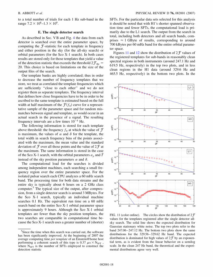
to a total number of trials for each 1 Hz sub-band in therange 7:2� 108–1:3� 109.

E. The single detector search

As described in Sec. V B and Fig. 4 the data from eachdetector is searched over the entire parameter space, bycomputing the F -statistic for each template in frequencyand either position in the sky (for the all-sky search) ororbital parameters (for the Sco X-1 search). In both casesresults are stored only for those templates that yield a valueof the detection statistic that exceeds the threshold 2F thr �20. This choice is based on limitations on the size of theoutput files of the search.

Our template banks are highly correlated; thus in orderto decrease the number of frequency templates that westore, we treat as correlated the template frequencies whichare sufficiently ‘‘close to each other’’ and we do notregister them as separate templates. The frequency intervalthat defines how close frequencies have to be in order to beascribed to the same template is estimated based on the fullwidth at half maximum of the F �f0� curve for a represen-tative sample of the parameter space and for random mis-matches between signal and template, as would occur in anactual search in the presence of a signal. The resultingfrequency intervals are a few times 10�4 Hz.

The following information is stored for each templateabove threshold: the frequency f0 at which the value of Fis maximum, the values of � and � for the template, thetotal width in search frequency bins of the points associ-ated with the maximum, the mean value and the standarddeviation of F over all those points and the value of 2F atthe maximum. The same information is stored in the caseof the Sco X-1 search, with the orbital parameters ap and �Tinstead of the sky position parameters � and �.

The computational load for the searches is dividedamong independent machines, each searching a small fre-quency region over the entire parameter space. For theisolated pulsar search each CPU analyzes a 60 mHz searchband. The processing time for both data streams and theentire sky is typically about 6 hours on a 2 GHz classcomputer.5 The typical size of the output, after compres-sion, from a single detector search is around 3 MBytes. Forthe Sco X-1 search, typically an individual machinesearches 0.1 Hz. The equivalent run time on a 60 mHzsearch band on the entire Sco X-1 orbital parameter spaceis approximately 9 hours. Although the Sco X-1 orbitaltemplates are fewer than the sky position templates, thetwo searches are comparable in computational time be-cause the Sco X-1 search uses a greater number of (shorter)

SFTs. For the particular data sets selected for this analysisit should be noted that with H1’s shorter spanned observa-tion time and fewer SFTs, the computational load is pri-marily due to the L1 search. The output from the search intotal, including both detectors and all search bands, com-prises � 1 GByte of results, corresponding to around700 kBytes per 60 mHz band for the entire orbital parame-ter space.

Figures 11 and 12 show the distribution of 2F values ofthe registered templates for sub-bands in reasonably cleanspectral regions in both instruments (around 247.1 Hz and619.5 Hz, respectively) in the top two plots, and in lessclean regions in the H1 data (around 329.6 Hz and465.5 Hz, respectively) in the bottom two plots. In the

20 25 30 35 40 45 5010

−10

10−7

10−4

2Fp(

2F)

20 25 30 35 40 45 5010

−10

10−7

10−4

2F

p(2F

)

L1

H1

20 25 30 35 40 45 50

10−5

10−3

10−7

10−9

p(2F

)

2F

20 40 60 80 100 120 140 160 180

10−5

10−3

10−7

10−9

p(2F

)

2F

L1

H1

FIG. 11 (color online). The circles show the distribution of 2Fvalues for the templates registered after the single detector all-sky search. The solid line shows the expected distribution forGaussian stationary white noise. The top two plots refer to theband 247.06–247.12 Hz. The bottom two plots show the samedistributions for the 329.56–329.62 Hz band. The expecteddistribution is dominated for high values of 2F by an exponen-tial term, as is evident from the linear behavior on a semilogscale. In the clean 247 Hz band, the theoretical and the experi-mental distributions agree very well.

5Since the time when this search was carried out, the softwarehas been significantly improved. At the beginning of 2007 theaverage computing time per template of an Einstein@home hostperforming a coherent search of this type is 0:37 s� NSFT ,where NSFT is the number of SFTs employed to construct thedetection statistic


082001-18

top two plots, the distributions of 2F values closely followthe expected p0�2F � distribution, Eq. (33). This is notsurprising in regions free of evident disturbances, as al-ready shown in [19]. Note that the highest 2F values in theclean bands (top two plots) are higher in Fig. 12 than inFig. 11. This is due to the fact that the 0.1 Hz Sco X-1search has more templates than the 0.06 Hz all-sky isolatedsearch.

F. Coincidence analysis

The next stage of the analysis compares the two lists ofvalues of 2F that lie above the threshold 2F thr � 20compiled for each detector. We require that given a tem-plate in, say, L1, there exists a template in H1 such thattheir locations in parameter space are consistent with a

physical signal having triggered them both. If this is thecase, the relevant values of the detection statistic are stored(the two filters are regarded as ‘‘in coincidence’’), other-wise they are ‘‘rejected’’ and removed from the lists. Thisprocedure is identical for both searches, but the consis-tency criteria are different due to the different signals thatare searched for. This strategy is effective at reducing thefalse alarm rate if the noise in the two data streams isuncorrelated. In practice, the data are also populated by aforest of lines present both in L1 and H1, such as 16 Hzharmonics from the data acquisition system and 60 Hzpowerline harmonics, and this procedure does not elimi-nate them. However, it does eliminate the non-Gaussianuncorrelated outliers which also are in the data. We findthat the typical sensitivity improvement in h0 resultingfrom the coincidence stage is comparable for both searchesand in the range 10%–20%, depending on the frequencysub-band.

An additional criterion to identify coincident templatescould be based on comparing the values of 2F produced bythe two filters; however, as 2F is already maximized overthe nuisance parameters and , and the integration timeof the analyses is shorter than 1 day, it is in practicedifficult to introduce an ‘‘amplitude consistency cut’’ thatis simultaneously stringent and safe. For this reason wehave not included this requirement in the coincidence stageof this search (see, however, the discussion in Sec. VI A).

The coincident templates are then sorted in order ofdescending joint significance. If we indicate with 2F L1

and 2FH1 the values of the detection statistic for a pair oftemplates in coincidence, we define their joint significanceas

s�2F L1; 2FH1� � 1� P0�2F L1�P0�2FH1�; (38)

where P0�2F �, defined in Eq. (33), is the single detectorfalse alarm probability for 2F , under the assumption thatthe noise is Gaussian and stationary. We consider the loud-est coincident template pair as that yielding the largestvalue of joint significance. In practice, in the numericalimplementation we rank events according to�flogP0�F L1�� logP0�F H1��g with logP0�F �� log�1F � �F .

In the remainder of the section we provide details on thespecific implementation of the coincidence stage for thetwo analyses.


For the isolated search the coincidence windows are1 mHz in frequency f0 and 0.028 rad angular distance inposition on the celestial sphere. These coincidence windowvalues were derived from the results of the Monte Carlosimulations described in Sec. V E. More specifically0.028 rad represents a mismatch between sky positions ofat most 1 grid point. The value of 1 mHz is derived from the

20 25 30 35 40 45 5010

−9

10−6

10−3

2F

p(2F

)

20 25 30 35 40 45 5010

−9

10−6

10−3

2F

p(2F

)L1

H1

20 25 30 35 40 45 5010

−9

10−6

10−3

2F

p(2F

)

20 40 60 80 100 120 14010

−27

10−21

10−15

10−9

10−3

2F

p(2F

)

L1

H1

FIG. 12 (color online). The circles show the distributions of2F values derived from the single detector Sco X-1 searches.The top two plots show the distributions for a clean sub-band inboth detectors, 619.0–620.0 Hz. The solid curve represents thetheoretical expected distribution. The two bottom plots show thesame distributions for the sub-band 465– 466 Hz. In this band theH1 results are dominated by large values of 2F .


082001-19

results of Monte Carlo simulations by requiring a null falsedismissal rate on the simulated sample.

As described in Sec. V D, the all-sky isolated search, ifperformed on Gaussian white stationary noise, would yieldsingle-interferometer loudest templates in 1.2 Hz sub-bands with mean 2F values of 45.7 for L1 and 41.7 forH1. The difference in these mean values is due to thedifferent data sets used for the two searches (the timespanned by the L1 data set is longer than that of the H1data set) and by the different location of the detectors onEarth and to the nonuniform antenna pattern of the detec-tors. In this search, after having excluded outliers with2F > 100, we measure mean values of the loudest tem-plates of 52.2 for L1 and 46.6 for H1.6 This corresponds toan increased level of spectral contamination in the real datawith respect to Gaussian stationary noise. This is notsurprising at all—even a simple visual inspection of thespectra reveals that they are contaminated by several‘‘lines’’ (also see the discussion in Sec. VI D in [13]).

After the coincidence step the mean value of 2F for theloudest event is 39.5 for the L1 data and 32.2 for H1. If onecompares these values with the mean values before coin-cidence, 52.2 for L1 and 46.6 for H1, one recognizes thatthe coincidence step yields an improvement in h0 sensitiv-ity of 15% and 20% for L1 and H1, respectively, [remem-ber from Eq. (35) that 2F / h2

0]. In Gaussian stationarynoise the expected improvement is 11% and 17% for L1and H1, respectively. Thus, and again not surprisingly, thecoincidence step plays a greater role on real data, which isaffected by uncorrelated non-Gaussian disturbances.

Figures 13 and 14 show the values of the detectionstatistic for the loudest events before and after coincidence,

respectively. Figure 15 shows the distributions of 2F forthe loudest coincident templates. Figure 16 shows thedistribution of loudest coincident templates over the entiresky for all the 1.2 Hz sub-bands. A higher concentration oftemplates is apparent at the poles. This is to be expectedsince the poles are the regions from where a monochro-matic signal would be received by our detectors at a nearlyconstant frequency. In other words, spectral artifacts at

200 250 300 350 400 450 500 550 600 650 700

102

104

106

f0

2F

200 300 400 500 600 700

102

103

f0

2FL1

H1

FIG. 13 (color online). These plots show loudest 2F values inthe single detector searches in each 1.2 Hz sub-band.

200 300 400 500 600 700

105

102

f0

2F

200 250 300 350 400 450 500 550 600 650 700

102

103

f0

2F

L1

H1

FIG. 14 (color online). These plots show two different viewsof the values of the detection statistic 2F of the loudest coin-cident template-couples (one for every 1.2 Hz sub-band) fromthe isolated pulsar search. The mean value between the thresholdand 2F � 100 is 39.5 for the L1 data and 32.2 for the H1 data.

20 40 60 80 100 120 140 160 1800

10

20

30

40

2F

His

togr

am

50 100 150 200

0

20

40

60

80

2F

His

togr

am

L1

H1

FIG. 15 (color online). These plots show the distributions ofthe values plotted in Fig. 14. The mean value of these distribu-tions depends on the volume of the parameter space that thesearch extends over. In this case it is the whole sky in 1.2 Hzfrequency sub-bands.

6The 2F > 100 cut has been made only when computing themean values reported above in order to eliminate large outliersthat would have dominated the mean; see Figs. 14 and 15.


082001-20

fixed frequency are consistent with sources close to thepoles, during our observation time.

2. Sco X-1

In the Sco X-1 analysis we identify coincident templatesin L1 and H1 by using the metric on the relevant parameterspace; see Sec. V D 2. A real signal, if present and ofsufficient amplitude, will trigger templates in both detec-tors. These templates will be in close proximity in parame-ter space but not necessarily identical. The procedure startsby taking each template above threshold from the L1detector and first testing for orbital parameter consistencywith templates from the H1 detector. We do this using aproperty inherent to the orbital template bank, which isschematically illustrated in Fig. 17. We know that a signalwill return at least 90% of its optimal detection statistic

when processed using the ‘‘closest’’ template (in the ab-sence of noise), where the distance between templates isdefined by the metric. We can therefore identify a rectan-gular region around the L1 filter in the two-dimensionalplane of orbital parameters. This region is easily calculatedfrom the metric used to place the templates, and we wouldexpect the true signal parameters to lie within it. We cannow repeat this process for each H1 template and construct,based on the metric associated with H1, the region coveredby the H1 filters (i.e. the filters that are associated with avalue of 2F above threshold). The test now becomes asimple matter of checking for any overlap between theregion covered by the L1 filter under scrutiny and the H1filters. Overlap implies a possible consistent signal location(in orbital parameters) capable of triggering a filter in L1and H1. In this analysis there are on average 12 orbitaltemplates in H1 that are ‘‘consistent’’ with each template inL1. The process that we have just described is then re-peated for all the L1 filters.

So far we have considered only the orbital parameters.The second stage to identify filters in ‘‘coincidence’’ is totest for frequency consistency amongst those filters thathave survived the previous test. The use of the projectedmetric described in Sec. V D 2 exploits the correlationsbetween the orbital templates and the gravitational wavefrequency to reduce the overall number of filters. Doing soallows greater differences between the true and detectedsource orbital parameters and greater differences betweenthe true and detected gravitational wave frequency. UsingMonte Carlo simulations we measured the maximum sepa-

30

210

60

240

90

270

120

300

150

330

180 0

Northen hemisphere

right ascension α

0.2

30

210

60

240

90

270

120

300

150

330

180 0

Southern hemisphere

right ascension α

FIG. 16. These figures show the location in the sky of theloudest coincident template in each 1.2 Hz sub-band. The circlesshow the templates found with the L1 search and the diamondsshow the coincident templates found with the H1 search.

Y

X

FIG. 17. Here we represent a small region of orbital parameterspace. The crosses represent orbital templates used in the L1search and the circles represent those used in the H1 search. Notethat the template orientation and spacing are not the same in eachtemplate bank. The bold� represents the location of a candidateevent in the L1 detector, and the dashed rectangle surrounding itrepresents the area within which a signal must lie if this templateis the closest to the signal. The filled circles represent thosetemplates in the H1 detector that are possible coincident candi-dates. They are identified due to the overlap between theirrespective dashed rectangular regions and the L1 candidate eventdashed region. In the S2 search there are on average 12 orbitaltemplates in H1 that are consistent with each template in L1.


082001-21

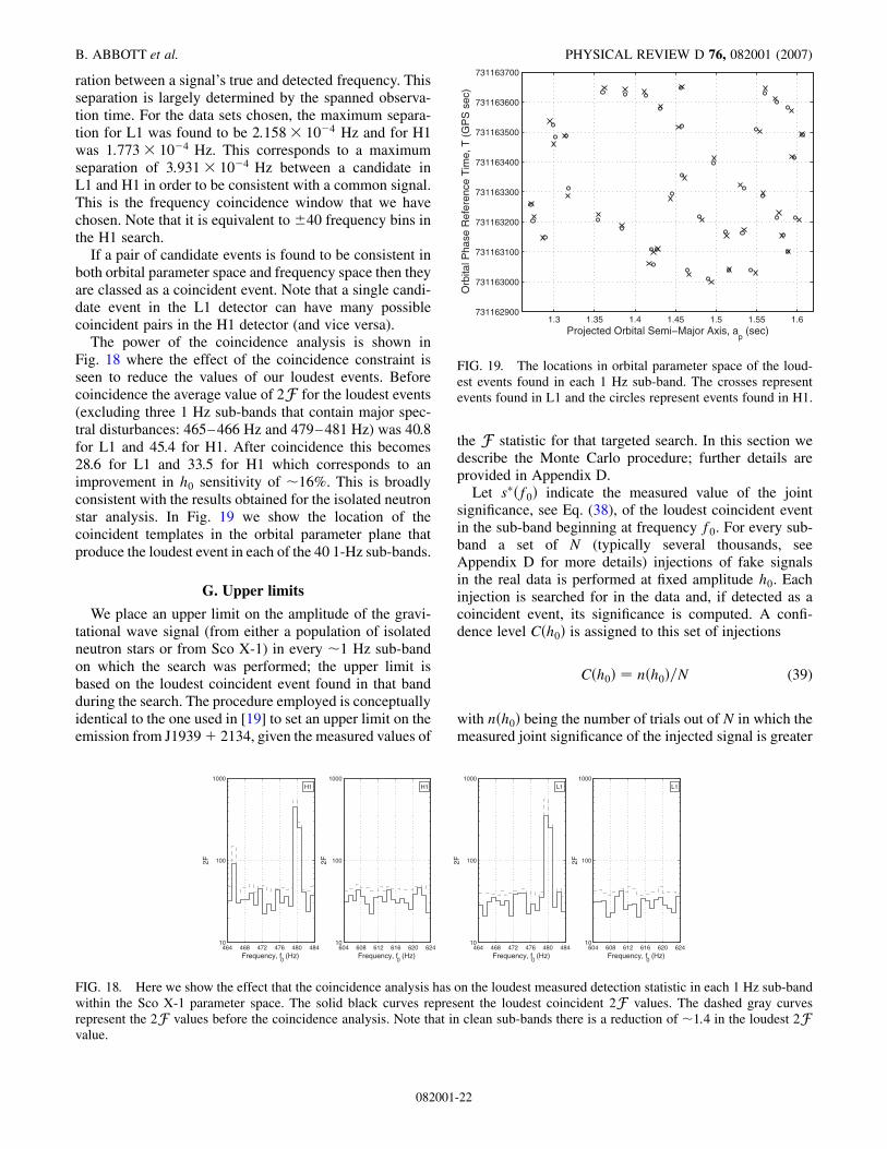
ration between a signal’s true and detected frequency. Thisseparation is largely determined by the spanned observa-tion time. For the data sets chosen, the maximum separa-tion for L1 was found to be 2:158� 10�4 Hz and for H1was 1:773� 10�4 Hz. This corresponds to a maximumseparation of 3:931� 10�4 Hz between a candidate inL1 and H1 in order to be consistent with a common signal.This is the frequency coincidence window that we havechosen. Note that it is equivalent to �40 frequency bins inthe H1 search.

If a pair of candidate events is found to be consistent inboth orbital parameter space and frequency space then theyare classed as a coincident event. Note that a single candi-date event in the L1 detector can have many possiblecoincident pairs in the H1 detector (and vice versa).

The power of the coincidence analysis is shown inFig. 18 where the effect of the coincidence constraint isseen to reduce the values of our loudest events. Beforecoincidence the average value of 2F for the loudest events(excluding three 1 Hz sub-bands that contain major spec-tral disturbances: 465–466 Hz and 479– 481 Hz) was 40.8for L1 and 45.4 for H1. After coincidence this becomes28.6 for L1 and 33.5 for H1 which corresponds to animprovement in h0 sensitivity of �16%. This is broadlyconsistent with the results obtained for the isolated neutronstar analysis. In Fig. 19 we show the location of thecoincident templates in the orbital parameter plane thatproduce the loudest event in each of the 40 1-Hz sub-bands.

G. Upper limits

We place an upper limit on the amplitude of the gravi-tational wave signal (from either a population of isolatedneutron stars or from Sco X-1) in every �1 Hz sub-bandon which the search was performed; the upper limit isbased on the loudest coincident event found in that bandduring the search. The procedure employed is conceptuallyidentical to the one used in [19] to set an upper limit on theemission from J1939 2134, given the measured values of

the F statistic for that targeted search. In this section wedescribe the Monte Carlo procedure; further details areprovided in Appendix D.

Let s��f0� indicate the measured value of the jointsignificance, see Eq. (38), of the loudest coincident eventin the sub-band beginning at frequency f0. For every sub-band a set of N (typically several thousands, seeAppendix D for more details) injections of fake signalsin the real data is performed at fixed amplitude h0. Eachinjection is searched for in the data and, if detected as acoincident event, its significance is computed. A confi-dence level C�h0� is assigned to this set of injections

C�h0� � n�h0�=N (39)

with n�h0� being the number of trials out of N in which themeasured joint significance of the injected signal is greater

464 468 472 476 480 48410

100

1000

Frequency, f0 (Hz)

2F

H1

604 608 612 616 620 62410

100

1000

Frequency, f0 (Hz)

2F

H1

464 468 472 476 480 48410

100

1000

Frequency, f0 (Hz)

2F

L1

604 608 612 616 620 62410

100

1000

Frequency, f0 (Hz)

2F

L1

FIG. 18. Here we show the effect that the coincidence analysis has on the loudest measured detection statistic in each 1 Hz sub-bandwithin the Sco X-1 parameter space. The solid black curves represent the loudest coincident 2F values. The dashed gray curvesrepresent the 2F values before the coincidence analysis. Note that in clean sub-bands there is a reduction of �1:4 in the loudest 2Fvalue.

1.3 1.35 1.4 1.45 1.5 1.55 1.6731162900

731163000

731163100

731163200

731163300

731163400

731163500

731163600

731163700

Projected Orbital Semi−Major Axis, ap (sec)

Orb

ital P

hase

Ref

eren

ce T

ime,

T (

GP

S s

ec)

FIG. 19. The locations in orbital parameter space of the loud-est events found in each 1 Hz sub-band. The crosses representevents found in L1 and the circles represent events found in H1.


082001-22

than or equal to s�. Equation (39) defines the h0 upper limitvalue as a function of the confidence C.

For every injection in a set at fixed h0 the remainingparameters are chosen randomly from within the bounda-ries of the relevant search parameter space. The errors inthe estimate of the upper limit are directly computed fromthe Monte Carlo results. Our approach typically yieldsuncertainties in the values of the upper limit of�1%–3%. An additional and larger uncertainty arisesfrom the instrument calibration, which varies with timeand depends on the detector and the frequency band. Overthe entire parameter space, we estimate that for the datasets used in the analyses presented here, the uncertaintiesamount to 11% and 9% for the isolated neutron star andSco X-1 analysis, respectively. These estimates areconservative.

The tables in [49] detail all the upper limit results. Theuncertainties associated with the upper limit Monte Carloprocedure are reported separately from the calibration un-certainties and typically they are smaller than the latter.

VI. RESULTS

In this section we present the results of the analysisperformed using the pipeline shown in Fig. 4 and describedin Sec. V. We first discuss the results regarding the all-skysearch for isolated neutron stars and then turn to upperlimits on radiation from Sco X-1.

A. Isolated neutron stars

Figure 20 shows the 95% upper limits on h0 for every1.2 Hz wide sub-band over the whole sky. The values of the

frequency refer to the lower extremum of each sub-band.(The upper limit values, along with their estimated uncer-tainties, may also be found in tabular form in [49].) Thecircles around the upper limit dots mark points in the 90thpercentile in joint significance. About 2=3 of these pointsare also in the 90th percentile for h95%

0 .About one quarter of the 90th percentile significance

points lie in sub-bands influenced by spectral disturbances(points with circles on shaded bands in Fig. 20). Most ofthe remaining points can be immediately attributed tononastrophysical sources because the ratio of theF -statistic values in the two detectors is either too largeor too small to be consistent with being due to the samesignal. These points are indicated in Fig. 20 by a square.There remain 6 points which are in the 90th percentile insignificance and cannot be excluded based on the ratios ofthe F -statistic values. They appear at the frequencies160.0 Hz, 466.79 Hz, 546.03 Hz, 564.02 Hz, 626.80 Hz,and 700.51 Hz. The 160.0 Hz frequency coincides with the10th harmonic of 16.0 Hz, a key operating frequency of thedata acquisition system. We are thus confident that theorigin of this outlier is instrumental. The points at466.79 Hz, 626.80 Hz, and 700.51 Hz are due to linesonly in the L1 instrument which have disappeared inscience runs subsequent to S2. This check suggests thatthe outliers are of instrumental origin. The 546.03 Hz and564.02 Hz points are due to lines which clearly appear onlyin H1. However, the lines are present in the S2 run and inlater science runs. The amplitude of both lines decreaseswith increasing sensitivity of the instrument, dropping by afactor of 10 (in noise power) as the sensitivity increases bya factor greater than 5. This indicates a behavior which isnot consistent with the model of the signal that we aresearching for here and suggests that these lines are ofinstrumental origin. Figure 21 shows the average powerspectral density in both detectors in the frequency regionswhere these outliers are located.

Unlike what is described in [13] no frequency band isexcluded from the upper limit analysis due to it beingcontaminated by known noise artifacts. This results inextremely loud events in some sub-bands: those containingthe 60 Hz powerline harmonics, the L1 calibration line (at167 Hz), the violin modes of the suspension wires of thetest mass (in the 340–350 Hz region) and the variousoscillator harmonics at multiples of 36 Hz together withthe beating of the 0.74 Hz pendulum mode of a test massagainst the oscillator line (in the 220–335 Hz region). Inthe case of the 179.4 Hz sub-band containing the 180 Hzpowerline harmonic, the spectral disturbance is so strongthat the upper limit Monte Carlo does not converge to anupper limit h95%

0 value. The sub-bands marked by shadedvertical stripes indicate frequencies where known spectralartifacts are present.

The upper limit values presented here are in broadagreement with what is expected and we consider this a

200 300 400 500 600 700

10−22

10−21

f0

h 095%

FIG. 20 (color online). Upper limits based on the loudesttemplate over the whole sky in 1.2 Hz sub-bands. The verticalstripes mark the sub-bands containing known spectral disturban-ces. The circles mark the 90th percentile most significant results.The squares indicate that the values of the detection statistic inthe two detectors are not consistent with what one would expectfrom an astrophysical signal.


082001-23

FIG. 21. The average power spectral density in the two detectors in the frequency regions around the five not immediately explainedoutliers from the search for isolated pulsars. The width of these disturbances is sufficiently small that they could not be discarded as ofnonastrophysical origin based on this. A peak in power spectral density is clearly visible only in one of the detectors, but the measuredvalues of the detection statistics are not inconsistent with an astrophysical signal, albeit a rare one. As explained in Sec. VI A we verystrongly suspect these excesses of power are not due to a continuous wave source because of their inconsistent amplitudes in scienceruns subsequent to S2.


082001-24

further validation of the analysis pipeline. We have run thepipeline presented here on Gaussian stationary noise andempirically derived a formula for the expected h95%

0 as afunction of the noise level in the detectors:

h95%0 � 29:5

��hShi

10 hrs

s; (40)

with hShi being the average noise level over 1.2 Hz andover the observation time in every detector and then aver-aged over the detectors: this quantity is shown in Fig. 6. Wewould like to stress that Eq. (40) refers to this particularanalysis and pipeline. The expected upper limits forGaussian stationary noise are plotted against the measuredones in Fig. 22. It is clear that in regions where the data is

not Gaussian and stationary Eq. (40) does not predictcorrectly the values that we measure and the discrepancybetween the prediction and the measured value depends onthe details of the spectral disturbance and of the methodused for estimating the noise. This is particularly evidentclose to spectral disturbances, where clearly the noise isnot white Gaussian and often not stationary and the pre-dictions can even be larger than the actually measuredupper limit value (see the points below 1 in the lowerplot of Fig. 22). However, the ratio of the measured upperlimits to the expected one never exceeds 4.4 and the 90thpercentile level in this ratio is 1.7.

B. Sco X-1

The upper limits on gravitational waves from Sco X-1are summarized in Fig. 23 (more details are provided in[49]): we show h95%

0 over 1 Hz sub-bands in the range 464–484 Hz and 604–624 Hz, assuming that the source is in anexactly circular orbit. We would like to stress that theselimits apply to a source whose orbital parameters lie in theregion reported in Table I, corresponding to 1� � errors.The typical value of h95%

0 is � 2� 10�22 over the wholeanalyzed 40 Hz band, with the exception of a band� 2 Hzaround 480 Hz which corresponds to one of the strongharmonics of the 60 Hz powerline, cf. Fig. 7. In this regionthe upper limit is h95%

0 � 10�21. Such values are consistentwith the sensitivity estimates shown in Fig. 3, which werederived under the assumption of Gaussian and stationarynoise and include a number of approximations to quantifythe effects of each stage of the pipeline considered in this

200 300 400 500 600 700

10−22

10−21

f0

h 095%

200 300 400 500 600 7000

1

2

3

4

5

6

f0

Rat

io o

f mea

sure

d up

per

limit

to e

xpec

ted

uppe

r lim

it

FIG. 22 (color online). Top plot: the circles are the upper limitsbased on the loudest template over the whole sky in 1.2 Hz sub-bands. The solid line is the expected upper limit under theassumption that the noise in the detectors is Gaussian and sta-tionary. Bottom plot: ratio of the measured upper limit values tothe expected upper limit values. The circles indicate the 90thpercentile values of the measured to expected upper limit ratio.The crosses mark the upper limit values for which the ratio of thedetection statistic values in the two detectors is not consistentwith what we would expect from a signal. In both plots theshaded regions indicate frequency bands affected by knownspectral disturbances.

464 468 472 476 480 48410

−22

10−21

f0

h 095%

604 608 612 616 620 62410

−22

10−21

f0

FIG. 23. The upper limits on the amplitude of gravitationalwave radiation from Sco X-1. The plot shows the limits on h0 at95% confidence (solid line) as a function of frequency. We reportone limit for every 1 Hz sub-band and the Sco X-1 orbit isassumed to be exactly circular. The shaded region shows thecombined errors on h95%

0 due to the injection process (typicallyin the range �2� 5� 10�24) and instrument calibration. Thelatter, estimated at the level � 9%, dominates the uncertainties.


082001-25

search. Through the statistical modelling of the pipeline weare able to express the expected h95%

0 upper limit as

h95%0 �f� � 28

��hSh�f�i6 hrs

s; (41)

where hSh�f�i is the noise level over the 1 Hz sub-bandsaveraged over the observation time, the frequency band,and the detectors.

In Fig. 24 we show the value of hC0 as a function of C forselected frequency sub-bands. We have considered both‘‘quiet’’ and ‘‘noisy’’ spectral intervals, but have restrictedthis analysis to only four 1 Hz frequency sub-bands due tocomputational burdens. Figure 24 shows that h99%

0 andh50%

0 are a factor � 2 larger and smaller, respectively,than h95%

0 .So far we have restricted the discussion of the upper

limits to the case of an exactly circular orbit. This is themodel that we have assumed in building the templates usedin the analysis. As we have mentioned in Sec. IV B 2, theorbital fits of the optical data are consistent with e � 0,which is in agreement with the theoretical expectationsinferred from evolutionary models. However, present ob-servations do not constrain the eccentricity to e & 10�4,which would introduce systematic losses of signal-to-noiseratio smaller than� 0:1, the value of the mismatch adoptedfor this search. It is therefore important to explore theconsequences of a (unlikely but possible) nonzero eccen-tricity of the Sco X-1 orbit on the results reported so far.The pipeline that we have developed allows us to quantifythis effect in a fairly straightforward way: the Monte Carlosoftware injections used to set upper limits are performedagain by drawing signals from a population of binarieswhere now the eccentricity is set to a (constant) value e �

0. The orbital parameters and the frequency are chosenrandomly exactly as in the case for a circular orbit. Wedetect the signals from eccentric orbits with the searchpipeline constructed with a bank of filters for a perfectlycircular orbital model. In this way we can quote consis-tently an upper limit on h0 for e � 0. We repeated thisprocedure for selected values of the eccentricity, e � 10�4,5� 10�4, 10�3, and 5� 10�3. The dependence of thevalue of the upper limit on h0 as a function of the con-fidence level for four representative frequency sub-bands isshown in Fig. 24 and the upper limits over the whole 40 Hzregion (at fixed confidence level) are summarized inFig. 25 and in [49]. Notice that in this case we choosedifferent values of the confidence level depending on theeccentricity of the orbit of the putative source populationused for the injection. This stems directly from the fact thatthe detection efficiency of the search pipeline is progres-sively reduced as the model of the injected signals differsmore and more from that of the detection templates. Inother words we suffer from systematic losses of signal-to-noise ratio due to the fact that the templates are notproperly matched to the signal: for e * 10�3 the fitting

factor of a filter generated by modelling Sco X-1 as acircular orbit binary is <0:9. Indeed, regardless of thestrength of the injected signals, the pipeline is unable todetect at least 95% of them, see Fig. 24. We find that fore � 10�3 and 5� 10�3 the pipeline has a maximum de-

FIG. 24. Examples of how the confidence level in the upperlimit on h0 from Sco X-1 scales with the amplitude of injectedsignals. Here we show 4 plots each corresponding to a different1 Hz sub-band. The sub-bands 464–465 Hz, 469– 470 Hz, and614–615 Hz show the confidence level across the range oftypical injected h0 values (10�22–4� 10�22). The sub-band479–480 Hz contains a large spectral disturbance and theinjections are appropriately increased in amplitude in order toachieve the required confidence level. The 5 curves in each plotrepresent the confidence level associated with different values oforbital eccentricity. The circles represent e � 0, the plussesrepresent e � 10�4, the crosses represent e � 5� 10�4, thesquares represent e � 10�3, and the triangles represent e � 5�10�3. Note that for the 6-hour observation, the pipeline is assensitive to signals with values of e < 10�4 as it is to circularorbits. For signals with e � 10�3 the pipeline has a maximumdetection efficiency of�90%–95%. For e � 5� 10�3 the maxi-mum detection efficiency reaches only �50%–70%.


082001-26

tection efficiency in the ranges �90%–95% and�50%–70%, respectively. As a consequence, for e �10�3 we report h88%

0 , and for e � 5� 10�3 we considerh50%

0 , because across each of the 1 Hz sub-bands we haveachieved at worst an 88% and 50% confidence level,respectively (see Fig. 25). On the other hand, for e � 5�

10�4 the systematic loss of signal-to-noise ratio is small oreven negligible, and we can quote upper limits at 95%confidence level. We find that, as expected, the values ofh95%

0 for e � 0 and e � 10�4 are essentially identical. Fore � 5� 10�4, h95%

0 is about 50% bigger than in the casee � 0.

Considering the limited sensitivity of the present analy-sis (see Figs. 3, 23, and 25) with respect to the astrophys-ical predictions, Eq. (24), we have not followed up (e.g.using a longer integration time Tspan) regions of the pa-rameter space that yielded particularly large values of F .Such a follow-up would be computationally very intensiveand the fact that we are targeting a continuous gravitationalwave emitter allows us to go back to the same parameterspace in the future, exploiting higher sensitivity, betterquality data, and a more sensitive search algorithm. Thiswork is already in progress. It is, however, important toestablish that the results that we have obtained do not showany obvious unexplained feature and are qualitatively con-sistent with the expectation that no signal is present in thedata set at the sensitivity level of the search. In Fig. 26 weshow the distribution of the parameters that characterizethe filters in coincidence in L1 and H1 for a representativefrequency band, 614–614.2 Hz. Because of the high cor-relation of the templates used in the analysis, one wouldexpect a cluster in parameter space of filters in coinci-dence, were a real signal present. Considering the coinci-dent filters in the three-dimensional search space �f0; ap; �T�and projecting them onto the plane �ap; �T�, no particularstructure is evident, with coincident templates evenly dis-tributed across the plane. This is also broadly consistentwith the distributions of coincident templates that we haveobtained by performing Monte Carlo simulations of theentire search pipeline on stationary and Gaussian noise.There is, however, some structure in the plane �ap; �T� thatis determined by narrow spectral disturbances and ac-counts for the large outliers in the values of the detectionstatistic at the end of the analysis pipeline. In order toexplore this, it is useful to project the same three-dimensional parameter space onto either the �f0; ap� or�f0; �T� plane. Structures are now clearly visible consistingof ‘‘stripes’’ of events at approximately (but not exactly)constant frequency. These are caused by small narrowspectral features present in the data that produce relativelylarge values of the F -statistic for a number of orbitaltemplates. Because of the short coherent integration time,such disturbances are not averaged out by the demodula-tion process and are registered in the single detector search.We find that they are very common in the output of thesingle detector search; the coincidence stage of the analysisallows those stripes of events that exist in both detectors atapproximately the same frequency to survive the entirepipeline.

We have so far reported the results of the analysis asupper limits on the signal amplitude h0. We can now recast

FIG. 25. The upper limits on h0 as a function of frequency fordifferent orbital eccentricities for the Sco X-1 search. Notice thatfor sake of clarity, we have adopted a different scale on thevertical axis than that used in Fig. 23; as a consequence the upperlimits in the frequency region 479–481 Hz are not shownbecause they are off scale. Because of the systematic loss ofsignal-to-noise ratio due to signal-template mismatch for pop-ulations of signals from sources in eccentric orbits, the con-fidence level C at which the upper limit hC0 is computed isdifferent depending on the value of eccentricity e; see text fora detailed justification. We report h95%

0 for e � 10�4, h95%0 for

e � 5� 10�4, h88%0 for e � 10�3, and h50%

0 for e � 5� 10�3.The shaded areas represent the combined errors due to theinjection process and the instrument calibration.


082001-27

them as upper limits on the ellipticity � of the neutron star,taking the distance of Sco X-1 as d � 2:8 kpc; see Table I.Using

� ’ 0:237�h0

10�24

��d

1 kpc

��1 Hz

f

�2�

1045 g cm2

Izz

�; (42)

and the canonical value for the principal moment of inertiaIzz � 1045 g cm2 we obtain:

�95% � 4:0� 10�4–3:6� 10�3 for e � 10�4; (43)

over the frequency band. The previous result can be gen-eralized to the case of a more pronounced nonzero eccen-tricity; e.g. we obtain

�88% � 5:1� 10�4–3:7� 10�3 for e � 10�3: (44)

Despite being far from astrophysically interesting,Eqs. (43) and (44) represent the first direct measurementsof the ellipticity of the neutron star in Sco X-1 in therelevant frequency band.

VII. CONCLUSIONS

We have presented here results from two wide parameterspace searches for continuous gravitational wave signals.A subset of data from the second science run of the LIGOinstruments was analyzed, the data chosen to maximize thesensitivity of the search. Two different astrophysicalsearches were performed: an all-sky search aimed at sig-nals from isolated neutron stars and an orbital parametersearch aimed at signals from the neutron star in the binarysystem Sco X-1. Both searches also cover a wide range ofpossible emission frequencies: a 568.8-Hz band for theisolated pulsars search and two 20-Hz bands for theSco X-1 search.

The sensitivity of these analyses makes the detection ofa signal extremely unlikely. As a consequence the maingoal of the paper is to demonstrate an analysis methodusing real data, with a pipeline considerably more complexthan any other coherent searches previously performed.More importantly, this coherent search will be deployedin a hierarchical analysis scheme. The first step of a hier-archical analysis sets the ultimate sensitivity of the search:candidates that do not survive the first threshold are lost. Itis thus crucial to employ the most sensitive possible tech-nique in this first step. The coherent search described inthis paper provides an implementation of such a first step.

Overall, hierarchical approaches are expected to achieveoptimal sensitivity at constrained computational resources.We will employ such approaches for deep searches on longduration and high sensitivity data such as those that arenow being recorded by the instruments. With 1 year of dataat the design sensitivity of the detectors, the improvementsthat we can expect by means of hierarchical schemes thatutilize this type of coherent analysis as one of the steps is oforder 10 with respect to what was presented here.

1.3 1.35 1.4 1.45 1.5 1.55 1.6731163000

731163100

731163200

731163300

731163400

731163500

731163600

Project Orbital Semi−Major Axis, ap (sec)

Orb

ital P

hase

Ref

eren

ce T

ime,

T (

GP

S s

ec)

614 614.05 614.1 614.15 614.2

1.3

1.35

1.4

1.45

1.5

1.55

1.6

Pro

ject

Orb

ital S

emi−

Maj

or A

xis,

ap (

sec)

Gravitational Wave Frequency, f0 (Hz)

614 614.05 614.1 614.15 614.2731163000

731163100

731163200

731163300

731163400

731163500

731163600

Gravitational Wave Frequency, f0 (Hz)

Orb

ital P

hase

Ref

eren

ce T

ime,

T (

GP

S s

ec)

FIG. 26. The locations of coincident templates within a repre-sentative subsection of the Sco X-1 parameter space. These plotscontain events found in the frequency band 614.0–614.2 Hz andare representative of a ‘‘clean’’ search band. We show onlyevents from the H1 detector for clarity (L1 coincident eventslie in approximately the same locations). We show 3 two-dimensional projections through the three-dimensional searchspace. The first plot shows the projected orbital semimajor axis,ap, versus the orbital phase reference time, �T, and shows noobvious structure. The second and third plots show ap and �T,respectively, versus f0. Here we do see structure caused by smallnarrow lines present in the data that the demodulation processhas failed to smooth out over the relatively short 6-hour obser-vation time.


082001-28

The most constraining 95% confidence level h0 upperlimit from the all-sky search is 6:6� 10�23 in the band245.2–246.4 Hz, reflecting the highest sensitivity of theinstruments at these frequencies. This is still a factor of�16 higher than the strongest signal that we expect basedon the optimistic (but not unreasonable) assumptions of thestatistical argument presented in Sec. III B 1.

The 95% confidence level upper limits from the Sco X-1search, assuming a noneccentric orbit, are h0 �2� 10�22; the most stringent 95% confidence level upperlimits from the Sco X-1 search, assuming a noneccentricorbit, are h0 � 1:7� 10�22 in the 464–484 Hz band andh0 � 2:2� 10�22 in the 604–624 Hz frequency band. TheSco X-1 results presented here are the first direct gravita-tional wave upper limits placed on the system.

Coherent all-sky searches for continuous signals fromisolated stars have been performed in the past, but overmuch smaller parameter space. In [18] an all-sky 0.76 Hzband search was performed around 921.38 Hz, includingspin-down parameters in the range �2:36� 10�8 Hz s�1

to 2:36� 10�8 Hz s�1. Three data sets, each 48-hourslong, were coherently analyzed and a 90% confidence levelupper limit was placed at the level of 1:0� 10�22 based onthe cleanest of the data sets.

In the context of a hierarchical search aimed at detectinga signal, data cleaning procedures to remove noise artifactsare likely to be employed. This is in contrast to the ap-proach used in the analysis reported in this paper where nocleaning at all was considered. Here we wanted to inves-tigate the effect of noisy data segments with a variety ofartifacts on the output of a search pipeline; we have pur-posely kept the ‘‘bad’’ data in the presentation of the resultsfor illustration purposes. This is relevant to future searchesbecause the upfront ‘‘cleaning’’ of known noise artifactsdoes not guarantee that longer observation times will notuncover unknown periodicities. These must then be eitheridentified as of instrumental origin, as done here, or fol-lowed up.

Longer observation times mean a higher resolution inparameter space and higher computational costs. It is thusimportant to lay the template banks in a way that takesadvantage of the correlations in parameter space. TheSco X-1 search presented here already does this. In futurework the metric approach will be used also for templateplacement for the searches for signals from isolatedsources. However, longer observation times and targetingdifferent LMXB systems will require more sophisticatedtemplate placement strategies than the one presented herefor Sco X-1. For example the parameter space may grow toinclude the orbital period, the eccentricity and the spinperiod derivatives. For any specific source the number ofsearch parameters will be defined by the precision to whichthese source parameters have been measured via electro-magnetic observations.

Redundant template grids produce redundant events.This increases the false alarm rate and in practice reduces

the sensitivity of the search; in fact the threshold on signal-to-noise ratio that defines the candidates to follow updepends by how many follow-ups one can afford withgiven computational resources. It is therefore importantfor future work to develop techniques to recognize non-independent candidates in parameter space, rank them, andkeep the information on only the most significant. In thispaper we have made the first moves in this direction withthe algorithm that identifies as a single candidate values ofthe F statistic which are ‘‘near’’ to each other in searchfrequency. The concept must be generalized to the multi-dimensional space of the search parameters, and ultimatelyconnected to the global properties of the detection statisticover the parameter space.

ACKNOWLEDGMENTS

The authors gratefully acknowledge the support of theUnited States National Science Foundation for the con-struction and operation of the LIGO Laboratory and theParticle Physics and Astronomy Research Council of theUnited Kingdom, the Max-Planck-Society, and the State ofNiedersachsen/Germany for support of the constructionand operation of the GEO600 detector. The authors alsogratefully acknowledge the support of the research by theseagencies and by the Australian Research Council, theNatural Sciences and Engineering Research Council ofCanada, the Council of Scientific and Industrial Researchof India, the Department of Science and Technology ofIndia, the Spanish Ministerio de Educacion y Ciencia, TheNational Aeronautics and Space Administration, the JohnSimon Guggenheim Foundation, the Alexander vonHumboldt Foundation, the Leverhulme Trust, the Davidand Lucile Packard Foundation, the Research Corporation,and the Alfred P. Sloan Foundation. This document hasbeen assigned LIGO Laboratory Document No. LIGO-P050008.

APPENDIX A: SCORPIUS X-1

In this appendix we summarize the observational resultsthat constrain the Sco X-1 parameters and provide justifi-cation for the choices made regarding the search area, seeIV B 2. We refer to Table I for a summary of the parametersof the source and the relevant errors.

In the analysis we assume the position of the source to beknown and we demodulate the data stream for that particu-lar sky location. In fact, the most accurate determination ofthe Sco X-1 sky position comes from Very Long BaselineArray observations [50,51] and is reported in Table I. Theoverall error on the source location is �0:5 arcsec, whichis significantly smaller than the �100 arcsec sky resolu-tion associated with a 6-hour GW search. Hence we as-sume the position of Sco X-1 (i.e. the barycenter of thebinary system) to be exactly known and we point (insoftware) at that region of the sky.


082001-29

We turn now to the case of the orbital parameters. In thecase of a circular binary (e � 0), three are the parametersthat describe the orbit and describe the evolution of theDoppler phase shift introduced by the binary motion: theorbital period (P), the projection of the semimajor axis ofthe orbit ap, and what we have defined as the orbital phasereference time �T, the time at which the star crosses theascending node as measured by an observer at the SSB.This is equivalent to setting the argument of periapse (theangle between the ascending node and the direction ofperiapsis) to zero.P is by far the most accurately determined parameter

[52]; for a coherent search over 6 hours it can be consid-ered known because the loss of signal-to-noise ratio (SNR)introduced by matching two templates with any value of Pin the range of Table I is negligible. P becomes a searchparameter, requiring multiple filters, only for coherentintegration times * 106 s. Much larger uncertainties char-acterize ap and �T. The large uncertainty on ap is primarilydue to the poor determination of the orbital velocity (40�5 km s�1 [53]). The uncertainty on the orbital phase refer-ence time is due to the difficulty in locating the Sco X-1low-mass companion on the orbit. The search thereforerequires a discrete grid of filters in the �ap; �T� space.

For the phase model adopted in this analysis we assumethat Sco X-1 is in a circular orbit: this is consistent withastrophysical models of semidetached binary systems andwith the best fits of the orbital parameters [42]. However,orbital fits for models with e � 0 were clearly dominatedby the noise introduced by the geometry of the Roche lobe[42]. Over an integration time of �6 h, the eccentricityneeds to be smaller than �10�4 in order for the detectionstatistic F to be affected less than 1%; for e � 10�3, lossesof the order of 10% are expected and are consistent withthe results presented in Sec VI B. Unfortunately, currentobservations are not able to constrain e to such levels ofaccuracy.

The last parameter we need to search for is the frequencyof the gravitational radiation f. The rotation frequency � ofSco X-1 is inferred from the difference of the frequency ofthe kHz quasiperiodic oscillations (QPOs). Unfortunatelythis frequency difference is not constant, and over a 4-dayobservation [54] has shown a very pronounced drift be-tween 237� 5 Hz to 307� 5 Hz, where the errors shouldbe interpreted as the 1� values [55]. This drifting of QPOfrequency separation was found to be positively correlatedto the inferred mass accretion rate. It is also important tostress that there is a still unresolved controversy as towhether the adopted model that links the rotation fre-quency to the difference of the frequency of the kHzQPOs is indeed the correct one, and if it is valid for allthe observed LMXBs. Moreover, the gravitational wavefrequency f is related to � in a different way, depending onthe model that is considered: f � 2� if one considersnonaxisymmetric distortions and f � �4=3�� if one con-

siders unstable r-modes. It is therefore clear that a searchfor gravitational waves from Sco X-1 should assume thatthe frequency is essentially unknown and the whole LIGOsensitivity band (say from � 100 Hz to � 1 kHz) shouldbe considered. Because of the heavy computational bur-den, such a search requires a different approach (a hier-archical analysis scheme, which is under development).For the analysis presented in this paper, we have decided toconfine the search to GWs emitted by nonaxisymmetricdistortions (f � 2�) and to constrain the frequency band tothe two 20 Hz wide bands (464–484 Hz and 604–624 Hz)that bound the range of the drift of �.

APPENDIX B: TEMPLATE BANKS

In Sec. V D we have described the filter banks used inthe analysis. Here we provide details about the way inwhich they were generated.


The three-dimensional parameter space is representedby right ascension and declination ��; �� that identify thesource position in the sky and the signal’s emission fre-quency. We construct a filter bank with a 10% maximummismatch. For simplicity, we employ a uniform grid infrequency, with resolution � 1=Tspan, and sky area, asdescribed in Sec. V D 1: the resulting spacing in frequencyis �f0 � 3:472� 10�6 Hz and an isotropic grid in skycoordinates with equatorial spacing of 0.02 rad, for a totalof just under 31 500 filters to cover the entire sky. Thenumber of templates in right ascension � at any givendeclination � is proportional to cos�.

The grid is chosen based on the maximum expecteddegradation in the detection statistic due to the mismatchbetween the actual position of a putative source and thetemplate grid. This effect is measured by Monte Carlosimulations. The simulations consist of series of searchesof signals at random locations in the sky with positiontemplates uniformly randomly displaced from the signal’ssource position by between 0 and half a grid step in boththe � and the � direction. We base the selection of the gridsize on the properties of the signals and the simulations aretherefore performed in the absence of noise (e.g. see [56]).The grid spacing is chosen in such a way that the expectedloss in signal-to-noise ratio due to the signal-templatemismatch is a few percent. The results are summarized inFigs. 27 and 28 that refer, respectively, to the L1 and H1data sets used in the search.

The smaller the maximum mismatch between a signaland a template the more correlated are the filters in thebank. We have estimated the effective number of indepen-dent templates from the 2F average loudest event found insingle-interferometer searches such as the one describedhere, in pure Gaussian and stationary noise in 1.2 Hz sub-bands: 45.7 for L1 and 41.7 for H1. These translate into aneffective number of independent templates which is a


082001-30

factor of �4 and �26 smaller for L1 and H1, respectively,than the actual number of templates in the sky grid that weare using for the search. The number of independent tem-plates was estimated as 1=P0�F

��, where F � is the mea-sured loudest value of the detection statistic and P0 is thefalse alarm probability defined in Eq. (33). This is consis-tent with our Monte Carlo simulations (Figs. 27 and 28)where we can see that, with the same grid, 50% of the sky is

covered in H1 with a mismatch that is always smaller than0.5% whereas in L1 50% of the sky is covered with amismatch which is about twice as large. This means thatthe grid covers H1 data parameter space with more redun-dancy than it covers L1. The main reason for the differencein coverage is the fact that the spanned observation time ofthe data set used for the L1 detector is longer than that forH1, and the resolution in sky position is highly dependenton the spanned observation time of the data set.

2. Sco X-1

In the case of Sco X-1 we search over two orbitalparameters and the gravitational wave frequency. In orderto optimally7 cover the parameter space, we consider themetric approach introduced in [48] in the context of binaryinspirals and applied to pulsar searches in [10,40]. Wedefine the mismatch between a signal, described bythe parameter vector ~ � ff0; ap; �Tg, and a template de-

scribed by ~ � ~ as8

� ~ ;� ~ � � 1�P � ~ ;� ~ �

P � ~ ; ~0�

� g�� ~ �� O�� 3�; (B1)

where the power spectrum P is given by

P � ~ ;� ~ � ��Z Tspan

0e�i��t; ~ ;� ~ �dt

��2; (B2)

��t; ~ ;� ~ � � ��t; ~ � ��t; ~ � ~ � is the differencebetween the signal and template phase and �, � � 0, 1, 2label the search parameters (we follow the convention thatthe index 0 labels frequency). The metric on the parameterspace is given by [10]

g�� h@��@��i � h@��ih@��i; (B3)

where @�� @��=@� � and is evaluated at � ~ � 0,h. . .i stands for the time average over Tspan, and the gravi-tational wave phase is defined in Eq. (29). Treating thefrequency as a continuous variable (we discuss later in thissection the consequences of the fact that the frequency is inpractice discrete) and ‘‘projecting out’’ the search fre-quency dimension of the metric yields a two-dimensionalreduced metric only on the orbital parameters,

0 0.005 0.01 0.015 0.02 0.025 0.03 0.0350

0.1

0.2

0.3

0.4

0.5

0.6

0.7

0.8

0.9

Cumulative probability distribution of 1− MisMatch: Nearest grid point

% o

f the

tria

ls o

f los

s <

x−

valu

e (#

of s

ampl

es =

1000

00)

1−Fobs

/Foptimal

FIG. 28 (color online). Fraction of trials injected in H1 wherethe ratio 1:0�F obs=F optimal is smaller than the value on thex axis. Here in this plot F obs is the F -statistic at the pointnearest to the signals’ source location. In 99% of the trials themismatch is smaller than 2%.

0 0.01 0.02 0.03 0.04 0.05 0.06 0.07 0.08 0.090

0.1

0.2

0.3

0.4

0.5

0.6

0.7

0.8

0.9

Cumulative probability distribution of 1− MisMatch: Nearest grid point%

of t

he tr

ials

of l

oss

< x

−va

lue

(# o

f sam

ples

=10

0000

)

1−Fobs

/Foptimal

FIG. 27 (color online). Fraction of trials injected in L1 wherethe ratio 1:0�F obs=F optimal is smaller than the value on thex axis. Here in this plot F obs is the F -statistic at the grid pointnearest to the signals’ source location. In 99% of the trials themismatch is smaller than 4%.

7Although we use the metric approach to lay templates in theparameter space, we use a simple square grid which is non-optimal. Using a hexagonal grid would reduce the number oftemplates by �30%.

8Note that we use the power spectrum P to define the mis-match and therefore the metric g��, but we use the F -statisticin the actual search. As the F -statistic is an optimally weightedsum of squared values of optimally weighted and summed PFTs,we would expect that the template bank is also as effective usedwith the F -statistic as for the power spectrum. This was testedwith extensive software signal injections.


082001-31

�jk � gjk �g0jgk0

g00; j; k � 1; 2: (B4)

By using the metric �jk, we take advantage of the correla-tions between the frequency and the orbital parameters—so that a mismatch in orbital parameters can be compen-sated by a mismatch in frequency—and we thereforereduce the number of orbital templates required to coverthe parameter space. In the actual analysis, we carry out acoordinate transformation from ap and �T to two ‘‘searchcoordinates’’ in order to obtain constant spacing and ori-entation of the filters over the whole parameter space,which simplifies the numerical implementation of the grid.

The frequency, however, is sampled discretely and there-fore cannot compensate exactly a mismatch in orbitalparameters: it produces a mismatch f only in f betweena template and a signal. In order to choose the appropriatefrequency spacing �f we consider the g00 component ofthe metric g��—we treat de facto f as a one-dimensionaluncorrelated dimension in the parameter space—and ob-tain

�f �2��3f

p�Tspan

: (B5)

The optimal method for dividing up the total mismatch indetection statistic is to split them up equally amongst thedimensions of a parameter space. Therefore, to achieve therequired maximal overall mismatch of 10%, we use a 6.6%mismatch in orbital templates and a 3.3% mismatch infrequency. This sets the frequency resolution to �f �1=�5Tspan�. The grid in the two-dimensional space of theorbital templates is then computed using �jk, Eq. (B4). Inpractice, the filter spacing is determined primarily by Tspan

and the grid orientation is determined by the location of thesource in its orbit during the observation, see Fig. 10;

As the grid density in the two-dimensional parameterspace �armp; �T� scales as �fmax

0 �2, where fmax0 is the maxi-

mum search frequency, we generated a different orbitaltemplate bank for each 1 Hz frequency sub-band, in orderto minimize the computational burden. This reduced by �30% the CPU time that would have been required had weused a single template bank with a maximum frequencyparameter fmax

0 � 624 Hz for the whole analysis. In sum-mary, the number of orbital templates used for each 1 Hzsub-band ranges from 3391 (6681) to 3688 (7236) in the464– 484 Hz band and from 5738 (11309) to 6107 (12032)in the 604–624 Hz band for the L1 (H1) analysis.

APPENDIX C: HARDWARE INJECTIONS

Signals can be injected into the instrument via theactuator, by physically moving the mirrors of a Fabry-Perot cavity to mimic a gravitational wave signal.Hardware injections are designed to give an end-to-endvalidation of the data analysis pipeline, including some, butnot all, components of the calibration. Toward the end ofthe S2 run, two simulated isolated pulsar signals wereinjected into the data. We denote the two pulsars P1 andP2 and give their parameters in Table II.

The data sets were prepared using the final S2 calibra-tion version [27], and consist of 17 30-minute SFTs for H1and 14 30-minute SFTs for L1. We performed a targetedsearch to look for the pulsar signals.

The results are shown in Table II. The agreement be-tween measured and expected 8NS is good. The measuredSNRs, however, are systematically somewhat larger thanexpected. This is probably due to a small systematic errorin the calibration. The differences between the expectedSNR values shown here, and those quoted in [24], ariseprimarily from differences in the lengths of observationtimes used to make the estimate. In [24], a nominal obser-vation time of 12 hours was used. This is the length of timeduring which the hardware injections were performed.Here we have used the actual science observation timewhich is shorter, reflecting science quality data and cali-

TABLE II. Parameters of the two hardware injected pulsars. See Eqs. (25) and (26) for thedefinition of the parameters. T0 is the reference time for the initial phase, in GPS seconds in theSSB frame.

P1 P2

f0 (Hz) 1279.123 457 1288.901 235_f (Hz=s) 0 �10�8

� (rad) 5.147 162 2.345 679� (rad) 0.376 696 1.234 568 (rad) 0 0cos 0 0�0 0 0T0 (sec) 733 967 667.126 112 31 733 967 751.522 490 38h0 2� 10�21 2� 10�21

SNR H1 (exp./meas.) 17=18 34=35SNR L1 (exp./meas.) 20=22 21=22


082001-32

bration quality flags based on which we discard data as notreliable enough to be included in an astrophysical search.

APPENDIX D: UPPER LIMITS

In Sec. V G we have described the method used to setupper limits in each of the �1 Hz sub-bands in which thewhole frequency bands of the two searches were divided.In this appendix we provide more technical details, on theMonte Carlo approach that we used to determine the valueof the gravitational amplitude that we report as upper limit,and the errors that affect such an estimate.

We recall that, given the value of the joint significance ofthe loudest coincident event, the upper limit on the ampli-tude hC0 at confidence level C�h0� is determined by meansof Monte Carlo simulations. In these, a set of N signals allwith the same amplitude h0 is injected in the very samedata set used in the analysis and searched for with the sameanalysis pipeline. For each set of injected signals, and aconfidence level C�h0� is assigned according to Eq. (39),which in turns defines the h0 upper limit value as a functionof the confidence level C.

The details of the Monte Carlo are as follows. For everyset of injected signals at fixed h0, the remaining parametersare chosen randomly from within the boundaries of theparameter space. These include the orbital parameters(orbital semimajor axis and orbital phase reference time)for the Sco X-1 search, the sky position for the all-skysearch, and the frequency f0 and the nuisance parameters , cos, and �0 for both searches. Uniform distributionsare used for f0 in the sub-band, between 0 and 2�, cosbetween �1 and 1, and �0 between 0 and 2�. For the all-sky search the population of injected signals is uniformlydistributed on the celestial sphere, that is to say that � isuniformly distributed between 0 and 2� and cos� uni-formly distributed between �1 and 1, with � between��=2 and �=2. For the Sco X-1 search the signal popu-lation is uniformly distributed across the two-dimensionalorbital parameter space (the parameters of which are givenin Table I). The semimajor axis is selected from within therange 1.26 to 1.62 seconds and the orbital phase referencetime is selected from within the GPS time range of731 163 028 and 731 163 626. The sky position and orbitalperiod are held fixed at values corresponding to the centerof their respective ranges (as it was done for the search).For each set of injections the orbital eccentricity is heldfixed at one of the following discrete values: e � 0:0, 10�4,5� 10�4, 10�3, 5� 10�3.

A search over the entire parameter space is not per-formed to search for every injection—it is computationallyprohibitive. Rather, the detection statistic is computed atthe nearest template grid point with respect to the injectedsignal parameters. The nearest template is chosen consis-tently with the criteria used for laying out the templatebank. For the Sco X-1 search the closest grid point isdefined by the metric governing the orbital parameter

space. For the isolated pulsar search a Euclidean measureis used. In the actual search noise might conspire to pro-duce a higher value of the detection statistic at a templategrid point which is not the nearest to the actual signal’sparameters. This means that our Monte Carlo may slightlyunderestimate the detection efficiency of the actual search,leading to an over-conservative (thus still correct) upperlimit. However, since our template bank has been chosenso that at most a few percent of the detection statistic maynot be recovered at the nearest grid point due to signal-template mismatch, we do not expect this effect to besevere. Furthermore, a detection/coincidence schemebased on the global properties of the detection statistic[57] (far from the signal’s true parameters) remains to beunderstood.

A set of injections at fixed h0 comprises at least 6000trials for the isolated pulsar search and 5000 trials for theSco X-1 search.

To determine the number of injections, several sets of10 000 isolated pulsar injections have been analyzed. Theinjections were performed at a fixed strain (h0 � 1:2�10�22) in a small band around 409 Hz, with sky locationsand nuisance parameters distributed as described above.Figure 29 shows the results of this analysis. We plot thestandard deviation on the confidence level as a function ofthe number of injections for 7 sets of injections and com-pare it with the expected values. The plots show that above5000 injections the standard deviation on the confidencelevel is less than 0.2% and in agreement with the expecta-tions even for small total number of injections.

101 102 103 104

10−3

10−2

10−1

Number of injections

Sta

ndar

d de

viat

ion

on th

e co

nfid

ence

FIG. 29. A total of 7 sets of 10 000 injections was performed ina small band around 409 Hz at a strain h0 � 1:2� 10�22. Foreach set the confidence level was estimated for different numbersof injections. The plot shows the standard deviation based on the7 estimates as a function of the number of injections. The dashedline shows the expected value of the standard deviation based onthe binomial distribution with a single-trial probability of 95.6,which corresponds to the measured mean confidence level at10 000 injections.


082001-33

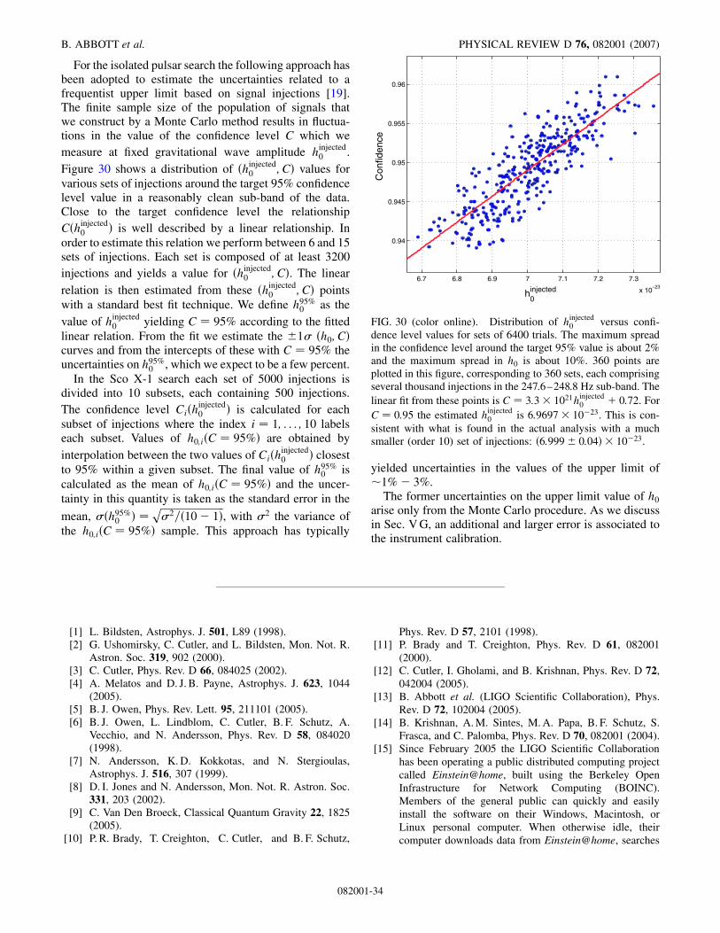
For the isolated pulsar search the following approach hasbeen adopted to estimate the uncertainties related to afrequentist upper limit based on signal injections [19].The finite sample size of the population of signals thatwe construct by a Monte Carlo method results in fluctua-tions in the value of the confidence level C which wemeasure at fixed gravitational wave amplitude hinjected

0 .Figure 30 shows a distribution of �hinjected

0 ; C� values forvarious sets of injections around the target 95% confidencelevel value in a reasonably clean sub-band of the data.Close to the target confidence level the relationshipC�hinjected

0 � is well described by a linear relationship. Inorder to estimate this relation we perform between 6 and 15sets of injections. Each set is composed of at least 3200injections and yields a value for �hinjected

0 ; C�. The linearrelation is then estimated from these �hinjected

0 ; C� pointswith a standard best fit technique. We define h95%

0 as thevalue of hinjected

0 yielding C � 95% according to the fittedlinear relation. From the fit we estimate the �1� �h0; C�curves and from the intercepts of these with C � 95% theuncertainties on h95%

0 , which we expect to be a few percent.In the Sco X-1 search each set of 5000 injections is

divided into 10 subsets, each containing 500 injections.The confidence level Ci�h

injected0 � is calculated for each

subset of injections where the index i � 1; . . . ; 10 labelseach subset. Values of h0;i�C � 95%� are obtained byinterpolation between the two values of Ci�h

injected0 � closest

to 95% within a given subset. The final value of h95%0 is

calculated as the mean of h0;i�C � 95%� and the uncer-tainty in this quantity is taken as the standard error in the

mean, ��h95%0 � �

��2=�10� 1�

p, with �2 the variance of

the h0;i�C � 95%� sample. This approach has typically

yielded uncertainties in the values of the upper limit of�1%� 3%.

The former uncertainties on the upper limit value of h0

arise only from the Monte Carlo procedure. As we discussin Sec. V G, an additional and larger error is associated tothe instrument calibration.

[1] L. Bildsten, Astrophys. J. 501, L89 (1998).[2] G. Ushomirsky, C. Cutler, and L. Bildsten, Mon. Not. R.

Astron. Soc. 319, 902 (2000).[3] C. Cutler, Phys. Rev. D 66, 084025 (2002).[4] A. Melatos and D. J. B. Payne, Astrophys. J. 623, 1044

(2005).[5] B. J. Owen, Phys. Rev. Lett. 95, 211101 (2005).[6] B. J. Owen, L. Lindblom, C. Cutler, B. F. Schutz, A.

Vecchio, and N. Andersson, Phys. Rev. D 58, 084020(1998).

[7] N. Andersson, K. D. Kokkotas, and N. Stergioulas,Astrophys. J. 516, 307 (1999).

[8] D. I. Jones and N. Andersson, Mon. Not. R. Astron. Soc.331, 203 (2002).

[9] C. Van Den Broeck, Classical Quantum Gravity 22, 1825(2005).

[10] P. R. Brady, T. Creighton, C. Cutler, and B. F. Schutz,

Phys. Rev. D 57, 2101 (1998).[11] P. Brady and T. Creighton, Phys. Rev. D 61, 082001

(2000).[12] C. Cutler, I. Gholami, and B. Krishnan, Phys. Rev. D 72,

042004 (2005).[13] B. Abbott et al. (LIGO Scientific Collaboration), Phys.

Rev. D 72, 102004 (2005).[14] B. Krishnan, A. M. Sintes, M. A. Papa, B. F. Schutz, S.

Frasca, and C. Palomba, Phys. Rev. D 70, 082001 (2004).[15] Since February 2005 the LIGO Scientific Collaboration

has been operating a public distributed computing projectcalled Einstein@home, built using the Berkeley OpenInfrastructure for Network Computing (BOINC).Members of the general public can quickly and easilyinstall the software on their Windows, Macintosh, orLinux personal computer. When otherwise idle, theircomputer downloads data from Einstein@home, searches

6.7 6.8 6.9 7 7.1 7.2 7.3

x 10−23

0.94

0.945

0.95

0.955

0.96

h0injected

Con

fiden

ce

FIG. 30 (color online). Distribution of hinjected0 versus confi-

dence level values for sets of 6400 trials. The maximum spreadin the confidence level around the target 95% value is about 2%and the maximum spread in h0 is about 10%. 360 points areplotted in this figure, corresponding to 360 sets, each comprisingseveral thousand injections in the 247.6–248.8 Hz sub-band. Thelinear fit from these points is C � 3:3� 1021hinjected

0 0:72. ForC � 0:95 the estimated hinjected

0 is 6:9697� 10�23. This is con-sistent with what is found in the actual analysis with a muchsmaller (order 10) set of injections: �6:999� 0:04� � 10�23.


082001-34

it for pulsar signals, then uploads information about anycandidates. The URL of the project is http://einstein.phys.uwm.edu/.

[16] P. Astone, K. M. Borkowski, P. Jaranowski, and A. Krolak,Phys. Rev. D 65, 042003 (2002).

[17] P. Astone et al., Classical Quantum Gravity 20, S665(2003).

[18] P. Astone et al., Classical Quantum Gravity 22, S1243(2005).

[19] B. Abbott et al. (LIGO Scientific Collaboration), Phys.Rev. D 69, 082004 (2004).




[23] B. Abbott et al. (LIGO Scientific Collaboration), Nucl.Instrum. Methods Phys. Res., Sect. A 517, 154 (2004).

[24] B. Abbott et al. (LIGO Scientific Collaboration), Phys.Rev. Lett. 94, 181103 (2005).



[27] G. Gonzalez, M. Landry, B. O’Reilly, and H. Radkins,LIGO Technical Document T040060-01-D, available athttp://admdbsrv.ligo.caltech.edu/dcc/.

[28] C. Kittel, Introduction to Solid State Physics (Wiley,Hoboken, 2005), 8th ed..

[29] N. Stergioulas, Living Rev. Relativity 6, 3 (2003).[30] R. V. Wagoner, Astrophys. J. 578, L63 (2002).[31] N. Andersson, D. I. Jones, and K. D. Kokkotas, Mon. Not.

R. Astron. Soc. 337, 1224 (2002).[32] R. N. Manchester, G. B. Hobbs, A. Teoh, and M. Hobbs,

Astron. J. 129, 1993 (2005).[33] K. S. Thorne, in Three Hundred Years of Gravitation,

edited by S. W. Hawking and W. Israel (CambridgeUniversity Press, Cambridge, England, 1987).

[34] F. M. Walter and J. Lattimer, Astrophys. J. 576, L145(2002).

[35] A. Tiengo and S. Mereghetti, Astrophys. J. 657, L101(2007).

[36] C. Palomba, Mon. Not. R. Astron. Soc. 359, 1150 (2005).[37] R. V. Wagoner, Astrophys. J. 278, 345 (1984).

[38] J. Papaloizou and J. E. Pringle, Mon. Not. R. Astron. Soc.184, 501 (1978).

[39] D. Chakrabarty, E. H. Morgan, M. P. Muno, D. K.Galloway, R. Wijnands, M. van der Klis, and C. B.Markwardt, Nature (London) 424, 42 (2003).

[40] S. V. Dhurandhar and A. Vecchio, Phys. Rev. D 63,122001 (2001).

[41] J. H. Taylor and J. M. Weisberg, Astrophys. J. 345, 434(1989).

[42] D. Steeghs (private communication).[43] The searches presented here where mainly carried out on

the Merlin cluster at the Albert Einstein Institute, theTsunami cluster at the University of Birmingham, thePleiades cluster at Penn State University, and the LDAScluster at the Hanford LIGO observatory. See http://www.lsc-group.phys.uwm.edu/lscdatagrid/.

[44] P. Jaranowski, A. Krolak, and B. F. Schutz, Phys. Rev. D58, 063001 (1998).

[45] S. D. Mohanty, Classical Quantum Gravity 19, 1513(2002).

[46] S. D. Mohanty and S. Mukherjee, Classical QuantumGravity 19, 1471 (2002).

[47] B. Krishnan, LIGO Technical Document T-040144-00-Z(2004), available at http://admdbsrv.ligo.caltech.edu/dcc/.

[48] B. J. Owen, Phys. Rev. D 53, 6749 (1996).[49] See EPAPS Document No. E-PRVDAQ-75-034712 for

tables that detail numerically the upper limit results de-scribed in the paper. For more information on EPAPS, seehttp://www.aip.org/pubservs/epaps.html.

[50] The Very Long Baseline Array Telescope, http://www.vlba.nrao.edu/.

[51] C. F. Bradshaw, E. B. Fomalont, and B. J. Geldzahler,Astrophys. J. 512, L121 (1999).

[52] E. W. Gottlieb, E. L. Wright, and W. Liller, Astrophys. J.195, L33 (1975).

[53] D. Steeghs and J. Cesares, Astrophys. J. 568, 273 (2002).[54] M. van der Klis, R. A. D. Wijnands, K. Horne, and W.

Chen, Astrophys. J. Lett. 481, L97 (1997).[55] M. van der Klis, Annu. Rev. Astron. Astrophys. 38, 717

(2000).[56] B. Owen and B. S. Sathyaprakash, Phys. Rev. D 60,

022002 (1999).[57] R. Prix and Y. Itoh, Classical Quantum Gravity 22, S1003

(2005).


082001-35

physical review d searches for periodic gravitational

Documents