1

Physical Relationship Between Reinforcement and Orientation in Clay

Nanocomposites

A. Bafna1, G. Beaucage2*, F. Mirabella3

1 Applied Extrusion Technologies Films

15 Reads Way, New Castle, DE 19720

2 Department of Material Science and Engineering

University of Cincinnati, Cincinnati, OH 45221-0012

3 Cincinnati Technology Center, Equistar Chemicals LP,

11530 Northlake Drive, Cincinnati, OH 45249

1. ABSTRACT

High density polyethylene (HDPE) nanocomposite was extrusion cast into films,

and the effect of decreasing film thickness on the orientation of intercalated clay layers is

studied. Pseudo-static tensile properties are investigated, as a function of cumulative

strain. Change in the morphology and orientation of the nanocomposite film is described

using the method of Desper and Stein for analysis of orientation in small-angle x-ray

scattering patterns. A model to relate orientation to modulus is developed and compared

to observations. The model was shown to correctly predict changes in nano-composite

properties.

Keywords: nanocomposites, orientation, mechanical properties, processing.

* To whom correspondence should be addressed [email: beaucag@uc.edu, telephone:

(513) 556-3063]

2

2. INTRODUCTION

Recently, much effort has been made towards development of polymer-clay

nanocomposites, and to understand the enhancement in properties upon addition and

dispersion of organo-clay in polymers. Reports have mentioned that orientation of the

clay layers, the polymer structures and their relative orientation with respect to each other

could play an important role in property enhancement [1-4]. A variety of processing

technologies have been explored, for example various studies have used injection

molding, due to its ability to generate a high degree of shear on the melt [1, 3, 5]. Further,

a variety of analytic techniques have been used with dynamic mechanical and tensile

properties being a few of the most commonly studied features [6-10].

Gopakumar et. al. [11] state that the PE-clay nanocomposite they studied was

exfoliated. Only a modest increase in the tensile modulus on addition of clay was

observed, which contradicts the traditional belief that exfoliated systems have maximum

property enhancement. Zhang et. al. [12] observed 20% and 40% increase in the tensile

modulus of blown polyethylene-clay films along the film machine direction (MD) and

transverse direction (TD) respectively, and qualitatively related the increase in modulus

to the orientation of the filler observed using XRD. Wang et. al. [13] showed a significant

improvement in yield strength and secant modulus in maleated polyethylene (PEMA)-

silicate (aspect ratio = 100-150) nanocomposites when compared to that in PEMA-

laponite (aspect ratio = 20-30) nanocomposites and related the improvement in the

properties to the higher aspect ratio of the filler. Using real-time, wide-angle x-ray

scattering (WAXS), Wang et. al. [14] studied the nano-scale structural changes in pure

3

PEMA and PEMA-clay nanocomposites during tensile deformation and observed that the

clay layers oriented along the tensile direction when the sample was deformed.

Liu et. al. [15] showed that increasing the filler loading in thin PP-clay

nanocomposites films, increased the storage modulus (E'), decreased the tan δ and

enhanced the rubbery plateau of E' curves. They related the enhancement in the rubbery

plateau to the enhanced stiffness of the polymer above the glass transition temperature

(Tg) due to the presence of clay. Hasegawa et. al. [16] showed that the increase in

maleated polypropylene (PPMA) to clay ratio in PP-nanocomposites increased the

storage modulus of the nanocomposite system up to 100 ºC. Similar enhancement in the

storage modulus was observed by Hambir et. al. [5] in PP-clay nanocomposite systems.

Much research [5, 11-17] has focused on relating the filler to compatibilizer ratio,

filler loading, aspect ratio, dispersion and orientation in some cases, to the property

enhancement. To further achieve a fundamental understanding of the organo-clay

reinforcement, the following question needs to be addressed.

What is the physical relationship between reinforcement and orientation in clay

nanocomposites?

A novel technique to quantitatively determine the 3D orientation of various

structures in small-angle x-ray scattering (SAXS) from a polymer-clay nanocomposite

system was developed earlier [18]. In the present study high density polyethylene

(HDPE) nanocomposites containing 5 wt % organo-clay (Cloisite 20A), 10 wt % PEMA

(2 % MA content) and 85 wt % HDPE were made. Initially a master-batch containing 10

wt % organo-clay and 20 wt % PEMA was made using a Branbury mixer. The master-

batch was then diluted by mixing it with base HDPE using a twin-screw extruder. The

4

pellets of the base resin and the nanocomposite were then extrusion cast into 1 mil, 2.5

mil, 4 mil and 8 mil thickness films. The effect of decreasing the thickness of the films,

by increasing the draw down ratio (DDR) on the orientation of clay layers was also

studied. Finally the effect of the orientation on the tensile properties of the films was

studied in order to understand the relationship between orientation and reinforcement.

3. EXPERIMENTAL

3.1 Materials

Natural montmorillonite treated with quaternary ammonium salt (Cloisite 20A,

Southern Clay Products) was used as reinforcement, maleic anhydride grafted

polyethylene (Mw = 79900 g/mol, Mw/Mn = 4.9 and MA content = 2 %) (PEMA) was

used as a compatibilizer and high density polyethylene (Mw = 139200 g/mol, Mw/Mn =

9.13, MI = 0.3 g/10min and density = 0.95 g/cc) was used as a base resin for preparing

polyethylene-clay nanocomposites.

3.2 Preparation of nanocomposite

In order to obtain a uniform mixing between the clay (powder), PEMA (pellets)

and HDPE (pellets) the pellets were ground into a 35 mesh powder using a large 1000 lb

capacity grinder. A master batch containing 10 wt. % clay, 20 wt. % PEMA and 70 wt. %

HDPE was made by melt mixing the powders in a large Banbury mixer. The clay to

compatibilizer ratio was 1:2. The temperatures in the mixer varied from 177-200 ºC and

the rotor speed was set at 120 rpm. The partially melted mixture from the mixing zone of

the Banbury mixer was extruded into thin strands using a single screw extruder and then

5

pelletized. The temperatures in the extruder varied from 172-207 ºC and the screw speed

was set at 18 rpm.

The pellets of the master batch, were then let down into HDPE using a Berstorff

twin screw extruder. Two different nanocomposite HD305 and HD510, with organo-clay

loading of 2.5 wt. % and 5 wt. % and compatibilizer loading of 5 wt. % and 10 wt. %

respectively, were made from the master batch by varying the weight % of the master

batch in the let down. HDPE containing no clay and compatibilizer, HD000, was also

passed through the twin-screw extruder and pelletized in order to maintain similar

processing history on all the resins. The temperature in the extruder varied from 182-207

ºC from zone 1 to zone 9 and was 188 ºC in the die. The screw speed was maintained at

195 rpm. The nanocomposites were extruded into thin strands and then finally pelletized.

3 Extrusion film casting

Resin HD000 and HD510 were cast into films using an extrusion cast line fitted

with a coat-hanger die of 20 mil (0.49 mm) die gap. The temperature in the extruder

varied from 180-185 ºC from zone 1 to zone 4 and was 189 ºC in the die. The cast drum

temperature was 32 ºC. The screw speed was maintained at 190 rpm. From each resin,

four different films varying in thickness were made by changing the draw down ratio

(DDR) from 20:1, 8:1, 5:1 and 2.5:1 to obtain films with thickness varying from 1, 2.5, 4

and 8 mil respectively. The effect of varying the DDR on the orientation of clay in these

films and its effect on the properties was studied.

6

3.4 Characterization

SAXS 2D measurements were conducted using an x-ray instrument described

previously [18] in order to relate the orientation of the modified clay structures to

property enhancement in the nanocomposite films. The 2D measurements are useful in

determining both size and relative orientation of modified clay and polymer lamellae

structures in the polymer-clay nanocomposite films. The films were laid over one

another, to form a 2 mm thick stack, for measurement. Care was taken that the films were

stacked in such a manner that all the films in a stack had their machine direction (MD),

transverse direction (TD) and normal direction (ND) aligned.

The tensile properties of the films along the MD were studied. The tensile

strength and elongation at yield was obtained in accordance to ASTM D882 and 1%

secant modulus was obtained in accordance to ASTM E111 using a Sintech1S universal

tensile testing machine.

4 RESULTS AND DISCUSSION

4.1 2-d Small angle x-ray scattering (SAXS)

4.1.1 SAXS analysis

Insert figure 1.

Insert figure 2.

In order to study the 3D orientation of various structures in the nanocomposite

films, x-ray measurements need to be carried out for at least two orientations of the

7

sample with respect to the x-ray beam as shown in figure 1 and described earlier [18].

Projections are designated by the three principal sample axes, M, machine direction, T,

transverse direction and N, normal direction. Corrected 2D SAXS patterns for the

different orientations are shown in Figure 2. The sample orientations are designated with

reference to Figure 1.

Insert figure 3.

For the TN and MT orientations, the azimuthal average of the 2D patterns (figure

2) yield figure 3 [18], a radial plot showing the intensity versus scattering vector q. The

d-spacing is calculated using the radial plot and Bragg’s law, d = 2π/qN*, where qN* is

the value of q at maximum intensity in a Lorentizian corrected SAXS pattern of Iq2 vs. q

(not shown). SAXS data was corrected by subtracting an empty camera background. The

radial plots give data on periodicity (dispersion) of a) intercalated clay platelet (002)

planes and b) polymer lamellae (001) planes similar to [18].

Insert figure 4.

For the MN and MT orientations the radial average of the 2D patterns yield figure

4, showing intensity as a function of azimuthal angle (φ) similar to [18]. For each sample

orientation, azimuthal plots for intercalated clay and polymer lamellar can be made.

Figure 4 compares the orientation data obtained from SAXS for the intercalated clay

8

platelets films HD510 CF 1 and HD510 CF 8. The azimuthal plots for films HD510 CF

2.5 and HD510 CF 4 lie between those of films HD510 CF 1 and HD510 CF 8 and were

not plotted in figure 4 for the reasons of clarity. For any periodic structure, the sharpness

of the azimuthal peak reflects the extent of orientation.

In the analysis of orientation in polymer samples using SAXS many authors make

the assumption of fiber symmetry and calculate the Hermans orientation function, f, using

the <cos2φ> from equation 1a [19].

( )( ) ( )

( )MMM

MMMM

M

dI

dI

!!!

!!!!

!"

"

sin

sincos

cos2

0

2

2

02

#

#= (1a)

Since uniaxial symmetry is not a general condition and since the samples studied in this

paper most likely did not display uniaxial symmetry (fiber symmetry) we have adopted

the approach described in [18] which uses equation 1b to calculate the mean <cos2φ> for

a projection in the plane of observation.

( )( ) ( )

( )MNMN

MNMNMN

MN

dI

dI

!!

!!!

!"

"

#

#=

2

0

2

2

02

cos

cos (1b)

For example if the x-ray beam is normal to the MN plane of the film, <cos2φMN> for the

MN projection can be determined using equation 1b. Through measurement of two such

projections the 3d orientation function can be determined. (This is fairly similar to

considering two projections in a mechanical drawing to determine the 3D orientation and

structure of an object.) Lindenmeyer and Lustig [20] and Buckley Crist [21] have

9

pointed out the limitations of using orthogonal projections to obtain 3d orientation from

diffraction measurements. These limitations are weakened in small angle x-ray scattering

measurements as explained in [22].

Insert table 1.

The φMN value from orientation MN along with either the φTN value from

orientation TN, or φMT value from orientation MT are used to determine the 3D

orientation of the structural normals to the intercalated clay layers, or polymer lamellar

planes, in the three principle film axes represented by φM, φT and φN using the

calculations presented in the appendix. Values of the angle and the cosine square of the

angle made by the normal of the intercalated clay platelet (002) planes and polymer

lamellar (001) planes, with MD, TD and ND of all nanocomposite films is presented in

table 1.

Insert figure 5.

The average cosine square projection of the structural normals from the ‘i’ axis,

<cos2φi>, can be used in a Wilchinsky triangle [23, 24] (Figure 5). This ternary plot,

developed by Desper and Stein [23], graphically displays the average direction of the

structural normal orientation with a single point. The Wilchinsky triangle is constructed

by counting from the opposite side of a direction ‘i’ the value of < cos2φi> and making a

10

point where the three <cos2φi> values intersect. For a randomly oriented sample

<cos2φM> = <cos2φN> = <cos2φT> = 0.333 and a point in the center of the Wilchinsky

triangle results. For perfect orientation of a plane in MT the normal points in the N

direction and a point at the ND corner results. As compared to a pole figure, a Wilchinsky

triangle is much simpler to construct, understand and interpret. As compared to

qualitative data obtained via a pole figure analysis, a Wilchinsky triangle would provide

quantitative data on the degree of orientation of different structures in a single plot.

4.1.2 SAXS results

The radial plot (figure 3) shows that the polymer lamellar long period in all the

nanocomposite films remain unchanged (L = 209 Å). The intercalated clay platelet d-

spacing (figure 3) also remained unchanged (dc = 31 Å) for all the nanocomposite films.

This indicates that varying the processing conditions did not have an effect on the

dispersion of the modified clay layers in the polymer matrix.

The 2D SAXS patterns also show that for HD510 CF 1, the intercalated clay

platelets also lie with their normal strongly oriented along the film normal direction. This

observation is consistent with those made in earlier studies [8, 18, 25-26]. The

Wilchinsky triangle shows the orientation of the intercalated clay platelet normal

orientation along the three film axes (ND, MD and TD) for all four nanocomposite films.

For a particular organic or inorganic structure, a point closer to the ND corner in the

Wilchinsky triangle indicates a higher degree of orientation of the normal to that structure

along the ND.

11

The Wilchinsky triangle shows that the intercalated clay platelet normals in

HD510 CF 2.5 (solid circle in figure 5) have lower orientation along ND as compared to

HD510 CF 1 (solid vertical double triangle in figure 5), but higher then that in HD510 CF

4 (solid triangle in figure 5) and HD510 CF 8 (solid horizontal double triangle in figure

5). Thus intercalated clay platelets normal in HD510 CF 1 have the highest orientation

while those in HD510 CF 8 have the lowest orientation along the film ND (figure 4 and 5

and table 1). Therefore an increase in the degree of orientation of intercalated clay

platelet normals along the film ND is observed in the nanocomposite films with

decreasing thickness or with increasing draw-down ratio (DDR). On a Wilchinsky

triangle, the line ( _ _ _ ) parallel to the MN plane represents points with constant

orientation along film TD. From figure 5 it is seen that the markers of the intercalated

clay platelet normal orientation for the different films lie on the line ( _ _ _ ) parallel to

the MN plane. This indicates that the orientation of the intercalated clay platelet normals

along the film TD remains almost the same for all the 4 films irrespective of the thickness

and therefore the increase in the orientation along the film ND with decreasing film

thickness is at the cost of the decrease in orientation along the film MD.

On a Wilchinsky triangle, any points that lie on the line ( ___ _ ___ ) that bisects

the NT plane would represent equal orientation along film ND and the TD. The markers

on the Wilchinsky triangle for the polymer lamellar normal orientation in the films fall on

the line bisecting the NT plane. This indicates that the increase in orientation of the

lamellar normals along the film MD with decreasing film thickness is at the cost of

decrease in the orientation equally along the film TD and ND irrespective of the initial

film thickness. Such observation of the increase in polymer lamellar normal orientation

12

along the film MD with increasing DDR in HDPE films has been reported earlier [27,

28].

The difference in the morphology of the nanocomposite films with varying DDR

could be explained based on the stress in the film at solidification. During the extrusion

film casting process the polymer melt is pushed through the die. After the melt comes out

of the die in the form of a film, it is pulled by the chill roll on which the film

crystallizes/solidifies. The part of the film between the die lip and the point where it first

touches the chiller roll is still in a partly melted state (uncrystallized) and can undergo

significant deformation on application of stress [27]. Keeping the extrusion rate (extruder

output) constant and increasing the chiller roll rotational speed, i.e. increasing the DDR,

decreases the thickness of the film. This increase in DDR could develop stresses [29] in

the part of the film between the die lip and the chiller roll, due to which the polymer may

undergo deformation along the film pulling direction (MD). This deformation increases

with increasing DDR. Due to this deformation along the MD, the polymer chains orient

along the MD. Due to the chain folding mechanism of the polymer chains in the polymer

lamellae, the polymer lamellar normal orients along the film MD and this orientation

increases with increasing DDR or decreasing film thickness. Therefore, the observation

of increase polymer lamellar normal orientation along the film MD, with increasing DDR

or decreasing film thickness, in the present study, is consistent with those made before

[27-28].

The orientation of the intercalated clay layer normals along the film ND could be

due to the tendency of the clay layers to orient with elongation along the film MD. On

13

increasing the DDR, the deformation of the polymer along the MD increases which in

turn could orient the clay basal planes along the film MD.

4.2 Mechanical properties

Insert table 2.

Insert figure 6.

Figure 6 plots inverse of film thickness (1/t) against % increase in tensile strength

at yield of the nanocomposite films over films without clay. From figure 6 and table 2 it

is seen that the value of % increase in the tensile strength at yield increases linearly with

the inverse of film thickness (1/t).

From the SAXS orientation data (table 1) it was observed that the angle (<ΦM>)

between the normal to the intercalated clay platelet and the film MD decreases with

increasing film thickness or decreasing DDR. Since in the tensile measurements, the

films were pulled along the film MD, the rise in the % increase in tensile strength at yield

could be due to the increased orientation of the clay basal plane along the film MD. From

the SAXS orientation data (table 1) it was seen that the normal to the basal plane of the

intercalated clay layers in the 8 mil film is inclined on average by 62º to the film MD or

in other words the clay basal planes are inclined on average by 28º to the film MD. This

average angle of the clay basal planes with the MD decreases to 25º, 22º and 20º in the 4,

2.5 and 1 mil films respectively. This decrease in the average angle between the clay

basal planes and the film MD with decreasing film thickness (or increasing 1/t) indicates

14

increasing reinforcing ability of the clay layers and hence an increase in the value of %

increase in tensile strength at yield. Although Brune et. al. [30] recently developed

models and predicted that the relative modulus of the nanocomposite with respect to the

base resin would increase with increasing orientation of the clay basal plane normal along

the ND; this is the first study that quantitatively determines the 3D orientation of clay

platelets and then relates the intercalated clay platelet 3D orientation to resulting property

enhancement.

Insert figure 7.

The percent increase in secant modulus is plotted against the inverse of film

thickness (1/t) in figure 7. From figure 7 and table 2 it is clear that the film 1 % secant

modulus increases linearly with the decrease in film thickness up to 2.5 mil film

thickness. Decreasing the thickness below 2.5 mil is seen to slightly increase the 1 %

secant modulus.

Experimental data on the variation of tensile modulus with the degree of

orientation of intercalated clay layers in the nanocomposite films can be used to develop

a theoretical model to predict the tensile modulus of a nanocomposite system depending

on the clay platelet orientation, next section.

4.4 Model for predicting the elastic modulus of a nanocomposite and comparison of these

values to those obtained experimentally

15

Einstein’s equation for the macroscopic viscosity, η', of the suspension of solid

spheres is written as follows [31].

η' = η (1 + 2.5 Φ) (3)

where η is the viscosity of the solvent and Φ is the volume fraction of the solid spheres in

the suspension.

For a suspension of asymmetric particles the viscosity would depend on the

orientation of the particles with respect to the flow direction. Due to this dependence of

the viscosity of the suspension on the orientation of the particles, Simha [32-33] modified

the Einstein’s equation for a suspension containing asymmetric particles. The equation

proposed by Simha [32-33] for the macroscopic viscosity, η', of the suspension of

asymmetric particles is written as follows.

η' = η (1 + ν Φ) (4)

where, ν according to equation 4 for solid spheres is 2.5, and is larger for asymmetric

particles. For disc-shaped particles ν is written as follows [33].

ν = A / tan-1(A) (5)

16

where, A is the aspect ratio, i.e. ratio of the diameter (D) to the thickness (L), of the disc-

shaped particle. Inclusion of ν (ν > 2.5) along with the volume fraction Φ in the

Einstein’s equation could mean that the presence of asymmetric particles in a suspension

possibly increases the effect of the volume fraction on the viscosity of the suspension as

compared to that by the presence of spherical particles of same volume fraction. This

behavior of asymmetric particles can be explained as follows:

ν is approximately proportional to the aspect ratio as seen in equation 5 and so it

can be written as ν ~ A = D / L. The volume fraction of the filler is Φ~D2 L N / V where,

N is the number of asymmetric particles, V is the total volume of the suspension and D

and L are the diameter and thickness of the filler respectively. Product of Φ and ν yields

ν* Φ ~ D3N / V which is the volume fraction of spheres of diameter D in a suspension.

The product of ν and Φ in equation 4 therefore enhances the effect of volume fraction on

the viscosity of the suspension since the asymmetric particles of diameter D behaves as

having occupied a volume equal to that which would have been occupied by spheres of

the same hydrodynamic diameter (figure 8).

Insert figure 8.

A parallel between hydrodynamic viscosity and Young’s modulus has been drawn

earlier in order to predict the modulus of a composite [34-41]. Based on this and equation

5, the modulus of a composite containing asymmetric filler can be written as

Ec = Em (1 + ν Φ) (6)

17

Here Ec is the modulus of a composite and Em is the modulus of the matrix polymer. If

the filler particle is sufficiently rigid then ‘ν’ has the same numerical value for equations

5 and 6 [36-41].

The modification made by Simha to Einstein’s equation, in order to account for

the asymmetric nature of the filler, assumes random orientation of the filler. Asymmetric

particles have a tendency to orient with shear due to their higher aspect ratio. In our study

on polyethylene-clay nanocomposites we determined that the tensile modulus of the

composite depends on the orientation of the filler particles along the tensile direction. For

this reason some modifications must be made to equation 6 so as to be able to predict the

modulus of the nanocomposite based on the orientation of clay layers in the polymer

matrix as measured by SAXS. Boccaccini et. al [42] had introduced a <cos2φ> term,

where φ is the angle between the rotational axis of an asymmetric particle and the stress

direction, in the equation relating the elastic modulus of a composite to that of the

polymer matrix. Using a similar approach, the Herman’s orientation function [18], f, of

the filler in the polymer matrix, was introduced to equation 6 in our study. The modified

equation for the modulus of the composite is now written as follows.

Ec = Em [1 + ν Φ/ (1-f)] (7)

Here f is the orientation function for the clay layers in the polymer matrix and is written

as shown in equation 8.

18

f = (3<cos2φ> -1)/2 (8)

where, φ is the angle between the clay basal plane and the tensile direction. Orientation

function, f, varies from 1 for perfect orientation to -0.5 for perpendicular orientation. The

reason for the inclusion, and the role played by the orientation function can be explained

as follows:

Insert figure 9.

For a composite system, the mean chord length of the filler along a particular direction

can be obtained by drawing a line parallel to that direction through the schematic of the

composite. For a composite containing uniform distribution of spherical filler particles,

the mean chord length of the filler along any direction is equal (figure 9a). For a

composite with uniform distribution of asymmetric filler particles, the mean chord length

of the filler along a particular direction depends on the orientation of the filler along that

direction (figure 9b). The addition of the orientation function term along with the filler

volume fraction term in equation 6 takes into account the mean chord length of the filler

along the stress direction and thus helps to predict the tensile modulus of a

nanocomposite system based on the direction and the degree of orientation of the clay

platelets in the polymer matrix.

Equation 7, which relates the modulus of the composite to that of the polymer

matrix, was further modified, in our study, to compensate for the confinement of polymer

between the clay galleries. The increase in the volume of the modified clay on mixing

19

with the polymer indicates intercalation of the polymer into the clay galleries. It is

believed that this intercalated polymer does not contribute towards the modulus of the

polymer and so a factor, 0.1*Em, is subtracted from equation 7, which is now written as

follows.

Ec = Em [1 + ν Φ/ (1-f)] – 0.1*Em (9)

When the clay basal planes are perfectly aligned along the tensile direction, then

the value of the orientation function is equal to 1 and equation 9 predicts very high value

of composite modulus. When the clay basal planes make an angle higher than 40º with

the tensile direction the value of the composite modulus predicted by equation 9 is lower

then that of the polymer matrix. Due to this, equation 9 is valid only for a limited range

(5º-40º) of the angle between clay basal planes and tensile direction.

The feasibility of using equation 9 for predicting the elastic modulus of the

nanocomposite films with known orientation functions is discussed below.

Insert table 3.

The aspect ratio, A, from table 3 when substituted in equation 5 gives ν = 3.99.

Substituting this value ν and the value of Φ from table 3 in equation 9 and varying the

value of orientation function, f, from 1 for perfect alignment of clay basal planes along

the tensile direction and 0 for random orientation gives Ec/Em for different values of ‘f’.

20

Insert figure 10.

Experimentally determined values of Ec/Em for the known value of orientation

function, f, for the 4 different nanocomposite films studied, are plotted against the

theoretically predicted values of Ec/Em in figure 10. Although from figure 10 it is seen

that that equation 9 roughly predicts values of Ec/Em close to those determined

experimentally the orientation and Ec/Em data obtained for just 4 different films possibly

is not enough to check the validity of equation 9.

5. CONCLUSION

High density polyethylene (HDPE) nanocomposite was extrusion cast into films,

and the effect of decreasing film thickness on the orientation of intercalated clay layers is

studied. The orientation of intercalated clay platelet normals and polymer lamellar (001)

plane normals in the nanocomposite films increased along the film ND and MD

respectively with decreasing thickness or increasing draw down ratio (DDR).

Pseudo-static mechanical properties of all the films were studied and related to the

intercalated clay platelet orientation. % Increase in the tensile strength at yield and %

increase in secant modulus for the nanocomposite films increased monotonically with

decreasing film thickness (or increasing 1/t), indicating increased reinforcement with

decreasing film thickness. Change in the morphology of the nanocomposite films with

decreasing film thickness was discussed. A model to theoretically predict the tensile

modulus based on the degree of platelet orientation was developed and compared to data.

21

In all 4 nanocomposite films the intercalated clay platelet dispersion remained the

same while their degree of orientation along the film MD varied considerably. Significant

difference observed in the tensile properties of the nanocomposite films, of different

thickness, indicated the importance of considering the orientation of the clay layers along

with its dispersion for understanding the structure property relationship in polymer-clay

nanocomposite systems. Although Brune et. al. [30] recently developed models and

predicted that the relative modulus of the nanocomposite with respect to the base resin

would increase with increasing orientation of the clay basal plane normal along the ND,

our study is the first of its kind to experimentally prove the relationship between

processing condition, orientation, and the tensile properties.

6. APPENDIX

6.1 Calculation of φM, φT and φN from φMN and φTN

Insert figure 11

Figure 11 schematically shows the three observed projections and orientation

angles obtained from the 3-d orientation of the structural normal vector from the

scattering, q. To determine the average angle of tilt of the intercalated clay platelet

normals with the MD, TD and ND (φM, φT and φN respectively) only 2 of the 3

orientations (figure 11) are needed. Since the intercalated clay platelet reflection is

clearly seen in orientation MN and TN, values of φMN and φTN are used for calculating φM,

φT and φN.

22

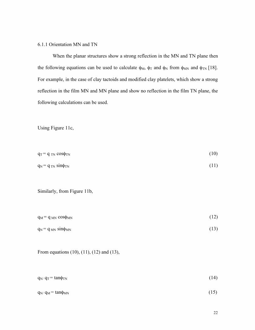
6.1.1 Orientation MN and TN

When the planar structures show a strong reflection in the MN and TN plane then

the following equations can be used to calculate φM, φT and φN from φMN and φTN [18].

For example, in the case of clay tactoids and modified clay platelets, which show a strong

reflection in the film MN and MN plane and show no reflection in the film TN plane, the

following calculations can be used.

Using Figure 11c,

qT = q TN cosφTN (10)

qN = q TN sinφTN (11)

Similarly, from Figure 11b,

qM = q MN cosφMN (12)

qN = q MN sinφMN (13)

From equations (10), (11), (12) and (13),

qN/ qT = tanφTN (14)

qN/ qM = tanφMN (15)

23

qM/ qT = tanφTN / tanφMN (16)

From Figure 11,

cos2φM = qM2/ q2 = qM

2 /(qM2 + qN

2 +qT2) (17)

cos2φN = qN2/ q2 = qN

2 /(qM2 + qN

2 +qT2) (18)

cos2φT = qT2/ q2 = qT

2 /(qM2 + qN

2 +qT2) (19)

Substituting (14), (15) and (16) in equations (17), (18) and (19) and substituting A =

tan2φTN and B = tan2φMN

cos2φM = A2/ (A2 + A2B2+ B2) (20)

cos2φN = A2B2/ (A2 + A2B2+ B2) (21)

cos2φT = B2 / (A2 + A2B2+ B2) (22)

In this way values of φTN and φMN and φMT yield the values of cos2(φM), cos2(φT) and

cos2(φN) for the normals to the intercalated clay platelets. These cos2(φi) values are

numerically derived from the mean values of the type value <cos2(φMN)> and represent a

type of average value.

24

7. ACKNOWLEDGEMENT

The authors gratefully acknowledge Equistar Chemicals LP, Cincinnati, OH for

providing the raw material and allowing us to use their resources for making the

nanocomposites and nanocomposite films. The authors thank Fred Boldt (Equistar

chemicals) for providing useful information and Jim Brooks, Katie Schroeder and Christ

Blyth (Equistar chemicals) for their help while making samples. Equipment used in this

project and G. Beaucage were supported by the National Science Foundation under

grants CTS-9986656 and CTS-0070214.

25

8. REFERENCES

1. Varlot K.; Reynaud E.; Vigier G.; Varlet J. J Polym Sci Part B: Polym Phys

2002, 40, 272-283.

2. Fornes T. D.; Yoon P. J.; Keskkula H.; Paul D. R. Polym 2001, 42, 9929-9940.

3. Kojima Y.; Usuki A.; Kawasumi M.; Okada A.; Kurauchi T.; Kamigaito O.; Kaji

K. J Polym Sci Polym Phys 1995, 33, 1039-1045.

4. Krishnamoorti R.; Yurekli K. Current Opinion in Colloid Interface Sci 2001, 6,

464-470.

5. Hambir S.; Bulakh N.; Kodgire P.; Kalgaonkar R.; Jog J. J Polym Sci Part B:

Polym Phys 2001, 39, 446-450.

6. Oya A.; Kurokawa Y.; Yasuda H. J Mater Sci 2000, 35, 1045-1050.

7. Beyer G.; Eupen K. In Nanocomposites 2001, Proceedings of the Annual

Conference, Chicago, IL, 2001.

8. Gilman J .W. Appl Clay Sci 1999, 15, 31-49.

9. Kojima Y.; Usuki A.; Kawasumi M.; Okada A.; Kurauchi T.; Kamigaito O. J.

Appl Polym Sci 1993, 49, 1259-1264.

10. Messermith P.; Giannelis E. J Polym Sci Part A: Polym Chem 1995, 33, 1047-

1057.

11. Gopakumar T. G.; Lee J. A.; Kontopoulou M.; Parent J. S. Polymer 2002, 43,

5483-5491.

12. Zhang Q.; Wang Y.; Fu Q. J Polym Sci Part B: Polym Phys 2003, 41, 1-10.

13. Wang K. H.; Koo C. M.; Chung I. J. J Appl Polym Sci 2003, 89, 2131-2136.

26

14. Wang K. H.; Choi M. H.; Koo C. M.; Xu M.; Chung I. J.; Jang M. C.; Choi S. W.;

Song H. H. J Polym Sci Part B: Polym Phys 2002, 40, 1454-1463.

15. Liu X.; Wu Q. Polym 2001, 42, 10013-10019.

16. Hasegawa N.; Kawasumi M.; Kato M.; Usuki A.; Okada A. J Appl Polym Sci

1998, 67, 87-92.

17. Varlot K.; Reynaud E.; Kloppfer M.; Vigier G.; Varlet J. J Polym Sci Part B:

Polym Phys 2001, 39, 1360-1370.

18. Bafna A. A.; Beaucage G.; Mirabella F.; Mehta S. Polym 2003, 44, 1103-1115.

19. Roe R. J. In Methods of X-ray and Neutron Scattering in Polymer Science; Eds.;

Oxford University Press, New York, 2000; Chapter 3, pp 119-127.

20. Lindenmeyer P.; Lustig S. J Appl Poly Sci 1965, 9, 227-249.

21. Buckley C.; Personal communication, 2004

22. For a SAXS measurement where a correlated (that is stacked planes) and oriented

structure is observed, the scattered intensity, I(q*, φ M), at the correlation peak q*

and azimuthal angle φM, relative to the sample's machine direction, MD, is related

to structures which meet a set of strict conditions: a) Bragg condition (having to

do with d-spacing and yielding the radial q*), b) Orientation of the stacked planes

with respect to the incident beam such that the specular condition is met (having

to do with orientation of the stacked planes at a fixed angle of half of the Bragg

angle relative to the incident beam) and c) Orientation of the plane normal at the

azimuthal angle, φM, relative to the sample's machine direction. If the assumption

of axial symmetry about the MD direction is not used, the meaning of an average

<cos2φMN> can be considered using equation 1b. For small angle scattering

27

<cos2φMN> in equation 1b reflects contributions from planes whose normals are

oriented at a small angle, θ/2 (where θ is the scattering angle), relative to the

sample plane. If an error in orientation of θ/2 can be accepted, in terms of the

application, then we can consider equation 1b as reflecting the projection of

orientation in the sample plane. For polymer samples and scattering angles less

than 6° (θ/2 < 3°) the assumption is appropriate and greatly simplifies the

quantitative description of orientation. That is, an error in orientation of less than

3° is generally not important to polymer samples especially when the Wilchinsky

approach is used to map orientation in terms of <cosφ2> (this would equal an error

of about 0.3 % of the axis on the Stein-Desper-Wilchinsky plot [23], i.e. smaller

than the symbols used to plot). The assumption becomes better than this worst

case scenario for SAXS where the value of q* is low. Additionally, since

orientation generally displays a broader distribution in direction for larger

structures, the approximation is further supported for the large structures observed

at small q. This assumption is strong for all of the small-angle regime since one

always deals with systems where < 0.3 % error is insignificant in terms of the

Wilchinsky triangle analysis. For scattering at 20° in the diffraction regime the

assumption becomes weaker with a necessary window of orientation of 10° and

an acceptable error in the Wilchinsky triangle of 3 %. The full description of this

approximation and its use for semi-crystalline polymer samples is given in [23]. If

this simplifying assumption can be made, then the analysis of 3D orientation in

terms of a Wilchinsky triangle, greatly simplifies understanding of the processes

and mechanisms of orientation. The Wilchinsky approach results in an analytic

28

representation of orientation compared to qualitative approaches such as

stereographic projections, whereas stereographic projections, such as the pole

figure analysis, represent a full description of the distribution of orientation in 3D

space. For most applied problems involving complex systems, the simplified

consideration of a single average structure enhances our understanding of

processing/structure/property relationships as previously shown in [18], especially

when multiple levels of structures are to be compared analytically.

23. Desper C. R.; Stein R. S. J Appl Physc 1966, 37, 3990-4002.

24. Bafna A. A.; Beaucage G.; Mirabella F.; Skillas G.; Sukumaran S. J Polym Sci

Part B: Polym Phys 2001, 39, 2923-2936.

25. Jimenez G.; Ogata N.; Kawai H.; Ogihara T. J Appl Polym Sci 1997, 64, 2211-

2220.

26. Kojima Y.; Usuki A.; Kawasumi M.; Okada A.; Karauchi T.; Kamigaito O.; Kaji

K. J Polym Sci Part B: Polym Phys 1994, 32, 625-630.

27. Lu J.; Sue H. J Mater Sci 2000, 35, 5169-5178.

28. Kim Y.; Kim C.; Park J.; Kim J.; Min T. J Appl Polym Sci 1996, 61, 1717-1729.

29. Pazur R.; Prub’homme R. Macromol 1996, 29, 119-128.

30. Brune D. A.; Bicerano J. Polym 2002, 43, 369-387.

31. Strobl G. In The Physics of Polymers; Eds.; Springer-Verlag Berlin Heidelberg:

New York, 1997; Vol. 2, Chapter 6, pp 285.

32. Simha R. J Phys Chem 1940, 44, 25

33. Tanford C. In Physical Chemistry of Macromolecules; Eds.; John Wiley and

Sons, Inc.: New York, 1967; pp 333-336.

29

34. Aklonis J.; MacKnight W. In Introduction to Polymer Viscoelasticity; Eds.; John

Wiley and Sons, Inc.: New York, 1983; Vol. 2, Chapter 7, pp 139-141.

35. Medalia A. J Colloid Interface Sci 1967, 24, 393.

36. Kohls D.; Beaucage G. Current Opinion in Solid State Mater Sci 2002, 6, 183-194

37. Witten T.; Rubinstein M.; Colby R. J Phys II France 1993, 3, 367-383

38. Goodier J. Philos Mag 1936, 22, 678

39. Smallwood H. J Appl Phys 1944, 758

40. Guth E. J Appl Phys 1945, 16, 20

41. Hashin Z. In International Congress of Rheology, Proceedings of the 4th Annual

Conference, New York, Interscience: 1965.

42. Boccaccini A.; Eifler D.; Ondracek G. Mater Sci Eng 1996, 207, 228-233

43. Grim R. In Clay Mineralogy; Eds.; McGraw Hill Book Company: New York,

1968; Vol. 2, pp 467

30

TABLE CAPTION

Table 1. Values of angle and cosine square of angle made by the normal of

intercalated clay platelet (002) planes (extension: clay) and polymer

lamellar (001) planes (extension: poly), with MD, TD and ND in all films.

Table 2. Tensile properties of base polyethylene and polyethylene-nanocomposite

films. For the nanocomposite films, the numbers in parenthesis indicate %

increase in the strength or modulus, when compared to similar thickness

polyethylene films without clay.

Table 3. Characteristics of the organo-clay, used for making the nanocomposite

films, before and after mixing with the polymer.

31

FIGURE CAPTION

Figure 1. Different orientations of the film: (a) MT orientation, (b) MN orientation,

and (c) NT orientation. X indicates direction of the x-ray beam.

Figure 2. 2-D SAXS patterns for orientation MN (left face), NT (right face) and MT

(top face) of films a) HD510 CF 1, b) HD510 CF 2.5, c) HD510 CF 4 and

d) HD510 CF 8. The numbers in parenthesis represent the reflections from

(1) Clay tactoid (002) planes, (2) Intercalated clay (002) planes and (3)

Polymer lamellar (001) planes. The sample orientations are designated

with reference to Figure 1.

Figure 3. SAXS Log-log radial plots for HD510 CF 1 and HD510 CF 4 in

orientation MT and TN. Here L represents the polymer lamellar long

period and d represents the spacing of the intercalated/modified clay in the

nanocomposite films.

Figure 4. Azimuthal plot for films HD510 CF 1 and HD510 CF 8 showing the

orientation of a) intercalated clay (002) plane normals in the MN

orientation and b) polymer lamellar (001) plane normals in the MT

orientation. For any periodic structure, the sharpness of the azimuthal peak

reflects the extent of orientation. To obtain azimuthal plots 4a and 4b, 2d

patterns (figure 2) were radialy averaged at q~0.2 Å-1 and q~0.025 Å-1

respectively.

Figure 5. Wilchinsky triangle [22, 23] for average normal orientation of intercalated

clay (002) plane (filled markers), and polymer lamellar (001) planes

32

(unfilled markers) in all the films examined here. For a randomly oriented

sample a point in the center results.

Figure 6. Plot of the inverse of film thickness (1/t) against % increase in the tensile

strength at yield for the nanocomposite films when compared to the

corresponding HDPE films without clay.

Figure 7. Plot of inverse of film thickness (1/t) against the % increase in the 1 %

secant modulus for the nanocomposite films when compared to the

corresponding HDPE films without clay.

Figure 8. Schematic of the morphology of a polymer-clay nanocomposite showing

the increase in the occupied volume fraction of the filler due to its

asymmetric nature.

Figure 9. The mean chord length along different directions (arrows) in a polymer

composite containing a) spherical filler particles and b) clay platelets

(asymmetric particles).

Figure 10. Plot of the theoretically predicted values of Ec/Em versus those

determined experimentally.

Figure 11. Direction of scattering vector q in 2 different orientations, (a) Orientation

MT: qMT is the projection of the scattering vector q on the MT plane while

φMT is the angle made by the scattering vector with the horizontal (MD)

when projected on the MT plane, and (b) Orientation MN: qMN is the

projection of the scattering vector on the MN plane while φMN is the angle

made by the scattering vector q with the horizontal (MD) when projected

on the MN plane and (c) Orientation TN: qTN is the projection of the

33

scattering vector on the TN plane while φTN is the angle made by the

scattering vector q with the horizontal (TD) when projected on the TN

plane. Dashed lines represent projection of the scattering vector on the

respective planes.