physical pendulum experiment re-investigated with an

Papers in Physics, vol. 10, art. 100008 (2018)

Received: 24 July 2018, Accepted: 9 October 2018Edited by: A. Martı, M. MonteiroLicence: Creative Commons Attribution 4.0DOI: http://dx.doi.org/10.4279/PIP.100008

www.papersinphysics.org

ISSN 1852-4249

Physical pendulum experiment re-investigated with an accelerometersensor

C. Dauphin,1,2∗ F. Bouquet3

We have conducted a compound pendulum experiment using Arduino and an associatedtwo-axis accelerometer sensor as measuring device. We have shown that the use of an ac-celerometer to measure both radial and orbital accelerations of the pendulum at differentpositions along its axis offers the possibility of performing a more complex analysis com-pared to the usual analysis of the pendulum experiment. In this way, we have shown thatthis classical experiment can lead to an interesting and low-cost experiment in mechanics.

I. Introduction

The physical pendulum experiment is the typicalone to introduce the physics of oscillating systems.The usual aim of the analysis of this experimentis to determine the pendulum period and dampingfactor by using an angular position sensor [1, 2].

We have conducted the pendulum experiment byusing a two axis accelerometer sensor. Such sensorhas already been used by Fernandes et al. (2017) [3]but their study focused on the analysis of the timevariation of the radial acceleration to investigatelarge-angle anharmonic oscillations.

Here, we have used the accelerometer to measureboth radial and orbital accelerations of the pendu-lum at different positions along its axis, which offersthe possibility of performing a more complex anal-

∗E-mail: [email protected]

1 Institut Villebon-Georges Charpak, Universite Paris-Sud(Bat. 490) - Rue Hector Berlioz – 91400 Orsay, France.

2 Departement de Physique, University Paris-Sud, Univer-site Paris-Saclay, 91405 Orsay cedex, France.

3 Laboratoire de Physique des Solides, CNRS, UniversityParis-Sud, Universite Paris-Saclay, 91405 Orsay cedex,France.

ysis compared to the usual single measurement ofthe pendulum period.

Furthermore, we use a microcontroller and anassociated two axis accelerometer sensor to acquirethe data. Thus, we have used this simple and lowcost experiment compared to the ready to use com-mercial one to introduce a richer theory and dataanalysis tools that can lead to an interesting exper-iment in mechanics.

We have described the theoretical analysis of thisexperiment and present an example of a possible ex-perimental setup, the analysis of the measured ra-dial and orbital acceleration in order to acquire themoment of inertia, the center of mass, the dampingfactor and the period of the pendulum.

II. Example of experimental setup

We use an Arduino [4] and a two-axis accelerometersensor as measuring devices. The Arduino is an in-teresting choice for an experiment, as it is an easy-to-use and low-cost microcontroller, with a largeuser community. Even if Arduino was not initiallydeveloped as a physicist tool, it can be used in vari-ous contexts of experimental physics activities (e.g.,see references [5–10]).

100008-1

Papers in Physics, vol. 10, art. 100008 (2018) / C. Dauphin et al.

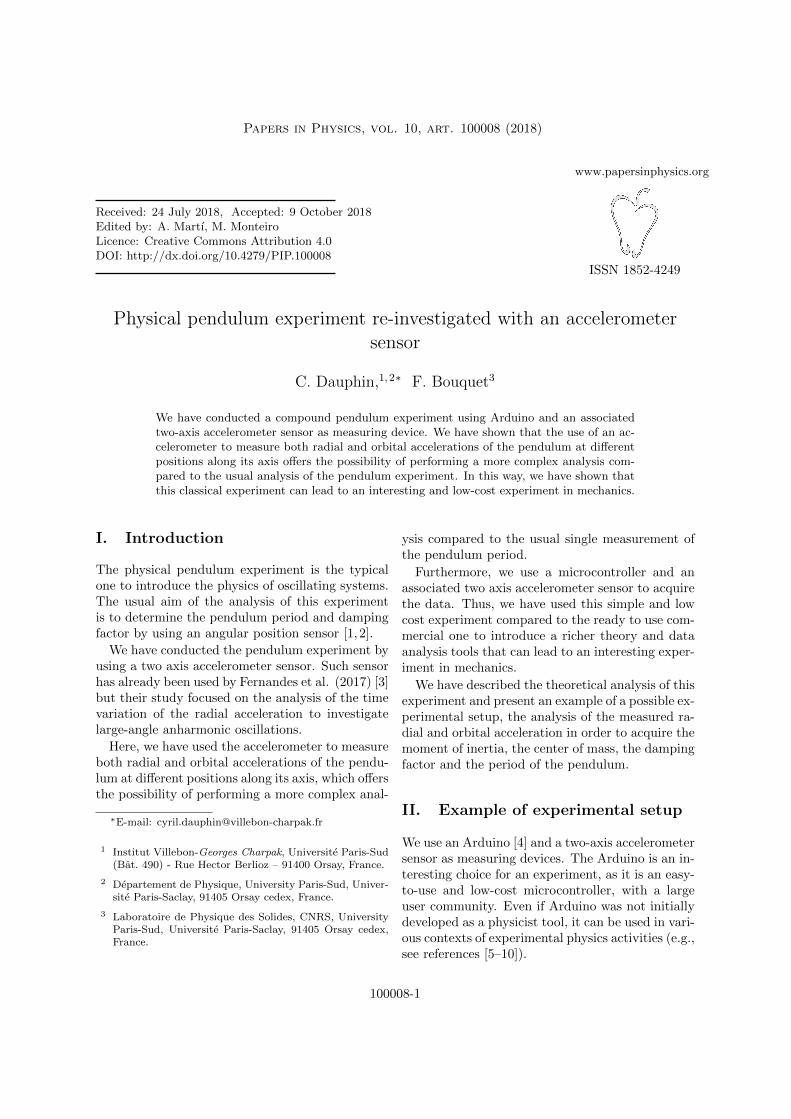
Figure 1: (a) An example of an experimental setup.(b) An accelerometer sensor attached to the centerlineof the pendulum, with one of its axes parallel to thecenterline.

The experimental setup that we used here isshown in Fig. 1(a). The accelerometer sensor isa microelectromechanical inertial sensor which isprecisely calibrated by using the values +g, 0g and−g for each axis with g = 9.8 m s−2.

The pendulum used in this experiment is com-posed of a bar on which masses can be attached todifferent positions. The accelerometer is attachedto the bar and positioned in such a way that one ofits measurement axes lies parallel to the bar (Fig.1(b)). Special care should be taken so that thewires connecting the accelerometer to the board areflexible enough in order not to damp the pendulum.

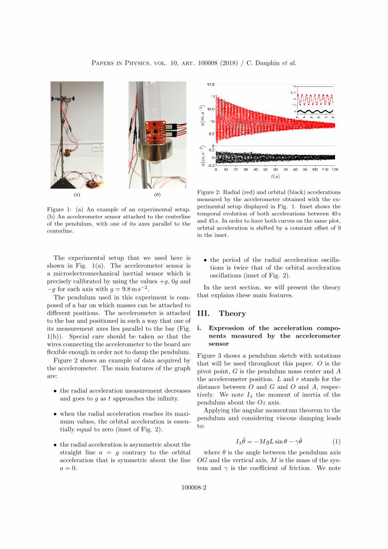
Figure 2 shows an example of data acquired bythe accelerometer. The main features of the graphare:

• the radial acceleration measurement decreasesand goes to g as t approaches the infinity.

• when the radial acceleration reaches its maxi-mum values, the orbital acceleration is essen-tially equal to zero (inset of Fig. 2).

• the radial acceleration is asymmetric about thestraight line a = g contrary to the orbitalacceleration that is symmetric about the linea = 0.

Figure 2: Radial (red) and orbital (black) accelerationsmeasured by the accelerometer obtained with the ex-perimental setup displayed in Fig. 1. Inset shows thetemporal evolution of both accelerations between 40 sand 45 s. In order to have both curves on the same plot,orbital acceleration is shifted by a constant offset of 9in the inset.

• the period of the radial acceleration oscilla-tions is twice that of the orbital accelerationoscillations (inset of Fig. 2).

In the next section, we will present the theorythat explains these main features.

III. Theory

i. Expression of the acceleration compo-nents measured by the accelerometersensor

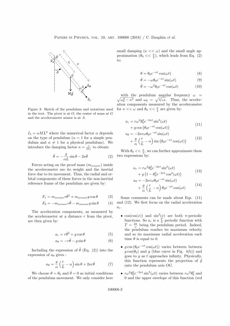
Figure 3 shows a pendulum sketch with notationsthat will be used throughout this paper. O is thepivot point, G is the pendulum mass center and Athe accelerometer position. L and r stands for thedistance between O and G and O and A, respec-tively. We note Iλ the moment of inertia of thependulum about the Oz axis.

Applying the angular momentum theorem to thependulum and considering viscous damping leadsto:

Iλθ = −MgL sin θ − γθ (1)

where θ is the angle between the pendulum axisOG and the vertical axis, M is the mass of the sys-tem and γ is the coefficient of friction. We note

100008-2


Figure 3: Sketch of the pendulum and notations usedin the text. The pivot is at O, the center of mass at Gand the accelerometer sensor is at A.

Iλ = αML2 where the numerical factor α dependson the type of pendulum (α = 1 for a simple pen-dulum and α 6= 1 for a physical pendulum). Weintroduce the damping factor κ = γ

2Iλto obtain:

θ = − g

αLsin θ − 2κθ (2)

Forces acting on the proof mass (msensor) insidethe accelerometer are its weight and the inertialforce due to its movement. Thus, the radial and or-bital components of these forces in the non-inertialreference frame of the pendulum are given by:

Fr = msensorrθ2 +msensorg cos θ (3)

Fθ = −msensorrθ −msensorg sin θ (4)

The acceleration components, as measured bythe accelerometer at a distance r from the pivot,are then given by:

ar = rθ2 + g cos θ (5)

aθ = −rθ − g sin θ (6)

Including the expression of θ (Eq. (2)) into theexpression of aθ gives :

aθ =g

α

( rL− α

)sin θ + 2κrθ (7)

We choose θ = θ0 and θ = 0 as initial conditionsof the pendulum movement. We only consider here

small damping (κ << ω) and the small angle ap-proximation (θ0 <<

π2 ), which leads from Eq. (2)

to:

θ = θ0e−κt cos(ωt) (8)

θ = −ωθ0e−κt sin(ωt) (9)

θ = −ω2θ0e−κt cos(ωt) (10)

with the pendulum angular frequency ω =√ω20 − κ2 and ω0 =

√g/αL. Thus, the acceler-

ation components measured by the accelerometerfor κ << ω and θ0 <<

π2 are given by:

ar = rω2θ20e−2κt sin2(ωt)

+ g cos(θ0e

−κt cos(ωt)) (11)

aθ = −2κrωθ0e−κt sin(ωt)

+g

α

( rL− α

)sin(θ0e


With θ0 <<π2 , we can further approximate these

two expressions by:

ar = rω2θ20e−2κt sin2(ωt)

+ g(1− θ20e−2κt cos2(ωt)

) (13)

aθ = −2κrωθ0e−κt sin(ωt)

+g

α

( rL− α

)θ0e

−κt cos(ωt)(14)

Some comments can be made about Eqs. (11)and (12). We first focus on the radial accelerationar.

• cos(cos(x)) and sin2(x) are both π-periodicfunctions. So ar is a T

2 periodic function withT = 2π

ω being the pendulum period. Indeed,the pendulum reaches its maximum velocityand so its maximum radial acceleration eachtime θ is equal to 0.

• g cos (θ0e−κt cos(ωt)) varies between between

g cos(θ0) and g (blue curve in Fig. 4(b)) andgoes to g as t approaches infinity. Physically,this function represents the projection of ~gonto the pendulum axis OG.

• rω2θ20e−2κt sin2(ωt) varies between rω2θ20 and

0 and the upper envelope of this function (red

100008-3


0 102 4 6 8 12 14 16

10

9.4

9.6

9.8

10.2

10.4

10.6

10.8

0 102 4 6 8 12 14 16

10

9.4

9.6

9.8

10.2

10.4

10.6

10.8

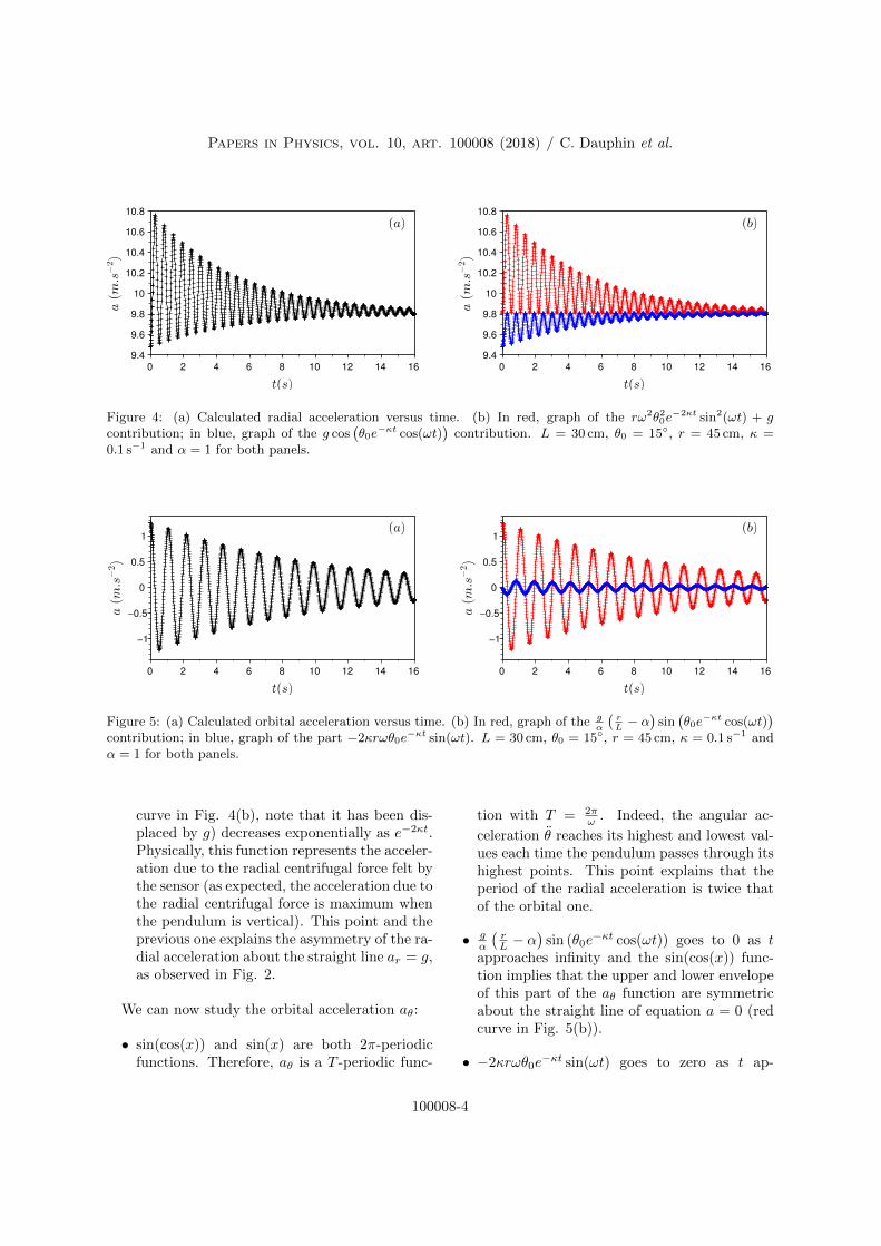
Figure 4: (a) Calculated radial acceleration versus time. (b) In red, graph of the rω2θ20e−2κt sin2(ωt) + g

contribution; in blue, graph of the g cos(θ0e

−κt cos(ωt))

contribution. L = 30 cm, θ0 = 15◦, r = 45 cm, κ =0.1 s−1 and α = 1 for both panels.

0 102 4 6 8 12 14 16

0

−1

1

−0.5

0.5

0 102 4 6 8 12 14 16

0

−1

1

−0.5

0.5

Figure 5: (a) Calculated orbital acceleration versus time. (b) In red, graph of the gα

(rL− α

)sin

(θ0e

−κt cos(ωt))

contribution; in blue, graph of the part −2κrωθ0e−κt sin(ωt). L = 30 cm, θ0 = 15◦, r = 45 cm, κ = 0.1 s−1 and

α = 1 for both panels.

curve in Fig. 4(b), note that it has been dis-placed by g) decreases exponentially as e−2κt.Physically, this function represents the acceler-ation due to the radial centrifugal force felt bythe sensor (as expected, the acceleration due tothe radial centrifugal force is maximum whenthe pendulum is vertical). This point and theprevious one explains the asymmetry of the ra-dial acceleration about the straight line ar = g,as observed in Fig. 2.

We can now study the orbital acceleration aθ:

• sin(cos(x)) and sin(x) are both 2π-periodicfunctions. Therefore, aθ is a T -periodic func-

tion with T = 2πω . Indeed, the angular ac-

celeration θ reaches its highest and lowest val-ues each time the pendulum passes through itshighest points. This point explains that theperiod of the radial acceleration is twice thatof the orbital one.

• gα

(rL − α

)sin (θ0e

−κt cos(ωt)) goes to 0 as tapproaches infinity and the sin(cos(x)) func-tion implies that the upper and lower envelopeof this part of the aθ function are symmetricabout the straight line of equation a = 0 (redcurve in Fig. 5(b)).

• −2κrωθ0e−κt sin(ωt) goes to zero as t ap-

100008-4


Figure 6: Radial (red) and orbital (black) accelerationsobtained from Eqs. (11) and (12) with θ0 = 20◦, L =30 cm, r = 34 cm, α = 1.2 and κ = 0.01 s−1. Insetshows the temporal evolution of radial (red) and orbital(black) accelerations between 40 s and 45 s. In order tohave both curves on the same plot, orbital accelerationis shifted by a constant offset of 9 in the inset.

proaches infinity. The upper and lower en-velopes of this part of the aθ function are sym-metric about the straight line aθ = 0 (bluecurve in Fig. 5(b)) and decrease exponentiallyas e−κt.

Figure 6 displays the radial (red) and orbital(black) accelerations obtained from Eqs. (11) and(12). We can see that the main features inferredfrom the data (Fig. 2) are well reproduced.

ii. Experimentally accessible quantities

The parameters describing the pendulum and itsmotion can be derived from the measurements ofar and aθ.

• ar(t = 0) = ar,min = g cos θ0. Thus, the mea-sured value of ar at t = 0 leads to the value ofθ0.

• A fit to the measured ar upper envelope withan exponential function allows us to determinethe damping factor κ of the pendulum fromEqs. (11) and (12). While, for small deflectionangles θ, see Eqs. (13) and (14), exponentialfit of any envelope of measured ar or aθ allowsus to determine the damping factor.

• The sensor position OA can be measured withgreat accuracy. Thus, the position of the pen-dulum center of mass and moment of inertiaare the two quantities which are difficult todetermine experimentally. Here, we use the fitof the temporal evolution of ar and aθ to de-termine the product αL.

iii. Impact of α and r on the measured ra-dial and orbital accelerations

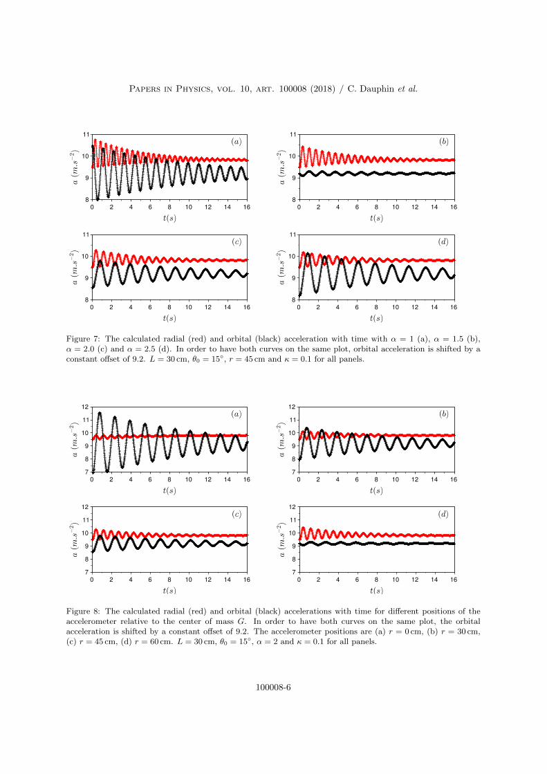
Figure 7 displays the evolution of the radial andorbital accelerations with time for different valuesof the moment of inertia (from α = 1 (Panel (a)) toα = 2.5 (Panel (d))). At the difference of the radialacceleration, we can see that the orbital accelera-tion depends strongly on α. Indeed, aθ expressionat t = 0 leads to aθ(t = 0) =

(rαL − 1

)g sin θ0,

which is an inverse function of α. We can also notethat aθ(t = 0) < 0 if α > r

L and aθ(t = 0) > 0 ifα < r

L . Thus, value of aθ at t = 0 gives informationon the α value.

Figure 8 shows the evolution of the radial andorbital accelerations with time for different valuesof r. The distance OA increases from Panel (a)to Panel (d). As expected, the amplitude of theradial acceleration increases with larger OA valuesas the centrifugal force acting on the proof massincreases and the amplitude of the orbital acceler-ation decreases with larger OA values as the rateof variation of θ decreases with this distance.

In particular, acceleration components measuredby the accelerometer attached to the position of thepoint O are given by:

ar = g cos(θ0e

−κt cos(ωt))

(15)

aθ = −g sin(θ0e

−κt cos(ωt))

(16)

In this case, the only force acting on the mass insidethe accelerometer is its weight and the expressionsof the acceleration do not depend on α. Accelerom-eter sensor is used in this case as an angular posi-tion sensor.

We also note that the acceleration componentsmeasured by the accelerometer attached to the po-sition r = Lα are given by:

100008-5


0 102 4 6 8 12 14 16

10

8

9

11

0 102 4 6 8 12 14 16

10

8

9

11

0 102 4 6 8 12 14 16

10

8

9

11

0 102 4 6 8 12 14 16

10

8

9

11

Figure 7: The calculated radial (red) and orbital (black) acceleration with time with α = 1 (a), α = 1.5 (b),α = 2.0 (c) and α = 2.5 (d). In order to have both curves on the same plot, orbital acceleration is shifted by aconstant offset of 9.2. L = 30 cm, θ0 = 15◦, r = 45 cm and κ = 0.1 for all panels.

0 102 4 6 8 12 14 16

10

8

12

7

9

11

0 102 4 6 8 12 14 16

10

8

12

7

9

11

0 102 4 6 8 12 14 16

10

8

12

7

9

11

0 102 4 6 8 12 14 16

10

8

12

7

9

11

Figure 8: The calculated radial (red) and orbital (black) accelerations with time for different positions of theaccelerometer relative to the center of mass G. In order to have both curves on the same plot, the orbitalacceleration is shifted by a constant offset of 9.2. The accelerometer positions are (a) r = 0 cm, (b) r = 30 cm,(c) r = 45 cm, (d) r = 60 cm. L = 30 cm, θ0 = 15◦, α = 2 and κ = 0.1 for all panels.

100008-6


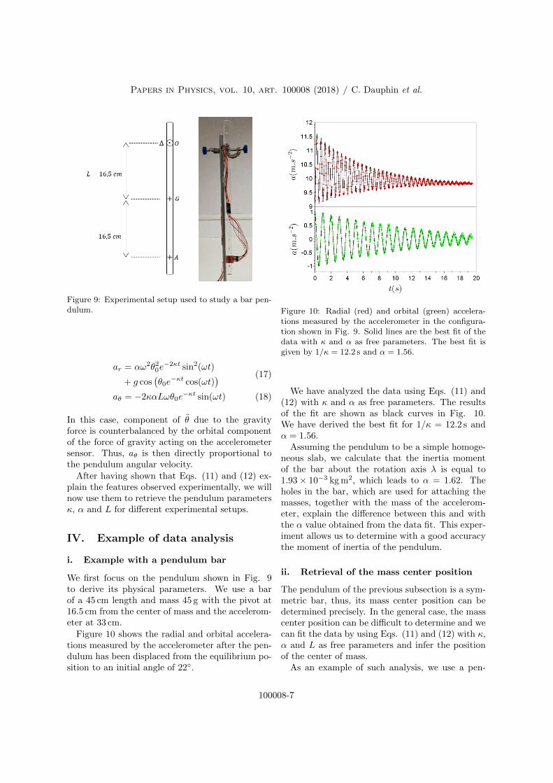
Figure 9: Experimental setup used to study a bar pen-dulum.

ar = αω2θ20e−2κt sin2(ωt)

+ g cos(θ0e


aθ = −2καLωθ0e−κt sin(ωt) (18)

In this case, component of θ due to the gravityforce is counterbalanced by the orbital componentof the force of gravity acting on the accelerometersensor. Thus, aθ is then directly proportional tothe pendulum angular velocity.

After having shown that Eqs. (11) and (12) ex-plain the features observed experimentally, we willnow use them to retrieve the pendulum parametersκ, α and L for different experimental setups.

IV. Example of data analysis

i. Example with a pendulum bar

We first focus on the pendulum shown in Fig. 9to derive its physical parameters. We use a barof a 45 cm length and mass 45 g with the pivot at16.5 cm from the center of mass and the accelerom-eter at 33 cm.

Figure 10 shows the radial and orbital accelera-tions measured by the accelerometer after the pen-dulum has been displaced from the equilibrium po-sition to an initial angle of 22◦.

Figure 10: Radial (red) and orbital (green) accelera-tions measured by the accelerometer in the configura-tion shown in Fig. 9. Solid lines are the best fit of thedata with κ and α as free parameters. The best fit isgiven by 1/κ = 12.2 s and α = 1.56.

We have analyzed the data using Eqs. (11) and(12) with κ and α as free parameters. The resultsof the fit are shown as black curves in Fig. 10.We have derived the best fit for 1/κ = 12.2 s andα = 1.56.

Assuming the pendulum to be a simple homoge-neous slab, we calculate that the inertia momentof the bar about the rotation axis λ is equal to1.93× 10−3 kg m2, which leads to α = 1.62. Theholes in the bar, which are used for attaching themasses, together with the mass of the accelerom-eter, explain the difference between this and withthe α value obtained from the data fit. This exper-iment allows us to determine with a good accuracythe moment of inertia of the pendulum.

ii. Retrieval of the mass center position

The pendulum of the previous subsection is a sym-metric bar, thus, its mass center position can bedetermined precisely. In the general case, the masscenter position can be difficult to determine and wecan fit the data by using Eqs. (11) and (12) with κ,α and L as free parameters and infer the positionof the center of mass.

As an example of such analysis, we use a pen-

100008-7


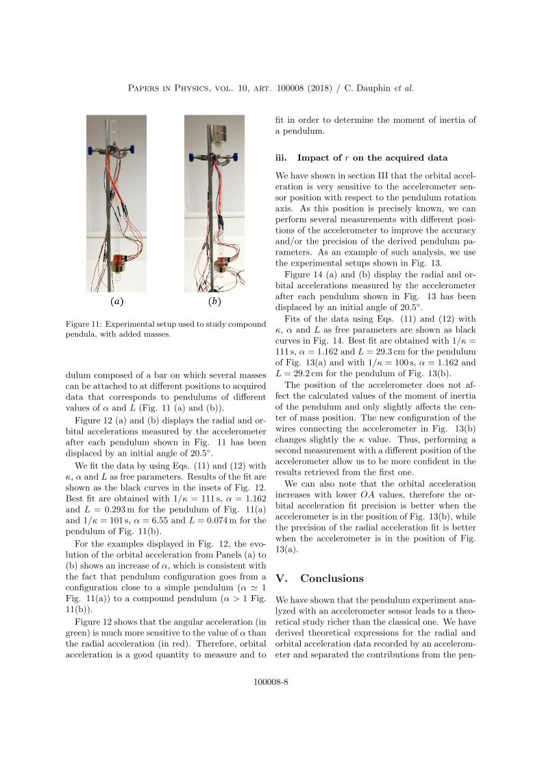
Figure 11: Experimental setup used to study compoundpendula, with added masses.

dulum composed of a bar on which several massescan be attached to at different positions to acquireddata that corresponds to pendulums of differentvalues of α and L (Fig. 11 (a) and (b)).

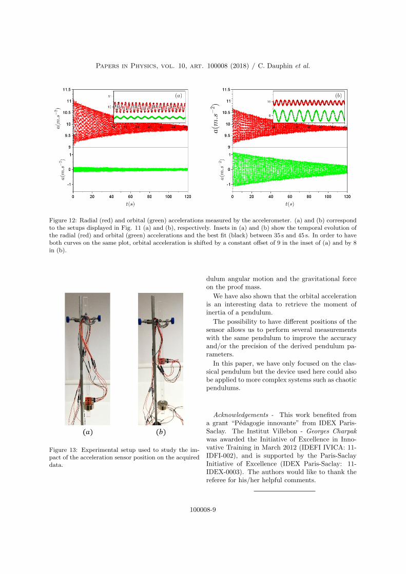
Figure 12 (a) and (b) displays the radial and or-bital accelerations measured by the accelerometerafter each pendulum shown in Fig. 11 has beendisplaced by an initial angle of 20.5◦.

We fit the data by using Eqs. (11) and (12) withκ, α and L as free parameters. Results of the fit areshown as the black curves in the insets of Fig. 12.Best fit are obtained with 1/κ = 111 s, α = 1.162and L = 0.293 m for the pendulum of Fig. 11(a)and 1/κ = 101 s, α = 6.55 and L = 0.074 m for thependulum of Fig. 11(b).

For the examples displayed in Fig. 12, the evo-lution of the orbital acceleration from Panels (a) to(b) shows an increase of α, which is consistent withthe fact that pendulum configuration goes from aconfiguration close to a simple pendulum (α ' 1Fig. 11(a)) to a compound pendulum (α > 1 Fig.11(b)).

Figure 12 shows that the angular acceleration (ingreen) is much more sensitive to the value of α thanthe radial acceleration (in red). Therefore, orbitalacceleration is a good quantity to measure and to

fit in order to determine the moment of inertia ofa pendulum.

iii. Impact of r on the acquired data

We have shown in section III that the orbital accel-eration is very sensitive to the accelerometer sen-sor position with respect to the pendulum rotationaxis. As this position is precisely known, we canperform several measurements with different posi-tions of the accelerometer to improve the accuracyand/or the precision of the derived pendulum pa-rameters. As an example of such analysis, we usethe experimental setups shown in Fig. 13.

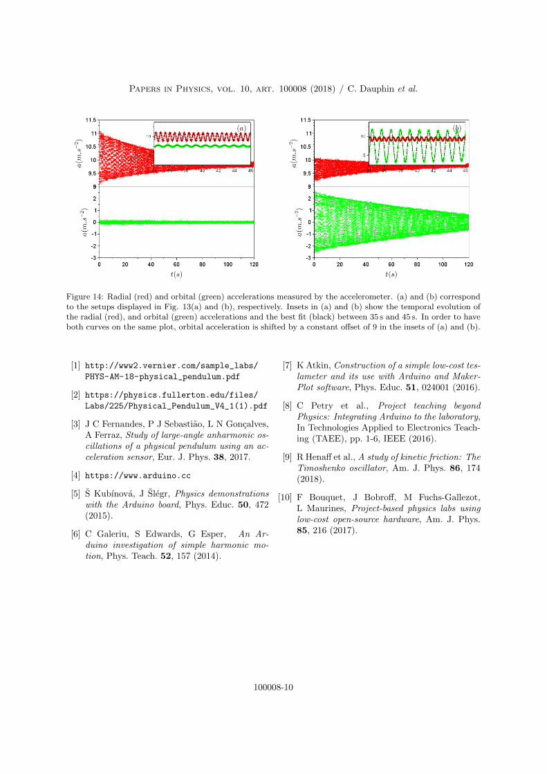
Figure 14 (a) and (b) display the radial and or-bital accelerations measured by the accelerometerafter each pendulum shown in Fig. 13 has beendisplaced by an initial angle of 20.5◦.

Fits of the data using Eqs. (11) and (12) withκ, α and L as free parameters are shown as blackcurves in Fig. 14. Best fit are obtained with 1/κ =111 s, α = 1.162 and L = 29.3 cm for the pendulumof Fig. 13(a) and with 1/κ = 100 s, α = 1.162 andL = 29.2 cm for the pendulum of Fig. 13(b).

The position of the accelerometer does not af-fect the calculated values of the moment of inertiaof the pendulum and only slightly affects the cen-ter of mass position. The new configuration of thewires connecting the accelerometer in Fig. 13(b)changes slightly the κ value. Thus, performing asecond measurement with a different position of theaccelerometer allow us to be more confident in theresults retrieved from the first one.

We can also note that the orbital accelerationincreases with lower OA values, therefore the or-bital acceleration fit precision is better when theaccelerometer is in the position of Fig. 13(b), whilethe precision of the radial acceleration fit is betterwhen the accelerometer is in the position of Fig.13(a).

V. Conclusions

We have shown that the pendulum experiment ana-lyzed with an accelerometer sensor leads to a theo-retical study richer than the classical one. We havederived theoretical expressions for the radial andorbital acceleration data recorded by an accelerom-eter and separated the contributions from the pen-

100008-8


Figure 12: Radial (red) and orbital (green) accelerations measured by the accelerometer. (a) and (b) correspondto the setups displayed in Fig. 11 (a) and (b), respectively. Insets in (a) and (b) show the temporal evolution ofthe radial (red) and orbital (green) accelerations and the best fit (black) between 35 s and 45 s. In order to haveboth curves on the same plot, orbital acceleration is shifted by a constant offset of 9 in the inset of (a) and by 8in (b).

Figure 13: Experimental setup used to study the im-pact of the acceleration sensor position on the acquireddata.

dulum angular motion and the gravitational forceon the proof mass.

We have also shown that the orbital accelerationis an interesting data to retrieve the moment ofinertia of a pendulum.

The possibility to have different positions of thesensor allows us to perform several measurementswith the same pendulum to improve the accuracyand/or the precision of the derived pendulum pa-rameters.

In this paper, we have only focused on the clas-sical pendulum but the device used here could alsobe applied to more complex systems such as chaoticpendulums.

Acknowledgements - This work benefited froma grant “Pedagogie innovante” from IDEX Paris-Saclay. The Institut Villebon - Georges Charpakwas awarded the Initiative of Excellence in Inno-vative Training in March 2012 (IDEFI IVICA: 11-IDFI-002), and is supported by the Paris-SaclayInitiative of Excellence (IDEX Paris-Saclay: 11-IDEX-0003). The authors would like to thank thereferee for his/her helpful comments.

100008-9


Figure 14: Radial (red) and orbital (green) accelerations measured by the accelerometer. (a) and (b) correspondto the setups displayed in Fig. 13(a) and (b), respectively. Insets in (a) and (b) show the temporal evolution ofthe radial (red), and orbital (green) accelerations and the best fit (black) between 35 s and 45 s. In order to haveboth curves on the same plot, orbital acceleration is shifted by a constant offset of 9 in the insets of (a) and (b).

[1] http://www2.vernier.com/sample_labs/

PHYS-AM-18-physical_pendulum.pdf

[2] https://physics.fullerton.edu/files/

Labs/225/Physical_Pendulum_V4_1(1).pdf

[3] J C Fernandes, P J Sebastiao, L N Goncalves,A Ferraz, Study of large-angle anharmonic os-cillations of a physical pendulum using an ac-celeration sensor, Eur. J. Phys. 38, 2017.

[4] https://www.arduino.cc

[5] S Kubınova, J Slegr, Physics demonstrationswith the Arduino board, Phys. Educ. 50, 472(2015).

[6] C Galeriu, S Edwards, G Esper, An Ar-duino investigation of simple harmonic mo-tion, Phys. Teach. 52, 157 (2014).

[7] K Atkin, Construction of a simple low-cost tes-lameter and its use with Arduino and Maker-Plot software, Phys. Educ. 51, 024001 (2016).

[8] C Petry et al., Project teaching beyondPhysics: Integrating Arduino to the laboratory,In Technologies Applied to Electronics Teach-ing (TAEE), pp. 1-6, IEEE (2016).

[9] R Henaff et al., A study of kinetic friction: TheTimoshenko oscillator, Am. J. Phys. 86, 174(2018).

[10] F Bouquet, J Bobroff, M Fuchs-Gallezot,L Maurines, Project-based physics labs usinglow-cost open-source hardware, Am. J. Phys.85, 216 (2017).

100008-10

physical pendulum experiment re-investigated with an

Documents