physical drivers of climate change
TRANSCRIPT

University of Nebraska - LincolnDigitalCommons@University of Nebraska - LincolnPublications, Agencies and Staff of the U.S.Department of Commerce U.S. Department of Commerce
2017
Physical drivers of climate changeDavid FaheyNOAA Earth System Research Lab
Sarah DohertyUniversity of Washington
Kathleen A. HibbardNASA Headquarters, [email protected]
Anastasia RomanouColumbia University, [email protected]
Patrick TaylorNASA Langley Research Center
Follow this and additional works at: http://digitalcommons.unl.edu/usdeptcommercepub
This Article is brought to you for free and open access by the U.S. Department of Commerce at DigitalCommons@University of Nebraska - Lincoln. Ithas been accepted for inclusion in Publications, Agencies and Staff of the U.S. Department of Commerce by an authorized administrator ofDigitalCommons@University of Nebraska - Lincoln.
Fahey, David; Doherty, Sarah; Hibbard, Kathleen A.; Romanou, Anastasia; and Taylor, Patrick, "Physical drivers of climate change"(2017). Publications, Agencies and Staff of the U.S. Department of Commerce. 591.http://digitalcommons.unl.edu/usdeptcommercepub/591

Physical drivers of climate change
David Fahey, NOAA Earth System Research Lab
Sarah Doherty, University of Washington
Kathleen Hibbard, NASA Headquarters
Anastasia Romanou, Columbia University
Patrick Taylor, NASA Langley Research Center
Citation: In: Climate Science Special Report: A Sustained Assessment Activity of the U.S. Global Change
Research Program [Wuebbles, D.J., D.W. Fahey, K.A. Hibbard, D.J. Dokken, B.C. Stewart, and T.K. Maycock
(eds.)]. U.S. Global Change Research Program, Washington, DC, USA (2017), pp. 98-159.
Comments: U.S. Government work
Abstract
1. Human activities continue to significantly affect Earth’s climate by altering factors that change its radiative
balance. These factors, known as radiative forcings, include changes in greenhouse gases, small airborne
particles (aerosols), and the reflectivity of the Earth’s surface. In the industrial era, human activities have
been, and are increasingly, the dominant cause of climate warming. The increase in radiative forcing due to
these activities has far exceeded the relatively small net increase due to natural factors, which include
changes in energy from the sun and the cooling effect of volcanic eruptions. (Very high confidence)
2. Aerosols caused by human activity play a profound and complex role in the climate system through
radiative effects in the atmosphere and on snow and ice surfaces and through effects on cloud formation and
properties. The combined forcing of aerosol–radiation and aerosol– cloud interactions is negative (cooling)
over the industrial era (high confidence), offsetting a substantial part of greenhouse gas forcing, which is
currently the predominant human contribution. The magnitude of this offset, globally averaged, has declined
in recent decades, despite increasing trends in aerosol emissions or abundances in some regions (medium to
high confidence)
3. The interconnected Earth–atmosphere–ocean system includes a number of positive and negative feedback
processes that can either strengthen (positive feedback) or weaken (negative feedback) the system’s
responses to human and natural influences. These feedbacks operate on a range of timescales from very short
(essentially instantaneous) to very long (centuries). Global warming by net radiative forcing over the
industrial era includes a substantial amplification from these feedbacks (approximately a factor of three)
(high confidence).
While there are large uncertainties associated with some of these feedbacks, the net feedback effect over the
industrial era has been positive (amplifying warming) and will continue to be positive in coming decades
(Very high confidence).

CSSR 5OD: FINAL CLEARANCE Chapter 2
Subject to Final Copyedit 28 June 201798
2. Physical Drivers of Climate Change 1
Key Findings 2
1. Human activities continue to significantly affect Earth’s climate by altering factors that 3 change its radiative balance. These factors, known as radiative forcings, include changes in 4 greenhouse gases, small airborne particles (aerosols), and the reflectivity of the Earth’s 5 surface. In the industrial era, human activities have been, and are increasingly, the dominant 6 cause of climate warming. The increase in radiative forcing due to these activities has far 7 exceeded the relatively small net increase due to natural factors, which include changes in 8 energy from the sun and the cooling effect of volcanic eruptions. (Very high confidence) 9
2. Aerosols caused by human activity play a profound and complex role in the climate system 10 through radiative effects in the atmosphere and on snow and ice surfaces and through effects 11 on cloud formation and properties. The combined forcing of aerosol–radiation and aerosol–12 cloud interactions is negative (cooling) over the industrial era (high confidence), offsetting a 13 substantial part of greenhouse gas forcing, which is currently the predominant human 14 contribution. The magnitude of this offset, globally averaged, has declined in recent decades, 15 despite increasing trends in aerosol emissions or abundances in some regions (medium to 16 high confidence) 17
3. The interconnected Earth–atmosphere–ocean system includes a number of positive and 18 negative feedback processes that can either strengthen (positive feedback) or weaken 19 (negative feedback) the system’s responses to human and natural influences. These feedbacks 20 operate on a range of timescales from very short (essentially instantaneous) to very long 21 (centuries). Global warming by net radiative forcing over the industrial era includes a 22 substantial amplification from these feedbacks (approximately a factor of three) (high 23 confidence). While there are large uncertainties associated with some of these feedbacks, the 24 net feedback effect over the industrial era has been positive (amplifying warming) and will 25 continue to be positive in coming decades (Very high confidence). 26
2.0 Introduction 27
Earth’s climate is undergoing substantial change due to anthropogenic activities (Ch. 1: Our 28 Globally Changing Climate). Understanding the causes of past and present climate change and 29 confidence in future projected changes depend directly on our ability to understand and model 30 the physical drivers of climate change (Clark et al. 2016). Our understanding is challenged by the 31 complexity and interconnectedness of the components of the climate system (that is, the 32 atmosphere, land, ocean, and cryosphere). This chapter lays out the foundation of climate change 33 by describing its physical drivers, which are primarily associated with atmospheric composition 34 (gases and aerosols) and cloud effects. We describe the principle radiative forcings and the 35 variety of feedback responses which serve to amplify these forcings. 36

CSSR 50D: FINAL CLEARANCE Chapter 2
1 2.1 Earth's Energy Balance and the Greenhouse Effect
2 The temperature of the Earth system is detennined by the amounts of incoming (5hort-
3 wavelength) and outgoing (bodl short- and long-wavelengdl) radiation . In die modem era ,
4 radiative fluxes are well-constrained by satellite measurements (Figure 2.1) . About a third
5 (29 .4%) of incoming. short-wavelengdl energy from the sun is reflected back to space and the
6 remainder is absorbed by the Eardl system. The fraction of sunlight scattered back to space is 7 detennilled by the reflectivity (albedo) of clouds, land surfaces (including snow and ice) , oceans,
8 and particles in dIe atmosphere. TIle amount and albedo of clouds, snow cover, and ice cover are
9 particularly strong detemunants of dIe amount of sunlight reflected back to space because their
10 albedos are much higher than dlat of land and oceans.
11 In addition to reflected sunlight , Earth loses energy through infrared (long-wavelength) radiation
12 from dIe surface and atmosphere. Greenhouse gases (GHGs) in the atmosphere absorb most of
13 this radiation, leading to a wanning of the surface and atmosphere. Figure 2.1 illustrates the
14 importance of greenhouse gases in the energy balance of the Earth system. The naturally 15 occurring GHGs in Earth's atmosphere-principally water vapor and carbon dioxide-keep the 16 near-surface air temperature about 60°F (33°C) wanner than it would be in dleir absence,
17 assuming albedo is held constant (Lacis et al. 2010). Geodlermal heat from Earth 's interior ,
18 direct heating from energy production, and frictional heating through tidal flows also contribute
19 to dIe amount of energy available for heating dIe Earth's surface and atmosphere , but dleir total
20 contribution is an extremely small fraction « 0.1 %) of that due to net solar (shortwave) and 21 infrared (longwave) radiation (e .g. , see Davies and Davies 2010; FlaImer 2009; Munk and
22 Wunsch 1998, where these forcings are qUaIltified).
23 [INSERT FIGURE 2.1 HERE]
24 Thus, Earth's equilibrium temperature in dIe modem era is controlled by a short list of factors:
25 incoming sunlight , absorbed aIld reflected sunlight , emitted infrared radiation, and infrared 26 radiation absorbed and re-emitted in the atmosphere , primarily by GHGs. ChaIlges in these
27 factors affect Earth's radiative balaIlce aIld therefore its climate, including but not limited to the
28 average , near-surface air temperature. Andrropogenic activities have changed Earth's radiative
29 balance and its albedo by adding GHGs, particles (aerosols), and aircraft contrails to dIe 30 atmosphere , aIld tlrrough laIld-use changes. ChaIlges in the radiative balaIlce (or forcings)
31 produce changes in temperature , precipitation, and other climate variables drrough a complex set
32 of physical processes, maIlY of which are coupled (Figllfe 2.2) . These changes, in tum, trigger 33 feedback processes which can further amplify aIHi/or dampen the changes in radiative balaIlce
34 (Sections 2.5 and 2 .6) .
35 In the following sections, the principal components of dIe framework shown in Figure 2.2 are
36 described. Climate models are structllfed to represent these processes; climate models and their
37 components and associated uncertainties, are discussed in more detail in Chapter 4: Projections .
Subject to Final Copyedit 99 28 June 2017

CSSR 5OD: FINAL CLEARANCE Chapter 2
Subject to Final Copyedit 28 June 2017100
[INSERT FIGURE 2.2 HERE] 1
The processes and feedbacks connecting changes in Earth’s radiative balance to a climate 2 response (Figure 2.2) operate on a large range of timescales. Reaching an equilibrium 3 temperature distribution in response to anthropogenic activities takes decades or longer because 4 some components of the Earth system—in particular the oceans and cryosphere—are slow to 5 respond due to their large thermal masses and the long timescale of circulation between the 6 ocean surface and the deep ocean. Of the substantial energy gained in the combined ocean–7 atmosphere system over the previous four decades, over 90% of it has gone into ocean warming 8 (Rhein et al. 2013; see Box 3.1 Fig 1). Even at equilibrium, internal variability in Earth’s climate 9 system causes limited annual- to decadal-scale variations in regional temperatures and other 10 climate parameters that do not contribute to long-term trends. For example, it is likely that 11 natural variability has contributed between −0.18°F (−0.1°C) and 0.18°F (0.1°C) to changes in 12 surface temperatures from 1951 to 2010; by comparison, anthropogenic GHGs have likely 13 contributed between 0.9°F (0.5°C) and 2.3°F (1.3°C) to observed surface warming over this 14 same period (Bindoff et al. 2013). Due to these longer timescale responses and natural 15 variability, changes in Earth’s radiative balance are not realized immediately as changes in 16 climate, and even in equilibrium there will always be variability around mean conditions. 17
2.2 Radiative Forcing (RF) and Effective Radiative Forcing (ERF) 18
Radiative forcing (RF) is widely used to quantify a radiative imbalance in Earth’s atmosphere 19 resulting from either natural changes or anthropogenic activities over the industrial era. It is 20 expressed as a change in net radiative flux (W/m2) either at the tropopause or top of the 21 atmosphere (Myhre et al. 2013), with the latter nominally defined at 20 km altitude to optimize 22 observation/model comparisons (Loeb et al. 2002). The instantaneous RF is defined as the 23 immediate change in net radiative flux following a change in a climate driver. RF can also be 24 calculated after allowing different types of system response: for example, after allowing 25 stratospheric temperatures to adjust, after allowing both stratospheric and surface temperature to 26 adjust, or after allowing temperatures to adjust everywhere (the equilibrium RF) (Figure 8.1 of 27 Myhre et al. 2013). 28
In this report, we follow the Intergovernmental Panel on Climate Change (IPCC) 29 recommendation that the RF caused by a forcing agent be evaluated as the net radiative flux 30 change at the tropopause after stratospheric temperatures have adjusted to a new radiative 31 equilibrium while assuming all other variables (for example, temperatures and cloud cover) are 32 held fixed (Box 8.1 of Myhre et al. 2013). A change that results in a net increase in the 33 downward flux (shortwave plus longwave) constitutes a positive RF, normally resulting in a 34 warming of the surface and/or atmosphere and potential changes in other climate parameters. 35 Conversely, a change that yields an increase in the net upward flux constitutes a negative RF, 36 leading to a cooling of the surface and/or atmosphere and potential changes in other climate 37 parameters. 38

CSSR 5OD: FINAL CLEARANCE Chapter 2
Subject to Final Copyedit 28 June 2017101
RF serves as a metric to compare present, past, or future perturbations to the climate system 1 (e.g., Boer and Yu 2003; Gillett et al. 2004; Matthews et al. 2004; Meehl et al. 2004; Jones et al. 2 2007; Mahajan et al. 2013; Shiogama et al. 2013). For clarity and consistency, RF calculations 3 require that a time period be defined over which the forcing occurs. Here, this period is the 4 industrial era, defined as beginning in 1750 and extending to 2011, unless otherwise noted. The 5 2011 end date is that adopted by the CMIP5 calculations, which are the basis of RF evaluations 6 by the IPCC (Myhre et al. 2013). 7
A refinement of the RF concept introduced in the latest IPCC assessment (IPCC 2013) is the use 8 of effective radiative forcing (ERF). ERF for a climate driver is defined as its RF plus rapid 9 adjustment(s) to that RF (Myhre et al. 2013). These rapid adjustments occur on timescales much 10 shorter than, for example, the response of ocean temperatures. For an important subset of climate 11 drivers, ERF is more reliably correlated with the climate response to the forcing than is RF; as 12 such, it is an increasingly used metric when discussing forcing. For atmospheric components, 13 ERF includes rapid adjustments due to direct warming of the troposphere, which produces 14 horizontal temperature variations, variations in the vertical lapse rate, and changes in clouds and 15 vegetation, and it includes the microphysical effects of aerosols on cloud lifetime. Rapid changes 16 in land surface properties (temperature, snow and ice cover, and vegetation) are also included. 17 Not included in ERF are climate responses driven by changes in sea surface temperatures or sea 18 ice cover. For forcing by aerosols in snow (Section 2.3.2), ERF includes the effects of direct 19 warming of the snowpack by particulate absorption (for example, snow-grain size changes). 20 Changes in all of these parameters in response to RF are quantified in terms of their impact on 21 radiative fluxes (for example, albedo) and included in the ERF. The largest differences between 22 RF and ERF occur for forcing by light-absorbing aerosols because of their influence on clouds 23 and snow (Section 2.3.2). For most non-aerosol climate drivers, the differences between RF and 24 ERF are small. 25
2.3 Drivers of Climate Change over the Industrial Era 26
Climate drivers of significance over the industrial era include both those associated with 27 anthropogenic activity and, to a lesser extent, those of natural origin. The only significant natural 28 climate drivers in the industrial era are changes in solar irradiance, volcanic eruptions, and the El 29 Niño–Southern Oscillation. Natural emissions and sinks of GHGs and tropospheric aerosols have 30 varied over the industrial era but have not contributed significantly to RF. The effects of cosmic 31 rays on cloud formation have been studied, but global radiative effects are not considered 32 significant (Krissansen-Totton and Davies 2013). There are other known drivers of natural origin 33 that operate on longer timescales (for example, changes in Earth’s orbit [Milankovitch cycles] 34 and changes in atmospheric CO2 via chemical weathering of rock). Anthropogenic drivers can be 35 divided into a number of categories, including well-mixed greenhouse gases (WMGHGs), short-36 lived climate forcers (SLCFs, which include methane, some hydrofluorocarbons [HFCs], ozone, 37 and aerosols), contrails, and changes in albedo (for example, land-use changes). Some 38

CSSR 5OD: FINAL CLEARANCE Chapter 2
Subject to Final Copyedit 28 June 2017102
WMGHGs are also considered SLCFs (for example, methane). Figures 2.3–2.7 summarize 1 features of the principal climate drivers in the industrial era. Each is described briefly in the 2 following. 3
[INSERT FIGURE 2.3 HERE] 4
2.3.1 Natural Drivers 5
SOLAR IRRADIANCE 6
Changes in solar irradiance directly impact the climate system because the irradiance is Earth's 7 primary energy source (Lean 1997). In the industrial era, the largest variations in total solar 8 irradiance follow an 11-year cycle (Frölich and Lean 2004; Gray et al. 2010). Direct solar 9 observations have been available since 1978 (Kopp 2014), though proxy indicators of solar 10 cycles are available back to the early 1600s (Kopp et al. 2016). Although these variations 11 amount to only 0.1% of the total solar output of about 1360 W/m2 (Kopp and Lean 2011), 12 relative variations in irradiance at specific wavelengths can be much larger (tens of percent). 13 Spectral variations in solar irradiance are highest at near-ultraviolet (UV) and shorter 14 wavelengths (Floyd et al. 2003), which are also the most important wavelengths for driving 15 changes in ozone (Ermolli et al. 2013; Bolduc et al. 2015). By affecting ozone concentrations, 16 variations in total and spectral solar irradiance induce discernible changes in atmospheric heating 17 and changes in circulation (Gray et al. 2010; Lockwood 2012; Seppälä et al. 2014). The 18 relationships between changes in irradiance and changes in atmospheric composition, heating, 19 and dynamics are such that changes in total solar irradiance are not directly correlated with the 20 resulting radiative flux changes (Ermolli et al. 2013; Xu and Powell 2013; Gao et al. 2015). 21
The IPCC estimate of the RF due to changes in total solar irradiance over the industrial era is 22 0.05 W/m2 (range: 0.0 to 0.10 W/m2) (Myhre et al. 2013). This forcing does not account for 23 radiative flux changes resulting from changes in ozone driven by changes in the spectral 24 irradiance. Understanding of the links between changes in spectral irradiance, ozone 25 concentrations, heating rates, and circulation changes has recently improved using, in particular, 26 satellite data starting in 2002 that provide solar spectral irradiance measurements through the UV 27 (Ermolli et al. 2013) along with a series of chemistry–climate modeling studies (Swartz et al. 28 2012; Chiodo et al. 2014; Dhomse et al. 2013; Ermolli et al. 2013; Bolduc et al. 2015). At the 29 regional scale, circulation changes driven by solar spectral irradiance variations may be 30 significant for some locations and seasons, but are poorly quantified (Lockwood 2012). Despite 31 remaining uncertainties, there is very high confidence that solar radiance-induced changes in RF 32 are small relative to RF from anthropogenic GHGs over the industrial era (Myhre et al. 2013) 33 (Figure 2.3). 34
35

CSSR 5OD: FINAL CLEARANCE Chapter 2
Subject to Final Copyedit 28 June 2017103
VOLCANOES 1
Most volcanic eruptions are minor events with the effects of emissions confined to the 2 troposphere and only lasting for weeks to months. In contrast, explosive volcanic eruptions inject 3 substantial amounts of sulfur dioxide (SO2) and ash into the stratosphere, which leads to 4 significant short-term climate effects (Myhre et al. 2013, and references therein). SO2 oxidizes to 5 form sulfuric acid (H2SO4) which condenses, forming new particles or adding mass to 6 preexisting particles, thereby substantially enhancing the attenuation of sunlight transmitted 7 through the stratosphere (that is, increasing aerosol optical depth). These aerosols increase the 8 Earth’s albedo by scattering sunlight back to space, creating a negative RF that cools the planet 9 (Andronova et al. 1999; Robock 2000). The RF persists for the lifetime of aerosol in the 10 stratosphere, which is a few years, far exceeding that in the troposphere (about a week). The 11 oceans respond to a negative volcanic RF through cooling and changes in ocean circulation 12 patterns that last for decades after major eruptions (for example, Mt. Tambora in 1815) 13 (Stenchikov et al. 2009; Otterå et al. 2010; Zanchettin et al. 2012; Zhang et al. 2013). In addition 14 to the direct RF, volcanic aerosol heats the stratosphere, altering circulation patterns, and 15 depletes ozone by enhancing surface reactions, which further changes heating and circulation. 16 The resulting impacts on advective heat transport can be larger than the temperature impacts of 17 the direct forcing (Robock 2000). Aerosol from both explosive and non-explosive eruptions also 18 affects the troposphere through changes in diffuse radiation and through aerosol–cloud 19 interactions. It has been proposed that major eruptions might “fertilize” the ocean with sufficient 20 iron to affect phyotoplankton production and, therefore, enhance the ocean carbon sink 21 (Langmann 2014). Volcanoes also emit CO2 and water vapor, although in small quantities 22 relative to other emissions. At present, conservative estimates of annual CO2 emissions from 23 volcanoes are less than 1% of CO2 emissions from all anthropogenic activities (Gerlach 2011). 24 The magnitude of volcanic effects on climate depend on the number and strengths of eruptions, 25 the latitude of injection and, for ocean temperature and circulation impacts, the timing of the 26 eruption relative to ocean temperature and circulation patterns (Zanchettin et al. 2012; Zhang et 27 al. 2013). 28
Volcanic eruptions represent the largest natural forcing within the industrial era. In the last 29 millennium, eruptions caused several multiyear, transient episodes of negative RF of up to 30 several W/m2 (Figure 2.6). The RF of the last major volcanic eruption, Mt. Pinatubo in 1991, 31 decayed to negligible values later in the 1990s, with the temperature signal lasting about twice as 32 long due to the effects of changes in ocean heat uptake (Stenchikov et al. 2009). A net volcanic 33 RF has been omitted from the drivers of climate change in the industrial era in Figure 2.3 34 because the value from multiple, episodic eruptions is negligible compared with the other climate 35 drivers. While future explosive volcanic eruptions have the potential to again alter Earth’s 36 climate for periods of several years, predictions of occurrence, intensity, and location remain 37 elusive. If a sufficient number of non-explosive eruptions occur over an extended time period in 38

CSSR 50D: FINAL CLEARANCE Chapter 2
1 the future . average changes in tropospheric composition or circulation could yield a significant
2 RF (Robock 2000) .
3 2.3.2 Anthropogenic Drivers
4 PRINCIPAL WELL-MIXED GREENHOUSE GASES (WMGHGs)
5 The principal WMGHGs are carbon dioxide (COJ , methane (CH4) . and nitrous oxide (NzO) . 6 With atmospheric lifetimes of a decade or more , these gases have modest-ta-small regional
7 variabilities and are circulated and mixed around the globe to yield small interhemispheric 8 gradients. The atmospheric abundances and associated radiative forcings of WMGHGs have
9 increased substantially over dIe industrial era (Figures 2 .4--2 .6) . Contributions from natural
10 sources of these constituents are accounted for in the industrial-era RF calculations shown in
11 Figure 2.6.
12 [INSERT FIGURES 2A, 25, AND 2.6 HERE]
13 CO2 has substantial global sources and sinks (Figure 2 .7). CO2 emission sources have grown in
14 the industrial era primarily from fossil fuel combustion (that is, coal, gas, and oil) , cement
15 manufacturing , and land-use change from activities such as deforestation (Ciais et al. 2013) .
16 Carbonation of flnished cement products is a sink of atmospheric CO2, offsetting a substantial
17 fraction (0 .43) of dIe industrial-era emissions from cement production (Xi et al. 20 16) . A number
18 of processes act to remove CO2 from dIe atmosphere , including uptake in the oceans, residual
19 land uptake , and rock weathering. These combined processes yield an effective atmospheric
20 lifetime for emitted CO2 of many decades to millennia , far greater than any other major GHG. 21 Seasonal variations in CO2 atmospheric concentrations occur in response to seasonal changes in
22 photosynthesis in dIe biosphere , and to a lesser degree to seasonal variations in andrropogenic
23 emissions. In addition to fossil fuel reserves, there are large natural reservoirs of carbon in dIe
24 oceans, in vegetation and soils, and in pemlafrost.
25 In the industrial era, the CO2 atmospheric grOWdl rate has been exponential (Figure 2 .4) , with the
26 increase in atmospheric CO2 approximately twice dlat absorbed by the oceans. Over at least the
27 last 50 years , CO2 has shown the largest annual RF increases among all GHGs (Figmes 2 .4 and
28 2.5) . The global average CO2 concentration has increased by 40% over the industrial era ,
29 increasing from 278 parts per million (ppm) in 1750 to 390 ppm in 20 11 (Ciais et al. 2013); it
30 now exceeds 400 ppm (as of 20 16) (http://www.esrl.noaa .gov/gmdlccggltrendsl).C02 has been
31 chosen as dIe reference in defining the global wanning potential (GWP) of other GHGs and
32 climate agents. The GWP of a GHG is the integrated RF over a specified time period (for
33 example , 100 years) from dIe emission of a given mass of the GHG divided by dIe integrated RF
34 from dIe same mass emission of CO2 .
35 [INSERT FIGURE 2_7 HERE]
Subject to Final Copyedit 104 28 June 2017

CSSR 5OD: FINAL CLEARANCE Chapter 2
Subject to Final Copyedit 28 June 2017105
The global mean methane concentration and RF have also grown substantially in the industrial 1 era (Figures 2.4 and 2.5). Methane is a stronger GHG than CO2 for the same emission mass and 2 has a shorter atmospheric lifetime of about 12 years. Methane also has indirect climate effects 3 through induced changes in CO2, stratospheric water vapor, and ozone (Lelieveld and Crutzen 4 1992). The 100-year GWP of methane is 28–36, depending on whether oxidation into CO2 is 5 included and whether climate-carbon feedbacks are accounted for; its 20-year GWP is even 6 higher (84–86) (Myhre et al. 2013 Table 8.7). With a current global mean value near 1840 parts 7 per billion by volume (ppb), the methane concentration has increased by a factor of about 2.5 8 over the industrial era. The annual growth rate for methane has been more variable than that for 9 CO2 and N2O over the past several decades, and has occasionally been negative for short periods. 10
Methane emissions, which have a variety of natural and anthropogenic sources, totaled 556 ± 56 11 Tg CH4 in 2011 based on top-down analyses, with about 60% from anthropogenic sources (Ciais 12 et al. 2013). The methane budget is complicated by the variety of natural and anthropogenic 13 sources and sinks that influence its atmospheric concentration. These include the global 14 abundance of the hydroxyl radical (OH), which controls the methane atmospheric lifetime; 15 changes in large-scale anthropogenic activities such as mining, natural gas extraction, animal 16 husbandry, and agricultural practices; and natural wetland emissions (Table 6.8, Ciais et al. 17 2013). The remaining uncertainty in the cause(s) of the approximately 20-year negative trend in 18 the methane annual growth rate starting in the mid-1980s and the rapid increases in the annual 19 rate in the last decade (Figure 2.4) reflect the complexity of the methane budget (Ciais et al. 20 2013; Saunois et al. 2016; Nisbet et al. 2016). 21
Growth rates in the global mean nitrous oxide (N2O) concentration and RF over the industrial era 22 are smaller than for CO2 and methane (Figures 2.4 and 2.5). N2O is emitted in the nitrogen cycle 23 in natural ecosystems and has a variety of anthropogenic sources, including the use of synthetic 24 fertilizers in agriculture, motor vehicle exhaust, and some manufacturing processes. The current 25 global value near 330 ppb reflects steady growth over the industrial era with average increases in 26 recent decades of 0.75 ppb per year (Ciais et al. 2013) (Figure 2.4). Fertilization in global food 27 production is responsible for about 80% of the growth rate. Anthropogenic sources account for 28 approximately 40% of the annual N2O emissions of 17.9 (8.1 to 30.7) TgN (Ciais et al., 2013). 29 N2O has an atmospheric lifetime of about 120 years and a GWP in the range 265–298 (Myhre et 30 al. 2013 Table 8.7). The primary sink of N2O is photochemical destruction in the stratosphere, 31 which produces nitrogen oxides (NOx) that catalytically destroy ozone (e.g., Skiba and Rees 32 2014). Small indirect climate effects, such as the response of stratospheric ozone, are generally 33 not included in the N2O RF. 34
N2O is a component of the larger global budget of total nitrogen (N) comprising N2O, ammonia 35 (NH3), and reactive nitrogen (NOx). Significant uncertainties are associated with balancing this 36 budget over oceans and land while accounting for deposition and emission processes (Ciais et al. 37 2013; Fowler et al. 2013). Furthermore, changes in climate parameters such as temperature, 38

CSSR 5OD: FINAL CLEARANCE Chapter 2
Subject to Final Copyedit 28 June 2017106
moisture, and CO2 concentrations are expected to affect the N2O budget in the future, and 1 perhaps atmospheric concentrations. 2
OTHER WELL-MIXED GREENHOUSE GASES 3
Other WMGHGs include several categories of synthetic (i.e., manufactured) gases, including 4 chlorofluorocarbons (CFCs), halons, hydrochlorofluorocarbons (HCFCs), hydrofluorocarbons 5 (HFCs), perfluorocarbons (PFCs), and sulfur hexafluoride (SF6), collectively known as 6 halocarbons. Natural sources of these gases in the industrial era are small compared to 7 anthropogenic sources. Important examples are the expanded use of CFCs as refrigerants and in 8 other applications beginning in the mid-20th century. The atmospheric abundances of principal 9 CFCs began declining in the 1990s after their regulation under the Montreal Protocol as 10 substances that deplete stratospheric ozone (Figure 2.4). All of these gases are GHGs covering a 11 wide range of GWPs, atmospheric concentrations, and trends. PFCs, SF6, and HFCs are in the 12 basket of gases covered under the United Nations Framework Convention on Climate Change. 13 The United States joined other countries in proposing that HFCs be controlled as a WMGHGs 14 under the Montreal Protocol because of their large projected future abundances (Velders et al. 15 2015). In October 2016, the Montreal Protocol adopted an amendment to phase down global 16 HFC production and consumption, avoiding emissions equivalent to approximately 105 Gt CO2 17 by 2100 based on earlier projections (Velders et al. 2015). The atmospheric growth rates of some 18 halocarbon concentrations are significant at present (for example, SF6 and HFC-134a), although 19 their RF contributions remain small (Figure 2.5). 20
WATER VAPOR 21
Water vapor in the atmosphere acts as a powerful natural GHG, significantly increasing the 22 Earth’s equilibrium temperature. In the stratosphere, water vapor abundances are controlled by 23 transport from the troposphere and from oxidation of methane. Increases in methane from 24 anthropogenic activities therefore increase stratospheric water vapor, producing a positive RF 25 (e.g., Solomon et al. 2010; Hegglin et al. 2014). Other less-important anthropogenic sources of 26 stratospheric water vapor are hydrogen oxidation (le Texier et al. 1988), aircraft exhaust 27 (Rosenlof et al. 2001; Morris et al. 2003), and explosive volcanic eruptions (Löffler et al. 2016). 28
In the troposphere, the amount of water vapor is controlled by temperature (Held and Soden 29 2000). Atmospheric circulation, especially convection, limits the buildup of water vapor in the 30 atmosphere such that the water vapor from direct emissions, for example by combustion of fossil 31 fuels or by large power plant cooling towers, does not accumulate in the atmosphere but actually 32 offsets water vapor that would otherwise evaporate from the surface. Direct changes in 33 atmospheric water vapor are negligible in comparison to the indirect changes caused by 34 temperature changes resulting from radiative forcing. As such, changes in tropospheric water 35 vapor are considered a feedback in the climate system (see Section 2.6.1 and Figure 2.2). As 36

CSSR 5OD: FINAL CLEARANCE Chapter 2
Subject to Final Copyedit 28 June 2017107
increasing GHG concentrations warm the atmosphere, tropospheric water vapor concentrations 1 increase, thereby amplifying the warming effect (Held and Soden 2000). 2
OZONE 3
Ozone is a naturally occurring GHG in the troposphere and stratosphere and is produced and 4 destroyed in response to a variety of anthropogenic and natural emissions. Ozone abundances 5 have high spatial and temporal variability due to the nature and variety of the production, loss, 6 and transport processes controlling ozone abundances, which adds complexity to the ozone RF 7 calculations. In the global troposphere, emissions of methane, NOx, carbon monoxide (CO), and 8 non-methane volatile organic compounds (VOCs) form ozone photochemically both near and far 9 downwind of these precursor source emissions, leading to regional and global positive RF 10 contributions (e.g., Dentener et al. 2005). Stratospheric ozone is destroyed photochemically in 11 reactions involving the halogen species chlorine and bromine. Halogens are released in the 12 stratosphere from the decomposition of some halocarbons emitted at the surface (WMO 2014). 13 Stratospheric ozone depletion, which is most notable in the polar regions, yields a net negative 14 RF (Myhre et al. 2013). 15
AEROSOLS 16
Atmospheric aerosols are perhaps the most complex and most uncertain component of forcing 17 due to anthropogenic activities (Myhre et al. 2013). Aerosols have diverse natural and 18 anthropogenic sources, and emissions from these sources interact in non-linear ways (Boucher et 19 al. 2013). Aerosol types are categorized by composition; namely, sulfate, black carbon, organic, 20 nitrate, dust, and sea salt. Individual particles generally include a mix of these components due to 21 chemical and physical transformations of aerosols and aerosol precursor gases following 22 emission. Aerosol tropospheric lifetimes are days to weeks due to the general hygroscopic nature 23 of primary and secondary particles and the ubiquity of cloud and precipitation systems in the 24 troposphere. Particles that act as cloud condensation nuclei (CCN) or are scavenged by cloud 25 droplets are removed from the troposphere in precipitation. The heterogeneity of aerosol sources 26 and locations combined with short aerosol lifetimes leads to the high spatial and temporal 27 variabilities observed in the global aerosol distribution and their associated forcings. 28
Aerosols from anthropogenic activities influence RF in three primary ways: through aerosol–29 radiation interactions, through aerosol–cloud interactions, and through albedo changes from 30 absorbing-aerosol deposition on snow and ice (Boucher et al. 2013). RF from aerosol–radiation 31 interactions, also known as the aerosol “direct effect,” involves absorption and scattering of 32 longwave and shortwave radiation. RF from aerosol-cloud interactions, also known as the cloud 33 albedo “indirect effect,” results from changes in cloud droplet number and size due to changes in 34 aerosol (cloud condensation nuclei) number and composition. The RF for the global net aerosol–35 radiation and aerosol–cloud interaction is negative (Myhre et al. 2013). However, the RF is not 36 negative for all aerosol types. Light-absorbing aerosols, such as black carbon, absorb sunlight, 37
CSSR 5OD: FINAL CLEARANCE Chapter 2
Subject to Final Copyedit 28 June 2017108
producing a positive RF. This absorption warms the atmosphere; on net, this response is assessed 1 to increase cloud cover and therefore increase planetary albedo (the “semi-direct” effect). This 2 “rapid response” lowers the ERF of atmospheric black carbon by approximately 15% relative to 3 its RF from direct absorption alone (Bond et al. 2013). ERF for aerosol–cloud interactions 4 includes this rapid adjustment for absorbing aerosol (that is, the cloud response to atmospheric 5 heating) and it includes cloud lifetime effects (for example, glaciation and thermodynamic 6 effects) (Boucher et al. 2013). Light-absorbing aerosols also affect climate when present in 7 surface snow by lowering surface albedo, yielding a positive RF (e.g. Flanner et al. 2009). For 8 black carbon deposited on snow, the ERF is a factor of three higher than the RF because of 9 positive feedbacks that reduce snow albedo and accelerate snow melt (e.g., Flanner et al. 2009; 10 Bond et al. 2013). There is very high confidence that the RF from snow and ice albedo is positive 11 (Bond et al. 2013). 12
LAND SURFACE 13
Land-cover changes (LCC) due to anthropogenic activities in the industrial era have changed the 14 land surface brightness (albedo), principally through deforestation and afforestation. There is 15 strong evidence that these changes have increased Earth’s global surface albedo, creating a 16 negative (cooling) RF of −0.15 ± 0.10 W/m2 (Myhre et al. 2013). In specific regions, however, 17 LCC has lowered surface albedo producing a positive RF (for example, through afforestation and 18 pasture abandonment). In addition to the direct radiative forcing through albedo changes, LCC 19 also have indirect forcing effects on climate, such as altering carbon cycles and altering dust 20 emissions through effects on the hydrologic cycle. These effects are generally not included in the 21 direct LCC RF calculations and are instead included in the net GHG and aerosol RFs over the 22 industrial era. These indirect forcings may be of opposite sign to that of the direct LCC albedo 23 forcing and may constitute a significant fraction of industrial-era RF driven by human activities 24 (Ward et al. 2014). Some of these effects, such as alteration of the carbon cycle, constitute 25 climate feedbacks (Figure 2.2) and are discussed more extensively in Chapter 10: Land Cover. 26 The increased use of satellite observations to quantify LCC has resulted in smaller negative LCC 27 RF values (e.g., Ju and Masek 2016). In areas with significant irrigation, surface temperatures 28 and precipitation are affected by a change in energy partitioning from sensible to latent heating. 29 Direct RF due to irrigation is generally small and can be positive or negative, depending on the 30 balance of longwave (surface cooling or increases in water vapor) and shortwave (increased 31 cloudiness) effects (Cook et al. 2015). 32
CONTRAILS 33
Line-shaped (linear) contrails are a special type of cirrus cloud that forms in the wake of jet-34 engine aircraft operating in the mid- to upper troposphere under conditions of high ambient 35 humidity. Persistent contrails, which can last for many hours, form when ambient humidity 36 conditions are supersaturated with respect to ice. As persistent contrails spread and drift with the 37 local winds after formation, they lose their linear features, creating additional cirrus cloudiness 38

CSSR 5OD: FINAL CLEARANCE Chapter 2
Subject to Final Copyedit 28 June 2017109
that is indistinguishable from background cloudiness. Contrails and contrail cirrus are additional 1 forms of cirrus cloudiness that interact with solar and thermal radiation to provide a global net 2 positive RF and thus are visible evidence of an anthropogenic contribution to climate change 3 (Burkhardt and Kärcher 2011). 4
2.4 Industrial-era Changes in Radiative Forcing Agents 5
The IPCC best-estimate values of present day RFs and ERFs from principal anthropogenic and 6 natural climate drivers are shown in Figure 2.3 and in Table 2.1. The past changes in the 7 industrial era leading up to present day RF are shown for anthropogenic gases in Figure 2.5 and 8 for all climate drivers in Figure 2.6. 9
The combined figures have several striking features. First, there is a large range in the 10 magnitudes of RF terms, with contrails, stratospheric ozone, black carbon on snow, and 11 stratospheric water vapor being small fractions of the largest term (CO2). The sum of ERFs from 12 CO2 and non-CO2 GHGs, tropospheric ozone, stratospheric water, contrails, and black carbon on 13 snow shows a gradual increase from 1750 to the mid-1960s and accelerated annual growth in the 14 subsequent 50 years (Figure 2.6). The sum of aerosol effects, stratospheric ozone depletion, and 15 land use show a monotonically increasing cooling trend for the first two centuries of the depicted 16 time series. During the past several decades, however, this combined cooling trend has leveled 17 off due to reductions in the emissions of aerosols and aerosol precursors, largely as a result of 18 legislation designed to improve air quality (Smith and Bond 2014; Fiore et al. 2015). In contrast, 19 the volcanic RF reveals its episodic, short-lived characteristics along with large values that at 20 times dominate the total RF. Changes in total solar irradiance over the industrial era are 21 dominated by the 11-year solar cycle and other short-term variations. The solar irradiance RF 22 between 1745 and 2005 is 0.05 (range of 0.0–0.1) W/m2 (Myhre et al. 2013), a very small 23 fraction of total anthropogenic forcing in 2011. The large relative uncertainty derives from 24 inconsistencies among solar models, which all rely on proxies of solar irradiance to fit the 25 industrial era. In total, ERF has increased substantially in the industrial era, driven almost 26 completely by anthropogenic activities, with annual growth in ERF notably higher after the mid-27 1960s. 28
The principal anthropogenic activities that have increased ERF are those that increase net GHG 29 emissions. The atmospheric concentrations of CO2, CH4, and N2O are higher now than they have 30 been in at least the past 800,000 years (Masson-Delmotte et al. 2013). All have increased 31 monotonically over the industrial era (Figure 2.4), and are now 40%, 250%, and 20%, 32 respectively, above their preindustrial concentrations as reflected in the RF time series in Figure 33 2.5. Tropospheric ozone has increased in response to growth in precursor emissions in the 34 industrial era. Emissions of synthetic GHGs have grown rapidly beginning in the mid-20th 35 century, with many bringing halogens to the stratosphere and causing ozone depletion in 36 subsequent decades. Aerosol RF effects are a sum over aerosol–radiation and aerosol–cloud 37 interactions; this RF has increased in the industrial era due to increased emissions of aerosol and 38

CSSR 5OD: FINAL CLEARANCE Chapter 2
Subject to Final Copyedit 28 June 2017110
aerosol precursors (Figure 2.6). These global aerosol RF trends average across disparate trends at 1 the regional scale. The recent leveling off of global aerosol concentrations is the result of 2 declines in many regions that were driven by enhanced air quality regulations, particularly 3 starting in the 1980s (e.g., Philipona et al. 2009; Liebensperger et al. 2012; Wild 2016). These 4 declines are partially offset by increasing trends in other regions, such as much of Asia and 5 possibly the Arabian Peninsula (Hsu et al. 2012; Chin et al. 2014; Lynch et al. 2016). In highly 6 polluted regions, negative aerosol RF may fully offset positive GHG RF, in contrast to global 7 annual averages in which positive GHG forcing fully offsets negative aerosol forcing (Figures 8 2.3 and 2.6). 9
2.5 The Complex Relationship between Concentrations, Forcing, and 10 Climate Response 11
Climate changes occur in response to ERFs, which generally include certain rapid responses to 12 the underlying RF terms. (Figure 2.2). Responses within the Earth system to forcing can act to 13 either amplify (positive feedback) or reduce (negative feedback) the original forcing. These 14 feedbacks operate on a range of timescales, from days to centuries. Thus, in general, the full 15 climate impact of a given forcing is not immediately realized. Of interest are the climate 16 response at a given point in time under continuously evolving forcings and the total climate 17 response realized for a given forcing. A metric for the former, which approximates near-term 18 climate change from a GHG forcing, is the transient climate response (TCR), defined as the 19 change in global mean surface temperature when the atmospheric CO2 concentration has doubled 20 in a scenario of concentration increasing at 1% per year. The latter is given by the equilibrium 21 climate sensitivity (ECS), defined as the change at equilibrium in annual and global mean 22 surface temperature following a doubling of the atmospheric CO2 concentration (Flato et al. 23 2013). TCR is more representative of near-term climate change from a GHG forcing. To estimate 24 ECS, climate model runs have to simulate thousands of years in order to allow sufficient time for 25 ocean temperatures to reach equilibrium. 26
In the IPCC’s Fifth Assessment Report, ECS is assessed to be a factor of 1.5 or more greater than 27 the TCR (ECS is 2.7°F to 8.1°F [1.5°C to 4.5°C] and TCR is 1.8°F to 4.5°F [1.0°C to 2.5°C]; 28 Flato et al. 2013), exemplifying that longer time-scale feedbacks are both significant and 29 positive. Confidence in the model-based TCR and ECS values is increased by their agreement, 30 within respective uncertainties, with other methods of calculating these metrics (Collins et al. 31 2013; Box 12.2). The alternative methods include using reconstructed temperatures from 32 paleoclimate archives, the forcing/response relationship from past volcanic eruptions, and 33 observed surface and ocean temperature changes over the industrial era (Collins et al. 2013). 34
While TCR and ECS are defined specifically for the case of doubled CO2, the climate sensitivity 35 factor, l, more generally relates the equilibrium surface temperature response (∆T) to a constant 36 forcing (ERF) as given by ∆T = lERF (Knutti and Hegerl 2008; Flato et al. 2013). The l factor 37

CSSR 5OD: FINAL CLEARANCE Chapter 2
Subject to Final Copyedit 28 June 2017111
is highly dependent on feedbacks within the Earth system; all feedbacks are quantified 1 themselves as radiative forcings, since each one acts by affecting Earth’s albedo or its 2 greenhouse effect. Models in which feedback processes are more positive (that is, more strongly 3 amplify warming) tend to have a higher climate sensitivity (see Figure 9.43 of Flato et al. 2013). 4 In the absence of feedbacks, l would be equal to 0.54°F/(W/m2) (0.30°C/[W/m2]). The 5 magnitude of l for ERF over the industrial era varies across models, but in all cases l is greater 6 than 0.54°F/(W/m2), indicating the sum of all climate feedbacks tends to be positive. Overall, the 7 global warming response to ERF includes a substantial amplification from feedbacks, with a 8 model mean l of 0.86°F/(W/m2) (0.48°C/[W/m2]) with a 90% uncertainty range of 9 ±0.23°F/(W/m2) (±0.13°C/[W/m2]) (as derived from climate sensitivity parameter in Table 9.5 of 10 Flato et al. [2013] combined with methodology of Bony et al. [2006]). Thus, there is high 11 confidence that the response of the Earth system to the industrial-era net positive forcing is to 12 amplify that forcing (Figure 9.42 of Flato et al. 2013). 13
The models used to quantify l account for the near-term feedbacks described below (Section 14 2.6.1), though with mixed levels of detail regarding feedbacks to atmospheric composition. 15 Feedbacks to the land and ocean carbon sink, land albedo and ocean heat uptake, most of which 16 operate on longer timescales (Section 2.6.2), are currently included on only a limited basis, or in 17 some cases not at all, in climate models. Climate feedbacks are the largest source of uncertainty 18 in quantifying climate sensitivity (Flato et al. 2013); namely, the responses of clouds, the carbon 19 cycle, ocean circulation and, to a lesser extent, land and sea ice to surface temperature and 20 precipitation changes. 21
The complexity of mapping forcings to climate responses on a global scale is enhanced by 22 geographic and seasonal variations in these forcings and responses, driven in part by similar 23 variations in anthropogenic emissions and concentrations. Studies show that the spatial pattern 24 and timing of climate responses are not always well correlated with the spatial pattern and timing 25 of a radiative forcing, since adjustments within the climate system can determine much of the 26 response (e.g., Shindell and Faluvegi 2009; Crook and Forster 2011; Knutti and Rugenstein 27 2015). The RF patterns of short-lived climate drivers with inhomogeneous source distributions, 28 such as aerosols, tropospheric ozone, contrails, and land cover change, are leading examples of 29 highly inhomogeneous forcings. Spatial and temporal variability in aerosol and aerosol precursor 30 emissions is enhanced by in-atmosphere aerosol formation and chemical transformations, and by 31 aerosol removal in precipitation and surface deposition. Even for relatively uniformly distributed 32 species (for example, WMGHGs), RF patterns are less homogenous than their concentrations. 33 The RF of a uniform CO2 distribution, for example, depends on latitude and cloud cover 34 (Ramanathan et al. 1979). With the added complexity and variability of regional forcings, the 35 global mean RFs are known with more confidence than the regional RF patterns. Forcing 36 feedbacks in response to spatially variable forcings also have variable geographic and temporal 37 patterns. 38

CSSR 5OD: FINAL CLEARANCE Chapter 2
Subject to Final Copyedit 28 June 2017112
Quantifying the relationship between spatial RF patterns and regional and global climate 1 responses in the industrial era is difficult because it requires distinguishing forcing responses 2 from the inherent internal variability of the climate system, which acts on a range of time scales. 3 The ability to test the accuracy of modeled responses to forcing patterns is limited by the sparsity 4 of long-term observational records of regional climate variables. As a result, there is generally 5 very low confidence in our understanding of the qualitative and quantitative forcing–response 6 relationships at the regional scale. However, there is medium to high confidence in other features, 7 such as aerosol effects altering the location of the Inter Tropical Convergence Zone (ITCZ) and 8 the positive feedback to reductions of snow and ice and albedo changes at high latitudes 9 (Boucher et al. 2013; Myhre et al. 2013). 10
2.6 Radiative-forcing Feedbacks 11
2.6.1 Near-term Feedbacks 12
PLANCK FEEDBACK 13
When the temperatures of Earth’s surface and atmosphere increase in response to RF, more 14 infrared radiation is emitted into the lower atmosphere; this serves to restore radiative balance at 15 the tropopause. This radiative feedback, defined as the Planck feedback, only partially offsets the 16 positive RF while triggering other feedbacks that affect radiative balance. The Planck feedback 17 magnitude is −3.20 ± 0.04 W/m2 per 1.8°F (1°C) of warming and is the strongest and primary 18 stabilizing feedback in the climate system (Vial et al. 2013). 19
WATER VAPOR AND LAPSE RATE FEEDBACKS 20
Warmer air holds more moisture (water vapor) than cooler air—about 7% more per degree 21 Celsius—as dictated by the Clausius–Clapeyron relationship (Allen and Igram 2002). Thus, as 22 global temperatures increase, the total amount of water vapor in the atmosphere increases, 23 adding further to greenhouse warming—a positive feedback—with a mean value derived from a 24 suite of atmosphere/ocean global climate models (AOGCM) of 1.6 ± 0.3 W/m2 per 1.8°F (1°C) 25 of warming (Flato et al. 2013, Table 9.5). The water vapor feedback is responsible for more than 26 doubling the direct climate warming from CO2 emissions alone (Bony et al. 2006; Soden and 27 Held 2006; Vial et al. 2013). Observations confirm that global tropospheric water vapor has 28 increased commensurate with measured warming (IPCC 2013, FAQ 3.2 and Figure 1a). 29 Interannual variations and trends in stratospheric water vapor, while influenced by tropospheric 30 abundances, are controlled largely by tropopause temperatures and dynamical processes (Dessler 31 et al. 2014). Increases in tropospheric water vapor have a larger warming effect in the upper 32 troposphere (where it is cooler) than in the lower troposphere, thereby decreasing the rate at 33 which temperatures decrease with altitude (the lapse rate). Warmer temperatures aloft increase 34 outgoing infrared radiation—a negative feedback—with a mean value derived from the same 35 AOGCM suite of −0.6 ± 0.4 W/m2 per 1.8°F (1°C) warming. These feedback values remain 36

CSSR 5OD: FINAL CLEARANCE Chapter 2
Subject to Final Copyedit 28 June 2017113
largely unchanged between recent IPCC assessments (IPCC 2007; 2013). Recent advances in 1 both observations and models have increased confidence that the net effect of the water vapor 2 and lapse rate feedbacks is a significant positive RF (Flato et al. 2013). 3
CLOUD FEEDBACKS 4
An increase in cloudiness has two direct impacts on radiative fluxes: first, it increases scattering 5 of sunlight, which increases Earth’s albedo and cools the surface (the shortwave cloud radiative 6 effect); second, it increases trapping of infrared radiation, which warms the surface (the 7 longwave cloud radiative effect). A decrease in cloudiness has the opposite effects. Clouds have 8 a relatively larger shortwave effect when they form over dark surfaces (for example, oceans) 9 than over higher albedo surfaces, such as sea ice and deserts. For clouds globally, the shortwave 10 cloud radiative effect is about −50 W/m2 and the longwave effect is about +30 W/m2, yielding a 11 net cooling influence (Loeb et al. 2009; Sohn et al. 2010). The relative magnitudes of both 12 effects vary with cloud type as well as with location. For low-altitude, thick clouds (for example, 13 stratus and stratocumulus) the shortwave radiative effect dominates, so they cause a net cooling. 14 For high-altitude, thin clouds (for example, cirrus) the longwave effect dominates, so they cause 15 a net warming (e.g., Hartmann et al. 1992; Chen et al. 2000). Therefore, an increase in low 16 clouds is a negative feedback to RF, while an increase in high clouds is a positive feedback. The 17 potential magnitude of cloud feedbacks is large compared with global RF (see Section 2.4). 18 Cloud feedbacks also influence natural variability within the climate system and may amplify 19 atmospheric circulation patterns and the El Niño–Southern Oscillation (Rädel et al. 2016). 20
The net radiative effect of cloud feedbacks is positive over the industrial era, with an assessed 21 value of +0.27 ± 0.42 W/m2 per 1.8°F (1°C) warming (Vial et al. 2013). The net cloud feedback 22 can be broken into components, where the longwave cloud feedback is positive (+0.24 ± 0.26 23 W/m2 per 1.8°F [1°C] warming) and the shortwave feedback is near-zero (+0.14 ± 0.40 W/m2 per 24 1.8°F [1°C] warming; Vial et al. 2013), though the two do not add linearly. The value of the 25 shortwave cloud feedback shows a significant sensitivity to computation methodology (Taylor et 26 al. 2011; Vial et al. 2013; Klocke et al. 2013). Uncertainty in cloud feedback remains the largest 27 source of inter-model differences in calculated climate sensitivity (Vial et al. 2013; Boucher et 28 al. 2013). 29
SNOW, ICE, AND SURFACE ALBEDO 30
Snow and ice are highly reflective to solar radiation relative to land surfaces and the ocean. Loss 31 of snow cover, glaciers, ice sheets, or sea ice resulting from climate warming lowers Earth’s 32 surface albedo. The losses create the snow-albedo feedback because subsequent increases in 33 absorbed solar radiation lead to further warming as well as changes in turbulent heat fluxes at the 34 surface (Sejas et al. 2014). For seasonal snow, glaciers, and sea ice, a positive albedo feedback 35 occurs where light-absorbing aerosols are deposited to the surface, darkening the snow and ice 36

CSSR 5OD: FINAL CLEARANCE Chapter 2
Subject to Final Copyedit 28 June 2017114
and accelerating the loss of snow and ice mass (e.g., Hansen and Nazarenko 2004; Jacobson 1 2004; Flanner et al. 2009; Skeie et al. 2011; Bond et al. 2013; Yang et al. 2015). 2
For ice sheets (for example, on Antarctica and Greenland—see Ch. 11: Arctic Changes), the 3 positive radiative feedback is further amplified by dynamical feedbacks on ice-sheet mass loss. 4 Specifically, since continental ice shelves limit the discharge rates of ice sheets into the ocean; 5 any melting of the ice shelves accelerates the discharge rate, creating a positive feedback on the 6 ice-stream flow rate and total mass loss (e.g., Holland et al. 2008; Schoof 2010; Rignot et al. 7 2010; Joughin et al. 2012). Warming oceans also lead to accelerated melting of basal ice (ice at 8 the base of a glacier or ice sheet) and subsequent ice-sheet loss (e.g., Straneo et al. 2013; Thoma 9 et al. 2015; Alley et al. 2016; Silvano et al. 2016). Feedbacks related to ice sheet dynamics occur 10 on longer timescales than other feedbacks—many centuries or longer. Significant ice-sheet melt 11 can also lead to changes in freshwater input to the oceans, which in turn can affect ocean 12 temperatures and circulation, ocean–atmosphere heat exchange and moisture fluxes, and 13 atmospheric circulation (Masson-Delmotte et al. 2013). 14
The complete contribution of ice-sheet feedbacks on timescales of millennia are not generally 15 included in CMIP5 climate simulations. These slow feedbacks are also not thought to change in 16 proportion to global mean surface temperature change, implying that the apparent climate 17 sensitivity changes with time, making it difficult to fully understand climate sensitivity 18 considering only the industrial age. This slow response increases the likelihood for tipping 19 points, as discussed further in Chapter 15: Potential Surprises. 20
The surface-albedo feedback is an important influence on interannual variations in sea ice as well 21 as on long-term climate change. While there is a significant range in estimates of the snow-22 albedo feedback, it is assessed as positive (Hall and Qu 2006; Fernandes et al. 2009; Vial et al. 23 2013), with a best estimate of 0.27 ± 0.06 W/m2 per 1.8°F (1°C) of warming globally. Within the 24 cryosphere, the surface-albedo feedback is most effective in polar regions (Winton 2006; Taylor 25 et al. 2011); there is also evidence that polar surface-albedo feedbacks might influence the 26 tropical climate as well (Hall 2004). 27
Changes in sea ice can also influence Arctic cloudiness. Recent work indicates that Arctic clouds 28 have responded to sea ice loss in fall but not summer (Kay and Gettelman 2009; Kay et al. 2011; 29 Kay and L’Ecuyer 2013; Pistone et al. 2014; Taylor et al. 2015). This has important implications 30 for future climate change, as an increase in summer clouds could offset a portion of the 31 amplifying surface-albedo feedback, slowing down the rate of arctic warming. 32
ATMOSPHERIC COMPOSITION 33
Climate change alters the atmospheric abundance and distribution of some radiatively active 34 species by changing natural emissions, atmospheric photochemical reaction rates, atmospheric 35 lifetimes, transport patterns, or deposition rates. These changes in turn alter the associated ERFs, 36 forming a feedback (Liao et al. 2009; Unger et al. 2009; Raes et al. 2010). Atmospheric 37

CSSR 5OD: FINAL CLEARANCE Chapter 2
Subject to Final Copyedit 28 June 2017115
composition feedbacks occur through a variety of processes. Important examples include 1 climate-driven changes in temperature and precipitation that affect 1) natural sources of NOx 2 from soils and lightning and VOC sources from vegetation, all of which affect ozone abundances 3 (Raes et al. 2010; Tai et al. 2013; Yue et al. 2015); 2) regional aridity, which influences surface 4 dust sources as well as susceptibility to wildfires; and 3) surface winds, which control the 5 emission of dust from the land surface and the emissions of sea salt and dimethyl sulfide—a 6 natural precursor to sulfate aerosol—from the ocean surface. 7
Climate-driven ecosystem changes that alter the carbon cycle potentially impact atmospheric 8 CO2 and CH4 abundances (Section 2.6.2). Atmospheric aerosols affect clouds and precipitation 9 rates, which in turn alter aerosol removal rates, lifetimes, and atmospheric abundances. 10 Longwave radiative feedbacks and climate-driven circulation changes also alter stratospheric 11 ozone abundance (Nowack et al. 2015). Investigation of these and other composition–climate 12 interactions is an active area of research (e.g., John et al. 2012; Pacifico et al. 2012; Morgenstern 13 et al. 2013; Holmes et al. 2013; Naik et al. 2013; Voulgarakis et al. 2013; Isaksen et al. 2014; 14 Dietmuller et al. 2014; Banerjee et al. 2014). While understanding of key processes is improving, 15 atmospheric composition feedbacks are absent or limited in many global climate modeling 16 studies used to project future climate, though this is rapidly changing (ACC-MIP 2017). For 17 some composition–climate feedbacks involving shorter-lived constituents, the net effects may be 18 near-zero at the global scale while significant at local to regional scales (e.g. Raes et al. 2010; 19 Han et al. 2013). 20
2.6.2 Long-term Feedbacks 21
TERRESTRIAL ECOSYSTEMS AND CLIMATE CHANGE FEEDBACKS 22
The cycling of carbon through the climate system is an important long-term climate feedback 23 that affects atmospheric CO2 concentrations. The global mean atmospheric CO2 concentration is 24 determined by emissions from burning fossil fuels, wildfires, and permafrost thaw balanced 25 against CO2 uptake by the oceans and terrestrial biosphere (Ciais et al. 2013; Le Quéré et al. 26 2016) (Figures 2.2 and 2.7). During the past decade, just less than a third of anthropogenic CO2 27 has been taken up by the terrestrial environment, and another quarter by the oceans (Le Quéré et 28 al. 2016 Table 8) through photosynthesis and through direct absorption by ocean surface waters. 29 The capacity of the land to continue uptake of CO2 is uncertain and depends on land-use 30 management and on responses of the biosphere to climate change (see Ch. 10: Land Cover). 31 Altered uptake rates affect atmospheric CO2 abundance, forcing, and rates of climate change. 32 Such changes are expected to evolve on the decadal and longer timescale, though abrupt changes 33 are possible. 34
Significant uncertainty exists in quantification of carbon-cycle feedbacks. Differences in the 35 assumed characteristics of the land carbon-cycle processes are the primary cause of the inter-36 model spread in modeling the present-day carbon cycle and a leading source of uncertainty. 37

CSSR 5OD: FINAL CLEARANCE Chapter 2
Subject to Final Copyedit 28 June 2017116
Significant uncertainties also exist in ocean carbon-cycle changes in future climate scenarios. 1 Basic principles of carbon cycle dynamics in terrestrial ecosystems suggest that increased 2 atmospheric CO2 concentrations can directly enhance plant growth rates and, therefore, increase 3 carbon uptake (the “CO2 fertilization” effect), nominally sequestering much of the added carbon 4 from fossil-fuel combustion (e.g., Wenzel et al. 2016). However, this effect is variable; 5 sometimes plants acclimate so that higher CO2 concentrations no longer enhance growth (e.g., 6 Franks et al. 2013). In addition, CO2 fertilization is often offset by other factors limiting plant 7 growth, such as water and or nutrient availability and temperature and incoming solar radiation 8 that can be modified by changes in vegetation structure. Large-scale plant mortality through fire, 9 soil moisture drought, and/or temperature changes also impact successional processes that 10 contribute to reestablishment and revegetation (or not) of disturbed ecosystems, altering the 11 amount and distribution of plants available to uptake CO2. With sufficient disturbance, it has 12 been argued that forests could, on net, turn into a source rather than a sink of CO2 (Seppälä 13 2009). 14
Climate-induced changes in the horizontal (for example, landscape to biome) and vertical (soils 15 to canopy) structure of terrestrial ecosystems also alter the physical surface roughness and 16 albedo, as well as biogeochemical (carbon and nitrogen) cycles and biophysical 17 evapotranspiration and water demand. Combined, these responses constitute climate feedbacks 18 by altering surface albedo and atmospheric GHG abundances. Drivers of these changes in 19 terrestrial ecosystems include changes in the biophysical growing season, altered seasonality, 20 wildfire patterns, and multiple additional interacting factors (Ch.10: Land Cover). 21
Accurate determination of future CO2 stabilization scenarios depends on accounting for the 22 significant role that the land biosphere plays in the global carbon cycle and feedbacks between 23 climate change and the terrestrial carbon cycle (Hibbard et al. 2007). Earth System Models 24 (ESMs) are increasing the representation of terrestrial carbon cycle processes, including plant 25 photosynthesis, plant and soil respiration and decomposition, and CO2 fertilization, with the 26 latter based on the assumption that an increased atmospheric CO2 concentration provides more 27 substrate for photosynthesis and productivity. Recent advances in ESMs are beginning to 28 account for other important factors such as nutrient limitations (Thornton et al. 2007; Brzostek et 29 al. 2014; Wieder et al. 2015). ESMs that do include carbon-cycle feedbacks appear, on average, 30 to overestimate terrestrial CO2 uptake under the present-day climate (Anav et al. 2013; Smith et 31 al. 2016) and underestimate nutrient limitations to CO2 fertilization (Wieder et al. 2015). The 32 sign of the land carbon-cycle feedback through 2100 remains unclear in the newest generation of 33 ESMs (Friedlingstein et al. 2006, 2014; Wieder et al. 2015). Eleven CMIP5 ESMs forced with 34 the same CO2 emissions scenario—one consistent with RCP8.5 concentrations—produce a range 35 of 795 to 1145 ppm for atmospheric CO2 concentration in 2100. The majority of the ESMs (7 out 36 of 11) simulated a CO2 concentration larger (by 44 ppm on average) than their equivalent non-37 interactive carbon cycle counterpart (Friedlingstein et al. 2014). This difference in CO2 equates 38 to about 0.4°F (0.2°C) more warming by 2100. The inclusion of carbon-cycle feedbacks does not 39
CSSR 5OD: FINAL CLEARANCE Chapter 2
Subject to Final Copyedit 28 June 2017117
alter the lower-end bound on climate sensitivity, but, in most climate models, inclusion pushes 1 the upper bound higher (Friedlingstein et al. 2014). 2
OCEAN CHEMISTRY, ECOSYSTEM, AND CIRCULATION CHANGES 3
The ocean plays a significant role in climate change by playing a critical role in controlling the 4 amount of GHGs (including CO2, water vapor, and N2O) and heat in the atmosphere (Figure 2.7). 5 To date most of the net energy increase in the climate system from anthropogenic RF is in the 6 form of ocean heat (Rhein et al. 2013; see Box 3.1 Figure 1). This additional heat is stored 7 predominantly (about 60%) in the upper 700 meters of the ocean (Johnson et al. 2016 and see 8 Ch. 12: Sea Level Rise and Ch. 13: Ocean Changes). Ocean warming and climate-driven 9 changes in ocean stratification and circulation alter oceanic biological productivity and therefore 10 CO2 uptake; combined, these feedbacks affect the rate of warming from radiative forcing. 11
Marine ecosystems take up CO2 from the atmosphere in the same way that plants do on land. 12 About half of the global net primary production (NPP) is by marine plants (approximately 50 ± 13 28 GtC/year; Falkowski et al. 2004; Carr et al. 2006; Chavez et al. 2011). Phytoplankton NPP 14 supports the biological pump, which transports 2–12 GtC/year of organic carbon to the deep sea 15 (Doney 2010; Passow and Carlson 2012), where it is sequestered away from the atmospheric 16 pool of carbon for 200–1,500 years. Since the ocean is an important carbon sink, climate-driven 17 changes in NPP represent an important feedback because they potentially change atmospheric 18 CO2 abundance and forcing. 19
There are multiple links between RF-driven changes in climate, physical changes to the ocean 20 and feedbacks to ocean carbon and heat uptake. Changes in ocean temperature, circulation and 21 stratification driven by climate change alter phytoplankton NPP. Absorption of CO2 by the ocean 22 also increases its acidity, which can also affect NPP and therefore the carbon sink (see Ch. 13: 23 Ocean Changes for a more detailed discussion of ocean acidification). 24
In addition to being an important carbon sink, the ocean dominates the hydrological cycle, since 25 most surface evaporation and rainfall occur over the ocean (Trenberth et al. 2007; Schanze et al. 26 2010). The ocean component of the water vapor feedback derives from the rate of evaporation, 27 which depends on surface wind stress and ocean temperature. Climate warming from radiative 28 forcing also is associated with intensification of the water cycle (Ch. 7: Precipitation Change). 29 Over decadal timescales the surface ocean salinity has increased in areas of high salinity, such as 30 the subtropical gyres, and decreased in areas of low salinity, such as the Warm Pool region (see 31 Ch. 13: Ocean Changes; Durack and Wijfels 2010; Good et al. 2013). This increase in 32 stratification in select regions and mixing in other regions are feedback processes because they 33 lead to altered patterns of ocean circulation, which impacts uptake of anthropogenic heat and 34 CO2. 35
Increased stratification inhibits surface mixing, high-latitude convection, and deep-water 36 formation, thereby potentially weakening ocean circulations, in particular the Atlantic 37

CSSR 5OD: FINAL CLEARANCE Chapter 2
Subject to Final Copyedit 28 June 2017118
Meridional Overturning Circulation (AMOC) (Andrews et al. 2012; Kostov et al. 2014; see also 1 Ch. 13: Ocean Changes). Reduced deep-water formation and slower overturning are associated 2 with decreased heat and carbon sequestration at greater depths. Observational evidence is mixed 3 regarding whether the AMOC has slowed over the past decades to century (see Sect. 13.2.1 of 4 Ch. 13: Ocean Changes). Future projections show that the strength of AMOC may significantly 5 decrease as the ocean warms and freshens and as upwelling in the Southern Ocean weakens due 6 to the storm track moving poleward (Rahmstorf et al. 2015; see also Ch. 13: Ocean Changes). 7 Such a slowdown of the ocean currents will impact the rate at which the ocean absorbs CO2 and 8 heat from the atmosphere. 9
Increased ocean temperatures also accelerate ice sheet melt, particularly for the Antarctic Ice 10 Sheet where basal sea ice melting is important relative to surface melting due to colder surface 11 temperatures (Rignot and Thomas 2002). For the Greenland Ice Sheet, submarine melting at 12 tidewater margins is also contributing to volume loss (van den Broeke et al. 2009). In turn, 13 changes in ice sheet melt rates change cold- and freshwater inputs, also altering ocean 14 stratification. This affects ocean circulation and the ability of the ocean to absorb more GHGs 15 and heat (Enderlin and Hamilton 2014). Enhanced sea ice export to lower latitudes gives rise to 16 local salinity anomalies (such as the Great Salinity Anomaly; Gelderloos et al. 2012) and 17 therefore to changes in ocean circulation and air–sea exchanges of momentum, heat, and 18 freshwater, which in turn affect the atmospheric distribution of heat and GHGs. 19
Remote sensing of sea surface temperature and chlorophyll as well as model simulations and 20 sediment records suggest that global phytoplankton NPP may have increased recently as a 21 consequence of decadal-scale natural climate variability, such as the El Niño–Southern 22 Oscillation, which promotes vertical mixing and upwelling of nutrients (Bidigare et al. 2009; 23 Chavez et al. 2011; Zhai et al. 2013). Analyses of longer trends, however, suggest that 24 phytoplankton NPP has decreased by about 1% per year over the last 100 years (Behrenfeld et al. 25 2006; Boyce et al. 2010; Capotondi et al. 2012). The latter results, although controversial 26 (Rykaczewski and Dunne 2011), are the only studies of the global rate of change over this 27 period. In contrast, model simulations show decreases of only 6.6% in NPP and 8% in the 28 biological pump over the last five decades (Laufkötter et al. 2015). Total NPP is complex to 29 model, as there are still areas of uncertainty on how multiple physical factors affect 30 phytoplankton growth, grazing, and community composition, and as certain phytoplankton 31 species are more efficient at carbon export (Jin et al. 2006; Fu et al. 2016). As a result, model 32 uncertainty is still significant in NPP projections (Frölicher et al. 2016). While there are 33 variations across climate model projections, there is good agreement that in the future there will 34 be increasing stratification, decreasing NPP, and a decreasing sink of CO2 to the ocean via 35 biological activity (Fu et al. 2016). Overall, compared to the 1990s, in 2090 total NPP is 36 expected to decrease by 2%–16% and export production (that is, particulate flux to the deep 37 ocean) could decline by 7%–18% (RCP 8.5; Fu et al. 2016). Consistent with this result, carbon 38 cycle feedbacks in the ocean were positive (that is, higher CO2 concentrations leading to a lower 39

CSSR 5OD: FINAL CLEARANCE Chapter 2
Subject to Final Copyedit 28 June 2017119
rate of CO2 sequestration to the ocean, thereby accelerating the growth of atmospheric CO2 1 concentrations) across the suite of CMIP5 models. 2
PERMAFROST AND HYDRATES 3
Permafrost and methane hydrates contain large stores of methane and (for permafrost) carbon in 4 the form of organic materials, mostly at northern high latitudes. With warming, this organic 5 material can thaw, making previously frozen organic matter available for microbial 6 decomposition, releasing CO2 and methane to the atmosphere, providing additional radiative 7 forcing and accelerating warming. This process defines the permafrost–carbon feedback. 8 Combined data and modeling studies suggest that this feedback is very likely positive (Schaefer 9 et al. 2014; Koven et al. 2015a; Schuur et al. 2015). This feedback was not included in recent 10 IPCC projections but is an active area of research. Accounting for permafrost-carbon release 11 reduces the amount of emissions allowable from anthropogenic sources in future GHG 12 stabilization or mitigation scenarios (González-Eguino and Neumann 2016). 13
The permafrost–carbon feedback in the RCP8.5 emissions scenario (Section 1.2.2 and Figure 14 1.4) contributes 120 ± 85 Gt of additional carbon by 2100; this represents 6% of the total 15 anthropogenic forcing for 2100 and corresponds to a global temperature increase of +0.52° ± 16 0.38°F (+0.29° ± 0.21°C) (Schaefer et al. 2014). Considering the broader range of forcing 17 scenarios (Figure 1.4), it is likely that the permafrost–carbon feedback increases carbon 18 emissions between 2% and 11% by 2100. A key feature of the permafrost feedback is that, once 19 initiated, it will continue for an extended period because emissions from decomposition occur 20 slowly over decades and longer. In the coming few decades, enhanced plant growth at high 21 latitudes and its associated CO2 sink (Friedlingstein et al. 2006) are expected to partially offset 22 the increased emissions from permafrost thaw (Schaefer et al. 2014; Schuur et al. 2015); 23 thereafter, decomposition will dominate uptake. Recent evidence indicates that permafrost thaw 24 is occurring faster than expected; poorly understood deep-soil carbon decomposition and ice 25 wedge processes likely contribute (Koven et al. 2015b; Liljedahl et al. 2016). Chapter 11: Arctic 26 Changes includes a more detailed discussion of permafrost and methane hydrates in the Arctic. 27 Future changes in permafrost emissions and the potential for even greater emissions from 28 methane hydrates in the continental shelf are discussed further in Chapter 15: Potential Surprises. 29
30

CSSR 5OD: FINAL CLEARANCE Chapter 2
Subject to Final Copyedit 28 June 2017120
TRACEABLE ACCOUNTS 1
Key Finding 1 2
Human activities continue to significantly affect Earth’s climate by altering factors that change 3 its radiative balance. These factors, known as radiative forcings, include changes in greenhouse 4 gases, small airborne particles (aerosols), and the reflectivity of the Earth’s surface. In the 5 industrial era, human activities have been, and are increasingly, the dominant cause of climate 6 warming. The increase in radiative forcing due to these activities has far exceeded the relatively 7 small net increase due to natural factors, which include changes in energy from the sun and the 8 cooling effect of volcanic eruptions. (Very high confidence) 9
Description of evidence base 10
The Key Finding and supporting text summarizes extensive evidence documented in the climate 11 science literature, including in previous national (NCA3; Melillo et al. 2014) and international 12 (IPCC 2013) assessments. The assertion that Earth’s climate is controlled by its radiative balance 13 is a well-established physical property of the planet. Quantification of the changes in Earth’s 14 radiative balance come from a combination of observations and calculations. Satellite data are 15 used directly to observe changes in Earth’s outgoing visible and infrared radiation. Since 2002, 16 observations of incoming sunlight include both total solar irradiance and solar spectral irradiance 17 (Ermolli et al. 2013). Extensive in situ and remote sensing data are used to quantify atmospheric 18 concentrations of radiative forcing agents (greenhouse gases [e.g. Ciais et al. 2013; Le Quéré et 19 al. 2016] and aerosols [e.g. Bond et al. 2013; Boucher et al. 2013; Myhre et al. 2013; Jiao et al. 20 2014; Tsigaridis et al. 2014; Koffi et al. 2016]) and changes in land cover (Zhu et al. 2016; Mao 21 et al. 2016; Ju and Masek 2016), as well as the relevant properties of these agents (for example, 22 aerosol microphysical and optical properties). Climate models are constrained by these observed 23 concentrations and properties. Concentrations of long-lived greenhouse gases in particular are 24 well-quantified with observations because of their relatively high spatial homogeneity. Climate 25 model calculations of radiative forcing by greenhouse gases and aerosols are supported by 26 observations of radiative fluxes from the surface, from airborne research platforms, and from 27 satellites. Both direct observations and modeling studies show large, explosive eruptions affect 28 climate parameters for years to decades (Robock 2000; Raible et al. 2016). Over the industrial 29 era radiative forcing by volcanoes has been episodic and currently does not contribute 30 significantly to forcing trends. Observations indicate a positive but small increase in solar input 31 over the industrial era (Kopp 2014; Kopp et al. 2016; Myhre et al. 2013). Relatively higher 32 variations in solar input at shorter (UV) wavelengths (Floyd et al. 2003) may be leading to 33 indirect changes in Earth’s radiative balance through their impact on ozone concentrations that 34 are larger than the radiative impact of changes in total solar irradiance (Ermolli et al. 2013; 35 Bolduc et al. 2015; Gray et al. 2010; Lockwood 2012; Seppälä et al. 2014), but these changes are 36 also small in comparison to anthropogenic greenhouse gas and aerosol forcing (Myhre et al. 37 2013). The finding of an increasingly strong positive forcing over the industrial era is supported 38

CSSR 5OD: FINAL CLEARANCE Chapter 2
Subject to Final Copyedit 28 June 2017121
by observed increases in atmospheric temperatures (see Ch. 1: Our Globally Changing Climate) 1 and by observed increases in ocean temperatures (Ch. 1: Our Globally Changing Climate; Ch. 2 13: Ocean Changes). The attribution of climate change to human activities is supported by 3 climate models, which are able to reproduce observed temperature trends when RF from human 4 activities is included, and considerably deviate from observed trends when only natural forcings 5 are included (Ch. 3: Detection and Attribution, Figure 3.1). 6
Major uncertainties 7
The largest source of uncertainty in radiative forcing (both natural and anthropogenic) over the 8 industrial era is quantifying forcing by aerosols. This finding is consistent across previous 9 assessments (e.g., IPCC 2007; IPCC 2013). The major uncertainties associated with aerosol 10 forcing is discussed below in the Traceable Accounts for Key Finding 2. 11
Recent work has highlighted the potentially larger role of variations in UV solar irradiance, 12 versus total solar irradiance, in solar forcing. However, this increase in solar forcing uncertainty 13 is not sufficiently large to reduce confidence that anthropogenic activities dominate industrial-era 14 forcing. 15
Assessment of confidence based on evidence and agreement, including short description of 16 nature of evidence and level of agreement 17
There is very high confidence that anthropogenic radiative forcing exceeds natural forcing over 18 the industrial era based on quantitative assessments of known radiative forcing components. 19 Assessments of the natural forcings of solar irradiance changes and volcanic activity show with 20 very high confidence that both forcings are small over the industrial era relative to total 21 anthropogenic forcing. Total anthropogenic forcing is assessed to have become larger and more 22 positive during the industrial era, while natural forcings show no similar trend. 23
Summary sentence or paragraph that integrates the above information 24
This key finding is consistent with that in the IPCC Fourth Assessment Report (AR4) (IPCC 25 2007) and Fifth Assessment Report (AR5) (IPCC 2013); namely, anthropogenic radiative forcing 26 is positive (climate warming) and substantially larger than natural forcing from variations in 27 solar input and volcanic emissions. Confidence in this finding has increased from AR4 to AR5, 28 as anthropogenic GHG forcings have continued to increase, whereas solar forcing remains small 29 and volcanic forcing near-zero over decadal timescales. 30
31
32

CSSR 5OD: FINAL CLEARANCE Chapter 2
Subject to Final Copyedit 28 June 2017122
Key Finding 2 1
Aerosols caused by human activity play a profound and complex role in the climate system 2 through radiative effects in the atmosphere and on snow and ice surfaces and through effects on 3 cloud formation and properties. The combined forcing of aerosol–radiation and aerosol–cloud 4 interactions is negative (cooling) over the industrial era (high confidence), offsetting a substantial 5 part of greenhouse gas forcing, which is currently the predominant human contribution. The 6 magnitude of this offset, globally averaged, has declined in recent decades, despite increasing 7 trends in aerosol emissions or abundances in some regions. (Medium to high confidence) 8
Description of evidence base 9
The Key Finding and supporting text summarize extensive evidence documented in the climate 10 science literature, including in previous national (NCA3; Melillo et al. 2014) and international 11 (IPCC 2013) assessments. Aerosols affect the Earth’s albedo by directly interacting with solar 12 radiation (scattering and absorbing sunlight) and by affecting cloud properties (albedo and 13 lifetime). 14
Fundamental physical principles show how atmospheric aerosols scatter and absorb sunlight 15 (aerosol–radiation interaction), and thereby directly reduce incoming solar radiation reaching the 16 surface. Extensive in situ and remote sensing data are used to measure emission of aerosols and 17 aerosol precursors from specific source types, the concentrations of aerosols in the atmosphere, 18 aerosol microphysical and optical properties, and, via remote sensing, their direct impacts on 19 radiative fluxes. Atmospheric models used to calculate aerosol forcings are constrained by these 20 observations (see Key Finding #1). 21
In addition to their direct impact on radiative fluxes, aerosols also act as cloud condensation 22 nuclei. Aerosol–cloud interactions are more complex, with a strong theoretical basis supported 23 by observational evidence. Multiple observational and modeling studies have concluded that 24 increasing the number of aerosols in the atmosphere increases cloud albedo and lifetime, adding 25 to the negative forcing (aerosol–cloud microphysical interactions) (e.g., Twohy 2005; Lohmann 26 and Feichter 2005; Quaas et al. 2009; Rosenfeld et al. 2014). Particles that absorb sunlight 27 increase atmospheric heating; if they are sufficiently absorbing, the net effect of scattering plus 28 absorption is a positive radiative forcing. Only a few source types (for example, from diesel 29 engines) produce aerosols that are sufficiently absorbing that they have a positive radiative 30 forcing (Bond et al. 2013). Modeling studies, combined with observational inputs, have 31 investigated the thermodynamic response to aerosol absorption in the atmosphere. Averaging 32 over aerosol locations relative to the clouds and other factors, the resulting changes in cloud 33 properties represent a negative forcing, offsetting approximately 15% of the positive radiative 34 forcing from heating by absorbing aerosols (specifically, black carbon) (Bond et al. 2013). 35
Modeling and observational evidence both show that annually averaged global aerosol ERF 36 increased until the 1980’s and since then has flattened or slightly declined (Wild 2009; Szopa et 37

CSSR 5OD: FINAL CLEARANCE Chapter 2
Subject to Final Copyedit 28 June 2017123
al. 2013; Stjern and Krisjansson 2015; Wang et al. 2015), driven by the introduction of stronger 1 air quality regulations (Smith and Bond 2014; Fiore et al. 2015). In one recent study (Myhre et 2 al. 2017), global-mean aerosol RF has become more less negative since IPCC AR5 (Myhre et al. 3 2013), due to a combination of declining sulfur dioxide emissions (which produce negative RF) 4 and increasing black carbon emissions (which produce positive RF). Within these global trends 5 there are significant regional variations (e.g., Mao et al. 2014), driven by both changes in aerosol 6 abundance and changes in the relative contributions of primarily light-scattering and light-7 absorbing aerosols (Fiore et al. 2015; Myhre et al. 2017). In Europe and North America, aerosol 8 ERF has significantly declined (become less negative) since the 1980s (Marmer et al. 2007; 9 Philipona et al. 2009; Murphy et al. 2011; Leibensperger et al. 2012; Kühn et al. 2014; Turnock 10 et al. 2015). In contrast, observations show significant increases in aerosol abundances over India 11 (Babu et al. 2013; Krishna Moorthy et al. 2013), and these increases are expected to continue 12 into the near future (Pietikainen et al. 2015). Several modeling and observational studies point to 13 aerosol ERF for China peaking around 1990 (Streets et al. 2008; Li et al. 2013; Wang et al. 14 2013), though in some regions of China aerosol abundances and ERF have continued to increase 15 (Wang et al. 2013). The suite of emissions scenarios used for future climate projection (i.e., the 16 scenarios shown in Ch. 1: Our Globally Changing Climate, Figure 1.4) includes emissions for 17 aerosols and aerosol precursors. Across this range of scenarios, globally averaged ERF of 18 aerosols is expected to decline (become less negative) in the coming decades (Szopa et al. 2013; 19 Smith and Bond 2014), reducing the current aerosol offset to the increasing RF from GHGs. 20
Major uncertainties 21
Aerosol–cloud interactions are the largest source of uncertainty in both aerosol and total 22 anthropogenic radiative forcing. These include the microphysical effects of aerosols on clouds 23 and changes in clouds that result from the rapid response to absorption of sunlight by aerosols. 24 This finding, consistent across previous assessments (e.g., Forster et al. 2007; Myhre et al. 2013), 25 is due to poor understanding of how both natural and anthropogenic aerosol emissions have 26 changed and how changing aerosol concentrations and composition affect cloud properties 27 (albedo and lifetime) (Boucher et al. 2013; Carslaw et al. 2013). From a theoretical standpoint, 28 aerosol–cloud interactions are complex, and using observations to isolate the effects of aerosols 29 on clouds is complicated by the fact that other factors (for example, the thermodynamic state of 30 the atmosphere) also strongly influence cloud properties. Further, changes in aerosol properties 31 and the atmospheric thermodynamic state are often correlated and interact in non-linear ways 32 (Stevens and Feingold 2009). 33
Assessment of confidence based on evidence and agreement, including short description of 34 nature of evidence and level of agreement 35
There is very high confidence that aerosol radiative forcing is negative on a global, annually 36 averaged basis, medium confidence in the magnitude of the aerosol RF, high confidence that 37 aerosol ERF is also, on average, negative, and low to medium confidence in the magnitude of 38

CSSR 5OD: FINAL CLEARANCE Chapter 2
Subject to Final Copyedit 28 June 2017124
aerosol ERF. Lower confidence in the magnitude of aerosol ERF is due to large uncertainties in 1 the effects of aerosols on clouds. Combined, we assess a high level of confidence that aerosol 2 ERF is negative and sufficiently large to be substantially offsetting positive GHG forcing. 3 Improvements in the quantification of emissions, in observations (from both surface-based 4 networks and satellites), and in modeling capability give medium to high confidence in the 5 finding that aerosol forcing trends are decreasing in recent decades. 6
Summary sentence or paragraph that integrates the above information 7
This key finding is consistent with the findings of IPCC AR5 (Myhre et al. 2013) that aerosols 8 constitute a negative radiative forcing. While significant uncertainty remains in the quantification 9 of aerosol ERF, we assess with high confidence that aerosols offset about half of the positive 10 forcing by anthropogenic CO2 and about a third of the forcing by all well-mixed anthropogenic 11 GHGs. The fraction of GHG forcing that is offset by aerosols has been decreasing over recent 12 decades, as aerosol forcing has leveled off while GHG forcing continues to increase. 13
14
Key Finding 3 15
The interconnected Earth–atmosphere–ocean climate system includes a number of positive and 16 negative feedback processes that can either strengthen (positive feedback) or weaken (negative 17 feedback) the system’s responses to human and natural influences. These feedbacks operate on a 18 range of timescales from very short (essentially instantaneous) to very long (centuries). Global 19 warming by net radiative forcing over the industrial era includes a substantial amplification from 20 these feedbacks (approximately a factor of three) (high confidence). While there are large 21 uncertainties associated with some of these feedbacks, the net feedback effect over the industrial 22 era has been positive (amplifying warming) and will continue to be positive in coming decades. 23 (Very high confidence) 24
Description of evidence base 25
The variety of climate system feedbacks all depend on fundamental physical principles and are 26 known with a range of uncertainties. The Planck feedback is based on well-known radiative 27 transfer models. The largest positive feedback is the water vapor feedback, which derives from 28 the dependence of vapor pressure on temperature. There is very high confidence that this 29 feedback is positive, approximately doubling the direct forcing due to CO2 emissions alone. The 30 lapse rate feedback derives from thermodynamic principles. There is very high confidence that 31 this feedback is negative and partially offsets the water vapor feedback. The water vapor and 32 lapse-rate feedbacks are linked by the fact that both are driven by increases in atmospheric water 33 vapor with increasing temperature. Estimates of the magnitude of these two feedbacks have 34 changed little across recent assessments (Randall et al. 2007; Boucher et al. 2013). The snow– 35 and ice–albedo feedback is positive in sign, with the magnitude of the feedback dependent in part 36
CSSR 5OD: FINAL CLEARANCE Chapter 2
Subject to Final Copyedit 28 June 2017125
on the timescale of interest (Hall and Qu 2006; Fernandes et al. 2009). The assessed strength of 1 this feedback has also not changed significantly since IPCC (2007). Cloud feedbacks modeled 2 using microphysical principles are either positive or negative, depending on the sign of the 3 change in clouds with warming (increase or decrease) and the type of cloud that changes (low or 4 high clouds). Recent international assessments (Randall et al. 2007; Boucher et al. 2013) and a 5 separate feedback assessment (Vial et al. 2013) all give best estimates of the cloud feedback as 6 net positive. Feedback via changes in atmospheric composition is not well-quantified, but is 7 expected to be small relative to water-vapor-plus-lapse-rate, snow, and cloud feedbacks at the 8 global scale (Raes et al. 2010). Carbon cycle feedbacks through changes in the land biosphere 9 are currently of uncertain sign, and have asymmetric uncertainties: they might be small and 10 negative but could also be large and positive (Seppälä 2009). Recent best estimates of the ocean 11 carbon-cycle feedback are that it is positive with significant uncertainty that includes the 12 possibility of a negative feedback for present-day CO2 levels (Laufkötter et al. 2015; Steinacher 13 et al. 2010). The permafrost–carbon feedback is very likely positive, and as discussed in Chapter 14 15: Potential Surprises, could be a larger positive feedback in the longer term. Thus, in the 15 balance of multiple negative and positive feedback processes, the preponderance of evidence is 16 that positive feedback processes dominate the overall radiative forcing feedback from 17 anthropogenic activities. 18
Major uncertainties 19
Uncertainties in cloud feedbacks are the largest source of uncertainty in the net climate feedback 20 (and therefore climate sensitivity) on the decadal to century time-scale (Boucher et al. 2013; Vial 21 et al. 2013). This results from the fact cloud feedbacks can be either positive or negative, 22 depending not only on the direction of change (more or less cloud) but also on the type of cloud 23 affected and, to a lesser degree, the location of the cloud (Vial et al. 2013). On decadal and 24 longer timescales, the biological and physical responses of the ocean and land to climate change, 25 and the subsequent changes in land and oceanic sinks of CO2, contribute significant uncertainty 26 to the net climate feedback (Ch. 13: Ocean Changes). Changes in the Brewer-Dobson 27 atmospheric circulation driven by climate change and subsequent effects on stratosphere–28 troposphere coupling also contribute to climate feedback uncertainty (Hauglustaine et al. 2005; 29 Jiang et al. 2007; Li et al. 2008; Shepherd and McLandress 2011; Collins et al. 2013; 30 McLandress et al. 2014). 31
Assessment of confidence based on evidence and agreement, including short description of 32 nature of evidence and level of agreement 33
There is high confidence that the net effect of all feedback processes in the climate system is 34 positive, thereby amplifying warming. This confidence is based on consistency across multiple 35 assessments, including IPCC AR5 (IPCC 2013 and references therein), of the magnitude of, in 36 particular, the largest feedbacks in the climate system, two of which (water vapor feedback and 37 snow/ice albedo feedback) are definitively positive in sign. While significant increases in low 38

CSSR 5OD: FINAL CLEARANCE Chapter 2
Subject to Final Copyedit 28 June 2017126
cloud cover with climate warming would be a large negative feedback to warming, modeling and 1 observational studies do not support the idea of increases, on average, in low clouds with climate 2 warming. 3
Summary sentence or paragraph that integrates the above information 4
The net effect of all identified feedbacks to forcing is positive based on the best current 5 assessments and therefore amplifies climate warming. Feedback uncertainties, which are large 6 for some processes, are included in these assessments. The various feedback processes operate 7 on different timescales with carbon cycle and snow– and ice–albedo feedbacks operating on 8 longer timelines than water vapor, lapse rate, cloud, and atmospheric composition feedbacks. 9
10
11

CSSR 5OD: FINAL CLEARANCE Chapter 2
Subject to Final Copyedit 28 June 2017127
TABLES 1
Table 2.1. Global mean RF and ERF values in 2011 for the industrial era a 2
Radiative Forcing Term Radiative forcing (W/m2) Effective radiative forcing (W/m2) b
Well-mixed greenhouse gases (CO2, CH4, N2O, and halocarbons)
+2.83 (2.54 to 3.12) +2.83 (2.26 to 3.40)
Tropospheric ozone +0.40 (0.20 to 0.60)
Stratospheric ozone −0.05 (−0.15 to +0.05)
Stratospheric water vapor from CH4 +0.07 (+0.02 to +0.12)
Aerosol–radiation interactions −0.35 (−0.85 to +0.15) −0.45 (−0.95 to +0.05)
Aerosol–cloud interactions Not quantified −0.45 (−1.2 to 0.0)
Surface albedo (land use) −0.15 (−0.25 to −0.05)
Surface albedo (black carbon aerosol on snow and ice)
+0.04 (+0.02 to +0.09)
Contrails +0.01 (+0.005 to +0.03)
Combined contrails and contrail-induced cirrus
Not quantified +0.05 (0.02 to 0.15)
Total anthropogenic Not quantified +2.3 (1.1 to 3.3)
Solar irradiance +0.05 (0.0 to +0.10)
a From IPCC (Myhre et al. 2013) 3
b RF is a good estimate of ERF for most forcing agents except black carbon on snow and ice and aerosol–cloud 4 interactions. 5
6
7

CSSR 50D: FINAL CLEARANCE Chapter 2
1 FIGURES
398 (W4. 4OO)
2
3 Figure 2.1: Global mean energy budget of the Eardl under present-day climate conditions.
4 Numbers state magnitudes of die individual energy fluxes in watts per square meter (W 1m2)
5 averaged over Earth's surface , adjusted within their uncertainty ranges to balance the energy
6 budgets of die atmosphere and the surface. Numbers in parentheses attached to the energy fluxes 7 cover the range of values in line with observational constraints . Fluxes shown include those
8 resulting from feedbacks. Note the net imbalance of 0 .6 W /m! in the global mean energy budget.
9 The observational constraints are largely provided by satellite-based observations, which have 10 directly measured solar and infrared fluxes at dIe top of dIe atmosphere over nearly the whole
11 globe since 1984 (Barkstrom 1984; Smith et al. 1994). More advanced satellite-based 12 measurements focusing on the role of clouds in Earth's radiative fluxes have been available since
13 1998 (Wielicki et al. 1995, 1996). Top of Atmosphere (TOA) reflected solar values given here
14 are based on observations 2001-2010; TOA outgoing longwave is based on 2005-2010 15 observations. (Figure source: Hartmann et al. 2013 Figure 2-11; © IPCC, used with pennission) .
16
Subject to Final Copyedit 128 28 June 2017

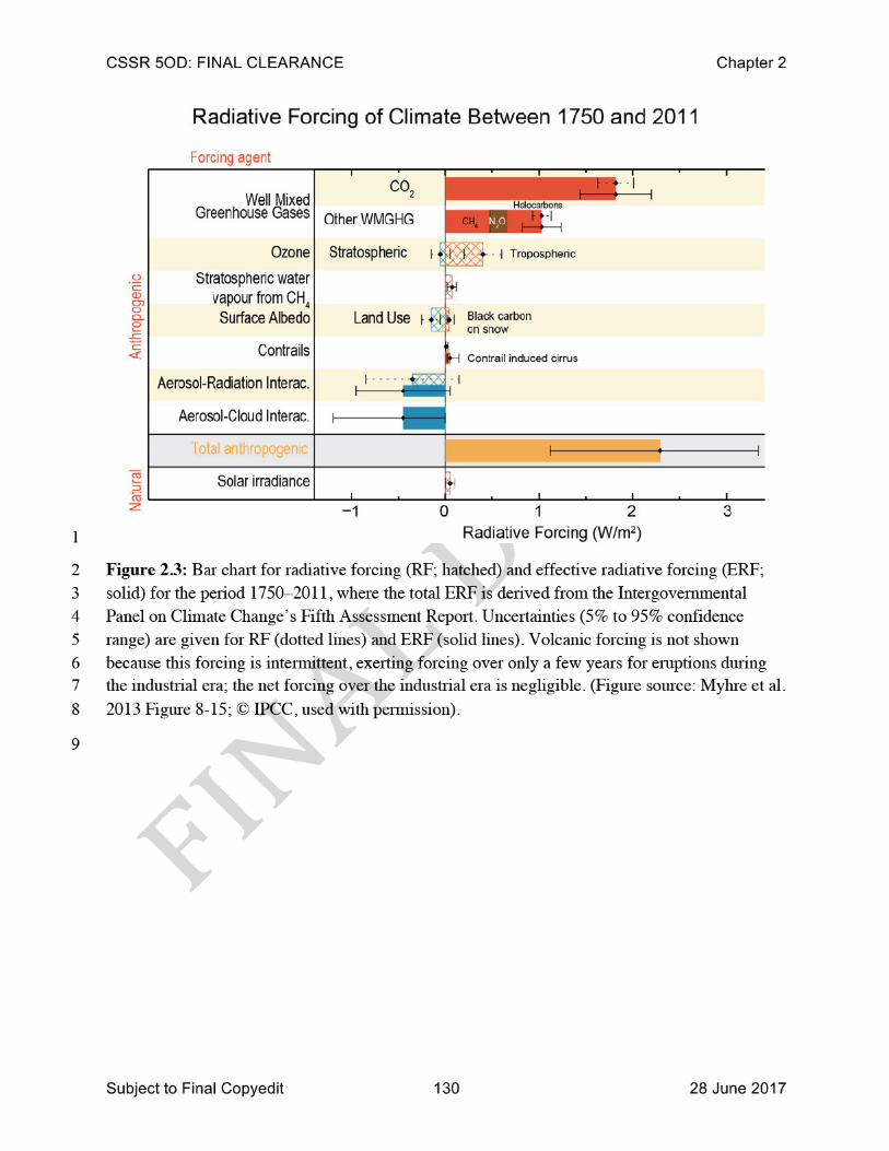
CSSR 50D: FINAL CLEARANCE Chapter 2
Radiative Forcing of Climate Between 1750 and 2011
CO, Wen ~~~i~~ 1 Greenhoose G Other WMGHG
Stratospheric · 1 Tropospheric
Stratospheric
vapour frO;~b~~~ I Surface Land Use f Black carbon
Contrail indJced ClrruS
Aerosol-RadiatKln Inl"rac I
1 Radiative Forcing (W/m2)
2 Figure 2.3: Bar chart for radiative forcing (RF; hatched) and effective radiative forcing (ERF;
3 solid) for die period 1750- 20 11 , where the total ERF is derived from dIe Intergovenunental
4 Panel 0 11 Climate Change 's Fifth Assessment Report. Uncertainties (5% to 95% confidence
5 range) are given for RF (dotted lines) and ERF (solid lines). Volcanic forcing is not shown
6 because this forcing is intennittelll , exerting forcing over only a few years for emptions during 7 the industrial era; the net forcing over the industrial era is negligible . (Figure source: Myhre et al.
8 2013 Figure 8-15 ; © IPCC , used with pennission).
9
Subject to Final Copyedit 130 28 June 2017

1
CSSR 500: FI NAL CLEARANCE Chapter 2
400 400
360 360
E 320 320 ~ • ~ 2BO "N ~
2BO " 0 I \ I I I u
240 .~~ r-\~ ~ ·~tt~ 240
200 200 I " : ~~
160 160 800,000 600,000 400,000 200 ,000 0 1750 1800 1850 1900 1950 2000
2000 ,-------------------------, 2000,-------------------------,
1750
1500
~ 1250
I 1000 u
750
500
1750
1500
1 2~
1000
750 ~ .....
500
250.~ __ ~~----~~--~~--~ 2~~--__ ~--~--~----~~~ BOO.OOO 600.000 400.000 200.000 0 1750 lBOO 1850 1900 1950 2000
~O ~0 r-----------------------,
320
:0 280 ~ ~ 260 o Z 240
220
200 • 1 80 ~ __________________ ~·~ __ ~
800,000 600,000 400,000 200,000 0 Years before 2015
320
300
280
260
240
220
200
• • • •
./
180~ ______________________ ~
1750 1800 1850 1900 1950 2000 Year
2 Figure 2.4: Atmospheric concentrations of CO2 (top) , C~ (middle) , and N20 (bottom) over the 3 last 800,000 years (left panels) and for 1750- 2015 (right panels). Measurements are shown from
4 ice cores (symbols widl different colors for different studies) and for direct atmospheric
5 measurements (red lines). (Adapted from IPee [2007], Figure SPM.1 , © IPCC. used with 6 peffilissioll; data are from https:l/www .epa.gov/climate-indicators/climate-change-indicators-7 atmospheric-concentrations-greenhouse-gases).
Subject to Final Copyedit 131 28 June 20 17


CSSR 5OD: FINAL CLEARANCE Chapter 2
Subject to Final Copyedit 28 June 2017135
REFERENCES 1
ACC-MIP, 2017: Atmospheric Chemistry and Climate MIP. WCRP Working Group on Coupled 2 Modeling. https://www.wcrp-climate.org/modelling-wgcm-mip-catalogue/modelling-wgcm-3 mips-2/226-modelling-wgcm-acc-mip. 4
Allen, M.R. and W.J. Ingram, 2002: Constraints on future changes in climate and the hydrologic 5 cycle. Nature, 419, 224-232. http://dx.doi.org/10.1038/nature01092 6
Alley, K.E., T.A. Scambos, M.R. Siegfried, and H.A. Fricker, 2016: Impacts of warm water on 7 Antarctic ice shelf stability through basal channel formation. Nature Geoscience, 9, 290-293. 8 http://dx.doi.org/10.1038/ngeo2675 9
Anav, A., P. Friedlingstein, M. Kidston, L. Bopp, P. Ciais, P. Cox, C. Jones, M. Jung, R. 10 Myneni, and Z. Zhu, 2013: Evaluating the land and ocean components of the global carbon 11 cycle in the CMIP5 earth system models. Journal of Climate, 26, 6801-6843. 12 http://dx.doi.org/10.1175/jcli-d-12-00417.1 13
Andrews, T., J.M. Gregory, M.J. Webb, and K.E. Taylor, 2012: Forcing, feedbacks and climate 14 sensitivity in CMIP5 coupled atmosphere-ocean climate models. Geophysical Research 15 Letters, 39, L09712. http://dx.doi.org/10.1029/2012GL051607 16
Andronova, N.G., E.V. Rozanov, F. Yang, M.E. Schlesinger, and G.L. Stenchikov, 1999: 17 Radiative forcing by volcanic aerosols from 1850 to 1994. Journal of Geophysical Research: 18 Atmospheres, 104, 16807-16826. 19
Babu, S.S., M.R. Manoj, K.K. Moorthy, M.M. Gogoi, V.S. Nair, S.K. Kompalli, S.K. Satheesh, 20 K. Niranjan, K. Ramagopal, P.K. Bhuyan, and D. Singh, 2013: Trends in aerosol optical 21 depth over Indian region: Potential causes and impact indicators. Journal of Geophysical 22 Research: Atmospheres, 118, 11,794-11,806. http://dx.doi.org/10.1002/2013JD020507 23
Banerjee, A., A.T. Archibald, A.C. Maycock, P. Telford, N.L. Abraham, X. Yang, P. Braesicke, 24 and J.A. Pyle, 2014: Lightning NOx, a key chemistry–climate interaction: Impacts of future 25 climate change and consequences for tropospheric oxidising capacity. Atmospheric 26 Chemistry and Physics, 14, 9871-9881. http://dx.doi.org/10.5194/acp-14-9871-2014 27
Barkstrom, B.R., 1984: The Earth Radiation Budget Experiment (ERBE). Bulletin of the 28 American Meteorological Society, 65, 1170-1185. http://dx.doi.org/10.1175/1520-29 0477(1984)065<1170:terbe>2.0.co;2 30
Behrenfeld, M.J., R.T. O’Malley, D.A. Siegel, C.R. McClain, J.L. Sarmiento, G.C. Feldman, 31 A.J. Milligan, P.G. Falkowski, R.M. Letelier, and E.S. Boss, 2006: Climate-driven trends in 32 contemporary ocean productivity. Nature, 444, 752-755. 33 http://dx.doi.org/10.1038/nature05317 34

CSSR 5OD: FINAL CLEARANCE Chapter 2
Subject to Final Copyedit 28 June 2017136
Bidigare, R.R., F. Chai, M.R. Landry, R. Lukas, C.C.S. Hannides, S.J. Christensen, D.M. Karl, 1 L. Shi, and Y. Chao, 2009: Subtropical ocean ecosystem structure changes forced by North 2 Pacific climate variations. Journal of Plankton Research, 31, 1131-1139. 3 http://dx.doi.org/10.1093/plankt/fbp064 4
Bindoff, N.L., P.A. Stott, K.M. AchutaRao, M.R. Allen, N. Gillett, D. Gutzler, K. Hansingo, G. 5 Hegerl, Y. Hu, S. Jain, I.I. Mokhov, J. Overland, J. Perlwitz, R. Sebbari, and X. Zhang, 2013: 6 Detection and attribution of climate change: From global to regional. Climate Change 2013: 7 The Physical Science Basis. Contribution of Working Group I to the Fifth Assessment Report 8 of the Intergovernmental Panel on Climate Change. Stocker, T.F., D. Qin, G.-K. Plattner, M. 9 Tignor, S.K. Allen, J. Boschung, A. Nauels, Y. Xia, V. Bex, and P.M. Midgley, Eds. 10 Cambridge University Press, Cambridge, United Kingdom and New York, NY, USA, 867–11 952. http://www.climatechange2013.org/report/full-report/ 12
Boer, G. and B. Yu, 2003: Climate sensitivity and response. Climate Dynamics, 20, 415-429. 13 http://dx.doi.org/10.1007/s00382-002-0283-3 14
Bolduc, C., M.S. Bourqui, and P. Charbonneau, 2015: A comparison of stratospheric 15 photochemical response to different reconstructions of solar ultraviolet radiative variability. 16 Journal of Atmospheric and Solar-Terrestrial Physics, 132, 22-32. 17 http://dx.doi.org/10.1016/j.jastp.2015.06.008 18
Bond, T.C., S.J. Doherty, D.W. Fahey, P.M. Forster, T. Berntsen, B.J. DeAngelo, M.G. Flanner, 19 S. Ghan, B. Kärcher, D. Koch, S. Kinne, Y. Kondo, P.K. Quinn, M.C. Sarofim, M.G. 20 Schultz, M. Schulz, C. Venkataraman, H. Zhang, S. Zhang, N. Bellouin, S.K. Guttikunda, 21 P.K. Hopke, M.Z. Jacobson, J.W. Kaiser, Z. Klimont, U. Lohmann, J.P. Schwarz, D. 22 Shindell, T. Storelvmo, S.G. Warren, and C.S. Zender, 2013: Bounding the role of black 23 carbon in the climate system: A scientific assessment. Journal of Geophysical Research: 24 Atmospheres, 118, 5380-5552. http://dx.doi.org/10.1002/jgrd.50171 25
Bony, S., R. Colman, V.M. Kattsov, R.P. Allan, C.S. Bretherton, J.-L. Dufresne, A. Hall, S. 26 Hallegatte, M.M. Holland, W. Ingram, D.A. Randall, B.J. Soden, G. Tselioudis, and M.J. 27 Webb, 2006: How well do we understand and evaluate climate change feedback processes? 28 Journal of Climate, 19, 3445-3482. http://dx.doi.org/10.1175/JCLI3819.1 29
Boucher, O., D. Randall, P. Artaxo, C. Bretherton, G. Feingold, P. Forster, V.-M. Kerminen, Y. 30 Kondo, H. Liao, U. Lohmann, P. Rasch, S.K. Satheesh, S. Sherwood, B. Stevens, and X.Y. 31 Zhang, 2013: Clouds and aerosols. Climate Change 2013: The Physical Science Basis. 32 Contribution of Working Group I to the Fifth Assessment Report of the Intergovernmental 33 Panel on Climate Change. Stocker, T.F., D. Qin, G.-K. Plattner, M. Tignor, S.K. Allen, J. 34 Boschung, A. Nauels, Y. Xia, V. Bex, and P.M. Midgley, Eds. Cambridge University Press, 35 Cambridge, United Kingdom and New York, NY, USA, 571–658. 36 http://www.climatechange2013.org/report/full-report/ 37

CSSR 5OD: FINAL CLEARANCE Chapter 2
Subject to Final Copyedit 28 June 2017137
Boyce, D.G., M.R. Lewis, and B. Worm, 2010: Global phytoplankton decline over the past 1 century. Nature, 466, 591-596. http://dx.doi.org/10.1038/nature09268 2
Brzostek, E.R., J.B. Fisher, and R.P. Phillips, 2014: Modeling the carbon cost of plant nitrogen 3 acquisition: Mycorrhizal trade-offs and multipath resistance uptake improve predictions of 4 retranslocation. Journal of Geophysical Research: Biogeosciences, 119, 1684-1697. 5 http://dx.doi.org/10.1002/2014JG002660 6
Burkhardt, U. and B. Kärcher, 2011: Global radiative forcing from contrail cirrus. Nature 7 Climate Change, 1, 54-58. http://dx.doi.org/10.1038/nclimate1068 8
Capotondi, A., M.A. Alexander, N.A. Bond, E.N. Curchitser, and J.D. Scott, 2012: Enhanced 9 upper ocean stratification with climate change in the CMIP3 models. Journal of Geophysical 10 Research: Oceans, 117, C04031. http://dx.doi.org/10.1029/2011JC007409 11
Carr, M.-E., M.A.M. Friedrichs, M. Schmeltz, M. Noguchi Aita, D. Antoine, K.R. Arrigo, I. 12 Asanuma, O. Aumont, R. Barber, M. Behrenfeld, R. Bidigare, E.T. Buitenhuis, J. Campbell, 13 A. Ciotti, H. Dierssen, M. Dowell, J. Dunne, W. Esaias, B. Gentili, W. Gregg, S. Groom, N. 14 Hoepffner, J. Ishizaka, T. Kameda, C. Le Quéré, S. Lohrenz, J. Marra, F. Mélin, K. Moore, 15 A. Morel, T.E. Reddy, J. Ryan, M. Scardi, T. Smyth, K. Turpie, G. Tilstone, K. Waters, and 16 Y. Yamanaka, 2006: A comparison of global estimates of marine primary production from 17 ocean color. Deep Sea Research Part II: Topical Studies in Oceanography, 53, 741-770. 18 http://dx.doi.org/10.1016/j.dsr2.2006.01.028 19
Carslaw, K.S., L.A. Lee, C.L. Reddington, K.J. Pringle, A. Rap, P.M. Forster, G.W. Mann, D.V. 20 Spracklen, M.T. Woodhouse, L.A. Regayre, and J.R. Pierce, 2013: Large contribution of 21 natural aerosols to uncertainty in indirect forcing. Nature, 503, 67-71. 22 http://dx.doi.org/10.1038/nature12674 23
Chavez, F.P., M. Messié, and J.T. Pennington, 2011: Marine primary production in relation to 24 climate variability and change. Annual Review of Marine Science, 3, 227-260. 25 http://dx.doi.org/10.1146/annurev.marine.010908.163917 26
Chen, T., W.B. Rossow, and Y. Zhang, 2000: Radiative effects of cloud-type variations. Journal 27 of Climate, 13, 264-286. http://dx.doi.org/10.1175/1520-28 0442(2000)013<0264:reoctv>2.0.co;2 29
Chin, M., T. Diehl, Q. Tan, J.M. Prospero, R.A. Kahn, L.A. Remer, H. Yu, A.M. Sayer, H. Bian, 30 I.V. Geogdzhayev, B.N. Holben, S.G. Howell, B.J. Huebert, N.C. Hsu, D. Kim, T.L. 31 Kucsera, R.C. Levy, M.I. Mishchenko, X. Pan, P.K. Quinn, G.L. Schuster, D.G. Streets, S.A. 32 Strode, O. Torres, and X.P. Zhao, 2014: Multi-decadal aerosol variations from 1980 to 2009: 33 A perspective from observations and a global model. Atmospheric Chemistry and Physics, 34 14, 3657-3690. http://dx.doi.org/10.5194/acp-14-3657-2014 35

CSSR 5OD: FINAL CLEARANCE Chapter 2
Subject to Final Copyedit 28 June 2017138
Chiodo, G., D.R. Marsh, R. Garcia-Herrera, N. Calvo, and J.A. García, 2014: On the detection of 1 the solar signal in the tropical stratosphere. Atmospheric Chemistry and Physics, 14, 5251-2 5269. http://dx.doi.org/10.5194/acp-14-5251-2014 3
Ciais, P., C. Sabine, G. Bala, L. Bopp, V. Brovkin, J. Canadell, A. Chhabra, R. DeFries, J. 4 Galloway, M. Heimann, C. Jones, C. Le Quéré, R.B. Myneni, S. Piao, and P. Thornton, 5 2013: Carbon and other biogeochemical cycles. Climate Change 2013: The Physical Science 6 Basis. Contribution of Working Group I to the Fifth Assessment Report of the 7 Intergovernmental Panel on Climate Change. Stocker, T.F., D. Qin, G.-K. Plattner, M. 8 Tignor, S.K. Allen, J. Boschung, A. Nauels, Y. Xia, V. Bex, and P.M. Midgley, Eds. 9 Cambridge University Press, Cambridge, United Kingdom and New York, NY, USA, 465–10 570. http://www.climatechange2013.org/report/full-report/ 11
Clark, P.U., J.D. Shakun, S.A. Marcott, A.C. Mix, M. Eby, S. Kulp, A. Levermann, G.A. Milne, 12 P.L. Pfister, B.D. Santer, D.P. Schrag, S. Solomon, T.F. Stocker, B.H. Strauss, A.J. Weaver, 13 R. Winkelmann, D. Archer, E. Bard, A. Goldner, K. Lambeck, R.T. Pierrehumbert, and G.-14 K. Plattner, 2016: Consequences of twenty-first-century policy for multi-millennial climate 15 and sea-level change. Nature Climate Change, 6, 360-369. 16 http://dx.doi.org/10.1038/nclimate2923 17
Collins, M., R. Knutti, J. Arblaster, J.-L. Dufresne, T. Fichefet, P. Friedlingstein, X. Gao, W.J. 18 Gutowski, T. Johns, G. Krinner, M. Shongwe, C. Tebaldi, A.J. Weaver, and M. Wehner, 19 2013: Long-term climate change: Projections, commitments and irreversibility. Climate 20 Change 2013: The Physical Science Basis. Contribution of Working Group I to the Fifth 21 Assessment Report of the Intergovernmental Panel on Climate Change. Stocker, T.F., D. 22 Qin, G.-K. Plattner, M. Tignor, S.K. Allen, J. Boschung, A. Nauels, Y. Xia, V. Bex, and 23 P.M. Midgley, Eds. Cambridge University Press, Cambridge, United Kingdom and New 24 York, NY, USA, 1029–1136. http://www.climatechange2013.org/report/full-report/ 25
Cook, B.I., S.P. Shukla, M.J. Puma, and L.S. Nazarenko, 2015: Irrigation as an historical climate 26 forcing. Climate Dynamics, 44, 1715-1730. http://dx.doi.org/10.1007/s00382-014-2204-7 27
Crook, J.A. and P.M. Forster, 2011: A balance between radiative forcing and climate feedback in 28 the modeled 20th century temperature response. Journal of Geophysical Research: 29 Atmospheres, 116, n/a-n/a. http://dx.doi.org/10.1029/2011JD015924 30
Davies, J.H. and D.R. Davies, 2010: Earth's surface heat flux. Solid Earth, 1, 5-24. 31 http://dx.doi.org/10.5194/se-1-5-2010 32
Dentener, F., D. Stevenson, J. Cofala, R. Mechler, M. Amann, P. Bergamaschi, F. Raes, and R. 33 Derwent, 2005: The impact of air pollutant and methane emission controls on tropospheric 34 ozone and radiative forcing: CTM calculations for the period 1990-2030. Atmospheric 35 Chemistry and Physics, 5, 1731-1755. http://dx.doi.org/10.5194/acp-5-1731-2005 36

CSSR 5OD: FINAL CLEARANCE Chapter 2
Subject to Final Copyedit 28 June 2017139
Dessler, A.E., M.R. Schoeberl, T. Wang, S.M. Davis, K.H. Rosenlof, and J.P. Vernier, 2014: 1 Variations of stratospheric water vapor over the past three decades. Journal of Geophysical 2 Research: Atmospheres, 119, 12,588-12,598. http://dx.doi.org/10.1002/2014JD021712 3
Dhomse, S.S., M.P. Chipperfield, W. Feng, W.T. Ball, Y.C. Unruh, J.D. Haigh, N.A. Krivova, 4 S.K. Solanki, and A.K. Smith, 2013: Stratospheric O3 changes during 2001–2010: The small 5 role of solar flux variations in a chemical transport model. Atmospheric Chemistry and 6 Physics, 13, 10113-10123. http://dx.doi.org/10.5194/acp-13-10113-2013 7
Dietmüller, S., M. Ponater, and R. Sausen, 2014: Interactive ozone induces a negative feedback 8 in CO2-driven climate change simulations. Journal of Geophysical Research: Atmospheres, 9 119, 1796-1805. http://dx.doi.org/10.1002/2013JD020575 10
Doney, S.C., 2010: The growing human footprint on coastal and open-ocean biogeochemistry. 11 Science, 328, 1512-6. http://dx.doi.org/10.1126/science.1185198 12
Durack, P.J. and S.E. Wijffels, 2010: Fifty-year trends in global ocean salinities and their 13 relationship to broad-scale warming. Journal of Climate, 23, 4342-4362. 14 http://dx.doi.org/10.1175/2010jcli3377.1 15
Enderlin, E.M. and G.S. Hamilton, 2014: Estimates of iceberg submarine melting from high-16 resolution digital elevation models: Application to Sermilik Fjord, East Greenland. Journal 17 of Glaciology, 60, 1084-1092. http://dx.doi.org/10.3189/2014JoG14J085 18
Ermolli, I., K. Matthes, T. Dudok de Wit, N.A. Krivova, K. Tourpali, M. Weber, Y.C. Unruh, L. 19 Gray, U. Langematz, P. Pilewskie, E. Rozanov, W. Schmutz, A. Shapiro, S.K. Solanki, and 20 T.N. Woods, 2013: Recent variability of the solar spectral irradiance and its impact on 21 climate modelling. Atmospheric Chemistry and Physics, 13, 3945-3977. 22 http://dx.doi.org/10.5194/acp-13-3945-2013 23
Falkowski, P.G., M.E. Katz, A.H. Knoll, A. Quigg, J.A. Raven, O. Schofield, and F.J.R. Taylor, 24 2004: The evolution of modern eukaryotic phytoplankton. Science, 305, 354-360. 25 http://dx.doi.org/10.1126/science.1095964 26
Fernandes, R., H. Zhao, X. Wang, J. Key, X. Qu, and A. Hall, 2009: Controls on Northern 27 Hemisphere snow albedo feedback quantified using satellite Earth observations. Geophysical 28 Research Letters, 36, L21702. http://dx.doi.org/10.1029/2009GL040057 29
Fiore, A.M., V. Naik, and E.M. Leibensperger, 2015: Air quality and climate connections. 30 Journal of the Air & Waste Management Association, 65, 645-686. 31 http://dx.doi.org/10.1080/10962247.2015.1040526 32
Flanner, M.G., 2009: Integrating anthropogenic heat flux with global climate models. 33 Geophysical Research Letters, 36, L02801. http://dx.doi.org/10.1029/2008gl036465 34

CSSR 5OD: FINAL CLEARANCE Chapter 2
Subject to Final Copyedit 28 June 2017140
Flanner, M.G., C.S. Zender, P.G. Hess, N.M. Mahowald, T.H. Painter, V. Ramanathan, and P.J. 1 Rasch, 2009: Springtime warming and reduced snow cover from carbonaceous particles. 2 Atmospheric Chemistry and Physics, 9, 2481-2497. http://dx.doi.org/10.5194/acp-9-2481-3 2009 4
Flato, G., J. Marotzke, B. Abiodun, P. Braconnot, S.C. Chou, W. Collins, P. Cox, F. Driouech, S. 5 Emori, V. Eyring, C. Forest, P. Gleckler, E. Guilyardi, C. Jakob, V. Kattsov, C. Reason, and 6 M. Rummukainen, 2013: Evaluation of climate models. Climate Change 2013: The Physical 7 Science Basis. Contribution of Working Group I to the Fifth Assessment Report of the 8 Intergovernmental Panel on Climate Change. Stocker, T.F., D. Qin, G.-K. Plattner, M. 9 Tignor, S.K. Allen, J. Boschung, A. Nauels, Y. Xia, V. Bex, and P.M. Midgley, Eds. 10 Cambridge University Press, Cambridge, United Kingdom and New York, NY, USA, 741–11 866. http://www.climatechange2013.org/report/full-report/ 12
Floyd, L.E., J.W. Cook, L.C. Herring, and P.C. Crane, 2003: SUSIM'S 11-year observational 13 record of the solar UV irradiance. Advances in Space Research, 31, 2111-2120. 14 http://dx.doi.org/10.1016/S0273-1177(03)00148-0 15
Forster, P., V. Ramaswamy, P. Artaxo, T. Berntsen, R. Betts, D.W. Fahey, J. Haywood, J. Lean, 16 D.C. Lowe, G. Myhre, J. Nganga, R. Prinn, G. Raga, M. Schulz, and R. Van Dorland, 2007: 17 Ch. 2: Changes in atmospheric constituents and in radiative forcing. Climate Change 2007: 18 The Physical Science Basis. Contribution of Working Group I to the Fourth Assessment 19 Report (AR4) of the Intergovernmental Panel on Climate Change. Solomon, S., D. Qin, M. 20 Manning, Z. Chen, M. Marquis, K.B. Averyt, M. Tignor, and H.L. Miller, Eds. Cambridge 21 University Press, Cambridge, UK. 22 http://www.ipcc.ch/publications_and_data/ar4/wg1/en/ch2.html 23
Fowler, D., M. Coyle, U. Skiba, M.A. Sutton, J.N. Cape, S. Reis, L.J. Sheppard, A. Jenkins, B. 24 Grizzetti, J.N. Galloway, P. Vitousek, A. Leach, A.F. Bouwman, K. Butterbach-Bahl, F. 25 Dentener, D. Stevenson, M. Amann, and M. Voss, 2013: The global nitrogen cycle in the 26 twenty-first century. Philosophical Transactions of the Royal Society B: Biological Sciences, 27 368, 20130164. http://dx.doi.org/10.1098/rstb.2013.0164 28
Franks, P.J., M.A. Adams, J.S. Amthor, M.M. Barbour, J.A. Berry, D.S. Ellsworth, G.D. 29 Farquhar, O. Ghannoum, J. Lloyd, N. McDowell, R.J. Norby, D.T. Tissue, and S. von 30 Caemmerer, 2013: Sensitivity of plants to changing atmospheric CO2 concentration: From 31 the geological past to the next century. New Phytologist, 197, 1077-1094. 32 http://dx.doi.org/10.1111/nph.12104 33
Friedlingstein, P., P. Cox, R. Betts, L. Bopp, W.v. Bloh, V. Brovkin, P. Cadule, S. Doney, M. 34 Eby, I. Fung, G. Bala, J. John, C. Jones, F. Joos, T. Kato, M. Kawamiya, W. Knorr, K. 35 Lindsay, H.D. Matthews, T. Raddatz, P. Rayner, C. Reick, E. Roeckner, K.-G. Schnitzler, R. 36 Schnur, K. Strassmann, A.J. Weaver, C. Yoshikawa, and N. Zeng, 2006: Climate–carbon 37

CSSR 5OD: FINAL CLEARANCE Chapter 2
Subject to Final Copyedit 28 June 2017141
cycle feedback analysis: Results from the C4MIP model intercomparison. Journal of Climate, 1 19, 3337-3353. http://dx.doi.org/10.1175/JCLI3800.1 2
Friedlingstein, P., M. Meinshausen, V.K. Arora, C.D. Jones, A. Anav, S.K. Liddicoat, and R. 3 Knutti, 2014: Uncertainties in CMIP5 climate projections due to carbon cycle feedbacks. 4 Journal of Climate, 27, 511-526. http://dx.doi.org/10.1175/JCLI-D-12-00579.1 5
Fröhlich, C. and J. Lean, 2004: Solar radiative output and its variability: Evidence and 6 mechanisms. The Astronomy and Astrophysics Review, 12, 273-320. 7 http://dx.doi.org/10.1007/s00159-004-0024-1 8
Frölicher, T.L., K.B. Rodgers, C.A. Stock, and W.W.L. Cheung, 2016: Sources of uncertainties 9 in 21st century projections of potential ocean ecosystem stressors. Global Biogeochemical 10 Cycles, 30, 1224-1243. http://dx.doi.org/10.1002/2015GB005338 11
Fu, W., J.T. Randerson, and J.K. Moore, 2016: Climate change impacts on net primary 12 production (NPP) and export production (EP) regulated by increasing stratification and 13 phytoplankton community structure in the CMIP5 models. Biogeosciences, 13, 5151-5170. 14 http://dx.doi.org/10.5194/bg-13-5151-2016 15
Gao, F.-L., L.-R. Tao, G.-M. Cui, J.-L. Xu, and T.-C. Hua, 2015: The influence of solar spectral 16 variations on global radiative balance. Advances in Space Research, 55, 682-687. 17 http://dx.doi.org/10.1016/j.asr.2014.10.028 18
Gelderloos, R., F. Straneo, and C.A. Katsman, 2012: Mechanisms behind the temporary 19 shutdown of deep convection in the Labrador Sea: Lessons from the great salinity anomaly 20 years 1968–71. Journal of Climate, 25, 6743-6755. http://dx.doi.org/10.1175/jcli-d-11-21 00549.1 22
Gerlach, T., 2011: Volcanic versus anthropogenic carbon dioxide. Eos, Transactions, American 23 Geophysical Union, 92, 201-202. http://dx.doi.org/10.1029/2011EO240001 24
Gillett, N.P., M.F. Wehner, S.F.B. Tett, and A.J. Weaver, 2004: Testing the linearity of the 25 response to combined greenhouse gas and sulfate aerosol forcing. Geophysical Research 26 Letters, 31, L14201. http://dx.doi.org/10.1029/2004GL020111 27
González-Eguino, M. and M.B. Neumann, 2016: Significant implications of permafrost thawing 28 for climate change control. Climatic Change, 136, 381-388. 29 http://dx.doi.org/10.1007/s10584-016-1666-5 30
Good, P., J.M. Gregory, J.A. Lowe, and T. Andrews, 2013: Abrupt CO2 experiments as tools for 31 predicting and understanding CMIP5 representative concentration pathway projections. 32 Climate Dynamics, 40, 1041-1053. http://dx.doi.org/10.1007/s00382-012-1410-4 33

CSSR 5OD: FINAL CLEARANCE Chapter 2
Subject to Final Copyedit 28 June 2017142
Gray, L.J., J. Beer, M. Geller, J.D. Haigh, M. Lockwood, K. Matthes, U. Cubasch, D. Fleitmann, 1 G. Harrison, L. Hood, J. Luterbacher, G.A. Meehl, D. Shindell, B. van Geel, and W. White, 2 2010: Solar influences on climate. Reviews of Geophysics, 48, RG4001. 3 http://dx.doi.org/10.1029/2009RG000282 4
Hall, A., 2004: The role of surface albedo feedback in climate. Journal of Climate, 17, 1550-5 1568. http://dx.doi.org/10.1175/1520-0442(2004)017<1550:TROSAF>2.0.CO;2 6
Hall, A. and X. Qu, 2006: Using the current seasonal cycle to constrain snow albedo feedback in 7 future climate change. Geophysical Research Letters, 33, L03502. 8 http://dx.doi.org/10.1029/2005GL025127 9
Han, Z., J. Li, W. Guo, Z. Xiong, and W. Zhang, 2013: A study of dust radiative feedback on 10 dust cycle and meteorology over East Asia by a coupled regional climate-chemistry-aerosol 11 model. Atmospheric Environment, 68, 54-63. 12 http://dx.doi.org/10.1016/j.atmosenv.2012.11.032 13
Hansen, J. and L. Nazarenko, 2004: Soot climate forcing via snow and ice albedos. Proceedings 14 of the National Academy of Sciences of the United States of America, 101, 423-428. 15 http://dx.doi.org/10.1073/pnas.2237157100 16
Hartmann, D.L., M.E. Ockert-Bell, and M.L. Michelsen, 1992: The effect of cloud type on 17 Earth's energy balance: Global analysis. Journal of Climate, 5, 1281-1304. 18 http://dx.doi.org/10.1175/1520-0442(1992)005<1281:teocto>2.0.co;2 19
Hartmann, D.L., A.M.G. Klein Tank, M. Rusticucci, L.V. Alexander, S. Brönnimann, Y. 20 Charabi, F.J. Dentener, E.J. Dlugokencky, D.R. Easterling, A. Kaplan, B.J. Soden, P.W. 21 Thorne, M. Wild, and P.M. Zhai, 2013: Observations: Atmosphere and surface. Climate 22 Change 2013: The Physical Science Basis. Contribution of Working Group I to the Fifth 23 Assessment Report of the Intergovernmental Panel on Climate Change. Stocker, T.F., D. 24 Qin, G.-K. Plattner, M. Tignor, S.K. Allen, J. Boschung, A. Nauels, Y. Xia, V. Bex, and 25 P.M. Midgley, Eds. Cambridge University Press, Cambridge, United Kingdom and New 26 York, NY, USA, 159–254. http://www.climatechange2013.org/report/full-report/ 27
Hauglustaine, D.A., J. Lathière, S. Szopa, and G.A. Folberth, 2005: Future tropospheric ozone 28 simulated with a climate-chemistry-biosphere model. Geophysical Research Letters, 32, 29 L24807. http://dx.doi.org/10.1029/2005GL024031 30
Hegglin, M.I., D.A. Plummer, T.G. Shepherd, J.F. Scinocca, J. Anderson, L. Froidevaux, B. 31 Funke, D. Hurst, A. Rozanov, J. Urban, T. von Clarmann, K.A. Walker, H.J. Wang, S. 32 Tegtmeier, and K. Weigel, 2014: Vertical structure of stratospheric water vapour trends 33 derived from merged satellite data. Nature Geoscience, 7, 768-776. 34 http://dx.doi.org/10.1038/ngeo2236 35

CSSR 5OD: FINAL CLEARANCE Chapter 2
Subject to Final Copyedit 28 June 2017143
Held, I.M. and B.J. Soden, 2000: Water vapor feedback and global warming. Annual Review of 1 Energy and the Environment, 25, 441-475. 2 http://dx.doi.org/10.1146/annurev.energy.25.1.441 3
Hibbard, K.A., G.A. Meehl, P.M. Cox, and P. Friedlingstein, 2007: A strategy for climate change 4 stabilization experiments. Eos, Transactions, American Geophysical Union, 88, 217-221. 5 http://dx.doi.org/10.1029/2007EO200002 6
Holland, D.M., R.H. Thomas, B. de Young, M.H. Ribergaard, and B. Lyberth, 2008: 7 Acceleration of Jakobshavn Isbrae triggered by warm subsurface ocean waters. Nature 8 Geoscience, 1, 659-664. http://dx.doi.org/10.1038/ngeo316 9
Holmes, C.D., M.J. Prather, O.A. Søvde, and G. Myhre, 2013: Future methane, hydroxyl, and 10 their uncertainties: Key climate and emission parameters for future predictions. Atmospheric 11 Chemistry and Physics, 13, 285-302. http://dx.doi.org/10.5194/acp-13-285-2013 12
Hsu, N.C., R. Gautam, A.M. Sayer, C. Bettenhausen, C. Li, M.J. Jeong, S.C. Tsay, and B.N. 13 Holben, 2012: Global and regional trends of aerosol optical depth over land and ocean using 14 SeaWiFS measurements from 1997 to 2010. Atmospheric Chemistry and Physics, 12, 8037-15 8053. http://dx.doi.org/10.5194/acp-12-8037-2012 16
IPCC, 2007: Climate Change 2007: The Physical Science Basis. Contribution of Working Group 17 I to the Fourth Assessment Report of the Intergovernmental Panel on Climate Change. 18 Solomon, S., D. Qin, M. Manning, Z. Chen, M. Marquis, K.B. Averyt, M. Tignor, and H.L. 19 Miller, Eds. Cambridge University Press, Cambridge. U.K, New York, NY, USA, 996 pp. 20 http://www.ipcc.ch/publications_and_data/publications_ipcc_fourth_assessment_report_wg121 _report_the_physical_science_basis.htm 22
IPCC, 2013: Climate Change 2013: The Physical Science Basis. Contribution of Working Group 23 I to the Fifth Assessment Report of the Intergovernmental Panel on Climate Change. 24 Cambridge University Press, Cambridge, UK and New York, NY, 1535 pp. 25 http://www.climatechange2013.org/report/ 26
Isaksen, I., T. Berntsen, S. Dalsøren, K. Eleftheratos, Y. Orsolini, B. Rognerud, F. Stordal, O. 27 Søvde, C. Zerefos, and C. Holmes, 2014: Atmospheric ozone and methane in a changing 28 climate. Atmosphere, 5, 518. http://dx.doi.org/10.3390/atmos5030518 29
Jacobson, M.Z., 2004: Climate response of fossil fuel and biofuel soot, accounting for soot's 30 feedback to snow and sea ice albedo and emissivity. Journal of Geophysical Research, 109, 31 D21201. http://dx.doi.org/10.1029/2004JD004945 32
Jiang, X., S.J. Eichelberger, D.L. Hartmann, R. Shia, and Y.L. Yung, 2007: Influence of doubled 33 CO2 on ozone via changes in the Brewer–Dobson circulation. Journal of the Atmospheric 34 Sciences, 64, 2751-2755. http://dx.doi.org/10.1175/jas3969.1 35

CSSR 5OD: FINAL CLEARANCE Chapter 2
Subject to Final Copyedit 28 June 2017144
Jiao, C., M.G. Flanner, Y. Balkanski, S.E. Bauer, N. Bellouin, T.K. Berntsen, H. Bian, K.S. 1 Carslaw, M. Chin, N. De Luca, T. Diehl, S.J. Ghan, T. Iversen, A. Kirkevåg, D. Koch, X. 2 Liu, G.W. Mann, J.E. Penner, G. Pitari, M. Schulz, Ø. Seland, R.B. Skeie, S.D. Steenrod, P. 3 Stier, T. Takemura, K. Tsigaridis, T. van Noije, Y. Yun, and K. Zhang, 2014: An AeroCom 4 assessment of black carbon in Arctic snow and sea ice. Atmospheric Chemistry and Physics, 5 14, 2399-2417. http://dx.doi.org/10.5194/acp-14-2399-2014 6
Jin, X., N. Gruber, J.P. Dunne, J.L. Sarmiento, and R.A. Armstrong, 2006: Diagnosing the 7 contribution of phytoplankton functional groups to the production and export of particulate 8 organic carbon, CaCO3, and opal from global nutrient and alkalinity distributions. Global 9 Biogeochemical Cycles, 20, GB2015. http://dx.doi.org/10.1029/2005GB002532 10
John, J.G., A.M. Fiore, V. Naik, L.W. Horowitz, and J.P. Dunne, 2012: Climate versus emission 11 drivers of methane lifetime against loss by tropospheric OH from 1860–2100. Atmospheric 12 Chemistry and Physics, 12, 12021-12036. http://dx.doi.org/10.5194/acp-12-12021-2012 13
Johnson, G.C., J.M. Lyman, T. Boyer, C.M. Domingues, M. Ishii, R. Killick, D. Monselesan, 14 and S.E. Wijffels, 2016: [Global Oceans] Ocean heat content [in “State of the Climate in 15 2015”]. Bulletin of the American Meteorological Society, 97, S66-S70. 16 http://dx.doi.org/10.1175/2016BAMSStateoftheClimate.1 17
Jones, A., J.M. Haywood, and O. Boucher, 2007: Aerosol forcing, climate response and climate 18 sensitivity in the Hadley Centre climate model. Journal of Geophysical Research, 112, 19 D20211. http://dx.doi.org/10.1029/2007JD008688 20
Joughin, I., R.B. Alley, and D.M. Holland, 2012: Ice-sheet response to oceanic forcing. Science, 21 338, 1172-1176. http://dx.doi.org/10.1126/science.1226481 22
Ju, J. and J.G. Masek, 2016: The vegetation greenness trend in Canada and US Alaska from 23 1984–2012 Landsat data. Remote Sensing of Environment, 176, 1-16. 24 http://dx.doi.org/10.1016/j.rse.2016.01.001 25
Kay, J.E. and A. Gettelman, 2009: Cloud influence on and response to seasonal Arctic sea ice 26 loss. Journal of Geophysical Research, 114, D18204. 27 http://dx.doi.org/10.1029/2009JD011773 28
Kay, J.E. and T. L'Ecuyer, 2013: Observational constraints on Arctic Ocean clouds and radiative 29 fluxes during the early 21st century. Journal of Geophysical Research: Atmospheres, 118, 30 7219-7236. http://dx.doi.org/10.1002/jgrd.50489 31
Kay, J.E., K. Raeder, A. Gettelman, and J. Anderson, 2011: The boundary layer response to 32 recent Arctic sea ice loss and implications for high-latitude climate feedbacks. Journal of 33 Climate, 24, 428-447. http://dx.doi.org/10.1175/2010JCLI3651.1 34

CSSR 5OD: FINAL CLEARANCE Chapter 2
Subject to Final Copyedit 28 June 2017145
Klocke, D., J. Quaas, and B. Stevens, 2013: Assessment of different metrics for physical climate 1 feedbacks. Climate Dynamics, 41, 1173-1185. http://dx.doi.org/10.1007/s00382-013-1757-1 2
Knutti, R. and G.C. Hegerl, 2008: The equilibrium sensitivity of the Earth’s temperature to 3 radiation changes. Nature Geoscience, 1, 735-743. http://dx.doi.org/10.1038/ngeo337 4
Knutti, R. and M.A.A. Rugenstein, 2015: Feedbacks, climate sensitivity and the limits of linear 5 models. Philosophical Transactions of the Royal Society A: Mathematical, Physical and 6 Engineering Sciences, 373. http://dx.doi.org/10.1098/rsta.2015.0146 7
Koffi, B., M. Schulz, F.-M. Bréon, F. Dentener, B.M. Steensen, J. Griesfeller, D. Winker, Y. 8 Balkanski, S.E. Bauer, N. Bellouin, T. Berntsen, H. Bian, M. Chin, T. Diehl, R. Easter, S. 9 Ghan, D.A. Hauglustaine, T. Iversen, A. Kirkevåg, X. Liu, U. Lohmann, G. Myhre, P. Rasch, 10 Ø. Seland, R.B. Skeie, S.D. Steenrod, P. Stier, J. Tackett, T. Takemura, K. Tsigaridis, M.R. 11 Vuolo, J. Yoon, and K. Zhang, 2016: Evaluation of the aerosol vertical distribution in global 12 aerosol models through comparison against CALIOP measurements: AeroCom phase II 13 results. Journal of Geophysical Research: Atmospheres, 121, 7254-7283. 14 http://dx.doi.org/10.1002/2015JD024639 15
Kopp, G., 2014: An assessment of the solar irradiance record for climate studies. Journal of 16 Space Weather and Space Climate, 4, A14. http://dx.doi.org/10.1051/swsc/2014012 17
Kopp, G. and J.L. Lean, 2011: A new, lower value of total solar irradiance: Evidence and climate 18 significance. Geophysical Research Letters, 38, L01706. 19 http://dx.doi.org/10.1029/2010GL045777 20
Kopp, G., N. Krivova, C.J. Wu, and J. Lean, 2016: The impact of the revised sunspot record on 21 solar irradiance reconstructions. Solar Physics, 291, 2951-1965. 22 http://dx.doi.org/10.1007/s11207-016-0853-x 23
Kostov, Y., K.C. Armour, and J. Marshall, 2014: Impact of the Atlantic meridional overturning 24 circulation on ocean heat storage and transient climate change. Geophysical Research 25 Letters, 41, 2108-2116. http://dx.doi.org/10.1002/2013GL058998 26
Koven, C.D., E.A.G. Schuur, C. Schädel, T.J. Bohn, E.J. Burke, G. Chen, X. Chen, P. Ciais, G. 27 Grosse, J.W. Harden, D.J. Hayes, G. Hugelius, E.E. Jafarov, G. Krinner, P. Kuhry, D.M. 28 Lawrence, A.H. MacDougall, S.S. Marchenko, A.D. McGuire, S.M. Natali, D.J. Nicolsky, D. 29 Olefeldt, S. Peng, V.E. Romanovsky, K.M. Schaefer, J. Strauss, C.C. Treat, and M. Turetsky, 30 2015a: A simplified, data-constrained approach to estimate the permafrost carbon–climate 31 feedback. Philosophical Transactions of the Royal Society A: Mathematical, Physical and 32 Engineering Sciences, 373. http://dx.doi.org/10.1098/rsta.2014.0423 33
Koven, C.D., D.M. Lawrence, and W.J. Riley, 2015b: Permafrost carbon−climate feedback is 34 sensitive to deep soil carbon decomposability but not deep soil nitrogen dynamics. 35

CSSR 5OD: FINAL CLEARANCE Chapter 2
Subject to Final Copyedit 28 June 2017146
Proceedings of the National Academy of Sciences, 112, 3752-3757. 1 http://dx.doi.org/10.1073/pnas.1415123112 2
Krishna Moorthy, K., S. Suresh Babu, M.R. Manoj, and S.K. Satheesh, 2013: Buildup of 3 aerosols over the Indian Region. Geophysical Research Letters, 40, 1011-1014. 4 http://dx.doi.org/10.1002/grl.50165 5
Krissansen-Totton, J. and R. Davies, 2013: Investigation of cosmic ray–cloud connections using 6 MISR. Geophysical Research Letters, 40, 5240-5245. http://dx.doi.org/10.1002/grl.50996 7
Kühn, T., A.I. Partanen, A. Laakso, Z. Lu, T. Bergman, S. Mikkonen, H. Kokkola, H. Korhonen, 8 P. Räisänen, D.G. Streets, S. Romakkaniemi, and A. Laaksonen, 2014: Climate impacts of 9 changing aerosol emissions since 1996. Geophysical Research Letters, 41, 4711-4718. 10 http://dx.doi.org/10.1002/2014GL060349 11
Lacis, A.A., G.A. Schmidt, D. Rind, and R.A. Ruedy, 2010: Atmospheric CO2: Principal control 12 knob governing Earth’s temperature. Science, 330, 356-359. 13 http://dx.doi.org/10.1126/science.1190653 14
Langmann, B., 2014: On the role of climate forcing by volcanic sulphate and volcanic ash. 15 Advances in Meteorology, 2014, 17. http://dx.doi.org/10.1155/2014/340123 16
Laufkötter, C., M. Vogt, N. Gruber, M. Aita-Noguchi, O. Aumont, L. Bopp, E. Buitenhuis, S.C. 17 Doney, J. Dunne, T. Hashioka, J. Hauck, T. Hirata, J. John, C. Le Quéré, I.D. Lima, H. 18 Nakano, R. Seferian, I. Totterdell, M. Vichi, and C. Völker, 2015: Drivers and uncertainties 19 of future global marine primary production in marine ecosystem models. Biogeosciences, 12, 20 6955-6984. http://dx.doi.org/10.5194/bg-12-6955-2015 21
Le Quéré, C., R.M. Andrew, J.G. Canadell, S. Sitch, J.I. Korsbakken, G.P. Peters, A.C. Manning, 22 T.A. Boden, P.P. Tans, R.A. Houghton, R.F. Keeling, S. Alin, O.D. Andrews, P. Anthoni, L. 23 Barbero, L. Bopp, F. Chevallier, L.P. Chini, P. Ciais, K. Currie, C. Delire, S.C. Doney, P. 24 Friedlingstein, T. Gkritzalis, I. Harris, J. Hauck, V. Haverd, M. Hoppema, K. Klein 25 Goldewijk, A.K. Jain, E. Kato, A. Körtzinger, P. Landschützer, N. Lefèvre, A. Lenton, S. 26 Lienert, D. Lombardozzi, J.R. Melton, N. Metzl, F. Millero, P.M.S. Monteiro, D.R. Munro, 27 J.E.M.S. Nabel, S.I. Nakaoka, K. O'Brien, A. Olsen, A.M. Omar, T. Ono, D. Pierrot, B. 28 Poulter, C. Rödenbeck, J. Salisbury, U. Schuster, J. Schwinger, R. Séférian, I. Skjelvan, B.D. 29 Stocker, A.J. Sutton, T. Takahashi, H. Tian, B. Tilbrook, I.T. van der Laan-Luijkx, G.R. van 30 der Werf, N. Viovy, A.P. Walker, A.J. Wiltshire, and S. Zaehle, 2016: Global carbon budget 31 2016. Earth System Science Data, 8, 605-649. http://dx.doi.org/10.5194/essd-8-605-2016 32
le Texier, H., S. Solomon, and R.R. Garcia, 1988: The role of molecular hydrogen and methane 33 oxidation in the water vapour budget of the stratosphere. Quarterly Journal of the Royal 34 Meteorological Society, 114, 281-295. http://dx.doi.org/10.1002/qj.49711448002 35

CSSR 5OD: FINAL CLEARANCE Chapter 2
Subject to Final Copyedit 28 June 2017147
Lean, J., 1997: The sun's variable radiation and its relevance for earth. Annual Review of 1 Astronomy and Astrophysics, 35, 33-67. http://dx.doi.org/10.1146/annurev.astro.35.1.33 2
Leibensperger, E.M., L.J. Mickley, D.J. Jacob, W.T. Chen, J.H. Seinfeld, A. Nenes, P.J. Adams, 3 D.G. Streets, N. Kumar, and D. Rind, 2012: Climatic effects of 1950-2050 changes in US 4 anthropogenic aerosols – Part 1: Aerosol trends and radiative forcing. Atmospheric Chemistry 5 and Physics 12, 3333-3348. http://dx.doi.org/10.5194/acp-12-3333-2012 6
Lelieveld, J. and P.J. Crutzen, 1992: Indirect chemical effects of methane on climate warming. 7 Nature, 355, 339-342. http://dx.doi.org/10.1038/355339a0 8
Li, F., J. Austin, and J. Wilson, 2008: The strength of the Brewer–Dobson circulation in a 9 changing climate: Coupled chemistry–climate model simulations. Journal of Climate, 21, 40-10 57. http://dx.doi.org/10.1175/2007jcli1663.1 11
Li, J., Z. Han, and Z. Xie, 2013: Model analysis of long-term trends of aerosol concentrations 12 and direct radiative forcings over East Asia. Tellus B: Chemical and Physical Meteorology, 13 65, 20410. http://dx.doi.org/10.3402/tellusb.v65i0.20410 14
Liao, H., Y. Zhang, W.-T. Chen, F. Raes, and J.H. Seinfeld, 2009: Effect of chemistry-aerosol-15 climate coupling on predictions of future climate and future levels of tropospheric ozone and 16 aerosols. Journal of Geophysical Research: Atmospheres, 114, D10306. 17 http://dx.doi.org/10.1029/2008JD010984 18
Liljedahl, A.K., J. Boike, R.P. Daanen, A.N. Fedorov, G.V. Frost, G. Grosse, L.D. Hinzman, Y. 19 Iijma, J.C. Jorgenson, N. Matveyeva, M. Necsoiu, M.K. Raynolds, V.E. Romanovsky, J. 20 Schulla, K.D. Tape, D.A. Walker, C.J. Wilson, H. Yabuki, and D. Zona, 2016: Pan-Arctic 21 ice-wedge degradation in warming permafrost and its influence on tundra hydrology. Nature 22 Geoscience, 9, 312-318. http://dx.doi.org/10.1038/ngeo2674 23
Lockwood, M., 2012: Solar influence on global and regional climates. Surveys in Geophysics, 24 33, 503-534. http://dx.doi.org/10.1007/s10712-012-9181-3 25
Loeb, N. G., S. Kato and B. A. Wielicki, 2002: Defining Top-of-the-Atmosphere Flux Reference 26 Level for Earth Radiation Budget Studies, Journal of Climate, 15, 3301-27 3309, http://dx.doi.org/10.1175/1520-0442(2002)015<3301:DTOTAF>2.0.CO;2 28
Loeb, N.G., B.A. Wielicki, D.R. Doelling, G.L. Smith, D.F. Keyes, S. Kato, N. Manalo-Smith, 29 and T. Wong, 2009: Toward optimal closure of the Earth's top-of-atmosphere radiation 30 budget. Journal of Climate, 22, 748-766. http://dx.doi.org/10.1175/2008JCLI2637.1 31
Löffler, M., S. Brinkop, and P. Jöckel, 2016: Impact of major volcanic eruptions on stratospheric 32 water vapour. Atmospheric Chemistry and Physics, 16, 6547-6562. 33 http://dx.doi.org/10.5194/acp-16-6547-2016 34

CSSR 5OD: FINAL CLEARANCE Chapter 2
Subject to Final Copyedit 28 June 2017148
Lohmann, U. and J. Feichter, 2005: Global indirect aerosol effects: A review. Atmospheric 1 Chemistry and Physics, 5, 715-737. http://dx.doi.org/10.5194/acp-5-715-2005 2
Lynch, P., J.S. Reid, D.L. Westphal, J. Zhang, T.F. Hogan, E.J. Hyer, C.A. Curtis, D.A. Hegg, Y. 3 Shi, J.R. Campbell, J.I. Rubin, W.R. Sessions, F.J. Turk, and A.L. Walker, 2016: An 11-year 4 global gridded aerosol optical thickness reanalysis (v1.0) for atmospheric and climate 5 sciences. Geoscientific Model Development, 9, 1489-1522. http://dx.doi.org/10.5194/gmd-9-6 1489-2016 7
Mahajan, S., K.J. Evans, J.J. Hack, and J.E. Truesdale, 2013: Linearity of climate response to 8 increases in black carbon aerosols. Journal of Climate, 26, 8223-8237. 9 http://dx.doi.org/10.1175/JCLI-D-12-00715.1 10
Mao, J., A. Ribes, B. Yan, X. Shi, P.E. Thornton, R. Seferian, P. Ciais, R.B. Myneni, H. 11 Douville, S. Piao, Z. Zhu, R.E. Dickinson, Y. Dai, D.M. Ricciuto, M. Jin, F.M. Hoffman, B. 12 Wang, M. Huang, and X. Lian, 2016: Human-induced greening of the northern extratropical 13 land surface. Nature Climate Change, 6, 959-963. http://dx.doi.org/10.1038/nclimate3056 14
Mao, K.B., Y. Ma, L. Xia, W.Y. Chen, X.Y. Shen, T.J. He, and T.R. Xu, 2014: Global aerosol 15 change in the last decade: An analysis based on MODIS data. Atmospheric Environment, 94, 16 680-686. http://dx.doi.org/10.1016/j.atmosenv.2014.04.053 17
Marmer, E., B. Langmann, H. Fagerli, and V. Vestreng, 2007: Direct shortwave radiative forcing 18 of sulfate aerosol over Europe from 1900 to 2000. Journal of Geophysical Research, 112, 19 D23S17. http://dx.doi.org/10.1029/2006JD008037 20
Masson-Delmotte, V., M. Schulz, A. Abe-Ouchi, J. Beer, A. Ganopolski, J.F. González Rouco, 21 E. Jansen, K. Lambeck, J. Luterbacher, T. Naish, T. Osborn, B. Otto-Bliesner, T. Quinn, R. 22 Ramesh, M. Rojas, X. Shao, and A. Timmermann, 2013: Information from paleoclimate 23 archives. Climate Change 2013: The Physical Science Basis. Contribution of Working Group 24 I to the Fifth Assessment Report of the Intergovernmental Panel on Climate Change. Stocker, 25 T.F., D. Qin, G.-K. Plattner, M. Tignor, S.K. Allen, J. Boschung, A. Nauels, Y. Xia, V. Bex, 26 and P.M. Midgley, Eds. Cambridge University Press, Cambridge, United Kingdom and New 27 York, NY, USA, 383–464. http://www.climatechange2013.org/report/full-report/ 28
Matthews, H.D., A.J. Weaver, K.J. Meissner, N.P. Gillett, and M. Eby, 2004: Natural and 29 anthropogenic climate change: Incorporating historical land cover change, vegetation 30 dynamics and the global carbon cycle. Climate Dynamics, 22, 461-479. 31 http://dx.doi.org/10.1007/s00382-004-0392-2 32
McLandress, C., T.G. Shepherd, M.C. Reader, D.A. Plummer, and K.P. Shine, 2014: The climate 33 impact of past changes in halocarbons and CO2 in the tropical UTLS region. Journal of 34 Climate, 27, 8646-8660. http://dx.doi.org/10.1175/jcli-d-14-00232.1 35
CSSR 5OD: FINAL CLEARANCE Chapter 2
Subject to Final Copyedit 28 June 2017149
Meehl, G.A., W.M. Washington, C.M. Ammann, J.M. Arblaster, T.M.L. Wigley, and C. Tebaldi, 1 2004: Combinations of natural and anthropogenic forcings in twentieth-century climate. 2 Journal of Climate, 17, 3721-3727. http://dx.doi.org/10.1175/1520-3 0442(2004)017<3721:CONAAF>2.0.CO;2 4
Melillo, J.M., T.C. Richmond, and G.W. Yohe, eds., 2014: Climate Change Impacts in the 5 United States: The Third National Climate Assessment. U.S. Global Change Research 6 Program: Washington, D.C., 842 pp. http://dx.doi.org/10.7930/J0Z31WJ2 7
Morgenstern, O., G. Zeng, N. Luke Abraham, P.J. Telford, P. Braesicke, J.A. Pyle, S.C. 8 Hardiman, F.M. O'Connor, and C.E. Johnson, 2013: Impacts of climate change, ozone 9 recovery, and increasing methane on surface ozone and the tropospheric oxidizing capacity. 10 Journal of Geophysical Research: Atmospheres, 118, 1028-1041. 11 http://dx.doi.org/10.1029/2012JD018382 12
Morris, G.A., J.E. Rosenfield, M.R. Schoeberl, and C.H. Jackman, 2003: Potential impact of 13 subsonic and supersonic aircraft exhaust on water vapor in the lower stratosphere assessed 14 via a trajectory model. Journal of Geophysical Research: Atmospheres, 108, 4103. 15 http://dx.doi.org/10.1029/2002JD002614 16
Munk, W. and C. Wunsch, 1998: Abyssal recipes II: Energetics of tidal and wind mixing. Deep 17 Sea Research Part I: Oceanographic Research Papers, 45, 1977-2010. 18 http://dx.doi.org/10.1016/S0967-0637(98)00070-3 19
Murphy, D.M., J.C. Chow, E.M. Leibensperger, W.C. Malm, M. Pitchford, B.A. Schichtel, J.G. 20 Watson, and W.H. White, 2011: Decreases in elemental carbon and fine particle mass in the 21 United States. Atmospheric Chemistry and Physics, 11, 4679-4686. 22 http://dx.doi.org/10.5194/acp-11-4679-2011 23
Myhre, G., D. Shindell, F.-M. Bréon, W. Collins, J. Fuglestvedt, J. Huang, D. Koch, J.-F. 24 Lamarque, D. Lee, B. Mendoza, T. Nakajima, A. Robock, G. Stephens, T. Takemura, and H. 25 Zhang, 2013: Anthropogenic and natural radiative forcing. Climate Change 2013: The 26 Physical Science Basis. Contribution of Working Group I to the Fifth Assessment Report of 27 the Intergovernmental Panel on Climate Change. Stocker, T.F., D. Qin, G.-K. Plattner, M. 28 Tignor, S.K. Allen, J. Boschung, A. Nauels, Y. Xia, V. Bex, and P.M. Midgley, Eds. 29 Cambridge University Press, Cambridge, United Kingdom and New York, NY, USA, 659–30 740. http://www.climatechange2013.org/report/full-report/ 31
Myhre, G., W. Aas, R. Cherian, W. Collins, G. Faluvegi, M. Flanner, P. Forster, Ø. Hodnebrog, 32 Z. Klimont, M.T. Lund, J. Mülmenstädt, C. Lund Myhre, D. Olivié, M. Prather, J. Quaas, 33 B.H. Samset, J.L. Schnell, M. Schulz, D. Shindell, R.B. Skeie, T. Takemura, and S. Tsyro, 34 2017: Multi-model simulations of aerosol and ozone radiative forcing due to anthropogenic 35

CSSR 5OD: FINAL CLEARANCE Chapter 2
Subject to Final Copyedit 28 June 2017150
emission changes during the period 1990–2015. Atmospheric Chemistry and Physics, 17, 1 2709-2720. http://dx.doi.org/10.5194/acp-17-2709-2017 2
Naik, V., A. Voulgarakis, A.M. Fiore, L.W. Horowitz, J.F. Lamarque, M. Lin, M.J. Prather, P.J. 3 Young, D. Bergmann, P.J. Cameron-Smith, I. Cionni, W.J. Collins, S.B. Dalsøren, R. 4 Doherty, V. Eyring, G. Faluvegi, G.A. Folberth, B. Josse, Y.H. Lee, I.A. MacKenzie, T. 5 Nagashima, T.P.C. van Noije, D.A. Plummer, M. Righi, S.T. Rumbold, R. Skeie, D.T. 6 Shindell, D.S. Stevenson, S. Strode, K. Sudo, S. Szopa, and G. Zeng, 2013: Preindustrial to 7 present-day changes in tropospheric hydroxyl radical and methane lifetime from the 8 Atmospheric Chemistry and Climate Model Intercomparison Project (ACCMIP). 9 Atmospheric Chemistry and Physics, 13, 5277-5298. http://dx.doi.org/10.5194/acp-13-5277-10 2013 11
Nisbet, E.G., E.J. Dlugokencky, M.R. Manning, D. Lowry, R.E. Fisher, J.L. France, S.E. Michel, 12 J.B. Miller, J.W.C. White, B. Vaughn, P. Bousquet, J.A. Pyle, N.J. Warwick, M. Cain, R. 13 Brownlow, G. Zazzeri, M. Lanoisellé, A.C. Manning, E. Gloor, D.E.J. Worthy, E.G. Brunke, 14 C. Labuschagne, E.W. Wolff, and A.L. Ganesan, 2016: Rising atmospheric methane: 2007–15 2014 growth and isotopic shift. Global Biogeochemical Cycles, 30, 1356-1370. 16 http://dx.doi.org/10.1002/2016GB005406 17
Nowack, P.J., N. Luke Abraham, A.C. Maycock, P. Braesicke, J.M. Gregory, M.M. Joshi, A. 18 Osprey, and J.A. Pyle, 2015: A large ozone-circulation feedback and its implications for 19 global warming assessments. Nature Climate Change, 5, 41-45. 20 http://dx.doi.org/10.1038/nclimate2451 21
Otterå, O.H., M. Bentsen, H. Drange, and L. Suo, 2010: External forcing as a metronome for 22 Atlantic multidecadal variability. Nature Geoscience, 3, 688-694. 23 http://dx.doi.org/10.1038/ngeo955 24
Pacifico, F., G.A. Folberth, C.D. Jones, S.P. Harrison, and W.J. Collins, 2012: Sensitivity of 25 biogenic isoprene emissions to past, present, and future environmental conditions and 26 implications for atmospheric chemistry. Journal of Geophysical Research, 117, D22302. 27 http://dx.doi.org/10.1029/2012JD018276 28
Passow, U. and C.A. Carlson, 2012: The biological pump in a high CO2 world. Marine Ecology 29 Progress Series, 470, 249-271. http://dx.doi.org/10.3354/meps09985 30
Philipona, R., K. Behrens, and C. Ruckstuhl, 2009: How declining aerosols and rising 31 greenhouse gases forced rapid warming in Europe since the 1980s. Geophysical Research 32 Letters, 36, L02806. http://dx.doi.org/10.1029/2008GL036350 33
Pietikäinen, J.P., K. Kupiainen, Z. Klimont, R. Makkonen, H. Korhonen, R. Karinkanta, A.P. 34 Hyvärinen, N. Karvosenoja, A. Laaksonen, H. Lihavainen, and V.M. Kerminen, 2015: 35

CSSR 5OD: FINAL CLEARANCE Chapter 2
Subject to Final Copyedit 28 June 2017151
Impacts of emission reductions on aerosol radiative effects. Atmospheric Chemistry and 1 Physics, 15, 5501-5519. http://dx.doi.org/10.5194/acp-15-5501-2015 2
Pistone, K., I. Eisenman, and V. Ramanathan, 2014: Observational determination of albedo 3 decrease caused by vanishing Arctic sea ice. Proceedings of the National Academy of 4 Sciences, 111, 3322-3326. http://dx.doi.org/10.1073/pnas.1318201111 5
Quaas, J., Y. Ming, S. Menon, T. Takemura, M. Wang, J.E. Penner, A. Gettelman, U. Lohmann, 6 N. Bellouin, O. Boucher, A.M. Sayer, G.E. Thomas, A. McComiskey, G. Feingold, C. 7 Hoose, J.E. Kristjánsson, X. Liu, Y. Balkanski, L.J. Donner, P.A. Ginoux, P. Stier, B. 8 Grandey, J. Feichter, I. Sednev, S.E. Bauer, D. Koch, R.G. Grainger, Kirkev, aring, A. g, T. 9 Iversen, Ø. Seland, R. Easter, S.J. Ghan, P.J. Rasch, H. Morrison, J.F. Lamarque, M.J. 10 Iacono, S. Kinne, and M. Schulz, 2009: Aerosol indirect effects – general circulation model 11 intercomparison and evaluation with satellite data. Atmospheric Chemistry and Physics, 9, 12 8697-8717. http://dx.doi.org/10.5194/acp-9-8697-2009 13
Rädel, G., T. Mauritsen, B. Stevens, D. Dommenget, D. Matei, K. Bellomo, and A. Clement, 14 2016: Amplification of El Niño by cloud longwave coupling to atmospheric circulation. 15 Nature Geoscience, 9, 106-110. http://dx.doi.org/10.1038/ngeo2630 16
Raes, F., H. Liao, W.-T. Chen, and J.H. Seinfeld, 2010: Atmospheric chemistry-climate 17 feedbacks. Journal of Geophysical Research, 115, D12121. 18 http://dx.doi.org/10.1029/2009JD013300 19
Rahmstorf, S., J.E. Box, G. Feulner, M.E. Mann, A. Robinson, S. Rutherford, and E.J. 20 Schaffernicht, 2015: Exceptional twentieth-century slowdown in Atlantic Ocean overturning 21 circulation. Nature Climate Change, 5, 475-480. http://dx.doi.org/10.1038/nclimate2554 22
Raible, C.C., S. Brönnimann, R. Auchmann, P. Brohan, T.L. Frölicher, H.-F. Graf, P. Jones, J. 23 Luterbacher, S. Muthers, R. Neukom, A. Robock, S. Self, A. Sudrajat, C. Timmreck, and M. 24 Wegmann, 2016: Tambora 1815 as a test case for high impact volcanic eruptions: Earth 25 system effects. Wiley Interdisciplinary Reviews: Climate Change, 7, 569-589. 26 http://dx.doi.org/10.1002/wcc.407 27
Ramanathan, V., M.S. Lian, and R.D. Cess, 1979: Increased atmospheric CO2: Zonal and 28 seasonal estimates of the effect on the radiation energy balance and surface temperature. 29 Journal of Geophysical Research: Oceans, 84, 4949-4958. 30 http://dx.doi.org/10.1029/JC084iC08p04949 31
Randall, D.A., R.A. Wood, S. Bony, R. Colman, T. Fichefet, J. Fyfe, V. Kattsov, A. Pitman, J. 32 Shukla, J. Srinivasan, R.J. Stouffer, A. Sumi, and K.E. Taylor, 2007: Ch. 8: Climate models 33 and their evaluation. Climate Change 2007: The Physical Science Basis. Contribution of 34 Working Group I to the Fourth Assessment Report of the Intergovernmental Panel on 35

CSSR 5OD: FINAL CLEARANCE Chapter 2
Subject to Final Copyedit 28 June 2017152
Climate Change. Solomon, S., D. Qin, M. Manning, Z. Chen, M. Marquis, K.B. Averyt, M. 1 Tignor, and H.L. Miller, Eds. Cambridge University Press, Cambridge, United Kingdom and 2 New York, NY, USA, 589-662. www.ipcc.ch/pdf/assessment-report/ar4/wg1/ar4-wg1-3 chapter8.pdf 4
Rhein, M., S.R. Rintoul, S. Aoki, E. Campos, D. Chambers, R.A. Feely, S. Gulev, G.C. Johnson, 5 S.A. Josey, A. Kostianoy, C. Mauritzen, D. Roemmich, L.D. Talley, and F. Wang, 2013: 6 Observations: Ocean. Climate Change 2013: The Physical Science Basis. Contribution of 7 Working Group I to the Fifth Assessment Report of the Intergovernmental Panel on Climate 8 Change. Stocker, T.F., D. Qin, G.-K. Plattner, M. Tignor, S.K. Allen, J. Boschung, A. 9 Nauels, Y. Xia, V. Bex, and P.M. Midgley, Eds. Cambridge University Press, Cambridge, 10 United Kingdom and New York, NY, USA, 255–316. 11 http://www.climatechange2013.org/report/full-report/ 12
Rignot, E. and R.H. Thomas, 2002: Mass balance of polar ice sheets. Science, 297, 1502-1506. 13 http://dx.doi.org/10.1126/science.1073888 14
Rignot, E., M. Koppes, and I. Velicogna, 2010: Rapid submarine melting of the calving faces of 15 West Greenland glaciers. Nature Geoscience, 3, 187-191. http://dx.doi.org/10.1038/ngeo765 16
Robock, A., 2000: Volcanic eruptions and climate. Reviews of Geophysics, 38, 191-219. 17 http://dx.doi.org/10.1029/1998RG000054 18
Rosenfeld, D., M.O. Andreae, A. Asmi, M. Chin, G. de Leeuw, D.P. Donovan, R. Kahn, S. 19 Kinne, N. Kivekäs, M. Kulmala, W. Lau, K.S. Schmidt, T. Suni, T. Wagner, M. Wild, and J. 20 Quaas, 2014: Global observations of aerosol–cloud–precipitation–climate interactions. 21 Reviews of Geophysics, 52, 750-808. http://dx.doi.org/10.1002/2013RG000441 22
Rosenlof, K.H., S.J. Oltmans, D. Kley, J.M. Russell, E.W. Chiou, W.P. Chu, D.G. Johnson, K.K. 23 Kelly, H.A. Michelsen, G.E. Nedoluha, E.E. Remsberg, G.C. Toon, and M.P. McCormick, 24 2001: Stratospheric water vapor increases over the past half-century. Geophysical Research 25 Letters, 28, 1195-1198. http://dx.doi.org/10.1029/2000GL012502 26
Rykaczewski, RR and JP Dunne. 2011. A measured look at ocean chlorophyll 27 trends. Nature, 472:E5-E6, http://dx.doi.org/10.1038/nature09952 28
Saunois, M., R.B. Jackson, P. Bousquet, B. Poulter, and J.G. Canadell, 2016: The growing role 29 of methane in anthropogenic climate change. Environmental Research Letters, 11, 120207. 30 http://dx.doi.org/10.1088/1748-9326/11/12/120207 31
Schaefer, K., H. Lantuit, E.R. Vladimir, E.A.G. Schuur, and R. Witt, 2014: The impact of the 32 permafrost carbon feedback on global climate. Environmental Research Letters, 9, 085003. 33 http://dx.doi.org/10.1088/1748-9326/9/8/085003 34

CSSR 5OD: FINAL CLEARANCE Chapter 2
Subject to Final Copyedit 28 June 2017153
Schanze, J.J., R.W. Schmitt, and L.L. Yu, 2010: The global oceanic freshwater cycle: A state-of-1 the-art quantification. Journal of Marine Research, 68, 569-595. 2 http://dx.doi.org/10.1357/002224010794657164 3
Schoof, C., 2010: Ice-sheet acceleration driven by melt supply variability. Nature, 468, 803-806. 4 http://dx.doi.org/10.1038/nature09618 5
Schuur, E.A.G., A.D. McGuire, C. Schadel, G. Grosse, J.W. Harden, D.J. Hayes, G. Hugelius, 6 C.D. Koven, P. Kuhry, D.M. Lawrence, S.M. Natali, D. Olefeldt, V.E. Romanovsky, K. 7 Schaefer, M.R. Turetsky, C.C. Treat, and J.E. Vonk, 2015: Climate change and the 8 permafrost carbon feedback. Nature, 520, 171-179. http://dx.doi.org/10.1038/nature14338 9
Sejas, S.A., M. Cai, A. Hu, G.A. Meehl, W. Washington, and P.C. Taylor, 2014: Individual 10 feedback contributions to the seasonality of surface warming. Journal of Climate, 27, 5653-11 5669. http://dx.doi.org/10.1175/JCLI-D-13-00658.1 12
Seppälä, R., 2009: A global assessment on adaptation of forests to climate change. Scandinavian 13 Journal of Forest Research, 24, 469-472. http://dx.doi.org/10.1080/02827580903378626 14
Seppälä, A., K. Matthes, C.E. Randall, and I.A. Mironova, 2014: What is the solar influence on 15 climate? Overview of activities during CAWSES-II. Progress in Earth and Planetary 16 Science, 1, 1-12. http://dx.doi.org/10.1186/s40645-014-0024-3 17
Shepherd, T.G. and C. McLandress, 2011: A robust mechanism for strengthening of the Brewer–18 Dobson circulation in response to climate change: Critical-layer control of subtropical wave 19 breaking. Journal of the Atmospheric Sciences, 68, 784-797. 20 http://dx.doi.org/10.1175/2010jas3608.1 21
Shindell, D. and G. Faluvegi, 2009: Climate response to regional radiative forcing during the 22 twentieth century. Nature Geoscience, 2, 294-300. http://dx.doi.org/10.1038/ngeo473 23
Shiogama, H., D.A. Stone, T. Nagashima, T. Nozawa, and S. Emori, 2013: On the linear 24 additivity of climate forcing-response relationships at global and continental scales. 25 International Journal of Climatology, 33, 2542-2550. http://dx.doi.org/10.1002/joc.3607 26
Silvano, A., S.R. Rintoul, and L. Herraiz-Borreguero, 2016: Ocean-ice shelf interaction in East 27 Antarctica. Oceanography, 29, 130-143. http://dx.doi.org/10.5670/oceanog.2016.105 28
Skeie, R.B., T. Berntsen, G. Myhre, C.A. Pedersen, J. Ström, S. Gerland, and J.A. Ogren, 2011: 29 Black carbon in the atmosphere and snow, from pre-industrial times until present. 30 Atmospheric Chemistry and Physics, 11, 6809-6836. http://dx.doi.org/10.5194/acp-11-6809-31 2011 32

CSSR 5OD: FINAL CLEARANCE Chapter 2
Subject to Final Copyedit 28 June 2017154
Skiba, U.M. and R.M. Rees, 2014: Nitrous oxide, climate change and agriculture. CAB Reviews, 1 9, 7. http://dx.doi.org/10.1079/PAVSNNR20149010 2
Smith, G.L., B.R. Barkstrom, E.F. Harrison, R.B. Lee, and B.A. Wielicki, 1994: Radiation 3 budget measurements for the eighties and nineties. Advances in Space Research, 14, 81-84. 4 http://dx.doi.org/10.1016/0273-1177(94)90351-4 5
Smith, S.J. and T.C. Bond, 2014: Two hundred fifty years of aerosols and climate: The end of 6 the age of aerosols. Atmospheric Chemistry and Physics, 14, 537-549. 7 http://dx.doi.org/10.5194/acp-14-537-2014 8
Smith, W.K., S.C. Reed, C.C. Cleveland, A.P. Ballantyne, W.R.L. Anderegg, W.R. Wieder, Y.Y. 9 Liu, and S.W. Running, 2016: Large divergence of satellite and Earth system model 10 estimates of global terrestrial CO2 fertilization. Nature Climate Change, 6, 306-310. 11 http://dx.doi.org/10.1038/nclimate2879 12
Soden, B.J. and I.M. Held, 2006: An assessment of climate feedbacks in coupled ocean–13 atmosphere models. Journal of Climate, 19, 3354-3360. 14 http://dx.doi.org/10.1175/JCLI3799.1 15
Sohn, B.J., T. Nakajima, M. Satoh, and H.S. Jang, 2010: Impact of different definitions of clear-16 sky flux on the determination of longwave cloud radiative forcing: NICAM simulation 17 results. Atmospheric Chemistry and Physics, 10, 11641-11646. http://dx.doi.org/10.5194/acp-18 10-11641-2010 19
Solomon, S., K.H. Rosenlof, R.W. Portmann, J.S. Daniel, S.M. Davis, T.J. Sanford, and G.-K. 20 Plattner, 2010: Contributions of stratospheric water vapor to decadal changes in the rate of 21 global warming. Science, 327, 1219-1223. http://dx.doi.org/10.1126/science.1182488 22
Steinacher, M., F. Joos, T.L. Frölicher, L. Bopp, P. Cadule, V. Cocco, S.C. Doney, M. Gehlen, 23 K. Lindsay, and J.K. Moore, 2010: Projected 21st century decrease in marine productivity: A 24 multi-model analysis. Biogeosciences, 7, 979-1005. http://dx.doi.org/10.5194/bg-7-979-2010 25
Stenchikov, G., T.L. Delworth, V. Ramaswamy, R.J. Stouffer, A. Wittenberg, and F. Zeng, 2009: 26 Volcanic signals in oceans. Journal of Geophysical Research, 114, D16104. 27 http://dx.doi.org/10.1029/2008JD011673 28
Stevens, B. and G. Feingold, 2009: Untangling aerosol effects on clouds and precipitation in a 29 buffered system. Nature, 461, 607-613. http://dx.doi.org/10.1038/nature08281 30
Stjern, C.W. and J.E. Kristjánsson, 2015: Contrasting influences of recent aerosol changes on 31 clouds and precipitation in Europe and East Asia. Journal of Climate, 28, 8770-8790. 32 http://dx.doi.org/10.1175/jcli-d-14-00837.1 33

CSSR 5OD: FINAL CLEARANCE Chapter 2
Subject to Final Copyedit 28 June 2017155
Straneo, F. and P. Heimbach, 2013: North Atlantic warming and the retreat of Greenland's outlet 1 glaciers. Nature, 504, 36-43. http://dx.doi.org/10.1038/nature12854 2
Streets, D.G., C. Yu, Y. Wu, M. Chin, Z. Zhao, T. Hayasaka, and G. Shi, 2008: Aerosol trends 3 over China, 1980–2000. Atmospheric Research, 88, 174-182. 4 http://dx.doi.org/10.1016/j.atmosres.2007.10.016 5
Swartz, W.H., R.S. Stolarski, L.D. Oman, E.L. Fleming, and C.H. Jackman, 2012: Middle 6 atmosphere response to different descriptions of the 11-yr solar cycle in spectral irradiance in 7 a chemistry-climate model. Atmospheric Chemistry and Physics, 12, 5937-5948. 8 http://dx.doi.org/10.5194/acp-12-5937-2012 9
Szopa, S., Y. Balkanski, M. Schulz, S. Bekki, D. Cugnet, A. Fortems-Cheiney, S. Turquety, A. 10 Cozic, C. Déandreis, D. Hauglustaine, A. Idelkadi, J. Lathière, F. Lefevre, M. Marchand, R. 11 Vuolo, N. Yan, and J.-L. Dufresne, 2013: Aerosol and ozone changes as forcing for climate 12 evolution between 1850 and 2100. Climate Dynamics, 40, 2223-2250. 13 http://dx.doi.org/10.1007/s00382-012-1408-y 14
Tai, A.P.K., L.J. Mickley, C.L. Heald, and S. Wu, 2013: Effect of CO2 inhibition on biogenic 15 isoprene emission: Implications for air quality under 2000 to 2050 changes in climate, 16 vegetation, and land use. Geophysical Research Letters, 40, 3479-3483. 17 http://dx.doi.org/10.1002/grl.50650 18
Taylor, P.C., R.G. Ellingson, and M. Cai, 2011: Geographical distribution of climate feedbacks 19 in the NCAR CCSM3.0. Journal of Climate, 24, 2737-2753. 20 http://dx.doi.org/10.1175/2010JCLI3788.1 21
Taylor, P.C., S. Kato, K.-M. Xu, and M. Cai, 2015: Covariance between Arctic sea ice and 22 clouds within atmospheric state regimes at the satellite footprint level. Journal of 23 Geophysical Research: Atmospheres, 120, 12656-12678. 24 http://dx.doi.org/10.1002/2015JD023520 25
Thoma, M., J. Determann, K. Grosfeld, S. Goeller, and H.H. Hellmer, 2015: Future sea-level rise 26 due to projected ocean warming beneath the Filchner Ronne Ice Shelf: A coupled model 27 study. Earth and Planetary Science Letters, 431, 217-224. 28 http://dx.doi.org/10.1016/j.epsl.2015.09.013 29
Thornton, P.E., J.-F. Lamarque, N.A. Rosenbloom, and N.M. Mahowald, 2007: Influence of 30 carbon-nitrogen cycle coupling on land model response to CO2 fertilization and climate 31 variability. Global Biogeochemical Cycles, 21, GB4018. 32 http://dx.doi.org/10.1029/2006GB002868 33
Trenberth, K.E., P.D. Jones, P. Ambenje, R. Bojariu, D. Easterling, A.K. Tank, D. Parker, F. 34 Rahimzadeh, J.A. Renwick, M. Rusticucci, B. Soden, and P. Zhai, 2007: Observations: 35

CSSR 5OD: FINAL CLEARANCE Chapter 2
Subject to Final Copyedit 28 June 2017156
Surface and atmospheric climate change. Climate Change 2007: The Physical Science Basis. 1 Contribution of Working Group I to the Fourth Assessment Report of the Intergovernmental 2 Panel on Climate Change. Solomon, S., D. Qin, M. Manning, Z. Chen, M. Marquis, K.B. 3 Averyt, M. Tignor, and H.L. Miller, Eds. Cambridge University Press, Cambridge, United 4 Kingdom and New York, NY, USA. 5 http://www.ipcc.ch/publications_and_data/ar4/wg1/en/ch3.html 6
Tsigaridis, K., N. Daskalakis, M. Kanakidou, P.J. Adams, P. Artaxo, R. Bahadur, Y. Balkanski, 7 S.E. Bauer, N. Bellouin, A. Benedetti, T. Bergman, T.K. Berntsen, J.P. Beukes, H. Bian, K.S. 8 Carslaw, M. Chin, G. Curci, T. Diehl, R.C. Easter, S.J. Ghan, S.L. Gong, A. Hodzic, C.R. 9 Hoyle, T. Iversen, S. Jathar, J.L. Jimenez, J.W. Kaiser, A. Kirkevåg, D. Koch, H. Kokkola, 10 Y.H. Lee, G. Lin, X. Liu, G. Luo, X. Ma, G.W. Mann, N. Mihalopoulos, J.J. Morcrette, J.F. 11 Müller, G. Myhre, S. Myriokefalitakis, N.L. Ng, D. O'Donnell, J.E. Penner, L. Pozzoli, K.J. 12 Pringle, L.M. Russell, M. Schulz, J. Sciare, Ø. Seland, D.T. Shindell, S. Sillman, R.B. Skeie, 13 D. Spracklen, T. Stavrakou, S.D. Steenrod, T. Takemura, P. Tiitta, S. Tilmes, H. Tost, T. van 14 Noije, P.G. van Zyl, K. von Salzen, F. Yu, Z. Wang, Z. Wang, R.A. Zaveri, H. Zhang, K. 15 Zhang, Q. Zhang, and X. Zhang, 2014: The AeroCom evaluation and intercomparison of 16 organic aerosol in global models. Atmospheric Chemistry and Physics, 14, 10845-10895. 17 http://dx.doi.org/10.5194/acp-14-10845-2014 18
Turnock, S.T., D.V. Spracklen, K.S. Carslaw, G.W. Mann, M.T. Woodhouse, P.M. Forster, J. 19 Haywood, C.E. Johnson, M. Dalvi, N. Bellouin, and A. Sanchez-Lorenzo, 2015: Modelled 20 and observed changes in aerosols and surface solar radiation over Europe between 1960 and 21 2009. Atmospheric Chemistry and Physics, 15, 9477-9500. http://dx.doi.org/10.5194/acp-15-22 9477-2015 23
Twohy, C.H., M.D. Petters, J.R. Snider, B. Stevens, W. Tahnk, M. Wetzel, L. Russell, and F. 24 Burnet, 2005: Evaluation of the aerosol indirect effect in marine stratocumulus clouds: 25 Droplet number, size, liquid water path, and radiative impact. Journal of Geophysical 26 Research: Atmospheres, 110, D08203. http://dx.doi.org/10.1029/2004JD005116 27
Unger, N., S. Menon, D.M. Koch, and D.T. Shindell, 2009: Impacts of aerosol-cloud interactions 28 on past and future changes in tropospheric composition. Atmospheric Chemistry and Physics, 29 9, 4115-4129. http://dx.doi.org/10.5194/acp-9-4115-2009 30
van den Broeke, M., J. Bamber, J. Ettema, E. Rignot, E. Schrama, W.J. van de Berg, E. van 31 Meijgaard, I. Velicogna, and B. Wouters, 2009: Partitioning recent Greenland mass loss. 32 Science, 326, 984-986. http://dx.doi.org/10.1126/science.1178176 33
Velders, G.J.M., D.W. Fahey, J.S. Daniel, S.O. Andersen, and M. McFarland, 2015: Future 34 atmospheric abundances and climate forcings from scenarios of global and regional 35 hydrofluorocarbon (HFC) emissions. Atmospheric Environment, 123, Part A, 200-209. 36 http://dx.doi.org/10.1016/j.atmosenv.2015.10.071 37

CSSR 5OD: FINAL CLEARANCE Chapter 2
Subject to Final Copyedit 28 June 2017157
Vial, J., J.-L. Dufresne, and S. Bony, 2013: On the interpretation of inter-model spread in CMIP5 1 climate sensitivity estimates. Climate Dynamics, 41, 3339-3362. 2 http://dx.doi.org/10.1007/s00382-013-1725-9 3
Voulgarakis, A., V. Naik, J.F. Lamarque, D.T. Shindell, P.J. Young, M.J. Prather, O. Wild, R.D. 4 Field, D. Bergmann, P. Cameron-Smith, I. Cionni, W.J. Collins, S.B. Dalsøren, R.M. 5 Doherty, V. Eyring, G. Faluvegi, G.A. Folberth, L.W. Horowitz, B. Josse, I.A. MacKenzie, 6 T. Nagashima, D.A. Plummer, M. Righi, S.T. Rumbold, D.S. Stevenson, S.A. Strode, K. 7 Sudo, S. Szopa, and G. Zeng, 2013: Analysis of present day and future OH and methane 8 lifetime in the ACCMIP simulations. Atmospheric Chemistry and Physics, 13, 2563-2587. 9 http://dx.doi.org/10.5194/acp-13-2563-2013 10
Wang, Y., Y. Yang, S. Han, Q. Wang, and J. Zhang, 2013: Sunshine dimming and brightening in 11 Chinese cities (1955-2011) was driven by air pollution rather than clouds. Climate Research, 12 56, 11-20. http://dx.doi.org/10.3354/cr01139 13
Wang, Y., J.H. Jiang, and H. Su, 2015: Atmospheric responses to the redistribution of 14 anthropogenic aerosols. Journal of Geophysical Research: Atmospheres, 120, 9625-9641. 15 http://dx.doi.org/10.1002/2015JD023665 16
Ward, D.S., N.M. Mahowald, and S. Kloster, 2014: Potential climate forcing of land use and 17 land cover change. Atmospheric Chemistry and Physics, 14, 12701-12724. 18 http://dx.doi.org/10.5194/acp-14-12701-2014 19
Wenzel, S., P.M. Cox, V. Eyring, and P. Friedlingstein, 2016: Projected land photosynthesis 20 constrained by changes in the seasonal cycle of atmospheric CO2. Nature, 538, 499-501. 21 http://dx.doi.org/10.1038/nature19772 22
Wieder, W.R., C.C. Cleveland, W.K. Smith, and K. Todd-Brown, 2015: Future productivity and 23 carbon storage limited by terrestrial nutrient availability. Nature Geoscience, 8, 441-444. 24 http://dx.doi.org/10.1038/ngeo2413 25
Wielicki, B.A., E.F. Harrison, R.D. Cess, M.D. King, and D.A. Randall, 1995: Mission to planet 26 Earth: Role of clouds and radiation in climate. Bulletin of the American Meteorological 27 Society, 76, 2125-2153. http://dx.doi.org/10.1175/1520-28 0477(1995)076<2125:mtpero>2.0.co;2 29
Wielicki, B.A., B.R. Barkstrom, E.F. Harrison, R.B. Lee, III, G.L. Smith, and J.E. Cooper, 1996: 30 Clouds and the Earth's Radiant Energy System (CERES): An Earth observing system 31 experiment. Bulletin of the American Meteorological Society, 77, 853-868. 32 http://dx.doi.org/10.1175/1520-0477(1996)077<0853:catere>2.0.co;2 33
Wild, M., 2009: Global dimming and brightening: A review. Journal of Geophysical Research: 34 Atmospheres, 114, D00D16. http://dx.doi.org/10.1029/2008JD011470 35

CSSR 5OD: FINAL CLEARANCE Chapter 2
Subject to Final Copyedit 28 June 2017158
Wild, M., 2016: Decadal changes in radiative fluxes at land and ocean surfaces and their 1 relevance for global warming. Wiley Interdisciplinary Reviews: Climate Change, 7, 91-107. 2 http://dx.doi.org/10.1002/wcc.372 3
Winton, M., 2006: Surface albedo feedback estimates for the AR4 climate models. Journal of 4 Climate, 19, 359-365. http://dx.doi.org/10.1175/JCLI3624.1 5
WMO, 2014: Scientific Asssessment of Ozone Depletion: 2014. Report No. 55. World 6 Meteorological Organization Geneva, Switzerland. 416 pp. 7 http://www.esrl.noaa.gov/csd/assessments/ozone/2014/ 8
Xi, F., S.J. Davis, P. Ciais, D. Crawford-Brown, D. Guan, C. Pade, T. Shi, M. Syddall, J. Lv, L. 9 Ji, L. Bing, J. Wang, W. Wei, K.-H. Yang, B. Lagerblad, I. Galan, C. Andrade, Y. Zhang, 10 and Z. Liu, 2016: Substantial global carbon uptake by cement carbonation. Nature 11 Geoscience, 9, 880-883. http://dx.doi.org/10.1038/ngeo2840 12
Xu, J. and A.M. Powell, 2013: What happened to surface temperature with sunspot activity in the 13 past 130 years? Theoretical and Applied Climatology, 111, 609-622. 14 http://dx.doi.org/10.1007/s00704-012-0694-y 15
Yang, S., B. Xu, J. Cao, C.S. Zender, and M. Wang, 2015: Climate effect of black carbon aerosol 16 in a Tibetan Plateau glacier. Atmospheric Environment, 111, 71-78. 17 http://dx.doi.org/10.1016/j.atmosenv.2015.03.016 18
Yue, X., L.J. Mickley, J.A. Logan, R.C. Hudman, M.V. Martin, and R.M. Yantosca, 2015: 19 Impact of 2050 climate change on North American wildfire: consequences for ozone air 20 quality. Atmospheric Chemistry and Physics, 15, 10033-10055. 21 http://dx.doi.org/10.5194/acp-15-10033-2015 22
Zanchettin, D., C. Timmreck, H.-F. Graf, A. Rubino, S. Lorenz, K. Lohmann, K. Krüger, and 23 J.H. Jungclaus, 2012: Bi-decadal variability excited in the coupled ocean–atmosphere system 24 by strong tropical volcanic eruptions. Climate Dynamics, 39, 419-444. 25 http://dx.doi.org/10.1007/s00382-011-1167-1 26
Zhai, P.-W., Y. Hu, C.A. Hostetler, B. Cairns, R.A. Ferrare, K.D. Knobelspiesse, D.B. Josset, 27 C.R. Trepte, P.L. Lucker, and J. Chowdhary, 2013: Uncertainty and interpretation of aerosol 28 remote sensing due to vertical inhomogeneity. Journal of Quantitative Spectroscopy and 29 Radiative Transfer, 114, 91-100. http://dx.doi.org/10.1016/j.jqsrt.2012.08.006 30
Zhang, D., R. Blender, and K. Fraedrich, 2013: Volcanoes and ENSO in millennium simulations: 31 Global impacts and regional reconstructions in East Asia. Theoretical and Applied 32 Climatology, 111, 437-454. http://dx.doi.org/10.1007/s00704-012-0670-6 33

CSSR 5OD: FINAL CLEARANCE Chapter 2
Subject to Final Copyedit 28 June 2017159
Zhu, Z., S. Piao, R.B. Myneni, M. Huang, Z. Zeng, J.G. Canadell, P. Ciais, S. Sitch, P. 1 Friedlingstein, A. Arneth, C. Cao, L. Cheng, E. Kato, C. Koven, Y. Li, X. Lian, Y. Liu, R. 2 Liu, J. Mao, Y. Pan, S. Peng, J. Penuelas, B. Poulter, T.A.M. Pugh, B.D. Stocker, N. Viovy, 3 X. Wang, Y. Wang, Z. Xiao, H. Yang, S. Zaehle, and N. Zeng, 2016: Greening of the Earth 4 and its drivers. Nature Climate Change, 6, 791-795. http://dx.doi.org/10.1038/nclimate3004 5
6