phys 232 lab 8 ch 21 interactions with magnetic...

Phys 232 – Lab 8 Ch 21 Interactions with Magnetic Fields 1

Equipment: computer with VPython, single e/m apparatus for qualitative experimenting:

Force on dipole: black power supply, TeachSpin Magnetic Force apparatus, high-watt 1 resistor, digital Multi-meter,

BNC cables

Objectives

In this lab you will:

Simulate the fairly-uniform field of Helmholtz coils

Simulate the motion of charged particles in a uniform field

Qualitatively experiment with electrons moving in the fairly-uniform field of Helmholtz coils

Qualitatively experiment with dipoles interacting with the field of Helmholtz coils

Simulate the smoothly-varying field of anti-Helmholtz coils

Qualitatively and quantitatively experiment with dipoles interacting with field of anti-Helmholtz coils.

Interaction with a Uniform Magnetic Field I. Producing a Uniform Magnetic Field – Helmholtz Coils

a. Theory Before experimenting with or simulating a charged particle moving in a uniform magnetic field, we’ll digress and see how such a field is typically produced for such experiments. As you’re familiar, a solenoid produces a very uniform magnetic field; recall the simulation and measurements you made in Lab 5. In practice though, a complete solenoid is seldom used – for one thing, it’s awkward peering inside to see what the charged particles are doing. With the right geometry, you can still have a fairly uniform field even if you remove all the coils from the mid-section of the solenoid, leaving identical sets of coils only at the two ends. This “right geometry” is having the distance between the end coils equal to the radius of the coils. Pass the same current through the two sets of coils and you have the Helmholtz configuration.

The field strength at the center point should be

c

omiddle

R

IB

2/3

45

, (1)

This follows from the Magnetic Field of a Loop in section 18.8, multiplied by 2 since there are two, equidistant sets of coils, and with z = ½Rc.

What would be the field strength if you had a 1 amp current and a radius of 0.3 m?

Note: In practice, each of the two remaining current loops is itself usually a set of N closely packed coils of wire; so the current through one ‘loop’ would be N times the current flowing through just one wire.

Rc

Rc

I I

B


b. Simulation So you can visualize the field produced by a set of Helmholtz coils, you’ll modify your Solenoid simulation to produce a HelmholtzCoils simulation.

Download the copy of the Solenoid.py simulation available through WebAssign. As usual, open a fresh instance of VPython, paste the code into it, add your names in a comment line near the top, and save as Helmholtz.py.

For the sake of comparing the fields of a solenoid and of Helmholtz coils, before modifying the program to simulate Helmholtz coils, add a few lines so the existing program plots the strength of the magnetic field across two axes: lengthwise along the solenoid’s central axis, and perpendicularly across its middle. It’s been the better part of a semester since you’ve done anything like this, but you used similar lines of code in Phys 231 when plotting things like the momentum of an alpha particle scattering from a gold nucleus.

To be able to make rudimentary graphs, at the beginning of the program add the line

from visual.graph import*

To prepare the program to make the graphs, in the objects section of the code, add the lines

Bygraph = gcurve(color = color.cyan)

Bxgraph = gcurve(color = color.red)

To add points to these curves, at the bottom of the for obsloc in

obslocations: loop (below but outside of the for y and for theta loops), add

if obsloc.x ==0: #plots y component of B for points

along x=0 axis, along solenoid

Bygraph.plot(pos = (obsloc.y,B.y))

if obsloc.y == 0: #plots y component of B for points

along y = 0 axis

Bxgraph.plot(pos = (obsloc.x,B.y))

Run the program and observe the width (in x, red plot) and length (in y, cyan plot) of the central region in which the field remains fairly constant.

Now modify the code to make a Helmholtz Coil set up. Given the way the program has already been coded, this requires two very minor changes:

Set the solenoid’s length equal to its radius,

Reduce the number of coils to just 2.

Run the program and again note over how wide (in x, red plot) and how long (in y, cyan plot) the field remains fairly constant. Which device, the solenoid or the Helmholtz Coils, has proportionally large region of uniform field in its center? According to the plot, what is the strength of the field in this region (you’re really just looking at the y component, but the other two are negligible)? This should agree well with the value you’d calculated using the theoretical relation.

When you’re satisfied with your program (always helps to check with a neighboring group) save and upload a copy of it.


II. Charged Particle Moving in a Uniform Magnetic Field

a. Theory At its simplest, the magnetic interaction is the attraction of parallel currents and repulsion of anti-parallel currents. As with the electric interaction, it’s convenient to use the field concept to divide the interaction into two steps: 1) source current (moving charges) produces field, 2) field transmits force to sensor current (moving charges). The force transmitted by a magnetic field to a moving charged particle is

BvqF

. (2)

For simplicity and concreteness, we’ll consider a constant and uniform magnetic field pointing in what we’ll call the y direction and a charged particle initially moving in the x-

z plane (so, with no component parallel to B

.) It’s a mathematical fact that the vector

that results from a cross product ( F

, in this case) is perpendicular to the two vectors

that are crossed ( v

and B

). That leads us to three useful conclusions (that are backed up mathematically in Phys 332):

a) Since the force must be perpendicular to B

, no component of force acts parallel to

B

and so the component of v

that’s parallel to B

, that is, in the y direction, remains constant. If it’s initially 0, it remains 0.

b) Since the force is perpendicular to v

, it cannot speed or slow the particle, just change its direction.

c) It follows that, since the force can’t change the magnitude of v

and it can’t change

the component of v

parallel to B

, it then can’t change the magnitude of the cross

product of v

and B

from a constant qvBF . So the force is of constant

magnitude and always perpendicular to B

and to v

, and the particle has constant speed. This should sound familiar from Phys 231 as leading to uniform circular motion.

Based on this reasoning, we know the rate of change of momentum must have magnitude

R

vm

dt

dp 2

.

By the momentum principle, this must equal the net force, so

qBR

vm

qvBR

vm

2

Two important predictions follow. First, for a given speed (which must remain constant) and constant magnetic field (and charge and mass), the radius of the particle’s circular orbit is set at

qB

mv

qB

mvR . (3)


Second, for uniform circular motion the speed is related to the angular frequency of orbit by

Rv ,

so the frequency with which the particle orbits is

m

qB

m

qB

,

which is virtually independent of v for v<<c (where 1 .) The corresponding period

would be

qB

mT

22 . (4)

b. Qualitative Experiment

At the back of the class room, an apparatus is set up for seeing electrons pass through a fairly uniform magnetic field.

In brief, a filament is heated and some electrons get ‘boiled off’. A pair of capacitor plates surrounds the filament so these freed electrons get accelerated by the field within the capacitor. By considering potential and kinetic energies, the resulting speed of the electrons relates to the capacitor’s voltage through

2

2121 mvmcVe ,

assuming v<<c and that the initial velocity is negligible. In WebAssign, rephrase this expression to give the speed in terms of the voltage. v = (5) The electrons pass through a small hole in one of the plates and now fly freely. All of this is within a glass bulb with a low density of gas – when an electron crashes into a gas atom, the atom excites and de-excites, and so radiates violet light which illuminates the

I

I

-e

- +

R

B

V


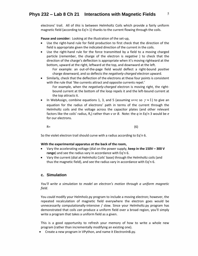
electrons’ trail. All of this is between Helmholtz Coils which provide a fairly uniform magnetic field (according to Eq’n 1) thanks to the current flowing through the coils.

Pause and consider: Looking at the illustration of the set-up,

Use the right-hand rule for field production to first check that the direction of the field is appropriate given the indicated direction of the current in the coils.

Use the right-hand rule for the force transmitted by a field to a moving charged particle (remember, the charge of the electron is negative ) to check that the direction of the charge’s deflection is appropriate when it’s moving rightward at the bottom, upward at the right, leftward at the top, and downward at the left.

For example: an out-of-the-page field would deflect a right-bound positive charge downward, and so deflects the negatively-charged electron upward.

Similarly, check that the deflection of the electrons at these four points is consistent with the rule that ‘like currents attract and opposite currents repel.’

For example, when the negatively-charged electron is moving right, the right-bound current at the bottom of the loop repels it and the left-bound current at the top attracts it.

In WebAssign, combine equations 1, 3, and 5 (assuming v<<c so 1 ) to give an

equation for the radius of electrons’ path in terms of the current through the Helmholtz coils and the voltage across the capacitor plates (and other relevant factors like the coils’ radius, Rc) rather than v or B. Note: the q in Eq’n 3 would be e for our electrons.

R= (6)

So the violet electron trail should curve with a radius according to Eq’n 6.

With the experimental apparatus at the back of the room,

Vary the accelerating voltage (dial on the power supply, keep in the 150V – 300 V range) and see the radius vary in accordance with Eq’n 6.

Vary the current (dial at Helmholtz Coils’ base) through the Helmholtz coils (and thus the magnetic field), and see the radius vary in accordance with Eq’n 6.

c. Simulation

You’ll write a simulation to model an electron’s motion through a uniform magnetic field. You could modify your Helmholz.py program to include a moving electron; however, the repeated recalculation of magnetic field everywhere the electron goes would be unnecessarily computationally-intensive / slow. Since your Helmholtz.py program has demonstrated that coils can produce a uniform field over a broad region, you’ll simply write a program that takes a uniform field as a given. This is a good opportunity to refresh your memory of how to write a whole new program (rather than incrementally modifying an existing one).

Create a new program in VPython, and name it ElectronInB.py.


What follows will guide you through filling in the sections of the code. Beginning

As with all of your programs, you’ll want to start off with the two from…import… lines (the exact same ones that start your Helmholtz.py program) and follow those with a comment line that includes your names.

Constants

Define:

the magnetic field vector (B) to be 0.0001 Tesla in the +y direction

a variable (Bscale) to scale the size of the arrows representing the magnetic field (start with 500.0)

the time step (dt) to be s 101 10

the maximum time (tmax) to be 1×10-6 s.

Objects

Create a sphere called “electron” to represent an electron by filling in the definition

electron = sphere(...)

with the following attributes

o an initial position (pos) of m 0,0,0 .

o a radius of 5 mm (much larger than its actual size so it can be seen in your simulation).

o a color of color.blue

o a mass of kg 101.9 31

o a charge of C 106.1 19 o an initial velocity of v = vector(0,0,1e6), units of m/s o and set it to leave a trail everywhere it goes by including, along with these other

attributes, “make_trail=true” inside the definition of the electron.

At a few observation locations, create arrows to represent the uniform magnetic field. You can do this however you like, but here’s one way:

d = 0.1 #in meters, coordinates of observation locations

obslocs = [vector(-d,0,-d), vector(-d,0,d), vector(d,0,-d),

vector(d,0,d)] #list of obslocs

for obsloc in obslocs:

arrow(pos = obsloc, axis = B*Bscale,

color = color.cyan)

Initial Values

Initialize the time at t = 0.

Calculations

It’s been a while since you’ve written dynamics programs (ones that simulate the motion of particles in response to forces), so here’s a quick refresher: You have a while loop that steps through time, from t = 0 to some final time, tmax; inside that loop, you recalculate the force on the particle (according to Eq’n 2 in this case), then the particle’s new velocity according to the approximation

tm

Fvv

oldnew ,


and then the particle’s new position according to

tvrr

oldnew .

Of course, you update the time too;

ttt oldnew

I’ll get you started, but you’ll need to complete each line of code

(remember, BA

in Python is cross(A,B)) .

While t < tmax:

F = …

electron.v = …

electron.pos =…

t = …

rate(50000)

Run the program and make sure the electron behaves as you expect.

Pause and consider:

How would you expect the charged particle to behave differently if it had a positive charge instead of a negative charge? Flip the sign of the charge and run the program again.

How would you expect the charged particle to behave differently if it were initially going faster? Double its initial speed and run the program again.

How would you expect the charged particle to behave differently if it initially had a component of velocity parallel to the field (remember, there can be no component of the force parallel to the field)? Give the particle’s velocity an initial y component of 1×104 m/s and run the program again.

Compare with Theory:

Radius. According to Eq’n (3), we expect a specific radius of the particle’s orbit for given mass, speed, charge, and magnetic field. You’ll have the program determine the theoretical and simulated radii.

Theoretical

Just before and outside the while loop, add a line to calculate the expected radius, rtheory, based on the charge, mass, field, and speed (which is mag(electron.v)).

Follow that with the print line

print(“the expected orbital radius is ”, rtheory, “ m.”)

What value do you get?


Simulated

Assuming the electron is indeed executing circular motion in the x-z plane, then the diameter of the orbit would the its maximum z coordinate minus its minimum z coordinate (and the radius would simply be half the diameter). So,

To find the maximum and minimum x coordinates, add following lines

o In the Initialization section, define

Zmax = electron.z

Zmin = electron.z

o At the bottom inside the while loop add

if electron.z > Zmax:

Zmax = electron.z

o Add some similar lines to determine Zmin.

o At the end of the program (outside the while loop), add (and complete) the line

rsimulate = … #the radius of the simulated orbit,

based on Zmin and Zmax

print(“the simulated orbital radius is ”, rsimulate, “ m.”)

Run the program and see how the theoretical and simulated radii compare.

Period

According to Eq’n (4), we expect the period of the electron’s orbit to depend on the field strength, speed, mass, and charge in a specific way.

Theoretical

Before and outside the while loop, add a line to calculate the expected period, Ttheory, based on the charge, mass, and field strength. Then add a print statement to print out this value.

What value do you get?

Simulation

As the particle goes back and forth, the x-component of its velocity flips sign twice per orbit – first switching from heading left to heading right, and then switching from heading right to heading left. So you can determine the period by counting the time between these flips, and doubling it.

In the initialization section, define

Fliptime = 0 #will keep track of when the velocity flips direction

At the top inside the while loop add the line


Oldvx = electron.v.x

At the bottom inside the while loop add the lines

if Oldvx/electron.v.x <0: #true if velocity flipped direction

T = 2*(t – Fliptime)

Fliptime = t

At the bottom of the program, add the print line

print(“the simulated orbital period is ”,T,” s.”)

Run the program and see how the theoretical and simulated periods compare.

When satisfied, save and upload the program.

III. Dipole in a Uniform Magnetic Field

a. Theory A disc magnet is the most readily identifiable magnetic dipole. As the name suggests, a

magnetic “dipole” has two “poles” – North from which magnetic field lines emanate, and

South into which magnetic field lines terminate. (In reality, magnetic field lines are

closed loops that continue on through the body of the magnet). The simplest magnetic

dipole to picture and understand is a single loop of current – charged particles speeding

around in a circle. From Phys 231, you may recall that angular momentum can be

defined for particles moving around in a loop, and that property is useful for discussing

the work and torque required to change the particles’ circular motion. As the angular

momentum focuses on the motion of mass, the magnetic moment focuses on the

corresponding motion of charge. It is similarly useful for discussing the work and torque

associated with the moving charges’ interactions with a magnetic field.

Like angular momentum, the magnetic moment vector’s direction follows from a right-

hand rule: if the current flows counter-clockwise about the y axis, then the magnetic

moment points in the +y direction; if the current flows clockwise about the y axis, then

the magnetic moment points in the – y direction.

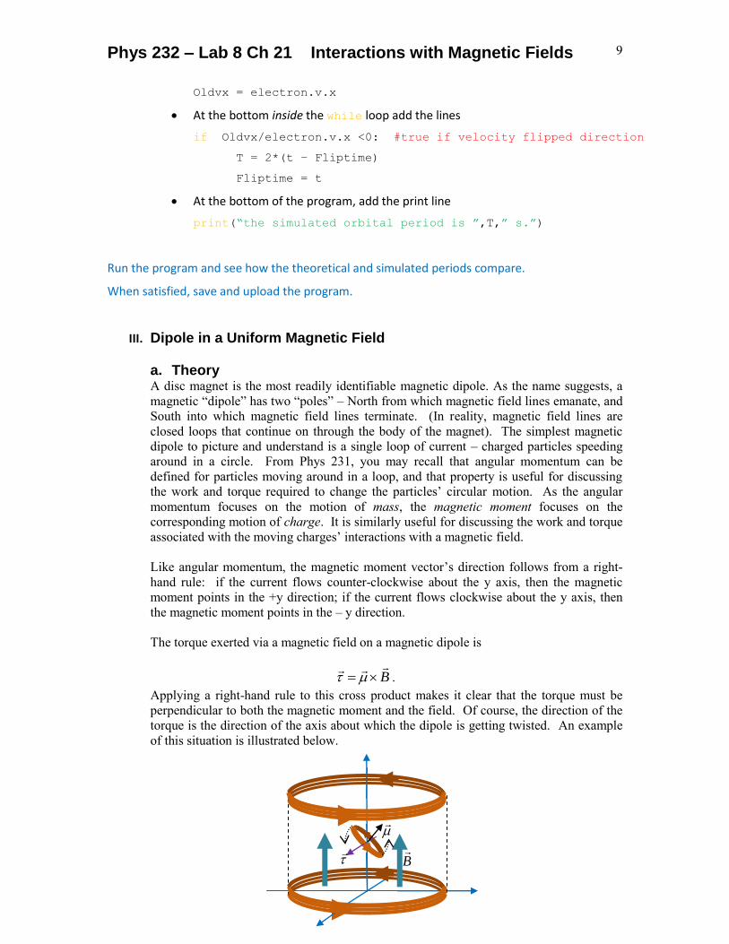
The torque exerted via a magnetic field on a magnetic dipole is

B

.

Applying a right-hand rule to this cross product makes it clear that the torque must be

perpendicular to both the magnetic moment and the field. Of course, the direction of the

torque is the direction of the axis about which the dipole is getting twisted. An example

of this situation is illustrated below.

B


In this example, the magnetic moment of the small coil points up and right while the field

of the large coils points up; accordingly, the torque vector points out of the page,

meaning that the small coils is pushed so its right edge would rise and its left edge would

fall. Though mathematically more complex, a conceptually simpler argument is that the

small coil experiences a torque to bring its current into better alignment with the current

in the large coils because parallel currents attract and anti-parallel currents repel.


Experimental Setup A magnetic dipole (disc magnet) hangs from a spring and is mounted so it can pivot in response to a torque transmitted by a magnetic field. This hangs near the middle of a pair of Helmholtz Coils whose current, and thus field, you can control with the power supply. (It’s for a later experiment that the current is routed through a precision resistor.)

Torque Experiment

Make sure the magnet’s dipole moment points at an angle off vertical (an arrow on its side marks its orientation.) If it isn’t already, you can do this by lifting the plastic cap, (along with rod, spring and dipole) from the graduated cylinder, tipping the dipole, and then replacing the cap (rod, spring, and dipole.)

Turn on the power supply (switch is on the back) and observe the dipole’s response.

Turn off the power supply, unplug the cables form it and re-plug them reversed (red cable to black port and vice versa). This reverses the direction of current flow through the Helmholtz coils, and thus the direction of their magnetic field.

Turn the power supply back on and observe the dipole’s response.

Force Experiment

Dial up the current flowing through the coils, thus the field strength, and observe the dipole’s response. Though the intrinsic current in the dipole (in this case, electrons orbiting their atoms) is attracted to the parallel current flowing through the Helmholtz coils, the attraction to the top coils is the same as that to the bottom coil, so the dipole experiences no net force under the symmetric, constant-field condition.


Interaction with a linearly-Varying Magnetic Field All of the preceding theory, simulations, and experiments have pertained to uniform magnetic fields. Now you’ll explore the simplest non-uniform magnetic field – one that points only along one axis with a strength (and direction) that varies linearly along that direction.

I. Producing a linearly-Varying Magnetic Field

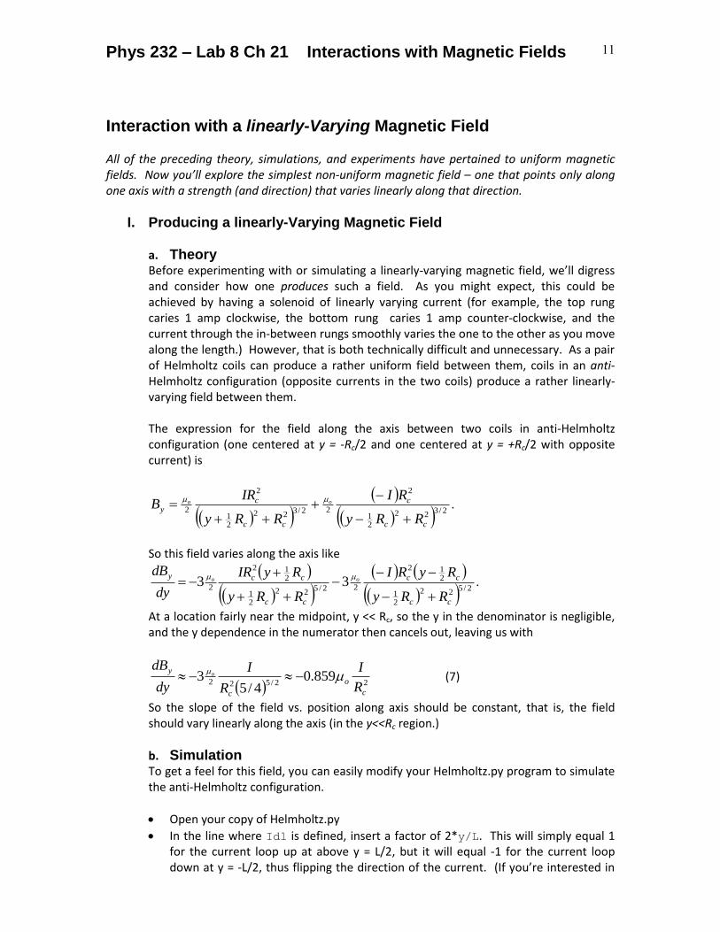
a. Theory Before experimenting with or simulating a linearly-varying magnetic field, we’ll digress and consider how one produces such a field. As you might expect, this could be achieved by having a solenoid of linearly varying current (for example, the top rung caries 1 amp clockwise, the bottom rung caries 1 amp counter-clockwise, and the current through the in-between rungs smoothly varies the one to the other as you move along the length.) However, that is both technically difficult and unnecessary. As a pair of Helmholtz coils can produce a rather uniform field between them, coils in an anti-Helmholtz configuration (opposite currents in the two coils) produce a rather linearly-varying field between them. The expression for the field along the axis between two coils in anti-Helmholtz configuration (one centered at y = -Rc/2 and one centered at y = +Rc/2 with opposite current) is

2/322

21

2

22/322

21

2

2

cc

c

cc

cy

RRy

RI

RRy

IRB oo

.

So this field varies along the axis like

2/522

21

212

22/522

21

212

233

cc

cc

cc

ccy

RRy

RyRI

RRy

RyIR

dy

dBoo

.

At a location fairly near the midpoint, y << Rc, so the y in the denominator is negligible, and the y dependence in the numerator then cancels out, leaving us with

22/522859.0

4/53

c

o

c

y

R

I

R

I

dy

dBo

(7)

So the slope of the field vs. position along axis should be constant, that is, the field should vary linearly along the axis (in the y<<Rc region.)

b. Simulation To get a feel for this field, you can easily modify your Helmholtz.py program to simulate the anti-Helmholtz configuration.

Open your copy of Helmholtz.py

In the line where Idl is defined, insert a factor of 2*y/L. This will simply equal 1 for the current loop up at above y = L/2, but it will equal -1 for the current loop down at y = -L/2, thus flipping the direction of the current. (If you’re interested in


seeing what a linearly-varying solenoid would be like, just increase the number of current loops to something large, like 50.)

Run the program and observe the length of the region over which By varies linearly with y.

II. Dipole Interacting with a Linearly-Varying Magnetic Field

a. Theory Imagine a dipole built of a coil of current-carrying wire, and the coil has non-negligible height. In a regular Helmholtz coil setup, the top loop of this dipole is just as strongly attracted to the current in the upper Helmholtz coil above it as the bottom loop of this dipole is attracted to the lower Helmholtz coil below it, so the dipole experiences no net force. Equivalently, we can relate this to the associated uniform field (rather than directly to the currents that produce it) and say that in the uniform field of the Helmholtz coils, there is no net force on a dipole. You’ve already observed that a dipole will twist but not accelerate and translate due to a uniform field. However, in an anti-Helmholtz setup, if the coil below attracts the dipole, the coil above repels it, so the dipole does feel a net force. Equivalently, we can say that if the field varies along the length of the dipole, then the two faces feel unbalanced forces, and so there is a net force. Mathematically, that is expressed as

BF

,

In our case, the dipole is free to (and will) align with the field that points along the y axis, so we can write more specifically and simply

dy

dBF

y

y . (8)


Experimental Setup This is the same as for the Helmholtz configuration except the power supply is connected so the current flows in the opposite directions in the two coils. Note the different wiring in the diagram.


Experiment

Turn on the power supply and pass a current of about 2 amps.

In the plastic cap, loosen the set screw that holds the brass rod (to which the spring and thus magnet are attached) and raise it enough that the dipole goes above the top coil, then lower it until the dipole is below the midpoint.

What does the dipole do as it crosses below the midpoint?

Pause and consider: Thinking of the field illustrated in your simulation, reason out why the dipole behaves as it does as you lower it. Here’s a start: when the dipole is above the top coil, it’s oriented so that it’s aligned with and attracted to the current in the top ring. As you lower the dipole…

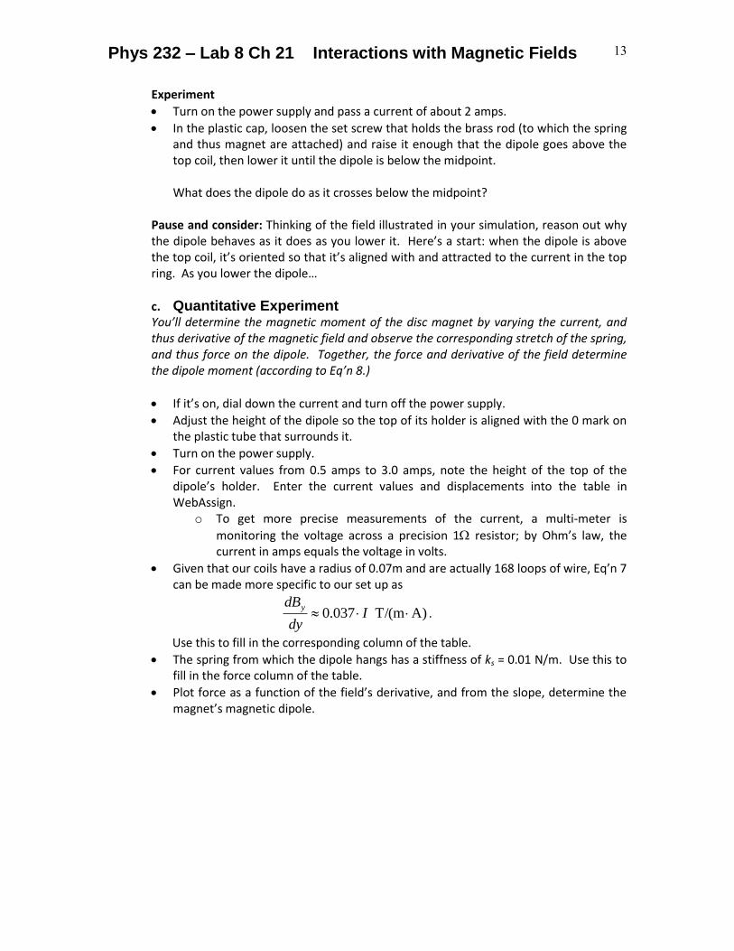
c. Quantitative Experiment You’ll determine the magnetic moment of the disc magnet by varying the current, and thus derivative of the magnetic field and observe the corresponding stretch of the spring, and thus force on the dipole. Together, the force and derivative of the field determine the dipole moment (according to Eq’n 8.)

If it’s on, dial down the current and turn off the power supply.

Adjust the height of the dipole so the top of its holder is aligned with the 0 mark on the plastic tube that surrounds it.

Turn on the power supply.

For current values from 0.5 amps to 3.0 amps, note the height of the top of the dipole’s holder. Enter the current values and displacements into the table in WebAssign.

o To get more precise measurements of the current, a multi-meter is

monitoring the voltage across a precision 1 resistor; by Ohm’s law, the current in amps equals the voltage in volts.

Given that our coils have a radius of 0.07m and are actually 168 loops of wire, Eq’n 7 can be made more specific to our set up as

A)T/(m 037.0 Idy

dBy.

Use this to fill in the corresponding column of the table.

The spring from which the dipole hangs has a stiffness of ks = 0.01 N/m. Use this to fill in the force column of the table.

Plot force as a function of the field’s derivative, and from the slope, determine the magnet’s magnetic dipole.


Helmholtz.py


ElectronInB.py

The modification to Helmholtz.py to make it antiHelmholt.py

phys 232 lab 8 ch 21 interactions with magnetic...

Documents