phy331: advanced electrodynamics & magnetism electrodynamics, and it has everything that is...
TRANSCRIPT
PHY331: Advanced Electrodynamics & Magnetism
Part I: Electrodynamics
Contents
1 Field theories and vector calculus 31.1 Field theory . . . . . . . . . . . . . . . . . . . . . . . . . . . . . . . . . . . . 31.2 Vector calculus . . . . . . . . . . . . . . . . . . . . . . . . . . . . . . . . . . . 41.3 Second derivatives . . . . . . . . . . . . . . . . . . . . . . . . . . . . . . . . 71.4 Tensors . . . . . . . . . . . . . . . . . . . . . . . . . . . . . . . . . . . . . . . 81.5 Index notation . . . . . . . . . . . . . . . . . . . . . . . . . . . . . . . . . . . 10
2 Electromagnetic forces, potentials, Maxwell’s equations 132.1 Electrostatic forces and potentials . . . . . . . . . . . . . . . . . . . . . . . . 132.2 Magnetostatic forces . . . . . . . . . . . . . . . . . . . . . . . . . . . . . . . 142.3 Electrodynamics and Maxwell’s equations . . . . . . . . . . . . . . . . . . . 162.4 Charge conservation . . . . . . . . . . . . . . . . . . . . . . . . . . . . . . . 162.5 The vector potential . . . . . . . . . . . . . . . . . . . . . . . . . . . . . . . . 17
3 Electrodynamics with scalar and vector potentials 213.1 Scalar and vector potential . . . . . . . . . . . . . . . . . . . . . . . . . . . . 213.2 Gauge transformations . . . . . . . . . . . . . . . . . . . . . . . . . . . . . . 213.3 A particle in an electromagnetic field . . . . . . . . . . . . . . . . . . . . . . 22
4 Electromagnetic waves and Poynting’s theorem 254.1 Electromagnetic waves . . . . . . . . . . . . . . . . . . . . . . . . . . . . . . 254.2 Complex fields? . . . . . . . . . . . . . . . . . . . . . . . . . . . . . . . . . . . 264.3 Poynting’s theorem . . . . . . . . . . . . . . . . . . . . . . . . . . . . . . . . 27
5 Momentum of the electromagnetic field 31
6 Multipole expansion and spherical harmonics 346.1 Multipole expansion of a charge density . . . . . . . . . . . . . . . . . . . . 346.2 Spherical harmonics and Legendre polynomials . . . . . . . . . . . . . . . 366.3 Multipole expansion of a current density . . . . . . . . . . . . . . . . . . . 37
7 Dipole fields and radiation 417.1 Electric dipole radiation . . . . . . . . . . . . . . . . . . . . . . . . . . . . . 417.2 Magnetic dipole radiation . . . . . . . . . . . . . . . . . . . . . . . . . . . . 437.3 Larmor’s formula . . . . . . . . . . . . . . . . . . . . . . . . . . . . . . . . . 43
PHY331 PART I: ADVANCED ELECTRODYNAMICS LECTURE 0
8 Electrodynamics in macroscopic media 478.1 Macroscopic Maxwell equations . . . . . . . . . . . . . . . . . . . . . . . . 478.2 Polarization and Displacement fields . . . . . . . . . . . . . . . . . . . . . . 478.3 Magnetization and Magnetic induction . . . . . . . . . . . . . . . . . . . . 49
9 Waves in dielectric and conducting media 529.1 Waves in dielectric media . . . . . . . . . . . . . . . . . . . . . . . . . . . . 529.2 Waves in conducting media . . . . . . . . . . . . . . . . . . . . . . . . . . . 559.3 Waves in plasmas . . . . . . . . . . . . . . . . . . . . . . . . . . . . . . . . . 57
10 Relativistic formulation of electrodynamics 5910.1 Four-vectors and transformations in Minkowski space . . . . . . . . . . . . 5910.2 Covariant Maxwell equations . . . . . . . . . . . . . . . . . . . . . . . . . . 6210.3 Invariant quantities . . . . . . . . . . . . . . . . . . . . . . . . . . . . . . . . 65
A Special coordinates and vector identities 67A.1 Coordinate systems . . . . . . . . . . . . . . . . . . . . . . . . . . . . . . . . 67A.2 Integral theorems and vector identities . . . . . . . . . . . . . . . . . . . . . 69A.3 Levi-Civita tensor . . . . . . . . . . . . . . . . . . . . . . . . . . . . . . . . . 69
B Unit systems in electrodynamics 70
Literature
The lecture notes are intended to be mostly self-sufficient, but below is a list of recom-mended books for this course:
1. R.H. Good, Classical Electromagnetism, Saunders College Publishing (1999). Mostof the material in this course is covered in this book. It is very accessible andprobably should be your first choice to look something up.
2. J.D. Jackson, Classical Electrodynamics, Wiley (1998). This is the standard work onclassical electrodynamics, and it has everything that is covered in this course. Thelevel is quite high, but it will answer your questions.
3. R.P. Feynman, Lectures on Physics, Addison-Wesley (1964). Probably the best gen-eral books on physics ever. The emphasis is on the physical intuition, and it iswritten in a very accessible narrative.
4. J. Schwinger et al., Classical Electrodynamics, Westview Press (1998). This is quite ahigh-level textbook, containing many topics. It has detailed mathematical deriva-tions of nearly everything.
After each lecture there is a detailed “further reading” section that points you to therelevant chapters in various books.
2
PHY331 PART I: ADVANCED ELECTRODYNAMICS LECTURE 1
1 Field theories and vector calculus
1.1 Field theory
Michael Faraday(1791-1867)
Electrodynamics is a theory of fields, and all matter entersthe theory in the form of densities. All modern physicaltheories are field theories, from general relativity to thequantum fields in the standard model and string theory.Therefore, apart from learning some important topics inelectromagnetism, in this course you will aquire an under-standing of modern field theories without having to dealwith the strangeness of quantum mechanics or the math-ematical difficulty of general relativity. Fields were intro-duced by Michael Faraday, who came up with “lines offorce” to describe magnetic phenomena.You will be familliar with particle theories such as clas-
sical mechanics, where the fundamental object is char-acterised by a position vector and a momentum vector.Ignoring the possible internal structure of the particles,they have six degrees of freedom (three position and threemomentum components). Fields, on the other hand, arecharacterised by an infinite number of degrees of freedom.Let’s look at some examples:A vibrating string: Every point x along the string has a displacement r, which is adegree of freedom. Since there are an infinite number of points along the string, thedisplacement r(x) is a field. The argument x denotes a location on a line, so we call thefield one-dimensional.Landscape altitude: With every point on a surface (x, y), we can associate a numberthat denotes the altitude h. The altitude h(x, y) is a two-dimensional field. Since thealtitude is a scalar, we call this a scalar field.Temperature in a volume: At every point (x, y, z) in the volume we can measure thetemperature T, which gives rise to the three-dimensional scalar field T(x, y, z).Mathematically, we denote a field by F(r, t), where the value of the field at position
r and time t is given by the quantity F. This quantity can be anything: if F is a scalar, wespeak of a scalar field, and if F is a vector we speak of a vector field. In quantum fieldtheory, the mathematical object that makes the quantum field are operators acting on avacuum state.In this course we will be mostly dealing with scalar and vector fields, but occasion-
ally we will encounter tensor fields. A common example of a tensor field that you mayhave encountered is the stress in a material. We will discuss the difference betweentensors and ordinary matrices in a moment.
3
PHY331 PART I: ADVANCED ELECTRODYNAMICS LECTURE 1
1.2 Vector calculus
In mechanics, a particle does not randomly jump around in phase space, but followsequations of motion determined by the laws of mechanics and the boundary conditions.These equations of motion typically involve derivatives, namely the velocity and accel-eration of the particle. The derivatives tell you howmuch a quantity changes. Likewise,fields obey equations of motion, and we need to define the derivatives of fields.First, take the scalar field. The interesting aspect of such a field is how the values of
the field change when we move to neighbouring points in space, and in what directionthis change is maximal. For example, in the altitude field (with constant gravity) thischange determines how a ball would roll on the surface, and for the temperature fieldit determines how the heat flows.It is easy to see that both a rolling ball and heat flow have a magnitude and a direc-
tion. The measure of change of a scalar must therefore be a vector. Since the change isdefined at every point r (and time t), it is a vector field. Let the scalar field be denoted byf (x, y, z, t). Then the change in the x direction (denoted by i) is given by
limh→0f (x+ h, y, z, t) − f (x, y, z, t)
hi =
∂ f (x, y, z, t)∂x
i . (1.1)
Ax(r+ l i)
Ax(r)
Ay(r) Ay
Az(r)
Az(r+ l k)
l
ll
r
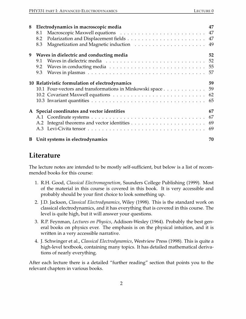
Figure 1: The divergence of a vector field Acan be found by considering the total flux ofA through the faces of a small cube of volumel3 at point r = x i+ y j+ z k.
Similar expressions hold for the change inthe y and z direction, and in general the spa-tial change of a scalar field is given by
∂ f∂xi+
∂ f∂yj+
∂ f∂zk = ∇ f ≡ grad f , (1.2)
called the gradient of f . The “nabla” or “del”symbol ∇ is a differential operator, and it isalso a vector:
∇ = i∂
∂x+ j
∂∂y
+ k∂∂z. (1.3)
Clearly, this makes a vector field out of ascalar field. Note that we do not includechanges over time in the gradient. We firststudy static fields.When we want to describe the behaviour
of vector fields, there are twomain concepts:the divergence and the curl. The divergence isa measure of flow into, or out of, a volumeelement. Consider a volume element dV =
l3 at point r = x i + y j + z k and a vector field A(x, y, z), as shown in figure 1. Weassume that l is very small. The difference of the flux of the field going into the volume
4

PHY331 PART I: ADVANCED ELECTRODYNAMICS LECTURE 1
A(x− l, y− l) A(x+ l, y− l)
A(x+ l, y+ l) A(x− l, y+ l)
y
xx− l x+ l
y− l
y+ l
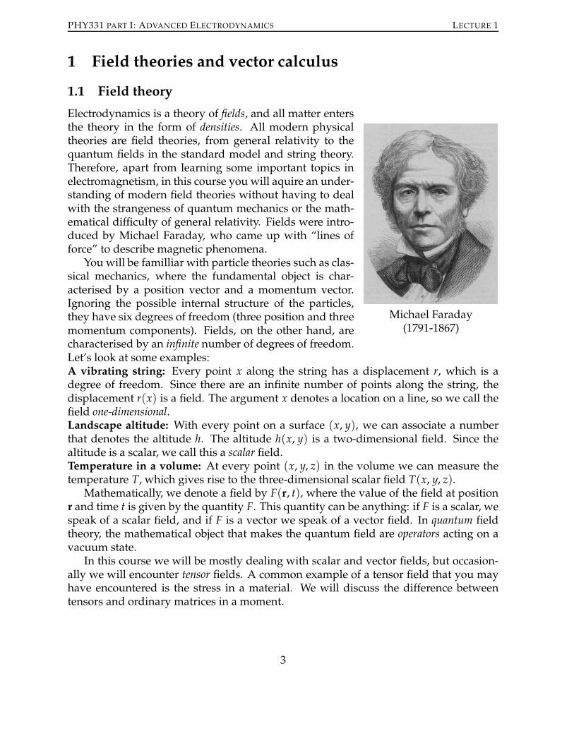
Figure 2: The curl of a vector field A can be found by considering the change of the vector fieldaround a closed loop.
and the flux coming out of the volume in the x direction l2Ax(r+ l i)− l2Ax(r) is relatedto the change of the component Ax in the x direction. From the Taylor expansion we getthe approximation (l ≪ 1, and ultimately infinitesimal)
Ax(x+ l, y) = Ax(x, y) + l∂Ax∂x
(x, y) . (1.4)
This leads to
l2Ax(x+ l, y, z) − l2Ax(x, y, z) = l3∂Ax∂x.
In order to find the total change in the vector field we have to add the changes in the yand z components as well, which then leads to
∂Ax∂x
+∂Ay∂y
+∂Az∂z
= ∇ ·A ≡ divA , (1.5)
where we removed the common factor l3 in order to consider the divergence per unitvolume. By taking l infinitesimally small, we can properly define the divergence (andlater the curl) at a single point. The divergence is a measure of how the vector fieldA(r)spreads out at position r.The curl of a vector field is a measure of the vorticity of the field. In two dimensions
(here meaning the xy plane), consider a four-part infinitesimal closed loop starting atpoint (x − l, y − l), going to (x + l, y − l), (x + l, y + l) and via (x − l, y + l) back to(x − l, y − l), as shown in figure 2. The area of the square is 4l2. The accumulatedchange of the vector field around this loop is given by the projection of A along the lineelements. We evaluate all four sides of the infinitesimal loop in Fig. 2. For example, theline element that stretches from x− l to x+ l at y− l is oriented in the x direction, andthe corresponding A · dl is
(
Ax i+ Ay j+ Az k)
·(
2l i+ 0 j+ 0 k)
= 2lAx(x, y− l) , (1.6)
5

PHY331 PART I: ADVANCED ELECTRODYNAMICS LECTURE 1
where we evaluate Ax in the middle of the line element at the point (x, y− l). We repeatthe same procedure for the other three line elements. Make sure you get the orientationright, because the top horizontal part is directed in the−x direction. The correspondingterm gets a minus sign. Now add them all up and get A · dl around the loop:
∮
A · dl = 2lAx(x, y− l) + 2lAy(x+ l, y) − 2lAx(x, y+ l)− 2lAy(x− l, y) . (1.7)
Just like for the divergence, we can use the first two terms in Taylor’s expansion ofA j(x+ l, y) to evaluate this formally, since l will be again an infinitesimal length. Forexample:
Ax(x, y+ l) = Ax(x, y) + l∂Ax∂y
(x, y) . (1.8)
This leads to∮
A · dl = 4l2(
∂Ay∂x
− ∂Ax∂y
)
. (1.9)
For a three-dimensional vector space, we not only have to take the contribution of a loopin the xy plane, but also in the xz and the yz planes. Since there are three orthogonalloops, they can be thought of as the components of a vector. For a three-dimensionalvector field we thus have
i
(
∂Az∂y
− ∂Ay∂z
)
+ j
(
∂Ax∂z
− ∂Az∂x
)
+ k
(
∂Ay∂x
− ∂Ax∂y
)
= ∇×A ≡ curlA , (1.10)
the curl of a vector field A per unit surface 4l2. We again take l → 0 to define the curl ofA(r) at a point r.In four dimensions (which is relevant when we do relativity) we have loops not only
in the xy, xz, and yz planes, but also in the xt, yt, and zt planes. As you can see, there arenow six loops, which can no longer be regarded as components of a three-dimensionalvector. Therefore the cross product (and hence the curl operator) as a vector is specialto three-dimensional space.In compact matrix notation, the curl can be written as a determinant
∇×A =
∣
∣
∣
∣
∣
∣
i j k∂x ∂y ∂zAx Ay Az
∣
∣
∣
∣
∣
∣
. (1.11)
Sometimes, when there are a lot of partial derivatives in an expression or derivation, itsaves ink and space to write the derivative ∂/∂x as ∂x, etc.The curl and the divergence are in some sense complementary: the divergence mea-
sures the rate of change of a field along the direction of the field, while the curl measuresthe behaviour of the transverse field. If both the curl and the divergence of a vector fieldA are known, andwe also fix the boundary conditions, then this determinesA uniquely.
6
PHY331 PART I: ADVANCED ELECTRODYNAMICS LECTURE 1
It seems extraordinary that you can determine a field (which has after all an infinitenumber of degrees of freedom) with only a couple of equations, so let’s prove it. Sup-pose that we have two vector fields A and B with identical curls and divergences, andthe same boundary conditions (for example, the field is zero at infinity). We will showthat a third field C = A−Bmust be zero, leading to A = B. First of all, we observe that
∇×C = ∇×A−∇×B = 0∇ · C = ∇ ·A−∇ · B = 0 , (1.12)
so C has zero curl and divergence. We can use a vector identity (see Appendix A) toshow that the second derivative of C is also zero:
∇2C = ∇(∇ · C)−∇×(∇×C) = 0− 0 = 0 . (1.13)
This also means that the Laplacian ∇2 of every independent component of C is zero.Since the boundary conditions for A and B are the same, the boundary conditions forC must be zero. So with all that, can C be anything other than zero? Eq. (1.13) does notpermit any local minima or maxima, and it must be zero at the boundary. Therefore,it has to be zero inside the boundary as well. This proves that C = 0, or A = B.Therefore, by determining the divergence and curl, the vector field is completely fixed,up to boundary conditions.Looking ahead at the next lecture, you now know why there are four Maxwell’s
equations: two divergences and two curls for the electric and magnetic fields (plus theirtime derivatives). These four equations and the boundary conditions completely deter-mine the fields, as they should.
1.3 Second derivatives
In physics, many properties depend on second derivatives. The most important exam-ple is Newton’s second law F = ma, where a is the acceleration, or the second derivativeof the position of a particle. It is therefore likely that we are going to encounter the sec-ond derivatives of fields as well. In fact, we are going to encounter them a lot! So whatcombinations can we make with the gradient, the divergence, and the curl?The div and the curl act only on vectors, while the grad acts only on scalars. More-
over, the div produces a scalar, while the grad and the curl produce vectors. If f isa scalar field and A is a vector field, you can convince yourself that the six possiblecombinations are
∇ · (∇ f ) ∇(∇ ·A) ∇×(∇ f )
∇ · (∇×A) ∇×(∇×A) ∇2A
Of these, the first (∇ · (∇ f )) and the last (∇2A) are essentially the same, since in thelatter case the Laplacian acts on each component of A independently, and a componentof a vector is a scalar.
7

PHY331 PART I: ADVANCED ELECTRODYNAMICS LECTURE 1
Another simplification is that two of the six expressions above are identically zerofor any f or A:
∇ · (∇×A) = 0 and ∇×(∇ f ) = 0 . (1.14)
Since these identities tend to simplify equations a lot, it is a good idea to learn them byheart. The remaining derivatives are related by the vector identity
∇×(∇×A) = ∇(∇ ·A)−∇2A , (1.15)
which is also used very often. In fact, we just used it in Eq. (1.13). All these relations,and more, can be found in Appendix A.
1.4 Tensors
Let’s talk about vectors and tensors. You know that a vector is a quantity with a mag-nitude and a direction. There is, however, also a more formal definition, which makesit easier to generalise the concept of a vector to higher rank objects such as matrices (re-member, a scalar has rank 0, a vector has rank 1, a matrix has rank 2, etc.). These objectsare called tensors. A tensor of rank 0 is just a scalar, and a tensor of rank 1 is just a vector.A tensor of rank 2 is indeed a matrix, but is every matrix a tensor of rank 2? The answeris no, because tensors must obey certain transformation properties. The formal definitionof a tensor says that it is an object that transforms in a special way under coordinatetransformations. To see what we mean by this, consider again the case of a vector.We can write a vector ~a in Cartesian coordinates as a list of components (ax , ay , az)
or, in our notation, ax i + ay j + az k. But the coordinate system is something that wechoose, and has nothing to do with the vector itself. In particular, we can rotate ourcoordinates around the z axis over an angle θ according to
x′ = cosθ x+ sinθ yy′ = − sinθ x+ cosθ yz′ = z . (1.16)
Since the vector ~a does not change, its description in the new coordinate system mustchange, so
~a = (ax , ay , az) = (cosθ a′x − sinθ a′y, sinθ a′x + cosθ a′y, a′z) . (1.17)
You can view this geometrically as follows: If we rotate our coordinate system overan angle θ, then in the new coordinate system we must rotate the vector back over anangle −θ in order to describe the same vector. This means that you cannot choose anyold function of x, y and z as your vector field, because it must obey this transformationrule. If a j = f (x, y, z), then a′j = f (x′, y′, z′), that is, the same function f . For example,you can check using Eq. (1.16) that A = (y, x, 0) is not a proper vector field.
8
PHY331 PART I: ADVANCED ELECTRODYNAMICS LECTURE 1
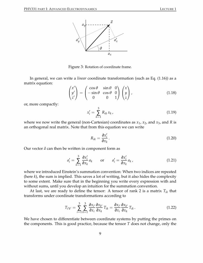
~a
ax
a′x
ay
a′y
θ
Figure 3: Rotation of coordinate frame.
In general, we can write a linear coordinate transformation (such as Eq. (1.16)) as amatrix equation:
x′
y′
z′
=
cosθ sinθ 0− sinθ cosθ 00 0 1
xyz
, (1.18)
or, more compactly:
x′i =3
∑k=1
Rik xk , (1.19)
where we now write the general (non-Cartesian) coordinates as x1, x2, and x3, and R isan orthogonal real matrix. Note that from this equation we can write
Rik =∂x′i∂xk. (1.20)
Our vector~a can then be written in component form as
a′i =3
∑k=1
∂x′i∂xkak or a′i =
∂x′i∂xkak , (1.21)
where we introduced Einstein’s summation convention: When two indices are repeated(here k), the sum is implied. This saves a lot of writing, but it also hides the complexityto some extent. Make sure that in the beginning you write every expression with andwithout sums, until you develop an intuition for the summation convention.At last, we are ready to define the tensor: A tensor of rank 2 is a matrix Tik that
transforms under coordinate transformations according to
Ti′k′ =3
∑i=1
3
∑k=1
∂xi′∂xi
∂xk′∂xkTik =
∂xi′∂xi
∂xk′∂xkTik . (1.22)
We have chosen to differentiate between coordinate systems by putting the primes onthe components. This is good practice, because the tensor T does not change, only the
9
PHY331 PART I: ADVANCED ELECTRODYNAMICS LECTURE 1
coordinate systems change. A general tensor of rank n then obeys
Ti′1 ...i′n=
∂xi′1∂xi1. . .
∂xi′n∂xinTi1 ...in . (1.23)
This includes the regular vector in Eq. (1.21).We will not make use of tensors very often in this course, but they are indispensible
when talking about the momentum of the electromagnetic field, and when we give therelativistic description of Maxwell’s equations. You should therefore be aware that atensor exists, and that it is different from a matrix in its transformation properties.
1.5 Index notation
It is instructive to see how we can write the gradient, the divergence, and the curl inindex notation (using the summation convention). The gradient produces a vector, sowe can write this as
(∇ f )i = (grad f )i = ∂i f . (1.24)
Note that the ith component of the field is given by the derivative ∂i, as it should. Thedivergence is written as
∇ ·A = divA = ∂iAi , (1.25)
where divA does not carry an index because it is a scalar. The repeated index i on theright hand side is summed over, so it does not show up on the left hand side. The curl,finally, makes use of the Levi-Civita tensor ǫi jk, which returns 1 if the sequence i jk is aneven permutation of the index numbers 1, 2, and 3, and it returns −1 if the sequence i jkis an odd permutation of 1, 2, and 3. When some indices are repeated (say i = j), thenthe Levi-Civita tensor returns 0. Verify that the curl of a vector field can be written as
(∇×A)i = (curlA)i = ǫi jk∂ jAk . (1.26)
You can always do an immediate check on equations like this, because the unpairedindices on the left must match the unpaired indices on the right.
Further reading
– D. Mowbray,Mathematics for Electromagnetism, PHY205(http://www.david-mowbray.staff.shef.ac.uk/mathematics for electromagnetism.htm).
– H.M. Schey, Div, Grad, Curl, and all that, Norton & Co. (1973).
– G. Weinreich, Geometrical Vectors, Chicago Lectures in Physics (1998): An unorthodox butvery insightful treatment of vector calculus.
– R.H. Good, Classical Electromagnetism, Saunders College Pub. (1999): Ch. 1, pp 1-32.
– R.P. Feynman, Lectures on Physics, volume II, Addison-Wesley (1964): Ch. 2.
– W.J. Duffin, Electricity and Magnetism, McGraw-Hill (1990): App. A & B, pp 390-405.
10

PHY331 PART I: ADVANCED ELECTRODYNAMICS LECTURE 1
– B.I. Bleaney & B. Bleaney, Electricity and magnetism, Vol. 1, Oxford University Press (1976):App. A, pp A1-A12.
– J.R. Reitz, F.J. Milford, & R.W. Christy, Foundations of Electromagnetic Theory, fourth edition,Addison-Wesley (1993): Ch. 1, pp 1-25.
Exercises
1. Let f = 1√x2+y2+z2
. Calculate
(a) ∇ f ,(b) ∇ ·∇ f .
2. Let A = 12B(−y, x, 0).
(a) Calculate B = ∇×A,(b) Sketch A and B.
3. Prove that ∇ · (∇×A) = 0 and∇×(∇ f ) = 0.
4. LetQ = (−y, x, 0). Can you find a function T such thatQ = ∇T? If T is supposedto be a temperature field, what doesQ represent? Interpret your result physically.
5. Calculate∫
SA · dS, where S is the surface of the unit sphere centered around theorigin, and A is (Hint: use Gauss’ theorem):
(a) A = (−y, x, 0),(b) A = 1
3(x, y, z).
6. Calculate∮
CA · dl, where the closed loop C is the unit circle centered at the ori-gin in the xy plane. It is traversed in anti-clockwise direction (Hint: use Stokes’theorem):
(a) A = (−y, x, 0),(b) A = 1
3(x, y, z).
7. Using arrows of the proper magnitude, sketch
(a) (x, y)
(b) (1, 1)/√2
(c) (0, x)
(d) (y√x2+y2
, x√x2+y2
)
11
PHY331 PART I: ADVANCED ELECTRODYNAMICS LECTURE 1
8. An object moves in the xy plane such that its position at time t is
r = (a cosωt, b sinωt)
with a, b, andω constants.
(a) How far is the object from the origin at time t?
(b) Find the velocity and the acceleration as a function of time.
(c) Show that the object moves in an elliptical path
(x
a
)2+( y
b
)2= 1
9. Find a unit vector normal to each of the following surfaces
(a) z = 2− x− y(b) z = x2 + y2
(c) z =√1− x2
10. Calculate the divergence of F(x, y, z) = ( f (x), f (y), f (−2z)) and show that it be-comes zero at the point (c, c,−c/2).
11. Let F(r) = r f (r) and r = (x, y, z)/r. Determine f (r) such that divF = 0.
12. Calculate the curl of the following functions:
(a) (z2 , x2,−y2)(b) (3xz, 0,−x2)(c) (e−y, e−z, e−x)
(d) (yz, xz, xy)
(e) (−yz, xz, 0)(f) (x, y, x2 + y2)
13. Show that curl 12A×r = A for r = (x, y, z) and A constant.
14. Verify Stokes’ theorem when F = (z2 ,−y2, 0), the closed loop C is given by thesquare (0, 0, 0) → (0, 0, 1) → (1, 0, 1) → (1, 0, 0) → (0, 0, 0), and S is the surfaceof unit cube between (0, 0, 0) and (1, 1, 1) without the side enclosed by C.
15. Verify the vector identities for the first and second derivatives. Use index notation.
12
PHY331 PART I: ADVANCED ELECTRODYNAMICS LECTURE 2
++
(a) (b)
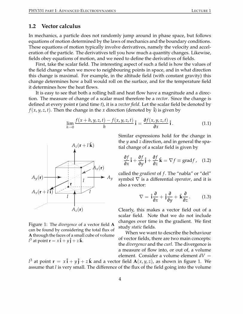
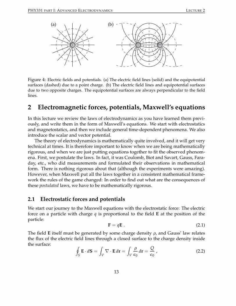
Figure 4: Electric fields and potentials. (a) The electric field lines (solid) and the equipotentialsurfaces (dashed) due to a point charge. (b) The electric field lines and equipotential surfacesdue to two opposite charges. The equipotential surfaces are always perpendicular to the fieldlines.
2 Electromagnetic forces, potentials, Maxwell’s equations
In this lecture we review the laws of electrodynamics as you have learned them previ-ously, and write them in the form of Maxwell’s equations. We start with electrostaticsand magnetostatics, and then we include general time-dependent phenomena. We alsointroduce the scalar and vector potential.The theory of electrodynamics is mathematically quite involved, and it will get very
technical at times. It is therefore important to know when we are being mathematicallyrigorous, and when we are just putting equations together to fit the observed phenom-ena. First, we postulate the laws. In fact, it was Coulomb, Biot and Savart, Gauss, Fara-day, etc., who did measurements and formulated their observations in mathematicalform. There is nothing rigorous about that (although the experiments were amazing).However, when Maxwell put all the laws together in a consistent mathematical frame-work the rules of the game changed: In order to find out what are the consequences ofthese postulated laws, we have to be mathematically rigorous.
2.1 Electrostatic forces and potentials
We start our journey to the Maxwell equations with the electrostatic force: The electricforce on a particle with charge q is proportional to the field E at the position of theparticle:
F = qE . (2.1)
The field E itself must be generated by some charge density ρ, and Gauss’ law relatesthe flux of the electric field lines through a closed surface to the charge density insidethe surface:
∮
SE · dS =
∫
V∇ · E dr =
∫
V
ρ
ǫ0dr =
Q
ǫ0, (2.2)
13
PHY331 PART I: ADVANCED ELECTRODYNAMICS LECTURE 2
(a) (b) (c)
dl I
I
θ
rr B
B
D
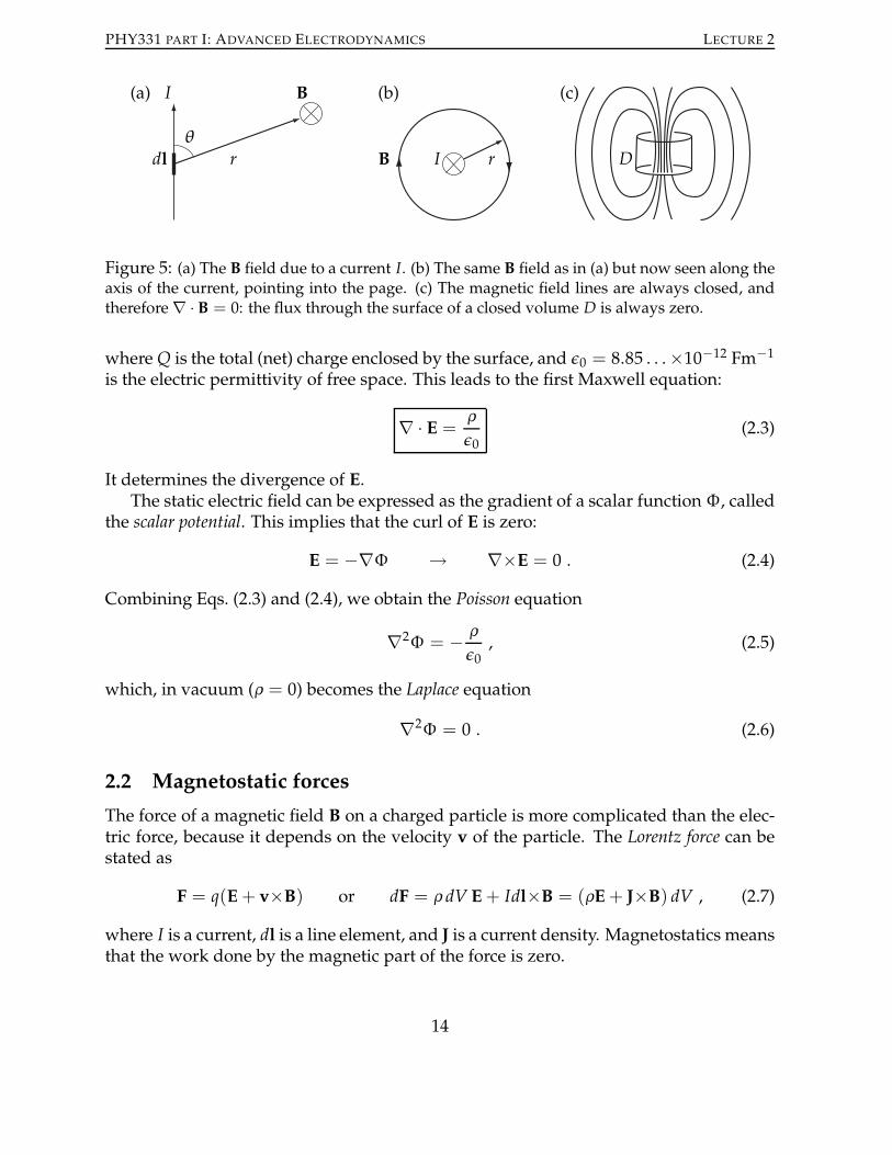
Figure 5: (a) The B field due to a current I. (b) The same B field as in (a) but now seen along theaxis of the current, pointing into the page. (c) The magnetic field lines are always closed, andtherefore∇ · B = 0: the flux through the surface of a closed volume D is always zero.
where Q is the total (net) charge enclosed by the surface, andǫ0 = 8.85 . . .×10−12 Fm−1
is the electric permittivity of free space. This leads to the first Maxwell equation:
∇ · E =ρ
ǫ0(2.3)
It determines the divergence of E.The static electric field can be expressed as the gradient of a scalar function Φ, called
the scalar potential. This implies that the curl of E is zero:
E = −∇Φ → ∇×E = 0 . (2.4)
Combining Eqs. (2.3) and (2.4), we obtain the Poisson equation
∇2Φ = − ρ
ǫ0, (2.5)
which, in vacuum (ρ = 0) becomes the Laplace equation
∇2Φ = 0 . (2.6)
2.2 Magnetostatic forces
The force of a magnetic field B on a charged particle is more complicated than the elec-tric force, because it depends on the velocity v of the particle. The Lorentz force can bestated as
F = q(E+ v×B) or dF = ρ dV E+ Idl×B = (ρE+ J×B) dV , (2.7)
where I is a current, dl is a line element, and J is a current density. Magnetostatics meansthat the work done by the magnetic part of the force is zero.
14
PHY331 PART I: ADVANCED ELECTRODYNAMICS LECTURE 2
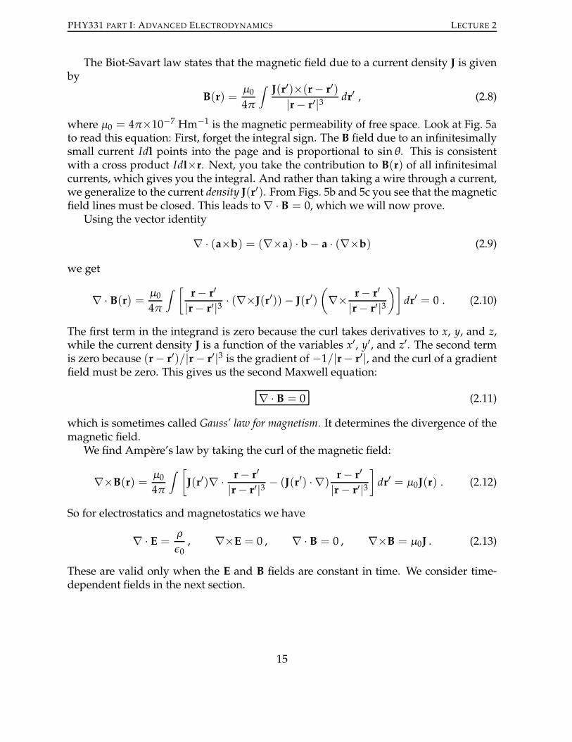
The Biot-Savart law states that the magnetic field due to a current density J is givenby
B(r) =µ0
4π
∫
J(r′)×(r− r′)|r− r′|3 dr′ , (2.8)
where µ0 = 4π×10−7 Hm−1 is the magnetic permeability of free space. Look at Fig. 5ato read this equation: First, forget the integral sign. The B field due to an infinitesimallysmall current Idl points into the page and is proportional to sinθ. This is consistentwith a cross product Idl×r. Next, you take the contribution to B(r) of all infinitesimalcurrents, which gives you the integral. And rather than taking a wire through a current,we generalize to the current density J(r′). From Figs. 5b and 5c you see that the magneticfield lines must be closed. This leads to ∇ · B = 0, which we will now prove.Using the vector identity
∇ · (a×b) = (∇×a) · b− a · (∇×b) (2.9)
we get
∇ · B(r) =µ0
4π
∫
[
r− r′|r− r′|3 · (∇×J(r′)) − J(r′)
(
∇× r− r′|r− r′|3
)]
dr′ = 0 . (2.10)
The first term in the integrand is zero because the curl takes derivatives to x, y, and z,while the current density J is a function of the variables x′, y′, and z′. The second termis zero because (r− r′)/|r− r′|3 is the gradient of −1/|r− r′|, and the curl of a gradientfield must be zero. This gives us the second Maxwell equation:
∇ · B = 0 (2.11)
which is sometimes called Gauss’ law for magnetism. It determines the divergence of themagnetic field.We find Ampere’s law by taking the curl of the magnetic field:
∇×B(r) =µ0
4π
∫
[
J(r′)∇ · r− r′
|r− r′|3 − (J(r′) · ∇)r− r′
|r− r′|3]
dr′ = µ0J(r) . (2.12)
So for electrostatics and magnetostatics we have
∇ · E =ρ
ǫ0, ∇×E = 0 , ∇ · B = 0 , ∇×B = µ0J . (2.13)
These are valid only when the E and B fields are constant in time. We consider time-dependent fields in the next section.
15

PHY331 PART I: ADVANCED ELECTRODYNAMICS LECTURE 2
2.3 Electrodynamics and Maxwell’s equations
C
ΦBI
Figure 6: Lenz’ law.
So far we have considered only electric and magnetic fieldsthat do not change in time. Now, let’s consider general elec-tromagnetic fields. Lenz’ law states that the electromotiveforce E on a closed wire C is related to the change of the mag-netic flux ΦB through the loop:
E =∮
CE · dl = −dΦB
dtand ΦB =
∫
SB(r, t) · dS . (2.14)
Do not confuse ΦB with the scalar potential Φ: they are twocompletely different things! In general, we can define thegeneral (motional) electromotive force as
E =∮
C
F · dlq
=∮
CE · dl+
∮
Cv×B · dl , (2.15)
which has both a purely electric component, as well as a magnetic component due tov×B. This is the motional e.m.f.For a strictly electric e.m.f., we can use Stokes’ theorem to write
∮
CE · dl =
∫
S(∇×E) · dS = −
∫
S
∂B(r, t)
∂t· dS , (2.16)
or
∇×E+∂B(r, t)
∂t= 0 (2.17)
This is Faraday’s law, and our third Maxwell equation.
2.4 Charge conservation
Charges and currents inside a volume V bounded by the surface S can be a function oftime:
Q(t) =∫
Vρ(r, t) dr and I(t) =
∮
SJ · dS =
∫
∇ · J dr . (2.18)
Conservation of charge then tells us that the change of the charge in V is related to theflow of charge through S:
dQ(t)
dt+ I(t) = 0 or
∂ρ
∂t+ ∇ · J = 0 . (2.19)
As far as we know today, charge conservation is strictly true in Nature.
16

PHY331 PART I: ADVANCED ELECTRODYNAMICS LECTURE 2
The fourth, and last, Maxwell equation is a modification of Ampere’s law ∇×B =µ0J. As it turns out, Ampere’s law, as stated in Eq. (2.12) was wrong! Or at least, it doesnot have general applicability. To see this, let’s take the divergence of Eq. (2.12):
∇ · J =1
µ0∇ · (∇×B) = 0 . (2.20)
But charge conservation requires that
∇ · J = −∂ρ
∂t, (2.21)
James Clerk Maxwell(1831-1879)
So Ampere’s law in Eq. (2.12) is valid only for static chargedistributions. We can fix this by adding the relevant termto Ampere’s law. Using Gauss’ law of Eq. (2.3), you seethat this is the time derivative of the E field. This wasthe great insight of James ClerkMaxwell (1831-1879)whenhe unified the known laws of electrodynamics in his fourequations. The final Maxwell equation therefore becomes
∇×B− µ0ǫ0∂E∂t
= µ0J (2.22)
and the complete set of (microscopic) Maxwell equationsis
∇ · B = 0 and ∇×E+∂B∂t
= 0 (2.23)
∇ · E =ρ
ǫ0and ∇×B−µ0ǫ0
∂E∂t
= µ0J . (2.24)
The top two equations are the homogeneousMaxwell equa-tions (they are equal to zero), and the bottom two arethe inhomogeneousMaxwell equations (they are equal to acharge or current density). For every Maxwell equation we have the behaviour of thefields on the left hand side, and the source terms on the right hand side. This is gener-ally how field equations are written. In general relativity, the tensor field describing thecurvature of space-time is related to the energy-momentum density, which includes allmasses. This way, it is clear how different source terms affect the fields.
2.5 The vector potential
Since the electric field is the gradient of a scalar field (the scalar potential), it is naturalto ask whether the magnetic field is also some function of a potential. As the Lorentzforce shows, the magnetic field is a good deal more complicated than the electric field,
17

PHY331 PART I: ADVANCED ELECTRODYNAMICS LECTURE 2
and this is reflected in the magnetic potential. Rather than a scalar potential, we need avector potential to make the magnetic field. The proof is easy: Since ∇ · B = 0, we canalways write B as the curl of a vector field A because
∇ · B = ∇ · (∇×A) = 0 , (2.25)
by virtue of a well-known vector identity.At this point, the vector potential A, as well as the scalar potential Φ, are strictly
mathematical constructs. The physical fields are E and B. However, you can see imme-diately that whereas E and B have a total of six components (Ex, Ey, Ez, Bx, By, and Bz),the vector and scalar potentials have only four independent components (Φ, Ax, Ay,and Az). This means that we can get a more economical description of electrodynamicsphenomena using the scalar and vector potential.When the current is constant, we can choose a vector potential of the following form:
A(r) =µ0
4π
∫
J(r′)|r− r′| dr
′ . (2.26)
We can prove this by taking the curl on both sides
∇×A(r) =µ0
4π∇×
∫
J(r′) dr′
r′′=
µ0
4π
∫
∇×(
J(r′) dr′
r′′
)
, (2.27)
with r′′ = |r− r′|. Using the chain rule we can rewrite this as
∇×A(r) =µ0
4π
∫ ∇×J(r′) dr′r′′
+µ0
4π
∫
∇(
1
r′′
)
×J(r′) dr′ . (2.28)
The first term is zero because the derivative are to r and J is a function of r′. The secondterm can be evaluated using∇(1/r′′) = −r′′/r′′2. We therefore have
∇×A(r) =µ0
4π
∫
J(r)×r′′r′′2
dV =µ0
4π
∫
J(r)×(r− r′)|r− r′|3 dV = B(r) . (2.29)
Further reading
– R.H. Good, Classical Electromagnetism, Saunders College Pub. (1999): Ch. 2-6, pp 33-164.
– J.D. Jackson, Classical Electrodynamics, Wiley (1998): Sec. 1.1-1.7 & 5.1-5.4, pp 24-35, 174-181.
– R.P. Feynman, Lectures on Physics, volume II, Addison-Wesley (1964): Ch. 15 & 18.
– J.R. Reitz, F.J. Milford, & R.W. Christy, Foundations of Electromagnetic Theory, fourth edition,Addison-Wesley (1993): Ch. 2, 3, 7, 8, 11, & 16, pp 26-96, 162-217, 271-288, 386-411.
– C.A. Brau, Modern Problems in Classical Electrodynamics, Oxford University Press (2004):Sec. 0.1-0.5., pp 1-20.
– J. Schwinger, L.L. DeRaad, K.A.Milton, &W. Tsai, Classical Electrodynamics, The AdvancedBook Program, Westview Press (1998): Ch. 1-2, pp 1-20.
18

PHY331 PART I: ADVANCED ELECTRODYNAMICS LECTURE 2
Exercises
1. A line charge of constant linear charge density λ Cm−1 extends along the positivey axis from 0 to L. Find the field at the position a along the positive x axis.
2. Calculate the pressure (force per area) between two parallel plates that carry op-posite charge densities ±σ .
3. Calculate the magnetic field at a distance z above the center of a circular loop ofradius r carrying a current I. Evaluate this expression for z = 0, a = 1 cm, andI = 1 A.
4. Show that charge conservation is implicit in Maxwell’s equations.
5. Give the expression of the magnetic flux for both B and the vector potential A.What does the vector potential look like outside an infinite solenoid of radius R thatconfines a homogeneous field B in the z direction pointing along the symmetryaxis?
6. Write Maxwell’s equations in index notation
7. Assessed Homework Exercise: A device that can generate large currents is theso-called Faraday disk generator (see figure). It consists of a conducting thin disk,rotating with angular velocity ω in a homogeneous magnetic field in the z direc-tion (B = B k). The rim of the disk and the axis are connected via a wire withOhmic resistance R.
R
ω
B
I
(a) Argue qualitatively that a current will flow in the direction indicated in thefigure. (2 points)
(b) Suppose the resistance is a light bulb. Where does the energy come from thatis dissipated in R? (2 points)
(c) Calculate the (motional) electromotive force between the rim and the centerof the disk. What is the current in the wire? (6 points)
19

PHY331 PART I: ADVANCED ELECTRODYNAMICS LECTURE 2
(d) Explain why, when the rotation is not driven, the disk will stop spinning.(Hint: calculate the Lorentz force due to the surface current on the disk. 5points)
(e) Calculate the torque r×F on the disk. (5 points)
8. An electron travels in a circular orbit around a proton that is fixed in space withangular momentum h (the Bohr model). Show that the magnetic field at the loca-tion of the proton is given by
B =µ0eh
4πma30, (2.30)
where e is the elementary charge, m is the mass of the electron, and a0 is the Bohrradius. Calculate the numerical value of B.
20

PHY331 PART I: ADVANCED ELECTRODYNAMICS LECTURE 3
3 Electrodynamics with scalar and vector potentials
3.1 Scalar and vector potential
We can also write Maxwell’s equations in terms of the scalar and vector potential, butwe have to modify our relation E = −∇Φ: In electrodynamics ∇×E 6= 0, so E can’tbe a pure gradient. Since we have ∇ · B = 0, the construction B = ∇×A still works.According to Faraday’s law
∇×E+∂B∂t
= ∇×E+∂∂t∇×A = 0 or ∇×
(
E+∂A∂t
)
= 0 . (3.1)
Therefore E+ A is a gradient field:
E+∂A∂t
= −∇Φ or E = −∂A∂t
−∇Φ . (3.2)
We should re-derive Poisson’s equation (2.5) from ∇ · E = ρ/ǫ0 using this form of E:
∇2Φ = − ρ
ǫ0− ∂
∂t(∇ ·A) (3.3)
Similarly, we can write
∇×B = ∇×(∇×A) = ∇(∇ ·A)−∇2A= µ0J+ µ0ǫ0
∂∂t
(
−∇Φ − ∂A∂t
)
, (3.4)
or
∇2A−µ0ǫ0∂2A∂t2
= −µ0J+ µ0ǫ0∇(
∂Φ
∂t
)
+∇(∇ ·A) (3.5)
Eqs. (3.3) and (3.5) are the Maxwell equations in terms of the scalar and vector potential.This looks rather a lot worse than the original Maxwell equations! Canwe simplify theseequations so that they look a bit less complicated? The answer is yes, and involves so-called gauge transformations.
3.2 Gauge transformations
The electric and magnetic fields can be written as derivative functions of a scalar poten-tial Φ and a vector potential A. We have already seen that we can add a gradient fieldto the vector potential without affecting the field equations for B. In general, we canapply a gauge transformation to the scalar and vector potentials without changing any ofthe physical content of the theory.
21

PHY331 PART I: ADVANCED ELECTRODYNAMICS LECTURE 3
From B = ∇×A and ∇×(∇Λ) = 0 for all Λ we see that we can always add agradient field∇Λ to the vector potential. However, we established that the electric fieldE depends on the time derivative of the vector potential. If E is to remain invariant, weneed to add the time derivative of Λ to the scalar potential:
E′ = −∇Φ− ∂A∂t
− ∂∇Λ
∂t+∇∂Λ
∂t= E , (3.6)
since ∇(∂tΛ) = ∂t(∇Λ). It is clear that the full gauge transformation is
Φ(r, t) → Φ′(r, t) = Φ(r, t) − ∂Λ(r, t)
∂t,
A(r, t) → A′(r, t) = A(r, t) +∇Λ(r, t) . (3.7)
On the one hand, you may think that it is rather inelegant to have non-physical de-grees of freedom, because it indicates some kind of redundancy in the theory. However,it turns out that this gauge freedom is extremely useful, because it allows us to simplifyour equations, just by choosing the right gauge Λ.In the Coulomb gauge (which is sometimes also called the radiation gauge), we set
∇ · A = 0. We will encounter this when we discuss electromagnetic waves. Anotheruseful gauge is the Lorenz gauge, in which we set
∇ ·A+ µ0ǫ0∂Φ
∂t= 0 . (3.8)
This leads to the following Maxwell equations:
(
∇2 −µ0ǫ0∂2
∂t2
)
Φ(r, t) = −ρ(r, t)
ǫ0, (3.9)
(
∇2 −µ0ǫ0∂2
∂t2
)
A(r, t) = −µ0J(r, t) . (3.10)
Gauge transformations are important in field theories, particularly in modern quantumfield theories. The differential operator in brackets in Eqs. (3.9) and (3.10) is called thed’Alembertian, after Jean le Rond d’Alembert (1717–1783), and is sometimes denoted bythe symbol . The differential equations (3.9) and (3.10) are called d’Alembert equa-tions.
3.3 A particle in an electromagnetic field
Often we want to find the equations of motion for a particle in an electromagnetic field,as given by the vector potential. There are several ways of doing this, one of whichinvolves the Hamiltonian H(r, p), where r and p are the position and momentum of theparticle, respectively. You know the Hamiltonian from quantum mechanics, where it is
22

PHY331 PART I: ADVANCED ELECTRODYNAMICS LECTURE 3
the energy operator, and it is used in the Schrodinger equation to find the dynamics of thewavefunction of a quantum particle. However, the Hamiltonian was first constructedfor classical mechanics as a regular function of position and momentum, where it alsocompletely determines the dynamics of a classical particle. The idea behind this is thatthe force on an object is the spatial derivative of some potential function. Once theHamiltonian is known, the equations of motion become
∂ri∂t
=∂H∂pi
and∂pi∂t
= −∂H∂ri. (3.11)
These are called Hamilton’s equations, and it is clear that the second equation relates theforce (namely the change of momentum) to a spatial derivative of the Hamiltonian.
William Rowan Hamilton(1805-1865)
The derivation of the Hamiltonian is beyond the scopeof this course, but in vector notation it becomes:
H(r, p) =1
2m[p− qA(r, t)]2 − qΦ(r, t) . (3.12)
This expression can be further simplified for the specificproblem at hand by choosing the most suitable gauge. Inthe weak field approximation, we set |A|2 = 0, and theHamiltonian is that of a free particle with a coupling term2q p ·A.As mentioned, the Hamiltonian completely deter-
mines the dynamics of a system, and as such is a very use-ful quantity to know. In quantum mechanics, we replacethe position vector r by the operator1 r and themomentumvector p by the operator p. This makes the Hamiltonian anoperator as well. The Schrodinger equation for a particlein an electromagnetic field is therefore
ihd
dt|Ψ〉 =
[
1
2m(p− qA)2 − qΦ
]
|Ψ〉 . (3.13)
The vector potential A and the scalar potentialΦ are classical fields (not operators). Thefull theory of the quantized electromagnetic field is quantum electrodynamics.
Further reading
– R.H. Good, Classical Electromagnetism, Saunders College Pub. (1999): Ch. 6, pp 131-163.
– J.D. Jackson, Classical Electrodynamics, Wiley (1998): Sec. 6.3, pp 240-243.
– C.A. Brau, Modern Problems in Classical Electrodynamics, Oxford University Press (2004):Sec. 2.4, pp 110-116; this is quite an advanced text.
1Note that the hat now denotes an operator, rather than a unit vector. In the rest of the lecture notesthe hat denotes unit vectors.
23

PHY331 PART I: ADVANCED ELECTRODYNAMICS LECTURE 3
Exercises
1. Derive Eqs. (3.3) and (3.5).
2. Construct a homogeneous B field in the z direction by two vector potentials A1and A2 (with B = ∇×A1 = ∇×A2), one of which points in the x direction, andone in the y direction. Find the gauge transformation that connects both poten-tials.
3. For a charge q in a vector potential A due to some current, show that the chargereceives a momentum kick m∆v = −qA when the current is suddenly switchedoff.
4. Find the vector potential for a static charge in the gauge where Φ = 0.
24

PHY331 PART I: ADVANCED ELECTRODYNAMICS LECTURE 4
4 Electromagnetic waves and Poynting’s theorem
In field theories we can often find nontrivial solutions to the field equations (meaningthat the field is not zero everywhere), even when there are no sources present. Forelectrodynamics, in the absence of charges and currents we can still have interestingeffects. So interesting in fact, that it covers a whole discipline in physics, namely optics.
4.1 Electromagnetic waves
We obtain Maxwell’s equations in vacuum by setting ρ = J = 0 in Eq. (2.23):
∇ · B = 0 and ∇×E = −∂B∂t
(4.1)
∇ · E = 0 and ∇×B = µ0ǫ0∂E∂t. (4.2)
Taking the curl of∇×E and substituting ∇×B = µ0ǫ0∂tE we find
∇×(
∇×E+∂B∂t
)
= ∇(∇ · E)−∇2E+∂∂t
(
µ0ǫ0∂E∂t
)
= 0 , (4.3)
which, with ∇ · E = 0, leads to the wave equation
(
∇2 −µ0ǫ0∂2
∂t2
)
E(r, t) = 0 . (4.4)
This differential equation has the well-know plane wave solutions
E = E0 ei(k·r−ωt) , (4.5)
where E0 is a constant vector, k is the wave vector pointing in the propagation direction,andω is the frequency. By virtue of Eq. (4.4), the wave vector and frequency obey therelation (k2 = k · k):
k2 −µ0ǫ0ω2 = 0 . (4.6)
Clearly, in SI units2 µ0ǫ0 has the dimension of inverse velocity-squared, and substitut-ing the numerical values for µ0 and ǫ0 reveals that this velocity is c, the speed of light.Another great triumph ofMaxwell’s theory was the identification of light as electromag-netic waves. For the right frequencies, the above equation is therefore the dispersionrelation of light propagating through vacuum:
k2 =ω2
c2. (4.7)
2See Appendix B.
25

PHY331 PART I: ADVANCED ELECTRODYNAMICS LECTURE 4
x
y
z
Figure 7: An electromagnetic wave with linear polarization. The E field is pointed in the xdirection, while the B field points in the y direction. The Poynting vector therefore points in thez direction, the direction of propagation. The orientation of the E and B fields determine thepolarization of the wave.
So not only does Maxwell’s theory unify electric and magnetic phenomena, it also en-compasses the whole of optics. On top of that, it predicts a range of new types of radi-ation from radio waves and infrared in the long wavelengths, to ultraviolet, X-rays (orRontgen rays), and gamma rays in the short wavelength. Prior to Maxwell’s discoveryof electromagnetic waves, the known types of radiation other than light were infrared,discovered by William Herschel in 1800, and ultraviolet, discovered in 1801 by JohannWilhelm Ritter. After Maxwell, Heinrich Hertz discovered radiowaves and microwavesin 1887 and 1888, respectively. Wilhelm Conrad Rontgen discovered X-rays in 1895, andPaul Ulrich Villard discovered gamma rays in 1900. However, it was not until the workof Ernest Rutherford and Edward Andrade in 1914 that gamma rays were understoodas electromagnetic waves.Similarly, Maxwell’s equations in vacuum give rise to a wave equation for the mag-
netic field, yielding the solution B = B0 exp[i(k · r−ωt)]. Since ∇ · E = ∇ · B = 0, theelectric and magnetic fields are perpendicular to the direction of propagation, k. Elec-tromagnetic waves are thus transversewaves. It is left as a homework question to provethat E ⊥ B.
4.2 Complex fields?
You may have noticed that in the previous section the solution to the wave equationgave us the complex field of Eq. (4.5). But the electric field must be a real quantity, oth-erwise we would get complex forces, momenta, velocities, etc. This is clearly nonsense.The usual way out of this is that we take the real part of Eq. (4.5) as the physical solution,and we discard the imaginary part. We calculate things this way because it is easier todeal with exponentials than with trigonometric functions.However, it is instructive to delve a little deeper into this: why does the maths allow
26

PHY331 PART I: ADVANCED ELECTRODYNAMICS LECTURE 4
complex solutions when all the quantities we put in (r, t, µ0, and ǫ0) are real? Noticethat a different solution of the wave equation is
E = E0 e−i(k·r−ωt) , (4.8)
where the exponential has an overall minus sign. We can understand this as a wavetravelling in the −k direction, rather than the +k direction. However, the frequencyω
must be a positive number, so that leaves us with a wave travelling in the −t direction,or backwards in time! We conclude that Maxwell’s equations are symmetric under timereversal, just like Newton’s laws and quantum mechanics.The story is not finished, though, because we can superpose two solutions to a linear
differential equation to obtain a third solution. When we do this we can construct realsolutions for the field:
E = E0 ei(k·r−ωt) + E0 e
−i(k·r−ωt) = 2E0 cos(k · r−ωt) . (4.9)
More generally, we can take E0 to be complex, in which case the cosine picks up a phaseshift (check this!). Every real field can be written as a sum of two complex fields, onetravelling forward in time, and one travelling backward in time.You may have heard slogans like “anti-particles are particles moving backward in
time”, and this is where that comes from. In quantum field theory, the fields are usuallywritten in terms of the two components where one is the complex (actually, Hermitian)conjugate of the other. The so-called positive frequency part corresponds to regular parti-cles, while the negative frequency part corresponds to the anti-particles.
4.3 Poynting’s theorem
John Henry Poynting(1852-1914)
Electromagnetic waves carry energy. For example, theEarth gets all of its energy from the Sun in the form of elec-tromagnetic radiation. We therefore want to know what isthe energy density of the fields. We first determine the en-ergy density of the electric and magnetic fields separately.Suppose we have a charge q1 at position r1, and we bringin a second charge q2 from infinity to the position r2. Thework done on the second charge by the field is
W = q2
∫ r2
−∞
E · dl = q2Φ1(r2)
=1
2[q1Φ2(r1) + q2Φ1(r2)] , (4.10)
where the last equality follows from the fact that it doesnot matter whether we bring q1 from infinity to r1 beforeor after we bring q2 from infinity to r2. We can symmetrize
27

PHY331 PART I: ADVANCED ELECTRODYNAMICS LECTURE 4
E
BI
Figure 8: Energy in B.
the work function. In general, the work needed to assem-ble a charge distribution ρ(r) is then
W =1
2
∫
Vρ(r)Φ(r) dr = −ǫ0
2
∫
VΦ∇2Φ dr =
ǫ0
2
∫
V∇Φ · ∇Φ dr =
ǫ0
2
∫
VE2 dr .
The energy density of the electric field in vacuum is therefore given by Ue = 12ǫ0E
2,
where E2 = E · E.The energy density of the magnetic field is slightly more involved. Since the Lorentz
force always acts perpendicular to the magnetic field, the work done on a particle bya static magnetic field is zero. The work done on a particle therefore occurs when themagnetic field is changing, say in a closed loop C with a current I, and it creates anelectric field, called the electromotive force E . The rate of work needed to keep thecurrent going can be found by Lenz’ law:
dW
dt= −E I = −
∮
CE · I dl = −
∫
VE · J dV . (4.11)
Now we use that here J = ∇×B/µ0 and ∇×E = −∂tB, and
∇ · (E×B) = B · (∇×E)− E · (∇×B) . (4.12)
This leads to
dW
dt= − 1
µ0
∫
VE · (∇×B) dr =
1
µ0
∫
V[B · (∇×E)−∇(E×B)] dr
= − 1µ0
∫
VB
∂B∂tdr−
∫
S
E×Bµ0dS = − 1
µ0
∫
VB
∂B∂tdr
= − 1
2µ0
d
dt
∫
VB2 dr , (4.13)
where in the second line we have used that we can take the volume to be the entirespace, and the surface integral becomes zero. The magnetic energy density is thereforeUm = 1
2B2/µ0 and the total energy density of the field is
U =ǫ0E
2
2+B2
2µ0. (4.14)
28
PHY331 PART I: ADVANCED ELECTRODYNAMICS LECTURE 4
Continuing the manipulation of Eq. (4.12), from Maxwell’s equations we have
E · (∇×B)− B · (∇×E) = µ0J · E+∂∂t
(
B2
2+E2
2c2
)
. (4.15)
Using the vector identity in Eq. (4.12) we find
∇ · (B×E) = µ0J · E+ µ0∂∂tU , (4.16)
whereU = Ue+Um. A little rearrangement of the terms will reveal Poynting’s theorem:
∂U∂t
+ ∇ · S+ E · J = 0 , (4.17)
where S = µ−10 E×B is the Poynting vector, after John Henry Poynting (1852-1914).
To interpret this theorem properly, let’s integrate the expression over the volume Vbounded by the surface S (now not at infinity):
d
dt
∫
VU dV +
∮
SS · n dS+
∫
VJ · E dV = 0 . (4.18)
We again used Gauss’ theorem to relate a volume integral to a surface integral. The firstterm is the rate of change of the field energy, the second term is the rate of the energyflow through the surface, and the third term is the rate of work done on the chargedensity.Poynting’s theorem is a statement of conservation of energy. The energy can leave
the fields in a region of space, but it must then be either transported through the sur-face (measured by the Poynting vector), or it must be used to do work on the chargesin the volume. When we make the volume infinitesimally small, you see that energyconservation is not only true globally, but it is true locally, at every point in space.
Further reading
– R.H. Good, Classical Electromagnetism, Saunders College Publishing (1999): Ch. 14, pp336-370.
– J.D. Jackson, Classical Electrodynamics, Wiley (1998): Sec. 6.8 & 7.1, pp 262-264-566, 295-300.
– R.P. Feynman, Lectures on Physics, volume II, Addison-Wesley (1964): Ch. 20.
– H.J. Pain, The Physics of Vibrations and Waves, Wiley (1983): Ch. 7, pp 187-218.
– B.I. Bleaney & B. Bleaney, Electricity and magnetism, Vol. 1, Oxford University Press (1976):Ch. 8, pp 225-257.
– J.R. Reitz, F.J. Milford, & R.W. Christy, Foundations of Electromagnetic Theory, fourth edition,Addison-Wesley (1993): Ch. 16, pp 386-411.
– C.A. Brau, Modern Problems in Classical Electrodynamics, Oxford University Press (2004):sec. 0.5-0.6, pp 19-28.
29

PHY331 PART I: ADVANCED ELECTRODYNAMICS LECTURE 4
Exercises
1. Show that E ⊥ B for electromagnetic waves. Argue why the E and B fields mustbe out of phase by π/2.
2. The Maxwell equations can be written in terms of E, A, and Φ as follows (in thisexercise we set c = ǫ0 = µ0 = 1):
E+∂A∂t
+ ∇Φ = 0 , and∂E∂t
−∇×(∇×A) + J = 0 , and ∇ · E = ρ .
Furthermore, when a vector field V is zero at infinity, we can separate it into twocomponents V = Vr + Vg, such that ∇ · Vr = 0 and ∇×Vg = 0. Vr is thesolenoidal part of the field, while Vg is the irrotational part.
(a) Show that the three equations above are equivalent to theMaxwell equations.
(b) Show that∂Ar∂t
+ Er = 0 , and∂Ag∂t
+ Eg +∇Φ = 0 .
(c) The current density J can also be separated into Jr and Jg (J = 0 at infinity).Use this to write down the solenoidal and irrotational parts of the secondMaxwell equation above.
(d) From the above results, derive the wave equation for Ar (Since J 6= 0, this isa drivenwave equation).
(e) Using the Lorenz gauge, derive the wave equation for Ag.
(f) Derive the wave equation for the scalar potential Φ.
(g) Finally, derive the wave equations for the scalar potentialΦ and the completevector potentialA directly from the Maxwell equations above and the Lorenzgauge.
3. The Poynting vector for complex E and B fields is given by S = µ−10 sinθ Re(E)Re(B),
where θ is the angle between E and B. For an electromagnetic wave with E(t) =E0 e
−iωt and B(t) = B0 e−iωt+iφ, show that the time averaged Poynting vector can
be written as
Sav =Re(E×B∗)2µ0
.
30

PHY331 PART I: ADVANCED ELECTRODYNAMICS LECTURE 5
5 Momentum of the electromagnetic field
It is not surprising that the electric and magnetic fields carry energy. After all, you’requite familiar with the notion that it is the potential energy in the fields that makecharges move. The general behaviour of the energy in the fields is described by Poynt-ing’s theorem, discussed in the previous lecture.The electromagnetic field also has momentum. There are several immediate reasons
why this must be the case:
1. The theory of electromagnetism is a relativistic theory, andwe know that energy inone frame of reference gives rise to momentum in another reference frame. There-fore, to have energy is to have momentum3.
2. Last year you learned about radiation pressure, so you know that electromagneticwaves can exert a force on objects, and therefore transfer momentum.
3. When two charged particles fly close part each other with small relative velocity(v ≪ c), Newton’s third law holds, and the momentum of the two particles isconserved. However, when the relative velocity becomes large, the particles willeach experience a B field due to the other particle’s motion. We can configure thesituation such that the total momentum of the two charges is not conserved (seeexercise), and in order to save Newton’s third law, the field must be imbued withmomentum.
Now let’s study the properties of the momentum of the electromagnetic field. Sincemomentum is closely related to force, we first consider the Lorentz force.We can write the Lorentz force ∆F on a small volume ∆V as
∆F = (ρE+ J×B)∆V . (5.1)
we now define the force f on a unit volume exerted by the electromagnetic field asf = ∆F/∆V = ρE + J×B. Since we are interested in the fields, and not the charge orcurrent densities, we want to eliminate ρ and J from the expression for f. We use theinhomogeneous Maxwell equations for this:
f = ǫ0(∇ · E)E+
(
1
µ0∇×B−ǫ0
∂E∂t
)
×B . (5.2)
Next, we wish to rewrite the term E×B using the chain rule:∂E∂t
×B =∂(E×B)
∂t− E×∂B
∂t. (5.3)
Also, the term (∇×B)×B can be rewritten as1
µ0(∇×B)×B =
1
µ0(B · ∇)B− 1
2µ0∇B2 =
1
µ0(B · ∇)B+
1
µ0(∇ · B)B− 1
2µ0∇B2 , (5.4)
3Even though the actual value of the momentum in specific frames may be zero.
31
PHY331 PART I: ADVANCED ELECTRODYNAMICS LECTURE 5
where we used the fact that ∇ · B = 0, always. We put this term in to make the expres-sion more symmetric. This leads to a horrible mess:
f = ǫ0 [(∇ · E)E+ (E · ∇)E] +1
µ0[(∇ · B)B+ (B · ∇)B] −∇U − 1
c2∂S∂t, (5.5)
whereU = ǫ0E2/2+ B2/2µ0 is the potential energy per unit volume, and S is the Poynt-
ing vector.By making the following clever substitution, this expression will simplify consider-
ably:
Ti j = ǫ0
(
EiE j −δi j
2E2)
+1
µ0
(
BiB j −δi j
2B2)
. (5.6)
This is theMaxwell stress tensor, which we will interpret in due course. Since it is a ranktwo tensor, for all practical purposes it behaves like a matrix. We are going to take thedivergence of T, which now will yield a vector, rather than a scalar. This comes downto multiplying a vector with a matrix (where ∇ · T = ∑i ∂iTi j):
∇ · T = ǫ0
[
(∇ · E)E+ (E · ∇)E− 12∇E2
]
+1
µ0
[
(∇ · B)B+ (B · ∇)B− 12∇B2
]
. (5.7)
It is then easy to see that
f = ∇ · T− 1c2
∂S∂t. (5.8)
When we integrate this over the total volume, the total Lorentz force is
F =∫
V
(
∇ · T− 1c2
∂S∂t
)
dτ =∮
ST · da− d
dt
∫
V
S
c2dτ , (5.9)
where da is the surface increment on the boundary surface S of volume V. The first termon the right-hand side is the pressure and shear on the volume, while the second termis the time derivative of the electromagnetic momentum
∫
S dτ/c2. The Lorentz force Fis moving around particles, and changing the amount of mechanical energy.The tension in the fields (or field lines) also explains why some configurations of
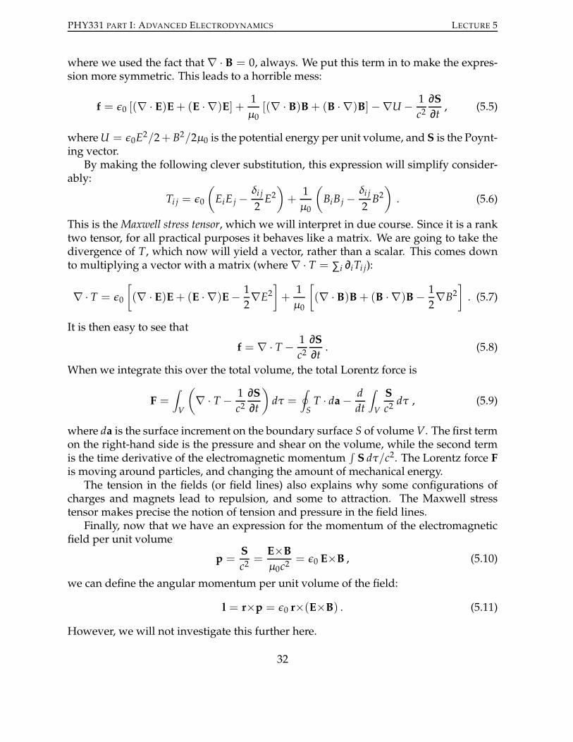
charges and magnets lead to repulsion, and some to attraction. The Maxwell stresstensor makes precise the notion of tension and pressure in the field lines.Finally, now that we have an expression for the momentum of the electromagnetic
field per unit volume
p =S
c2=E×Bµ0c2
= ǫ0 E×B , (5.10)
we can define the angular momentum per unit volume of the field:
l = r×p = ǫ0 r×(E×B) . (5.11)
However, we will not investigate this further here.
32

PHY331 PART I: ADVANCED ELECTRODYNAMICS LECTURE 5
Further reading
– R.H. Good, Classical Electromagnetism, Saunders College Pub. (1999): Sec. 14.2, pp 343-347.
– J.D. Jackson, Classical Electrodynamics, Wiley (1998): Sec. 6.7, pp 258-262.
– R.P. Feynman, Lectures on Physics, volume II, Addison-Wesley (1964): Ch. 27.
– C.A. Brau, Modern Problems in Classical Electrodynamics, Oxford University Press (2004):Sec. 0.6, pp 24-28.
– J. Schwinger, L.L. DeRaad, K.A.Milton, &W. Tsai, Classical Electrodynamics, The AdvancedBook Program, Westview Press (1998): Ch. 3, pp 21-32.
Exercises
1. Write out Maxwell’s stress tensor in matrix form. What does the trace correspondto?
2. Two positive charges move with velocities vA and vB as indicated in the figurebelow. Give a qualitative estimate of the force on charge a and on charge b. Is the
A BvA
vB
Figure 9: Two moving charges.
total momentum conserved in this situation?
3. A photon with energy hω crosses a (ficticious) surface area A in time t. Calculatethe momentum of the photon given that the momentum per unit volume of thefield is given by S/c2.
4. Write the derivation starting with Eq. (5.1) to Eq. (5.5) in index notation.
33

PHY331 PART I: ADVANCED ELECTRODYNAMICS LECTURE 6
6 Multipole expansion and spherical harmonics
Charge and current distributions in a small region of space may be very complicated,and the potentials will generally not be simple. For example, a water molecule is elec-trically neutral as a whole, but one side of the molecule is slightly positive (+q), whilethe other side is slightly negative (−q). If the two charges are separated by a distance d,the potential of each is
Φ+(r) = − q
4πǫ0|r|and Φ−(r) =
q
4πǫ0|r− d|. (6.1)
Using the superposition principle to find the scalar potential of the combined chargesΦ, we find (r≫ d)
Φ(r) = − q|r− d|4πǫ0|r||r− d|
+q|r|
4πǫ0|r||r− d|≃ qd cosθ4πǫ0r2
, (6.2)
where θ measures the angle between d and r. This is the so-called dipole potential. Notethat it is no longer a 1/r potential but falls off faster, with 1/r2. If, for some reasonthe potentials in Eq. (6.1) had different charges q1 and q2 = −q1 − δ, then the scalarpotential would be
Φ(r) = − q14πǫ0|r|
+q1 + δ
4πǫ0|r− d|≃ δ
4πǫ0r+q1d cosθ
4πǫ0r2. (6.3)
Now the scalar potential is a superposition of a monopole and a dipole contribution. Ingeneral, the scalar potential of a charge distribution will have a multipole expansion, andthe same will apply to the vector potential. Let’s look at this in a bit more detail.
6.1 Multipole expansion of a charge density
Suppose that we have a localized (meaning enclosed in a volume V) static charge den-sity ρ(r), which gives rise to a scalar potential
Φ(r) =1
4πǫ0
∫
ρ(r′) dr′
|r− r′| . (6.4)
Far away from the charge density, the potential looks mainly like that of a point charge,but with some higher-order corrections. These corrections are the multipoles, and wecan find them by looking at the Taylor expansion of Eq. (6.4). Let
f (r− r′) =1
|r− r′| =1
√
(x− x′)2 + (y− y′)2 + (z− z′)2. (6.5)
Now we make a Taylor expansion of f (r− r′) around r′ = 0:
f (r− r′) = f (r)−3
∑i=1
r′i∂ f∂ri
∣
∣
∣
∣
r′=0+1
2
3
∑i, j=1
r′ir′j
∂2 f∂ri∂r j
∣
∣
∣
∣
∣
r′=0
+ . . . (6.6)
34

PHY331 PART I: ADVANCED ELECTRODYNAMICS LECTURE 6
dρ
r
r′
r− r′
O
Figure 10: The field at position r far away from a charge distribution ρ(r) can be expressedconveniently in terms of a multipole expansion. O denotes the origin of the coordinate system.
This can be rewritten in compact form as
1
|r− r′| =1
r− r′ · ∇1
r+1
2(r′ · ∇)2
1
r+ . . .
=1
r+3
∑i=1
rir′i
r3+1
2
3
∑i, j=1
ri(3r′ir′j − r′
2δi j)r j
r5+ . . . (6.7)
where r =√
r21 + r22 + r23 = |r| is the magnitude of the vector with components ri. Aftersubstituting this into the generic form of the scalar potential in Eq. (6.4), we find
Φ(r) =1
4πǫ0
∫
ρ(r′) dr′
r+1
4πǫ0
3
∑i=1
∫
r′irir3
ρ(r′) dr′
+1
8πǫ0
3
∑i, j=1
∫ 3r′ir′j − r′
2δi j
r5rir jρ(r′) dr′ + . . . (6.8)
=1
4πǫ0
[
Q
r+3
∑i=1
Qirir3
+1
2
3
∑i, j=1
riQi jr j
r5+ . . .
]
. (6.9)
The multipole moments of the charge distribution are the total charge Q, the dipole mo-ment Qi, the quadrupolemoment Qi j, etc. They are defined as follows:
Q =∫
ρ(r′) dr′ (6.10)
Qi =∫
r′i ρ(r′) dr′ (6.11)
Qi j =∫
(3r′ir′j − r′
2δi j)ρ(r′) dr′ (6.12)
... (6.13)
35

PHY331 PART I: ADVANCED ELECTRODYNAMICS LECTURE 6
The quadrupole moment has nine components, but it is easy to see that Qi j = Q ji, and
3
∑i=1
Qii =3
∑i=1
∫
(3riri − r2)ρ(r) dr =∫
[(
33
∑i=1
riri
)
− 3r2]
ρ(r) dr = 0 . (6.14)
The quadrupole moment is therefore characterised by five independent variables.
6.2 Spherical harmonics and Legendre polynomials
It is clear from the previous section that we can continue the multipole expansion tooctupoles and higher, but it is also pretty obvious that the polynomials in the definitionsof Qi jk... get quite unwieldy very quickly. Luckily, there is a more systematic approachbased on spherical harmonics. These are functions of the spherical coordinates θ andφ ofa vector r, and the function f can then be written as
1
|r− r′| =∞
∑l=0
+l
∑m=−l
r′ l
rl+1
√
4π
2l + 1Ylm(θ,φ)
√
4π
2l + 1Y∗lm(θ′,φ′) (6.15)
with
Ylm(θ,φ) =
√
2l + 1
4π
(l +m)!
(l −m)!
eimφ
sinmθ
[
d
d cosθ
]l−m (cos2θ − 1)l2ll!
. (6.16)
This is still rather complicated, but the advantage is that this is valid for all l. Note alsothat the spherical harmonics are complex, but Eq. (6.15) is still real due to the sum overm. You should think of the Ylm as basis functions that can be used to write arbitraryfunctions (of θ and φ) as a series, just like any polynomial can be written as a series
∑n anxn, or a periodic function as a Fourier series. Like any proper set of basis functions,the Ylm obey an orthogonality relation:
∫
dΩ Y∗lm(θ,φ)Yl′m′(θ,φ) ≡∫ π
0sinθ dθ
∫ 2π
0dφ Y∗lm(θ,φ)Yl′m′(θ,φ) = δll′δmm′ , (6.17)
where we introduced the integration over the sold angle dΩ.We can now define the Legendre polynomials as
Pl(w) =
[
d
dw
]l (w2 − 1)l2l l!
, (6.18)
with normalisation Pl(1) = 1. In the spherical harmonics, we have set w = cosθ. TheLegendre polynomials also obey an orthogonality relation
∫ 1
−1dw Pl(w)Pl′(w) =
2
2l + 1δll′ . (6.19)
36
PHY331 PART I: ADVANCED ELECTRODYNAMICS LECTURE 6
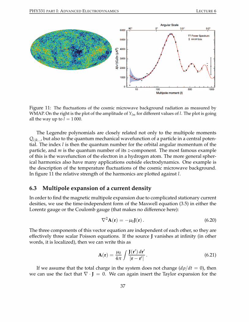
Figure 11: The fluctuations of the cosmic microwave background radiation as measured byWMAP. On the right is the plot of the amplitude of Ylm for different values of l. The plot is goingall the way up to l = 1 000.
The Legendre polynomials are closely related not only to the multipole momentsQi jk..., but also to the quantummechanical wavefunction of a particle in a central poten-tial. The index l is then the quantum number for the orbital angular momentum of theparticle, and m is the quantum number of its z-component. The most famous exampleof this is the wavefunction of the electron in a hydrogen atom. The more general spher-ical harmonics also have many applications outside electrodynamics. One example isthe description of the temperature fluctuations of the cosmic microwave background.In figure 11 the relative strength of the harmonics are plotted against l.
6.3 Multipole expansion of a current density
In order to find the magnetic multipole expansion due to complicated stationary currentdesities, we use the time-independent form of the Maxwell equation (3.5) in either theLorentz gauge or the Coulomb gauge (that makes no difference here):
∇2A(r) = −µ0J(r) . (6.20)
The three components of this vector equation are independent of each other, so they areeffectively three scalar Poisson equations. If the source J vanishes at infinity (in otherwords, it is localized), then we can write this as
A(r) =µ0
4π
∫
J(r′) dr′
|r− r′| . (6.21)
If we assume that the total charge in the system does not change (dρ/dt = 0), thenwe can use the fact that ∇ · J = 0. We can again insert the Taylor expansion for the
37

PHY331 PART I: ADVANCED ELECTRODYNAMICS LECTURE 6
function 1/|r− r′| given by Eq. (6.6), which leads to
Ai(r) =µ0
4π
[
1
r
∫
Ji(r′) dr′ +
1
r3
3
∑j=1
∫
r jr′j Ji(r
′) dr′ +O(r−5)
]
. (6.22)
The first term in square brackets is the magnetic monopole term, which we expect tovanish for magnetostatics, and the second term is the magnetic dipole moment.To show that the magnetic monopole contribution vanishes for all J(r), note that
∫
Ji(r′) dr′ =
3
∑j=1
∫
J j(r′)
∂r′i∂r′jdr′. (6.23)
Integration by parts of the right-hand side of this expression gives
∫
Ji(r′) dr′ =
3
∑j=1
∫
J j(r′)r′i d
2r′k 6= j
∣
∣
∣
∣
r′j=∞
r′j=−∞
−3
∑j=1
∫
r′i∂J j(r′)
∂r′jdr′ . (6.24)
The first term of the right-hand side is zero because the current density at infinity is zero:we consider a localized current density. The differential in the second term (together withthe sum) is ∇ · J, which, we already determined, is zero.The magnetic dipole moment is therefore the lowest order term in Eq. (6.22). Let’s
separate it into the symmetric and anti-symmetric parts:
r′j Ji =1
2
(
r′j Ji + r′i J j
)
+1
2
(
r′j Ji − r′i J j)
. (6.25)
The integral over the symmetric part is zero. You can see this by integration by parts:
3
∑j=1
r j
∫
(
r′j Ji + r′i J j
)
dr′ =3
∑j,k=1
r j
∫
(
r′j∂r′i∂r′kJk + r
′i
∂r′j∂r′kJ j
)
dr′
=3
∑j,k=1
r j
[
∫
r′jr′i Jkd
2rl 6=k
∣
∣
∣
∣
r′k=∞
r′k=−∞
−∫
r′i∂J j(r′)
∂r′jdr′]
= 0 . (6.26)
In the first line we again used the Kronecker delta representation ∂ri/∂r j = δi j, and inthe second line we used the same tricks to show that the monopole moment is zero.The lowest order moment of the vector potential is therefore
Ai(r) =µ0
8πr3
3
∑j=1
∫
r j
(
r′j Ji(r′)− r′i J j(r′)
)
dr′ . (6.27)
It is very tempting to write the antisymmetric part r′j Ji − r′i J j as a cross product. Thisleads to the definition of the magnetic dipole moment of the current distribution
m =1
2
∫
r×J(r) dr . (6.28)
38

PHY331 PART I: ADVANCED ELECTRODYNAMICS LECTURE 6
However, we can’t just plug the expression for m in Eq. (6.28) into Eq. (6.27), becausethe components do not match up: The cross product (r j Ji − ri J j) in Eq. (6.27) makes useof component i, which according to the equation should contribute to Ai. This is notpossible unless another cross product is involved. If we call 12
∫
(r j Ji − ri J j)dr′ = mkwith k 6= i, j, then we have the equation
Ai(r) =µ0
4πr3
3
∑j=1( 6=i)
∑k 6= j,ir jmk . (6.29)
You see that the Ai component depends on terms r j and mk, with neither j nor k equalto i. This is crying out for another cross product, and it will involvem and r. So let’s seeif we can massagem×r such that we obtain Eq. (6.27):
(m×r)i =3
∑j=1
1
2
∫
(
r jr′j Ji − r jr′i J j
)
dr′ . (6.30)
The integrand involves the antisymmetric part of r′j Ji. However, since we have justproved that the integration over the symmetric part is zero, we can add this to theintegrand without affecting the integral. But adding the symmetric and anti-symmetricpart of r′j Ji is just r
′j Ji, and the cross product becomes
(m×r)i =3
∑j=1
1
2
∫
r jr′j Ji(r
′) dr′ . (6.31)
This leads immediately to the vector potential of a magnetic dipole:
A(r) =µ0
4π
m×rr3. (6.32)
Further reading
– R.H. Good, Classical Electromagnetism, Saunders College Pub. (1999): Ch. 7, pp 164-182.
– J.D. Jackson, Classical Electrodynamics, Wiley (1998): Sec 4.1 & 5.6, pp 145-150, 184-188.
– B.I. Bleaney & B. Bleaney, Electricity and magnetism, Vol. 1, Oxford University Press (1976):Sec. 1.4, 2.3 & 4.2, pp 11-14, 38-43, 101-107.
– J.R. Reitz, F.J. Milford, & R.W. Christy, Foundations of Electromagnetic Theory, fourth edition,Addison-Wesley (1993): Sec. 2.9, pp 46-48.
– J. Schwinger, L.L. DeRaad, K.A.Milton, &W. Tsai, Classical Electrodynamics, The AdvancedBook Program, Westview Press (1998): Ch. 22, pp 257-264.
39

PHY331 PART I: ADVANCED ELECTRODYNAMICS LECTURE 6
Exercises
1. Let the charge distribution ρ(r, t) consist of two static charges ρ(r, t) = qδ(r) −qδ(r−d). Calculate the total charge Q, the dipole moment Qi, and the quadrupolemoment Qi j by evaluating Eqs. (6.10), (6.11), and (6.12). How does the position ofthe origin affect the outcome?
2. A sphere of radius R rotates with angular velocity ω around a symmetry axis,and carries a uniformly distributed surface charge Q. Give the charge and currentdensities ρ and J, and verify that ∇ · J = 0.
3. The magnetic moment of an electron is one Bohr magneton, µB = eh/2m. Supposewe model this as a small ring current of radius r, which can be considered the sizeof the electron. What is the smallest possible size of the electron according to thismodel? Experimentally, the electron behaves as if it is a point particle. Is this aproblem for this model?
4. Verify Eqs. (6.7) and (6.8).
40
PHY331 PART I: ADVANCED ELECTRODYNAMICS LECTURE 7
7 Dipole fields and radiation
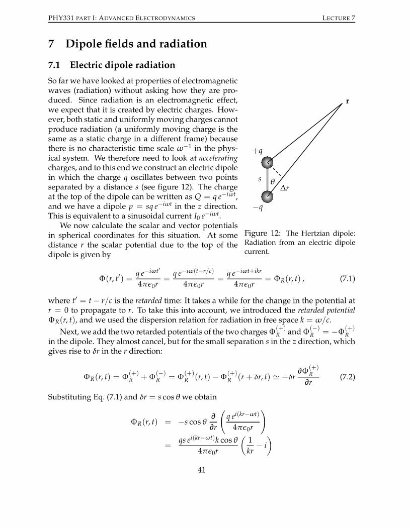
7.1 Electric dipole radiation
s θ
+q
−q
∆r
r
Figure 12: The Hertzian dipole:Radiation from an electric dipolecurrent.
So far we have looked at properties of electromagneticwaves (radiation) without asking how they are pro-duced. Since radiation is an electromagnetic effect,we expect that it is created by electric charges. How-ever, both static and uniformlymoving charges cannotproduce radiation (a uniformly moving charge is thesame as a static charge in a different frame) becausethere is no characteristic time scale ω−1 in the phys-ical system. We therefore need to look at acceleratingcharges, and to this endwe construct an electric dipolein which the charge q oscillates between two pointsseparated by a distance s (see figure 12). The chargeat the top of the dipole can be written as Q = q e−iωt,and we have a dipole p = sq e−iωt in the z direction.This is equivalent to a sinusoidal current I0 e
−iωt.We now calculate the scalar and vector potentials
in spherical coordinates for this situation. At somedistance r the scalar potential due to the top of thedipole is given by
Φ(r, t′) =q e−iωt
′
4πǫ0r=q e−iω(t−r/c)
4πǫ0r=q e−iωt+ikr
4πǫ0r= ΦR(r, t) , (7.1)
where t′ = t− r/c is the retarded time: It takes a while for the change in the potential atr = 0 to propagate to r. To take this into account, we introduced the retarded potentialΦR(r, t), and we used the dispersion relation for radiation in free space k = ω/c.
Next, we add the two retarded potentials of the two chargesΦ(+)R andΦ
(−)R = −Φ
(+)R
in the dipole. They almost cancel, but for the small separation s in the z direction, whichgives rise to δr in the r direction:
ΦR(r, t) = Φ(+)R + Φ
(−)R = Φ
(+)R (r, t) −Φ
(+)R (r+ δr, t) ≃ −δr
∂Φ(+)R
∂r(7.2)
Substituting Eq. (7.1) and δr = s cosθ we obtain
ΦR(r, t) = −s cosθ ∂∂r
(
q ei(kr−ωt)
4πǫ0r
)
=qs ei(kr−ωt)k cosθ
4πǫ0r
(
1
kr− i)
41

PHY331 PART I: ADVANCED ELECTRODYNAMICS LECTURE 7
=pRk cosθ
4πǫ0r
(
1
kr− i)
, (7.3)
where pR is the retarded dipole moment.The vector potential of this oscillating dipole in spherical coordinates is
AR(r, t) =µ0
4π
∫
JR(r, t)
rdV =
1
4πǫ0c2rI0 ei(kr−ωt) s =
1
4πǫ0c2rIR s , (7.4)
where s is the dipole vector s(cosθ r − sinθ θ), parallel to the z axis, and IR is the re-tarded current in the dipole. Using the relations Q = q e−iωt and I = dQ/dt, we canwrite the dipole moment pR in the scalar potential in terms of IR:
pR =is
ωIR . (7.5)
We therefore have
ΦR(r, t) =IRs cosθ
4πǫ0cr
(
1+i
kr
)
and AR(r, t) =IRs(cosθ r− sinθ θ)
4πǫ0c2r. (7.6)
The electric field E is given by E = −∇ΦR − AR. Using the derivatives in sphericalcoordinates we find
Er(r, t) = −∂ΦR
∂r− (AR)r =
kIRs cosθ
4πǫ0cr
(
2
kr+2i
(kr)2
)
,
Eθ(r, t) = −1r
∂ΦR
∂θ− (AR)θ =
kIRs sinθ
4πǫ0cr
(
1
kr+
i
(kr)2− i)
. (7.7)
We already know that radiation carries energy, so the total energy flux through a closedsurface around the source is constant. If we take the surface to be that of a spherewith radius r, the energy flux 4πr2(ǫ|E|2/2+ |B|2/2µ0) must be constant for all r. Theradiating part of the E and B fields are therefore proporional to 1/r. Looking at Eq. (7.7),we see that the only contribution to the radiation is due to the i term in Eθ. Similarly,the only contributing term of the B field is (see exercise)
Bφ(r, t) = −i kIRs sinθ
4πǫ0c2r=Eθ(r, t)
c, (7.8)
where Eθ(r, t) now denotes the radiating part of the E field. Poynting’s vector is givenby
Se =ReEθ×ReBφ
µ0= Re
E×B∗µ0
=1
16π2ǫ0c
(
ksI sinθ
r
)2
r . (7.9)
Note that we can calculate the Poynting vector by taking the complex conjugate of the Bfield and take the real part of S afterards. Again, it is often much easier to calculate withcomplex phase factors of the form eiϕ than with the trigonometric counterparts sinϕ,cosϕ and tanϕ.
42

PHY331 PART I: ADVANCED ELECTRODYNAMICS LECTURE 7
E
B
Figure 13: The directions of the E and B fields of a spherical wave radiated by a dipole in thecentre. After half the oscillation period the fields point in the opposite direction.
7.2 Magnetic dipole radiation
s
s
θ
I
r
Figure 14: Radiation from a mag-netic dipole current.
Now suppose we have a small current going in asquare loop of area s2, leading to a magnetic dipolemoment m = s2 I0 e
−iωt. The current is changing intime in a periodic way. Again, we can define the re-tarded magnetic dipole by substituting t → t− r/c. Ifthe current has a low impedance the scalar potential iszero, while the vector potential is
AR(r, t) =µ0mRk sinθ
4πr
(
− 1kr
+ i
)
φ . (7.10)
We can again field the radiating parts of the E and Bfields via E = −A and B = ∇×A:
Eφ =µ0mRk
2c sinθ
4πr= −cBθ , (7.11)
and the Poynting vector is
Sm = ReE×B∗2µ0
=1
16π2ǫ0c
[
(ks)2 I sinθ
r
]2
r . (7.12)
The difference between Se and Sm is a factor (ks)2 .
7.3 Larmor’s formula
Clearly, radiation is generated by accelerated charges and changing currents. In theprevious sections we have looked at periodically changing charges and currents, but
43

PHY331 PART I: ADVANCED ELECTRODYNAMICS LECTURE 7
in many situations the charges and currents change in an aperiodic way. For example,when a charge is kicked, it will emit a burst of radiation. We will now consider thequestion of how much power P is radiated when a charge is accelerated by an amounta. This will lead to Larmor’s formula.
Joseph Larmor(1857-1942)
Suppose a particle with charge q follows a trajectoryrq(t). We can formally associate a dipole moment p to thisparticle:
p(t) = q rq(t) . (7.13)
The current due to the motion of the charge is clearly re-lated to the velocity vq, so we can write
I =dp
dt= qdrq
dt= q vq(t) . (7.14)
The acceleration aq of the particle is proportional to thesecond derivative of the dipole moment:
d2p
dt2= q aq(t) . (7.15)
Next, we calculate the vector potential and the magnetic field B of the moving charge.First, we note that the current I is the spatial integration over the current density, so
we have
A(r, t) =µ0
4πr
∫
J(r′, t− r/c) dr′ =µ0
4πrIR =
µ0
4πr
dp
dt(t− r/c) , (7.16)
evaluated at the retarded time, because the field needs time to propagate from the chargeto the point where the vector potential is calculated.The magnetic field is found using B = ∇×A. We need to keep in mind two things:
(1) We can ignore all the contributions that do not scale like 1/r, because they do notpropagate. (2) We must remember that the time variable depends on r because weconsider the retarded time. The magnetic field is then
B(r, t) = ∇×A(r, t) =µ0
4π
[
∇×(
1
r
)
dp
dt+1
r∇×dpdt
]
=µ0
4πr∇×dpdt, (7.17)
where the last equality holds because∇×(1/r) leads to a non-propagating contributionto the field. The calculation of the curl of dp/dt is a bit tricky, so we’ll do it here in somedetail. In particular, it is convenient to use index notation:
(
∇×dpdt
)
i
= ǫi jk∂ j(
dp
dt
)
k
. (7.18)
Using the chain rule, we can write (t = tq − r/c with )
∂ j =∂t
∂x jd
dt= −1
c
x j
r
d
dt, (7.19)
44

PHY331 PART I: ADVANCED ELECTRODYNAMICS LECTURE 7
which allows us to rewrite the cross product:
(
∇×dpdt
)
i
= −1cǫi jkx j
r
(
d2p
dt2
)
k
. (7.20)
In vector notation, this becomes
∇×dpdt
= − 1crr×d
2p
dt2= −1
cr×d
2p
dt2= −q
cr×aq , (7.21)
and therefore the B field can be written as
B(r, t) =µ0
4πr∇×dpdt
= − µ0
4πcrr×d
2p
dt2= − qµ0
4πcrr×aq , (7.22)
evaluated at time t, and due to an accelerated charge at the retarded time t− r/c.The radiating part of the electric field E must be perpendicular to the radiating part
of the magnetic field that we just calculated, and they differ by a factor c. Keeping thecorrect handedness, the radiating E field can be written as a cross product between Band r:
E(r, t) = cB×r = − qµ04πr
(
r×aq)
×r . (7.23)
Now that we know the E and B fields, we can calculate the Poynting vector S, whichgives the energy flux through a surface. If we take the surface to be a sphere with radiusR surrounding the accelerating charge, we can calculate the total radiated power
P =∮
SS · R R2 dΩ , (7.24)
where dΩ is a solid angle.The Poynting vector is straightforward to calculate:
S =E×Bµ0
=µ0q
2
16π2cr2[(
r×aq)
×r]
×(
r×aq)
. (7.25)
Using the vector identity A×(B×C) = B(A ·C)− C(A · B) we rewrite this as
S =q2
16π2ǫ0c3r2[
aq − r(aq · r)]
×(
r×aq)
=q2
16π2ǫ0c3r2
r[
|aq|2 − (aq · r)2]
− aq(
aq · r− aq · r)
=q2
16π2ǫ0c3r2
[
a2q − (aq · r)2]
r
=q2 a2q sin
2θ
16π2ǫ0c3r2r , (7.26)
45
PHY331 PART I: ADVANCED ELECTRODYNAMICS LECTURE 7
where we defined aq = |aq| and we oriented our coordinate system such that the accel-eration is along the z direction. The inner product aq · r is therefore equal to aq cosθ.The radiated power through a sphere surrounding the accelerating charge is now
straightforward to calculate:
P =∮
SS · R R2 dΩ =
∮
S
q2 a2q sin2θ
16π2ǫ0c3R2R2 dΩ =
q2 a2q
16π2ǫ0c3
∫ π
0
∫ 2π
0sin2θ dθ dφ . (7.27)
The integral over sin2θ is equal to 8π/3, so we arrive at
P =1
4πǫ0
2q2 a2q
3c3. (7.28)
This is the celebrated Larmor formula, derived by Joseph Larmor in 1897.
Further reading
– R.H. Good, Classical Electromagnetism, Saunders College Publishing (1999): Sec. 15.1 &15.2, pp 371-379.
– J.D. Jackson, Classical Electrodynamics, Wiley (1998): Sec. 9.1-9.3 pp 407-416.
– R.P. Feynman, Lectures on Physics, volume II, Addison-Wesley (1964): Ch. 21.
– J.R. Reitz, F.J. Milford, & R.W. Christy, Foundations of Electromagnetic Theory, fourth edition,Addison-Wesley (1993): Ch. 20, pp 525-544.
– J. Schwinger, L.L. DeRaad, K.A.Milton, &W. Tsai, Classical Electrodynamics, The AdvancedBook Program, Westview Press (1998): Ch. 32-33, pp 351-366.
Exercises
1. Atoms can have both an electric and a magnetic dipole that produces radiation.Which of these typically two produces stronger radiation?
2. Consider again the Bohr model, in which an electron orbits a proton. The size ofthe orbit is given by the Bohr radius (5.29 · 10−11 m), and the angular momentumof the ground state is h = 1.05 · 10−34 Js. According to classical electrodynamics,how strong is the radiated power? Give an order-of-magnitude estimate of thelifetime of the atom.
46

PHY331 PART I: ADVANCED ELECTRODYNAMICS LECTURE 8
8 Electrodynamics in macroscopic media
8.1 Macroscopic Maxwell equations
So far, we have considered the fields of (moving) charges and the interactions betweenthe charges. In principle, this covers all classical electromagnetic phenomena, since allmatter is made up of charged particles that interact with each other. However, if weare dealing with 1023 atoms we don’t want to solve the Maxwell equations for everyindividual atom. Especially when the time and length scales relevant to our problemare large compared to that of the atoms, we much rather average over the atomic fieldsand have effective fields in the media.The electric and magnetic fields in Maxwell’s equations are now average fields 〈E〉
and 〈B〉, and the charge and current densities 〈ρ〉 and 〈J〉 now consist of free chargesand currents as well as bound charges and currents. Maxwell’s equations in macroscopicmedia then become
∇ · 〈B〉 = 0 and ∇×〈E〉+∂〈B〉
∂t= 0 (8.1)
∇ · 〈E〉 =〈ρ〉ǫ0
and ∇×〈B〉 −µ0ǫ0∂〈E〉
∂t= µ0〈J〉 . (8.2)
The charge and current densities are
〈ρ〉 = ρ f + ρb and 〈J〉 = J f + Jb (8.3)
where the subscripts f and b denote “free” and “bound”, respectively.The fields in the materials are no longer the bare E and B fields due to freely moving
charges and currents (as was the case for the microscopic Maxwell equations), but theyare modified by the presence of the bound charges and currents. We want to relatethe modified fields to material properties (the bound charges and currents) and modifyMaxwell’s equations such that they involve the macroscopic fields and the free chargesand currents.
8.2 Polarization and Displacement fields
First, we consider a material that has bound charges. These are, for example, electronsthat cannot move freely through the material, but that are bound to the parent molecule.When an external electric field is applied, the negative electrons move with respect tothe positive nuclei, creating a small dipole moment. This dipole moment is alignedagainst the external field, because the external field pulls the charges such that the localfield becomes smaller. All these little dipole moments create a macroscopic field P,which is related to the bound charge density via
ρb = −∇ · P . (8.4)
47

PHY331 PART I: ADVANCED ELECTRODYNAMICS LECTURE 8
+
+
+
+
+
+++
+++
+
+++
++
++ +
+
+
+
+++
++
+
+++
++
++
Uniform polarization Nonuniform polarization
Figure 15: Polarization in a medium
This is in some sense the definition of P. Wemust now relate the P to the dipole momentsof the molecules.Let V be the volume of the medium, and the dipole density in the i direction is ρbri.
Then∫
Vriρb dr = −
3
∑j=1
∫
Vri
∂Pj∂r jdr = −
3
∑j=1
∫
SriPj d
2rk 6= j
∣
∣
∣
∣
r jonS
r jonS
+∫
VPi dr , (8.5)
where the first equality comes from Eq. (8.4), and the second comes from partial inter-gration. The surface term is zero when we take the surface just outside the medium. Invector notation, we therefore have
∫
Vrρb dr =
∫
VP dr = ∑
V
pn , (8.6)
where the last term is the sum of all microscopic dipole moments in the volume V.Outside V we have P = 0.Now that we know what P means, we can rewrite the Maxwell equation ∇ · 〈E〉 =
〈ρ〉/ǫ0 using Eqs. (8.3) and (8.4)as
∇ · 〈E〉 =ρ f + ρb
ǫ0=
ρ f
ǫ0− 1
ǫ0∇ · P . (8.7)
Considering we want the macroscopic field in terms of the free charges, we can definethe macroscopic field as the displacement field D:
D = ǫ0〈E〉+ P (8.8)
All the material properties are determined by P. The correspondingmacroscopic Maxwellequation is then
∇ ·D = ρ f (8.9)
Often the polarization field is directly proportional to E, and we write P = χǫ0E,where χ is the susceptibility of the medium. The displacement field then becomes
D = ǫ0(1+ χ)E ≡ ǫ0ǫrE ≡ ǫE . (8.10)
48

PHY331 PART I: ADVANCED ELECTRODYNAMICS LECTURE 8
Assuming for the moment that the permeability µ0 does not change, one can see imme-diately that the wave equation yields a propagation velocity c2/ǫr. In ordinary materi-als, we therefore have ǫr ≥ 1. As we will see in the next lecture, this is directly relatedto the index of refraction.Some materials have a non-isotropic response to the electric field, for example
Pi = ǫ0
3
∑j=1
χi jE j , (8.11)
where the polarization in the i direction depends in some way on the E field in the x,y, and z direction, while the polarization in the k 6= i direction depends on the sameexternal E field in a different way. The susceptibility is therefore in general a tensor.Clearly, such a medium has an intrinsic orientation. When the medium is transparent, amedium like this gives rise to birefringence, where light with different polarizations (notto be confused with P) is bent differently when it enters the medium.Other materials have a polarization field P that depends on the external field E in a
nonlinear way:
Pi = ǫ0
(
χ(0)i +
3
∑j=1
χ(1)i j E j +
3
∑j,k=1
χ(2)i jk E jEk +
3
∑j,k,l=1
χ(3)i jklE jEkEl + . . .
)
. (8.12)
The susceptibility has different orders χ(n)i...l corresponding to the n
th power in the exter-nal field. In practice, we consider only the effects up to third order, since higher order
effects tend to be extremely weak. The χ(2) term is responsible for frequency doubling
materials, among other things, and the χ(3) term can be used to induce optical phaseshifts that are proportional to the intensity of a second field. It is also called the Kerrnonlinearity.
8.3 Magnetization and Magnetic induction
Now we will construct the macroscopic magnetic field using the free and bound cur-rents. Apart from the free currents in the material, there may be bound currents thatare confined to the molecules. In quantum mechanics these bound currents can be thespins of the electrons and nuclei, but let’s keep things classical for now.The bound currents may be due to a change of bound charges, which can be written
as ∂P/∂t. Alternatively, they may correspond to little current loops, which give rise to amicroscopic magnetic dipole moment. Under the influence of an external field B, theselittle magnets can line up to form a macroscopic field that we shall denote by∇×M. Wethen have the following expression for the bound current:
Jb =∂P∂t
+∇×M (8.13)
49

PHY331 PART I: ADVANCED ELECTRODYNAMICS LECTURE 8
Uniform magnetization Nonuniform magnetization
Figure 16: Magnetization in a medium
The divergence of the bound charge is
∇ · Jb =∂∇ · P
∂t+∇ · (∇×M) = −∂ρb
∂t= 0 , (8.14)
since the bound charge is conserved.Now let’s consider the second inhomogeneous Maxwell equation
∇×〈B〉 −µ0ǫ0∂〈E〉
∂t= ∇×〈B〉 −µ0ǫ0
∂∂t
(
D
ǫ0− P
ǫ0
)
= µ0〈J〉 = µ0
(
Jb + J f
)
. (8.15)
This leads to
∇×〈B〉 −µ0∂D∂t
+ µ0∂P∂t
= µ0∂P∂t
+ µ0∇×M+ µ0J f . (8.16)
We can now define the magnetic field H in terms of the magnetic induction B and themacroscopic magnetizationM as
H =1
µ0〈B〉 −M , (8.17)
yielding the Maxwell equation
∇×H− ∂D∂t
= J f (8.18)
The homogeneous Maxwell equations remain unchanged, since here E and B arefundamental (that is, nomaterial properties are present in these equations). Also, for themacroscopic case it is understood that all fields are averages, and we drop the brackets〈.〉. The macroscopic Maxwell equations then become
∇ · B = 0 and ∇×E+∂B∂t
= 0 (8.19)
∇ ·D = ρ f and ∇×H− ∂D∂t
= J f . (8.20)
50

PHY331 PART I: ADVANCED ELECTRODYNAMICS LECTURE 8
Further reading
– R.H. Good, Classical Electromagnetism, Saunders College Publishing (1999): Ch. 9 & 10, pp204-277.
– J.D. Jackson, Classical Electrodynamics, Wiley (1998): Sec. 4.3-4.6 & 5.8, pp 151-165, 191-194.
– R.P. Feynman, Lectures on Physics, volume II, Addison-Wesley (1964): Ch. 11 & 36.
– W.J. Duffin, Electricity and Magnetism, McGraw-Hill (1990): Ch. 11, 12, pp 282-335.
– J.R. Reitz, F.J. Milford, & R.W. Christy, Foundations of Electromagnetic Theory, fourth edition,Addison-Wesley (1993): Ch. 4 & 9, pp 97-126, 218-255.
– C.A. Brau, Modern Problems in Classical Electrodynamics, Oxford University Press (2004):Sec. 6.1, pp 282-293.
– J. Schwinger, L.L. DeRaad, K.A.Milton, &W. Tsai, Classical Electrodynamics, The AdvancedBook Program, Westview Press (1998): Ch. 4, pp 33-44.
Exercises
1. A slab of linear dielectric material is placed inside a capacitor. The dielectric doesnot fill the space inside the capacitor completely. Determine the field lines of E, P,and D between the capacitor plates.
2. A slab of linear dielectric material is placed inside a capacitor. The dielectric slaband the plates of the capacitor are square with side w, and the thickness of the slabis s. The plates are held at constant potential V.
w
x
s F
V
(a) Write down the energy in a capacitor.
(b) How does the charge on the plates change? Does this change the energy ofthe capacitor?
(c) Calculate the force on the dielectric slab.
3. A one-dimensional dielectric has a nonlinear polarization field given by
P(t) = χ(1)E(t) + χ(2)E(t)2 .
If the incoming wave is described by E(t) = E0 cosωt show that the dielectricgives rise to a wave with double the frequency. What happens when the incomingwave is a superposition of two frequenciesω1 andω2? (Hint: write the waves inexponential notation.)
51

PHY331 PART I: ADVANCED ELECTRODYNAMICS LECTURE 9
9 Waves in dielectric and conducting media
From our everyday experience it is clear that electromagnetic radiation (in particularlight) is able to propagate through some media, but not through others. Light has noproblem travelling through air and glass, but when it hits a conductor, most of it willbe reflected. In this lecture we investigate why this is, and what are the characteristicfeatures of different media.
Georg Ohm (1789-1854)
When waves penetrate a medium, the molecules in themedium respond to the electric field and the magneticinduction to form polarization and magnetization fields.Let’s assume that the medium is electrically neutral, sothat there are no free charges (ρ = 0), but there may beelectrons in a conduction band that can produce free cur-rents J. These electrons presumably respond directly tothe electric field, such that the free current is propotionalto E:
J = σE (Ohm’s law). (9.1)
This is Ohm’s law, and the constant of proportionality σ isthe conductance. This law has a wide range of applicability,but you should be aware that there are many interestingsituations where Ohm’s law does not hold.There are essentially three regimes of interest for σ : (1)
σ is small, and the medium is a dielectric; (2)σ is large, and the medium is a conductor;or (3)σ is imaginary, and the medium is a plasma. Wewill derive the index of refractionfor dielectrics, the skin depth for conductors, and the plasma frequency for plasmas. Wewill also derive the reflectivity of these three types of materials.
9.1 Waves in dielectric media
First, we rederive the wave equations from the Maxwell equations, but this time wekeep the J term. We find the following differential equations for E and B:
∇2E−µǫ∂2E∂t2
= µ∂J∂t, (9.2)
∇2B− µǫ∂2B∂t2
= −µ∇×J , (9.3)
where ǫ = ǫrǫ0 and µ = µrµ0. Using Ohm’s law, this leads to
∇2E−µǫ∂2E∂t2
− µσ∂E∂t
= 0 , (9.4)
∇2B− µǫ∂2B∂t2
−µσ∂B∂t
= 0 . (9.5)
52

PHY331 PART I: ADVANCED ELECTRODYNAMICS LECTURE 9
Air Dielectric Air Dielectric(a) (b)
E fields B fields
Figure 17: Waves incident on a dielectric. The waves propagate in the dielectric. (a) The electricfield is mostly transmitted, and the reflected wave experiences a phase shift. (b) The magneticfield is mostly transmitted, and the reflected wave does not experience a phase shift.
We substitute again the plane wave solutions for waves in the positive z direction E =
E0ei(kz−ωt) and B = B0e
i(kz−ωt), and we immediately find that
k =√
ǫµω2 + iωµσ = k0√
µrǫr
√
1+iσ
ωǫ, (9.6)
where k0 = ω/c. You can see that the wave vector k is complex!Now we can look at the three different regimes for σ . If the conductance is small
(σ/ωǫ ≪ 1), the medium is a dielectric and the imaginary root is approximately equalto 1. The wave vector is real, so the waves propagate freely. However, the value of thewave vector is modified by the factor
√ǫrµr. It turns out that this is indeed the index of
refraction, at least for apolar materials4.The reflectivity of a dielectric can be calculated as well. For ordinary dielectrics
where D = ǫE and B = µH, the ratio between the electric field and the magneticinduction is given by the velocity of the wave in the medium:
E
B=
c√ǫrµr
. (9.7)
In air, this leads to approximately E = cB, and the (average) Poynting vector in amedium is then
Sav = nǫ0cE2rms , (9.8)
where n is the index of refraction, and E2rms is the average strength to the electric fieldsquared.
4In apolar media the distribution of the electrons in the molecules is fast enough to follow the oscillat-ing fields. In polar materials, however, the response of the medium is slow since the polar molecules haveto re-orient themselves. This is the principle behind the microwave: The water molecules try to realignthemselves with an oscillating microwave field, and as a consequence the water gets heated.
53

PHY331 PART I: ADVANCED ELECTRODYNAMICS LECTURE 9
In order to calculate the reflectivity, we need to figure out what the boundary con-ditions are for the different fields at the separation of the medium and the air. We willconsider the difference between the fields just outside the medium and the field justinside the medium. From ∇ ·D = ρ we find that
∆Dn = D1,n −D2,n = σf , (9.9)
where the subscript n denotes the normal component with respect to the surface, andthe 1 and 2 denote the field outside and inside themedium, respectively. σf is the surfacecharge. From ∇ · B = 0 we find that
∆Bn = B1,n − B2,n = 0 . (9.10)
Air Medium
l l
∆z
Figure 18: Boundary condi-tions on a dielectric surface.
The boundary condition for ∆Et is more complicated.From ∇×E = −B we have (see Fig. 18)
∮
E · dl = −∫ ∂B
∂t· da , (9.11)
where the contour is taken as a rectangle perpendicularto the surface and sticking half-way into the surface. Theparallel sides of the loop have length l, and the sides per-pendicular to the surface have length ∆z. We thereforehave
l(E1,t − E2,t) = −l∆z∂B∂t
= 0 , (9.12)
where the last equality follows from taking the limit ∆z→0. We therefore have the third boundary condition
∆Et = E1,t − E2,t = 0 . (9.13)
Finally, we establish the boundary condition for the transverse magnetic field ∆Ht.There may be infinite bound surface current densities Jb, so we use ∇×H = J + D,which ignores Jb. The free surface current will be denoted by Kf, and the last boundarycondition reads
∆Ht = H1,t −H2,t = Kf . (9.14)
Now we can state the relations between the incident (I), reflected (R), and transmittedfields (T):
EI − ER = ET and BI + BR =BTµr. (9.15)
Note that the reflected B field picks up a relative minus sign. This is because the Poynt-ing vector must point in the opposite way to the incident wave, and from Eq. (9.7) weknow that the magnetic induction must gain in relative strength in the medium.
54

PHY331 PART I: ADVANCED ELECTRODYNAMICS LECTURE 9
Now assume that the medium is such that µr = 1. We then have
B =nk
ωE , (9.16)
which leads toEI + ER = nET . (9.17)
Together with ET = EI − ER, this yields the ratio
EREI
=n− 1n+ 1
. (9.18)
The reflectivity R of a surface can be defined as the ratio of the reflective and incidentPoynting vectors. Since the Poynting vector is proportional to E2, the reflectivity of adielectric medium becomes
R =
(
n− 1n+ 1
)2
. (9.19)
For glass, the index of refraction is n = 1.6, so the normal reflection is about ten percent.
9.2 Waves in conducting media
In a conducting mediumσ is very large, and we can ignore the +1 term in Eq. (9.6). Thewave vector k becomes
k = k0
√
iµrσ
ωǫ0= ±
√
ωσµ
2(1+ i) ≡ ±
(
1
δ+i
δ
)
. (9.20)
Since the wave propagates in the positive z direction, we choose the positive sign. Wedefined the skin depth δ as
δ =
√
2
ωσµ. (9.21)
When we substitute this value for k into the solution for the E field we obtain
E(z, t) = E0 exp[
i( z
δ−ωt
)]
exp(
− zδ
)
, (9.22)
that is, there is a propagating term and an exponentially decaying term, which falls offto e−1 when the wave has reached the skin depth.The magnetic field is given by B = kE/ω, where now k is complex. With the time
dependence made explicit, we find that
B =
√
σµ
ωE0 e
i(z/δ−ωt+π/4)e−z/δ . (9.23)
55
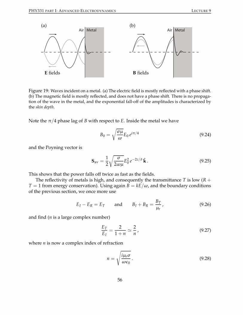
PHY331 PART I: ADVANCED ELECTRODYNAMICS LECTURE 9
Air Metal Air Metal(a) (b)
E fields B fields
Figure 19: Waves incident on a metal. (a) The electric field is mostly reflectedwith a phase shift.(b) The magnetic field is mostly reflected, and does not have a phase shift. There is no propaga-tion of the wave in the metal, and the exponential fall-off of the amplitudes is characterized bythe skin depth.
Note the π/4 phase lag of B with respect to E. Inside the metal we have
B0 =
√
σµ
ωE0 e
iπ/4 (9.24)
and the Poyning vector is
Sav =1
2
√
σ
2ωµE20 e
−2z/δ k . (9.25)
This shows that the power falls off twice as fast as the fields.The reflectivity of metals is high, and consequently the transmittance T is low (R+
T = 1 from energy conservation). Using again B = kE/ω, and the boundary conditionsof the previous section, we once more use
EI − ER = ET and BI + BR =BTµr, (9.26)
and find (n is a large complex number)
ETEI
=2
1+ n≃ 2n, (9.27)
where n is now a complex index of refraction
n =
√
iµrσ
ωǫ0. (9.28)
56
PHY331 PART I: ADVANCED ELECTRODYNAMICS LECTURE 9
In addition, we can solve Eq. (9.26) for the magnetic induction, which yields
BTBI
=2
1+ 1/n≃ 2 . (9.29)
The ratio of the Poynting vectors for the transmitted and incident waves is therefore
STSI
= Re4
n. (9.30)
This leads to the transmittance
T =
√
8ωǫ0
σ. (9.31)
Usually, the transmitted waves will be absorbed completely unless the metal is suffi-ciently thin. Whenσ → ∞ such as in a superconductor, the transmittance drops to zeroand everything is reflected. That is why high quality cavities are made with supercon-ducting mirrors.
9.3 Waves in plasmas
Finally, consider a plasma in which the electrons are disassociated from the atomic nu-clei. When an electric field is applied the electrons accelerate. The current density J
therefore lags the electric field, and the phase happens to be eiπ/2 = i. The nuclei aremuch heavier than the electrons, so they do not accelerate as fast and make a negligablecontribution to the conductivity. We can find the velocity v of the electrons by integrat-ing F = ma = eE, where all vector quantities are in the z direction. Using the electrondensity Ne, the current density is
J = Nev = NeieE
ωm, (9.32)
and the conductivity is
σ =J
E=ie2N
ωm. (9.33)
We substitute this into our expression for the complex wave vector k
k = k0
√
1− e2N
ω2mǫ0= k0
√
1−(ωp
ω
)2, (9.34)
where we defined the plasma frequency
ωp =
√
e2N
mǫ0. (9.35)
57
PHY331 PART I: ADVANCED ELECTRODYNAMICS LECTURE 9
Clearly, when the frequency of the waveω is larger than the plasma frequency, k is realand the plasma acts as a dielectric. Whenω < ω)p the plasma acts as a conductor.The ionosphere of the Earth is a plasma, and consequently for low enough frequen-
cies (long wavelengths) it acts as a mirror. Since the earth is also a conductor, lowfrequency radio waves (AM) can bounce between the ionosphere and the Earth to reachmuch further than high frequency (FM) radiowaves. The plasma frequency of the iono-sphere is about 3 MHz.
Further reading
– R.H. Good, Classical Electromagnetism, Saunders College Publishing (1999): Ch. 16, pp390-412.
– J.D. Jackson, Classical Electrodynamics, Wiley (2003): Sec. 7.1-7.6, pp 295-319.
– R.P. Feynman, Lectures on Physics, volume II, Addison-Wesley (1964): Ch. 32 & 33.
– H.J. Pain, The Physics of Vibrations and Waves, Wiley (1983): Ch. 7, pp 187-218.
– J.R. Reitz, F.J. Milford, & R.W. Christy, Foundations of Electromagnetic Theory, fourth edition,Addison-Wesley (1993): Ch. 17, pp 412-440.
– J. Schwinger, L.L. DeRaad, K.A.Milton, &W. Tsai, Classical Electrodynamics, The AdvancedBook Program, Westview Press (1998): Ch. 41-42, pp 427-448.
Exercises
1. Calculate the skin depth of copper for 60 Hz, 10 kHz, and 10 MHz. The conduc-tivity of copper is 5.8 · 107 Ω−1m.
2. Calculate the speed of a 1 MHz wave in copper and in glass.
58
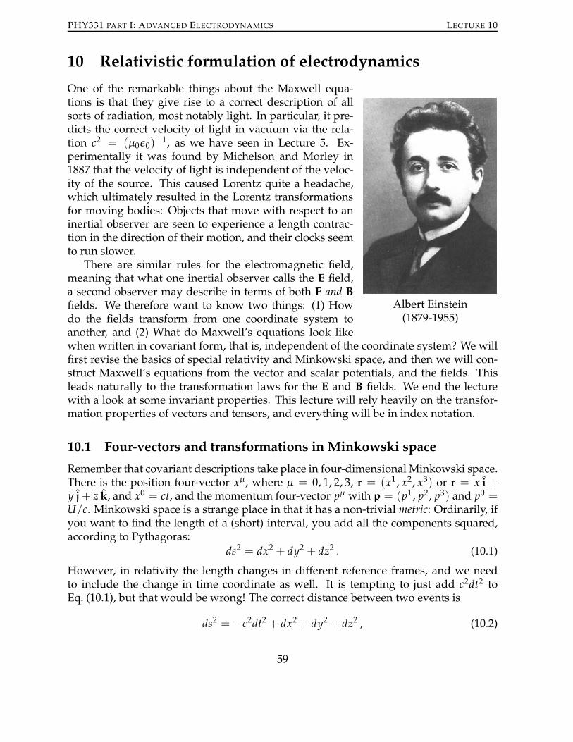
PHY331 PART I: ADVANCED ELECTRODYNAMICS LECTURE 10
10 Relativistic formulation of electrodynamics
Albert Einstein(1879-1955)
One of the remarkable things about the Maxwell equa-tions is that they give rise to a correct description of allsorts of radiation, most notably light. In particular, it pre-dicts the correct velocity of light in vacuum via the rela-tion c2 = (µ0ǫ0)
−1, as we have seen in Lecture 5. Ex-perimentally it was found by Michelson and Morley in1887 that the velocity of light is independent of the veloc-ity of the source. This caused Lorentz quite a headache,which ultimately resulted in the Lorentz transformationsfor moving bodies: Objects that move with respect to aninertial observer are seen to experience a length contrac-tion in the direction of their motion, and their clocks seemto run slower.There are similar rules for the electromagnetic field,
meaning that what one inertial observer calls the E field,a second observer may describe in terms of both E and Bfields. We therefore want to know two things: (1) Howdo the fields transform from one coordinate system toanother, and (2) What do Maxwell’s equations look likewhen written in covariant form, that is, independent of the coordinate system? We willfirst revise the basics of special relativity and Minkowski space, and then we will con-struct Maxwell’s equations from the vector and scalar potentials, and the fields. Thisleads naturally to the transformation laws for the E and B fields. We end the lecturewith a look at some invariant properties. This lecture will rely heavily on the transfor-mation properties of vectors and tensors, and everything will be in index notation.
10.1 Four-vectors and transformations in Minkowski space
Remember that covariant descriptions take place in four-dimensional Minkowski space.There is the position four-vector xµ, where µ = 0, 1, 2, 3, r = (x1, x2, x3) or r = x i+y j+ z k, and x0 = ct, and the momentum four-vector pµ with p = (p1 , p2, p3) and p0 =U/c. Minkowski space is a strange place in that it has a non-trivial metric: Ordinarily, ifyou want to find the length of a (short) interval, you add all the components squared,according to Pythagoras:
ds2 = dx2 + dy2 + dz2 . (10.1)
However, in relativity the length changes in different reference frames, and we needto include the change in time coordinate as well. It is tempting to just add c2dt2 toEq. (10.1), but that would be wrong! The correct distance between two events is
ds2 = −c2dt2 + dx2 + dy2 + dz2 , (10.2)
59

PHY331 PART I: ADVANCED ELECTRODYNAMICS LECTURE 10
with a minus sign in front of c2dt2! This is the definition of the distance in Minkowskispace, andwe can rewrite this as a vector equation (and also using Einstein’s summationconvention):
ds2 = (ct, x, y, z)
−1 0 0 00 1 0 00 0 1 00 0 0 1
ctxyz
≡ xµgµνxν = xµxµ = xµx
µ , (10.3)
where the four-vector xµ can be written as (ct, x, y, z). Notice that the matrix gµν has a“−1” on the diagonal, which is responsible for the minus sign in the metric. You alsosee that there is a difference between upper and lower indices. The four-vectors withupper indices are called contravariant, and the four-vectors with lower indices are calledcovariant. You can verify from Eq. (10.3) that the covariant four-vector has a relativeminus sign in the first component:
xµ = (−ct, x, y, z) . (10.4)
We are cheating a bit here, because the xµ on the left is a component, while the quantityon the right is a proper vector. However, this expression is to emphasize the effect of thevertical position of the index; it is not a proper equation. As you can see from Eq. (10.3),the metric raises or lowers the index, and gµν = gµν in the case of special relativity.We now amend the Einstein summation convention: the sum is implied over two re-
peating indices, one of which is upper, and the other is lower (convince yourself that thisdistinction is important). Carrying out the sum is called contraction. We can constructinvariant quantities (scalars) by contracting contravariant four-vectors with covariantfour-vectors. In general we write the components of a four-vector aµ as (a0 , a1 , a2, a3),and we have:
aµbµ = aµgµνbν = ∑
µ,ν
aµgµνbν
= −a0b0 +3
∑j=1
a jb j = −a0b0 + a · b , (10.5)
where greek indices sum over all four components, while roman indices sum only overthe spatial part5.As an example, let’s look at the four-momentum of a particle: p = (U/c, p1 , p2, p3),
and p2 = pµpµ can be written as p2 = −U2/c2 + |p|2. Since this is true for all inertialframes, it is true for the frame where the particle is at rest, so |p|2 = 0. Using U = mc2
with m the rest mass of the particle, we find p2 = −m2c2 (yes, in Minkowski space5You should be aware of the fact that the metric gµν can also be written as a diagonal matrix with
three −1 entries for the spatial part and one +1 for the temporal part. This does not lead to observabledifferences in the theory, so it is a convention. Unfortunately, both conventions are used regularly, somake sure you know what the metric is before you copy a relativistic formula from a book!
60
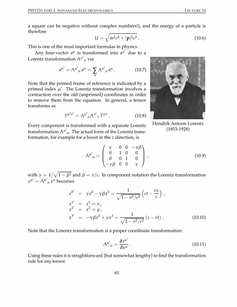
PHY331 PART I: ADVANCED ELECTRODYNAMICS LECTURE 10
a square can be negative without complex numbers!), and the energy of a particle istherefore
U =√
m2c4 + |p|2c2 . (10.6)
This is one of the most important formulas in physics.
Hendrik Antoon Lorentz(1853-1928)
Any four-vector aµ is transformed into aµ′due to a
Lorentz transformation Λµ′µ via
aµ′= Λµ′
µ aµ = ∑
µ
Λµ′µ a
µ . (10.7)
Note that the primed frame of reference is indicated by aprimed index µ′. The Lorentz transformation involves acontraction over the old (unprimed) coordinates in orderto remove them from the equation. In general, a tensortransforms as
Tµ′ν′= Λµ′
µΛν′ν T
µν . (10.8)
Every component is transformed with a separate Lorentz
transformation Λµ′µ . The actual form of the Lorentz trans-
formation, for example for a boost in the z direction, is
Λµ′µ =
γ 0 0 −γβ
0 1 0 00 0 1 0
−γβ 0 0 γ
, (10.9)
with γ = 1/√
1−β2 and β = v/c. In component notation the Lorentz transformation
xµ′= Λµ′
µ xµ becomes
x0′
= γx0 − γβx3 =1
√
1− v2/c2(
ct− vzc
)
,
x1′
= x1 = x ,x2
′= x2 = y ,
x3′
= −γβx0 + γx3 =1
√
1− v2/c2(z− vt) . (10.10)
Note that the Lorentz transformation is a proper coordinate transformation:
Λµ′µ =
∂xµ′
∂xµ. (10.11)
Using these rules it is straghtforward (but somewhat lengthy) to find the transformationrule for any tensor.
61

PHY331 PART I: ADVANCED ELECTRODYNAMICS LECTURE 10
10.2 Covariant Maxwell equations
Just like the position and momentum four-vectors, we would like to construct elec-tric and magnetic four-vectors. Unfortunately, it is not that simple: There are six fieldcomponents (three for E and three for B), and we cannot force them into four-vectors.On the other hand, we can combine the vector potential and the scalar potential into afourvector Aµ :
Aµ(x) =
(
Φ(x)
c,A(x)
)
, (10.12)
where x is again the position four-vector. The second four-vector that we can constructstraight away is the current density jµ :
jµ(x) =(
cρ(x), J(x))
. (10.13)
Since the Maxwell equations are differential equations, we also need to construct afour-vector out of the differential operators. Again, they come in two variations, covari-ant ∂µ and contravariant ∂µ :
∂µ =∂
∂xµ=
(
−1c
∂∂t,∇)
and ∂µ =∂
∂xµ=
(
1
c
∂∂t,∇)
. (10.14)
These operators transform just like ordinary vectors (but note the vertical position ofthe indices). We can construct an invariant with these operators if we contract them:
∂µ∂µ = ∂2x + ∂2y + ∂2z −1
c2∂2t = . (10.15)
This is the d’Alembertian, which we first encountered in lecture 3.The continuity equation (conservation of charge) then becomes particularly com-
pact:∂µ j
µ = 0 . (10.16)
Compare this with Eq. (2.19); the two equations say exactly the same thing! TheMaxwellequations in Eqs. (3.9) can be written as
∂µ∂µAν = µ0 jν (10.17)
Often people say that this encompasses all of electrodynamics. However, you shouldremember that we also need to know how charges respond to the fields, that is, weneed to know the Lorentz force. Since this force depends explicitly on the velocity ofthe particle, it is not in covariant form. Wewill consider the covariant Lorentz force later.We also see explicitly that the Maxwell equations are already relativistically correct: Wedid not change anything in Eqs. (3.9), we just rewrote everything. The compactness ofEq. (10.17) indicates that Lorentz invariance is a symmetry of electrodynamics (The moresymmetric the object, the more compact we can make its description: For example,
62

PHY331 PART I: ADVANCED ELECTRODYNAMICS LECTURE 10
compare the description of a perfect sphere with the description of a sponge). Lorentzinvariance is an important symmetry in quantum field theory and the standard model.Maxwell thought that the electric fields were carried by some substance that per-
vades all space, called the æther. Such a substance defines a natural reference frame,which would break Lorentz invariance. It was Einstein who disposed of the æther andmade all inertial reference frames equivalent. Thus he uncovered that electrodynamicswas a relativistic theory all along. In fact, his famous paper of 1905 on special relativitywas titled “On the electrodynamics of moving bodies”.In addition to the Maxwell equations in Eq. (10.17), we need to specify a particular
gauge for the four-vector potential Aµ if we actually want to calculate anything. Therelativistically invariant gauge is the Lorenz gauge
∂µAµ = 0 . (10.18)
Now that we have constructed the four-vector potential for the electromagnetic field,we can ask what the E and B fields look like in a relativistic setting. We can use therelations
E = −∇Φ− ∂A∂t
and B = ∇×A . (10.19)
If we write out a few components we get, for example,
Ex = −∂Φ
∂x− ∂Ax
∂t= −c
(
∂1A0 − ∂0A1)
,
Bx =∂Az∂y
− ∂Ay∂z
= −(∂2A3 − ∂3A2) . (10.20)
Obviously we can only fit all six components of the electric andmagnetic field into a rel-ativistic object if we have something with two indices. We call this the (anti-symmetric)field-strength tensor F:
Fµν = ∂µAν − ∂νAµ =
0 Ex/c Ey/c Ez/c−Ex/c 0 −Bz By−Ey/c Bz 0 −Bx−Ez/c −By Bx 0
. (10.21)
The relativistic transformation of the fields then becomes
Fµ′ν′
= Λµ′µΛν′
ν Fµν . (10.22)
For a boost v in the z direction given by Eq. (10.9) we find
E′x = γ(
Ex + vBy)
, E′y = γ(
Ey − vBx)
, E′z = Ez (10.23)
B′x = γ(
Bx −v
c2Ey
)
, B′y = γ(
By +v
c2Ex
)
, B′z = Bz . (10.24)
63
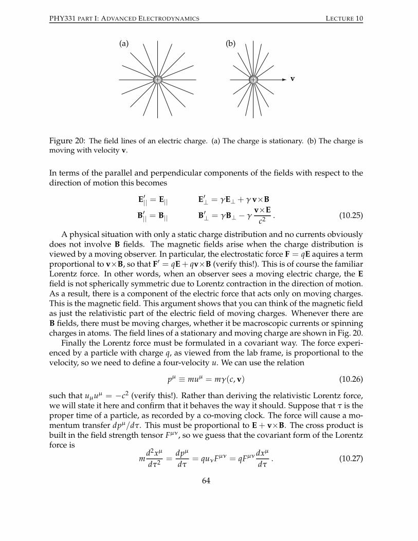
PHY331 PART I: ADVANCED ELECTRODYNAMICS LECTURE 10
+ +
(a) (b)
v
Figure 20: The field lines of an electric charge. (a) The charge is stationary. (b) The charge ismoving with velocity v.
In terms of the parallel and perpendicular components of the fields with respect to thedirection of motion this becomes
E′|| = E|| E′⊥ = γE⊥ + γ v×B
B′|| = B|| B′⊥ = γB⊥ − γv×Ec2. (10.25)
A physical situation with only a static charge distribution and no currents obviouslydoes not involve B fields. The magnetic fields arise when the charge distribution isviewed by a moving observer. In particular, the electrostatic force F = qE aquires a termproportional to v×B, so that F′ = qE+ qv×B (verify this!). This is of course the familiarLorentz force. In other words, when an observer sees a moving electric charge, the Efield is not spherically symmetric due to Lorentz contraction in the direction of motion.As a result, there is a component of the electric force that acts only on moving charges.This is the magnetic field. This argument shows that you can think of the magnetic fieldas just the relativistic part of the electric field of moving charges. Whenever there areB fields, there must be moving charges, whether it be macroscopic currents or spinningcharges in atoms. The field lines of a stationary andmoving charge are shown in Fig. 20.Finally the Lorentz force must be formulated in a covariant way. The force experi-
enced by a particle with charge q, as viewed from the lab frame, is proportional to thevelocity, so we need to define a four-velocity u. We can use the relation
pµ ≡ muµ = mγ(c, v) (10.26)
such that uµuµ = −c2 (verify this!). Rather than deriving the relativistic Lorentz force,
we will state it here and confirm that it behaves the way it should. Suppose that τ is theproper time of a particle, as recorded by a co-moving clock. The force will cause a mo-mentum transfer dpµ/dτ . This must be proportional to E+ v×B. The cross product isbuilt in the field strength tensor Fµν , so we guess that the covariant form of the Lorentzforce is
md2xµ
dτ2=dpµ
dτ= quνF
µν = qFµν dxµ
dτ. (10.27)
64

PHY331 PART I: ADVANCED ELECTRODYNAMICS LECTURE 10
These are the equations of motion for a relativistic particle in an electromagnetic field.Let’s see what the different components of f look like:
fx =dp1
dτ= qF1νuν = γq
(
cExc
+ vx · 0+ vyBz − vzBy)
fy =dp2
dτ= qF2νuν = γq
(
cEy
c− vxBz + vy · 0+ vzBx
)
fz =dp3
dτ= qF3νuν = γq
(
cExc
+ vxBy − vyBx − vz · 0)
(10.28)
These are indeed the three components of the Lorentz force, with an extra factor γ. Thisis correct, because the term dpµ/dτ also has an implicit γ factor in the relativistic mass.Remains the question of what is ft:
c ft = cdp0
dτ= qcF0νuν = γq
(
vx · Ex + vyEy + vzEz)
= γq v · E . (10.29)
This is the relativistic work done on the particle by the fields. So you see that it all worksout.
10.3 Invariant quantities
When the fields and potentials change when viewed in different inertial frames, it isimportant to know what the invariant quantities of a theory are. These quantities arethe same in all reference frames, so you can evaluate them in whichever frame makesthe calculation easiest. There are many invariants, most notably the magnitude of four-vectors a2 = aµaµ . You can use the differential operator as well in the construction ofinvariants (see Eq. (10.13) for an important example). A quantity is invariant when itdoes not depend on the coordinates, so in index notation the quantity has no indices.The quantity 14FµνF
µν is invariant (why?), and can be evaluated as
1
4FµνF
µν =1
4gρµgσνF
ρσFµν =B2
2− E
2
2c2. (10.30)
This is the Lagrangian (density) of the electromagnetic field, which plays a pivotal rolein particle physics.We can also construct the dual of the field-strength tensor
Fµν =1
2ǫµνρσFρσ =
0 −Bx −By −BzBx 0 Ez/c −Ey/cBy −Ez/c 0 Ex/cBz Ey/c −Ex/c 0
. (10.31)
which is a pseudo-tensor. Here we used the Levi-Civita (pseudo) tensor ǫµνρσ , whichreturns 1 if the indices make an even permutation,−1 if they make an odd permutation,
65

PHY331 PART I: ADVANCED ELECTRODYNAMICS LECTURE
and 0 otherwise. The invariant product FµνFµν is
FµνFµν = 4E · B/c . (10.32)
Finally, the microscopic Maxwell equations can be written in terms of the fields as
∂µFµν = µ0 j
ν and ∂µFµν = 0 (10.33)
Further reading
– R.H. Good, Classical Electromagnetism, Saunders College Publishing (1999): Ch. 18, pp430-490.
– J.D. Jackson, Classical Electrodynamics, Wiley (1998): Ch. 11, pp 514-566.
– R.P. Feynman, Lectures on Physics, volume II, Addison-Wesley (1964): Ch. 25, 26 & 31.
– J.R. Reitz, F.J. Milford, & R.W. Christy, Foundations of Electromagnetic Theory, fourth edition,Addison-Wesley (1993): Ch. 22, pp 558-578.
– C.A. Brau, Modern Problems in Classical Electrodynamics, Oxford University Press (2004):Ch. 1, pp 29-72.
– J. Schwinger, L.L. DeRaad, K.A.Milton, &W. Tsai, Classical Electrodynamics, The AdvancedBook Program, Westview Press (1998): Ch. 10, pp 111-124.
Exercises
1. Calculate the determinant of the Lorentz transformation Λµ′µ in Eq. (10.9)
2. Calculate the expression for the energy of a relativistic particle as in Eq. (10.6), butnow with the metric
gµν =
1 0 0 00 −1 0 00 0 −1 00 0 0 −1
.
3. Show that gµν is a proper transformation that can be written as
gµν =∂xµ∂xν.
4. Prove that E · B is Lorentz invariant.
5. Show that the phase of an electromagnetic wave is a Lorentz invariant quantity.What exactly is invariant here?
6. Calculate Fµν , FµνFµν , Fµν , and verify Eq. (10.32).
66

PHY331 PART I: ADVANCED ELECTRODYNAMICS LECTURE A
A Special coordinates and vector identities
A.1 Coordinate systems
Often it is much more convenient to use cylindrical or spherical coordinates, ratherthan cartesian coordinates. The differential operators change accordingly. For cartesiancoordinates:
A×B = (AyBz − AzBy)x+ (AzBx − AxBz)y+ (AxBy − AyBx)z (A.1)
∇ f =∂ f∂xx+
∂ f∂yy+
∂ f∂zz (A.2)
∇ ·A =∂Ax∂x
+∂Ay∂y
+∂Az∂z
(A.3)
∇×A =
(
∂Az∂y
− ∂Ay∂z
)
x+
(
∂Ax∂z
− ∂Az∂x
)
y+
(
∂Ay∂x
− ∂Ax∂y
)
z (A.4)
Cylindrical coordinates:
∇ f =∂ f∂ρ
ρ +1
ρ
∂ f∂φ
φ +∂ f∂zz (A.5)
∇ ·A =1
ρ
∂(ρAρ)
∂ρ+1
ρ
∂Aφ
∂φ+
∂Az∂z
(A.6)
∇×A =
(
1
ρ
∂Az∂φ
− ∂Aφ
∂z
)
ρ +
(
∂Aρ
∂z− ∂Az
∂ρ
)
φ +1
ρ
(
∂(ρAφ)
∂ρ− ∂Aρ
∂φ
)
z (A.7)
∇2 f =1
ρ
∂∂ρ
(
ρ∂ f∂ρ
)
+1
ρ2∂2 f∂φ2
+∂2 f∂z2
(A.8)
x
y
z
Figure 21: Cartesian coordinates (x, y, z).
67

PHY331 PART I: ADVANCED ELECTRODYNAMICS LECTURE A
x
y
z
φρ
Figure 22: Cylindrical coordinates (ρ,φ, z).
Spherical coordinates:
∇ f =∂ f∂rr+1
r
∂ f∂θ
θ +1
r sinθ
∂ f∂φ
φ (A.9)
∇ ·A =1
r2∂(r2Ar)
∂r+
1
r sinθ
∂(Aθ sinθ)
∂θ+
1
r sinθ
∂Aφ
∂φ(A.10)
∇×A =1
r sinθ
(
∂(Aφ sinθ)
∂θ− ∂Aθ
∂φ
)
r (A.11)
+1
r
(
1
sinθ
∂Ar∂φ
− ∂(rAφ)
∂r
)
θ (A.12)
+1
r
(
∂(rAθ)
∂r− ∂Ar
∂θ
)
φ (A.13)
∇2 f =1
r2∂∂r
(
r2∂ f∂r
)
+1
r2 sinθ
∂∂θ
(
sinθ∂ f∂θ
)
+1
r2 sin2θ
∂2 f∂φ2
(A.14)
x
y
z
φ
r
θ
Figure 23: Spherical coordinates (r,φ,θ).
68

PHY331 PART I: ADVANCED ELECTRODYNAMICS LECTURE A
A.2 Integral theorems and vector identities
Having defined the divergence and the curl of vector fields, we can state the importantintegral theorems (without proof):
∫
V∇ ·A dV =
∮
SA · dS (Gauss’ theorem) (A.15)
∫
S(∇×A) · dS =
∮
CA · dl (Stokes’ theorem) (A.16)
∫ b
a∇ f · dl = f (b) − f (a) (A.17)
∫
V
(
f∇2g− g∇2 f)
dV =∮
S( f∇g− g∇ f ) · dS (Green’s theorem) (A.18)
and some important vector identities, such as relations between 3-vectors:
A · (B×C) = B · (C×A) = C · (A×B) (A.19)
A×(B×C) = (A ·C)B− (A · B)C (A.20)
(A×B) · (C×D) = (A ·C)(B ·D)− (A ·D)(B ·C) (A.21)
first derivatives:
∇ · (φA) = φ(∇ ·A) +A · (∇φ) (A.22)
∇×(φA) = φ(∇×A) + (∇φ)×A (A.23)
∇(A · B) = A×(∇×B) + B×(∇×A) + (A · ∇)B+ (B · ∇)A (A.24)
∇ · (A×B) = B · (∇×A)−A · (∇×B) (A.25)
∇×(A×B) = (B · ∇)A− (A · ∇)B+A(∇ · B)− B(∇ ·A) (A.26)
and second derivatives:
∇ · (∇×A) = 0 (A.27)
∇×(∇φ) = 0 (A.28)
∇×(∇×A) = ∇(∇ ·A)−∇2A (A.29)
A.3 Levi-Civita tensor
Finally, we may sometimes use the so-called Levi-Civita symbol ǫi jk, which returns avalue of 1 when (i jk) is an even permutation of the indices, −1 if (i jk) is an odd per-mutation, and 0 otherwise (for example when two indices are the same). It obeys theidentity
3
∑k=1
ǫi jkǫklm =3
∑k=1
ǫi jkǫlmk = δilδ jm − δimδ jl , (A.30)
where δi j is of course the Kronecker delta, which returns 1 if i = j and 0 if i 6= j.
69

PHY331 PART I: ADVANCED ELECTRODYNAMICS LECTURE B
B Unit systems in electrodynamics
Carl Friedrich Gauss(1777-1855)
Traditionally, electrodynamics is plagued by the use ofmany different sets of units. In these lecture notes weuse SI units (Systeme International) exclusively. However,many people also use Gaussian units, so it is worthwhileto spend some time exploring the difference betwen theseunits. In particular, you should be able to read the set ofunits used off the Maxwell equations. The rule of thumbis: if they involve factors of 4π , then they most likely useGaussian units.Carl Friedrich Gauss was a German mathematician
who in the 1830s did (among very many other things)worldwide measurements of the Earth’s magnetic field.Not only are the Gaussian units named after him, the unitof magnetic induction in Gaussian units is also called theGauss (G). In SI units the unit of magnetic induction isthe Tesla (T), after the Serbian inventor Nikola Tesla (1853-1943).There is a certain arbitrariness in Maxwell’s equations,
the Lorentz force, and the continuity equation, in the sense that we can add constantsk1, k2, . . . to the equations that affect only the units, and not the physics:
k1∇ · J+ ∂ρ
∂t= 0 and F = k2ρE+ k3J×B (B.1)
∇ · E = k4ρ and ∇ · B = 0 (B.2)
∇×E+ k5∂B∂t
= 0 and ∇×B = k6J+ k7∂E∂t
(B.3)
Not all the constants k1 to k7 are independent. Some manipulation of the above equa-tions will give the identity
k6∇ · J+ k4k7∂ρ
∂t= 0 (B.4)
so we have the restriction that k6 = k1k4k7. Similarly, by rederiving the wave equationswe find that k5k7 = c−2.More confusion arises when we consider macroscopic media. Gauss’ law in terms of
the polarization field becomes
∇ · (E+ k4P) = k4ρfree . (B.5)
which defines the displacement field
D = k8(E+ k4P) . (B.6)
70

PHY331 PART I: ADVANCED ELECTRODYNAMICS LECTURE B
Similarly, with a bound current density Jbound = ∇×M+ P the Maxwell-Ampere lawbecomes
∇×(B− k6M) = k6Jfree+ k7∂∂t
(E+ k4P) . (B.7)
The magnetic field is then defined as
H = k9(B− k6M) . (B.8)
The different constants k1 . . . k9 in both SI and Gaussian units are given by
k1 k2 k3 k4 k5 k6 k7 k8 k9SI units 1 1 1 ǫ−1
0 1 µ0 c−2 ǫ0 µ−10
Gaussian units 1 1 c−1 4π c−1 4πc−1 c−1 1 1
As you know, in the SI system the fundamental units are meter (m), kilogram (kg),second (s), and ampere (A). The unit of force is the Newton (N), which is of coursekg m/s2. Just like the second and the kilogram, the ampere is defined operationally.One ampere is the amount of current needed to create a force of 2 · 10−7 N per meterlength between two infinitely long parallel wires separated by a distance of one meter.In the Gaussian system, the fundamental units of mass, length, and time are the
gram (g), centimeter (cm), and again the second (s). Instead of the ampere, the otherfundamental unit is the statcoulomb (statC) for the unit of charge. The statvolt (statV)is the unit of potential, and obeys 1 statV = 1g cm/statC s2.
charge current E B µ0 ǫ0
SI C = As A N/C = V/m T = N/Am Tm/A C2/Nm2
Gauss statC statA = statC/s statV/cm G(statV/cm) – –
In Gaussian units the permittivity and the permeability are dimensionless.
Further reading
– W.J. Duffin, Electricity and Magnetism, McGraw-Hill (1990): App. C, pp 406-413.
– J.R. Reitz, F.J. Milford, & R.W. Christy, Foundations of Electromagnetic Theory, fourth edition,Addison-Wesley (1993): App. III, pp 599-602.
– C.A. Brau, Modern Problems in Classical Electrodynamics, Oxford University Press (2004):Appendix, pp 581-589.
– J. Schwinger, L.L. DeRaad, K.A.Milton, &W. Tsai, Classical Electrodynamics, The AdvancedBook Program, Westview Press (1998): App. A, pp 555-559.
71