photon mapping (pm), progressive pm, stochastic ppm jiří vorba
TRANSCRIPT
Photon Mapping (PM), Progressive PM,Stochastic PPM
Jiří Vorba

What are they used for?
• Methods for computing the Global Illumination(GI)
• GI = Direct + Indirect Illumination (multiple bounces)
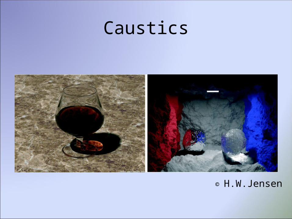
Caustics
© H.W.Jensen
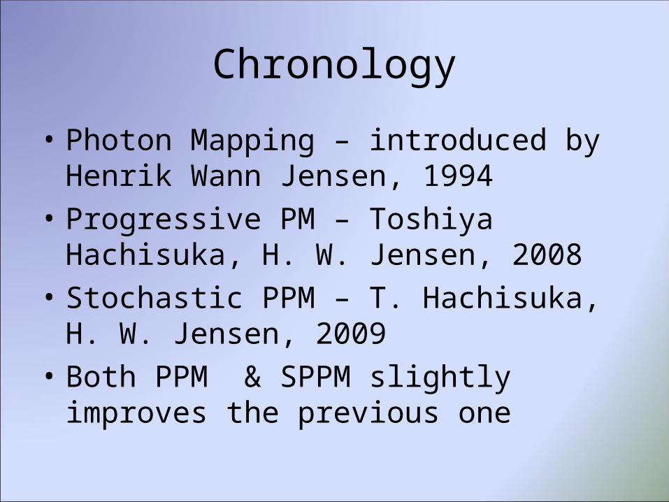
Chronology
• Photon Mapping – introduced by Henrik Wann Jensen, 1994
• Progressive PM – Toshiya Hachisuka, H. W. Jensen, 2008
• Stochastic PPM – T. Hachisuka, H. W. Jensen, 2009
• Both PPM & SPPM slightly improves the previous one

Photon Mapping - taxonomy
• Hybrid algorithm – combines “the best” of two worlds: – Radiosity – computes radiance (radiosity) values
for every mesh element (i.e. the object-space method)
– Ray-tracing – computes radiance values for every pixel by generating paths between the pixel and light sources

Photon Mapping – taxonomy II
• Multipass method – generally computing various parts of the light transport and then combining them together– special care needs to be take about not computing
the same light transport twice (too bright parts of the scene)
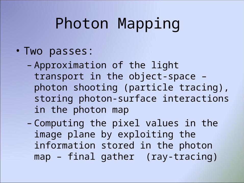
Photon Mapping
• Two passes:– Approximation of the light transport in the object-
space – photon shooting (particle tracing), storing photon-surface interactions in the photon map
– Computing the pixel values in the image plane by exploiting the information stored in the photon map – final gather (ray-tracing)
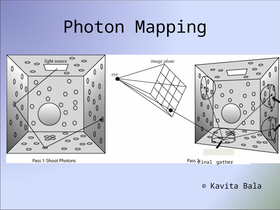
Photon Mapping
Final gather
© Kavita Bala
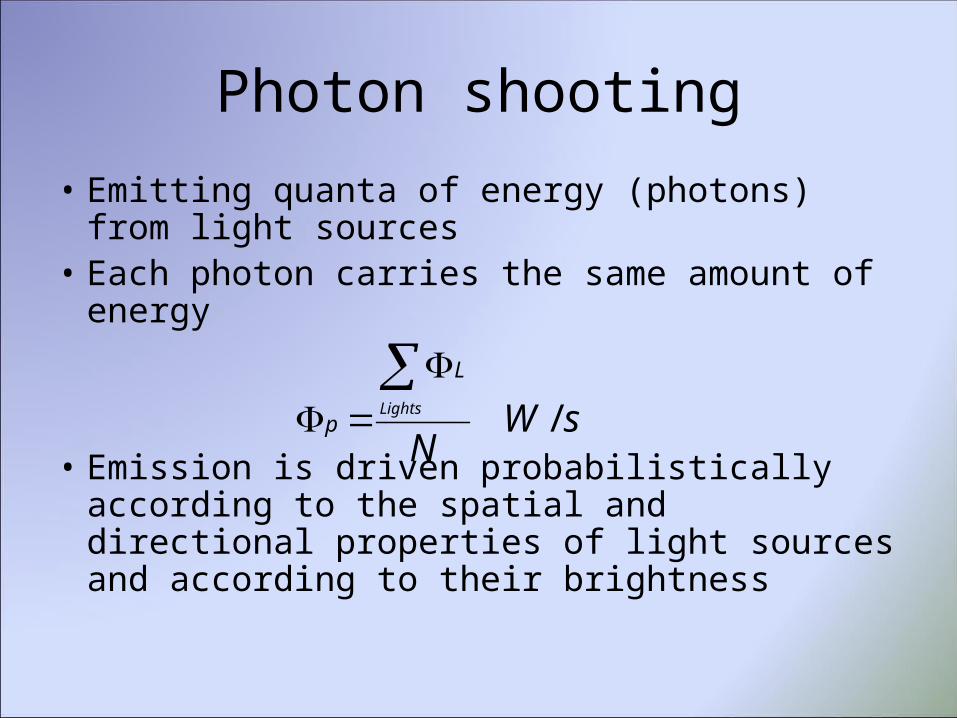
Photon shooting
• Emitting quanta of energy (photons) from light sources
• Each photon carries the same amount of energy
• Emission is driven probabilistically according to the spatial and directional properties of light sources and according to their brightness
sWN
Lights
L
p /
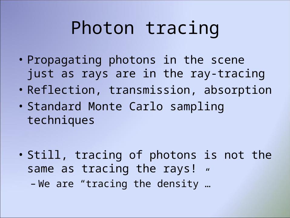
Photon tracing
• Propagating photons in the scene just as rays are in the ray-tracing
• Reflection, transmission, absorption• Standard Monte Carlo sampling techniques
• Still, tracing of photons is not the same as tracing the rays!– We are “tracing the density”…
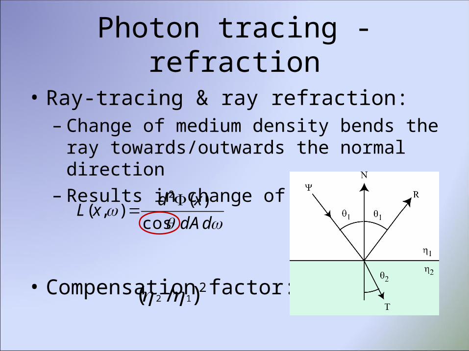
Photon tracing - refraction
• Ray-tracing & ray refraction:– Change of medium density bends the ray
towards/outwards the normal direction– Results in change of energy
• Compensation factor:2)/( 12
ddA
xdxL
cos
)(),(
2
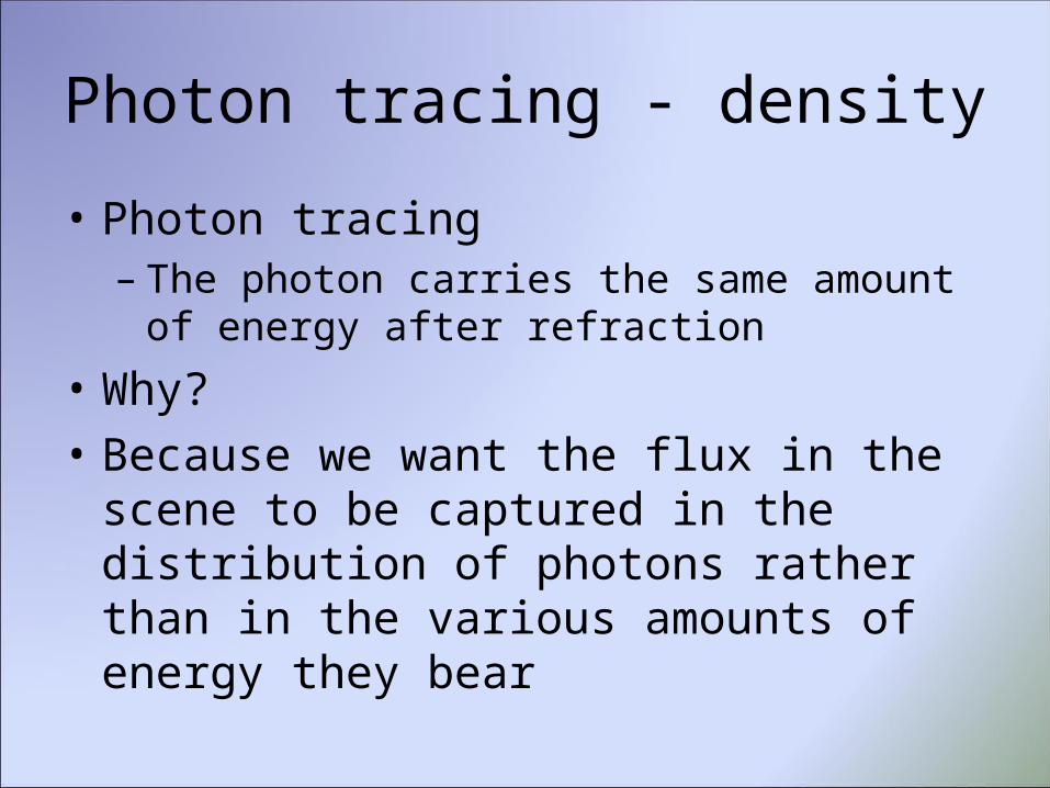
Photon tracing - density
• Photon tracing– The photon carries the same amount of energy
after refraction
• Why?• Because we want the flux in the scene to be
captured in the distribution of photons rather than in the various amounts of energy they bear

Photons approximates the radiosity
© Philippe Bekaert
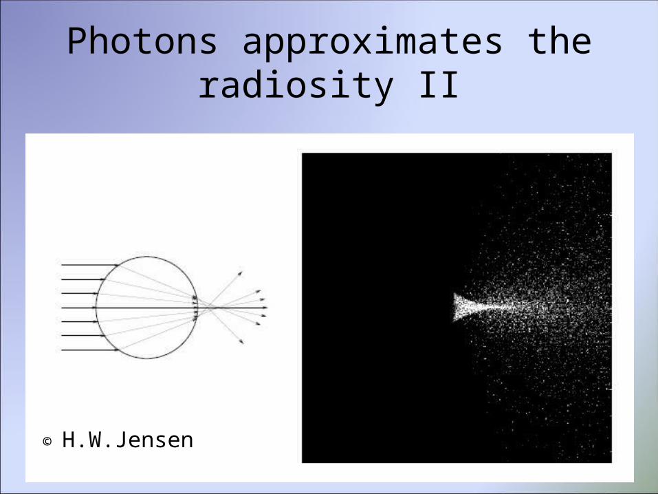
Photons approximates the radiosity II
© H.W.Jensen
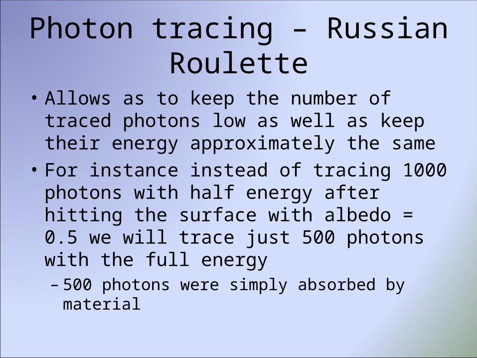
Photon tracing – Russian Roulette
• Allows as to keep the number of traced photons low as well as keep their energy approximately the same
• For instance instead of tracing 1000 photons with half energy after hitting the surface with albedo = 0.5 we will trace just 500 photons with the full energy– 500 photons were simply absorbed by material
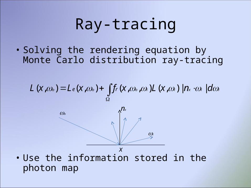
Ray-tracing
• Solving the rendering equation by Monte Carlo distribution ray-tracing
• Use the information stored in the photon map
iixiiooo dnxLxfxLxL re ||),(),,(),(),(
xn
x
o
i

Photon map query
• We can query the photon map about the estimate of the reflected radiance from any surface point
iixiiooo dnxLxfxLxL re ||),(),,(),(),(
),(),(),( ooo xLxLxL re
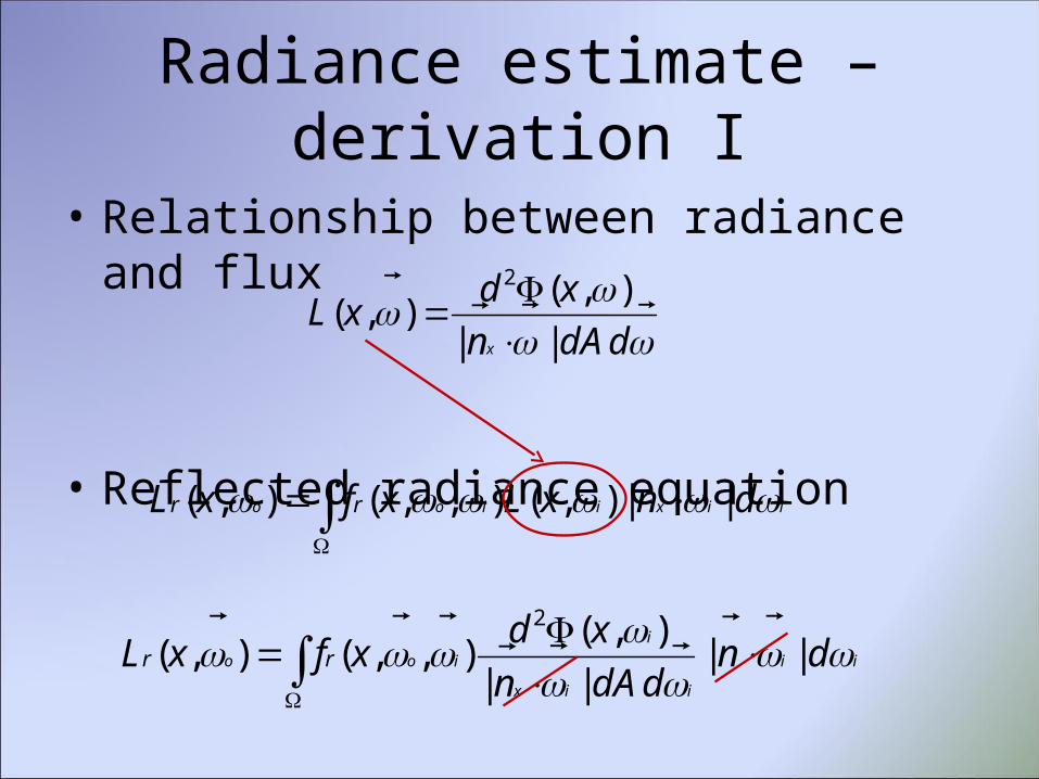
• Relationship between radiance and flux
• Reflected radiance equation
Radiance estimate – derivation I
iixiioo dnxLxfxL rr ||),(),,(),(
ddAn
xdxL
x ||
),(),(
2
ii
iix
i
ioo dnddAn
xdxfxL rr
||
||
),(),,(),(
2
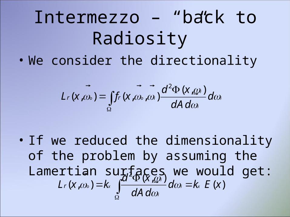
• We consider the directionality
• If we reduced the dimensionality of the problem by assuming the Lamertian surfaces we would get:
Intermezzo – “back to Radiosity”
i
i
i
ioo dddA
xdxfxL rr
),(),,(),(
2
)(),(
),(2
xEkdddA
xdkxL xi
i
i
xor
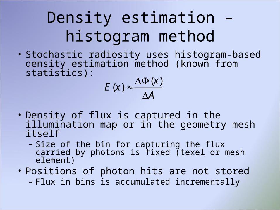
• Stochastic radiosity uses histogram-based density estimation method (known from statistics):
• Density of flux is captured in the illumination map or in the geometry mesh itself– Size of the bin for capturing the flux carried by
photons is fixed (texel or mesh element)• Positions of photon hits are not stored– Flux in bins is accumulated incrementally
Density estimation – histogram method
A
xxE
)(
)(
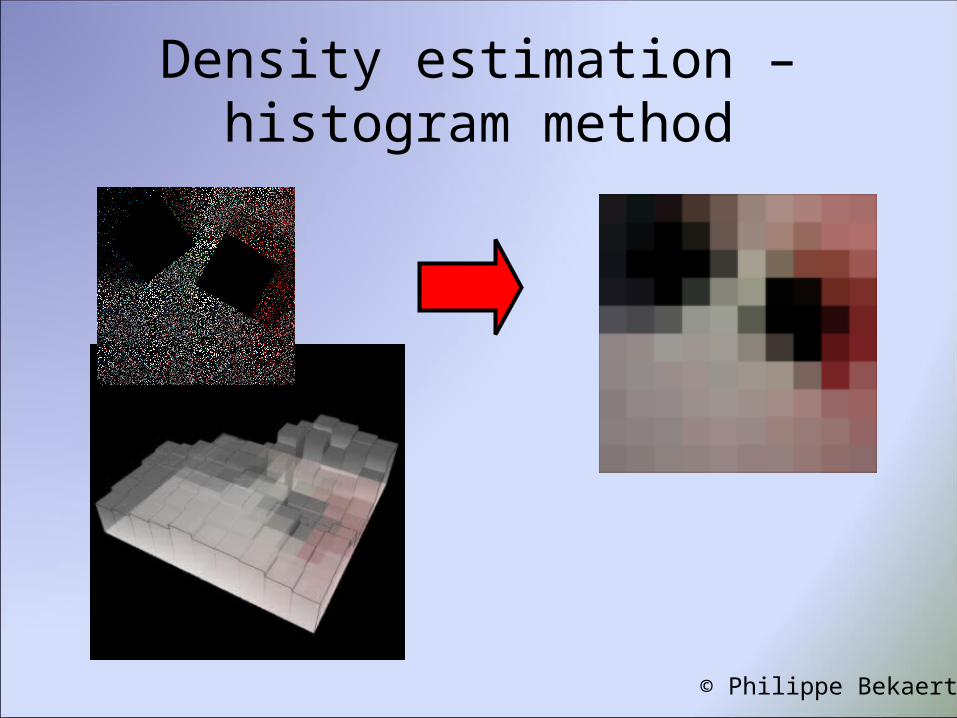
Density estimation – histogram method
© Philippe Bekaert

• What if we fixed the number of photons in density estimation (N/A) instead of fixing the surface area?
• Lets look for the N nearest photons• Density estimation is then determined by the
size of an area where we found thouse N photons
Density estimation – nearest neighbour
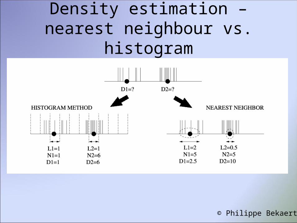
Density estimation – nearest neighbour vs. histogram
© Philippe Bekaert
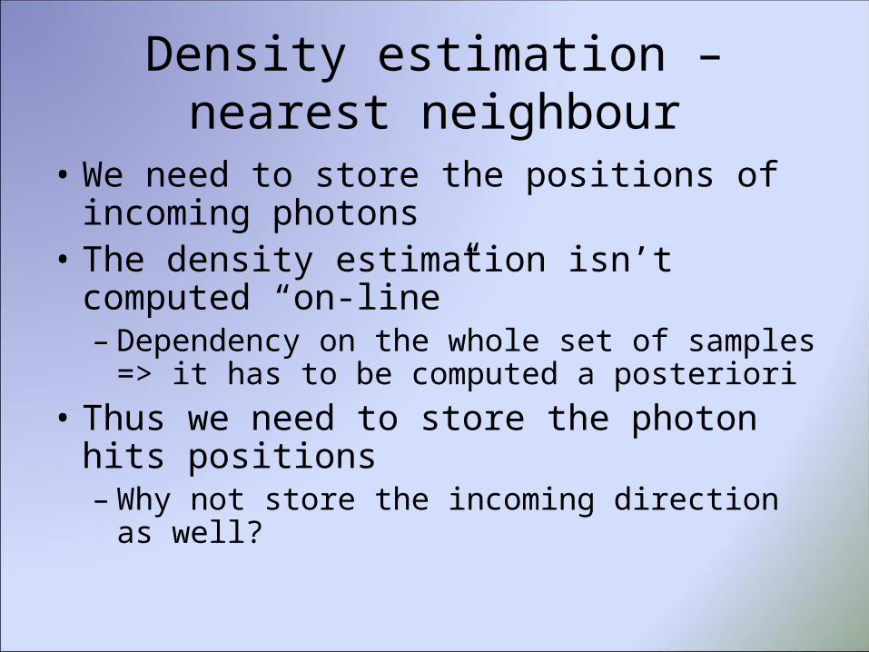
• We need to store the positions of incoming photons
• The density estimation isn’t computed “on-line”– Dependency on the whole set of samples => it has
to be computed a posteriori• Thus we need to store the photon hits
positions– Why not store the incoming direction as well?
Density estimation – nearest neighbour

• Photon map stores information about1. Photons hit positions2. Incoming photon direction3. Flux carried by the photon
Radiance estimation – derivation II
i
i
i
ioo dddA
xdxfxL rr
),(),,(),(
2

• Apply the nearest neighbour density estimation & multiply the samples by their flux and BRDF
• Assume that each photon in searched space ΔA hits the surface right at x:
• Photons look up can be imagined as expanding the sphere around x until it contains n photons
• Lets suppose that the area around the x is locally flat:
Radiance estimation – derivation III
n
p
rrA
xxfxL
p
poo
1
),(),,(),(
n
p
rr ppoo xxfr
xL1
2),(),,(
1),(
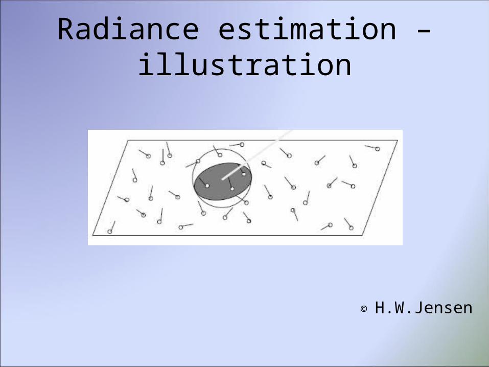
Radiance estimation – illustration
© H.W.Jensen
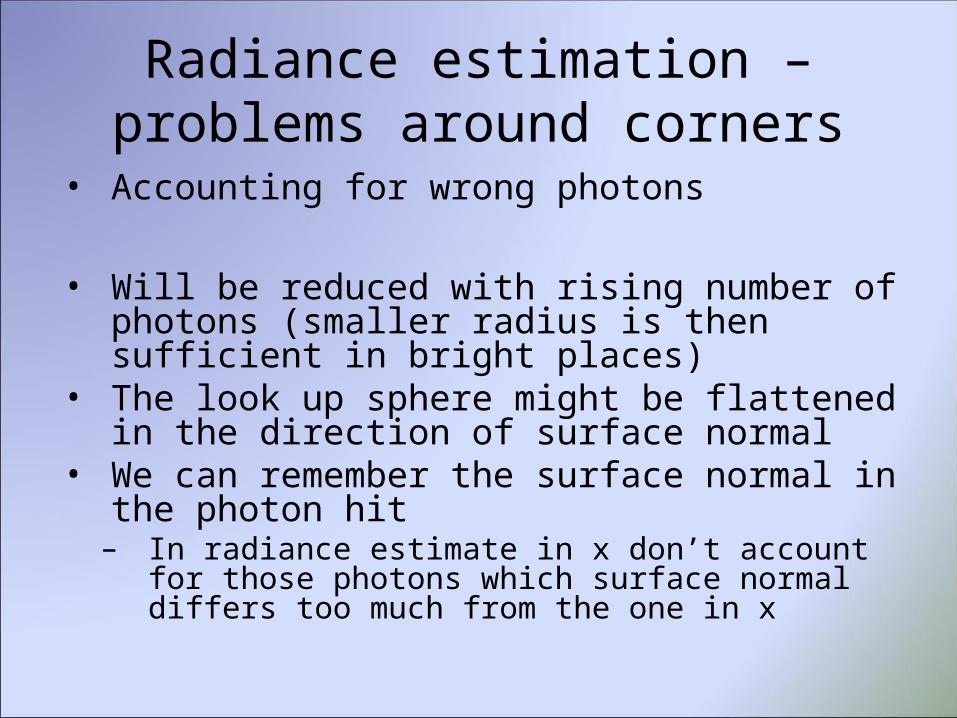
Radiance estimation – problems around corners
• Accounting for wrong photons
• Will be reduced with rising number of photons (smaller radius is then sufficient in bright places)
• The look up sphere might be flattened in the direction of surface normal
• We can remember the surface normal in the photon hit– In radiance estimate in x don’t account for those
photons which surface normal differs too much from the one in x

Radiance estimation – problems around corners
© H.W.Jensen

Radiance estimation – problems close to the walls
• obrazek
• Disk or sphere projection to locally flat surface may yield the wrong area estimate
• Solutions:– Computing the convex hull of accounted photons– Or better: use the kernel-density estimation
technique instead of nearest-neighbour (simply just filtering the radiance estimate by weighting the samples)
©
H.W.Jensen

Direct visualization of photon map (ray- casting on diffuse surfaces)
© H.W.Jensen
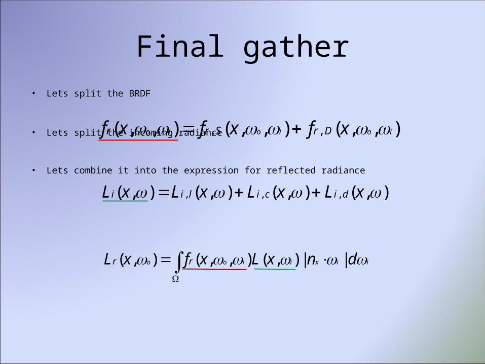
Final gather• Lets split the BRDF
• Lets split the incoming radiance
• Lets combine it into the expression for reflected radiance
),(),(),(),( ,,,
xLxLxLxL dicilii
),,(),,(),,( ,, ioioio xfxfxf DrSrr
iixiioo dnxLxfxL rr ||),(),,(),(

Reflected radiance equation
iixiioo dnxLxfxL rr ||),(),,(),(
ininxinliino dnxLxfr ||),(),,( ,
ininxindiinciino dnxLxLxf Sr ||)),(),()(,,( ,,,
ininxinciino dnxLxf Dr ||),(),,( ,,
ininxindiino dnxLxf Dr ||),(),,( ,,
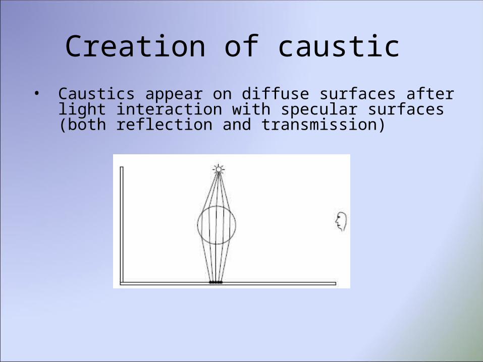
Creation of caustic • Caustics appear on diffuse surfaces after light interaction
with specular surfaces (both reflection and transmission)
More photon maps• Create the special photon map for caustic photons– Trace them separately (store the photon on the first non-specular surface -> S+D paths)– Cast photons only against specular surfaces – light source projection maps
• Create the special photon map for indirect illumination• Create the special photon map for participating media effects (behind the scope
of the talk)
Final gather II
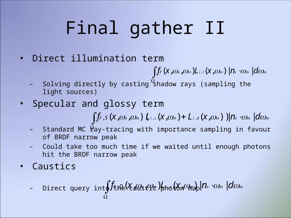
• Direct illumination term
– Solving directly by casting shadow rays (sampling the light sources)
• Specular and glossy term
– Standard MC ray-tracing with importance sampling in favour of BRDF narrow peak
– Could take too much time if we waited until enough photons hit the BRDF narrow peak
• Caustics
– Direct query into the caustic photon map
ininxinliino dnxLxfr ||),(),,( ,
ininxindiinciino dnxLxLxf Sr ||)),(),()(,,( ,,,
ininxinciino dnxLxf Dr ||),(),,( ,,

Final gather III
• Multiple diffuse reflections– Resulting illumination is very soft (caustics are in the other map – in
MC methods are caustics the biggest source of noice)– Thus we can use MC methods or classical Irradiance cashing methods
ininxindiino dnxLxf Dr ||),(),,( ,,

Different components of rendered solution
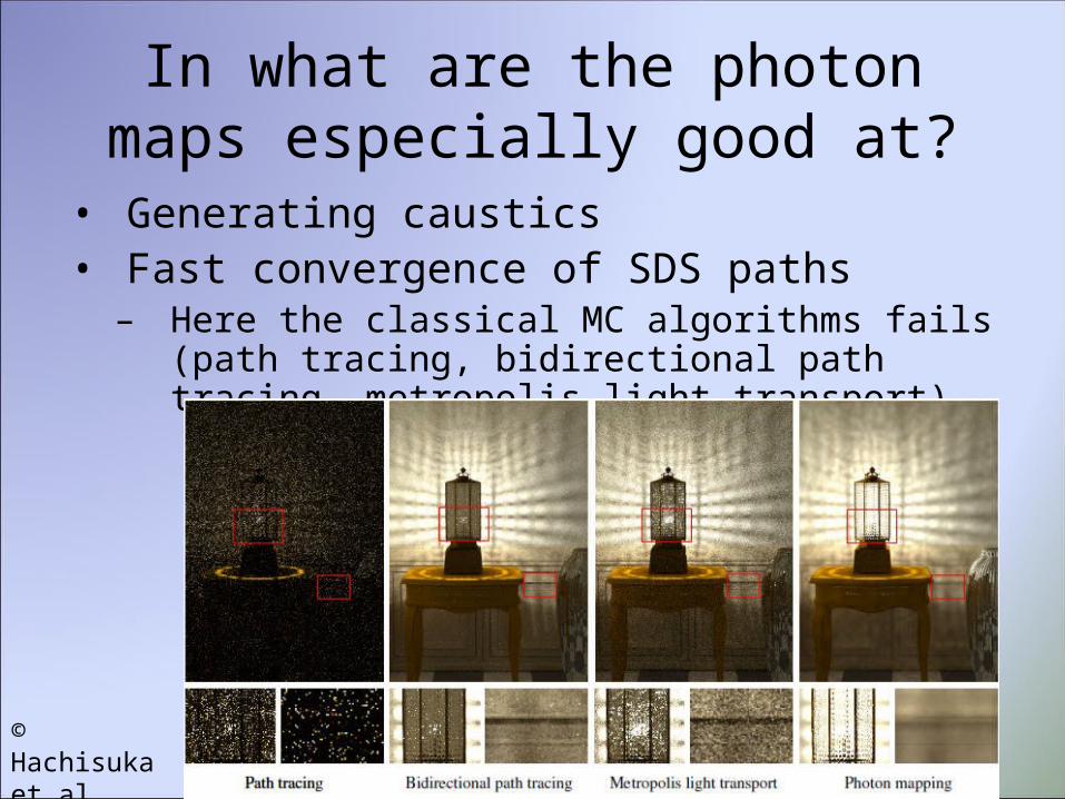
In what are the photon maps especially good at?
• Generating caustics• Fast convergence of SDS paths– Here the classical MC algorithms fails (path tracing,
bidirectional path tracing, metropolis light transport)
© Hachisuka et al.
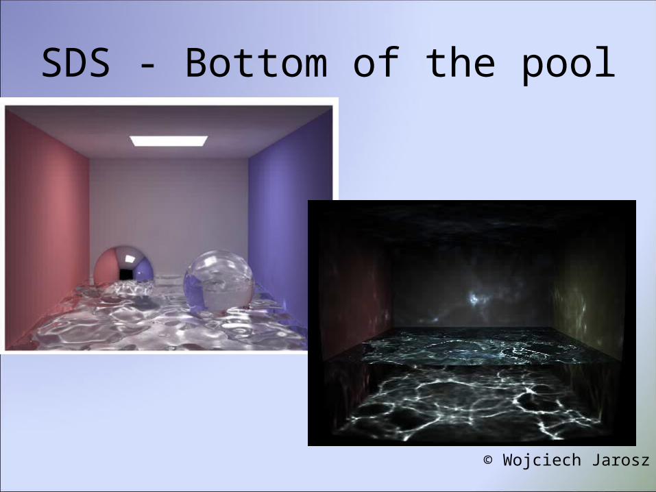
SDS - Bottom of the pool
© Wojciech Jarosz
Main disadvantages of PM
• Biased– Still, consistent
• Cannot get arbitrarily precise results– We are strictly limited by the physical memory boundary– Thus not suitable in the areas of predictive rendering
Progressive PM
Jiří Vorba
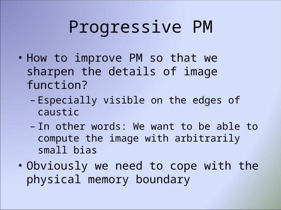
Progressive PM
• How to improve PM so that we sharpen the details of image function?– Especially visible on the edges of caustic– In other words: We want to be able to compute
the image with arbitrarily small bias
• Obviously we need to cope with the physical memory boundary

First idea
• Use the memory more times than one and combine the results from N photon maps
• Averaging radiance estimates– In the point x where we want to query PM we have N
radiance estimates– For averaging we need to use histogram-density
estimate method = fixing the radius; (remember histogram vs. nearest neighbour)
• It is not consistent– Getting smoother results but still blurry

Question
• How to combine illumination approximation from more photon maps so that we get in the final solution the results which are not present in any single photon map we have?– i.e. to have the consistent radiance estimate
combination

Second idea
• Says: “The algorithm of PM is consistent.”• So what?! Did it help us? We’ve already heard
that…• It gives us a clue how to do it– We have to progressively decrease the radius while
merging the results from multiple photon maps– More work has to be done to achieve the goal…
1,0),(),(),,(
1lim
12
oppo xLxxfr
r
N
p
rN
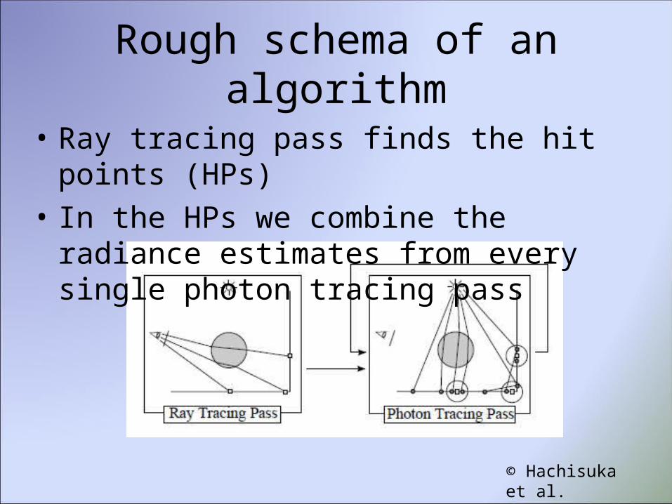
Rough schema of an algorithm
© Hachisuka et al.
• Ray tracing pass finds the hit points (HPs)• In the HPs we combine the radiance estimates
from every single photon tracing pass

Radius reduction• Main idea:– We suppose that the density d(x)=n/(πr2) around x is
invariant– Thus radius can be reduced if we reduce the number
of photons in the estimate• On the other hand to satisfy the condition of
consistency we need have gain of photons in the estimate
• Solution:– Lets keep just fraction of new photons after each
iteration
Radius reduction - derivation
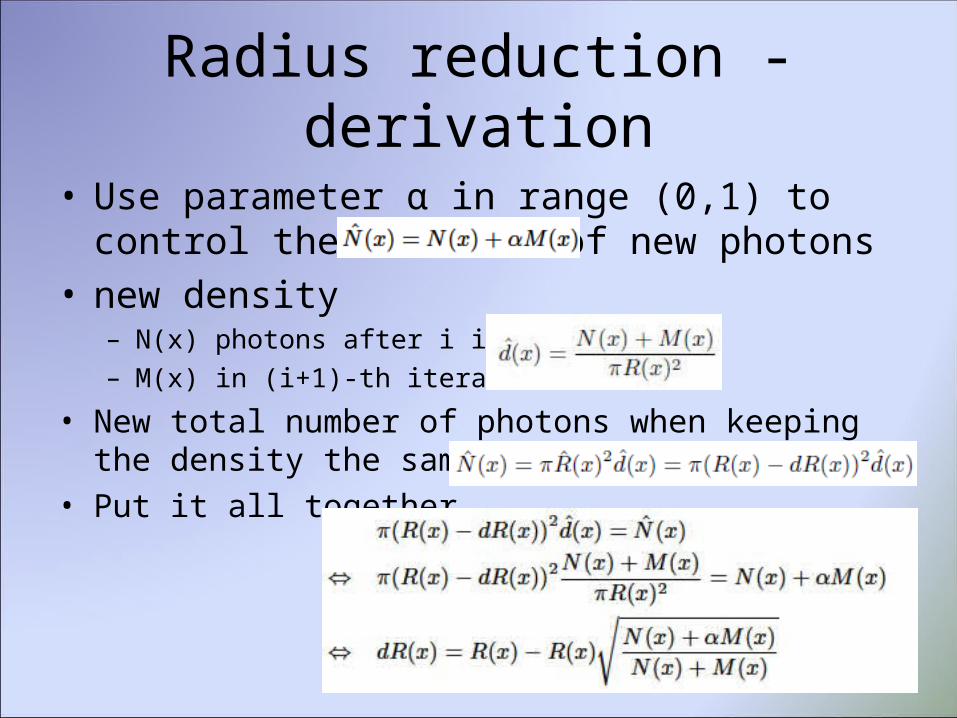
• Use parameter α in range (0,1) to control the fraction of new photons
• new density– N(x) photons after i iterations– M(x) in (i+1)-th iteration
• New total number of photons when keeping the density the same, just reducing radius
• Put it all together
Radius reduction - derivation
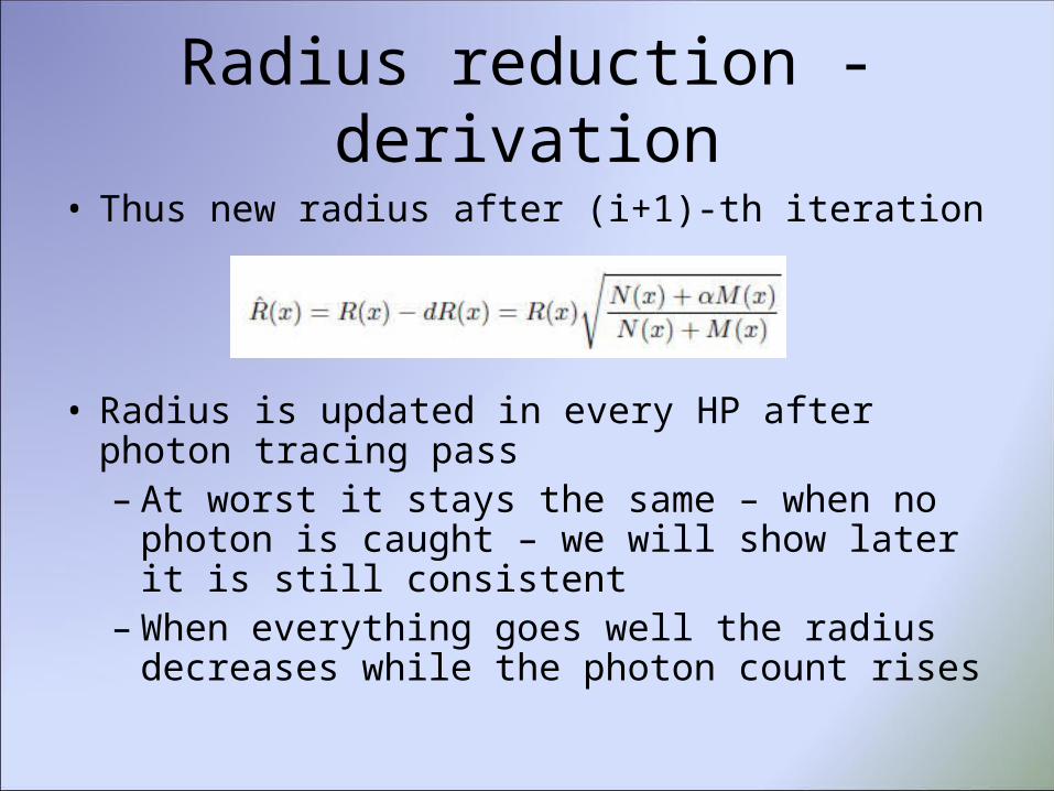
• Thus new radius after (i+1)-th iteration
• Radius is updated in every HP after photon tracing pass– At worst it stays the same – when no photon is
caught – we will show later it is still consistent– When everything goes well the radius decreases
while the photon count rises

Flux correction
• Cannot just average the illumination– We need to account for those lost photons disposed by α
• Unnormalized flux pre-multiplied by BRDF
© Hachisuka et al.

Flux correction
• We could keep the list of photons in every HP and subtract flux of those which fall out– Slow, memory demanding
• Better: assume both photon density and therefore the illumination are the same. Then
radiance doesn’t change• Results in:
Resulting radiance estimate
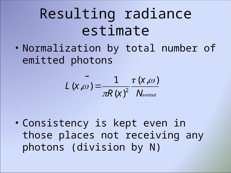
• Normalization by total number of emitted photons
• Consistency is kept even in those places not receiving any photons (division by N)
emittedN
x
xRxL
),(
)(
1),(
2
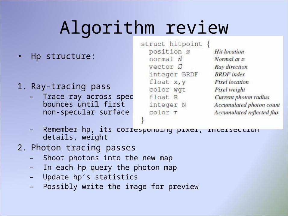
Algorithm review• Hp structure:
1. Ray-tracing pass– Trace ray across specular
bounces until first non-specular surface is hit
– Remember hp, its corresponding pixel, intersection details, weight2. Photon tracing passes
– Shoot photons into the new map– In each hp query the photon map– Update hp’s statistics– Possibly write the image for preview

Main disadvantages of PPM
• Biased– Still, consistent– In theory we can get arbitrarily precise solution (no
memory restrictions)
• Bad behaviour on glossy reflections– Could be solved by casting more samples => more hps =>
memory restrictions
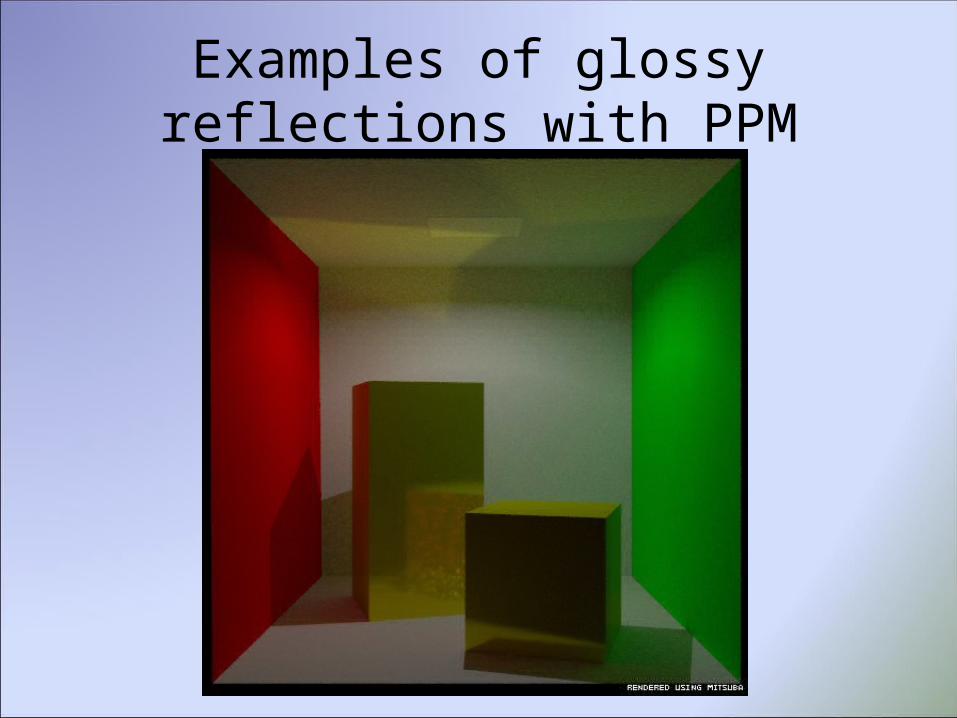
Examples of glossy reflections with PPM

Stochastic PPM
Jiří Vorba
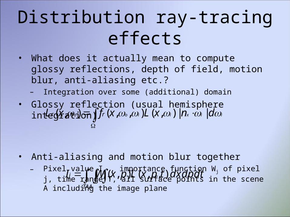
Distribution ray-tracing effects
• What does it actually mean to compute glossy reflections, depth of field, motion blur, anti-aliasing etc.?– Integration over some (additional) domain
• Glossy reflection (usual hemisphere integration)
• Anti-aliasing and motion blur together– Pixel value Ij , importance function Wj of pixel j, time range T, all
surface points in the scene A including the image plane
iixiioo dnxLxfxL rr ||),(),,(),(
dtdpdxtpxLpxWITAA
jj ),,(),(

How would have we done it by PPM?
• For brevity suppose that we want to know the average value of radiance over some region S (e.g. anti-aliasing) and we have n uniformly distributed samples xk over the region S
• This needs keeping the track of n HP’s statistics for all sets of HPs

How to overcome the memory boundary?
• We can keep the shared statistics for the region S– The region S in implementations is usually the pixel– Thus we are fine with one HP for every pixel
• For region S it is important to share the radius and α– It can vary between regions even at the beginning of the
algorithm if we want to– This is the only condition for consistency
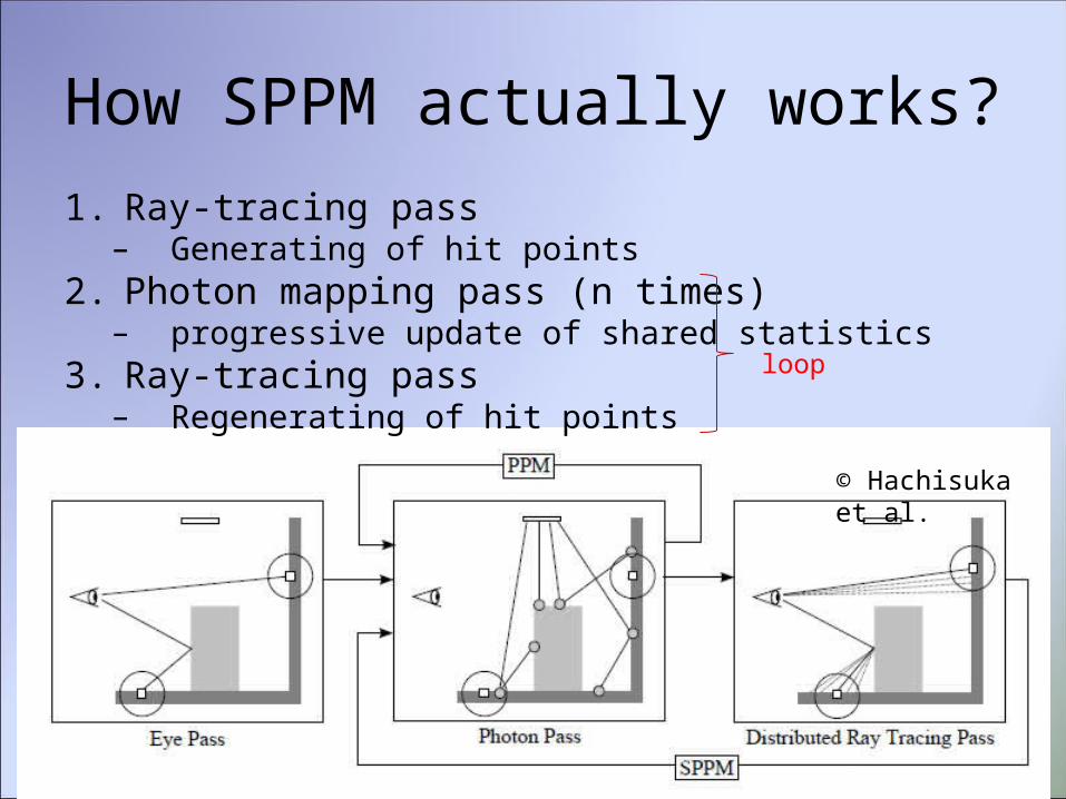
How SPPM actually works?1. Ray-tracing pass– Generating of hit points
2. Photon mapping pass (n times)– progressive update of shared statistics
3. Ray-tracing pass– Regenerating of hit points
loop
© Hachisuka et al.

PPM vs. SPPM
© Hachisuka et al.
Optimal light paths connection
Jiří Vorba
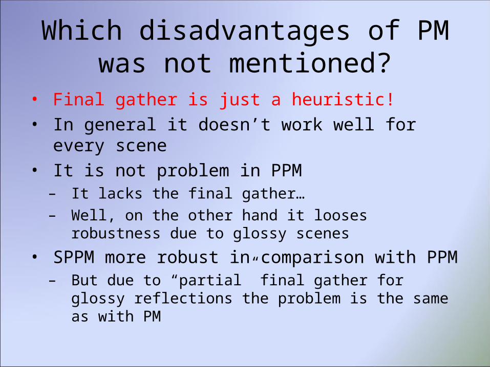
Which disadvantages of PM was not mentioned?
• Final gather is just a heuristic!• In general it doesn’t work well for every scene• It is not problem in PPM– It lacks the final gather…– Well, on the other hand it looses robustness due to
glossy scenes
• SPPM more robust in comparison with PPM– But due to “partial” final gather for glossy reflections
the problem is the same as with PM

Examples
© Jaroslav Křivánek
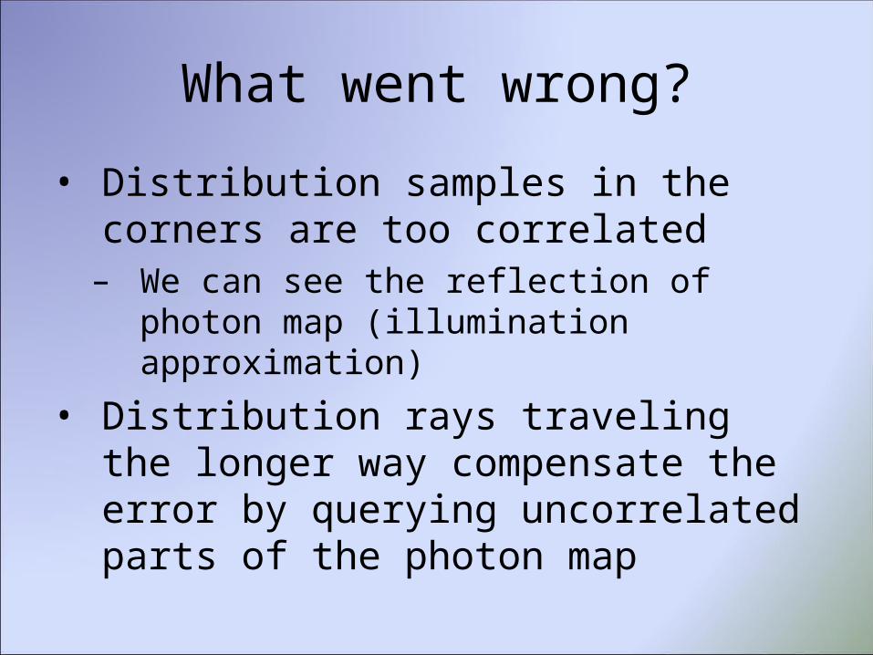
What went wrong?
• Distribution samples in the corners are too correlated– We can see the reflection of photon map
(illumination approximation)
• Distribution rays traveling the longer way compensate the error by querying uncorrelated parts of the photon map
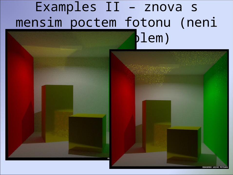
Examples II – znova s mensim poctem fotonu (neni videt problem)
What went wrong II
• Direct photon map visualization is good for caustic from highly glossy surface– It is not that good for overall appearance (direct
visualization of illumination approximation)• Indirect visualization (final gather) is good for
overall appearance– Turning the whole path into the ray-tracing is bad
for caustic • So question is: “When should we query the
photon map?”
What approach to try?• Inspiration by Erich Veach– Technique of Multiple Importance Sampling
• In bi-directional path-tracing he connects paths from light and from camera by weighting the whole path contribution– This prevents the same paths generated from different
sampling techniques to contribute twice to the overall illumination
• Radiance estimate (photon map query) is connection of paths as well– Could we somehow apply Veache’s approach?– It means more photon map queries on “the same final gather
path” and weight their contributions

Thank you
http://ms.mff.cuni.cz/~vorbj4am/pm_ppm_sppm.pptx