phenoncsu qtl ii: yandell © 20041 extending the phenotype model 1.limitations of parametric...

Pheno NCSU QTL II: Yandell © 2004 1

Extending the Phenotype Model1. limitations of parametric models 2-9

– diagnostic tools for QTL analysis– QTL mapping with other parametric "families"– quick fixes via data transformations

2. semi-parametric approaches 10-243. non-parametric approaches 25-31• bottom line for normal phenotype model

– may work well to pick up loci– may be poor at estimating effects if data not normal


1. limitations of parametric models• measurements not normal

– categorical traits: counts (e.g. number of tumors)• use methods specific for counts• binomial, Poisson, negative binomial

– traits measured over time and/or space• survival time (e.g. days to flowering)• developmental process; signal transduction between cells• TP Speed (pers. comm.); Ma, Casella, Wu (2002)

• false positives due to miss-specified model– how to check model assumptions?

• want more robust estimates of effects– parametric: only center (mean), spread (SD)– shape of distribution may be important


what if data are far away from ideal?

8 9 10 11 12 13 14 15 16

qqQq

QQ

no QTL?

8 9 10 11 12 13 14 15 16

qqQq

QQ

skewed?

8 9 10 11 12 13 14 15 16 17 18 19 20 21

qq

Qq

QQ

dominance?

0 1 2 3 4 5 6 7 8 9

qq

QqQQ

zeros?


diagnostic tools for QTL(Hackett 1997)

• illustrated with BC, adapt regression diagnostics• normality & equal variance (fig. 1)

– plot fitted values vs. residuals--football shaped?– normal scores plot of residuals--straight line?

• number of QTL: likelihood profile (fig. 2)– flat shoulders near LOD peak: evidence for 1 vs. 2 QTL

• genetic effects– effect estimate near QTL should be (1–2r)a– plot effect vs. location


marker density & sample size: 2 QTLmodest sample size

dense vs. sparse markerslarge sample size

dense vs. sparse markers

Wright Kong (1997 Genetics)


robust locus estimate for non-normal phenotype

Wright Kong (1997 Genetics)

large sample size &dense marker map:no need for normality

but what happens formodest sample sizes?


useful models & transformations• binary trait (yes/no, hi/lo, …)

– map directly as another marker– categorical: break into binary traits?– mixed binary/continuous: condition on Y > 0?

• known model for biological mechanism– counts Poisson – fractions binomial– clustered negative binomial

• transform to stabilize variance– counts Y = sqrt(Y)– concentration log(Y) or log(Y+c) – fractions arcsin(Y)

• transform to symmetry (approx. normal)– fraction log(Y/(1-Y)) or log((Y+c)/(1+c-Y))

• empirical transform based on histogram– watch out: hard to do well even without mixture– probably better to map untransformed, then examine residuals


2. semi-parametric QTL• phenotype model pr(Y|Q,) = f(Y)exp(YQ)

– unknown parameters = (f, )• f (Y) is a (unknown) density if there is no QTL = (qq, Qq, QQ)• exp(YQ) `tilts’ f based on genotype Q and phenotype Y

• test for QTL at locus Q = 0 for all Q, or pr(Y|Q,) = f(Y)

• includes many standard phenotype modelsnormal pr(Y|Q,) = N(GQ,2)

Poisson pr(Y|Q,) = Poisson(GQ)exponential, binomial, …, but not negative binomial


QTL for binomial data• approximate methods: marker regression

– Zeng (1993,1994); Visscher et al. (1996); McIntyre et al. (2001)

• interval mapping, CIM– Xu Atchley (1996); Yi Xu (2000)– Y ~ binomial(1, ), depends on genotype Q– pr(Y|Q) = (Q)Y (1 – Q)(1–Y)

– substitute this phenotype model in EM iteration

• or just map it as another marker!– but may have complex


EM algorithm for binomial QTL

• E-step: posterior probability of genotype Q

• M-step: MLE of binomial probability Q

),,,|(pr sum

),,,|(pr sum

numerator of sum

)1())(,|(pr),,,|(pr

)1(

Qiii

QiiiiQ

Q

YQ

YQi

Qii

XYQ

XYQY

XQXYQ

ii


threshold or latent variable idea• "real", unobserved phenotype Z is continuous• observed phenotype Y is ordinal value

– no/yes; poor/fair/good/excellent– pr(Y = j) = pr(j–1 < Z j)– pr(Y j) = pr(Z j)

• use logistic regression idea (Hackett Weller 1995)– substitute new phenotype model in to EM algorithm– or use Bayesian posterior approach– extended to multiple QTL (papers in press)

1)]exp(1[)|(pr)|(pr jQj GQZQjY


quantitative & qualitative traits• Broman (2003): spike in phenotype

– large fraction of phenotype has one value– map binary trait (is/is not that value)– map continuous trait given not that value

• multiple traits– Williams et al. (1999)

• multiple binary & normal traits• variance component analysis

– Corander Sillanpaa (2002)• multiple discrete & continuous traits• latent (unobserved) variables


other parametric approaches• Poisson counts

– Mackay Fry (1996)• trait = bristle number

– Shepel et al (1998)• trait = tumor count

• negative binomial– Lan et al. (2001)

• number of tumors

• exponential– Jansen (1992)

Mackay Fry (1996 Genetics)


semi-parametric empirical likelihood• phenotype model pr(Y|Q,) = f(Y) exp(YQ)

– “point mass” at each measured phenotype Yi

– subject to distribution constraints for each Q:

1 = sumi f(Yi) exp(YiQ)

• non-parametric empirical likelihood (Owen 1988)L(,|Y,X) = producti [sumQ pr(Q|Xi,) f(Yi) exp(YiQ)]

= producti f(Yi) [sumQ pr(Q|Xi,) exp(YiQ)]

= producti f(Yi) wi

– weights wi = w(Yi|Xi,,) rely only on flanking markers• 4 possible values for BC, 9 for F2, etc.

• profile likelihood: L(|Y,X) = max L(,|Y,X)


semi-parametric formal tests• partial empirical LOD

– Zou, Fine, Yandell (2002 Biometrika)

• conditional empirical LOD– Zou, Fine (2003 Biometrika); Jin, Fine, Yandell (2004)

• has same formal behavior as parametric LOD– single locus test: approximately 2 with 1 d.f.– genome-wide scan: can use same critical values– permutation test: possible with some work

• can estimate cumulative distributions– nice properties (converge to Gaussian processes)


partial empirical likelihoodlog(L(,|Y,X)) = sumi log(f(Yi)) +log(wi)

now profile with respect to ,log(L(,|Y,X)) = sumi log(fi) +log(wi)

+ sumQ Q(1-sumi fi exp(YiQ))

partial likelihood: set Lagrange multipliers Q to 0force f to be a distribution that sums to 1

point mass density estimates ),|(pr)exp(sum with sum -1 iQiQiiii XQYwwf


histograms and CDFs

histogram

Den

sity

6 8 10 12 14

0.00

0.10

0.20

Y = phenotype

fre

qu

en

cy

6 8 10 12 140.

00.

40.

8

+ +++++++++++++++++++

++++++++++++++++

++++++++++++++++

++++++++++++++++++++++++

++++++++++++++++

+++++++ +

Y = phenotypecu

mu

lativ

e fr

eq

ue

ncy

cumulative distribution

histograms capture shapebut are not very accurate

CDFs are more accuratebut not always intuitive


rat study of breast cancerLan et al. (2001 Genetics)

• rat backcross– two inbred strains

• Wistar-Furth susceptible

• Wistar-Kyoto resistant

– backcross to WF

– 383 females

– chromosome 5, 58 markers

• search for resistance genes

• Y = # mammary carcinomas

• where is the QTL? dash = normalsolid = semi-parametric


what shape histograms by genotype?WF/WF WKy/WF

line = normal, + = semi-parametric, o = confidence interval


conditional empirical LOD• partial empirical LOD has problems

– tests for F2 depends on unknown weights

– difficult to generalize to multiple QTL

• conditional empirical likelihood unbiased– examine genotypes given phenotypes

– does not depend on f(Y)

– pr(Xi) depends only on mating design

– unbiased for selective genotyping (Jin et al. 2004)

pr(Xi|Yi,,,Q) = exp(YiQ) pr(Q|Xi|) pr(Xi) / constant


spike data exampleBoyartchuk et al. (2001); Broman (2003)133 markers, 20 chromosomes116 female miceListeria monocytogenes infection


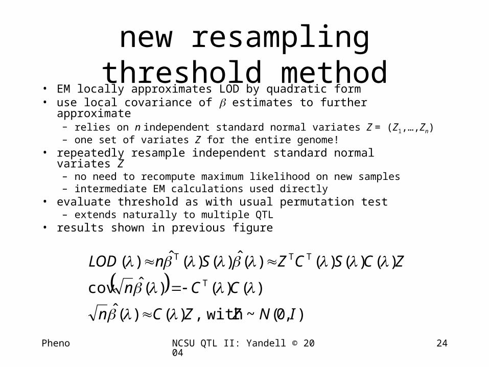
new resampling threshold method

• EM locally approximates LOD by quadratic form• use local covariance of estimates to further approximate

– relies on n independent standard normal variates Z = (Z1,…,Zn)– one set of variates Z for the entire genome!

• repeatedly resample independent standard normal variates Z– no need to recompute maximum likelihood on new samples– intermediate EM calculations used directly

• evaluate threshold as with usual permutation test– extends naturally to multiple QTL

• results shown in previous figure

),0(~ with ,)()(ˆ

)()()(ˆcov

)()()()(ˆ)()(ˆ)(T

TTT

INZZCn

CCn

ZCSCZSnLOD


3. non-parametric methods• phenotype model pr(Y|Q, ) = FQ(Y)

= F = (Fqq,FQq,FQQ) arbitrary distribution functions

• interval mapping Wilcoxon rank-sum test– replaced Y by rank(Y)

• (Kruglyak Lander 1995; Poole Drinkwater 1996; Broman 2003)

– claimed no estimator of QTL effects

• non-parametric shift estimator– semi-parametric shift (Hodges-Lehmann)

• Zou (2001) thesis, Zou, Yandell, Fine (2002 in review)

– non-parametric cumulative distribution• Fine, Zou, Yandell (2001 in review)

• stochastic ordering (Hoff et al. 2002)


rank-sum QTL methods• phenotype model pr(Y|Q, ) = FQ(Y) • replace Y by rank(Y) and perform IM

– extension of Wilcoxon rank-sum test– fully non-parametric (Kruglyak Lander 1995; Poole Drinkwater 1996)

• Hodges-Lehmann estimator of shift – most efficient if pr(Y|Q, ) = F(Y+Q)– find that matches medians

• problem: genotypes Q unknown• resolution: Haley-Knott (1992) regression scan

– works well in practice, but theory is elusive• Zou, Yandell Fine (Genetics, in review)


non-parametric QTL CDFs• estimate non-parametric phenotype model

– cumulative distributions FQ(y) = pr(Y y |Q)

– can use to check parametric model validity

• basic idea:

pr(Y y |X,) = sumQ pr(Q|X,)FQ(y)

– depends on X only through flanking markers– few possible flanking marker genotypes

• 4 for BC, 9 for F2, etc.


finding non-parametric QTL CDFs

• cumulative distribution FQ(y) = pr(Y y |Q)

• F = {FQ, all possible QT genotypes Q}

– BC with 1 QTL: F = {FQQ, FQq}

• find F to minimize over all phenotypes ysumi [I(Yi y) – sumQ pr(Q|X,)FQ(y)]2

• looks complicated, but simple to implement


non-parametric CDF properties

• readily extended to censored data– time to flowering for non-vernalized plants– Fine, Zou, Yandell (2004 Biometrics J)

• nice large sample properties– estimates of F(y) = {FQ(y)} jointly normal– point-wise, experiment-wise confidence bands

• more robust to heavy tails and outliers• can use to assess parametric assumptions


what QTL influence flowering time? no vernalization: censored survival

• Brassica napus– Major female

• needs vernalization

– Stellar male• insensitive

– 99 double haploids

• Y = log(days to flower)– over 50% Major at QTL

never flowered

– log not fully effective grey = normal, red = non-parametric


what shape is flowering distribution?B. napus Stellar B. napus Major

line = normal, + = non-parametric, o = confidence interval

phenoncsu qtl ii: yandell © 20041 extending the phenotype model 1.limitations of parametric...

Documents

number of qtl

qtl presentmixture

geneticsncsu qtl

fqyncsu qtl

locationncsu qtl

normalncsu qtl

importantncsu qtl

residualsncsu qtl