Phenomenology of a Two-Higgs-Doublet Model for Neutrino

Mass

by

Shainen Davidson

A thesis submitted to the

Faculty of Graduate and Postdoctoral Affairs

in partial fulfillment of the requirements

for the degree of

Master of Science

Department of Physics

Carleton University

Ottawa-Carleton Institute of Physics

Ottawa, Canada

September 8, 2010

Copyright © 2010 Shainen Davidson

1*1 Library and Archives Canada

Published Heritage Branch

395 Wellington Street OttawaONK1A0N4 Canada

BibliothSque et Archives Canada

Direction du Patrimoine de l'6dition

395, rue Wellington OttawaONK1A0N4 Canada

Your file Votre reference ISBN: 978-0-494-71577-2 Our file Notre reference ISBN: 978-0-494-71577-2

NOTICE:

The author has granted a non­exclusive license allowing Library and Archives Canada to reproduce, publish, archive, preserve, conserve, communicate to the public by telecommunication or on the Internet, loan, distribute and sell theses worldwide, for commercial or non­commercial purposes, in microform, paper, electronic and/or any other formats.

The author retains copyright ownership and moral rights in this thesis. Neither the thesis nor substantial extracts from it may be printed or otherwise reproduced without the author's permission.

AVIS:

L'auteur a accorde une licence non exclusive permettant a la Bibliotheque et Archives Canada de reproduire, publier, archiver, sauvegarder, conserver, transmettre au public par telecommunication ou par rinternet, preter, distribuer et vendre des theses partout dans le monde, a des fins commerciales ou autres, sur support microforme, papier, electronique et/ou autres formats.

L'auteur conserve la propriete du droit d'auteur et des droits moraux qui protege cette these. Ni la these ni des extraits substantiels de celle-ci ne doivent etre imprimes ou autrement reproduits sans son autorisation.

In compliance with the Canadian Privacy Act some supporting forms may have been removed from this thesis.

While these forms may be included in the document page count, their removal does not represent any loss of content from the thesis.

Conformement a la loi canadienne sur la protection de la vie privee, quelques formulaires secondaires ont ete enleves de cette these.

Bien que ces formulaires aient inclus dans la pagination, il n'y aura aucun contenu manquant.

•+•

Canada

Abstract The Standard Model includes massless chiral left-handed neutrinos; however,

experiment suggests that the neutrino is a massive particle. We present an exten­

sion to the Standard Model that gives neutrinos a tiny mass through a second Higgs

doublet with small vacuum expectation value, while forbidding Majorana neutrino

masses. A Monte Carlo simulation of the signal process pp —» H+H~ —> ££'u£U£t and

relevant background for CERN's Large Hadron Collider was conducted. It was con­

cluded that 5<r discovery statistics could be gathered for the model with a minimum

of 6 (184) fb"1 of data at 14 TeV beam energy for MH+ = 100 (300) GeV.

li

To Annie, for everything; and to my mother, in case she sees this.

hi

Acknowledgements I would like to thank my advisor, Heather Logan, without whose support

this would not have been possible. Heather has taught me more about the natural

world than I would have thought could fit in my head. Working with her has been a

formative experience in every positive way.

I have also benefitted greatly from the learning environment provided by the

faculty in the Carleton University Department of Physics. I would like to thank the

Department for providing financial aid during my studies.

This work was supported by the Natural Sciences and Engineering Research

Council of Canada.

IV

Statement of Originality Chapter 2 (Background) is a review of known results taken from the literature.

The particle physics model described in Chapter 3 was built by my advisor,

Heather Logan. I calculated the masses in the last year of my BSc and the branching

ratios in the summer before the beginning of my MSc during an NSERC USRA

summer research term.

The phenomenology of Chapter 4 is my own work, in consultation with Heather

Logan. I worked on the following during the USRA summer research term prior to

beginning my MSc: big-bang nucleosynthesis (BBN) of Sec. 4.1; tree-level muon and

tau decays of Sec. 4.2; the parton-level cross section calculation of Eq. 4.6; and

the numerical cross section results from PROSPINO for LHC at both tree level and

next-to-leading order of Sec. 4.5.

The LEP mass limits of Sec. 4.3 and the L —• ^7 calculation of Sec. 4.4 and

Appendix A were begun after I started my MSc.

The model, together with the limits from BBN and LEP, the results from

L —» £j and tree-level muon and tau decay, and the cross sections for charged Higgs

pair production at the LHC have been published in Ref. [1].

The LHC phenomenology study in Chapter 5 is my own work, in consultation

with Heather Logan, and was begun and completed after I began my MSc. A draft

journal article with this work is in preparation [2].

v

Contents

1 Introduction 1

2 Background 3

2.1 Content of a field theory 3

2.2 Dirac and Majorana neutrinos 6

2.3 Neutrinos 13

2.3.1 Fundamental particles and forces 13

2.3.2 Neutrino Mass and Oscillations 13

2.3.3 Neutrino hierarchies 19

2.3.4 Mechanisms of neutrino mass 20

3 Model 21

3.1 Introduction 21

3.2 Field Content 22

3.3 Symmetry breaking 23

vi

3.4 Mass eigenstates 29

3.5 Decays 31

4 Phenomenology 34

4.1 Big bang nucleosynthesis 34

4.2 Tree-level muon and tau decay 38

4.3 LEP-II constraints on H+ mass 42

4.4 Decay rate of L -> ^7 43

4.5 Charged Higgs pair production at LHC 47

4.5.1 Parton distribution functions 48

4.5.2 Comparison to triplet model 49

5 LHC signal/background study 52

5.1 Introduction 52

5.2 Monte Carlo simulations 53

5.3 MadGraph/MadEvent 54

5.4 PYTHIA-PGS 56

5.5 Signal and Background Processes 57

5.6 QCD Corrections 59

5.7 Selection Cuts 62

5.8 Discussion 67

vn

6 Conclusion 70

A Calculation of L -» £j 72

References 83

viii

List of Tables

2.1 The neutrino parameter values used in this paper, with 2a uncertain­

ties. From Ref. [13] 18

5.1 The cuts applied to the simulated data to get the cleanest signal. . . 62

5.2 Cut efficiency for pp —> e+e~p™lss via H+H~. The efficiency of each

cut is calculated as the number of events that passed the cut divided

by the number of events that passed the previous cut. The cumulative

efficiency is the number of events that pass all the cuts divided by the

original number of events. Recall, H'T > 200 GeV for MH+ = 100 GeV,

and H'T > 600 GeV for MH+ = 300 GeV 64

5.3 As in Table 5.2 but for background for pp —» e+e~p™lss 64

5.4 As in Table 5.2 but for pp -> /X+/J~PTW8 v i a H+H~ 65

5.5 As in Table 5.2 but for background for pp —> ^+/i~p™ss. (*To be

conservative, in the luminosity plots Figs. 5.2 and 5.3 this cut efficiency

was set to 0.00002, which is the efficiency from the e+e"p^l8S final state

simulation. This has a negligible effect on luminosity required for 5a.) 65

5.6 As in Table 5.2 but for pp - • e±^p™ss via H+H~ 66

IX

5.7 As in Table 5.2 but for background for pp —> e±/jJTp™lss. (*To be

conservative, in the luminosity plots Figs. 5.2 and 5.3 this cut efficiency

was set to 0.00002, which is the efficiency from the e+e~p™lss final state

simulation. This has a negligible effect on luminosity required for 5a.) 66

A.l Feynman rules used in the L —> £j calculation. For the QED scalar

vertex, p (jfi) momentum of the incoming (outgoing) H~ 73

x

List of Figures

2.1 The two possible hierarchies for neutrino masses (inspired by image

from Lawrence Berkeley National Lab website [14]) 19

3.1 A 2-dimensional representation of spontaneous symmetry breaking. . 25

3.2 A 2-dimensional representation of explicit symmetry breaking 28

3.3 Charged Higgs decay branching fractions to ez/, fiu, and rv as a func­

tion of the lightest neutrino mass 33

4.1 Values for the charged current coupling constants (showing the two

sigma experimemtal limits) versus v2, with the mass of the charged

Higgs set at 100 GeV (a larger charged Higgs mass will result in a

lower constraint) and normal hierarchy neutrinos with a smallest mass

of (a) and (b) 0 eV, and (c) and (d) 1 eV 40

4.2 Same as Figure 4.1 but with inverted hierarchy neutrinos 41

4.3 Limit on mass of charged Higgs for various values of the lightest neu­

trino mass for (a) normal hierarchy and (b) inverted hierarchy 44

4.4 The three possible first-order Feynman diagrams for /i —> e 7 via

charged Higgs 45

4.5 Branching ratios for L —• ^7 plotted against neutrino parameters with

large effects, for MH+ = 100 GeV and v2 — 3 eV. In all cases the

normal hierarchy is used, as the inverted hierarchy plots are similar.

In (a) the expected limit from the MEG experiment after running to

the end of 2011 [30] is plotted, and it is apparent that for certain values

of neutrino parameter space the effects of the model would be noticed. 47

4.6 LO and NLO production cross-section at LHC (14 TeV) for charged

Higgs pair 51

5.1 The tree-level Feynman diagrams for the process uu —> HJrH~ —>

e~veii+vll, produced by MadGraph 55

5.2 Luminosity required for a 5a discovery if MH+ = 100 GeV for (a) nor­

mal hierarchy (NH) and (b) inverted hierarchy (IH) neutrino masses.

The spread in the luminosity values is due to scanning over the 2a range

on the parameters of the neutrino mixing matrix and mass differences. 68

5.3 As in Fig. 5.2 but for MH+ = 300 GeV 68

xn

Chapter 1

Introduction

The Standard Model (SM) includes massless chiral left-handed neutrinos; however,

experiment suggests that the neutrino is a massive particle. It is possible to minimally

extend the SM to give neutrino masses by introducing right-handed neutrinos and

extending the Higgs sector to couple to both types of neutrinos as it does to the

other fermions. However, this introduces two problems. First, since the neutrinos

are much lighter than any other known massive particle, we have to introduce nine

exceptionally tiny Yukawa couplings y\ by hand. It would be preferable to have a

reason for the tiny masses. Second, since right-handed neutrinos are not charged

under the electroweak or strong interactions, gauge invariance does not forbid them

from having a Majorana mass. A neutrino Majorana mass would make them their

own antiparticles, a phenomenon that has yet to appear in experimental results.

With these two issues in mind, we present an extension to the Standard Model

that gives neutrinos a tiny mass through a second Higgs doublet with small vacuum

expectation value, while forbidding Majorana neutrino masses. It is presented in full

in Chapter 3.

1

We then examine the phenomenology of the model (Chapter 4), including the

constraints imposed by the early universe and experiment. We also compare the cross

section of the most detectable production process, charged Higgs production, to that

of a triplet model with similar phenomenology.

Finally, we examine how the model can be detected experimentally. Chap­

ter 5 illustrates how Monte Carlo techniques were employed to test the feasibil­

ity of discovering this model at CERN's Large Hadron Collider (LHC). The signal

pp —> H+H~ —» ££'p™lss with ££' = e+e~, /i+/x" or e±/x=F was simulated along with

background from di-boson and top-pair production. For MH+ = 100 (300) GeV, we

find 5a discovery statistics with a minimum of 6 (184) fb -1 of data at 14 TeV beam

energy.

We begin by giving some background on neutrino masses in Chapter 2.

2

Chapter 2

Background

2.1 Content of a field theory

We represent particles as mathematical objects called fields. We present the content of

a particular quantum field theory model of particle physics by presenting the quantum

fields and the form of the Lagrangian density, dictated by the symmetries the model

imposes on the fields.

Much of the following discussion is based on Ref. [3].

Since we wish physics to work the same regardless of frame of reference, we

design the Lagrangian to be Lorentz invariant. Various ways of changing frames

of reference (speeding up by 0.9c, rotating by 43° in some plane) can be taken to

be members of a group, the Lorentz group of type SO(3,1), with generators J% for

rotation and K% for boosts, that satisfy the following algebra:

[Jl? J3] = iCijkJk (2.1)

3

[Kt, Kj] =-ieljkJk (2.2)

[Jt,K]]=ietjkK3, (2.3)

where i, j , k run from 1 to 3 and eljk is the totally antisymmetric tensor with eu3 = +1-

We can disentangle the algebra by defining new generators

A = \(Jt + iKt) (2.4)

Bx = ^{Jt-iKx\ (2.5)

that satisfy the algebra

[A,, Aj] = ieljkAk (2.6)

[BuBj] = ieljkBk (2.7)

[A,B3] = 0, (2.8)

which are the algebras of the group SU{2) x SU(2). There are various representations

of this algebra, corresponding to matrices of various sizes; these are labeled in the

usual way by integer and half-integer "spins", where spin s corresponds to a square

matrix of length 2s + 1. We label the spins of the two series of generators as (a, b).

The simplest case is when both generators are given spin 0, so (0, 0), thus

A = Bt = 0, (2.9)

which leads to rotation and boost generators of

Jt = Kt = 0, (2.10)

4

thus the identity group. The fields that correspond to this representation are the

scalar fields, which transform under rotations and boosts as

<£-<£. (2.11)

To construct a Lorentz invariant Lagrangian, we can insert terms with as many factors

of (ft as we want; however, terms of (f)n with n > 2 cannot be solved analytically, so

to a first order approximation, I will only put in (f)2. I can also place derivatives of

(f) in the Lagrangian; the only one that is both Lorentz invariant and can be solved

exactly is (<90)2. Thus the Lorentz invariant solvable Lagrangian is

C = a(d(j))2 -b(f>2. (2.12)

We can apply the Euler-Lagrange equation, <9M ( a££ ,x J — | ^ = 0, to get

2ad2(f) + 2b(j) = 0. (2.13)

We can write the field in momentum space using a Fourier transform as

so the derivative simply pulls out (—ip)2 — —p2 = — (E2 — p1), so we get

2{aE2 - af - b)(f) = 0. (2.15)

Since mass is defined to satisfy the relationship E2 — p2 — m2 — 0, b/a — m2. We

can multiply the Lagrangian by an overall factor without changing the physics, so it

5

is conventional to write Eq. 2.12 as

£=^)2-lmV. (2-16)

Thus, for a scalar field, the term in the Lagrangian with two fields tells us the value

of m2. Fermions, however, are objects that transform under Lorentz transformations

differently, and that case will be examined in the next section.

2.2 Dirac and Majorana neutrinos

The next simplest representation of the SU{2) x 517(2) Lorentz symmetry is ( | ,0),

which corresponds to generators of

A = \<?r (2-17)

Bx = 0 (2.18)

which gives Lorentz rotation and boost generators

J% = ±<T, (2.19)

Kx = - % - o % . (2.20)

The <7j are 2 x 2 matrices, so clearly the fields they act on are two-component vectors,

called Weyl spinors, and transform when rotated or boosted as

X - e-Wx (2-21)

6

X - + e ^vx, (2.22)

where the vector 6t defines some 3-dimensional rotation angle, and rjx is the rapidity,

defined by v = tanhr?, where v is the velocity in units of the speed of light.

If I want to make mass terms out of these spinors, I need to find a way to

combine two of them in a term with no other vectors such that the term is Lorentz

invariant. Let's try

(2.23) £ = 2m(xT eX + h-c)>

in which e the antisymmetric matrix {eX] = —eJX) with e2 = I and h.c. stands for the

hermitian conjugate.* Write the Lorentz transformation as a matrix M, such that

T-K/rT, X1 eX -> X M1 eMX- (2.24)

Looking at the middle section, we have

MZpepyMrf = efrM0aMl5

= e12(MlaM2S - M2aMu) (

ei2

V

0 MnM22 - M2lMl2

M12M21 - M22Mn 0 aS

\

0 e12(MnM22 - M2lMx2)

-e12(MnM22 - M21M12) 0

(2.25)

(2.26)

(2.27)

(2.28) Q.8

= eas detM (2.29)

(2.30)

*So that xTeX is n°t equal to zero, we define the components of \ to be Grassmann numbers, which are defined to satisfy {xi, X2} = X1X2 + X2X1 = 0.

7

where in the last step, we use detM = 1 for SU(N) matrices.

It turns out that there is one more operation relating to symmetries we want

to consider in our physics. The change of coordinates x —• — x and p —> — p is known

as parity. We can accomplish this transition in terms of the Lorentz generators as

J% —> Jx and K% —> — K%\ this is equivalent to changing representations (|, 0) —> (0, | )

[4]. We can make a four-component spinor out of the Weyl spinor that transforms

under Lorentz transformations using both representations as

f X (

0 X

J y e X J

(2.31)

/ \ X I

[ex* )

e-\n-e o \ I \ X

\ 0 e\ve I \eX- J

(2.32)

A 4-spinor that transforms under Lorentz transformations in this way that is made

up of only one Weyl spinor is called a Majorana spinor, and is labeled as ipM-

We can write the Lorentz invariant mass term we discovered before as

£ = —^rntpM'4'M, (2.33)

where ip = V 7°> a n d 7° = 0 /

/ 0 (this form is required for Lorentz invariance).

/ We can also make a Lorentz invariant kinetic term, i.e., a term with derivatives, with

CK = iipMl^^M, (2.34)

where the four 7^ are the four gamma matrices defined by {7/*,7I/} = 1rfv. The

8

explicit form I gave for 70 constrains the form of the other gamma matrices; this is

called the Weyl basis. We thus construct a solvable Lagrangian

£ = $M(i>l^-^rri)iPM. (2.35)

We apply the Euler-Lagrange equation to get the equation of motion for this field.

Applying d^ f d^C *\) — J^r = 0 gives us the traditional form of the equation,

( 2 7 ^ - m)^M = 0. (2.36)

To see what this tells us about the mysterious parameter m, we multiply both sides

by [i^vdv + m) to get — {^(ydv^^d^ + m2)ipM — 0. Since derivatives commute, we can

write 7i,<9^7Ai9/i as \{^iv^y}dud^ — d^d^ by the definition of the gamma matrices.

We thus end up with the relation

(d^ + m2)^M = 0, (2.37)

from which, by doing the same conversion to momentum space we did in Eq. 2.13,

we get the mass energy relation, proving that m really is the mass.

If we want these spinors to represent the charged leptons in the SM, we run

into a problem. Since they carry electric charge, they obey an additional symmetry,

the SU(2) x U(l) electro-weak symmetry. If we try to perform an internal SU{2)

symmetry transformation on a set of Weyl spinors in the mass term we derived be­

fore (representing the internal symmetry with matrix U and roman indices, and the

9

Lorentz indices with greek letters, repeated indices summed), we get

Xl^pXl - UabX

baeaPUacx% (2.38)

which is only invariant if UTU = 1, not the case for SU(2). The obvious thing to

try is to add another antisymmetric matrix for this new SU{2) symmetry, which will

preserve the symmetry just as it did for the Lorentz 5t/(2); however, if we try that

we get

-ab-.a.b _ _a6 . . 6 . . a - _a6_ . 6 . .a _ s-ba„b. .a _ ^ab-,a-,b / o QQN e a / ^ XaX/3 ~ " ^ a / ^ X / ? X a = e / ?a£ X/?Xa ~ " ^ a 6 X/?Xa ~ ~ e a / ^ X a X / 3 , 1 ^ 9 )

where in the second step I used the fact that the x are Grassmann numbers, that is

{xSoX/3} — 0; in the third and fourth step the anti-symmetry of e; and in the last

step I simply relabeled the dummy indices. Since this term is equal to its negation,

clearly the term must vanish. Thus we cannot construct Majorana mass terms for

sets of Weyl spinors that obey an internal SU(2) symmetry.'1'

To create some kind of mass term that will obey the SU{2) symmetry, we

note that such transformations are of the form WU = 1. We saw previously that if

we have two Weyl spinors that transform the same way, we get UTU, so to get the

desired result, we create a new spinor that transforms as the complex conjugate of

the first spinor:

X-+UX (2.40)

f -> U% (2.41)

^Note that the U(l) symmetry will also forbid this term. Under a U(l), x ~> e~iq6X, a n d so XTeX —* e~2iq6XTeXi clearly not invariant. We will use this to forbid Majorana masses in our model, discussed in Chapter 3.

10

We can then construct a Lorentz invariant and internal SU{2) invariant term that

looks like

C = m(fex + h.c). (2.42)

We can again make a four-component spinor that transforms under parity as

/

< / , =

V

X (2.43)

called a Dirac spinor, which we can use to construct a term that decomposes into Eq.

2.42,

C = -m^V- (2-44)

We thus construct a Lagrangian in the same form as Eq. 2.35, but with Dirac spinors:

C = ^{il^ - m)^, (2.45)

to which we can apply the Euler-Lagrange equation to get the famous Dirac equation,

( 2 7 ^ - m)ip = 0, (2.46)

which allows us to determine that m is indeed the mass.

We often talk about left-handed and right-handed fermions, which are math­

ematically defined as

/ 1 - 7 s , WL = —z—W =

V 0 / (2.47)

11

/ i + 75 , ' o ^ (2.48)

where 75 = Z7°717273, which in the Weyl basis is 75 = ' - / o ^

V 0 / 7 We can further construct something called the conjugate spinor that flips the

field content of the spinor:

r 0*1,* cyty:

—e 0

0 e 7 \J u7

0 /

/ 0

ex* 7

(2.49)

(2.50)

(2.51)

The purpose of defining this is that generally one writes Lagrangians in terms of

Dirac spinors, often with the left- and right-handed components projected out. For

example, the Dirac masses for the neutrinos will be displayed later in this paper as

CD = -m(ipLil;R + h.c.). (2.52)

Using the conjugate spinor notation, we can also write Majorana mass terms in terms

of Dirac spinors as

(2.53) CM = -om((V'c)flV'i, + h-c).

12

2.3 Neutr inos

2.3.1 Fundamental particles and forces

The fundamental particles described by the Standard Model (SM) are the quarks,

leptons, force carrier bosons, and the Higgs particle; all these particles have been

experimentally verified, except for the Higgs boson. The three forces mediated by

the force carriers are the electro-magnetic force, mediated by the photon (written as

7); the weak force, mediated by the W± and Z bosons; and the strong nuclear force,

mediated by the eight gluons g. Gravity is not accounted for in the SM.

The six leptons charged under the electro-magnetic force are the e~, /i~, and

r~, and their antiparticles with positive electric charge. There are an additional six

leptons with no electric charge, the neutrinos (written as v% and v% for the antiparticle).

The neutrinos were originally distinguished from each other according to which type

of charged lepton they would interact with. As the only force they feel is the weak

force, the only interaction possible is either with a Z boson or a W±. In the case

of the interaction with a W±, the 3-point interaction includes a charged lepton. For

example, when a \i~ decays, it uses the weak force to decay as pT —• e~Pez/M: the yT

turns into a v^ by emitting a virtual W~, and then the W~ decays into an e~ and its

companion antineutrino, the ve. Thus one can identify the neutrinos by their weak

eigenstates, labeled ve, v^, vT, and their antiparticles.

2.3.2 Neutrino Mass and Oscillations

Originally it was thought that the neutrinos were massless, and thus the only differ­

ence between the neutrinos would be the charged lepton with which they interact.

13

However, it has been discovered that neutrinos do have mass, although they are very

light (at this point the mass is known to be less than 2 eV from beta decay exper­

iments [5]). The evidence for neutrino mass came originally from the detection of

neutrinos coming from the sun: less ve were detected than postulated by theory [6].

Giving neutrinos mass solves this discrepancy in the following way. When

particles with mass propagate through space they act as plane waves which oscillate

according to their energy, which can be written as

\v%) = e~ip'x = e~l{Et-fx) = e~im^\ (2.54)

where r is the time in the neutrino's rest frame. If the mass eigenstates and weak

flavour eigenstates are not the same, then a particular weak flavour eigensate can be

written as 3

where the vg are the weak flavour eigenstates, the v% are the mass eigenstates, and U^

is a unitary matrix that describes the mixing between the weak and mass eigenstates

of the neutrinos, known as the Pontecorvo-Maki-Nakagawa-Sakata (PMNS) matrix

[7]-

Then, if the masses of the neutrinos are different, there is an amplitude for a

neutrino to be created in one weak flavour eigenstate and end up as a different one:

3

AmpK - ut2) = £ U^e-^SUt*. (2.56) 1=1

Making use of the unitarity of U, it can be shown [5] that the probability for a

14

neutrino produced as u^ to be detected as ut2 is

P{vei-+ve2) = \Amp(uh ^ uh)\2 (2.57)

= <W2

" 4 ^ ^ (UiltUt2tUeiJU;J 8in2[1.27A£(L/£)]

+ 2 $ ] Z m {U^UtoUtuUtJ sin[2.54Aj(L/£?)], (2.58)

where J5 is the energy of the neutrino in GeV, L is the lab-frame distance between

the neutrino source and detector in km, and A,2, = m2 — m2 in eV2.

It turns out that one mass splitting, AM2 = m23 — (m2

2 + m^)/2, is much

larger than the other. For an experiment with AM2L/E — C?(l), Eq. 2.58 simplifies

to

P{ytl-*vl2) ~ 4|[/, l3^23 |2sin2[1.27AM2(L/£;)], (2.59)

for ^i 7 2 and

P ^ - ^ ) ~ l-4|C/< l 3 |2(l- |C/< l 3r)sin2[1.27AM2(L/£;)]. (2.60)

Thus an experiment with such an L/E is only sensitive to \Uis\2 and the magnitude

of AM2 .

Such experiments use the earth's atmosphere as a source of neutrinos. When

cosmic rays hit the atmosphere, weak interactions can take place and thus shower

neutrinos down to earth. If a detector is built underground, other particles from

the atmosphere (such as muons) are shielded, allowing the very unreactive neutrinos

15

to be detected. There should be no difference in the ratios of species of neutrinos

coming from different parts of the sky, so if an underground experiment measures the

flux of neutrinos coming from above versus that from below, it can observe whether

there is a difference in neutrino species due to distance from the source. The Super-

Kamiokande detector is an example of this type of experiment, and it was the first

to release definitive evidence that the neutrinos were massive in 1998 [8].

The same simplification occurs when an experiment studies a source of neutri­

nos of one weak flavour that resides almost exclusively in two mass eigenstates. This

is the case with ve, which resides primarily (and possibly solely) in v\ and v2. In this

case there is only one mass splitting to study, Am2 = m22 — m2

x, and the mixing

matrix can take the form

cos #0 sin 6{ 'o (2.61)

where #0 is the mixing angle between ue and vx, the linear combination of v^ and vT

that ve can evolve into. For this case, Eqs. 2.59 and 2.60 become, respectively,

P{ytl-*vt2) ~ sin226>0sin2[1.27Am2(L/£;)], (2.62)

and

P{yix - • i'*) ^ 1 ~ sin2 26e sin2[1.27Am2(L/E)}. (2.63)

This is in fact the type of analysis that is done for experiments that use the sun as

their neutrino source [9].

16

There is an extra complication in the case of solar neutrinos, as they are

created in the center of the sun and thus must traverse all the matter in the sun to

get to the vacuum of space; this is known as the Mikheyev-Smirnov-Wolfenstein effect

[10]. While all neutrino eigenstates can have neutral current interactions (interactions

mediated by a Z) with the surrounding fermions, only the ve will have charged current

interactions (interactions mediated by a W). Since the neutrinos produced in the sun

are too in low energy to produce a \i or r, only interactions with e are possible, and

hence only ve can interact in this way.

One can account for this, to a good approximation, by writing the Hamiltonian

of the neutrino propagation as [5]

H = Hv + HM(r) (2.64)

Am2 - cos 2#0 sin 2#0

\ sin 2#0 cos 2#0 / +

V{r) 0

0 0 (2.65)

where Hy is the Hamiltonian through the vacuum and W M W is the Hamiltonian due

to traveling through matter, which is a function of r, the distance from the center of

the sun, due to the differences in electron density.

If it weren't for this effect, it would be impossible to determine whether the

heavier v2 or lighter v\ was the state with more ve. Notice that in Eqs. 2.62 and

2.63, the same result is obtained for 9 and 9' = TT/2 — 6. To determine the form of

Eq. 2.61, we need to be able to tell apart 9 and #', and Eq. 2.65 allows us to do so.

The interaction term V(r) is positive definite, and thus the ue — ve term in the solar

Hamiltonian, — - cos2<90 + V(r), is different for 9 and 91\ and that is the way we

know that the lighter v\ contains more ve.

17

sin2 013 = 0.9+^ x 10-2

Am2 = 7.92(1 ± 0.09) x 10~5 eV2

sin2 6l2 = 0.314(l±g if) AM2 = 2.4(l±g-|S) x 10"3 eV2

sin2 023=: 0.44(ltg;g)

Table 2.1: The neutrino parameter values used in this paper, with 2a uncertainties. FromRef. [13].

Other types of experiments use nuclear reactors [11] or proton accelerators

with a target and pion decay tunnel to produce a neutrino beam [12] as their neutrino

source. These different experiments are able to probe different energy and distance

scales, and thus taken together these results give us a fairly good idea of the values

of the A2;'s and the magnitudes of the values in U.

A global analysis of the neutrino oscillation data is provided in Ref. [13], and

those values were used for this paper (see Table 2.1). The values are given for U

parameterized as [5]

C12Ci3 S12C13 si3e

U =

\

-si2c23 - c12s23Si3elS cuc23 - s12s23s13e

lS

sns23 - ci2c23si3el6 -c12s23 - Si2c23s13e

lS

-iS '

=13

=13 )

( gM*l/2

0

{ °

0 0 1

ei*2/2 0

0 1)

(2.66)

where c%3 = cos 0%3 and stJ — sin 0%3. The ot\ and a2 phase factors are only non-zero

if the neutrino is a Majorana particle, and do not affect the neutrino oscillations. 5

is a CP-violating phase that has yet to be experimentally determined. Experimental

values are given in terms of 0i2, #13, and #23-

18

normal hierarchy

mass

inverted hierarchy

= 3

i i m^imi$

mm V,

HUH v

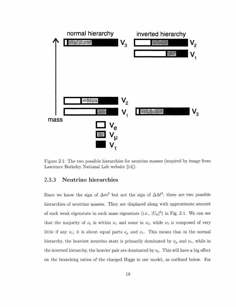
Figure 2.1: The two possible hierarchies for neutrino masses (inspired by image from Lawrence Berkeley National Lab website [14]).

2.3.3 Neutrino hierarchies

Since we know the sign of Am2 but not the sign of AM2, there are two possible

hierarchies of neutrino masses. They are displayed along with approximate amount

of each weak eigenstate in each mass eigenstate (i.e., |£/^|2) in Fig. 2.1. We can see

that the majority of ve is within v\ and some in z/2, while v3 is composed of very

little if any ve\ it is about equal parts v^ and vT. This means that in the normal

hierarchy, the heaviest neutrino state is primarily dominated by v^ and vT, while in

the inverted hierarchy, the heavier pair are dominated by ve. This will have a big effect

on the branching ratios of the charged Higgs in our model, as outlined below. For

19

completeness all the results in this paper have been worked out for both hierarchies.

2.3.4 Mechanisms of neu t r ino mass

Unique among the quarks and leptons, the neutrino is not charged under the EM

or strong interaction. This means that the only way the neutrino can interact with

the other SM particles is though the weak interaction, and thus only the chiral left-

handed neutrino has ever been detected. Also, as seen in the previous section, it is the

SU(2)L x U(l)y symmetry that forbids the other fermions from having a Majorana

mass term. It is thus possible that the chiral left-handed neutrino actually couples

to itself to form a Majorana mass after the electroweak symmetry is broken, and if a

chiral right-handed neutrino exists, it could in fact have a different Majorana mass.

Thus if we want the neutrinos to have only Dirac masses in the same way as all the

other fermions, we must introduce some kind of new symmetry to forbid Majorana

masses.

There is also the problem of how tiny the neutrino masses are. While one can

simply put in small values for the various model parameters that affect neutrino mass

by hand, this seems ad hoc. In the next chapter I will introduce a model that aims

to solve both these problems.

20

Chapter 3

Model

3.1 Introduction

The Standard Model (SM) accounts for almost all the experimental results of high

energy physics; however, the observation of neutrino oscillations is not a prediction of

the model, and thus the model is incomplete. While there are many ways to expand

the model to account for neutrino oscillations, we attempt to do so with the following

goals. First, the neutrino mass scale is significantly lower than the mass scales of

the other fermions, so we would like the model to account for this with the addition

of only one tiny parameter. Second, Majorana neutrino effects have not yet been

observed, so we would like the model to forbid Majorana neutrino masses. Third, we

would like the model to have predictions testable at the LHC.

To this end we expand the SM by introducing a second Higgs doublet ($2)7

in addition to the SM Higgs doublet ($1), as well as introducing three right-handed

spinors VRX, which will be the right-handed components of the three Dirac neutrinos.

21

We then impose a global U(l) symmetry under which the new Higgs doublet and

right-handed neutrinos have charge +1 and the SM fields have charge 0. By breaking

the U(l) symmetry explicitly by introducing a term m\2&\$2 + h.c. in the Higgs

potential, the neutrinos get a Dirac mass proportional to the vacuum expectation

value of the new Higgs doublet (v2). The symmetry still forbids Majorana mass

terms for the neutrinos, and by requiring that v2 be tiny, the Dirac neutrino masses

are suitably small. This model was first introduced in Ref. [1].

In this chapter I give the field content and symmetries of the model, write

down the Lagrangian, derive the physical particles with their couplings, and give the

branching ratios of the charged Higgs H+.

3.2 Field Content

We start with the field content of the SM, and add to it a new scalar SU(2)L doublet

<E>2 (the SM Higgs is renamed $1) and three right-handed gauge-singlets vR% (these

are the right handed neutrinos). Both the SM and new scalar doublet are made up

of 2 complex fields and are written as

$ , = (3.1)

where (4%)* = </>~, and the lower component is written out in real and imaginary

components. The +, —, or 0 superscripts denote the electric charge of the various

fields, determined by the fields' relation to the electroweak symmetries, SU(2)L and

U(l)y. These symmetries restrict the form of the Lagrangian, and if we introduce

any fields into our theory we must give them a charge under the symmetries, i.e.,

22

how they change under the symmetry operation. These charges are conserved in

interactions if the symmetry is unbroken. For the U(l)y symmetry, the charge is

called weak hypercharge and labeled y , and any particular field x w^ change under

the symmetry as

X - e-y*<*>x. (3.2)

The charges associated with SU(2)L are labeled Ta, and since the electro-weak force

is a combination of both symmetries, it turns out that the conserved electric charge

Q that is connected to the strength of the photon coupling is

Q = T3 + | . (3.3)

When fields are placed in a weak doublet it means that the upper field has T3 — \

and the lower T3 — — | . Since we want the upper to have electric charge +1 and the

lower to have charge 0, we know that both </>+ and $ must have Y = 1.

The right-handed vR% are gauge-singlets, i.e., they do not transform under

either the SU{2)L or the U(1)Y symmetry; thus Q = Ta = Y = 0.

3.3 Symmetry breaking

In order to prevent $ i from coupling to the vRx, we impose a new global U(l) sym­

metry under which <J>2 and the three VRX are given a charge of +1 and all the other

fields are uncharged, which leads to a coupling structure of [1]

Cvuk = -yt3dR^\QL3-y:3uR^\QL3

-y[3eR§\LLj - yv%3vR^2Lh3 + h.c, (3.4)

23

where

^ = ia2<S>: (3.5)

is the conjugate doublet and the y's are free parameters of the theory known as

Yukawa couplings.

This Yukawa Lagrangian can also be obtained by imposing a Z2 symmetry

as in the models of Refs. [15, 16]; however, this does not forbid neutrino Majorana

masses.

We want to generate masses for the neutrinos, and as fermions there are two

forms that a mass term can take in the Lagrangain, equations 2.52 and 2.53. This

theory is supposed to forbid Majorana masses, so we check the action of such a

Majorana mass term under the symmetry operation of the new U(l):

-l-m(uR)TCvR - -±m(e-"vR)TCe-"uR = -e^el-m{vR)TCvR. (3.6)

Clearly this term is not allowed by the new symmetry of the theory, which is what

we want.

However, we do want a Dirac mass, so we need a term in the Lagrangian that

looks like

Cm = -mvvLvR, (3.7)

which is also clearly not invariant under the symmetry. To get around this we must

somehow break the symmetry.

There is a similar issue in the SM, where the electroweak symmetries prevent

any masses for the fermions and bosons. That is solved by breaking the symmetry

24

Figure 3.1: A 2-dimensional representation of spontaneous symmetry breaking.

with the SM Higgs boson. The gauge invariant potential for a scalar weak doublet is

V = m2n^i + l^(^i)2- (3-8)

If we define m ^ < 0, then the potential does not have its minimum at the origin.

Imagining it in 2-dimensions, it looks something like Fig. 3.1. To do the perturbation

theory expansion that we use for this type of physics we need to be at a minimum of

the potential, which means picking a position away from the origin, i.e., breaking the

25

symmetry. We can represent this in the Lagrangian by putting in the distance from

the origin we have to go t>i, called the vacuum expectation value (vev), into the field

definition, such that (pt,r is redefined as being at 0 at the minimum:

$ , = \ (vx + <t>0/ + i^l)/V2 J

(3.9)

If we then expand out, for example, the second term in Eq. 3.4, we can see that we

get

& > 1 - V» ,0 .r- -Vx-

£yuk => -VVURMQL,

3 J^-URJLL, - -+(/>{ uRuLj - *-fi<l>i uRuLj + yl3cf)JuRidL3.(3.10)

After diagonalizing the mass matrix M%3 — -yjp we have a Dirac mass term for the

up-type quarks, of mu% = ^-^-. So we see that the mass is proportional to the vev.

We want to do something similar to give a Dirac mass to the neutrino. Since

the neutrino is exceptionally light, we can get a small mass by requiring v2 to be very

small. We could use the same method (spontaneous symmetry breaking) to give the

vev to <&2; however, that leads to undesirable results. The mass of the scalar particles

is correlated to the curvature of the potential. To get a small vev, the curvature

has to be extremely small, and thus we would get scalar particles with masses small

enough to be discovered at energies already probed in experiments. As well, in a two

Higgs doublet system, both Higgs's potentials being broken spontaneously leads to a

massless Nambu-Goldstone boson; this is problematic, as a massless particle would

have been already observed by previous experiments.

There is another way to get a vev for $2- we can break the global U(l)

26

symmetry explicitly. To explain, we look at the potential.

With two Higgs doublets in the theory, the most general gauge-invariant scalar

potential is

V = m2xl^\^i + m2

22§\$2 - \m\2§\§2 + h.c.

+|AX ( V ^ ) 2 + A2 ($f2$2)

2 + A3 ($l$i) ($^2) + A4 ($1$2) (<^$i)

+ [^A5 (<J>i$2)2 + [A6$1$I + A7$J$2] $i$2 + h.c.j . (3.11)

The U(l) symmetry eliminates m\2, A5, A6, and A7. However, we can choose to

give a small non-zero value to the dimension-2 m\2 term; this is the explicit breaking.

This leaves us with a Higgs potential of

V = 771^$}$! + m22$2^2 ~ U i 2 $ l $ 2 + h.C.

+^A1($i$1)2 + ^A2($t2<I>2)2

+A3 ($i$i) ($ f2$2)+A4 ($i$2) ($s$i) (3.12)

So that the local minimum corresponding to the vevs is the global minimum, we

require Ai, A2 > 0, A3 > —VAiA2, and A4 > — \A1A2 — A3. We want to get vi through

the usual spontaneous symmetry breaking procedure, so we need the potential to have

the familiar "mexican hat" shape, which is achieved with m\x < 0. We do not want

the global U(l) to be broken spontaneously as well as explicitly, as that will create

a very light pseudo-Nambu-Goldstone boson, which contravenes standard big-bang

nucleosynthesis (as will be discussed in Sec. 4.1); thus we require the curvature at

the origin m\2 + (A3 + \4)vl/2 > 0. In 2-dimensions, the $ 2 potential looks like Fig.

3.2. Clearly, the size of the vev is independent of the curvature of the potential, so

27

Figure 3.2: A 2-dimensional representation of explicit symmetry breaking.

we can have tiny vev and scalar particles with large mass.

We now can insert the small vev v2 into the Lagrangian and get the mass of

the neutrino in the same way of Eq. 3.10:

£>Yuk D

D

-V^RML^

-•—VR.VL. - -^(f>2 vRivLj - i-^<P2 uRiuLi+yij<i>Zi/RieL., (3.13) yft V2" 'V2C

28

giving the Dirac masses of the neutrinos as

m * = ^ ( 3 - 1 4 )

where the y" are the eigenvalues of the matrix y".

To find the value of the vevs, we must find the minimum of the potential:

dV

d|$ i | dV

d\$2

= m\xvx - m\2v2 + -Xivf + -(A3 + X^Vivl = 0 mm

= m222v2 - m\2vi + -A2^2 + 3(^3 + K)v\v2 = 0 (3.15)

mm

Since m^2 < ^ i , we originally set m\2 = 0 when finding the value of v\. Doing this,

we find the minimum of V with respect to v\ is located at

— 9m2

v\ = - f p l . (3.16)

For v2, we do need to consider m\2, although again we may ignore higher order terms

in —T":

m\2vx V2~m2

22 + l(X3 + X,)v2' [±U)

We will choose parameters so that V\ = 246 GeV and v2 ~ eV.

3.4 Mass eigenstates

To determine the mass eigenstates of fields, we parameterize the mixing with

tan/? = — > 1 . (3.18) v2

29

The mass eigenstates of the charged and CP-odd neutral scalars are given by

G+ = <f>^ sin 0 + 4>% cos 0 ~ (f)f

G° = ^ ' lsin/3 + 02 ' l cos /?~^ ' J

A0 = <f>0{1 cos 0 - 4'1 s i n 0 ^ - 4 ' * , (3.19)

where the Goldstone bosons (G+ and G°), as usual, are massless and do not contribute

as physical particles with the correct gauge choice.

Neglecting contributions of order m22 and v2, the masses are

M2H+ = m2

22 + -X3v2

M\ = m222 + ^(X3 + X4)v

2 = M2H+ + ^X4v

2. (3.20)

The CP-even states also have very tiny mixing of order v2/v\, so h° ~ (f>{r (SM-like)

and H° ~ <jP2T', with masses

MH = m222 + -(X3 + X4)v

2 = M2A

Ml = m2u + ^Xxv

2 = Xlv\. (3.21)

30

3.5 Decays

After diagonalizing the neutrino mass matrix, and going to the Higgs mass basis, Eq.

3.13 yields

£<Yuk = {™>vJvi)lPv%vx - (im^/v^A^v^v,

-{y/2m„Jv2)[Ut%H+D%PLet + h.c], (3.22)

where v% are the mass eigenstates, e is e, /i, or r depending on £, and U& is the PMNS

matrix, as defined in Sec. 2.3.2. Since the decays of H° and A0 to two neutrinos will

be invisible to a collider detector, the decay of most interest is H+ —> £+v.

The charged Higgs can decay into all nine combinations oi£xv3,

T (H+ - t+v%) = H ' 3.23

but, again, because we do not expect to be able to detect the neutrino directly, we

sum over neutrino states and find a decay rate of

r(H+^^) = MH+{™l)\ (3.24)

where we define the expectation value of the neutrino mass-squared in a flavor eigen­

state, {ml)i — X^ 7 7 1^!^! 2 [17]. To simplify the phenomenology, we will work

with the assumption that MHO — M^o > MH+, i.e., A4 > 0, so that the decays

H+ —» W+H°, W+A° will be kinematically forbidden; thus the branching ratios of

the charged Higgs are completely determined by the values of neutrino masses and

31

mixing:

BR(#+ - tv) = J™\ . (3.25)

The overall mass scale of the three neutrinos are unknown; thus all results

are displayed over the relevant range of the lightest neutrino mass, i.e., the range

of the lightest neutrino mass such that it is in the same order of magnitude as the

mass differences. We also display results for both normal and inverted hierarchy. The

branching ratios for the charged Higgs are displayed thus with values obtained by

scanning over the 2a ranges of the neutrino parameters from Table 2.1 in Fig. 3.3.

The large uncertainty in the branching ratios to [i and r is due to the uncertainty in

sin2 #23, a term in the neutrino mixing matrix that mostly affects the mixing between

Vp and vT. Looking back at Fig. 2.1 we can see how the larger branching ratios are due

to weak eigenstates that are concentrated more in massive mass eigenstates. Once

the neutrino masses are much larger than the difference between them, the masses

effectively become degenerate, and thus the branching ratios become degenerate at

1/3.

32

c o ts

c o c CO 1 _ .Q

+ X

c g o co v _

«+—

O) c _c o c co i_

+ X

0 7

0 6

0 5

0 4

0 3

Normal hierarchy

0 001 0 01 0 1

lightest v mass [eV]

0 7

0 6

0 5

0 4

0 3

0 2

0 1

Inverted hierarchy

0 001 0 01 0 1

lightest v mass [eV]

Figure 3 3 Charged Higgs decay branching fractions to ev, /iz/, and rv as a function of the lightest neutrino mass

33

Chapter 4

Phenomenology

In this chapter I present the constraints on our model from big bang nucleosynthesis

and the LEP collider, calculate predictions for JJL and r decay lepton universality tests

and \i —• e7, r —> e7, r —• /ry, and compute the cross section for pp —> H+H~ at the

LHC and compare to the triplet model of Ref. [18].

4.1 Big bang nucleosynthesis

From the amount of helium relative to hydrogen in the universe, we can predict its

early expansion rate (for a review of big bang nucleosynthesis (BBN), see [19]). When

the energy density of the universe is sufficiently high, weak processes such as

ue + n <—> p + e~ (4.1)

maintain the protons and neutrons at chemical equilibrium. However, as the universe

expands the energy density goes down, and at some point this process stops. At that

34

point, the neutrons begin to decay until the universe's energy density becomes low

enough for the neutrons to combine with protons in a 4He nucleus, at which point the

number of neutrons stays approximately constant. By calculating the cross section

of the equilibrium process 4.1 and measuring the ratio of 4He to 1¥L today, we can

calculate what the early universe energy density must have been at various times,

and thus the expansion rate of the early universe [20].

If one postulates the existence of new particles that do not currently interact

with the other SM particles regularly (such as the three new vRx in our model), one

is really postulating a significant amount of new untapped energy in the universe. In

the case of the vRx, they can interact with the SM particles through exchange of the

new Higgs states, e.g.,

VR, +"Rt <—>eLt+eLk. (4.2)

At some point in the early universe, the energy density will be high enough for

this process to happen regularly and make the vRx in thermal equilibrium, resulting

in a whole bunch of extra energy around for which standard BBN theory has not

accounted. This extra energy density would affect the expansion rate of the universe,

hence changing the ratio of 4He to XH. For our model to not contradict the BBN

theory, the extra energy of the vRx must be sufficiently small.

The energy of the vRx will be determined by when they decoupled from the

SM particles. Until that point, their energy is determined by the energy of all the

particles in thermal equilibrium, while after decoupling their energy will be unaffected

by the other SM particles. The energy per particle of the particles in equilibrium in

the early universe actually increases with time: as the energy density goes down,

massive particles, e.g., the bottom quark, can no longer be created, and thus they

decay away and leave all their energy to the remaining particles. Thus to minimize

35

the energy of the vRx we need them to decouple from the SM particles at a sufficiently

early time; i.e., we need the cross section of their coupling to be sufficiently low so

that scattering can only happen at a very high energy density. To discover the limit,

we follow the method of Ref. [21].

The cross section for the reaction in Eq. 4.2 is

_ 1 lmlml aR ~ ^vM^~4lU^ ]Ukl1 E '

where E is the energy of one of either of the incoming neutrinos and v is their

velocity in units of c. If we sum over the various leptons, assuming the mass of all

three neutrinos to be 0.3 eV [22] (assuming neutrinos to have large degenerate mass

gives the strongest constraint), we get a total cross section of

= * l mi £2 7T V M^+V2

In order for our understanding of the rate of expansion of the early universe that

comes from helium abundance to be unaffected by the inclusion of three additional

right handed neutrinos, they must cease to interact once the temperature of the

universe has gone below 40 MeV [19]. Since energy per particle and temperature are

approximately equal, we can write

aR~vMf~^lR>

where TR is the temperature of the right-handed neutrinos. The similar interaction

36

for left-handed neutrinos (mediated by a W boson) has a cross section

vMi rrr ~ 1-Z—T2

aL ~ — A l j Li W

where g is the weak coupling constant, and has a decoupling temperature of ^ 3 MeV

[19]. We will use the ratio of the two cross sections so that we can cancel out the

dependence on the expansion rate of the universe later.

The rate of the reaction is related to the cross section by Y = ne < av >, where

ne is the number density of the leptons and < av > is the cross section averaged with

the velocity distribution. Because ne oc T3 [20], we obtain

4

and a2

_y_ rpb M 4 L' 1V1W

Decoupling happens when the reaction rate drops below the expansion rate of the

universe. Since the universe's expansion rate is t~~l ~ T2, at decoupling we have

m TR OC -T^-ATR, (4-3)

R M%+v\ R' K '

and

and we can take the ratio to get

n«&n («) LW

37

where now we have placed the decoupling temperatures required for the neutrinos

to not contravene what we know about the early universe from helium abundance.

Using MH+ « Mw, mv « 0.3 eV, g « 0.7, TdL w 3 MeV, and TdR > 40 MeV, we get

v2 > 3 eV.

This can also be expressed as a limit on the couplings,

y!; = V2mJv2<0.1. (4.5)

As desired, this Yukawa coupling is not too tiny; this limit is the same order as the

bottom quark Yukawa coupling in the SM.

4.2 Tree-level muon and t au decay

In the SM, the lifetime of the tau lepton rT can be written in terms of the muon

lifetime r^ as

and

^p2m5 "^ f{m2/m2T)rr

Rc

where /(x) = 1 — 8x + 8x3 — x4 — 12xln(x) is a phase space factor, rRC represent

electromagnetic radiative correction factors, and g2/g2 = g2ej'g

2 — 1 are the charged

current coupling constants [23]. If we add new decay modes for the muon and tau,

the equation will still hold, but the charged current couplings will no longer be equal

to unity.

38

In the Higgs doublet model, both muon decay and tau decay can be mediated

by a charged Higgs boson, as well as by the SM method of a W boson, leading to an

additional decay width of

m5

r " " = 12(47r)3M£+v4 <m'>*. < m ^ , ' LH+

(neglecting final state masses) where £% and £f are the initial and final lepton in

the decay process, and (ml)£ = ^2lml\Uel\2. The two mechanisms for decay do

not interfere because the neutrinos in W~ mediated decay are left-handed, while the

neutrinos in H~ mediated decay are right-handed. This leads to charged current

couplings of gl l + (2GFM2

H+v2)-2(ml)li(ml)e

g2 l + {2GFM2H+v2)-2{ml)T(ml):

and

gl 1 + (2GFM2H+v2)-2 {ml)T K ) „

9* 1 + (2GFM2H+v2)-* (ml)T (m*),'

where Gp — \[2g2/8M^/V is the Fermi constant. The current experimental values

of the charged current coupling ratios are g^/gT — 0.9982 ± 0.0021 and g^/ge —

0.9999 ± 0.0020, and this is displayed graphically versus different values of v2 in

Figures 4.1 and 4.2. As can be seen, the BBN requirement that v2 > 3 eV means that

9H/9T a n d g/j,/ge are well within the expected limits and thus provide no additional

constraints.

39

v2 [eV]

3. 1 000

v2 [eV] (a) (b)

v2 [eV] (c)

v2 [eV] (d)

Figure 4.1: Values for the charged current coupling constants (showing the two sigma experimemtal limits) versus v2, with the mass of the charged Higgs set at 100 GeV (a larger charged Higgs mass will result in a lower constraint) and normal hierarchy neutrinos with a smallest mass of (a) and (b) 0 eV, and (c) and (d) 1 eV.

40

v2 [eV] (a)

v2 [eV] (b)

v2 [eV] (c)

v2 [eV] (d)

Figure 4.2: Same as Figure 4.1 but with inverted hierarchy neutrinos.

41

4.3 LEP-I I constraints on H+ mass

The CERN Large Electron-Positron (LEP) collider experiments looked for supersym-

metric (SUSY) partners of the SM leptons via the reaction

e-e+ _+ i+t _> e+xlrxl

where £ is a charged slepton and Xi the lightest neutralino, which essentially means

looking for a lepton, its antiparticle and some missing energy. In our model, the same

observable particles would result from

The LEP experiments give the limits on the cross section of the SUSY process versus

the mass of the sleptons and the neutralinos [24]. We can use the mass of the sleptons

to stand in for the mass of the if+; the limits will be analogous as the sleptons and

charged Higgs have the same spin, and thus the kinematics will be identical. The

results are plotted versus the mass of the neutralinos in GeV, and on that scale, we

clearly want to take the mass of the neutralino as 0, which in our case stands as the

neutrino. The LEP results are quoted for the final state of e+e~p™lss and //+^~p™ss,

and I used both to determine lower bounds on M#+.

To compare to our model, we computed the leading order parton level cross

42

section for charged Higgs production for various values MH+:

KJ ' 48irNc V s )

X \ s2 + (s- M2Y {9v + 9A)

2e2Qfg2(TH+-s2

w) \ + 8(8 ~ M\) 9V) ' ( 4 ' 6 )

where Nc is the number of colours (3 for quarks and 1 for leptons), e is the electric

charge constant, gz — e/(sin 9w cos 9w), where 9w is the weak mixing angle, sw =

sm9w, Qf is the fermion electric charge in units of e, TH+ is the 3rd component of

weak isospin of the charged Higgs (1/2 for the doublet Higgs model of this paper),

gv — Tf/2 — QfSw, where Tf is the 3rd component of weak isospin of the fermions,

gA = Tf/2, and s = (Ef + Ej)2 is the collision center-of-mass energy squared.

The charged Higgses were then decayed using the branching ratios that would

give the most conservative result, which is the 2a lower bound (see Fig. 3.3 for branch­

ing ratios).

The lower limits on the mass of the charged Higgs that result from this analysis

are displayed in Figure 4.3.

4.4 Decay ra te of L —> ^7

With the existence of a charged Higgs boson, flavour-violating decays can occur where

a charged lepton decays to a lighter one and a photon:

L -* £j, (4.7)

43

e_z/ee+z/e

60 70 80 90

mH+ [GeV] (a)

e Z/ee+i/e

mH+ [GeV]

(b)

Figure 4.3: Limit on mass of charged Higgs for various values of the lightest neutrino mass for (a) normal hierarchy and (b) inverted hierarchy.

where (L,£) — (r,//), (r,e) or (/i, e). This process can also occur in the SM via the

W, but the rate is exceptionally small (BR(^ —> e7) < 10~40, see Ref. [25]).

The possible first order diagrams for this process are displayed in Fig. 4.4; we

treat the final state electron as a massless particle throughout the calculation.

The amplitude for this process can always be written as the Lorentz structure

[26]

iM = e'Jq)us'(p')[A'f + Bi<Ti»'qu]ua(p). (4.8)

In this case we end up with

A = 0, (4.9)

44

H~ . . - /

/ H~

M P i/,(fc) p' e~

(a)

H~

V V p' Ul(k) p' e"

(b)

A»" P !/,(*) P p' e"

(c)

Figure 4.4: The three possible first-order Feynman diagrams for /i charged Higgs.

B = M

J2<UvU«P*>

e 7 via

(4.10) 6v2M2

H+(^)2

where PR = (1 + 75)/2 is the right projection operator. This result agrees with

that of Ref. [27]. Term B is entirely from diagram (a), while (b) and (c) can only

contribute 7M terms, which cancel with the 7M term from (a) (for the full calculation,

see Appendix A).

We average over initial spins and sum over the final state spins and polariza­

tions to get

9 /_j I I

1 e2 m\

ss'pol 36(4TT)4 V\ Mf,

H+ £ mlU*xUex (4.11)

Since we are ignoring the mass of the electron, we substitute this into the

formula for decay to two massless particles,

r = -±-ly\M\ ^ ss'pol

m" 144(4TT)5M£+ V\ E<u*u°

(4.12)

(4.13)

The decay from r to ji or e is the completely analogous equation, so we sub-

45

stitute [i —> L and e —> £ to get the general result. To put this in a form that

is more useful, we make use of the fact that T(L —> evv) ;» T(L —• ^7), where

G2Fmj

1927T3 T(L ^ eisv) = %gt [28], to write

BR(L->*y) - B R ^ L ^ e ^ f | r ^ l ) (4-14)

= B R ( L ^ C wfe 2^A^4 ' ( }

where aem — e2/47r and G^ is the Fermi constant. This is the form presented in

Ref. [1]. Due to the factor of ^ rn2UjjlUil\ in the branching ratios, there is a large

dependence on the neutrino parameters. The various branching ratios have been

plotted against some parameters with large effects in Fig. 4.5.

For MH+ = 100 GeV and v2 = 3 eV, BR(/i -* ej) < 2 x 10~12. The current

experimental 90% CL upper limit for muon decay is BR(^ —> e7) < 1.2 x 10 -11 [29],

above our branching fraction. However, for certain values of the neutrino parameters

this decay rate could be observed at the MEG experiment after running to the end

of 2011, which expects to have sensitivity to 10 -13 [30].

Similarly, for MH+ = 100 GeV and v2 = 3 eV, BR(r -> e*y) < 2.5 x 10~13 and

BR(r —• ^7) < 4.5 x 10~12. These are also below the current 90% CL bounds from

BABAR of 1.1 x 10~7 [31] and 6.8 x 10"8 [32] respectively. This is also below the

future prospects of the SuperB next-generation flavor factory of 2 x 10 -9 in either

channel [33].

46

ST

t

CL CO

"T ' — ' — ' ' ' ' ' 1

r

T

*H

l

MEG

Pr

target !

-

-

-i_U 1

sine.,

(a)

CC 2 5e-12 OQ

ST

t

of CD

(b)

0 0016 0 0018 0 002 0 0022 0 0024 0 0026 0 0028 0 003

AM2 [eV2]

(c)

Figure 4.5: Branching ratios for L —> £7 plotted against neutrino parameters with large effects, for MH+ = 100 GeV and v2 = 3 eV. In all cases the normal hierarchy is used, as the inverted hierarchy plots are similar. In (a) the expected limit from the MEG experiment after running to the end of 2011 [30] is plotted, and it is apparent that for certain values of neutrino parameter space the effects of the model would be noticed.

4.5 Charged Higgs pair product ion at LHC

Equation 4.6 gives the cross section for charged Higgs pair production if we start

with two fermions with known momentum. At the LHC, however, we start with

protons of well defined momentum, but the partons inside the protons (quarks and

47

gluons) collide with only some fraction of that momentum. The probability of finding

a particular parton with particular momentum fraction is encoded in the parton

distribution functions.

4,5.1 Parton distribution functions

In the case of the LHC, there will be two protons colliding with a known center of

mass energy, planned to be 14 TeV. However, this is not all the information we need,

as the protons are composite particles, and it is the fundamental particles contained

within them that annihilate each other to create new particles. While a proton is

commonly known to be made up of two up-type quarks u and a down quark d, there

are QCD processes constantly underway inside, and thus there is a finite chance that

when the protons collide, the fundamental particles that collide may be any type

of quark, anti-quark or gluon. As well, while the momentum of the entire proton

is well known, the fraction of that momentum carried by the fundamental particles

can vary dramatically. These two probabilities (of hitting a certain particle and its

momentum) are functions of the center-of-mass energy of the collision. This function

is called a parton distribution function (PDF).

The function is written as fq/p(x), where q is the parton in question, and x is

the momentum fraction. Thus if I want to find the total cross-section of the signal

process pp —> H+H~, I need to sum up the partonic cross-sections of the quarks and

gluons that could collide in the accelerator. I also need to integrate over the range

of the momentum fractions they could have, since the partonic cross-section will be

a function of the collision energy y/I of the partons, not the constant collision energy

48

yfs of the protons:

a(pp -> H+H~) = V / dxx [ dx2a(qq -> # + # " , s)/*/P(xi)A/P(x2), (4.16)

where s = Xix25 and yfs — 14 TeV.

The theory of how the insides of hadrons work is not well understood, as it

cannot be understood through perturbative QCD, so PDFs are constructed by fitting

to as much experimental data as possible. PDFs are only valid at CM energies far

greater than the mass of the partons [34].

There are several collaborations working on preparing sets of PDFs, and they

are updated regularly as new experimental results and theoretical tools become avail­

able. In this calculation, the CTEQ6 PDFs were used [35].

4.5.2 Comparison to triplet model

Because of its dependence on T#+, the H+H~ cross section in Eqs. 4.6 and 4.16

provides an important measurement of the isospin of the charged Higgs. This is

particularly useful for distinguishing our doublet Higgs from the isospin triplet Higgs

of Ref. [18]. We calculated the leading-order (LO) and next-to-leading-order (NLO)

cross-sections for the production of an H+H~ pair at the LHC using PROSPINO [36, 37]

for both the doublet Higgs model presented in this paper and the triplet Higgs model

of Ref. [18] (more will be said about NLO calculations in Sec. 5.6). Results are shown

in Fig. 4.6. The difference is due entirely to the difference in the weak hypercharge

of the charged Higgs: +1/2 for a Higgs weak doublet and 0 for a Higgs weak triplet.

This difference in production rate is essential for identifying the correct model, as the

49

triplet charged Higgs has identical branching ratios to that of our model.

The theory uncertainty on the NLO H+ H~ cross-section has been variously

quoted as 15% [38] to less than 25% [37]. We find that the cross section for H+H~

for our model is 2.7 (2.6) times larger than in the triplet model for M#+ = 100

(500) GeV.

50

n 1 r doublet LO -

doublet NLO triplet LO •

triplet NLO «•

100 150 200 250 300 350 400 450 500

mH+ [GeV]

4.6: LO and NLO production cross-section at LHC (14 TeV) for charged Higgs

51

Chapter 5

LHC signal/background study

5.1 Introduction

In most other models with a charged Higgs, the charged Higgs decay rate to a partic­

ular charged lepton is proportional to the square of the mass of the charged lepton.

Thus such a charged Higgs decays predominantly to the heaviest lepton, the r, which

is much more difficult to detect in a collider than the lighter charged leptons: while

the electron and muon are detected directly, the tau will decay before it reaches a

detector, and thus must be pieced together from its decay products. In our model,

however, the charged Higgs decay rate is proportional to the neutrino masses and

mixing: specifically, the expectation value of ml in a flavour eigenstate. Since mass

eigenstate v3 contains approximately half the ji interaction eigenstate, while V\ and

v2 of similar mass contain virtually all of the e state, regardless of the hierarchy of

the neutrinos, there will always be a decay to e or ji with a sizable rate. With this

in mind, as well as the high rate of both e and \i identification, we look for a process

to study at colliders with either of these charged leptons in the final state. In the

52

interest of picking the most distinctive signature, we will examine pair production of

charged Higgs, mediated by a photon or a Z boson, with a final state of a charged

lepton and charged anti-lepton with missing transverse energy.

To determine if the model can be detected, we note that the decay of the

charged Higgs (H+) to only charged leptons and neutrinos, with branching ratios

determined by the neutrino mixing parameter, is fairly unique. To determine if the

additional rate of charged leptons caused by the H+ decay is noticeable at the LHC,

we used MadGraph/MadEvent v4 [39] to generate signal (H+H~ -> ££'pfss; ££' =

e + e - ^ V , ^ / ^ ) and background (VV -> ££fpfss; V = W,Z, or 7; and it - •

££'PTISSJJ, j — jet) events. With appropriate cuts, it was determined that 5a discovery

statistics can be achieved with luminosity in the range 6-50 fb""1 for MH+ = 100 GeV,

depending on the neutrino mixing parameters. For MH+ = 300 GeV the minimum

luminosity for 5a discovery statistics is 200 fb -1.

There will be background processes with final states that are or appear to be

the same as the signal. Thus we will examine the kinematic features of the signal and

the background to determine selection cuts that will minimize the background while

allowing as much of the signal to still get through as possible. We then examine the

signal significance, which we do with Monte Carlo techniques. Our goal will be to get

to a significance of 5<r, which is the significance conventionally required in particle

physics to claim discovery.

5.2 Monte Carlo simulations

Having determined the best way to test the model at the LHC, it is desirable to know

whether it will, in fact, be observable. To do so we simulate the collider environment

53

on the computer with a Monte Carlo simulator: this is the method of turning random

numbers into a database of simulated events. To do this, we need to know the

probability of events of various types occurring in the experiment. There are several

steps to figuring this out, outlined in the following. The overall software package that

was used for all these steps is MadGraph/MadEvent v4 [39].

5.3 MadGraph/MadEvent

MadGraph uses PDFs as described in Sec. 4.5.1; in our simulation, we specified

the CTEQ6 PDFs [35]. Next we need to know the probability of the processes we

are interested in happening. This requires calculating the amplitude for the various

Feynman diagrams that contribute to a desired process. For example, the tree-level

diagrams for the process uu —> H+H~ —» e~ve\irv^ are displayed in Fig. 5.1.

While one could figure what all the diagrams are by hand, there are computer

programs that have been designed to do so, such as MadGraph which was used for

this simulation. MadGraph creates all the tree-level Feynman diagrams for a given

process by generating all possible topologies for a tree-level process, and then assigns

the particles requested by the user, checking the Feynman rules to see if the vertex

is allowed, before finally adding the symmetry and colour factors to the diagrams

[40]; Fig. 5.1 is part of the output of MadGraph. The default particle theory model

MadGraph uses is the SM, but it has built in several other common models, and we

were able to modify the default two-Higgs-doublet model with our couplings.

MadGraph then constructs a program using the subroutines of another soft­

ware package, HELAS (HELicity Amplitude Subroutines), for computing the helicity

amplitudes of tree-level diagrams numerically [40]. At this stage, we have the calcu-

54

Diagrams by MadGraph u~ u -> e- ve~ mu+ vm

- " he

[6

-..he

graph 1

mu vm

- - he

.he

graph 2

mu ym

- h e

..he

graph 3

mu ym

graph 4

graph 5

Figure 5.1: The tree-level Feynman diagrams for the process uu e~Pe/x

+^, produced by MadGraph.

55

lation tools required to make simulated events.

Once the amplitudes have been identified, they must be integrated over phase-

space; this is done with MadEvent using Monte Carlo techniques. It is a non-trivial

task, as one does not want a probability distribution that samples all of phase space

evenly, since the amplitude will in general have sharp peaks in some areas that need

to be examined with higher density. These peaks can usually be surmised directly

from the form of the Feynman diagrams, as they usually arise from the propagators

approaching collinear-divergent limits or when virtual massive particles with small

mass are close to their mass shell [41]. It is thus MadEvent's job to identify these

peaks and create a random sampling of the phase space that is tailored to the shape

of the amplitudes.

One of the results of this method is that the events it produces at first tend

to be weighted. For example, if 10,000 events are created, and there is a large area of

phase-space where an event would only be found at a rate of 1/20,000, a representative

event will be created but will be weighted as 0.5 of an event. This results in smoother

histograms. There is also the option to create unweighted events, which forces the

program to choose whether there is a full event in a region of phase space or not. For

this simulation, unweighted events were used.

5.4 PYTHIA-PGS

MadEvent is a parton level Monte Carlo, so the results were passed through a

PYTHIA-PGS package designed to be used with MadEvent. The events MadEvent

creates can have quarks in the final state (our tibackground has bb in the final state),

and in reality any quarks will quickly hadronize due to quark confinement and create

56

jets. PYTHIA [42] is a software package designed to as accurately as possible simu­

late the hadronization process. As well, events in reality will have low energy initial

and final state radiation from any external quarks or gluons, and PYTHIA simulates

this as well.

To make the simulation more realistic, there is an attempt to simulate the

experimental apparatus itself. Specifically, different detectors have different levels of

accuracy. Certain particles are more likely to be detected correctly, if at all; even if

a particle is detected, the accuracy of the trajectory and energy measurement varies

between particle species as well. While there are very detailed detector simulations

that take into account the physical location of all the material used in the LHC

detectors, this is only a feasibility study, so the basic detector simulator PGS (Pretty

Good Simulation) [43] was employed (the default settings for ATLAS were used).

We have provided the cut efficiencies from a parton-level (no PYTHIA/PGS)

simulation for ease of comparison, along with the full PYTHIA/PGS simulation.

5.5 Signal and Background Processes

The LHC signature is pp •-> H+H~ -> lvit!vii, with ££' = e+e~, p+ft', e*1 fjF. The

relevant backgrounds to this process are pp —» VV —> Ivtlv (with V = W, Z, or 7

and the neutrinos can be of any type), and pp —> ti —> £vt£'vt>bb\ the ti process is

important because of the exceptionally high rate of top quark pair production at the

LHC.

The di-vector boson background is included as it is the only tree-level process

to produce the same final state as the signal in the SM. While the ti background

57

has a different final state, it has such high cross section at the LHC that even after

cutting out the events with a detectable jet, there will still be a significant number of

events. We cannot throw out all events with any jets, as there will often be soft jets

in signal events from other partons, and there will also be soft jets from the tt events

that will not be noticed by the detectors.

The default number of events MadGraph simulates is 10,000. All the simula­

tions were run with this number of events with the exception of the ti background,

which was run with 100,000 events because we needed to have smaller granularity on

such a large background.

The branching ratios (BR) for the charged Higgs, displayed in Fig. 3.3, are de­

pendent on the neutrino masses, and thus depend on as-yet-unknown neutrino sector

parameters. For small neutrino mass, the normal hierarchy leads to approximately

equal branching ratios to \i and r, and none to e, while the inverted hierarchy leads

to a branching ratio of ~0.5 for e and again approximately equal branching ratios to

[i and r of ~0.25. In both hierarchies, as the mass of the lightest neutrino increases,

the branching ratios become more degenerate, until they converge to 1/3 at around

mu ~ 0.5 eV. For the background, the default branching ratios of the W and Z from

MadGraph were used. They are,

• BR(W+ -> £+v£) = 0.10680

• BR{Z -» l+tr) = 0.03360

• BR(Z -> vv) = 0.20000.

We assume BR(£ -> W+b) = 1.

58

5.6 Q C D Correct ions

Doing the calculation with only the tree-level diagrams (diagrams with no closed

loops) is known as a leading-order (LO) calculation. At tree level, our processes have

only electroweak vertices, but we can also calculate diagrams with one (pp —> H+H~j,

where j is a jet), or two (pp —• H+H~ one-loop) quantum chromo dynamics (QCD)

vertices; this is called the next-to-leading order calculation (NLO) in QCD. Depend­

ing on the process, this correction can have a varying impact, but for electroweak

processes is frequently in the area of 30%.

We wish to incorporate QCD NLO results into our simulation for two reasons:

first, we want more accurate cross-sections, but also, since we use a jet-veto to lower

the ti background, we need to investigate the effect this cut will have on our signal

process with a final state jet, which is part of the NLO process.

As mentioned above, MadGraph is a tree level event generator, so in order to

get a more accurate simulation, NLO results were incorporated as follows.

First, we found the total NLO cross-section for the signal and backgound

processes. The NLO cross-section for pp —> H+H~ at the LHC was calculated using

PROSPINO [36, 37] with CTEQ6 [35] parton densities, with the renormalization and

factorization scales equal to MH+.

The NLO cross-sections for SM background processes were obtained from Ref.

[44] for the vector boson mediated process. The paper quotes results using both the

MRS98 and CTEQ5 PDF sets, with results differing by 6%. For consistency, the

results using the CTEQ5 PDF were used, as the MadGraph events were generated

using the similar CTEQ6 PDF. For events with both a \i and e in the final state, only

the cross section for W + iy~ is relevant; for events with //+/i~ or e+e~ in the final

59

state, both the V^+jy and ZZ mediated processes contribute, and thus the NLO

cross-section is slightly larger.

The top quark pair production rate at the LHC was taken from Ref. [45],

which calculates the contribution from both NLO and next-to-leading logarithmic

(NLL) terms. The NLL calculation takes into account the first two logarithmic terms

in all orders of the QCD coupling. There is a theoretical uncertainty of about ±5%

when the factorization and renormalization scales are varied between mt/2 and 2mt.

The relevant cross sections are, at NLO/NLL,

• for MH+ = 100 GeV, a(pp - • H+H') = 295 fb

• for MH+ = 300 GeV, a(pp -> H+H~) = 5.32 fb

• a(pp - • W+W-) = 127.8 pb

• a(pp - • ZZ) = 17.2 pb

• a(pp —> ti) — 833 pb.

Normally, to change the tree level Monte Carlo results to NLO results, the

tree level results would be multiplied by a A;-factor determined by the ratio of the

tree-level and NLO cross-sections before cuts. However, in order to suppress the top

quark pair production background, we will apply a jet veto, and this cut will affect

tree level events (which have no jet) and NLO events (which can have final state

radiation jets) differently; thus an attempt must be made not only to scale results to

the overall cross-section of the NLO events, but to incorporate the jet structure of

the NLO events as well.

This was accomplished by running a MadGraph/MadEvent simulation for

H+H~ and VV processes of not just the desired tree-level process, but also the

60

similar process with an extra jet in the final state (where a jet could be any quark or

a gluon). Since there is a singularity in the calculation for this process as the energy

of the jet approaches zero, a minimum px cut of 10 GeV was applied at the event

generation level. The equation for the NLO matrix element is

\M\2NLO = \MLO + M^oorf + \M\l_jet. (5.1)

We have calculated the corresponding cross-sections for MLO and M\-3et in MadE­

vent, and have either calculated the cross-section for MNLO using PROSPINO or taken

it from the literature as discussed above. We find that with our minimum PT cut

on ai-jet, aNLO < &LO + &i-jet, so it must be that the 1-loop diagrams decrease the

cross-section, and thus the contribution from the LO process must be scaled down,

in order to incorporate the effects of the 1-loop correction.

For the parton level calculation, the relevant scale factor is determined by,

before cuts are applied, solving the equation

°NLO = kaLO + ai_jet (5.2)

for fc, and then using this equation with the same value of k to calculate a^LO after

the cuts are applied to LO and 1-jet MadEvent simulated results.

For the PYTHIA-PGS calculation, the simulated events have extra jets pro­

duced by PYTHIA and smearing of the detected jet PT, SO instead the equation has

two constants:

VNLO = ma% + nac^jeV (5.3)

where <T£Q is chosen to contain no jets with pT > 10 GeV, and af^ t has at least

61

Cut name Explanation Basic cuts Present are a lepton and antilepton, both with pi > 20

GeV. Also, p%lss > 30 GeV. For parton level, there is cut applied so that \rje\ < 3.0 and 1 1 < 2.4.

Jet veto Designed to reduce ti background, any event with a jet of p3^ > 30 GeV was cut. For parton level, the veto is only applied when \r]3et\ < 5.0.

Z pole veto To eliminate events that include Z —> £+£~~, we veto events with the invariant mass of the two leptons be­tween 80 GeV and 100 GeV (applied only to e+e^p™ss

and /x+/i~p™ss final state events). H'T cut To eliminate the background mediated by W/Z/j, we

make use of the mass difference of these particles ver­sus if+, and also the spin difference of these particles (1) versus H+ (0). It was found that the best way to accomplish this was to cut on H'T = p£

T + p? +p™lss. For MH+ = 100 GeV, we require H'T > 200 GeV, and for MH+ = 300 GeV, H'T > 600 GeV.

Table 5.1: The cuts applied to the simulated data to get the cleanest signal.

one jet with pT > 10 GeV as identified by PGS. a£^ is chosen from the parton-level

aLO after it has run through PYTHIA-PGS and af^jet is chosen from the parton-level

a^et after it has run through PYTHIA-PGS.

The constants m and n are determined by maf^ = kaLo and naf^jet = ai-jet

with k from Eq. 5.2. Equation 5.3 with the same values of m and n is then used to

calculate aNLo after the cuts are applied to the PYTHIA/PGS simulated events.

5.7 Selection Cuts

Four cuts were applied to the simulated data to get the cleanest signal, and they are

explained fully in Table 5.1.

The first cut simply checks for the signal final state. We look for ££', where

62

££! = e+e~, /x+/i~, or fi+e~ depending of the channel we are simulating (^~e+ was

not simulated; instead the /x+e~ luminosity was doubled in significance calculations).

Both leptons are required to have a momentum of greater than 20 GeV so that they

are from an event of high energy. We also look for the neutrinos by requiring the

missing transverse energy (p™ss) to be greater than 30 GeV. For the parton-level

simulation, we put cuts on the pseudo-rapidity (77 = — log[tan(0/2)], where 9 is the

angle away from the beam axis) to simulate the acceptance of the detectors. In the

case of the PYTHIA-PGS simulation, the detector acceptance is taken care of by

PGS.

Next a jet veto is applied at 30 GeV, which eliminates at least 97% of the cross-

section of the ti backgound. For the parton level simulation, the cut is only applied

to jets with \qjet\ < 5.0; for the PYTHIA/PGS simulation, PGS only registers jets

with \r)jet\ < 5.0, so the jet cut is applied to all events. Notice that when NLO is

taken into account, around half of the signal cross-section is eliminated by this cut.

A Z pole veto is applied (veto on 80 GeV < ^Jpt • pi< < 100 GeV) to the e+e~

and ji+fi~ final state events to eliminate any background that results from a Z boson

decaying to two leptons. This will also eliminate the majority of any background

from Z + jets with fake p™lss, which we did not simulate.

The final cut is a cut on H'T = plT -\-pl

T + p™lss, designed to cut down on di-

boson background by making use of the mass and spin differences between the electro­

weak bosons and the charged Higgs. For MH+ = 100 GeV, we require H'T > 200 GeV,

and the signal is cut by ~35% while the di-boson background is cut by ^85%; for

MH+ = 300 GeV, we require H'T > 600 GeV, and the signal is cut by ~50% while

the di-boson background is cut by ~99.5%.

63

The cut efficiencies on ajsrLO for the signal and background for the process

pp —> e+e~p™zss are displayed in Tables 5.2 and 5.3. Efficiencies for the process pp —>

/x+n~pjtlss are displayed in Tables 5.4 and 5.5, and for the process pp —> e±/jJTp™'lss

in Tables 5.6 and 5.7.

Cuts Basic cuts Jet veto Z pole veto H'T cut Cumulative

MH+

Parton 0.62644 0.68348 0.90867 0.65932 0.25651

= 100 GeV PYTHIA/PGS

0.47868 0.60885 0.89900 0.65790 0.17238

MH+

Parton 0.92961 0.57623 0.97783 0.50051 0.26216

= 300 GeV PYTHIA/PGS

0.72128 0.45466 0.97763 0.48794 0.15644

Table 5.2: Cut efficiency for pp —» e+e~p™lss via H+H~. The efficiency of each cut is calculated as the number of events that passed the cut divided by the number of events that passed the previous cut. The cumulative efficiency is the number of events that pass all the cuts divided by the original number of events. Recall, H'T > 200 GeV for MH+ = 100 GeV, and H'T > 600 GeV for MH+ = 300 GeV.

Cuts Basic cuts Jet veto Z pole veto H'T > 200 GeV H'T > 600 GeV Cumulative for H'T

Cumulative for H'T

> 200 GeV > 600 GeV

VV Background Parton 0.42419 0.65626 0.73839 0.16947 0.00221 0.03484 0.00045

PYTHIA/PGS 0.31927 0.62606 0.73374 0.15039 0.00167 0.02206 0.00025

tt Background Parton 0.58407 0.01252 0.90834 0.54669 0.00904 0.00363 0.00006

PYTHIA/PGS 0.40834 0.02856 0.86707 0.42829 0.00198 0.00433 0.00002

Table 5.3: As in Table 5.2 but for background for pp —> eH e pT .

64

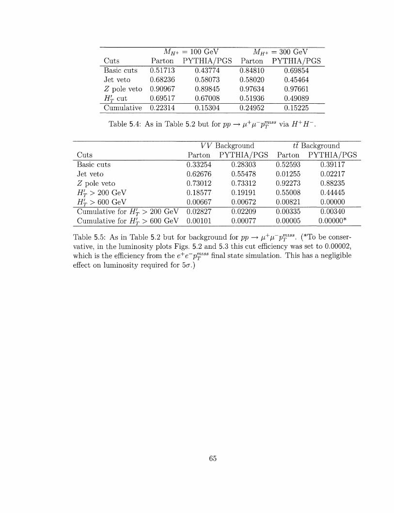
Cuts MH+ = 100 GeV

Parton PYTHIA/PGS MH+ = 300 GeV

Parton PYTHIA/PGS Basic cuts Jet veto Z pole veto H'T cut Cumulative

0.51713 0.68236 0.90967 0.69517 0.22314

0.43774 0.58073 0.89845 0.67008 0.15304

0.84810 0.58020 0.97634 0.51936 0.24952

0.69854 0.45464 0.97661 0.49089 0.15225

Table 5.4: As in Table 5.2 but for pp -> //+//~Pr™ via H+H-

Cuts VV Background

Parton PYTHIA/PGS tt Background

Parton PYTHIA/PGS Basic cuts Jet veto Z pole veto H'T > 200 GeV H'T > 600 GeV

0.33254 0.62676 0.73012 0.18577 0.00667

0.28303 0.55478 0.73312 0.19191 0.00672

0.52593 0.01255 0.92273 0.55008 0.00821

0.39117 0.02217 0.88235 0.44445 0.00000

Cumulative for H'T > 200 GeV 0.02827 0.02209 0.00335 Cumulative for H'T > 600 GeV 0.00101 0.00077 0.00005

0.00340 0.00000*

Table 5.5: As in Table 5.2 but for background for pp —»• n+n~p™tss. (*To be conser­vative, in the luminosity plots Figs. 5.2 and 5.3 this cut efficiency was set to 0.00002, which is the efficiency from the e+e~p™iss final state simulation. This has a negligible effect on luminosity required for 5a.)

65

MH+ = 100 GeV MH+ = 300 GeV Cuts Parton PYTHIA/PGS Parton PYTHIA/PGS Basic cuts Jet veto H'T cut Cumulative

0.56131 0.68783 0.64561 0.24926

0.45765 0.59530 0.63288 0.17242

0.88249 0.57524 0.50134 0.25451

0.70832 0.44956 0.50590 0.16109

Table 5.6: As in Table 5.2 but for pp ->• e±^p%iss via H+H~.

Cuts Basic cuts Jet veto H'T > 200 GeV H'T > 600 GeV Cumulative for H'T

Cumulative for H'T

> 200 GeV > 600 GeV

VV Background Parton 0.35296 0.66428 0.14731 0.00255 0.03454 0.00060

PYTHIA/PGS 0.28171 0.60830 0.12916 0.00245 0.02213 0.00042

tt Background Parton PYTHIA/PGS 0.55297 0.39747 0.01255 0.02624 0.52161 0.39597 0.00865 0.00000 0.00362 0.00413 0.00006 0.00000*

Table 5.7: As in Table 5.2 but for background for pp —> e±/jJTp™'LSS. (*To be conser­

vative, in the luminosity plots Figs. 5.2 and 5.3 this cut efficiency was set to 0.00002, which is the efficiency from the e+e~p™lss final state simulation. This has a negligible effect on luminosity required for 5a.)

To look at the PYTHIA/PGS results after the cuts, the e+e~ channel will

be used as an example. Assuming approximately degenerate neutrino masses, for

which the charged Higgs branching ratios are 1/3 for all three modes, the signal for

MH+ = 100 GeV in the e+e~ channel goes from 32.8 fb before cuts to 5.65 fb after

cuts, the di-boson background goes from 1570 fb to 34.7 fb, and the ti background

goes from 9500 fb to 41.1 fb, resulting in a signal over background of 0.075; in the

case of MH+ = 300 GeV, the signal over background is 0.158.

After cuts, the cross-section of the smaller signal process (MH+ = 300 GeV) is

M).l fb. The cross section due to top pair production before cuts in our final state of

interest is ~10 pb. If only 10,000 ti events are generated, each event represents ~1 fb

of cross-section, too large for an accurate assessment of signal over background. To

66

address this, 100,000 events were run of each top-pair process, so that each simulated

event corresponds to ~0.1 fb. When the cuts are applied, in certain cases, no ti events

get through, which could be cause for concern; however, in the simulation with final

state e+e~p™lss, two events do get through, and the resulting significances are not

noticeably different from the simulations in which no ti events pass the cuts. Thus,

it seems reasonable to simulate this number of ti events. For the other background

processes, 10,000 events were generated, leading to a cross-section per event of ~0.1

fb. The signal was also generated with 10,000 events.

The luminosity required for a 5a discovery of H+ is displayed in Fig. 5.2 for

MH+ = 100 GeV, for each channel separately and for all three channels combined,

and in Fig. 5.3 for MH+ = 300 GeV. For the normal hierarchy with MH+ = 100 (300)

GeV, we find 5a discovery statistics with a minimum of 6 (184) fb - 1 of data at 14

TeV beam energy. For the inverted hierarchy, the minimum is 6 (275) fb -1 of data,

and for the degenerate case, the minimum is 15 (588) fb -1.

5.8 Discussion

We have concluded that it is possible to discover this model at the LHC, depending

on the charged Higgs mass and neutrino parameters. For MH+ = 100 (300) GeV, we

find 5a discovery statistics with a minimum of 6 (184) fb - 1 of data at 14 TeV beam

energy.

The high rate of H+ decay to light charged leptons distinguishes this model

from most others that propose the existence of a charged Higgs. Specifically, due to

the high precision of e and ji flux measurements, the excess charged lepton levels can

be compared to the neutrino parameters; thus, as more stringent experimental limits

67

CD

, W A : ef.qpi

LPLJJ

W | ? J p t q o j l s q t ^ c i ( l ^ . . .

NH

0 01 0 1

lightest v mass [eV]

(a)

O

.300Jb 1 of.Qpllacted.dafSr'v.

.-"ViS.--* "Mfc"*fc*M"*^~ —• ^-*-~

_ ^ ^

e e ^

~ „ miss

all channels'

IH

0 01 0 1

lightest v mass [eV]

(b)

Figure 5.2: Luminosity required for a 5<7 discovery if MH+ — 100 GeV for (a) normal hierarchy (NH) and (b) inverted hierarchy (IH) neutrino masses. The spread in the luminosity values is due to scanning over the 2a range on the parameters of the neutrino mixing matrix and mass differences.

-a O

in

3QP.«21 fflcp||e.c.e.d.cta.a..

Uo.fl? J pUoJl_qt<.d.c_a.a,.

NH

0 01 0 1

lightest v mass [eV]

,_ , [ggpjb 1 pf.cpUe_cleAdat.a_ _

CD 100

O UQ.f t ; Pt(.oJl.c.t§d.cla]a.

IH

0 01 0 1

lightest v mass [eV]

(a) (b)

Figure 5.3: As in Fig. 5.2 but for MH+ = 300 GeV.

68

are placed on the neutrino parameters from other sources, the more accurately this

model can be tested, and vice-versa.

One potential area for concern may be the relatively low signal over back­

ground; for example, the signal over background for degenerate neutrinos with

MH+ — 100 GeV is 7.5%. While this is a perfectly acceptable level if the back­

ground is well understood, as the LHC is probing energies that have never been

explored previously, there will be a large theoretical uncertainty associated with the

background levels. It is quite conceivable that the background will be ~7% higher

than expected, giving a false discovery, or lower than expected, hiding the model. To

compensate for this, it would be advisable to note the level the background in areas

of phase space where we expect little signal. If the background is not expected to

vary from this area of phase space to the area where we do expect to see signal, then

we would be able to determine a baseline for the background. We may also have to

use cuts that increase signal over background at the expense of discovery significance.

69

Chapter 6

Conclusion

While the SM has been a very successful description of the natural world, it does

not explain the experimental observations that appear to indicate that the neutrino

is a massive particle. We propose a model that explains tiny neutrino masses by

introducing right-handed neutrinos and a second Higgs doublet with tiny vacuum

expectation value that couples to the neutrinos. By introducing an explicitly broken

global U(l) symmetry, the neutrinos receive a tiny Dirac mass and Majorana neutrino

masses are forbidden.

We checked current experimental constraints on the model, and it was deter­

mined that current limits do not preclude the validity of the model. Being consistent

with the current theory big-bang nucleosynthesis puts a limit on the the Yukawa cou­

plings of y\ = \[2mVi/v2 < 0.1, which is the same order as the bottom quark Yukawa

coupling in the SM.

Using the simulation package MadGraph/MadEvent, a Monte Carlo study

was conducted to see if the model could be detected at the LHC. The signal event

70

studied was pp —» H+H~ —• imvivy, and the relevant backgrounds simulated were

pp —• y y —> ££'p™lss, where V = W, Z, or 7, and pp —^ ti -^ ££fveV£>jji where j =jet.

A jet veto was implemented on the data to eliminate most of the ti background, and

a cut on H'T = p^ + p? + p™lss eliminated the majority of the remaining VV and

ti background. For M#+ = 100 (300) GeV, we find 5a discovery statistics with a

minimum of 6 (184) fb - 1 of data at 14 TeV beam energy. Since the LHC is expected

to obtain luminosity of 0(100 fb -1), the model should be detectable for sufficiently

low MH+.

71

Appendix A

Calculation of L —* £j

In this appendix I give the details of the calculation described in Sec. 4.4. The

Feynman diagrams are displayed in Fig. 4.4. The Feynman rules for the various parts

of the diagram are displayed in Table A.l.

For diagram (a), by following backward along the lines of fermion flow and

applying the rules, we get the following amplitude (summed over neutrino mass eigen­

states):*

* Because we will be dealing with divergent integrals, we work in d dimensions; we will take rf —> 4 at the end of the calculation.

72

iM* = Y,J^Ab)*'W)(-i^vaPl R • • k2 — m2. +i it

x T IT T72 ~ (~ie(P ~k+p' - kf)

i \ / /-m x (p - k)2 - M2

H+ + ie

2eX^ 1TI*TT f ddk

-iV2^u;xpL) u'ip)

e;(q)usf(pf)PR[^ + mVx]{p + jt - 2kfPLus(p) X (k2 - m\ + ie)((pf - k)2 - M2

H+ + ie)((p - k)2 - M2H+ + ie)' [ }

where $ = 7/ifc/i.

Diagram element Feynman rule scalar propagator 2_^2

Dirac propagator pll^J+ie

QED scalar vertex — ie(p + p'Y charged Higgs vertex —i\f2y^L\Jl%PL

Table A.l: Feynman rules used in the L —• £7 calculation. For the QED scalar vertex, p (pt) momentum of the incoming (outgoing) H~.

To solve this complicated integral, we use the method of Feynman parameters.

We simplify the denominator with the formula [26]

u^-jf-^-^Cc-O ( n - l ) ! (XIJ4I + x2A2 + • • • + xnAn)

n' (A.2)

73

which in our case yields

1 (k2 - mv% + ie){(p' - k)2 - M2

H+ + ie){{p - k)2 - M2H+ + ie)

(A.3)

f1 2 = dxdydz5(x + y + z-l)—, (A.4)

where

D = z(k2 - mv% + ie) + y((p' - k)2 - M2H+ + ie) + x((p - k)2 - M2

H+ + ie)

= k2 -2k-(yp' + xp)+ym2e + xml-(x + y)MH-+ - zm^+ie, (A.5)

where in the second line we simplify using p2 = m2, p'2 = m2., and x + y + z = 1. To

complete the square in the denominator we define

£ = k — yp' — xp (A.6)

and thus we get

D = £2-A + ie (A.7)

where

A = (yp' + xp)2-ym2e-xml + {x + y)M2

H++zm2Ui

= y2p'2 + x2p2 + 2xyp' • p - ym\ - xm\ + (x + y)MJj+ + zm2Ui

= y2m2 + x2m^ + 2xymlxE^M - ym2e - xm2^ + (x + y)MH-+ + zm2^

= (x2 + xy- x)m\ + (x + y)M2H+ + zm2

Vi + y(y - l)m2e

~ (x + y)M2H+, (A.8)

74

where we have used E^M = \mix, and in the last line MH+ » mM, me, mVi.

We can thus rewrite the amplitude as

2 e ^ 2 m n / ddk ^ = ^z2<u^jj^y

e;(q)us'\p')PR[$ + mVt](p + p? - 2k)»PLus(p) x (k2 - ml% + ie)((p' - k)2 - M2

H+ + ie){(p - k)2 - M2H+ + ie)

dn /*! rl-x

= %Y<UI^j^yS.dxL *dy

el(q)us'\p')PS + mVt]{p + p' - 2kyPLus{p)

(P - A + ie)3

- %zZ<U;iUexf' ±L Jo dx Jo dy

e;(q)u°'(p')Nau°(p)

where we have done the dz integral to eliminate the delta function.

Next, we simplify the numerator in terms of the shifted variable t.

Na = PR$ + m^}(p + pl-2kyPL

= PR[1 + Vf' + xf + mVt](p + p' - 2(£ + yp' + xp)yPL

= PR[PJ + PRyf' + PRxf + PLmv\{-2£ + (1 - 2y)p' + (1 - 2x)pY

- PR[1 + Vi + xm^}{-2£ + (1 - 2y)p' + (1 - 2x)pY

= [iPL + yf'PL + m / f i ] ( - 2 f + (1 - 2y)p' + (1 - 2x)pY

- [tPL + ymePL + xmflPR}(-2e + (l-2y)p' + (l-2x)pY, (A.10)

where we have used the Dirac equation (us'(p')fl' = us'(p')me, fus{p) — mMi/(p)) in

the steps indicated with arrows. Manipulations of the projection operators PL,R =

75

(1 =F 75)/2 make use of the fact that {7^, 75} = 0.

Before we multiply out what is in the brackets, it is useful to note how the

different forms of the terms will integrate. Since the denominator is even in £, we

know that if the numerator is odd in £ then the whole integral is odd and thus

/

ddt t* (2n)dD*

= 0. (A.H)

Prom this we can derive

dd£ £»£v f dd£ lg»u£2 f dd£ £»£" _ r

J (2v)d D3 ~ J (2ir)dd D3 (A.12)

since for terms with /j, v the integral is odd. The 1/d comes from g^g^ = d in

d dimensions. Using these identities, it is clear that we do not have to write down

terms with one factor of £ and we get

Nn •\fPPL + (ymePL + xm,PR){{! - 2y)p"> + (1 - 2x)p") (A.13)

We know that e*fx(q)qfM — 0, where in this case q = p — p', so we rewrite the numerator

in terms of p + p' and p — p':

Nn. —din2PL + (ymePL + xm,Pfl)((l -x-y)(p + p'Y + (y - x)(p - p'Y)

(A. 14)

We can thus contract the (p — p'Y — (f term with e* (q) to eliminate the term. We

can separate all the 7M dependence of the (p + p') term by noting that (neglecting

rae)

us'(p')PR(p + p'Yus(p) = us'(p') [m^Pnrf + PRia^qv) us(p), (A.15)

76

where a^v = f [7^,7"]. Thus, neglecting me, we get

Na - [(-li2 + xml(l-x-y)\pRY

+xm^(l - x - y)PRia^qu}. (A.16)

As mentioned in Sec. 4.4, there should be no term proportional to 7^ in the

amplitude, so we will calculate the amplitude of diagrams (b) and (c) to cancel this.

For diagram (b) in Fig. 4.4, the Feynman rules from Table A.l tell us that

the amplitude is

«* - E/^fa^wf-^^y i[fi + m„J

ml + ie

e;(g)us'(p')PR[fi + m„,]PL[/ + r ryh 'Vfc)

(A;2 - m\ + ie)((p' - k)2 - M*.+ + ie)(m2 - m2 + ie)

_ ^ Y - 2r7*r/ /~ ddk 1

\(q)u*\p')PM + rnv%]PL\j! + m^u'jp)

{k2 - ml + ie){{p' ~k)2~ M2H+ + ie)

((p - k)2 - M2H++ ie)

((p - kY - M2H++ ie)

4e v ^ f dd£ f1 fl~x

<(8)fi,,(p,)Aft"'(p) , . , , , X ( P - A + ie)3 • ( A ' 1 7 )

XV

77

By multiplying by 1 in the third step, we have made the denominator of exactly

the same form as it was in diagram (a). This allows us to use Feynman parameters

in the same way, and thus give all amplitudes the same denominator.

We again simplify the numerator with the same change of variable, k = £ +

yp' + xp, and neglecting me after using the Dirac equation:

Nb = -^PS + mUt}PL[p' + m,}r((p-k)2-M2H++ie)

-V m,

P R j-(x-l) + 2x }£2

+2x ((x2 -2x + l + xy- y)m\ - M2H+)] . (A. 18)

Doing the same for diagram (c), we get

1 Vc = ^^\p' + me)PR[$ + mVx]PLW-kY-M2

H++i€)

YPL

+ — P R

(hx + y - 1) + (x + y)) £2 + ((x2 + x{y - l))mj - M2H+)(x + y)

(A. 19) --{y - 1) - 2y ) £2 - 2y((x2 + x(y - l))mj - M'H+)

78

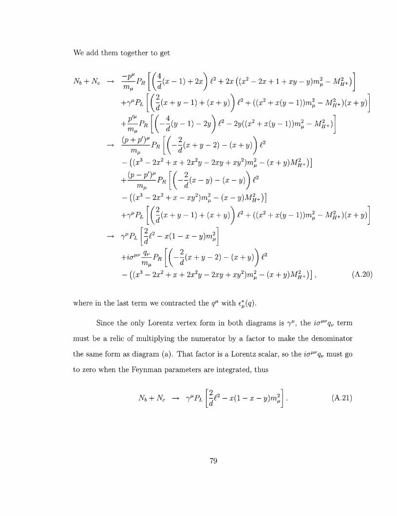
We add them together to get

Nb + Nc -p»

Pi R

+YPL

+—PR

{P + p'Y

<f -(x - 1) + 2z W2 + 2rr ((x2 -2x + l + xy- y)m? - M^+)

cP 2 J I # 2 -(x + y-l) + {x + y))£2 + ((x2 + x(y - l))m2 - M2

H+){x + y)

<P — iy -l)-2y)£2- 2y((x2 + x(y - l))mj - M2

H+)

PR d

(x + y-2)-(x + y))£

- ((x3 -2x2 + x + 2x2y - 2xy + xy2)m\ - (x + y)M2H+)]

(P-P'Y P m„

R d (x-y)-(x-y)) £'

((x3 - 2x2 + x - xy2)m\ - (x - y)M2H+)]

(x + y-l) + (x + y))£2 + ((x2 + x(y - l))m2u - M2

H+)(x + y) +-fPi

I^PL

d

d £2 - x(l - x - y)m2

il

+ia^^PR m^ d

{x + y-2)-(x + y))£

((x3 -2x2 + x + 2x2y - 2xy + xy2)m\ - (x + y)M2H+)] , (A.20)

where in the last term we contracted the q11 with e*(g).

Since the only Lorentz vertex form in both diagrams is 7^, the iatJ,l/qu term

must be a relic of multiplying the numerator by a factor to make the denominator

the same form as diagram (a). That factor is a Lorentz scalar, so the ia^q^ must go

to zero when the Feynman parameters are integrated, thus

Nb + Nc rpL -£2 -x{l-x- y)ml d

(A.21)

79

Adding this to the numerator of diagram (a), the 7^ piece cancels, leaving

AT = Na + Nb + Nc

= [xm^l-x-y^ia^q.PR, (A.22)

which gives us a total amplitude of

iM = %^<K^f^ldxf^ dy z*M)us'(p') K ( l -x-y)} ia^quPRus(p)

(A.23) (£2 - A + ief

Because our remaining integral is finite, we have taken d —> 4.

We thus need to figure out how to do integrals of the form J -44^ ,£2_^ x3 .

When we encounter integrals over 3-vectors with integrands that are only in terms of

the magnitude, we use the trick of imagining the various ways the three components

can add up to a specific magnitude as the surface area of a 3-dimensional sphere with

radius the particular magnitude. Then we can simply integrate over the magnitude

and multiply by the appropriate weight factor for each magnitude, the surface area

of a sphere of radius that magnitude. In this case, we are dealing with 4-vectors, so

we would like to use a similar technique, but instead with a 4-dimensional sphere.

However, these vector are not euclidean vectors, where e2 = e\ + e\ + e\ + e|, but are

instead Lorentz vectors with the relationship £2 = £\ — £\ — £\ — £2. To rectify this,

we define a euclidean 4-vector e such that

e0 = i£0 , e~£. (A.24)

80

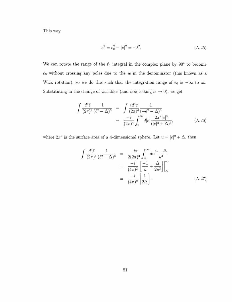
This way,

e2 = e2 + \e\2 = -£2 (A.25)

We can rotate the range of the £0 integral in the complex plane by 90° to become

e0 without crossing any poles due to the ie in the denominator (this known as a

Wick rotation), so we do this such that the integration range of e0 is — oo to oo.

Substituting in the change of variables (and now letting ie —> 0), we get

d4£ (2TT)4 (£2 - A)3

id4 id e

(2

(2TT)4 ( -e2 - A)3

-i f°° „ , 27r2|e|3

wi dle] (|e|2 + A)3 '

(A.26)

where 2-7T2 is the surface area of a 4-dimensional sphere. Let u = \e\2 + A, then

dA£ -ITT

(2TT)4 (£2 - A)3 2(2TT)3

—i

—i

du u A

- 1

•u°

_ A_ u 2u2

' 1 1 2A "

(A.27)

81

Thus integrating over £ in our amplitude we get

iM %z2<uUu* l rl-x

f dx f Jo Jo

dy (4TT)5 2A

-l-x

xe;(q)us (p')Nus(p)

%^zZ<u^j0dxSo dy

^(q)us'(p') [xm^l -x-y)] ia^qvPRus{p) x

2e -i (x + y)M2

H+

= (4 2 E<^e^<(?)^)^ V^>)

f dx f Jo Jo

X

2e - i v\ (4TT)2

^ ( 1 - X - J , )

a;+ 2/

7. # +

(A.28)

This is in agreement with the general result given in Eq. 7 of Ref. [27].

Next we calculate the amplitude squared averaged over initial spins and

82

summed over final spins and polarizations:

lZ\Mf - i £ ss'pol ss'pol

-i e m M Q(^)2v2M2

H H+ zZ<u^u-

xus(p)PLia^qaus\p')ep(q)e;(q)us'(p')ia^q„PRus(p)

2 I I 2

1 f 1 e m ^ \ k-^ 2TJ*TJ

2\6(4n)2v2M2HJ | 2 L m ^ ^ ^ |

xTr [{f + mli)PLi<r°pq(,ty' + me){-gp^)ia^qvPR}

1 / 1 e m„ z2<u*^ 8 V6(4TT)2 v2 M2

H+.

xTr [Q* + mM)PL(7/,7<J - I'lM'W + ™e)(7V ~ TY)Q»PR

_1 ( 1 e mM

8 V6(4vr)2^22M^+.

xpap'pq^Tv [r(wa ~ -Y'l^iY-f ~ YY)PR]

1 / 1 em.

E < ^

8 V6(47r)2i;2M£+ E < ^

x - 8 m *

e2 ml

36(4TT)4 v4 M4

«•+ E<^« (A

The rest of the calculation is illustrated in Sec. 4.4.

83

References

[i]

[2]

[3

K

[5

S. M. Davidson and H. E. Logan, Phys. Rev. D 80, 095008 (2009).

S.M. Davidson and H.E. Logan, in preparation

S. Willenbrock, arXiv:hep-ph/0410370.

A. Zee, Quantum Field Theory in a Nutshell, Princeton University Press (2003).

C. Amsler et al. (Particle Data Group), Phys. Lett. B 667, 1 (2008).

R. Davis, Prog. Part. Nucl. Phys. 32, 13 (1994).

Z. Maki, M. Nakagawa and S. Sakata, Prog. Theor. Phys. 28, 870 (1962).

[8] Y. Fukuda et al. [Super-Kamiokande Collaboration], Phys. Rev. Lett. 81, 1562

(1998) [arXiv:hep-ex/9807003].

[9] B. Aharmim et al. [SNO Collaboration], Phys. Rev. Lett. 101, 111301 (2008)

[arXiv: 0806.0989 [nucl-ex]].

[10] L. Wolfenstein, Phys. Rev. D 17, 2369 (1978); S. Mikheyev and A. Smirnov, in

Proceedings of the Tenth International Workshop on Weak Interactions, Savon-

lina, Finland, June, 1985.

84

[11] CHOOZ Collaboration, M. Apollonio et al, Phys. Lett. B 466, 415 (1999); Eur.

Phys. J. C 27, 331 (2003).

[12] K2K Collaboration, M.H. Ahn et ai, Phys. Rev. Lett. 90, 041801 (2003).

[13] G.L. Fogli, E. Lisi, A. Marrone and A. Palazzo, Prog. Part. Nucl. Phys. 57, 742

(2006).

[14] Lawrence Berkeley National Lab (URL: http://www.lbl.gov/Publications/YOS/Mar/

neutrinos-2 .html)

[15] E. Ma, Phys. Rev. Lett. 86, 2502 (2001).

[16] S. Gabriel and S. Nandi, Phys. Lett. B 655, 141 (2007).

[17] T. Fukuyama and K. Tsumura, arXiv:0809.5221 [hep-ph].

[18] P. Fileviez Perez, T. Han, G. y. Huang, T. Li and K. Wang, Phys. Rev. D 78,

015018 (2008) [arXiv:0805.3536 [hep-ph]].

[19] K. A. Olive, G. Steigman, and T. P. Walker, Phys.Rept. 333, 389-407 (2000).

[20] E. W. Kolb and M. S. Turner, The Early Universe, San Juan: Addison-Wesley,

1990.

[21] G. Steigman, K. A. Olive and D. N. Schramm, Phys. Rev. Lett. 43, 239 (1979).

[22] A. Goobar, S. Hannestad, E. Mortsell and H. Tu, JCAP 0606, 019 (2006)

[arXiv:astro-ph/0602155].

[23] J. Michael Roney, Nuclear Physics B (Proc. Suppl.) 169, 379386 (2007).

85

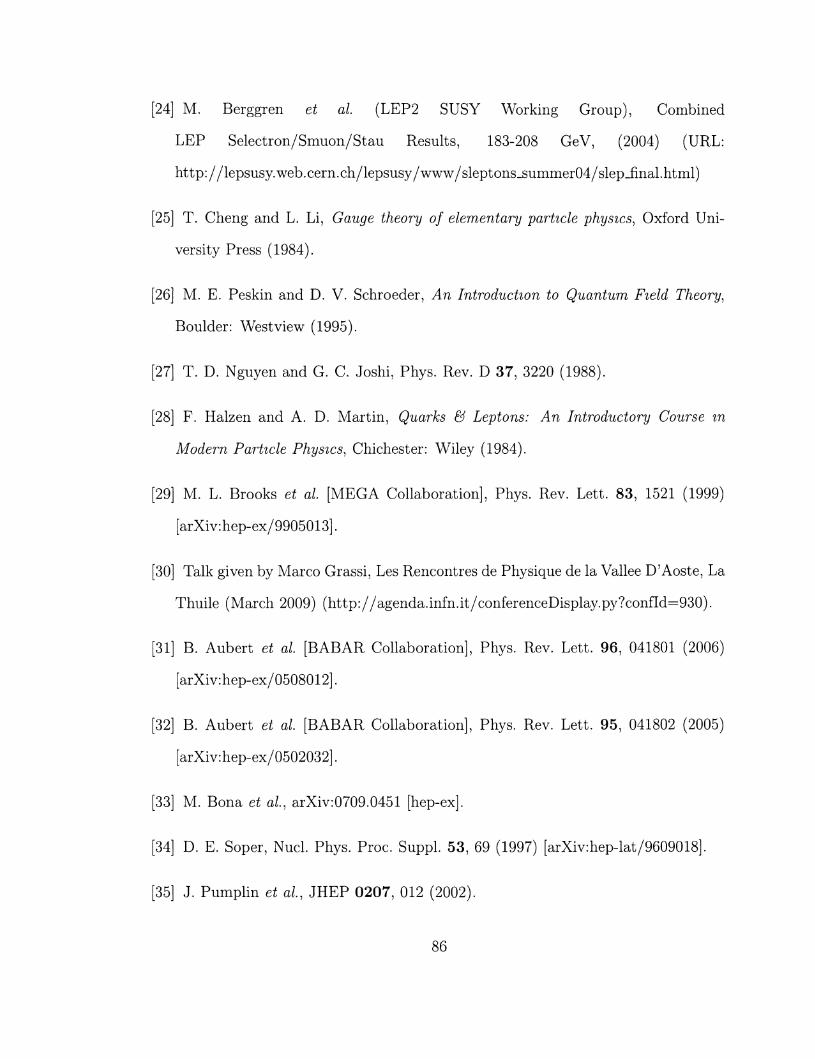
[24] M. Berggren et al. (LEP2 SUSY Working Group), Combined

LEP Selectron/Smuon/Stau Results, 183-208 GeV, (2004) (URL:

http://lepsusy.web.cern.ch/lepsusy/www/sleptons_summer04/slepJinal.html)

[25] T. Cheng and L. Li, Gauge theory of elementary particle physics, Oxford Uni­

versity Press (1984).

[26] M. E. Peskin and D. V. Schroeder, An Introduction to Quantum Field Theory,

Boulder: Westview (1995).

[27] T. D. Nguyen and G. C. Joshi, Phys. Rev. D 37, 3220 (1988).

[28] F. Halzen and A. D. Martin, Quarks & Leptons: An Introductory Course in

Modern Particle Physics, Chichester: Wiley (1984).

[29] M. L. Brooks et al [MEGA Collaboration], Phys. Rev. Lett. 83, 1521 (1999)

[arXiv:hep-ex/9905013].

[30] Talk given by Marco Grassi, Les Rencontres de Physique de la Vallee D'Aoste, La

Thuile (March 2009) (http://agenda.infn.it/conferenceDisplay.py?confId=930).

[31] B. Aubert et al. [BABAR Collaboration], Phys. Rev. Lett. 96, 041801 (2006)

[arXiv:hep-ex/0508012].

[32] B. Aubert et al. [BABAR Collaboration], Phys. Rev. Lett. 95, 041802 (2005)

[arXiv:hep-ex/0502032].

[33] M. Bona et al, arXiv:0709.0451 [hep-ex].

[34] D. E. Soper, Nucl. Phys. Proc. Suppl. 53, 69 (1997) [arXiv:hep-lat/9609018].

[35] J. Pumplin et al, JHEP 0207, 012 (2002).

86

[36

[37

[38

[39

[40;

[41

[42

[43;

[44;

[45;

W. Beenakker et al, Phys. Rev. Lett. 83, 3780 (1999).

A. Alves and T. Plehn, Phys. Rev. D 71, 115014 (2005) [arXiv:hep-ph/0503135].

H. Baer, B. W. Harris and M. H. Reno, Phys. Rev. D 57, 5871 (1998) [arXiv:hep-

ph/9712315].

J. Alwall et al, JHEP 0709, 028 (2007).

T. Stelzer and W. F. Long, Comput. Phys. Commun. 81, 357 (1994) [arXiv:hep-

ph/9401258].

F. Maltoni and T. Stelzer, JHEP 0302, 027 (2003) [arXiv:hep-ph/0208156].

T. Sjostrand, S. Mrenna and P. Z. Skands, JHEP 0605, 026 (2006) [arXiv:hep-

ph/0603175].

J. Conway et al, available from http://www.physics.ucdavis.edu/~conway/

research/software/pgs/pgs4-general .htm

J. M. Campbell and R. K. Ellis, Phys. Rev. D 60, 113006 (1999).

R. Bonciani, S. Catani, M. L. Mangano and P. Nason, Nucl. Phys. B 529, 424

(1998).

87