ph.d. thesis by kamran khan
TRANSCRIPT

ECOLOGICAL AND SOCIO-ECONOMIC IMPACTS OF
MONOCULTURE OF EXOTIC TREE SPECIES IN
DISTRICT MALAKAND, PAKISTAN
Ph.D. THESIS
BY
KAMRAN KHAN
CENTRE OF PLANT BIODIVERSITY
UNIVERSITY OF PESHAWAR
Session 2015-2016

ECOLOGICAL AND SOCIO-ECONOMIC IMPACTS OF
MONOCULTURE OF EXOTIC TREE SPECIES IN DISTRICT
MALAKAND, PAKISTAN
A thesis submitted to the Centre of Plant Biodiversity, University of Peshawar in
partial fulfilment of the requirement for the degree of
DOCTOR OF PHILOSOPHY
IN
PLANT BIODIVERSITY AND CONSERVATION
BY
KAMRAN KHAN
RESEARCH SUPERVISOR: DR. ASAD ULLAH
Graduate Studies Committee:
1. Dr. Asad Ullah Convener
2. Prof. Dr. Sardar Khan Member
3. Dr. Zahir Muhammad Member
4. Dr. Sana Ullah Khan Member
5. Dr. Syed Ghias Ali Member
CENTER OF PLANT BIODIVERSITY
UNIVERSITY OF PESHAWAR
SESSION 2015-2016


PUBLICATION OPTION
All rights of publication are hereby reserved by the scholar, including right to reproduce
this thesis in any form for a period of 5 years from the date of submission.
Kamran Khan


Dedication
Dedicated to my Parents
and Teachers

Landcover Map of Malakand Protected area
Source: Forest Management Centre, Khyber Pukhtunkhwa Environment
Department, Pakistan.

VITAE
Born on 1st January 1987 in Thana Malakand, Khyber Pakhtunkhwa, Pakistan.
BS (Hons.) in Forestry from University of Malakand in 2010.
M.Phil. in Plant Biodiversity and Conservation from University of Peshawar in 2016.
Presently working as Range Forest Officer at Pakistan Forest Institute Peshawar.
Major Field of Study
Plant Biodiversity and Conservation
S. No Course No Title of course Tutor name
1 CPB-801 Plant Systematics (Theory) Dr. Asad Ullah
2 CPB-801 Plant Systematics (Lab.) Dr. Asad Ullah
3 CPB-806 Plant Reproductive Biology
(Theory)
Dr. Syed Ghias Ali
4 CPB-806 Plant Reproductive Biology
(Lab.)
Dr. Syed Ghias Ali
5 CPB-809 Phylogenetics of Vascular
Plants (Theory)
Dr. Asad Ullah
6 CPB-809 Phylogenetics of Vascular
Plants (Lab.)
Dr. Asad Ullah
7 CPB-811 Soil Plant Relationship
(Theory)
Dr. Fazal Hadi
8 CPB-813 Research Methodology
(Theory)
Dr. Syed Ghias Ali

TABLE OF CONTENTS
S. No. Title Page No.
Acknowledgements i
Abstract iii
1 CHAPTER 1: INTRODUCTION 1
1.1 Description of the study area 1
1.1.2 Area location and boundaries 1
1.1.3 Soil and geology 1
1.1.4 Flora and fauna 1
1.1.5 Climate 2
1.1.6 Socio-economic activities 2
1.2 Topic introduction 3
1.3 Problem statement 4
1.4 Aim and objectives 6
1.5 Justification of study 6
1.6 Socioeconomic benefits 6
2 CHAPTER 2: REVIEW OF LITERATURE 7
3 CHAPTER 3: MATERIALS AND METHODS 31
3.1 Selection of research plots 31
3.2 Data collection 32
3.3 Assessment of ecological impacts 33
A) Study on undergrowth vegetation 33
Undergrowth vegetation survey 33
Determination of quadrat size 33
Quadrat sampling and recording 33
Specimen collection and preservation 34
Specimen examination 34
Specimen identification and nomenclatural Information 35
Supplementary data collection 35
Data analysis 35

Shannon-Wiener Diversity Index 38
B) Study on soil physico-chemical properties 38
Soil sample collection 38
Soil data analysis 39
3.4 Socio-economic impacts of monoculture of exotic tree species 41
Selection and investigation of woodlots and tree growers 41
Benefit cost analysis on the woodlots plantations of exotic tree
species
42
Focus group discussion 43
Key informant interview 44
Secondary data collection 45
3.5 Discharge rate and water table measurement 45
4 CHAPTER 4: RESULTS AND DISCUSSIONS 46
4.1 Ecological impacts 47
4.1.1 Undergrowth vegetation 47
4.1.2 Floristic composition and taxonomic diversity 47
4.1.3 Phytosociology of undergrowth vegetation 56
Undergrowth plant density 56
Relative density 58
Frequency 60
Relative frequency 60
Abundance 61
Relative abundance 62
Communities structure 63
4.1.4 Phytodiversity index 64
4.1.5 Tree productivity 66
4.2 Soil physico-chemical properties 68
pH 68
Organic matter (OM) 70
Organic Carbon (OC) 73
Soil Electric conductivity (EC) 74
Nitrogen (N) 76

Phosphorus (P) 78
Potassium (K) 80
Calcium Carbonate (CaCO3) 81
4.3. Socio-economic impacts of the monoculture of exotic tree species 83
4.3.1 Basic information of the tree growers 83
Education 84
Occupation 84
Land use pattern 84
4.3.2 Characteristics and factors of woodlot plantation of exotic tree
species
87
4.3.3 Expenditure for woodlot plantation of exotic tree species 90
4.3.4 Benefit cost analysis on woodlots of exotic tree species 93
Net Present Value, Internal Rate of Return and Benefit Cost Ratio 93
Sensitivity analysis 93
Plantation damaging factors 96
Purpose of growing exotic species 96
4.3.5 Sources of energy for fulfilling domestic/commercial needs of
people
97
4.3.6 Species used for fuelwood, rates/mound and sale in the market 98
4.3.7 Relative merits and demerits of selected exotic and indigenous
tree species
98
4.4 Impact of exotic plantations on ground water 99
4.4.1 Impact of exotic plantations on springs 100
4.4.2 Impact of exotic plantations on discharge rate of springs 101
5 CHAPTER 5: CONCLUSIONS AND
RECOMMENDATIONS
103
5.1 Conclusions 103
5.2 Recommendations 103
References 105
Appendices 120
Plagiarism certificate 226

LIST OF TABLES
Table No. Title Page No.
Table-4.1 Shannon-Wiener diversity index values recorded for different
research plots.
65
Table-4.2 Mean values of Shannon- weiver diversity index of different
research plots calculated after analysis using statistics 8.1
software two-way ANOVA (LSD) was used to test for significant
differences (P<0.05) for marginal means of variables.
66
Table-4.3 Density of trees, height, DBH, basal area and gross tree stem
volume in different plots of exotic and indigenous species.
67
Table-4.4 Mean values of different physico-chemical parameters of soil of
different research plots.
68
Table-4.5 Means showing nutritional status of different species plots. 76
Table-4.6 Basic information of woodlot tree grower of District Malakand. 85
Table-4.7 Characteristics of different woodlot plantation raised by the tree
growers in District Malaakand.
88
Table-4.8 Expenditure of tree growers for raising one-hectare woodlot
plantations in District Malakand.
91
Table-4.9 Sensitivity of BCR and NPV with reference to changes in the
interest rate for one hectare woodlot monoculture plantation in
District Malakand.
93
Table-4.10 Future valuation and expected profit of woodlot trees per hectare
raised in District Malakand.
94
Table-4.11 Rate per mound of different species and their sale in the local
market
98
Table-4.12 Depth of water table before and after exotic plantation 99
Table-4.13 Number of springs before and after exotic plantations 100
Table-4.14 Discharge rate of springs before and after exotic plantations 101

LIST OF FIGURES
Figure No. Title Page No.
Fig. 4.1 Taxonomic diversity of flora of all research plots. 48
Fig. 4.2 Taxonomic diversity of flora of indigenous research plots. 49
Fig. 4.3 Taxonomic diversity of flora of exotic research plots. 49
Fig. 4.4 Morphological diversity of plants species of all plots. 51
Fig. 4.5 Morphological diversity of plants species of indigenous plots. 52
Fig. 4.6 Morphological diversity of plants species of exotic plots. 52
Fig. 4.7 Numbers of annuals, perennials and biennials in all research plots. 53
Fig. 4.8 Numbers of annuals, perennials and biennials in indigenous plots. 53
Fig. 4.9 Numbers of annuals, perennials and biennials in exotic plots. 54
Fig. 4.10 Species composition in different tree plots in spring, monsoon and
winter seasons in Malakand area.
54
Fig. 4.11 Number of all undergrowth plants and number of tree species in
exotic and indigenous research plots.
55
Fig. 4.12 Number of undergrowth tree species found in different research
plots in the research area.
56
Fig. 4.13 Undergrowth densities per hectare considering all undergrowth
species in three seasons in different research plots in the study area.
58
Fig. 4.14 Average undergrowth density per hectare considering all
undergrowth species in different tree plots in research area.
58
Fig. 4.15 Showing soil pH of plots of different plants in different seasons. 69
Fig. 4.16 Showing organic matter (%) in plots of different plants in
different seasons.
71
Fig. 4.17 Showing soil organic Carbon (%) in plots of different plants in
different seasons.
73
Fig. 4.18 Showing soil electrical conductivity of plots of different plants in
different seasons.
75
Fig. 4.19 Showing Soil total Nitrogen in percent of plots of different plants
in different seasons.
76
Fig. 4.20 Showing soil available Phosphorus (ppm) of plots of different
plants in different seasons.
78
Fig. 4.21 Showing soil Potassium (ppm) of different plants in different
seasons.
80
Fig. 4.22 Showing Calcium Carbonate (mmole /meter) of plots of different
plants in different seasons.
82
Fig. 4.23 Tree grower perception (%age) on plantation damaging factors. 96
Fig. 4.24 Sources of energy used for fulfilling domestic/commercial needs
of the people.
97

LIST OF APPENDICES
S. No. Title Page
No.
Appendix-1 Checklist of undergrowth plant species recorded from
research plots at Malakand.
120
Appendix-2 Total no. of individuals, Density, Relative density, frequency,
relative frequency, abundance, relative abundance considering
all undergrowth species in indigenous plots.
127
Appendix-3 Total no. of individuals, Density, Relative density, frequency,
relative frequency, abundance, relative abundance considering
all undergrowth species in exotic plots.
133
Appendix-4 Total no. of individuals, Density, Relative density, frequency,
relative frequency, abundance, relative abundance considering
only tree undergrowth species in indigenous plots.
137
Appendix-5 Total no. of individuals, Density, Relative density, frequency,
relative frequency, abundance, relative abundance considering
only tree undergrowth species in exotic plots.
138
Appendix-6.1 Shannon-Wiener diversity index (H) values considering all
undergrowth plant species recorded from Pinus roxburghii
plots during spring season
139
Appendix-6.2 Shannon-Wiener diversity index (H) values considering all
undergrowth plant species recorded from Pinus roxburghii
plots during monsoon season.
142
Appendix-6.3 Shannon-Wiener diversity index (H) values considering all
undergrowth plant species recorded from Pinus roxburghii
plots during winter season.
145
Appendix-6.4 Shannon-Wiener diversity index (H) values considering
undergrowth tree species only recorded from Pinus roxburghii
plots during summer season.
148
Appendix-6.5 Shannon-Wiener diversity index (H) values considering
undergrowth tree species only recorded from Pinus roxburghii
plots during winter season.
149
Appendix-6.6 Shannon-Wiener diversity index (H) values considering
undergrowth tree species only recorded from Pinus roxburghii
plots during winter season.
150
Appendix-6.7 Shannon-Wiener diversity index (H) values considering all
undergrowth plant species recorded from E. camaldulensis
plots during spring season
151
Appendix-6.8 Shannon-Wiener diversity index (H) values considering all
undergrowth plant species recorded from E. camaldulensis
plots during monsoon season.
153
Appendix-6.9 Shannon-Wiener diversity index (H) values considering all
undergrowth plant species recorded from E. camaldulensis
plots during winter season.
155
Appendix-6.10 Shannon-Wiener diversity index (H) values considering
undergrowth tree species only recorded from E. camaldulensis
plots during spring season
157

Appendix-6.11 Shannon-Wiener diversity index (H) values considering
undergrowth tree species only recorded from E. camaldulensis
plots during monsoon season
158
Appendix-6.12 Shannon-Wiener diversity index (H) values considering
undergrowth tree species only recorded from E. camaldulensis
plots during winter season.
159
Appendix-6.13 Shannon-Wiener diversity index (H) values considering all
undergrowth plant species recorded from Acacia modesta
plots during spring season.
160
Appendix-6.14 Shannon-Wiener diversity index (H) values considering all
undergrowth plant species recorded from Acacia modesta
plots during monsoon season.
163
Appendix-6.15 Shannon-Wiener diversity index (H) values considering all
undergrowth plant species recorded from Acacia modesta
plots during winter season.
166
Appendix-6.16 Shannon-Wiener diversity index (H) values considering
undergrowth tree species only recorded from Acacia modesta
plots during spring season.
169
Appendix-6.17 Shannon-Wiener diversity index (H) values considering
undergrowth tree species only recorded from Acacia modesta
plots during monsoon season.
170
Appendix-6.18 Shannon-Wiener diversity index (H) values considering
undergrowth tree species only recorded from Acacia modesta
plots during winter season.
171
Appendix-6.19 Shannon-Wiener diversity index (H) value considering all
undergrowth plant species recorded from R. pseudoacacia
plots during spring season.
172
Appendix-6.20 Shannon-Wiener diversity index (H) value considering all
undergrowth plant species recorded from R. pseudoacacia
plots during monsoon season.
174
Appendix-6.21 Shannon-Wiener diversity index (H) value considering all
undergrowth plant species recorded from R. pseudoacacia
plots during winter season
176
Appendix-6.22 Shannon-Wiener diversity index (H) values considering
undergrowth tree species only recorded from R. pseudoacacia
plots during spring season.
178
Appendix-6.23 Shannon-Wiener diversity index (H) values considering
undergrowth tree species only recorded from R. pseudoacacia
plots during monsoon season.
179
Appendix-6.24 Shannon-Wiener diversity index (H) values considering
undergrowth tree species only recorded from R. pseudoacacia
plots during winter season.
180
Appendix-6.25 Anova results for comparison of SWDI (H) values of all
research plots considering all undergrowth.
181
Appendix-6.26 Anova results for comparison of SWDI (H) values of all
research plots considering only trees species as undergrowth.
182
Appendix-6.27 Anova results for comparison of SWDI (H) values B/w exotic
and indigenous research plots considering all undergrowth.
183

Appendix-6.28 Anova results for comparison of SWDI (H) values B/w exotic
and indigenous research plots considering only tree species as
undergrowth.
184
Appendix-7.1 Different soil parameters recorded from exotic and indigenous
tree plots during winter season 2017.
185
Appendix-7.2 Different soil parameters recorded from exotic and indigenous
tree plots during spring season 2018.
187
Appendix-7.3 Different soil parameters recorded from exotic and indigenous
tree plots during monsoon season 2018.
189
Appendix-8 Soil pH 191
Appendix-9 Organic Matter (OM) 194
Appendix-10 Organic carbon (OC) 197
Appendix-11 Electric conductivity (EC) 200
Appendix-12 Total Nitrogen (N) 203
Appendix-13 Phosphorus (P) 206
Appendix-14 Potassium (K) 209
Appendix-15 Calcium Carbonate (CaCO3) 212
Appendix-16 Calculation of Internal Rate of Return (IRR) 215
Appendix-17 Calculation of Net present value (NPV) and Benefit cost Ratio
(BCR)
216
Appendix-18 Average benefit cost analysis for one-hectare woodlot
plantations in District Malakand
217
Appendix-19 Questionnaire 218
Appendix-20 Photographic Presentation 220

LIST OF MAP
S. No. Map Title Page No.
1 Map of the research plots located at District Malakand 31

i
ACKNOWLEDGEMENTS
First of all, thanks to ALLAH Almighty, the most merciful and beneficient enabling me
to complete this task. Darood-Wa-Salam on his Prophet Muhammad (PBUH), the
source of knowledge and wisdom for the entire humanity.
Its my great pleasure to express my heartiest gratitude, most sincere appreciation and
profound thanks to my supervisors Dr. Asad Ullah, Director Centre of Plant
Biodiversity, University of Peshawar, Khyber Pukhtunkhwa, Pakistan for his overall
supervision, fruitful criticism, valuable suggestions, proper evaluation and continuous
encouragement throughout the research period.
My sincere appreciation goes to all honorable inland and foreign members of the thesis
evaluation committee for their critical and constructive comments and suggestions on
all aspects of the dissertation. I gracefully acknowledge the valuable comments, critics
and suggestions made by Prof. Jerry Roberts, Deputy Vice Chancellor Research and
Enterprise, University of Plymouth, UK for overall improvement of this research work.
I am highly grateful to Dr. Syed Ghias Ali, Dr. Syed Mukaram Shah and all the teaching
and supporting staff of Centre of Plant Biodiversity, University of Peshawar for their
encouragement and support throughout my study period.
I am also thankful to Prof. Dr. Zafar Iqbal, Meritorious Professor, Dean Faculty of Life
and Environmental Sciences, Prof. Dr. Bashir Ahmad, Ex-Dean Faculty of Life and
Environmental Sciences for his valuable suggestions in the research proposal, Prof. Dr.
Siraj-Ud-Din, Dr. Zahir Muhammad, Department of Botany, Prof. Dr. Akram Shah,
Department of Zoology and Prof. Dr. Sardar Khan, Department of Environmental
Sciences, University of Peshawar for their valuable suggestions and corrections in the
research proposal and dissertation throughout the entire study period.
I am especially grateful to Mr. Ghulam Jelani, Lecturer, Department of Botany
University of Peshawar, for his help in identification of plants.
My sincere gratitude goes to Mr. Yousuf Noor, Senior Research Officer, Dr. Samad,
Research Officer and staff of Agriculture Research Institute at Tarnab Farm, Peshawar
for providing permission and laboratory facilities for soil analysis. I must thank to Khan

ii
Afzal, Laboratory Attendant and Staff of Agriculture Research Institute at Tarnab Farm,
Peshawar for providing support and facilities for soil analytical work and also for their
help and suggestions. Thanks are also due to Professor Dr. Farman Ullah, Soil and
Environment Department, The University of Agriculture, Peshawar and Mr. Mukhtiar
Ahmad, M.Phil. Scholar, Soil and Environment Department, The University of
Agriculture, Peshawar for helping in the soil data analysis. I am also thankful to Dr.
Syed Ghias Ali, Assistant Professor, Centre of Plant Biodiversity for helping and
guiding me in proper statistical interpretation of the results.
I am also highly thankful to the field staff of Khyber Pakhtunkhwa Forest Department,
Malakand Forest Division, Malakand for helping me in the data collection during field
survey from the research area throughout the study period. My sincere gratitude to the
forest villagers, local peoples of the study area who consented to provide information
without which it would not be possible to conduct this research work.
Last but not the least, I am extremely grateful to my beloved parents, brothers, sisters,
friends and other relatives for their continuous moral support and encouragement.
Kamran Khan
iii
Ecological and Socio-economic Impacts of Monoculture of Exotic Tree Species in
District Malakand, Pakistan
Abstract
This study was carried out to investigate the impacts of monoculture of exotic
tree species (Eucalyptus camaldulensis and Robinia pseudoacacia) on species
composition and diversity of the undergrowths, physico-chemical properties of soil,
ground water and the socio-economy of the local people in relation to indigenous (Pinus
roxburghii and Acacia modesta) tree plots in district Malakand. Data was collected
from 12 research plots of exotic and indigenous tree species located in public and
private land, and 30 woodlots of exotic tree species through intensive field visits
conducted from April 2017 to March 2019.
A total of 174 plants species which belongs to 74 families and 150 genera were
reported in the selected research plots of trees of indigenous (Pinus roxburghii and
Acacia modesta) and exotic (Eucalyptus camaldulensis and Robinia pseudoacacia)
species. Among the recorded species 143 (82%) were dicotyledons, 26 (15%) species
were monocotyledons and 4 (2.3%) were pteridophytes while only 1 (0.7%) of the
plants recorded were gymnosperms. In both exotic and indigenous tree stands, 97% of
the plant species were Angiosperms, 2.3% were Pteridophytes and only 0.7% were
Gymnosperms. A total of 149 undergrowth species including 23 tree species were found
in indigenous stand and 111 species including 18 tree species in exotic stands. The
exotic tree plots comprised 22% less species in comparison to indigenous plots.
In spring, monsoon and winter seasons, 83 species each in spring and monsoon
and 62 undergrowth species were found in winter season in Pinus roxburghii plots. In
Acacia, Eucalyptus and Robinia plots a total of 89,70 and 67 species respectively were
found in each spring and monsoon season while 67,58 and 34 species respectively in
winter season.
In indigenous tree plots, Acacia modesta was found to have the highest relative
density whereas in exotic plots Robinia pseudoacacia was most prevalent. The shrub
species Dodonaea viscosa was found to have the highest relative frequency in both
exotic and indigenous tree plots respectively.

iv
The average value of Shannon-Wiener diversity index was 3.41 and 3.73
collectively in all exotic and indigenous plots respectively, which depict that the extent
of species diversity was higher in indigenous tree plots than in exotic tree plots. Out of
the four categories of sampling research plots, the Pinus roxburghii plots were clearly
rich in species diversity.
Result showed that soil properties were significantly different in indigenous and
exotic research plots. Soil OM, OC, pH, N, P, K and Calcium Carbonate of the soil of
Acacia modesta plots, Pinus roxburghii plots, Robinia pseudoacacia plots and
Eucalyptus camaldulensis plots were significantly different. Findings of these results
showed that, soil in the exotic species plots of Robinia pseudoacacia and Eucalyptus
camaldulensis were less fertile as compared to the soil in the indigenous plots of Acacia
modesta plots and Pinus roxburghii.
The two major reasons for plantations of fast growing Eucalyptus camaldulensis
over other species for woodlot plantation by the local people were the production of
fuel wood and early income generation from their sale. On average, a tree grower
spends Rs. 159144 for raising one-hectare woodlot plot, and is expecting to sell the
timber for Rs. 2049478 ha after completion of tree rotation, whereas the expected net
profit from timber sale was Rs. 1956206 per ha. Benefit cost analysis for one-hectare
private woodlot plantations showed that, the BCR was 1.25 on ±10 years’ rotation
which was comparatively higher and the NPV was Rs. 165982, whereas the IRR was
14.33% found to be comparatively higher. The base case scenario (lending interest rate)
in interest rate 10% showed the BCR 1.25 and NPV Rs. 165982, which was profitable
in plantation business. If the less interest rate trend found in future (government lending
interest rate decreasing) that will confirm more BCR and NPV, which indicated better
profit for tree growers. The benefit cost analysis indicated that the woodlot project was
financially viable.
Local peoples were found to be interested in planting fast growing exotic tree
species to meet their immediate financial demand within a short period. The
monoculture of exotic species seems financially profitable for the short term projects
and to have a promising prospect in district malakand and its adjacent areas, but if the
long term perspectives are considered then ultimately it is not economically viable and
not appropriate to ensure the sustainability of biodiversity and ecosystem conservation.

v
During the questionnaire survey, the villagers and tree growers identified some
problems with the exotic species, such as the trees of exotic species absorb more ground
water and that other trees hardly grow under them; they had a low number of twigs and
leaves that not decompose after falling on the ground; they allow minimum collection
of fuel wood; and growth of crops is slow under the exotic trees etc. They also opined
that, it was not meaningful to replace Acacia modesta and Pinus roxburghii trees by
any exotic species. Monoculture of exotic species should, therefore, be discouraged for
afforestation but might be operational in some degraded, barren or specified lands.

1
CHAPTER-1
INTRODUCTION
1.1 DESCRIPTION OF THE STUDY AREA
The location, soil, climate, floristic composition and socio-economic aspects of
the study area of District Malakand have been described below.
1.1.2 AREA LOCATION AND BOUNDARIES
The total area of District Malakand is 952 km2. It lies on 34°22՜ to 35°43՜ N
latitudes and 71°36՜ to 72°12՜ E longitudes. The elevation of the study area ranges from
600 to 850 meters. It is surrounded by a series of mountains on the North East which
separate it from District Swat and other ranges of mountains to the west separate it from
Bajaur and Mohmand Agencies. It is surrounded on the north by District Lower Dir, on
north west by District Bajuar, the District Buner lies on the East, the District Mardan is
situated on the south and Charsadda district and Mohmand agency on the south west
(GOP, 2017).
1.1.3 SOIL AND GEOLOGY
The soil composition of Malakand is sandy-loam with gravel layers/loam and
developed from old pediment materials. Soil of the area is either rain fed or irrigated.
The following rock types are present in the area. The northern part of the protected area
is occupied by the main mental thrust material also known as melange zone rocks.
Composed of voleaie, phyllites, shales, green schist, quartzite and other oceanic meta
sediments. The middle part of the agency comprised meta sediments and granite rocks.
The meta sediment is divided into four formations viz. Marghuzar formation. Rahsala
formation, Saidu formation and granitic formation. The granitic formations are further
divided to Malakand granite, Chakdara granite and Bazdara granite. The Malakand
power house Tunnel passes through these rocks formations. In the south near Dargai is
the ophite rock known as Dargai Ophiolite. These Ophiolite rocks contain chromate,
soapstone, asbestos manganese and magnesite. Further south up to Skhakot is the
alluvial plain area, where maximum population of the Malakand is living (GOP, 2017).
1.1.4 FLORA AND FAUNA
Malakand Scrub forest is dominated by native species of Acacia modesta, Pinus
roxburghii, Dodonea viscosa, Olea ferrugenia, Ziziphus mauratiana, Z. numularia,
Acacia nilotica, Punica granatum, Monotheca buxifolia, Capparis aphylla,

2
Cymbopogan jawarancusa, Cynodon dactylon, Cenchrus ciliaris and Chryspogan.
Commonly occurring animals in the area including jackal, leopard, monkey and
wolf. As a result of huge deforestation they became scarce.
1.1.5 CLIMATE
The study area has a dry sub-tropical climate. The rainfall is irregular, mostly
occurring in winter from December to March. It has a hot summer and cold winter. The
average rainfall is low which ranges from 600 to 650 mm (GOP, 2008) and therefore
soil requires artificial irrigation. The month of June is the hottest, having a mean
maximum temperature of 40 oC. The coldest months are December and January, with a
mean minimum temperature of 0 oC (GOP, 2013). Snowfall occurs much rarely and
sometime occurs on mountain tops, which melts rapidly. Frost occurs more commonly
and start by the mid November and its intensity is severe during December and January.
1.1.6 SOCIO-ECONOMIC ACTIVITIES
About 50% of the land area of Malakand Agency is cultivable while the
remaining consist of hills. The cultivable lands are mostly privately held. Nearly 63%
of the households are landless and rely upon labour to earn their livelihood. 32%
among the owners has landholding size less than hectare and 45% of them have
landholding size less than 4 hectares. Agriculture crops like sugarcane, rice wheat,
corn are major crops on irrigated lands. Major portion of the cultivated lands are also
used for growing fruit orchards like citrus, peach and guava. The people of the study
area are interested in raising fast growing tree species around their fruit orchards or on
the boundaries of their agriculture fields, such as Populus deltoides, Ailanthus
altissima and Eucalyptus species. They grow these trees for timber as well as fuel
wood production for their family consumption. About 40% of farmers depend on
agriculture for their livelihood.
The mountains are mostly owned by communities, and sometimes different
segments of the community. The area has protected forest in which the rights to collect
fuelwood and fodder exist. Therefore, most of the people have access to go and collect
the same from the forest which has created difficulties in management of the existing
forest area. The hillsides are mostly used by the local people for grazing livestock and
fuel wood collection. Some parts located at the west side of Malakand are severely
degraded and have very low production. The estimated forest cover is 7.2% of the area.

3
1.2 TOPIC INTRODUCTION
Pakistan forests cover an area of about 4.2 million ha i.e. 4.8% of the total land
area which is too low to fulfil the environmental and socio-economic needs of the
country when compared with the required 25% for the developing countries (GOP,
2005 and FAO, 2000). As a result of excessive rate of deforestation and degradation of
environment, Pakistan has limited forest resources having lowest proportions of area
under forest (Mcketta, 1990). Production from state owned forest are not enough to
meet the demand for timber and fuel wood, raw material for industries, energy
requirements of the agricultural sector and fodder for livestock (Sheikh, 1987),
dependency on conventional fuels like firewood (which alone accounts for 50% of rural
fuel needs), cow dung and agricultural residue indicates the importance of trees in
solving energy needs of rural communities (Siddiqui, 1997). To bridge the gap between
demand and supply of the forest produces, a number of tree plantation
projects/programs were launched by the Government and development agencies that
basically targeted the fallow land, marginal land, roadsides, railway, canal/river banks
and embankments (FAO/UNDP, 1981).
In Pakistan deliberate and planned attempts under the umbrella of social forestry
were made to improve the declining natural resources. For this purpose, many forestry
projects were launched. Most of these projects were donor financed while few were
NGO driven and even some were started by the local community themselves. The
Social Forestry Project in Malakand District was started in February, 1987 jointly by
Government of Pakistan and the Government of Netherland. The main objectives of
these plantations were to improve livelihood of the inhabitants by proper utilization of
hilly tracts and other useless land through increasing productivity. A total area of 28,078
hectares was planted with indigenous and fast growing exotic tree species in different
areas of Malakand, Dir and Alpuri. Among the planted exotic species Eucalyptus
camaldulensis, Robinia pseudoacacia, Ailanthus altisimma were predominant while
among the indigenous species Pinus roxburghii and Acacia modesta were dominant.
Some species among the exotics are causing a number of environmental and social
problems like low water table, micro climate change, soil erosion, fauna and flora loss
and dry springs (Hussain, 2002).
Generally exotic fast growing tree species are preferred in forestry plantation,
which contribute considerably to the economic growth of many regions. These
plantations not only produced extensive changes in natural ecosystem but also affect
4
ecosystem services and biodiversity, which can be mitigated by proper management
therefore, perpetuating this key economic sector (Richardson, 1998 and Hartley, 2002).
According to FAO (2010) natural forests of the world are decreasing day by day while
their fragmentation is increasing due to the expansion and replacement of these natural
forests by exotic tree plantation. Nowadays these plantations are most successful due
to high adoptability by farmers of developing countries. Such forest not only provide
shelter and decreasing edge effects but also enhance connectivity among existing forest
fragments and thus provide opportunities for eco tone specialists and potential forest
species to establish that may benefit from any other forest type (Christian et al., 1998;
Norton, 1998; Davis et al., 2001; Georgie et al., 2007; Richard et al., 2007 and Felton
et al., 2010). Despites such and several other beneficial uses, excessive monoculture
of exotic tree plantations are considered as a threat to existing biodiversity due to the
depletion of soil nutrients, pumping up of water resources, suppression of understory
vegetataion by secretion of allelopathic chemicals and ecosystem degradation (Carnus
et al., 2003; Evans, 1992; FAO, 2001; Proença et al., 2010; Pina, 1989; Jagger &
Pender, 2000; Temes et al., 1985 and Basanta et al., 1989). However, some studies
showed their potential for restoration of woody species diversity (Michelsen et al., 1996
and Yirdaw & Luukkanen, 2003).
Some public opinions have also been raised against the cultivation of exotic
species like Eucalyptus camaldulensis in plantation programs claiming that these
species have a damaging impact on the ecosystems. In this context, comparative studies
on the monoculture of exotic tree species versus indigenous tree species needed to be
conducted from ecological and socio-economic point of view for better understanding
required in correct choice and selection of tree species for future plantation programs
for sustainable development.
1.3 PROBLEM STATEMENT
Plantation in public and private land helps in improving the socioeconomic
condition of the rural people by generating income and employment but the
consequence or advantage and disadvantage of the plantation programs with exotic
species is a matter of great concern. Malakand is one of the districts where Forest
Department of Khyber Pakhtunkhwa province, NGOs, farmers and the local
community people raised large scale plantations of Eucalyptus camaldulensis and
Robinia pseudoacacia in their lands farms and cleared forest lands to get more

5
economic return within short time. Eucalyptus camaldulensis and Robinia
pseudoacacia are most commonly grown in Pakistan in various reforestation and
afforestation programs because of their fast growing characteristics and production of
high volumes of biomass within a short time, short rotation and ability to thrive in poor
soils.
With the increase in population of the study area, deforestation on large scale
took place, which reduced the vegetative cover and consequently, the forest is under
severe biotic pressure. To overcome this problem several attempts are made to carry
out plantation in the area. It has been observed that severe effects have been posed by
largescale plantations of exotic species resulting in to a number of environmental and
social problems like low water table, micro climate change, soil erosion, fauna and flora
loss and drying springs (Hussain, 2002). The native communities of plants were
reduced and were replaced by exotic plantations on large scale. It has also observed that
many species become endangered due to these exotics and the ecosystem services were
badly affected by such plants (Shinwari and Qaiser, 2011; Shinwari et al., 2012; Sangha
and Jalota, 2005; Gareca et al., 2007 and Wang et al., 2011). The extensive plantation
of exotics and its monoculture practices has resulted in to degradation of soil and
productivity due to amassing of allelo chemicals in soil (El-Khawas and Shehata, 2005
and Forrester et al., 2006).
Though, some studies on undergrowth species composition in different areas
have been carried out, However, no integrated and comparative study was carried out
on the composition of undergrowth and understory species diversity in exotic and
indigenous tree plantations. In this context, comparative studies on the monoculture of
exotic tree species versus indigenous tree species needed to be conducted from
ecological point of view for better understanding required in correct choice and
selection of tree species for future plantation programs for sustainable development.
Therefore, the present study was conducted to assess the impacts of monoculture of
exotic tree species on the species composition and status of undergrowth in relation to
that of indigenous tree species, soil fertility status, ground water and socio-economic
conditions of local community.

6
1.4 AIM AND OBJECTIVES
The aim and objectives of this research were to:
1) investigate the comparative status of exotic and indigenous tree plots of the study
area in species composition and species diversity of the undergrowth.
2) examine the physico-chemical properties of soil in both exotic and indigenous tree
plots of the study area.
3) find out the impact of exotic species on groundwater.
4) quantify the socio-economic aspects of exotic tree species cultivation in the study
area.
1.5 JUSTIFICATION OF STUDY
The study area harbours the typical sub-tropical Chir pine forest, scrub forest
dominated by Acacia modesta as well as the large scale plantations of exotic tree
species, which provide suitable site for carrying out a comparative study on
undergrowth composition in exotic and indigenous tree plots. The objectives of this
study were to assess the impacts of monoculture of exotic tree species (Eucalyptus
camadulensis and Robinia pseudoacacia) on the species composition and status of
undergrowth in relation to that of indigenous tree species ( Pinus roxburghii and Acacia
modesta) and to provide the baseline data on the undergrowth species of the plantation
forests of exotic and indigenous tree species that might be useful in biodiversity
conservation through appropriate selection of tree species for massive plantation
programs.
Therefore, the present research was initiated to document impact of
monoculture of exotic tree species on species composition and species diversity of the
undergrowth, soil physico-chemical properties, groundwater and quantification of
socio-economic impacts on the local community.
1.6 SOCIO-ECONOMIC BENEFITS
This study explored the extent of socio-economic benefits which are generated
through the plantation of fast growing exotic species. Data from this study would be
useful for the farmers, nursery owners, businessmen, consumers, research and
extension organizations (Forest, Agriculture and Environment Departments) and policy
makers.

7
CHAPTER - 2
REVIEW OF LITERATURE
Fine and Truog (1940) studied the effect of freezing and thawing on the release
of soil fixed potassium. The study suggested that the release of fixed potassium may be
affected due to the freezing and thawing phenomenon.
Fith and Nelson (1956) studied the status of plant nutrients in finding the needs
of lime and fertilizers. The result showed that that when soil levels for phosphorus and
percent organic matter are high, the amount of potential seasonal variation of
phosphorus values tends to increase.
Birch (1958) carried out experiments to indicate the decomposition pattern
occurred in dry and wet periods. Evidence showed that decomposition was dependent
on microbial attack of the solid organic substrate and the pattern of dry and wet
conditions.
Keogh and Maples (1972) reported that the resut of soil test may be different
due to a number of reasons. Six plots were sampled monthy for 38 smonths’ period and
was analysed for P, K, Ca, Mg, pH, OM, SO4‐S, B, and Zn etc. the result showed that
monthly differences could be observed with both fertilized and non‐fertilized soils.
Standard deviations among months were greater with P‐K applications, but the
coefficient of variation was less.
Robertson and Vitousek (1981) measured mineralization and nitrification in soil
from primary on sand dunes and secondary old fields. It was found that Nitrogen
mineralization was comparatively constant in soils from the secondary sere, though the
highest rates were observed in the oldest site. The results of this study do not favour the
hypothesis that nitrification is increasingly inhibited in the course of ecological
succession.
Adams and Sidle (1987) studied landslides for better understanding of
limitations to revegetation and management and found that soil fertility was maximum
in deposit areas and the vegetations and growth of plants ware better than the scour
areas.

8
Akkasaeng et al. (1989) evaluated 14 leguminous trees and shrubs species for
forage and production of fuelwood in Northeast Thailand. Different plants were cut at a
height of 1m, five times during the study period. The result showed that plant species of
Enterolobium cyclocarpum, Cassia siamea, Gmelina arborea and Leucaena
leucocephala produced more than 2 kg of dry matter along with high yield of wood which
were used as fuelwood in the study area. Sesbania sesban leaves was more digestable.
Basanta et al. (1989) studied 10 communities of plants consisting of native oak
land, planted wood land of pine and eucalyptus and shrubland. They found different
species richness, evenness, dominance and diversity in different plant communities
studied due to environmental factors and anthropogenic activities.
Pina (1989) studied censuses of birds for two consecutive breeding seasons in
the plantations of eucalyptus in Portugal. The study revealed that the bird’s density was
very low in the plantations due to the possible factors of growth rate and change in
vegetation structure.
Antinio and Mahall (1991) studied the invasiveness of exotic perennial which
grow rapidly and occupy many indigenous plant species. The result revealed that C.
edulis greatly affected not only the water relationship of H. erecoides and H. ventus
var. sedoides but also their shoot sizes and morphologies by moving downwards the
normal shallow rooted system which resulted in the production of high xylem pressure
potential, as C. edulis uses more water compared to the native shrubs.
Kohli and Singh (1991) focused on the allelopathic impact of volatile oils
derived from the leaves of E. citriodora and Eucalyptus globulus on Avena sativa,
Phaseolus aureus, Hordeum vulgare and Lens esculentum. The result showed that
germination of seeds, plant growth, percentage of cell survival, and water and
chlorophyll of the crop were all inhibited and that the oil vapours of Eucalyptus had
their effect through reducing the respiratory and photosynthetic ability of the target
plants.
Molina et al. (1991) focused on chemical welfare (Allelophathic) effect of
Eucalyptus globulus and found that the allelochemicals released by Eucalyptus
globulus into the soil through the leaching process influenced the structure and

9
composition of understory vegetation of the plantation. Results also suggested that this
effect is due to the decomposition product of decaying litter instead of aerial leachates.
Angers (1992) studied changes in water table aggregation and C content under
continuous silage corn and in the stand of alfalfa which was monitored on monthly basis
on an experimental farm. The result showed that significant relationship was absent
between water content and mean weight diameter under alfalfa which suggested that
aggregates of soil under this treatment were not subject to slakin.
Polglase et al. (1992) found that the concentration of soil available phosphorus
in the topsoil (0–5 cm depth) under Eucalyptus spp. plantation declined from an initial
concentration of 34 to 2.3 µg g−1 after 16 years.
Calder et al. (1993) studied the effects of Eucalyptus plantation on water
resources, erosion and soil nutrients. The results showed that greater soil detachment
occurred through rainfall in exotic Eucalyptus camaldulensis plantations as compared
to indigenous species of Pinus caribaea and Tectona grandis. Growth was affected due
to low availability of nutrients in the dry zone.
Duguma and Tonye (1994) carried out a study to identify 10 plants species with
required properties and their adaptability for agroforestry in the low humid lands of
Cameroon. The result showed that two species of Sesbania were less adapted to the
area while the species of P. falcataria and Calliandra calothyrsus were found best for
agroforestry which improve soil fertility. Moreover, the ability of coppicing of P.
falcataria was below average. Relatively high primary growth and poor coppicing
ability was found for acacia species.
Kamara and Maghembe (1994) carried out a trial of 16 trees and shrubs species
for agroforestry at Chalimbana, Zambia. They observed good survival of all the trees
and shrubs species except Sesbania grandiflora. While Sixteen multipurpose tree and
shrub species (MPTs) for agroforestry were planted in a screening trial at Chalimbana
near Lusaka, Zambia in December 1987. The trial was at 1280 m altitude on a sandy
loam belonging to the luvisol-pharzem soil group, under unimodal rainfall (mean 880
mm). One year after planting all the 16 species except Sesbania grandiflora showed
excellent survival. While Sesbania sesban, Eucalyptus camaldulensis, Eucalyptus

10
grandis, Leucaena leucocephala, Cassia siamea, Flemingia congesta and Acacia
polyacantha grew fast and produce high volume and biomass.
Leinweber and Korschens (1994) studied seasonal variations in soil organic
matter in two different plots i.e. unfertilized plot and in NPK+ farmyard manure plot.
The result showed that carbon concentrations decreased by 0.24% and 0.43% in
unfertilized plot and in NPK+farmyard manure plot respectively which was
significant at p < 0.01 level between the months of June and August and between July
and August the C/N ratios were lowest.
Uemura (1994) categorized leaf phenology of understory plants of forest and leaf
habit were examined in different environmental conditions. Shaded areas were dominated
by perennial-leaved plants, while in less shaded habitats the abundance of annual plants
was greater. The tolerance to shade by the perennial-leaved plants reflected adaptation
to snow tolerance. The biennial- leaved plants were found in euphotic habitats which
competes well during spring because of the rapid sprouting of leaves.
Araujo (1995) carried out measurement of relative biodiversity of Shrub and
bird communities of area planted with Eucalyptus globulus and areas of semi-natural
woodlands and parklands of Quercus suber and Q. rotundifolia in south Portugal.
Result showed that species richness, abundance, taxonomic singularity and endemism
were low in the plantation area and emphasis were given on its conservation according
to their value.
Kirschbaum (1995) studied the relationship between temperature and soil
organic carbon. The study reported that the decomposition rate increased with
temperature at 0°C with a Q10 of almost 8. The data suggested that a 1°C increase in
temperature could ultimately lead to a loss of over 10% of soil organic C in regions of
the world with an annual mean temperature of 5°C, whereas the same temperature
increase would lead to a loss of only 3% of soil organic C for a soil at 30°C.
Thorburn et al. (1995) carried out measurement of ground water uptake at five
different places in a Eucalyptus stand. Analysis revealed that movement of water
upwards depends upon the depth of ground water and salinity as compared to soil
properties. According to the model investigated this uptake of water from the soil would

11
cause salinity over a period of 4 to 30 years until the excess of salts were leached by
flood water.
Rhoades and Binkley (1996) studied soil pH in Eucalyptus saligna (Sm.) and
Albizia falcataria, plantations and found that soil pH decreased from 5.9 to 5.0 in
Eucalyptus plantations whereas pH decreased from 5.9 to 4.6 in Albizia falcataria
plantations. The decrease in soil pH occurred as a result of differences in the degree of
neutralization of the soil exchange complex.
Jan et al. (1996) studied soil nutrients changes in Eucalyptus monocultures of
different ages in comparison to natural Shorea robusta forest Uttar Pradesh. The result
showed that soil nutrients were reduce in 10 and 15 years old monocultures of
Eucalyptus as compared to natural Shorea robusta forest.
Michelsen et al. (1996) studied eighty-three plantations and nearby natural
stands for herbaceous cover of plants and richness of species, biomass, and physical
and chemical properties of soil to assess the impacts of plantations and environmental
factors affecting the growth and distribution of herbaceous plant. The study revealed
that there was no large difference in species richness and diversity between plantations
and natural forest. The study also revealed that the soil in the natural forest was rich in
total N, P and Ca in natural forest as compared to the plantation forest.
Bone et al. (1997) studied floral diversity and composition of understory
vegetation in Eucalyptus camaldulensis plantation in comparison to controlled natural
site and coppice plot. The results of the study showed that species composition in the
plantation and controlled sites were not much different and the diversity index was
found to be high in the coppice plot.
Loumeto and Huttel (1997) worked on the assumption that exotic plantations
reduced native plant biodiversity and affected understory plant diversity. The study
revealed that composition of species in Eucalyptus plantations was largely changed
compared to the surrounding natural vegetation.
McKenzie and Jacquier (1997) predicted the water movement and storage in
soil by developing functional set of morphological descriptors best suited to Ks
prediction. The result showed that prediction at coarse-level of Ks is feasible in routine

12
soil survey and the measurement of Ks directly did not seem to be generally feasible due
to high cost, variation of short range in the field and changing nature of Ks.
Bernhard-Reversat (1998) found that the organic carbon concentration in the 0–
10 cm depth of native Acacia seyal woodland in Keur Maktar, Senegal was twice that
in a corresponding layer of soil under Eucalyptus spp. plantation.
Berendse (1998) reported that at a soil pH of less than 5.5, soil trace nutrients
like Manganese (Mn) and Aluminium (Al) availability increase to levels that become
toxic for most plant growth. Further, soil nutrients such as phosphorus and nitrogen
tend to form insoluble compounds with Al and Fe in acidic soils, become adsorbed and
therefore, made inaccessible for plant uptake.
Kieft et al. (1998) investigated soil nutrients status in the soil samples collected
from areas of grassland undergoing desertification to form shrub-land adjacent
grassland and the sites of creosote bush. In bare soil, plant cover and relative abundance
was calculated by using line transects in each site. The result showed that soils at both
places under plants were greater in total and available nutrients, with more
concentrations under creosotebush as compared to grasses.
Christian et al. (1998) examined small mammals and population of birds present
in Populus plantations and found that plantation forest provides suitable habitat as
provided by the agricultural cropland but were different from the natural forest of the
study area though there were no change in population and structure of bird’s
community.
Doerr et al. (1998) evaluated the in situ severity and spatial variability of
hydrophobicity in Pinus pinaster, Eucalyptus globulus forest and dry burnt summer
conditions of surface soil. The result showed that the litter layer and root zone of E.
globulus act as a source of hydrophobic substances.
Ferreira and Marques (1998) studied species composition, diversity and their
richness of arthropods in the litter of the heterogeneous forest and exotic plantations of
Eucalyptus sp. The study showed that the secondary forest was rich in taxa with 149
morpho species and much diverse (H'=1.80) when compared with the Eucalyptus Sp.
Plantation with 46 species and diversity index of 1.46.

13
Kohli (1998) carried out a study to analyse the vegetation under the monoculture
plantations of exotic (Eucalyptus tereticornis, E. citriodora, Populus deltoids
and Leucaena leucocephala) and indigenous (Albizia lebbeck, Dalbergia
sissoo and Acacia nilotica) tree species. The result showed that exotic plantations
harbour less numbers of plants compared to indigenous plantations. Indices like
diversity, evenness and richness were also comparatively lower under exotic
plantations Furthermore, soil rich in phytotoxic allelochemicals were recorded from
the exotic plantations.
Norton (1998) discussed the aim that plantations protect and integrate
production from the area of plantations despite replacing native species by exotic
species. He concluded that the plantation forest favours indigenous biodiversity by
providing a habitat for the native species, reducing edge effects. He emphasized the
retention of indigenous forest species. Furthermore, arrangements should be made for
various aged compartments and different species types to increase biological diversity
and timber production.
Richardson (1998) reported that increased afforestation of invasive alien trees
and changes in the land use pattern over the last few decades has caused greater
problems of the natural and semi- natural ecosystem. He found that the invasions of
Pine affected large grassland areas and scrub‐brushland by the resulting changes in life‐
form dominance, reduction in structural diversity, increased in biomass, interruption of
usual vegetation dynamics, and changes in the pattern of nutrient cycling.
Islam et al. (1999) evaluated exotic and indigenous species
including Eucalyptus camaldulensis. The study revealed that greater change in growth
and biomass production occurred in each kind of forest species and the species Acacia
auriculiformis adapted well to ecological conditions in the area.
Turnbull (1999) reported that Eucalyptus has been used over 200 years as
fuelwood for wood burning locomotive of the national railway systems and then used
for paper pulp, fibre board, and industrial charcoal. Eucalyptus has been used as a
multipurpose tree which benefits small landholders and a popular exotic in industrial
monocultures. The result revealed that Eucalyptus could be used as a tree of industrial
plantations and as part of farming system in rural areas.

14
Hossain and Pasha (2000) investigated the impacts of more than 300 invasive
alien species including Eucalyptus on the ecosystems. The study revealed that
Eucalyptus camaldulensis grew rapidly and dominated the growth of other native
species and posed a threat to natural ecosystem by invasive plants which has become a
great threat amongst the scientist, conservationist, policy makers, foresters and
ecologist.
Jagger and Pender (2000) studied the large scale plantation of Eucalyptus in
Ethiopia and found that the plantation increased income from the farmland by selling
of poles and other products but despites such benefits the Tigray regional government
imposed a ban on plantation of the species due to concerns of the detrimental
environmental impacts associated with the plantation of such species.
Knops and Tilman (2000) examined the soil carbon and nitrogen dynamics after
abandonment of agricultural fields. The result of resampling of 1900 plots indicated
that soil nitrogen and carbon accumulation over twelve years were dependent upon the
level of carbon and nitrogen in the soil. Furthermore, it was suggested that 75% and
85% loss of soil nitrogen and carbon respectively were due to agricultural practices.
Le Maitre et al. (2000) reported that invasive plants affected areas of
conservation, natural vegetation and agricultural production. The study revealed that
invasive plants invaded 10.1 million ha of South Africa and Lesotho and 3300 million
m3 incremental water were used corresponding to 75% MAR of the Vaal River system.
This larger amount of water used caused a reducion in water in the catchment areas and
their control was difficult with ordinary schemes of water supply.
Cirtin and Syers (2001) studied the effect of liming on the availability of soil P
in six New Zealand soils that varied in P-retention capacity. The result showed that
exchangeable cation has a great influence on the pH-dependence of the phosphate
adsorption-desorption equilibrium. In limed soil, exchangeable Ca and pH increase
instantaneously so that changes in this equilibrium may be small and ditable.
Davis et al. (2001) examined the presence of species of dung beetle in
plantations and primary rainforest. The study reported the presence of twenty-nine
species per transect from plantation while 44.2 species were recorded in primary rain

15
forest area which showed that species richness was lower in plantation than natural
forest.
Foroughbakhch et al. (2001) evaluated 15 indigenous and exotic tree species of
downhill dry shrub land grown in monoculture in four irregular blocks. The result
showed that E. camaldulensis and E. microtheca, along with other native species tend
to have better features as compared to other plants in terms of annual growth, monetary
benefits and management schemes.
Sasikumar et al. (2001) focused on the allelopathic effect of compounds derived
from leaf litter, leaves and bark leachates of Eucalyptus species including E.
camaldulensis, on plant length, growth, vigour index and nitrogenase action of redgram
(CO.5) under the influence of known phenolics along with leachates on germination.
The result showed that germination, vigour index was reduced by catechol, ferulic,
gallic and compound syringic acids.
Tyynela (2001) compared Eucalyptus camaldulensis woodlots and miombo
woodland to evaluate species diversity, species richness and soil properties. The
result showed that miombo woodland was more diverse in terms of plants species
as compared to Eucalyptus plantations.
Bhatti et al. (2002) carried out field and laboratory analysis of some soil
properties under agro-forestry (Eucalyptus + wheat) and agricultural crops (wheat) and
found that 83 % in the surface soil and 94 % in the sub-soil of soil samples in Pakistan
were low (< 1 %) in organic matter under Eucalyptus spp. plantation soils.
Bailey et al. (2005) adds that acidification usually leads to depletion of the soil
base cations (e.g., K+, Mg2+, Ca2+). This depletion arises from replacement of the
basic cations by Al3+ and H+ ions at the exchange site.
Bouillet et al. (2002) studied clonal Eucalyptus plantations for loss of water and
nutrients. The study revealed that root system established rapidly after one year of
plantations and the roots intersection percentage increased with increase in stand age
and soil profile type which showed greater amount of nutrients in the surface layers.
Bergeron et al. (2002) studied fire disturbance particularly frequency of fire,
size and severity in the boreal forest. They suggested that the development of forest

16
management planning strategically and design of silvicultural techniques to sustain a
spectrum of forest compositions and structures at various scales in the landscape is one
possibility to keep this variability.
Hartley (2002) thoroughly reviewed literature from all over the world and
emphasized that monoculture of exotic trees species should be avoided while
polyculture of forest tree should be promoted to increase biodiversity of the area.
Furthermore, he suggested that plantations of native species should be preferred as
compared to exotic species.
White et al. (2002) calculated use of water and water content of soil during year
in a belt of trees consisting of E. camaldulensis and other species of Eucalyptus. The
result showed that plantation belts of trees on contours are an efficient way of
decreasing ground water recharge with negligible tree-crop competition for ground
water.
Carnus et al. (2003) studied the information available on the effects of planted
forest on species and genetic diversity at various spatial scales to find out economic and
ecological effects of management of biodiversity among planted forest and landscapes.
They found that managed plantations produced goods and services by providing timber
and amelioration of climatic conditions.
Jagger and Pender (2003) investigated Eucalyptus grown in woodlots by
inhabitants suffering from biomass and water shortages, land degradation and erosion.
The study showed that Eucalyptus was profitable in terms of production and income
generation but the regional government of Tigray in 1997 imposed a ban on plantation
of eucalyptus on farmlands keeping in view the negative environmental factors
associated with the plantation and less farm area for crop production.
Ramovs and Roberts (2003) analysed and compared different parameters such
as understory vegetations diversity, ecological factors and forest stand structure while
considering four different conditions of management including naturally regenerated
young forests, plantations of conifers and old field plantations. Detrended
correspondence analysis and multi response permutation procedure showed that types
of stand were different in species composition and environments. Plantations were

17
greatly reduced in density of snags, canopy cover, and leaf substrate, and higher in
coniferous canopy cover and needle, twig, and moss substrates than the natural stands.
Webb and Sah (2003) evaluated structure and diversity of natural forest and
managed forest to find out the regeneration pattern of Sal forest developed from two
forest management strategies viz. clearcutting and abandonment, replaced by the
formation and secure regeneration in E. camaldulensis plantations. Findings of the
study revealed that S. robusta abundance decreased in the managed forest after twenty
years in Eucalyptus camaldulensis plantations.
Yirdaw and Luukkanen (2003) studied the regeneration of the understory
woody species diversity of the Eucalyptus plantation in Menagesha where remnants of
natural forest were present. 22 and 20 woody species belonging to 18 and 17 families
were found, and of these species, trees accounted for 68 and 55% at Menagesha and
Chancho, respectively. The study revealed that richness of woody species and their
abundance was 2.4 times and 5.7 times greater than research plots at Chancho where
natural forest was absent.
Figueroa et al. (2004) reported that large numbers of exotics have been
introduced in the Mediterranean region of Chile and the spread of these exotics appear
out of control which has resulted in great disturbance of ecosystem services and
processes like soil composition cycling of soil nutrients, hydrological cycle, soil
hydrology, macro and microclimate and effect and frequency of fire.
Gorgens and Wilgen (2004) reported that large amounts of water were used by
exotic invasive alien plants which was a major factor in the implementation of South
Africa's water programme aimed to save water resources through cutting these plants.
The findings helped in identifying the need of carrying out clearing operations more
effectively in the targeted areas related to water associated benefits.
Stape et al. (2004) carried out an analysis of tropical Eucalyptus plantations and
correlated productivity of the trees with the availability of water. The result showed that
greater amount of wood production depends upon the supply of sufficient amount of
water.

18
Aweto and Moleele (2005) examined the impact of Eucalyptus
camaldulensis plantations in south eastern Botswana. The soil under plantations and
adjoining native Acacia karoo. The study showed that the soil under the two ecosystems
were not significantly different in organic matter, potassium and available phosphorus.
It was suggested that E. camaldulensis immobilizes soil nutrients faster and that
plantation nutrient cycles are less efficient than in the native Acacia woodland. As a
result, soil nutrient decrease will reduce plantation productivity.
EL- Khawas and Shehata (2005) observed the chemical welfare (allelopathic)
properties of leaf leachates of Eucalyptus rostrate and Acacia nilotica on
morphological, biochemical and molecular condition of Zea mays L. (maize) and
Phaseolus vulgaris L. (kidney bean). The study revealed that yield obtained from
maize and kidney-bean were less when treated with Acacia and Eucalyptus leaf
leachates by reducing germination of seeds and seedling growth and that Eucalyptus
leachates had the potential to effect morphological, biochemical and molecular
properties.
Engel et al. (2005) studied the impact of a 40 ha E. camaldulensis stand on
grasslands. The result revealed that ground water table were lowered by more than 0.5
as compared to the adjacent grassland and E. camaldulensis not only used 67% ground
water but also vandose zone of moisture sources reliant on the availability of soil water
Farley et al. (2005) carried out observation of parameters like type of plants,
species to be planted, age of plantation, and mean annual precipitation of 26 catchments
and data sets were evaluated for variation in many ecosystem services and water yield.
The result revealed that afforestation has resulted in increased water shortage in
numerous areas.
Lane et al. (2005) introduced a method to assess the impact of establishment of
plantations on flow duration curve assuming that rainfall and age of vegetation are the
main agents of evapotranspiration. Data were collected from 10 catchments from
Australia, South Africa and New Zealand. The method used in this study proved
satisfactory in removing the changes in rainfall and resulted in gaining useful
information from plantation establishment.

19
Montagnini et al. (2005) highlighted the importance of native plantations in
providing environmental services such as carbon sequestration and restoration of
biodiversity. Using the experience gained 12 years with native species plantations in
Costa Rica, it was recommended to establish incentives for reforestation and
agroforestry systems with indigenous species.
Sanga and Jalota (2005) carried out an assessment of the tangible and intangible
benefits in plantation of exotic E. tereticornis and native species of Dalbergia sissoo
plantations. The study revealed that though exotic Eucalyptus plantations supplied
wood in a short period of time. The ecological benefits such as plant biodiversity, soil
nutrient content and recycling of nutrient through litter were 1.8 times more in
Dalbergia sisso as compared to Eucalyptus plantations.
Van et al. (2005) carried out a study to compare the structure and composition
of native trees species between Eucalyptus, Acacia plantation and an unplanted area.
The result revealed best planting density in Acacia with total 1,660 plants/ hectare,
while 467 trees per ha were found in E. camaldulensis plantations. Tree diversity was
greater in the native forest than the planted areas.
Baber et al. (2006) conducted a study on the effect of Eucalyptus camaldulensis
on soil properties and soil fertility in D.I Khan District in Pakistan. They found that the
organic matter content in the surface soil at 0-15 cm depth ranged from 0.38 to 1.10 %.
By comparing the results with the established criteria for soil fertility, the soil samples
were low in organic matter.
Benyon et al. (2006) carried out measurement of soil water and
evapotranspiration at 21 plantations sites over a period of 2-5 years. The result revealed
that Eucalyptus and P. radiata were capable of utilising a greater amount of ground
water where light- or medium-textured soil existed.
Djego and Sinsin (2006) studied the effect of exotic tree species on the
understory vegetation in an area of exotic tree plantations. The result showed that a
lower number of plant species existed in plantations as compared to the native forest
due to ecological effects of soil acidity, competition, allelopathy, shallows and litter
amount.

20
Forrester et al. (2006) evaluated Eucalyptus mixed plantations with nitrogen
(N2) fixing species and pure Eucalyptus plantation for production without affecting soil
fertility. The result revealed that a mixture of Eucalyptus with other nitrogen fixing
species is more productive (P< 0.001) as compared to pure Eucalyptus plantations.
Fritzsche et al. (2006) carried out comparative soil-plant water relations of two
exotic species of Cupressus lusitanica and Eucalyptus globulus and the indigenous
Podocarpus falcatus in south Ethiopia. The result of the study showed that exotic E.
globulus consumed much of the sub soil water in the dry season which caused depletion
of the ground water in the study area. Lima et al. (2006) found that growth rate and C
fixation potential is high due to which the assimilated C is transported to the soil
through litter fall and rhizo-deposits, and hence increased soil organic content with
time.
Hou (2006) claimed that Eucalyptus plantations growth rate and C fixation is
high due to which the assimilated C is transported to the soil through litter fall and
rhizo-deposits which resulted in increasing soil organic contents with time.
Singh and Singh (2006) carried out a number of experiments in dry tropical
region for the determination of suitability of tree species for plantations, performance
of growth of monoculture of native species and their impact on soil biological fertility
restorations. The study showed that net primary production was due to the amount of
foliage and soil carbon was a function of the amount of litter fall and biomass C was a
function of soil C.
Zabihullah et al. (2006) documented ethnobotanical information on plants
resources of Kot Manzaray Baba Valley, District Malakand. The study showed that 82
plant species of the research area were used for different purposes including 52 for
medicinal purposes, 16 for fuelwood, 11 for fodder, 5 for honey bee, 7 for fruiting, 8
for timber and 6 species as potherb.
Almeida et al. (2007) studied the balance of water, growth pattern of Eucalyptus
pantations considering the catchment hydrology, forest yield and physiological
modelling in Brazil. The result based showed that balance existed between precipitation
and water loss through evapotranspiration. Average precipitation of 1147 mm was
recorded whereas an average evapotranspiration of 1092 mm was recorded annually.

21
Dabek-Szreniawska and Balashov (2007) studied the effect of winter wheat on
seasonal changes in the form of loamy sand Orthic Luvisol cultivated under various
management practices like monoculture, conventional and organic management
practices. The result showed that stronger correlations was observed among the
seasonal changes in the emission of N2O and microbial biomass carbon content,
whereas the organic management practice, compared to the monoculture and
conventional practice due to higher content of microbial biomass N.
Gareca et al. (2007) studied the development of some introduced trees such as
Pinus radiata, and E. globulus in natural vegetation zone where Polylepis subtusalbida
occured. After evaluating various parameters in patches of pure forests of P.
subtusalbida and mixed fragments of P. subtusalbida with other non-native trees, the
results revealed that the seedllings of P. subtusalbida in mixed fragment showed greater
horizontal growth and adventitious roots as compared to pure forest.
Georgie et al. (2007) carried out research in open spaces in plantation forest to
find out that plantations provide opportunities for increasing biodiversity. The result
revealed that greater plant diversity was observed in open spaces rather than the shady
places which provided an opportunity for bryophytes to develop.
Liu et al. (2007) studied the effects of Eucalyptus plantations on soil nutrients
and soil fertility. The results showed that significant differences exist among different
Eucalyptus plantations on soil fertility.
Richard et al. (2007) analysed bird species abundance of 105 study sites in two
selected rural areas of Victoria and south-eastern Australia. Generalised modelling
techniques were used for the assessment of landscape and variables of habitat. The
study revealed that forests mean abundance and birds of woodland was greater in the
plantations of eucalyptus as compared to farmland, and native forest.
Tang et al. (2007) studied the diversity and conservation status of soil in
Eucalyptus plantation in comparison to natural forest. The result showed that low
species diversity and regeneration under the Eucalyptus plantations were found whereas
soil chemical properties were changed and loss of nutrients due to leaching were
reported.

22
Zahid and Nawaz (2007) investigated two species of shisham and Eucalyptus to
determine the difference in physiological responses and water use efficiency (WUE) of
indigenous and exotic tree species, their adaptation in arid conditions and the
environmental concern about the amount of water consumed by Eucalyptus. The result
revealed that Eucalyptus consumed large amounts of water leading to desertification
and lowering ground water table and shortage of aquifer resources.
Ahmed et al. (2008) studied allelopathic effects of leaf litter of E. camaldulensis
on three species Cicer arietinum, Cajanus cajan and Vigna unguiculata. Extensively
used plantations trees Ipil ipil (Leucaena leucocephala) and Sada koroi (Albizia
procera) were selected as bioassay species. The result revealed an increase in the
concentration of leaf litter, the inhibitory effect also increased.
Alhammadi, (2008) studied the effects of exotic E. camaldulensis Dehnh. on
the indigenous tree, Acacia nilotica. The result showed that leaf litter aqueous extract
of Eucalyptus camaldulensis greatly reduced germination percentage, germination ratio
and resulted in high seedling mortality rate.
Baig et al. (2008) highlighted the importance of social forestry by the planting
of trees and other vegetation for the benefits and improvement of the socio economic
condition of local peoples which ensures the economic, environmental and social
benefits to the local inhabitants.
Gupta and Sharma (2008) assessed the variation in the physico-chemical
properties of soil in poplar plantation. The result showed that soil properties were
changed as a result of poplar plantation and soils under plantations were richer in
organic carbon and nutrients.
Lima et al. (2008) reported considerable changes in soil organic matter (SOM)
after replacement of the natural vegetation by short-rotation Eucalyptus spp. plantations
in Brazil.
Sevgi and Tecimen (2008) investigated soil pH, organic matter and total
nitrogen contents of forest floor by collecting 37 sample plots along an altitudinal
gradient which ranged from 1,400 m to 1,710 m. the result showed that nitrogen
contents increased with the elevation and organic matter decreased which showed

23
greater decomposition rate at higher elevation. The study suggested that canopies of
trees provides best decomposition despite of altitude.
Van Wilgen et al. (2008) carried out an aassessment of the present and future
impacts of invasive alien plants on four ecosystem services namely surface water
runoff, groundwater recharge, livestock production and biodiversity. The results
revealed decreased surface water runoff, ground water recharge and impact on
biodiversity in the future.
Alemie (2009) studied soil pH under Eucalyptus spp. plantations in Koga
watershed in Ethiopia and found that soil pH decreased and led to strongly acidic values
ranging between 3.5 to 4.0.
Dogra et al. (2009) carried out a comparative study of the understorey
vegetation in exotic and indigenous tree plantations in Shivalik Hills of India. The result
of the study showed that 104 flowering plants species were found in both exotic and
indigenous tree plantations with greater number in indigenous plantations as compared
to the exotic plantations. The study also showed that alpha diversity under tree
plantations of exotics was decreased compared to indigenous plantations.
Ibrar and Hussain (2009) carried out an ethnobotanical survey of Charkotli
Hills, Batkhela District, Malakand. They documented 100 plants which belong to 49
families. 43 families were dicots, 2 were monocots, 2 were pteridophytes and 1
gymnosperms family. Most of the plants have more than one local use. The study also
emphasized the ecological management and protection of wildlife and plant resources
on sustainable basis.
Liang and Qiang (2009) highlighted the negative effect of Eucalyptus on the
local environment by causing decrease in ground water level, biodiversity, and inducing
degradation of soil. Based on the detailed literature review it was found that indigenous
vegetation in Eucalyptus plantations were lower compared to natural forest and the
plantation of indigenous species. However, negative effects of the introduction of
Eucalyptus could be mitigated by keeping intact the native trees and understory
vegetation with Eucalyptus to support the normal development and regeneration of the
plant community.

24
Ritter and Yost (2009) carried out an analysis of the available data and
observation of herbarium and field of Eucalyptus over the last 150 years of its
introduction to California. The result showed that Eucalyptus has potential ecological
impacts of various species in the locations where they have been introduced.
Semwal et al. (2009) carried out study to determine the physico-chemical
properties of soil. The result showed that minerals were accumulated more in
undisturbed forest as compared to disturbed forest.
Zhang and Fu (2009) studied the effect of Eucalyptus on germination of seeds
and survival of seedling of native species of Delonix regia, Elaeocarpus
sylvestris and Tsoongio dendronodorum in the existence and non-existence of
Eucalyptus leaf litter. The result showed that the germination rate of D. regia was
greatly reduced by all Eucalyptus actions during the early period.
Cao et al. (2010) found that soil pH decreased between 0 to10 cm soil depths of
four areas, which ranged from 4.2 to 4.5, under Eucalyptus spp. plantations in China.
Cavaleri and Sack (2010) carried out an analysis of water use by invasive and
native vegetation of the similar growth form at different scales. The result revealed that
invasive plants used much more water compared to native species.
Felton et al. (2010) conducted a comprehensive study of the variation among
plantations and meadow lands in animals and plant species richness and their
abundance by using meta-analysis techniques. The study revealed the existence of
greater species diversity and abundance in plantations as compared to the pasture land.
Hubbard et al. (2010) carried out measurements of water used by Eucalyptus
grandis x urophylla clones in rain fed and irrigated stands for 1 year. The result revealed
that large amount of water loss occurred due to transpiration and production were
increased due to greater amount of water uptake by the plant.
Leite et al. (2010) carried out study to investigate changes in the edaphic
chararcteristics caused by eucalyptus plantations in Brazil. Result showed that After
several eucalyptus rotations there was a recovery in the SOM content in comparison to
degraded pasture soils, although not to the level of the native forest soil.

25
Proenca et al. (2010) assessed species diversity, richness and evenness of both
plants and animals in areas where natural forest of Quercus spp. and indigenous pinaster
and exotic plantations of Eucalyptus globulus occurred in NW Potugal. The data were
analysed at intra-patch, patch and inter-patch scales. The study revealed that the species
diversity, richness and evenness was greater in Oak forest as compared to the
plantations of Pine and Eucalyptus globulus. A total of 52 plants species were recorded
in Quercus forest while 33 and 28 plants were recorded in Pine and eucalypt plantations
respectively.
Shrestha et al. (2010) studied ecological processes affected by plant diversity
by affecting biomass and properties of soil. Results showed that greatest utility index
of plants was observed in orchards i.e. 61 whereas the lowest species utility index (9)
were observed in Eucalyptus plantations.
Zahid et al. (2010) studied extraction of water by Eucalyptus camaldulensis in
contrast to native species of Acacia nilotica, Albizia procera and Azadirachta indica
developed on cultivated lands to find out the significance of Eucalyptus in water
conservation and ground water resources. The result revealed that one-year-old
Eucalyptus consumed 149.27 litres of water, which was double that of compared to
Albizia and three times more than that of Acacia and Azadirachta. Due to greater water
use by Eucalyptus aquifer resources were reduced.
Zegeye (2010) investigated the impact of exotic Eucalyptus on soil properties,
fauna and flora of the area. The result revealed that soil water and nutrients were
decreased due to intense competition for resources with native flora, allelopathic
chemicals production suppressed the growth of other plants and insufficient food and
habitat for wildlife.
Zhang et al. (2010) focused on the allelopathic effect of Eucalyptus on growth
characteristics and germination of plant species of Lolium perenne, Raphanus sativus
and Phaseolus aureus raised in Eucalypt plantations. The findings showed that liquid
extract derived from the roots of E. grandis reduced germination and early plant growth
of designated plants.
Zhang and Fu (2010) focused on the allelopathic effect of three Eucalyptus
species on radish (Raphanus raphanistrum), cucumber (Cucumis sativus L.), and

26
Chinese cabbage (Brassica napa) through leaf litter and live roots. The result revealed
that leaf litter extracts caused more inhibitory action than live roots and the removal of
this leaf litter was helpful in reducing inhibitory actions.
Barkatullah and Ibrar (2011) carried out an ethnobotanical study in the Pass hills
of Malakand to document information on vegetation and indigenous knowledge about
plant use. A total of 169 plants species belonging to 140 genera and 76 families were
reported. Among the 63 dicot families, 5 were monocots, 4 were pteridophytes and only
one family was gymnosperm. The study also emphasized the ecological management
and protection of wildlife and plant resources on a sustainable basis.
Castro-Diez et al. (2011) reported that soil biological activity tends to be higher
in basic soil than acid soil. It was found that the decomposition rate of litter in exotic
trees were less than litter of native species due to the existence of secondary metabolites
in exotic trees.
Fikreyesus et al. (2011) worked on the allelopathic effect of Eucalyptus
camaldulensis on tomato crop under field and laboratory conditions. The findings
showed that aqueous extracts decreased germination, root and shoot elongation of
tomato plant and it was proposed that eucalyptus appears to be a possible threat to the
vegetable production under limited farming condition.
Shinwari and Qaisar (2011) reported that plant biodiversity reduced as exotic
invasive species invade the area. They grow there and sustained their presence and
resulted in degradation of ecosystems. The study suggested that efficient utilization of
natural resources will lead to the elimination of food insecurity, malnutrition and poor
health conditions of the tribal people and will help to restore, document and diffuse
indigenous botanical knowledge.
Soumare et al. (2012) studied the effect of litter accumulation of Eucalyptus on
growth and development along with groundnut root infection by arbuscular mycorrhizal
fungi and rhizobia. The results showed that high polyphenol content occurred due to
litter of Eucalyptus and lower pH reduced root nodulation and mycorrhiza colonization.
Growth of groundnut, flowers number per plant, pods production and leaf nitrogen and
carbon contents were greatly reduced in soil containing Eucalyptus litter.

27
Suarez et al. (2011) studied dry season hydrology in catchment having shallow
water table where land use was changed from fodder maize and pasture to Eucalyptus
globulus plantation. The study showed that the water table became lowered every year
and the associated discharge reduction resulted in the drying up of streams.
Wang et al. (2011) studied the impact of planting Eucalyptus trees on diversity,
species composition and functional type of understory vegetation. The result revealed
that plantation of Eucalyptus has resulted in a reduction of plant diversity of the area
and the diversity of the understory plant did not match with the elevation gradient.
Eucalyptus plantations showed simpler plant community structure than that of either
secondary evergreen forests or abandoned farmlands.
Alem and Pavlis (2012) carried out an assessment of the impact of E.
camaldulensis plantation raised in semi- arid areas on native diversity of woody plants.
The result showed that species diversity and density were low in plantation areas
whereas it was high in woodland forest.
Calvino et al. (2012) carried out a study to compare the diversity and
composition pattern of undergrowth in poor-management Eucalyptus plantations
including young, intermediate and mature stages with shrub lands and native forests.
The result showed that diversity of plants throughout the study area was poor in
plantations of Eucalyptus in middle age because of high species turnover in young and
mature Eucalyptus plantations.
Demessie et al. (2012) studied plantations of Eucalyptus globulus, Eucalyptus
camaldulensis, Eucalyptus saligna, and coniferous plantations species in comparison
to adjacent broad-leaved natural forest. It was found that the production of litter in
broad-leaved plantations species and natural forest was greater than coniferous species.
Hennessy (2012) reported that the existence of Eucalyptus globules has a
negative affect on the East Bay’s native environment resulting in an increasing fire
threat. The study revealed that Eucalyptus trees played vital role in the 1991 Oakland-
Berkeley fire.
Shinwari et al. (2012) discussed various factors which causes biodiversity loss
like global warming, climatic change, unwise use of existing natural resources, human

28
population and demand for food and medicine. The study showed that biodiversity loss
has resulted in raising infectious diseases which greatly affected economic and
nutritional needs of human.
Zhang et al. (2012) found that young Eucalyptus spp. stands provided less
organic matter to the soil due to the lower addition of plant residues to the soil whereas
organic matter concentration increased with the increase in plantations age.
Bughio et al. (2013) focused on the allelopathic effects of exotic Eucalyptus
camaldulensis on indigenous trees of Acacia nilotica. The result revealed that
Eucalyptus leaf litter caused high mortality rate, decreased seedling vigour index,
relative lenght of roots and shoots. It also caused reduction in the fresh and dry weight
of the plant.
Chen et al. (2013) reported that during deforestation of native vegetation and
establishment of Eucalyptus spp. plantation, soil macro-aggregates are disrupted and
exposed to microbial breakdown, with the consequence of organic matter being lost
from soil.
Zaman et al. (2013) reported 25 medicinal plants species which belonged to 18
families from tehsil Dargai, district Malakand. Out of 25 medicinal plants species 10
species were herbs, 5 species of shrubs and 10 species of trees which were used for the
treatment of various diseases.
Ashraf et al. (2014) carried ou physico-chemical analysis of grassland soil at
four micro sites. Soil characteristics like texture, organic matter, organic carbon,
temperature and calcium contents potassium, magnesium, total phosphorus and sodium
were examined. The result showed that the moisture contents was directly related to the
herbaceous vegetation cover and the amount of organic matter was fairly good while
the important cations like Ca 2+ and Mg 2+ decreased from May to December except
at Site 4 due to good cover of vegetation and good amount of organic matter.
Cortez et al. (2014) studied soil microbial properties like soil microbial C, N,
respiration, carbon use efficiency, and microbial C-to-N ratio
between Eucalyptus plantations of differing ages (1 to 4 years) and native forest in
Northeast Brazil. The result for soil total organic carbon (TOC) indicated that organic

29
C decreased in the first year of the conversion of native forest to Eucalyptus spp.
plantations in Brazil.
Tererai et al. (2014) carried out a study to assess the effect of invasiveness of
Eucalyptus camaldulensis on physio-chemical properties of riparian soils in South
Africa. Soil moisture, temperature, litter depth and thickness, primary textural
components, concentrations of soil macro (C, N, P and K) and micro (Mn, Zn, Cu and
Fe) nutrients, and pH. Available N (NO3−‐N and NH4
+‐N) and P, as well as
exchangeable Ca and Mg were also analysed. The result showed that soil pH and soil
moisture decreased in invaded sites compared to uninvaded sites. Soil macro and micro
nutrients did not vary significantly.
Ali et al. (2016) carried out a study to assess the floristic composition and
ecological characteristics of vegetation of Chail valley of District Swat. 463 species
belonging to 104 families were documented. Among the reported families Asteraceae
with 42 Species was leading followed by Poaceae with 35 Species, Rosaceae and
Lamiaceae both with 26 Species, Papilionaceae with 25 Species, Brassicaceae and
Boraginaceae both with 16 Species), Apiaceae with 14 Species, Solanaceae with 13
Species and Ranunculaceae with 12 plant species. While the remaining families were
having less than 12 plant species. Therophytes being the dominant with 188 plants
species, followed by hemicryptophytes with 77 species.
Muhammad et al. (2016) carried out a survey of ethno-botanically important
plant species in Understory Vegetation in Acacia modesta (Wall) Forests of Malakand.
Results showed that 32 species were used for seven ailments, Dodonea viscosa and
Vitex negundo with High species fidelity of 100%. Species like Dodonea viscosa,
Mallotus philippensis, Vitex negundo and Zizypus nummularia were used more in the
research area which needs conservation.
Muhammad et al. (2016) studied ecological factors which influenced diversity,
density and distribution of vegetations on different soil and topography of Acacia
modesta dominating forests in Malakand Division. A total of 3836 individuals (plants),
consisting of 32 species and belonging to 20 angiosperms families were recorded. Data
analysis of understory vegetation showed that Asteraceae, Poaceae and Sapindaceae
were the dominant families in terms of taxonomic diversity and Family Importance

30
Value (FIV) index, respectively. The dominant species was Dodonea viscosa in terms
of density and percent cover.
Shah et al. (2016) carried out a study to find out the comparative effects of forest
trees species role in improvement and enhancement of soil profile with identified
Vespid fauna in the District Buner. Soil physico-chemical properties were studied and
it was observed that vespid prepared their nest in these trees with the reference to soil
composition.
Ali and Rab (2017) studied the effect of stress of salinity and drought on sodium,
potassium and proline content of Solanum lycopersicum. The plants were exposed to
five different salinity levels. The result showed that across salinity level increase in
sodium and proline contents and decreased in K+ contents which resulted in greater
ratio of Na+ /K+ in root and shoot tissue. The ratio of the Na+ and K+ content, Na+
/K+ ratio decreased as a result of drought stress and increase in the proline content in
both the root and shoot tissue. The interaction of salinity and drought significantly
affected the sodium (Na+) and potassium (K+ ) contents, Na+ /K+ and proline content
of the shoot but K+ content and proline accumulation were not significant.
Khan et al. (2017) carried out a study to document the ethno-medicianal
information of Swat valley. The study emphasized in understanding the relationship
between human-plants and to regulate the practise and selections of ethnobotanical
herbs in the district.

31
CHAPTER - 3
MATERIALS AND METHODS
3.1 SELECTION OF RESEARCH PLOTS
The strategies for selection of research plots comprised (i) data of Khyber
Pakhtunkhwa Forest Department on the exotic tree plantation in District Malakand (ii)
field reconnaissance survey (iii) record of previous studies in the research area (iv) data
on the availability of massive plantations of exotic species (Eucalyptus camaldulensis
L. and Robinia pseudoacacia) (v) consideration of the existence of homogeneous
factors etc. and (vi) relevance to the objectives of this study. Based on the diverse
ecological habitats, topography, species composition and vegetation cover of the forest
areas of Malakand, a total of 12 research plots were selected for this study for data
collection throughout the study period (Figure 3.2).
Fig. 3.2 Map of the research plots located at District Malakand

32
The 12 research plots were located in public and private land composed of 3
Pinus roxburghii plots, 3 Acacia modesta plots, 3 Eucalyptus camaldulensis plots and
3 Robinia pseudoacacia plots. Each research plot size (50 m x 50 m = 0.25 ha) was
considered in connection to research objectives (Figure-3.2). The exotic species
Eucalyptus camaldulensis occupied the major percentage of plantation at the research
area, but the plantations of Robinia pseudoacacia and Acacia modesta were relatively
less in that area. Furthermore, the research area is dominated by indigenous species of
Pinus roxburghii and Acacia modesta which was considered here as true plots for
comparison with the exotic plots for research objectives.
For the convenience of comparison in woodlot-based socio-economic aspects,
a total of 30 private woodlots, including 25 Eucalyptus camaldulenis, and 5 Robinia
pseudoacacia plots were also selected from the adjacent areas and only the average
(mean) data on both types of woodlots were considered in data analyses. Plot area and
related data were converted into one hectare for standard comparison and analysis of
the research.
3.2 DATA COLLECTION
This research consisted of four major parts viz. (i) plant and soil sample
collection (ii) field data recorded on various aspects (iii) questionnaire surveys and (iv)
plant sample study and soil sample analysis in the laboratory.
The research area has a dry subtropical climate characterized by seasonal
variations in rainfall. Three seasons were generally recognized: spring, from April to
May; a rainy monsoon season from July to September; and a cool, dry winter from
Decmber to March. These 3 seasons were considered for sampling and recording data
from the selected sites. The representative data was collected over a period of two years
ranging from April 2017 to March 2019. The plant and soil samples of the selected sites
were collected and recorded 3 times per year i.e., once each in April, August, and
December months covering spring, monsoon and winter seasons respectively. In this
research all the data collected in the plots (50 m x 50 m = 0.25 ha) were converted to
one hectare in order to have better comparison and understanding.

33
3.3 ASSESSMENT OF ECOLOGICAL IMPACTS
This section describes the methodologies of undergrowth vegetation survey, tree
productivity and physico-chemical properties of soil in the study area.
A) Study on Undergrowth Vegetation
Undergrowth Vegetation Survey
A transect method was applied to conduct the survey in the selected plots of the
study area to detect the ecological status of the undergrowth there. In this method, the
transect line was laid out across the area to be surveyed and necessary number of
quadrats were placed in a systematic way. The plant species found inside each of the
quadrats were then recorded with particular collection number and preliminarily
identified, individuals of each species were counted.
Determination of Quadrat Size
To determine the standard size of the quadrate, the ‘Species Area Curve’ (Cain,
1938; Braun-Blanquet, 1964) was prepared first. Based on the data from SAC, the 5m
x 5m size was found to be the convenient quadrate size for collecting the undergrowth
data.
Quadrat Sampling and Recording
Field data for the assessment of undergrowth species diversity were collected
following the modified quadrat method i.e. (Hussain, 1989; Braun-Blanquet, 1932;
Raunkiaer, 1934). In each research plot, 10 quadrats were placed systematically
following transect line. Necessary field data from each quadrat including the
taxonomically important all field characters of each plant specimen with particular
collection or serial number and date were carefully recorded. The number and
frequency of all undergrowth plant species found in each quadrat were recorded
manually using their collection number and scientific or local name in case of known
plants. Quadrat data from all research plots were collected during spring, monsoon and
winter seasons. Thus for undergrowth vegetation survey, the data were collected from
a total of 360 quadrats (12 plots x 10 quadrats x 3 season) placed in these research plots
in 3 seasons over one year.

34
Specimen Collection and Preservation
The representative plant specimens belonging to each species were collected
only from the healthy twigs with bud, flowers and/or fruits in each sampling site. In
case of tree species, collection of smallest flowering branch with fruits and in the case
of small herbaceous species, collection of whole individual plant or tuft of plants with
flowers and fruits were preferred. A particular collection or serial number was given
for each specimen and all relevant field information, viz., date of collection, locality,
local name/s, habit, habitat, height of the stem, color and scent of the flower and fruits
were recorded in the field notebook. Data on the range of local distribution were also
recorded in the note book during the field visits. Flowering and fruiting time were
determined on the basis of field observation during the field trips conducted in different
months and verified with the data available in authentic taxonomic literatures.
Using the standard herbarium techniques (Hyland, 1972; Jain & Rao, 1977), the
freshly collected specimens were properly processed, pressed and managed in the field
station, and dried and preserved at Centre of Plant Biodiversity and Botanical Garden
Herbarium (UPBG) University of Peshawar. The dried specimens were mounted on
Herbarium sheet (42 cm × 28 cm) by using inorganic glue. An herbarium label with
available field information was permanently attached to the sheet of each specimen.
The voucher specimen/s of each taxon was selected considering the best representation
of the vegetative and reproductive characters.
Specimen Examination
Preferably both fresh and the herbarium specimens of each taxon were
examined at the Centre of Plant Biodiversity and Botanical Garden Herbarium (UPBG)
University of Peshawar, using hand lenses and stereo binocular microscopes. Besides
the author’s own collections, the herbarium specimens previously collected from
District Malakand by different collectors and deposited at CPB and Department of
Botany, UOP were also carefully examined. The important taxonomic characters of
representative plant specimens belonging to each taxon were recognized through
matching them with those of closely related taxa and consulting the key characters used
in modern floras e.g. Nasir and Ali (1970-1989); Ali and Nasir (1989-1991) and Ali
and Qaiser (1993-2019).

35
Specimen Identification and Nomenclatural Information
Identification of all plant specimens collected from research area were
confirmed through (1) consultation with the experienced plant taxonomists of Centre
of Plant Biodiversity and Conservation University of Peshawar and (2) matching the
specimens with (i) authentically identified herbarium specimens housed at Herbarium
of the Department of Botany University of Peshawar, (ii) clear type images available
on the websites of different international herbaria, and (iii) taxonomic descriptions and
keys available in standard taxonomic literatures (Hooker, 1872-1897; Prain, 1903 and
Nasir and Ali (1970-1989); Ali and Nasir (1989-1991) and Ali and Qaiser (1993-2019);
Watson et al., 2011; Flora of North America Editorial Committee, 2004) the authentic
interactive keys available in the websites of different scientific institutions. For the
confirmation of the family of unknown plant specimens, the taxonomic keys to the
families of angiosperms or the available interactive keys were followed first and there
after the key to the genera of the relevant family and key to the species of the related
genus were followed, respectively to know the genus and species of the plant
specimens. Thus the identification of each specimen was comprised of its species name,
genus name and family name.
Supplementary Data Collection
The supplementary data included in this dissertation were collected from
relevant publications available at the library of Centre of Plant Biodiversity,
Department of Botany, University of Peshawar, Pakistan Forest Institute (PFI), Khyber
Pakhtunkhwa Forest Department, Forest Management Centre of Khyber Pakhtunkhwa
Forest Department, Agriculture Research Institute at Tarnab Farm Peshawar, The
University of Agriculture, Peshawar and websites of relevant institutions/organisations.
The taxonomic characteristics of the species were compared with that of the recent
floras e.g. Flora of Pakistan.
Data Analysis
Density
Density gives an idea of degree of competition (Shukla and Chandal, 1980 and
Mueller Dombois and Ellenberg, 1974). It is described as the number of individuals per
unit area. In other words, the average number of individuals per unit area is known as

36
density. In this research undergrowth density per quadrat (25 m²) has been multiplied
by 400 to get density per hectare in order to have better understanding and comparison.
It is the numerical strength of a species in relation to a definite unit space. The following
formula was used for calculation of the density of the species:
Density (D) =Total no. of individuals of a species
Total no. of quadrats studied
Relative Density
Number of individuals of one species as a percentage of the total number of
individuals of all species is termed as relative density. The proportion of density of a
species to that of a stand as a whole is also referred to as relative density (Shukla &
Chandal, 1980; Mueller-Dombois & Ellenberg, 1974). The following formula was used
for calculation of the relative density of the species:
Relative Density (RD%) =Total no. of individuals of a species X 100
Total no. of individual of all species
Frequency
Frequency means dividing the number of plots in which a given species is found
by the total number of plots sampled. This is described as the percentage (%) of quadrats
occupied by a given species. The following formula was used for calculation of the
frequency of the species:
Frequency (F) =No. of quadrat in which it occured X 100
Total no. of quadrat studied
Relative Frequency
The dispersion of species in relation to that of all species is termed as relative
frequency for a species. Relative frequency denotes the number of occurrences of one
species as a percentage of the total number of occurrences of all species (Shukla &
Chandal, 1980; Mueller-Dombois & Ellenberg, 1974). The following formula was used
for calculation of the relative frequency of the species:
Relative Frequency (RF%) =Frequency of the species in stand X 100
Sum of frequencies of all species in stand

37
Abundance
The estimated number of individuals of a species per unit area is referred to as
abundance. It is the number of individuals per quadrat of occurrence. The abundance is
usually expressed by assigning the species to one of the classes viz., rare, occasional,
frequent, abundant and very abundant (Shukla & Chandal, 1980 and Mueller-Dombois
& Ellensburg, 1974). It was determined using the following formula:
Abundance (A) =Total no. of individuals
No of quadrats in which species occured
Relative Abundance
Relative abundance is the abundance of each species divided by the total
abundance of all quadrat species combined and multiply by 100 (Shukla & Chandal,
1980 and Mueller Dombois & Ellenberg, 1974). It was calculated using the following
formula.
Relative Abundance (RA%) = Abundance of each species X 100
Total abundance of all quadrat
Study on Tree Productivity
Calculation of no. of trees, height and diameter of trees
The number of trees per plot of each species was manually counted in the
research plots. Tree density was found by counting the number of tree stem (>5 cm dbh)
in a plot each sized (50 m x 50 m = 0.25 hec) and the no. of trees per hectare were
calculated. Trees heights were measured with Haga altimeter and average height of
trees on each research plots of different species were calculated. Tree diameter at breast
height (DBH) above 5 cm was considered as tree and DBH below 5 cm was considered
as sapling/seedlings. DBH of each tree stem was measured by DBH measuring tape.
Calculation of Gross Tree Stem Volume and Basal area
The gross tree volumes were calculated from the measurement of total height of
trees and diameter which was expressed in m³/ha. The formula used for the calculation
was
Gross Tree Stem Volume = (dbh)² / 4 * π * Htot * π * fgross

38
Where, dbh = diameter at breast height, Htot = Tree Total Height, π = 3.1416 and fgross
= 0.5
Basal area in m²/ha was calculated with the help of the following formula of Hedl, 2009.
Basal Area = π (dbh/2) ²/10000, where dbh was in cm and BA was calculated in m².
Shannon-Wiener Diversity Index
The Shannon-Weiner Diversity Index (Shannon & Wiener, 1963) is one of
several diversity indices used to measure the species diversity. It takes into account the
number of species and evenness of the species. This index was calculated from the
following formula given by Magurran (1988):
Shannon-Wiener Diversity Index (H) = -Σ (n/N) In (n/N) = - -Σ pi In pi
Where, Pi = n/N = The proportion of individuals or the abundance of the ith species
expressed as a proportion of total cover.
n= number of individuals of a particular species.
N= total number of individuals of all species.
In = log base, in other words, pi is the proportion of the ith species and the number of
all individuals of all species (ni/N).
The standard range of Shannon-Weiner Diversity Index is 1-4. The highest
value of Shannon-Wiener Diversity Index value indicates highly diversified area and
lowest value indicates low diversified vegetation.
B) Study on Soil Physico-Chemical Properties
Soil sampling and testing provides an estimate of the capacity of the soil to
supply adequate nutrients to meet the needs of growing trees. As one of the key
objectives of this research were to estimate the soil physico-chemical properties and
comparative status of soil nutrients of selected exotic and indigenous tree plots in
different seasons.
Soil Sample Collection
Soil samples were collected from 12 research plots (with 3 replications for each
plot) of exotic (Eucalyptus camaldulensis and Robinia pseudoacacia) and indigenous
plots of (Acacia modesta and Pinus roxburghii) of the study area to know the physico-

39
chemical properties. Soil samples from surface level to 30 cm depth were collected
through soil augur (considering 3 replications for each plot). Three composite (mixture)
soil samples, each of which was prepared by mixing two original soil samples, were
collected from each study plot. The collected soil samples were then dried in shade and
passed through a 2 mm sieve. The sieved soil samples of about 500 gm were then taken
into sample polybags, tagged and preserved for conducting physico-chemical analysis.
This procedure was followed in collection of soil samples from all research plots. Thus
a total of 108 soil samples (12 plots x 3 composite samples x 3 season) were collected
from these research plots in three seasons over a period of one years.
Soil Data Analysis
The collected soil samples were analyzed to determine some major physical and
chemical properties of soils to assess the present soil nutrient status. The soil analysis
was done to know the status of pH, OC, OM, N, P and K in the soil samples. The
laboratory analyses of all soil samples were conducted in Agriculture Research Institute
Tarnab, Peshawar, Pakistan. Standard scientific methods were followed for soil
physico-chemical properties analysis. For accurate results three replicates were
analyzed and their values were used in the results.
Soil pH (1:5)
10 g soil was taken and 50 ml water were added to it. The suspension was then
shaken in a shaker machine for 15 min and soil pH was measured using a pH meter
Model no. MT-103 (McLean, 1982).
Soil Organic Matter Content
One-gram soil was treated with 10 ml of potassium dichromate (1N K2Cr2O7)
and 20 ml concentrated sulfuric acid (H2SO4). Distilled water was added until the
volume reached 250 mL and then left for 30 min until the solution had cooled down.
Two to three drops of indicator (ortho-penonthralien) were added to the solution and
were then titrated against 25 ml ferrous sulfate (0.5N Fe2SO4) solution until the dark
brown color appeared (Nelson & Sommers, 1996). Readings were noted and were
converted to percent organic matter by the following formula.
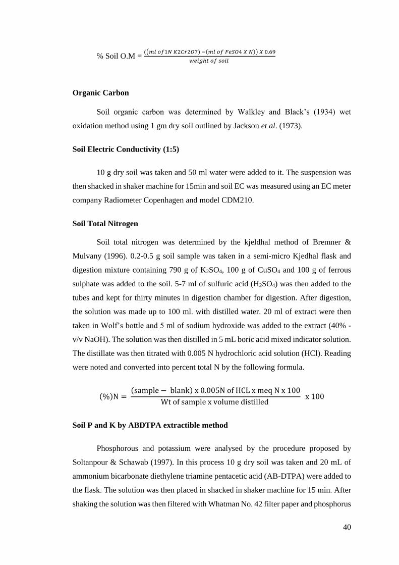
40
% Soil O.M = ((𝑚𝑙 𝑜𝑓1𝑁 𝐾2𝐶𝑟2𝑂7) −(𝑚𝑙 𝑜𝑓 𝐹𝑒𝑆𝑂4 𝑋 𝑁)) 𝑋 0.69
𝑤𝑒𝑖𝑔ℎ𝑡 𝑜𝑓 𝑠𝑜𝑖𝑙
Organic Carbon
Soil organic carbon was determined by Walkley and Black’s (1934) wet
oxidation method using 1 gm dry soil outlined by Jackson et al. (1973).
Soil Electric Conductivity (1:5)
10 g dry soil was taken and 50 ml water were added to it. The suspension was
then shacked in shaker machine for 15min and soil EC was measured using an EC meter
company Radiometer Copenhagen and model CDM210.
Soil Total Nitrogen
Soil total nitrogen was determined by the kjeldhal method of Bremner &
Mulvany (1996). 0.2-0.5 g soil sample was taken in a semi-micro Kjedhal flask and
digestion mixture containing 790 g of K2SO4, 100 g of CuSO4 and 100 g of ferrous
sulphate was added to the soil. 5-7 ml of sulfuric acid (H2SO4) was then added to the
tubes and kept for thirty minutes in digestion chamber for digestion. After digestion,
the solution was made up to 100 ml. with distilled water. 20 ml of extract were then
taken in Wolf’s bottle and 5 ml of sodium hydroxide was added to the extract (40% -
v/v NaOH). The solution was then distilled in 5 mL boric acid mixed indicator solution.
The distillate was then titrated with 0.005 N hydrochloric acid solution (HCl). Reading
were noted and converted into percent total N by the following formula.
(%)N = (sample − blank) x 0.005N of HCL x meq N x 100
Wt of sample x volume distilled x 100
Soil P and K by ABDTPA extractible method
Phosphorous and potassium were analysed by the procedure proposed by
Soltanpour & Schawab (1997). In this process 10 g dry soil was taken and 20 mL of
ammonium bicarbonate diethylene triamine pentacetic acid (AB-DTPA) were added to
the flask. The solution was then placed in shacked in shaker machine for 15 min. After
shaking the solution was then filtered with Whatman No. 42 filter paper and phosphorus

41
was analysed through spectrophotometer (520 nm) and potassium through flame
photometer.
Calcium Carbonate (CaCO3)
CaCO3 was analyzed by acid neutralization method of Black (1965).
DATA ANALYSIS
Soil data were statistically analysed using statistics 8.1 software two-way
ANOVA (LSD) was used to test for significant differences (P<0.05) for marginal
means of variables. Besides, Microsoft Excel spreadsheets were used for the
arrangement of data and their graphical representations.
3.4 SOCIO-ECONOMIC IMPACTS OF MONOCULTURE OF EXOTIC
TREE SPECIES
Necessary field visits were completed to collect the socio-economic data
through field observation and questionnaire surveys. Detailed information on socio-
economic condition in the study area in respect to monoculture woodlot of exotic trees
in public and private forests was collected. Observations on the following aspects
helped to cross check the collected information and data: (i) indigenous forest
management practices, (ii) wildlife and biodiversity, (iii) woodlot and Farm-forestry
plantations, (iv) local people attitude, (v) agricultural activities, (vi) land use pattern,
(viii) socio-economic activities, and (ix) others related activities.
At first, the necessary informal discussions with the local people on their
socioeconomic activities were conducted. These informal discussions helped to
generate successive questions for interview or further discussions. Accordingly, a
comprehensive semi-structured questionnaire modified after Rahman (2003) was
prepared. Finally, a detailed questionnaire survey and focus group discussion (FGD)
was carried out on the woodlot tree growers of the study areas in 2017-19 and the
necessary information was collected on different aspects of plantation. The number of
interviews as well as relevant data collection varied on the availability of the potential
interviewees, GO and NGOs organisational support and other circumstances.

42
Selection and Investigation of Woodlots and Tree Growers
Woodlots of exotic species Eucalyptus camaldulensis and Robinia
pseudoacacia raised on private land were selected from the study areas through
stratified random sampling and interviews were conducted accordingly. The
appropriate woodlots and respective households who were growing exotic trees or
practicing monoculture of exotic tree species in their own land with at least 0.25 ha (50
m x 50 m) land were searched through reconnaissance field visit and with the help of
local guides, local staffs of KPF&ED and local government authorities. Finally, a total
of 30 exotic woodlot tree growers at private level were selected from different areas of
District Malakand for data collection through a semi-structured questionnaire survey.
The questionnaire was composed of general information and woodlot/block
plantation (Appendix-19). The questionnaire surveys were conducted by a working
team led by the author and the data collected through face to face interviews. The goal
of each interview was to determine participants’ demographic and socio-economic
status as well as the expenditure or maintenance costs of and financial gains or profit
from the tree plantation plots. The tree growers who were cultivated the fast growing
exotic tree species as monoculture in their own land for quick economic return through
timber production were showed as per expenditure and income. The sample unit was
the household of the selected farmer who was involved as the respondent. Information
and data on growth performance of the woodlot trees were collected from the fields and
analysed accordingly. The current and future valuation of woodlots were determined in
consultation with local experts, forester, timber traders and tree growers.
Benefit Cost Analysis on the Woodlots Plantations of Exotic Tree Species
This study has assessed the costs and benefits of woodlot plantations. It focuses
on developing plantation system, followed by estimating the expenditure/costs and
benefits/revenue for the species planted. The costs projected here are based on ±10 year
(with different cycle of harvest depending on the species) rotation for one hectare’s
plantation of woodlot. Based on the costs and benefits estimated, the feasibility for the
woodlot plantation was examined. This feasibility analysis employed three main
economic tools, i.e. the net present value (NPV), benefit cost ratio (BCR) and internal
rate of return (IRR). A spreadsheet model (MS Excel 2016) was used to develop and
calculate the NPV, IRR and BCR.

43
Net Present Value
The term net present value is usually computed by finding the difference
between the present worth of the benefit stream minus the present worth of the cost
stream. The formula use for calculating the net present value is as below (Gittenger,
1974);
Net present value = Ʃ (Bt – Ct)/ (1 + i) t
Where, t = year, B = benefits, C = cost and i = discount rate.
Benefit Cost Ratio
Net present value tells us how much the expected present profit could be earned
from the investment but it does not reveal the proportion of total benefits against the
total costs invested. To do this, benefit cost ratio analysis is the right financial tool to
be employed. The following formula was used for calculating benefit costs ratio
(Gittenger, 1974):
Benefit costs ratio = Ʃ {Bt / (1 + i) t}/ Ʃ {Ct/(1 + i) t}
Where, t = year, B = benefits, C = cost and i = discount rate.
Internal Rate of Return
Apart from the net present value and benefit cost ratio analysis, internal rate of
return is another financial tool to determine the integrated planting. Internal rate of
return is measured when the discounted total benefits minus discounted total cost is
equal to zero. The investment should only be carried out if the internal rate of return is
more than capital cost interest rate (i.e. bank loan interest rate). The mathematical
formula for the above financial tools can be summarized as follow (Gittenger, 1974);
Internal rate of return = Ʃ {(Bt – Ct)/ (1 + i) t} = 0
Where, t = year, B = benefits, C = cost and i = discount rate.
Focus Group Discussion
In addition to the individual interviews and direct observation, FGD (a useful
Participatory Rural Appraisal-PRA technique) was also conducted to promote closer
interaction with the interviewees for obtaining more realistic responses. FGD were
separately held with the beneficiaries, tree growers, local people, timber traders and

44
related stakeholders. Gathering of focus groups consisting of local stakeholders living
within and nearby forests were organized by the working team led by the researcher.
The interviews were conducted at different places, preferably at local market (Bazar),
road sides, Hujras and other local community places where local people gathered
spontaneously.
The objectives of FGD were to-
(i) to collect specific information through consultation with local people, forest
villagers, businessman and resource user groups etc. (ii) to find out the socio-economic
impacts of exotic tree plantation in public and private land on rural livelihoods,
business, land use pattern and existing ecosystems.
During FGD, site specific information through consultation with local people,
forest villagers, tree growers, timber traders, different professional groups, resource
user groups (fuel wood collectors, sawmill owners), local public representatives and
government representatives (i.e. KPF&ED) were collected. This was basically through
informal interview but a checklist of issues was identified earlier and used as a basis
for questions. The following aspects were prioritized in FGD: (a) socio-economic and
ecological benefits/losses from the woodlot plantation of exotic species, (b) wildlife in
woodlot plantations and adjacent forests area, (c) potential timber tree species for
commercial woodlot plantations, (d) impacts of exotic tree species monoculture on
socio-economic and ecosystems.
Key Informant Interview
The purposes of this interview were to explore relevant data from different
corners and working groups. Questioning and discussion with key informants (i.e.
Divisional Forest Officer, Sub Divisional Forest Officer, Range Officer and Beat
Officer) were conducted on the traditional forest management system and wildlife
management, and woodlot plantation of exotic tree species at government forest land.
NGOs staff, teachers, government officers, union council chairman and members, and
local elites who provided important data on woodlots of exotic tree species, local
environment/ecosystem. A typical key interview lasted for about one hour and a
prepared checklist of questions was used for the purpose of interview.

45
Secondary Data Collection
Secondary data were collected from related literature and published documents
of government and non-government office for referring or supporting the findings.
Secondary data were collected to assess socio-economic impacts of monoculture of
exotic species, land use pattern, threats to native forests ecosystems and biodiversity.
Some demographic data and other related information were collected from Divisional
Forest Office in Malakand.
3.5. DISCHARGE RATE AND WATER TABLE MEASUREMENT
Three springs were selected randomly from each village. The discharge rate of
springs was measured by diverting the flow of water and passed through a small
hole/opening and the time was noted using a stop watch to fill a bottle of known volume
(300 m L and 1L). For big springs, an ordinary tape was used to measure average width
and depth while multiplying cross-sectional area and current speed (Q = VA). To find
out the speed, light floating object was thrown into the spring water and the time was
noted to cover a known distance. Past discharge rate were predicted by taking the marks
remained on rocks, an ordinary tape was used to measure the average width and depth,
the speed of water was assumed according to the topography of the spring. Water table
was measured using an ordinary tape, reaching it down to the water level in wells
(Kjelstrom, 1995).

46
CHAPTER - 4
RESULTS AND DISCUSSIONS
Khyber Pakhtunkhwa Forest Department and other national and international
organizations launched various types of forestry related projects in the province, in
which large scale plantations of the exotic tree species were carried out. The main
purpose of such plantations was to increase forest cover, reduce of poverty and improve
the livelihood of the local communities in the areas. They focused on establishment of
nurseries to produce the required numbers of seedling of fast growing exotic tree
species to gain economic returns. The existing natural forest is replaced by the
plantations and artificial regenerations of exotic fast growing species. The main
objectives of such projects were to increase the economic returns and ensure that
government strategies of management and policies adopt the same objectives as in the
previous years and is not detrimental to the remaining forests and ecosystems.
The monoculture of exotic species is a matter of great concerns when related to
sustainable development. The plantations of such species and their relative cost and
benefits are controversial subjects between the foresters and tree growers in terms of
social and environmental impacts. The introduction of fast growing species in
plantations projects poses threats to the sustainability of environment and therefore is a
matter of immense importance and is a subject of controversy between conservationists,
botanist, ecologist, foresters and policy makers.
Biodiversity loss and extinction of species may be the results of replacement of
indigenous species with the exotics directly or indirectly by affecting ecosystems. Most
people criticise the plantations as they threaten the habitat of the native forest plants
communities and by taking excessive water from the soil. In addition, ecological
problems were observed when indigenous species were cleared for the plantating of
exotic species (Hussain, 2002).
However, the activities of tree planting are important especially in our country
as the area under forest is lower than the required and the increasing poverty situation
leads to depletion of forests. People near forest area are compelled to cut trees and
overgraze these fragile areas.

47
The historical forestry review of Pakistan showed that the majority of the
projects were launched during the 1970s to 1980s which focused on plantations
establishment but failed to address management of natural forests. Large scale
plantations of exotic fast growing Eucalyptus camaldulensis and other species were
carried out to meet the fuel wood and timber requirements of the people.
No attention in the past has been paid to the ecological and socio-economic
impacts of plantation in District Malakand. This study assessed the ecological and
socio-economic impacts of the monoculture of two exotic tree species Eucalyptus
camaldulensis and Robinia pseudoacacia in comparison to that of indigenous tree
species of Pinus roxburghii and Acacia modesta in District Malakand.
The results of this study assesses the existing status of plant diversity, soil
properties, ground water and socio-economic impacts of monoculture of exotic tree
species on local economy and day to day life of the local people of the research area
have been presented in the following.
4.1. ECOLOGICAL IMPACTS
4.1.1. Undergrowth Vegetation
4.1.2. Floristic composition and Taxonomic Diversity
The plantations of exotic fast growing tree species affect the undergrowth
vegetation and plant diversity to a greater extent because of the invasive properties by
suppressing the indigenous plants species in terms of regenerations and growth. Though
the monoculture of some of the exotic species support the regenerations of the
indigenous species when protected and maintained their wilderness status in the
protected forest of the area. Other factors such as abundance of the planted species,
species types and ecology also affect the regeneration potential of the indigenous
vegetation. The negative impacts of exotic Eucalyptus could be mitigated by keeping
intact the understory vegetation in plantations to favour regeneration and normal plants
development (Liang and Qiang, 2009).
Floristic diversity, as defined by Ali et al. (2016), refers to the sum of all wild
and cultivated plants existing in any geographic area, which reveals the prevailing
climatic conditions, edaphic features, anthropogenic pressure and other natural stresses.

48
The result showed that flora of the research area consisted of a total of 174 plant species
belonging to 74 families and 150 genera, which were found in the selected research
plots of trees of indigenous (Pinus roxburghii, Acacia modesta) and exotic (Eucalyptus
camaldulensis and Robinia pseudoacacia) species. Among the recorded species 143
(82%) were dicotyledons, 26 (15%) species were monocotyledons and 4 (2.3%) were
pteridophytes while only 1 (0.7%) plant was recorded from gymnosperms. (Fig 4.1).
In indigenous plots of Pinus roxburghii, and Acacia modesta a total of 149
species of plants were recorded. Among the recorded species 120 (80%) were Dicots,
24 (16%) were monocots, 4 (3%) were pteridophytes and only 1 (1%) species was found
from gymnosperm as shown Fig. 4.2).
While in the exotic plots of Eucalyptus camaldulensis and Robinia
pseudoacacia a total of 111 species of plants were recorded. Among the recorded
species 93 (84%) were Dicots, 14 (12%) were monocots, 3 (3%) were pteridophytes
and only 1 (1%) species was found from gymnosperm as shown in Fig. 4.3).
Fig. 4.1. Taxonomic diversity of flora of all research plots.
143
25
4 1
174
0
20
40
60
80
100
120
140
160
180
200
Dicot Monocot Pteridophytes Gymnosperm Total
Nu
mb
er o
f sp
ecie
s
Taxonomic groups

49
Fig. 4.2. Taxonomic diversity of flora of indigenous research plots.
Fig. 4.3. Taxonomic diversity of flora of exotic research plots.
Ibrar and Hussain (2009) enlisted 100 ethnobotanical important plants from
Batkhela, District Malakand, which belonged to 49 families and among them 43
families were dicot, 2 of monocot, 2 of pteridophytes, and 1 of gymnosperms.
Barkatullah & Ibrar (2011) reported a total of 169 plant species belonging to 140 genera
and 76 families from Malakand Pass hills. They were represented by 63 dicot families,
5 monocots, 4 pteridophytes and only 1 gymnosperm family. Zabihullah et al. (2006)
documented a total of 82 plant species and their uses for various purposes from kot
Manzaray Baba valley Malakand agency. They found that among these plants 65%
were medicinal, 20% were used for fuelwood, 6% for honeybees, 8% for fruit, 9% for
120
24
4 1
149
0
20
40
60
80
100
120
140
160
Dicot Monocot PteridophytesGymnosperm Total
Nu
mb
er o
f sp
ecie
s
Taxonomic groups
93
14
3 1
111
0
20
40
60
80
100
120
Dicot Monocot Pteridophytes Gymnosperm Total
Nu
mb
er o
f sp
ecie
s
Taxonomic groups

50
timber and 7% as potherb. They also reported that the area is under heavy biotic
pressure of deforestation and overgrazing. Zaman et al. (2013) carried out
ethnobotanical survey of the plant species in Tehsil Dargai and a total of 40 plants were
collected which were represented by 26 families. Out of these 40 plants 12 were trees
and 18, were herbs, 7 were shrubs and 2 were climbers. Muhammad et al. (2016) found
that Dodonea viscosa (L.) Jacq was the dominant shrub species in terms of density and
percent cover. In addition, percent species and abundance show contrast variations with
relative frequency. Muhammad et al. (2016) studied the ethno-botanical importance of
the understorey plants species in Acacia modesta forest of Malakand Division. He
observed that species, such as Vitex negundo, Dodonea viscosa, Zizypus
nummularia and Mallotus philippinensis, were cut down regularly without any
conservation measure. Dogra et al. (2009) carried out comparative study of plant
diversity in exotic and indigenous tree forest. They found that the numbers of plant
species in the plantations of indigenous Pinus roxburghii Sarg. were greater compared
to the exotic Eucalyptus citriodora Hook. Plantations. Khan et al. (2017) reported 264
plants represented by 90 families and 202 genera of which 42 were monocots and 216
were dicots from Tehsil Swat ranizai of District Malakand. Among them 172 plant
species were perennials and 86 were annuals while only 6 species were biennial.
In this research, 174 plants species belonging to 74 families and 150 genera,
were found in the selected research plots of trees of indigenous (Pinus roxburghii,
Acacia modesta) and exotic (Eucalyptus camaldulensis and Robinia pseudoacacia)
origin. Among the recorded species 143 (82%) were dicotyledons, 26 (15%) species
were monocotyledons and 4 (2.3%) were pteridophytes while only 1 (0.7%) plant was
recorded from gymnosperms. (Fig 4.1).
In indigenous plots 149 species of plants were recorded. Among the recorded
species 120 (80%) were Dicots, 24 (16%) were monocots, 4 (3%) were pteridophytes
and only 1 (1%) species was found from gymnosperm as shown Fig. 4.2. In the exotic
plots 111 species of plants were recorded. Among the recorded species 93 (84%) were
Dicots, 14 (12%) were monocots, 3 (3%) were pteridophytes and only 1 (1%) species
was found from gymnosperms as shown Fig. 4.3. The number of uncommon species
were higher in indigenous plots as compared to the exotic plots facing similar extent of
ecological and anthropogenic stresses. This scenario proves that plantations of

51
indigenous species are relatively better in harbouring better species richness and
diversity.
Morphological diversity of the plants of the research plots showed that among
the total 174 plant of all species plots 29 (17%) consisted of trees, 31 (18%) of shrubs,
86 (49%) of herbs, 19 (11%) of grasses, 6 (3.3%) of climbers and only 3 (1.7%)
consisted of sedges (Fig. 4.4).
In indigenous plots a total of 23 (15%), 30 (20%), 74 (50%), 16 (11%), 3 (2%),
3 (2%) were represented by trees, shrubs, herbs, grasses, climbers and sedges
respectively (Fig.4.5).
While in exotic plots a total of 18 (16%) trees, 18 (16%)shrubs, 57 (51%) herbs,
11 (10%) grasses, 5 (5%) climbers and 2 (2%) sedges were recorded (Fig. 4.6).
Fig. 4.4. Morphological diversity of plants species of all plots.
29 31
86
19
6 3
174
0
20
40
60
80
100
120
140
160
180
200
Trees Shrubs Herbs Grasses Climbers Sedges Total
Nu
mb
er o
f p
lan
ts
Morphological diversity groups

52
Fig. 4.5. Morphological diversity of plants species of indigenous plots.
Fig. 4.6. Morphological diversity of plants species of exotic plots.
Based on the life span of the plant species a total of 119 (68%) plants were found
to be perennials, 54 (31%) were found to be annuals and only 1 (1%) plants were
recorded biennial among all the 174 plants in all the research plots of the study area
(Fig. 4.7).
Among the 149 plants of the indigenous plots 108 (72%) were perennials, 41
(28%) were annuals while no plant was recorded as biennials (fig. 4.8). While in the
exotic plots, among 111 plants, 74 (67%), 36 (32%) and 1 (1%) were recorded as
perennials, annuals and biennials respectively (Fig. 4.9).
2330
74
163 3
149
0
20
40
60
80
100
120
140
160
Trees Shrubs Herbs Grasses Climbers Sedges Total
Nu
mb
er o
f p
lan
ts
Morphological diversity groups
18 18
57
115 2
111
0
20
40
60
80
100
120
Trees Shrubs Herbs Grasses Climbers Sedges Total
Nu
mb
er o
f p
lan
ts
Morphological diversity groups
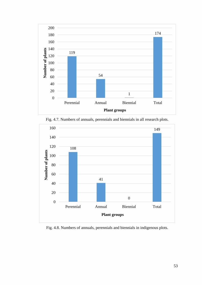
53
Fig. 4.7. Numbers of annuals, perennials and biennials in all research plots.
Fig. 4.8. Numbers of annuals, perennials and biennials in indigenous plots.
119
54
1
174
0
20
40
60
80
100
120
140
160
180
200
Perennial Annual Biennial Total
Nu
mb
er o
f p
lan
ts
Plant groups
108
41
0
149
0
20
40
60
80
100
120
140
160
Perennial Annual Biennial Total
Nu
mb
er o
f p
lan
ts
Plant groups

54
Fig. 4.9. Numbers of annuals, perennials and biennials in exotic plots.
It is clear from the Fig. 4.10. that the number of all undergrowth species in Pinus
roxburghii plots in spring, monsoon and winter were 83,83 and 62 respectively. while
in Acacia modesta plots total of 89, 89 and 67 plants species were present in spring,
monsoon and winter seasons respectively.
Fig. 4. 10. Species composition in different tree plots in spring, monsoon and winter
seasons in the study area.
74
36
1
111
0
20
40
60
80
100
120
Perennial Annual Biennial Total
Nu
mb
er o
f p
lan
ts
Plants group
8389
70 67
8389
70 6762 6758
34
0
20
40
60
80
100
Pinus roxburghii
Plots
Acacia modesta
Plots
Eucalyptus
camaldulensis
Plots
Robinia
pseudoacacia
Plots
Nu
mb
er o
f sp
ecie
s
Plants
Considering all undergrowths species
spring Monsoon winter

55
Similarly, in Eucalyptus camaldulensis plots 70 each in spring and monsoon
and 58 species were recorded during spring, monsoon and winter respectively. While
67 species each in spring and monsoon and 34 plants species of all undergrowths were
recorded during winter in Robinia pseudoacacia plots.
During this study, considering all undergrowth plants a total of 149 species
including 23 tree species were found combined in all indigenous plots in all seasons
whereas 111 undergrowth species including 18 tree species occurred in all exotic plots
in all seasons. (Fig. 4.11).
Fig.4.11. Showing number of all undergrowth plants and number of tree species in
exotic and indigenous research plots.
The findings showed that maximum numbers of plants of all undergrowth were
present in indigenous plots as compared to the exotic plots in the study area. Similarly,
a greater number of trees species were present in indigenous plots as compared to the
exotic plots of the study area.
Maximum number of trees species were found in indigenous Pinus roxburghii
plots which was followed by indigenous Acacia modesta plots and the number of tree
species were 15 and 13 respectively. While 10 tree species were found in both exotic
Eucalyptus camaldulensis and Robinia pseudoacacia plots respectively. Hence 23 tree
species in total were recorded in indigenous plots while 18 species occurred combined
in exotic plots as shown in (Fig.4.12).
111
18
149
23
0
20
40
60
80
100
120
140
160
Number of all undergrowth plants
species
Number of tree species only
Nu
mb
er o
f p
lan
ts
Plants
Exotic Plots Indigenous Plots
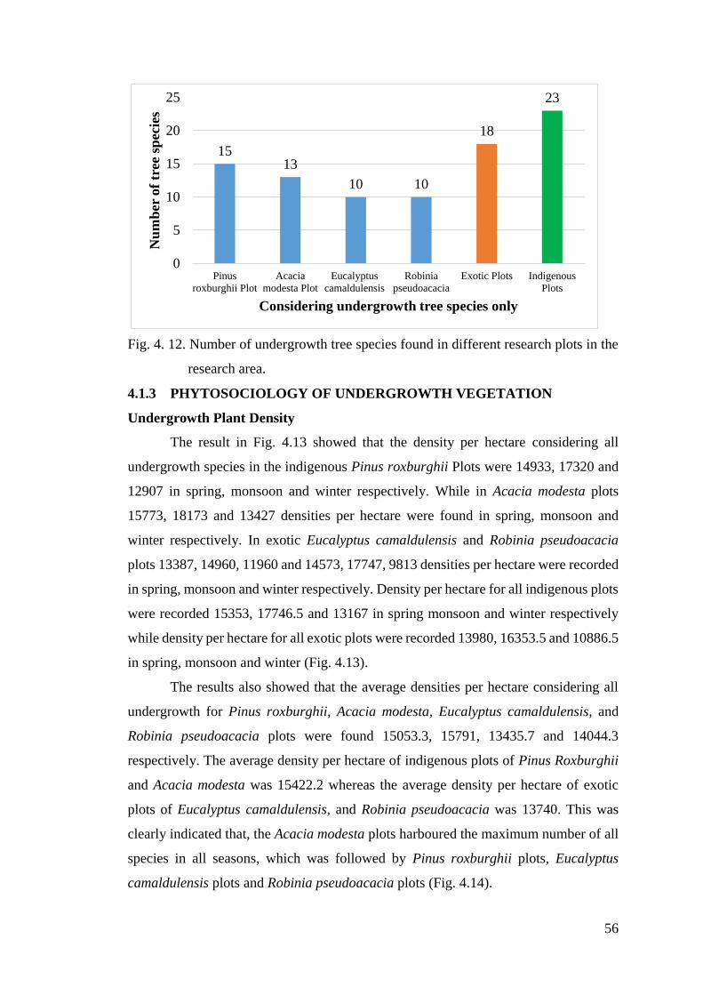
56
Fig. 4. 12. Number of undergrowth tree species found in different research plots in the
research area.
4.1.3 PHYTOSOCIOLOGY OF UNDERGROWTH VEGETATION
Undergrowth Plant Density
The result in Fig. 4.13 showed that the density per hectare considering all
undergrowth species in the indigenous Pinus roxburghii Plots were 14933, 17320 and
12907 in spring, monsoon and winter respectively. While in Acacia modesta plots
15773, 18173 and 13427 densities per hectare were found in spring, monsoon and
winter respectively. In exotic Eucalyptus camaldulensis and Robinia pseudoacacia
plots 13387, 14960, 11960 and 14573, 17747, 9813 densities per hectare were recorded
in spring, monsoon and winter respectively. Density per hectare for all indigenous plots
were recorded 15353, 17746.5 and 13167 in spring monsoon and winter respectively
while density per hectare for all exotic plots were recorded 13980, 16353.5 and 10886.5
in spring, monsoon and winter (Fig. 4.13).
The results also showed that the average densities per hectare considering all
undergrowth for Pinus roxburghii, Acacia modesta, Eucalyptus camaldulensis, and
Robinia pseudoacacia plots were found 15053.3, 15791, 13435.7 and 14044.3
respectively. The average density per hectare of indigenous plots of Pinus Roxburghii
and Acacia modesta was 15422.2 whereas the average density per hectare of exotic
plots of Eucalyptus camaldulensis, and Robinia pseudoacacia was 13740. This was
clearly indicated that, the Acacia modesta plots harboured the maximum number of all
species in all seasons, which was followed by Pinus roxburghii plots, Eucalyptus
camaldulensis plots and Robinia pseudoacacia plots (Fig. 4.14).
1513
10 10
18
23
0
5
10
15
20
25
Pinus
roxburghii Plot
Acacia
modesta Plot
Eucalyptus
camaldulensis
Robinia
pseudoacacia
Exotic Plots Indigenous
Plots
Nu
mb
er o
f tr
ee s
pec
ies
Considering undergrowth tree species only

57
Somewhat similar finding was found by Muhammad et al. 2016 in studying
density and diversity of understory vegetation in relation to site conditions in natural
stands of Acacia modesta from malakand division. Densities per hectare recorded for
Otostegia limbata, Justicia adhatoda, Carthamus oxycantha, Chenopodium
album,Cannabis sativa, Cymbopogon distans, Conyza Canadensis, Cenchrus ciliaris,
Parthenium hysterophorus, Solanum nigrum, Saccharum griffthii and Tagetes minuta
occurred with a mean density ranging from 100-460 individuals per ha, and that
Zizyphus nummularia, Nerium indicum, Datura innoxia, Calotropis procera, Daphne
oleoides, Vitex negundo, Grewia optiva, Verbascum thapsus, Amaranthus viridis,
Ajuga bracteosa shared a mean density of 1.25-85 individuals per hectare.
The difference in the density of plants species per hectare and species diversity
may be due to the changes in environmental conditions i.e. light and nutrients
availabilty. In exotic species plantations large and homogenous canopy was formed
with less gaps and because of fast growth of dominant tree species in the plots as shown
in Table 4.3 utilized more soil nutrients. While in indigenous plots the increase numbers
of plants species may be due to the non uniform canopy and the light reached the soil
due to which the regeneration of the understorey vegetations has been affected
differently (Uemura, 1994). The greater densities of plants in the indigenos plots of
species may be due the greater amount of organic matter in the indigenous plots which
produced and returned large amount of litter (Sevgi and Tecimen, 2008). The nutrients
released from litter decomposition were more in indigenous species plots as shown in
Table-4.4 and 4.5 indicated that the soil nutrients like N, P, K, OM, OC was more in
indigenous species plots than exotic species plots.

58
Figure 4.13. Undergrowth densities per hectare considering all undergrowth species in
three seasons in different research plots in the study area.
Fig. 4.14. Average undergrowth density per hectare considering all undergrowth
species in different tree plots in research area.
Relative Density
Considering all undergrowth species, the highest relative density was found in
exotic plots for Dodonaea viscosa (10.42%), followed by Robinia pseudocacia
(7.16%), Eucalyptus camaldulensis (6.81%), Chrysopogon aucheri (3.99%), Olea
0
2000
4000
6000
8000
10000
12000
14000
16000
18000
20000
Pinus
roxburghii
Plot
Acacia
modesta Plot
Eucalyptus
camaldulensis
Plot
Robinia
pseudoacacia
Plot
Exotic Plots Indigenous
Plots
Den
sity
/hec
in
dif
fere
nt
seaso
ns
Plants
spring Monsoon winter
15053.3
15791
13435.7
14044.313740
15422.2
12000
12500
13000
13500
14000
14500
15000
15500
16000
Pinus
roxburghii
Plot
Acacia
modesta Plot
Eucalyptus
camaldulensis
Plot
Robinia
pseudoacacia
Plot
Exotic Plots Indigenous
Plos
Den
sity
/hec
of
pla
nts
Plants

59
ferruginea (3.84%), Cannabis sativa (2.71%), Symphyotrichum graminifolium
(2.65%), Saccharum filifolium (2.24%). The lowest relative density (0.06%), was found
for Barleria cristata, Calistemin lanceolatus, Caralluma tuberculate, Colebrookea
oppositifolia, Daphne oleoides, Isodon rugosus, Melothria heterophylla, Mentha
longifolia, Peganum harmala, Quercus incana, Rhazya stricta and Salix babylonica
(Appendix-3).
While among the indigenous plots, the relative density was found to be greatest
for Dodonea viscosa (9.26%), Acacia modesta (8.12%), Pinus roxburghii (6.38%),
Chrysopogon aucheri (4.33%), Olea ferruginea (4.15%), Aristida cyanantha (2.26%),
Launaea procumbens (1.97%), Ficus palmata (1.87%). The lowest relative density
(0.05%) was recorded for Colebrookea oppositifolia, Ehretia obtusifolia, Melothria
heterophylla, Mentha longifolia, Monotheca buxifolia, Myrsine africana, Periploca
aphylla, Quercus incana, Solanum surattense, Tecomella undulata, Teucrium
stocksianum and Ziziphus nummularia (Appendix-2).
On the other hand, considering only the seedlings and saplings of the trees
species as the undergrowth, the relative density in the exotic plots was found to be
highest for Robinia pseudocacia (24.8%), Eucalyptus camaldulensis (23.59%), Olea
ferruginea (13.3%), Acacia modesta (6.65%), Mallotus philippensis (6.25%),
Broussonetia papyrifera (5.14%). The lowest relative density (0.2%) was recorded for
Calistemin lanceolatus, Quercus incana and Salix babylonica (Appendix-5).
In indigenous plot the relative density was found to be highest in Acacia
modesta (26.87%), Pinus roxburghii (21.12%), Olea ferruginea (13.73%), Ficus
palmata (6.18%), Mallotus philippensis (5.58%). The lowest relative density (0.17%)
was found for Monotheca buxifolia, Quercus incana and Tecomella undulata
(Appendix-4).
The density of naturally emergent seedlings is mostly damaged due to the
clearing of undergrowth on forest floor, grazing and trampling, and the collection of
leaf litter which were found in the research arae (Kotilouoto and Makandi, 2004).

60
Frequency
Considering all undergrowth species, the highest frequency was found in exotic
plots for Dodonaea viscosa (80%), followed by Olea ferruginea (53.3%), Eucalyptus
camaldulensis (50%), Robinia pseudocacia (48.3%), Pinus roxburghii (25%), Ficus
palmata (25%), Mallotus philippensis (21.6%), Chrysopogon aucheri (21.6%). The
lowest frequency (1.1%) was recorded for Ammi visnaga, Convolvulus arvense,
Heliotropium strigosum, Lathyrus cicera, Malva neglecta, Medicago minima, Papaver
pavoninum, Peganum harmala, Trichodesma indica and Xanthium sibiricum
(Appendix-3).
While among the indigenous plots, frequency was found to be greatest for Olea
ferruginea (78.3%), Dodonea viscosa (73.3%), Acacia modesta (68.3%), Pinus
roxburghii (45%), Ficus palmata (41.6%), Celtis caucasica (40%), Grewia optiva
(28.3%). The lowest frequency (1.1%) was calculated for Martynia annua, Medicago
minima, Oxalis corniculata, Peganum harmala and Plantago major (Appendix-2).
While on the other hand, considering only the seedlings and saplings of the trees
species as the undergrowth, the frequency in the indigenous plot is found to be highest
for Olea ferruginea (78.3%), Acacia modesta (68.3%), Pinus roxburghii (45%), Ficus
palmata (41.6%), Celtis caucasica (40%). The lowest frequency (1.6%), was found for
the Monotheca buxifolia, Quercus incana and Tecomella undulata (Appendix-4).
In exotic plots the frequency was found to be highest for Olea ferruginea
(53.3%), Eucalyptus camaldulensis (50%), Robinia pseudocacia (48.3%), Pinus
roxburghii (25%), Ficus palmata (25%). The lowest frequency (1.6%), was found for
Calistemin lanceolatus, Quercus incana and Salix babylonica (Appendix-5).
Relative Frequency
Considering all undergrowth species, the highest relative frequency was found
in exotic plots for Dodonaea viscosa (8.3%), followed by Olea ferruginea (5.53%),
Eucalyptus camaldulensis (5.19%), Robinia pseudocacia (5.01%), Ficus palmata
(2.59%), Pinus roxburghii (2.59%), Chrysopogon aucheri (2.25%). The lowest relative
frequency (0.12%), was found for Ammi visnaga, Convolvulus arvense, Heliotropium
strigosum, Lathyrus cicera, Malva neglecta, Medicago minima, Papaver pavoninum,
Peganum harmala, Trichodesma indica and Xanthium sibiricum (Appendix-3).

61
While among the indigenous plots, the relative frequency was found to be
greatest for Olea ferruginea (6.3%), followed by Dodonea viscosa (5.92%), Acacia
modesta (5. 52%), Pinus roxburghii (3.64%), Ficus palmata (3.37%), Celtis caucasica
(3.23%). The lowest relative frequency (0.09%) was found for Martynia annua,
Medicago minima, Oxalis corniculata, Peganum harmala and Plantago major
(Appendix-2).
On the other hand, considering only the seedlings and saplings of the trees
species as the undergrowth, the relative frequency in the exotic plots was found to be
highest for Olea ferruginea (17.1%), followed by Eucalyptus camaldulensis (16.04%),
Robinia pseudocacia, (15.5%), Pinus roxburghii (8.02%), Ficus palmata (8.02%),
Mallotus philippensis (6.95%). The lowest relative frequency (0.54%), was found for
Calistemin lanceolatus, Quercus incana and Salix babylonica (Appendix-5).
In indigenous plots the relative frequency was found to be highest in Olea
ferruginea (17.03%), Acacia modesta (14.8%), Pinus roxburghii (9.78%), Ficus
palmata (9.06%), Celtis caucasica (8.7%), Grewia optiva (6.1%). The lowest relative
frequency (0.36%) was found for Monotheca buxifolia, Quercus incana and Tecomella
undulata (Appendix-4).
Abundance
Considering all undergrowth species, the highest relative abundance was found
in exotic plots for Avena fatua (10.5%), followed by Commelina paludosa (9.17%),
Symphyotrichum graminifolium (9.06%), Dryopteris crenata (7.4%), Heteropogon
contortus (7%), Aerva sanguinolenta (6.8%). The lowest abundance (1%) was found
for Barleria cristata, Calistemin lanceolatus, Caralluma tuberculata, Colebrookea
oppositifolia, Dalbergia sissoo, Daphne oleoides, Datura innoxia, Duchesnea indica,
Isodon rugosus, Maytenus royaleana, Melothria heterophylla, Mentha longifolia,
Nannorrhops ritchiana, Opuntia monacantha, Periploca aphylla, Quercus incana,
Rhazya stricta, Sageretia thea, Salix babylonica and Withania coagulans (Appendix-
3).
While among the indigenous plots, abundance was found to be greatest for
Chrysopogon serrulatus (9%), Apluda mutica (8.5%), Dryopteris jaxtaposta and
Imperata cylindrica (8%), Chrysopogon aucheri (7.14%), Adiantum caudatum,

62
Stipagrostis hirtigluma (6.67%) for each one. The lowest abundance (1%) was found
for Albizia lebbeck, Berberis lyceum, Buddleja crispa, Caralluma tuberculata,
Cissampelos pareira, Colebrookea oppositifolia, Daphne oleoides, Datura innoxia,
Desmodium elegans, Ehretia obtusifolia, Lotus corniculatus, Maytenus
royaleana, Melothria heterophylla, Mentha longifolia, Monotheca buxifolia, Myrsine
Africana, Nannorrhops ritchiana, Periploca aphylla, Punica granatum, Quercus
incana, Sageretia thea, Solanum surattense, Tecomella undulata and Teucrium
stocksianum (Appendix-2).
On the other hand, considering only the seedlings and saplings of the trees
species as the undergrowth, the abundance in the exotic plots was found to be highest
for Broussonetia papyrifera (6.07%), followed by Robinia pseudocacia (5.08%),
Eucalyptus camaldulensis (4.6%), Acacia modesta (3.3%), Mallotus philippensis
(2.8%). The lowest abundance (1%) was found for Calistemin lanceolatus, Dalbergia
sissoo, Quercus incana and Salix babylonica. (Appendix-5).
In indigenous plot the abundance was found to be highest in Pinus roxburghii
(5.46%), Acacia modesta (4.59%), Mallotus philippensis (3.25%), Pistacia chinensis
(3%), Bauhinia variegata (2.4%), Olea ferruginea (2.04%), Ziziphus mauritiana (2%).
The lowest abundance (1%), was found for Albizia lebbeck, Monotheca buxifolia,
Punica granatum, Quercus incana and Tecomella undulata (Appendix-4).
Relative Abundance
Considering all undergrowth species, the highest relative abundance was found
in exotic plots for Avena fatua (2.9%), Commelina paludosa (2.6%),
Symphyotrichum graminifolium (2.5%), Dryopteris crenata (2%), Heteropogon
contortus (1.9%), Aerva sanguinolenta (1.9%). The lowest (0.28%), relative abundance
was found for Barleria cristata, Calistemin lanceolatus, Caralluma tuberculata,
Colebrookea oppositifolia, Dalbergia sissoo, Daphne oleoides, Datura innoxia,
Duchesnea indica, Isodon rugosus, Maytenus royaleana, Melothria heterophylla,
Mentha longifolia, Nannorrhops ritchiana, Opuntia monacantha, Periploca aphylla,
Quercus incana, Rhazya stricta, Sageretia thea, Salix babylonica and Withania
coagulans (Appendix-3).

63
While among the indigenous plots, the relative abundance was found to be
greatest for Chrysopogon serrulatus (2.06%), Apluda mutica (1.94%), Dryopteris
jaxtaposta and Imperata cylindrica (1.83%), Adiantum caudatum, Cenchrus ciliaris
and Stipagrostis hirtigluma (1.52%), Saccharum filifolium (1.49%), Poa annua
(1.46%). The lowest relative abundance (0.23%), was found for Albizia lebbeck,
Berberis lyceum, Buddleja crispa, Caralluma tuberculata, Cissampelos pareira,
Colebrookea oppositifolia, Daphne oleoides, Datura innoxia, Desmodium
elegans, Ehretia obtusifolia, Lotus corniculatus, Maytenus royaleana, Melothria
heterophylla, Mentha longifolia, Monotheca buxifolia, Myrsine Africana,
Nannorrhops ritchiana, Periploca aphylla, Punica granatum, Quercus incana,
Sageretia thea, Solanum surattense, Tecomella undulata and Teucrium stocksianum
(Appendix-2).
On the other hand, considering only the seedlings and saplings of the tree
species as the undergrowth, the relative abundance in the exotic plot was found to be
greatest for Broussonetia papyrifera (13.7%), Robinia pseudocacia (11.5%),
Eucalyptus camaldulensis, (10.6%), Acacia modesta (7.5%), Mallotus philippensis
(6.46%). The lowest relative abundance (2.2%), was found for Calistemin lanceolatus,
Dalbergia sissoo Quercus incana and Salix babylonica (Appendix-5).
In indigenous plot the relative abundance was found to be highest in Pinus
roxburghii (12.3%), Acacia modesta (10.3%), Mallotus philippensis (7.3%), Pistacia
chinensis (6.7%), Bauhinia variegata (5.4%), Olea ferruginea (4.6%). The lowest
relative abundance value (2.26%), was found for the Albizia lebbeck, Monotheca
buxifolia, Punica granatum, Quercus incana and Tecomella undulata (Appendix-4).
Communities structure
The following plant communities were reported from the study of different species plots
in the research area.
1. Pinus-Dodonea-Olea Community
Pinus-Dodonea-Olea community was reported from the study plots of Pinus
roxburghii. Pinus roxburghii, Dodonea viscosa and Olea ferruginea were dominant
species with importance values of 23.07, 14.4 and 9.64 respectively. Mallotus

64
philippensis was co-dominant tree species with importance value 7.37 and the
associated species were Chrysopogon aucheri (8.02), Dryopteris jaxtaposta (8.09),
Dryopteris crenata (6.60), Launaea procumbens (6.10) and Aristida cyanantha (5.77).
2. Eucalyptus-Dodonea- Acacia Community
Eucalyptus-Dodonea- Acacia community was reported from the study plots of
Eucalyptus camaldulensis. Eucalyptus camaldulensis, Dodonea viscosa and Acacia
modesta were dominant species with importance values of 25.8, 22.8 and 9.48
respectively. Mallotus philippensis was co-dominant tree species with importance value
9.27 and the associated species were Dryopteris crenata (9.28), Olea ferruginea (9.08),
Adiantum caudatum (8.74), Pinus roxburghii (8.46), Chryspogan aucheri (7.68),
Aristida cyanantha (7.61%), Cymbopogon jwarancusa (7.15) and Symphyotrichum
graminifolium (7.09).
3. Acacia- Dodonea-Olea Community
Acacia- Dodonea-Olea community was reported from the study plots of Acacia
modesta. Acacia modesta, Dodonea viscosa and Olea ferruginea were dominant
species with importance values of 23.9, 19.6 and 12.79 respectively. Grevia optiva and
Ficus palmata were co-dominant trees species while the associated species were
Chryspogan aucheri (10.04), Justicia adhatoda (7.48), Saccharum filifolium (7.49),
Cymbopogon jwarancusa (6.35) and Aristida cyanantha (5.90).
4. Robinia-Dodonea-Olea Community
Robinia-Dodonea-Olea community was reported from the study plots of Robinia
pseudoacacia. Robinia pseudoacacia, Dodonea viscosa, Olea ferruginea were
dominant species with importance values of 27.18, 18.8 and 12.4 respectively.
Broussonetia papyrifera was the co-dominant tree species and the associated species
were Chrysopogon aucheri (10.36), Cannabis sativa (8.66), Symphyotrichum
graminifolium (8.53), Saccharum filifolium (7.76). Aerva sanguinolenta (7.72).
Carthamus lanatus (7.57), Euphorbia hirta (6.97) and Parthenium hysterophorus
(6.83).
4.1.4. Phytodiversity Index
In this research, the values of Shannon- wiener diversity index were calculated
(appendixes 6.1-6.24) and was statistically analysed in (appendixes 6.25-6.28) and

65
presented in the Table-4.1 and Table-4.2 respectivey.
Table-4.1: Table showing Shannon-Wiener diversity index values recorded for
different research plots.
Name of
season All undergrowth species Undergrowth tree species only
Pinus
roxburghii
Acacia
modesta
Eucalyptus
camaldulensis
Robinia
pseudoacacia
Pinus
roxburghii
Acacia
modesta
Eucalyptus
camaldulensis
Robinia
pseudoacacia
Spring 3.9 3.7 3.5 3.6 2.01 1.77 1.72 1.5 Monsoon 3.95 3.8 3.4 3.7 2.01 1.8 1.76 1.55 Winter 3.6 3.4 3.3 3 2.01 1.77 1.72 1.5 Average 3.83 3.63 3.4 3.43 2.01 1.78 1.73 1.51 Name of
season All undergrowth species Undergrowth tree species only
Indigenous
Plots
Exotic Plots Indigenous
Plots
Exotic Plots
Spring 3.8 3.55 1.9 1.61 Monsoon 3.9 3.55 1.9 1.65 Winter 3.5 3.15 1.89 1.61 Average 3.73 3.14 1.9 1.62
Considering all undergrowth species of all research plots, the value of Shannon-
Wiener diversity index (H) was found to vary between 3.83 to 3.40, where the highest
value 3.95 was recorded from Pinus roxburghii plots in monsoon season and the lowest
value 3 was from Robinia pseudoacacia plot in winter season. The highest mean value
(3.833) of Shannon-Wiener diversity index (H) was found in Pinus roxburghii Plots,
followed by Acacia modesta Plots, Robinia pseudoacacia Plots, and Eucalyptus
camaldulensis Plots and their index values are 3.633, 3.4333 and 3.40 respectively. The
mean value 3.83 of Shannon-Wiener diversity index (H) was recorded as the highest
for indigenous plots, whereas the lowest value 3.40 was recorded for exotic plots. The
data from the Shannon-Wiener diversity index (H) calculated for four types of plots
showed the following pattern in four types of tree plots- Pinus roxburghii > Acacia
modesta > Robinia pseudoacacia > Eucalyptus camaldulensis.
The result of this study on species diversity indicated that indigenous tree plots
harbour greater numbers of plants and are more diverse as compared to the exotic plots
which were having relatively less plants. These observations were supported by similar
surveys undertaken by Kohli (1998): Dogra et al. (2009) and Montagnini et al., (2005).
Greater diversity of different plant groups existed in the indigenous Acacia modesta
and Pinus roxburghii despites the area faced collection of leaf litter, fuelwood and
illegal cutting of trees and grazing pressure.

66
On the other hand, considering only the seedlings and saplings of tree species
as undergrowth, the greater mean value 2.01 was found for Pinus roxburghii Plots,
which was followed by 1.78, 1.73, 1.51 for Acacia modesta Plots, Eucalyptus
camaldulensis Plots and Robinia pseudoacacia Plots respectively. The highest mean
value 2.01 was found in indigenous plots while the lowest value 1.51 occurred in exotic
plots. The mean values of Shannon-Wiener diversity index calculated for the seedlings
and saplings of all tree species as undergrowth in all of the four plots followed the given
pattern Pinus roxburghii Plots > Acacia modesta Plots > Eucalyptus camaldulensis
Plots > Robinia pseudoacacia Plots with the index values 2.01,1.78, 1.73, 1.51
respectively.
Table-4.2. Mean values of Shannon- weiner diversity index of different research plots
calculated after analysis using statistics 8.1 software two-way ANOVA (LSD) was
used to test for significant differences (P<0.05) for marginal means of variables.
Mean values with different alphabet letters shows significanct difference at p < 0.05.
It is clear from the table 4.2 that the highest Shannon-Wiener Diversity index
value (H) was found for Indigenous plots with the index value of 3.73 while the lowest
value 3.41 was found for all exotic plots when all undergrowth species were considered.
While considering only the seedlings and saplings of tree species of undergrowth the
highest index value (1.89) was recorded for indigenous plots followed by exotic plots
(1.62).
4.1.5. Tree productivity
The detail data related to tree productivity which included trees density per hectare,
trees height, DBH, basal area and tree stem volume in the plots of different exotic and
indigenous species are presented below.
Treatments All undergrowth species
Undergrowth tree species
only
PLANTS
Pinus roxburghii Plots 3.833 a 2.01 a
Acacia modesta Plots 3.633 ab 1.78 b
Eucalyptus camaldulensis
Plots 3.4000 b 1.73 c
Robinia pseudoacacia Plots 3.4333 b 1.51 d
LSD 0.25 0.02
Exotics vs Indigenous
Exotic 3.73 1.89
Indigenous 3.41 1.62
Significance significant Significant

67
Table-4.3: Density of trees, height, DBH, basal area and gross tree stem volume
in different plots of exotic and indigenous species.
Types of plots Density/hac Height
(m)
DBH
(cm)
Basal Area
(m2/hac)
Gross tree
stem volume
(m3/hac)
E. camaldulensis 995 12 23 41 778
R. pseudoacacia 1010 5 21 35 274
Exotic species
plots (average) 1002 8.5 22 38 526
A. modesta 1130 5 20 35 278
P. roxburghii 960 10 20 30 473
Indigenous species
plots (average) 1045 7.5 20 32 375
It is evident from the data given in Table-4.3 that the number of trees per hectare
in the plots of E. camaldulensis, R. pseudoacacia, A. modesta, P. roxburghii were 995,
1010, 1130 and 960 respectively. The average number of trees in the exotic and
indigenous plots of species were 1002 and 1045 respectively which indicated that the
average number of trees per hectare in the exotic species plots and indigenous species
plots were not much differet. Mean height of trees in the exotic species plots was
maximum (8.5 m) whereas it was lower (7.5 m) in the Indigenous species plots. The
increased height of trees in the exotic plots indicated that the exotic species grown
rapidly and gain sufficient heigh because of their fast growing nature. The indigenous
species gain low height because they were slow growing.
The result showed that maximum (22 cm) DBH was recorded in exotic species
plots and low (20 cm) in indigenous species plots. It is clear from the DBH data that
the exotic species gain maximum diameter due to fast growth and the indigenous
species gained relatively less diameter because of slow growth. The result showed that
basal area recorded from the plots of exotic species was more (38 m2/hac) as compared
to indigenous species plots (32 m2/hac). Greater basal area of the exotic species plots
showed that canopies of trees covered much of the the area of ground as compared to
the the indigenous species plots. Gross tree stem volume recorded from the exotic
species plots were maximum (526 m3/hac) whereas the it was lower (375 m3/hac) in
indigenous species plots which indicated that the exotic species plots produced more
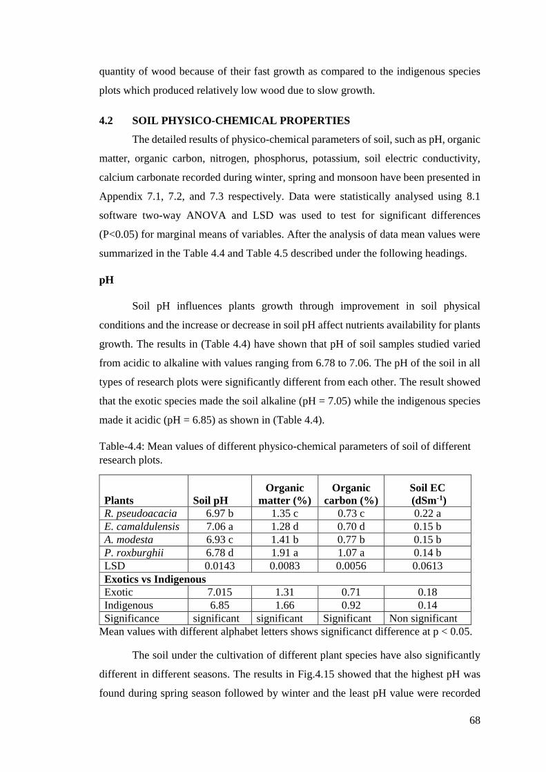
68
quantity of wood because of their fast growth as compared to the indigenous species
plots which produced relatively low wood due to slow growth.
4.2 SOIL PHYSICO-CHEMICAL PROPERTIES
The detailed results of physico-chemical parameters of soil, such as pH, organic
matter, organic carbon, nitrogen, phosphorus, potassium, soil electric conductivity,
calcium carbonate recorded during winter, spring and monsoon have been presented in
Appendix 7.1, 7.2, and 7.3 respectively. Data were statistically analysed using 8.1
software two-way ANOVA and LSD was used to test for significant differences
(P<0.05) for marginal means of variables. After the analysis of data mean values were
summarized in the Table 4.4 and Table 4.5 described under the following headings.
pH
Soil pH influences plants growth through improvement in soil physical
conditions and the increase or decrease in soil pH affect nutrients availability for plants
growth. The results in (Table 4.4) have shown that pH of soil samples studied varied
from acidic to alkaline with values ranging from 6.78 to 7.06. The pH of the soil in all
types of research plots were significantly different from each other. The result showed
that the exotic species made the soil alkaline (pH = 7.05) while the indigenous species
made it acidic (pH = 6.85) as shown in (Table 4.4).
Table-4.4: Mean values of different physico-chemical parameters of soil of different
research plots.
Mean values with different alphabet letters shows significanct difference at p < 0.05.
The soil under the cultivation of different plant species have also significantly
different in different seasons. The results in Fig.4.15 showed that the highest pH was
found during spring season followed by winter and the least pH value were recorded
Plants Soil pH
Organic
matter (%)
Organic
carbon (%)
Soil EC
(dSm-1)
R. pseudoacacia 6.97 b 1.35 c 0.73 c 0.22 a
E. camaldulensis 7.06 a 1.28 d 0.70 d 0.15 b
A. modesta 6.93 c 1.41 b 0.77 b 0.15 b
P. roxburghii 6.78 d 1.91 a 1.07 a 0.14 b
LSD 0.0143 0.0083 0.0056 0.0613
Exotics vs Indigenous
Exotic 7.015 1.31 0.71 0.18
Indigenous 6.85 1.66 0.92 0.14
Significance significant significant Significant Non significant

69
during monsoon in all plots under the cultivation of the different four species. The soil
becomes more acidic under the conditions of warm temperature and excessive rainfall
as weathering of soil takes place rapidly. Leaching of basic cations like, Ca, Mg, K
from the soil profile results in the formation of more stable materials rich in Fe and Al
oxides. This natural process of weathering makes soil more acidic and generally lack
of nutrients (Hue and Uchida, 2000). Shaikh (1996) found that high pH of
Fig.4.15. Showing soil pH of plots of different plants in different seasons.
soil ocuurred in summer and in winter. The present result also revealed that the plots
under cultivation of exotic plants had the high soil pH values while the indigenous
species plots were having low pH values collectively in all seasons. This may be due to
high organic matter contents and undisturbed nature of the indigenous species
plantations as compared to the exotic species plantations. According to Brady and Weil
(2002) the indigenous forest has low pH as compared to the disturbed forest because
organic matter in the form of plant litter, compost, and manure decreased soil pH
through the decomposition process. High amount of humus in the soil of indigenous
plantations is responsible for low soil pH (Dimri et al. 1987). According to De Hann
(1977) low pH occurred due to the accumulation and consequent slow decomposition
of organic matter, which releases acid. Accordind to Bailey et al., 2005 acidification
may lead to depletion of the soil base cations like K+, Mg2+, Ca2+ which arised from
the replacement of the basic cations by Al3+ and H+ ions at the exchange site.
Similarly, Castro-Diez et al. (2011) found that low soil pH limits the growth and
activities of decomposer soil micro-organisms as soil biological activities are reduced
6.96
7.01
6.93
7.05
7.1
7
6.92
6.97
6.89
6.77
6.82
6.746.7
6.8
6.9
7
7.1
Winter Spring Monsoon
Soil
pH
Seasons
Soil pH
R. pseudoacacia
E. camaldulensis
A. modesta
P. roxburghii

70
in acidic soils. As the soil pH in the present study is not as much low as described by
the researchers. Berendse, 1998 reported that at soil pH of below 5.5, soil trace nutrients
like Manganese (Mn) and Aluminium (Al) availability increase to levels that become
toxic for most plant growth. Further, soil nutrients such as phosphorus and nitrogen
tend to form insoluble compounds with Al and Fe in acidic soils, become adsorbed and
therefore, made inaccessible for plant uptake.
The result of this study was supported by Robertson and Vitousek (1981) and
Adams and Sidle (1987) who reported low pH in indigenous forest soils as compared
to plantation forest soils. According to Leskiw (1998) the forest soils should be slightly
acidic to keep balance for nutrient supply. Semwal et al. (2009) found that the pH values
were highly acidic in the indigenous forest as compare to disturbed forest. Contrasting
results were found by Rhoades & Binkley (1996) Cao et al. (2010) and Alemie (2009)
who reported low soil pH in exotic Eucalyptus spp. plantations as compared to native
species plantations. Aweto and Moleele (2005) claimed that Eucalyptus species
immobilized soil exchangeable bases, especially calcium leading to low soil pH.
Organic matter (OM)
Organic matter influences physical and chemical properties of soil and
determines the cation exchange capacity of the soil. The formation of organic matter
occurs as a result of decomposition of plant tissues and digestion of microorganisms.
Soil humus is the result of organic compounds like resistant compounds of high plant
origin such as oil, fats waxes, lignin and new compounds such as polysaccharides and
polyuronides. Soil organic matter in soil speed up the weathering process in the soil and
results in increasing the availability of nutrient ion species. Potassium and phosphorus
in soil in the available form is due to the availability of soil organic matter (Brandy,
1974).
It is clear from the data (Table 4.4) that organic matter contents (%) varied from
1.28% to 1.91% in the soil samples of different research plots of the study area. Mean
values were significantly different from each other. The greatest mean value of 1.91%
was recorded for Pinus roxburghii plots, followed by A. modesta, R. pseudoacacia plots
with the values of 1.41%, 1.35% respectively and the lowest value of 1.28% was
recorded for E. camaldulensis plots soils. Regarding the comparison between
indigenous and exotic, the result showed that maximum organic matter 1.66% was

71
found for indigenous species plots while the lowest organic matter 1.31% were found
for exotic species plots of the study area.
The organic matter content also significantly fluctuated during different
seasons. The result showed that maximum organic matter was recorded during the
monsoon season followed by winter season and the lowest during the spring season, all
the four species plots follow the same patteren as shown in (Fig. 4.16). Organic matter
recorded from all of the four plots during three different seasons showed the following
pattern P. roxburghii > A. modesta > R. pseudoacacia > E. camaldulensis.
Fig. 4.16. Showing organic matter (%) in plots of different plants in different
seasons.
Seasonal variations in soil organic matter have been extensively studied by (Angers,
1992; Leinweber et al.,1994; Powlson et al. 2003; Hendrix, 1997; Kieft et al., 1998;
Knops and Tilman, 2000 and Dabek-Szreniawska and Balashov, 2007). The
accumulation of organic matter in soil is strongly influenced by temperature and by the
availability of oxygen, since the rate of biodegradation decreses with decrease in
temperature; organic matter does not degrade rapidly in colder climates and tend to
build up in soil (Manalian, 1994).
The results showed that the maximum percentage of OM was observed in the
plots of indigenous species plantations and minimum in exotic species plantations. In
all type of plots of species maximum organic matter percentage was recorded in
1.27 1.17
1.57
1.22 1.12
1.51.34 1…
1.64
1…
1.75
2.15
1
1.5
2
2.5
Winter Spring Monsoon
Org
an
ic m
att
er (
%)
Seasons
Organic matter
R. pseudoacacia
E. camaldulensis
A. modesta
P. roxburghii

72
monsoon season followed by winter and minimum during spring season. Declining
trend during the spring season may be due to the decrease in organic matters contents
with increase in temperature and decomposition rates became doubles with every 10 oC
increase in the temperature (Schlesinger, 1997; Hartel, 2005; Kirschbaum, 1995;
Albrecht and Rasmussen, 1995). The greater amount of organic matter in the
indigenous plots may be due to production and returns of large amount of litter (Sevgi
and Tecimen, 2008). The release of nutrients from litter decomposition is a natural
process in the internal biogeochemical cycle of an ecosystem, and decomposers recycle
a large amount of carbon that was bounded in the plant or tree to the atmosphere. The
results also revealed that soils in the indigenous plots had the maximum content of
organic matter in all the seasons and the minimum was observed under exotic plots in
all the seasons. This may be due to large amount of litter produced in indigenous species
plots as compared to exotics species plots therefore, accumulation of organic matter
was higher.
According to Lima et al. (2008) considerable changes in soil organic matter
(SOM) occurred when native vegetation was replaced with exotic Eucalyptus spp.
plantations in Brazil. Similarly, Bhatti et al. (2002) found that 83 % in the surface soil
and 94 % in the sub-soil of soil samples in Pakistan were low (< 1 %) in organic matter
under exotic Eucalyptus spp. plantation soils. Jan et al. (1996) also found great changes
in organic matter in Eucalyptus spp. plantation soils relative to Shorea robusta natural
forest soil in Uttar Pradesh, Bangladesh. Result of a study carried out on the effect of
Eucalyptus camaldulensis plantations on soil properties and soil fertility in D. I. Khan
District in Pakistan, showed that the organic matter content in the surface soil at 0-15
cm depth ranged from 0.38 to 1.10 %., which were low according to the established
criteria (Baber et al., 2006). The level of Organic matter contents is considered low if
it is less than 4 %, medium if it is between 4 % and 8 %, and high if it is above 8 %
(University of Connecticut, Cooperative Extension System, 2003). Chen et al. (2013)
found that during deforestation of native vegetation and establishment of exotic
Eucalyptus spp. plantation, soil macro-aggregates were disrupted and exposed to
microbial breakdown, as a result of organic matter being lost from soil. Zhang et al.
(2012) add that lower organic matter inputs are provided to the soil since young
Eucalyptus spp. stands may provide a low amount of inputs of plant residues to the soil.

73
Organic Carbon
The presence of organic carbon in soil regulates the growth of microorganisms
and makes the system more dynamic. The result revealed in Table 4.4, appendix-10
showed that OC contents (%) calculated from the soil samples of the research plots
during three different seasons showed variations from 0.70% to 1.07%. The result
showed that OC contents in percent in all types of plots of different species were
significantly different from each other. Comparison between exotic and indigenous
species plots showed that more organic carbon (0.92%), was recorded for indigenous
species plots while lower (0.71%) was recorded for exotic species plots.
Fig. 4.17. Showing soil organic carbon (%) in plots of different plants in different
seasons.
The OC percentage in the soil of plots of different species fluctuates during
different seasons. The result showed that maximum OC was recorded during the
monsoon season followed by winter season and the lowest during the spring season
(Fig.4.17). Organic Carbon recorded from all of the four plots during three different
seasons showed the following pattern P. roxburghii > A. modesta > R. pseudoacacia >
E. camaldulensis.
The results revealed in Fig. 4.17 shows that the organic carbon content were
maximum in monsoon followed by winter and minimum in spring. The decrease in the
soil OC in spring may be due to the increase in temperature and high decomposition
0.74
0.64
0.82
0.7
0.6
0.780.78
0.68
0.86
1.07
0.97
1.15
0.4
0.6
0.8
1
1.2
Winter Spring Monsoon
Org
an
ic c
arb
on
(%
)
Seasons
Organic carbon
R. pseudoacacia
E. camaldulensis
A. modesta
P. roxburghii

74
rate (Kirschbaum, 1995; Albrecht and Rasmussen, 1995). Maximum OC in the
indigenous plots may be due to the high amount of litter in soil (Sevgi and Tecimen,
2008). Nutrients released through the process of decomposition by decomposers and
soil carbon was recycled in large quantity that was bounded in the plant or tree to the
atmosphere.
The results also revealed that soils in the indigenous plots had the maximum
content of organic carbon in all the seasons and the minimum was observed under
exotic plots in all the seasons. This may be due to large amount of litter produced in
indigenous plots of species as compared to exotic species plots where the
decomposition rate of litter was comparatively slow therefore, accumulation of organ
carbon was higher in indigenous as compared to exotics.
Similarly, study carried out by Bernhard-Reversat (1998) found that the organic
carbon concentration in the 0–10 cm depth of native Acacia seyal woodland in Keur
Maktar, Senegal was twice that in a corresponding layer of soil under Eucalyptus spp.
plantation. Cortez et al. (2014), reported that organic C decreased in the first year of
the conversion of native forest to exotic plantations in Brazil. Hou (2006) further
suggested that exotic species of Eucalyptus have a high growth rate and C fixation
potential; therefore, part of the assimilated C is transported to the soil through litter fall
and rhizo- deposits, and hence the potential of increasing soil organic content with time
(Lima et al., 2006). Therefore, it is likely that the changes in soil chemical properties,
particularly in SOM, differ after several exotic plantation rotations, varying with the
soil type and dominant climate conditions (Leite et al., 2010).
Soil Electric conductivity
It is evident from the table 4.4 that the highest value 0.22 dSm-1 was recorded
for R. pseudoacacia and the lowest value 0.14 dSm-1 was recorded for P. roxburghii
species plots. The result showed that soil EC among different plots of plant were not
different significantly from each other and the exotic and indigenous plots of plants
were also not significantly different. This may be due to the same soil texture i.e. sandy
loam of soil in all plots of plants due to which the soil EC were not significantly
different from each other.
Soil EC is a measurement that reflects crop productivity, soil texture, cation
exchange capacity (CEC), drainage conditions, organic matter level, salinity and

75
subsoil characteristics. Sands have a low conductivity, silts have a medium
conductivity, and clays have a high conductivity. Soil EC is mainly correlated to the
presence of soluble salts in the soil (Ali and Rub, 2017). In present study, the soluble
salts may drain out from the root zone due to the sandy loam texture of all the plots soil.
Sandy loame texture are always low in EC (McKenzie and Jacquier, 1997).
Fig. 4.18. Showing soil electrical conductivity of plots of different plants in
different seasons.
Among the different seasons the EC fluctuates (Fig.4.18) but not significantly
(Table 4.4). Among the different plants species R. pseudoacacia plots with high E.C
was recorded than the other three species. This may be due to the low absorption of
soluble salts in R. pseudoacacia plots or more sensitivity of the species to salinity than
the rest of the species. While the other three species may have the ability to absorb soil
solutions of relatively high soluble salts (Fig.4.18).
Among the different seasons as in the spring the temperature goes up the soil
become relatively dry, therefore the presence of soluble salts may be related to soil
texture and in monsoon and winter were wet seasons therefore the soluble salts were
drained out as the soil texture is loos.
0.24
0.2 0.22
0.15
0.19
0.13
0.14
0.18
0.120.13
0.17
0.110.1
0.12
0.14
0.16
0.18
0.2
0.22
0.24
Winter Spring Monsoon
Soil
EC
(d
Sm
-1)
Seasons
Soil Electrical Conductivity
R. pseudoacacia
E. camaldulensis
A. modesta
P. roxburghii

76
Nitrogen
The result revealed in Table 4.5 that soil total nitrogen among the plots of
different species varied from 0.110% to 0.077%. Total nitrogen in percent recorded
from different plots of species were significantly different from each other. The highest
value (0.0865%) was recorded for indigenous species plots while the lowest value
(0.07551%) was recorded for exotic species plots.
Table-4.5: Means showing nutritional status of different species plots.
Mean values with different alphabet letters shows significanct difference at p < 0.05.
Fig. 4.19. Showing soil total nitrogen in percent of plots of different plants in
different seasons.
The result in Fig. 4.19. showed that Soil N contents were recorded highest
during the monsoon season followed by winter season and the lowest was recorded
0.07
0.05
0.10.1
0.08
0.13
0
0.02
0.04
0.06
0.08
0.1
0.12
0.14
Winter Spring Monsoon
Tota
l n
itro
gen
(%
)
Seasons
Total nitrogen
R. pseudoacacia, E. camaldulensis and A. modesta P. roxburghii
Plants
Total
Nitrogen
(%)
Phosphorus
(ppm)
Potassium
(ppm)
Calcium
carbonate
(mmole/meter)
R. pseudoacacia 0.077 c 7.4 c 90.3 c 4.8 c
E.camaldulensis 0.074 d 7.1 d 86.3 d 5.7 a
A. modesta 0.081 b 7.89 b 95.25 b 5.2 b
P. roxburghii 0.110 a 10.8 a 130.3 a 3.4 d
LSD 0.00053 0.053 0.644 0.093
Exotics vs Indigenous
Exotic 0.075 7.25 88.3 5.2
Indigenous 0.086 9.34 112.7 4.3
Significance Significant significant significant Significant

77
during spring season in all types of plots of plants. As all the three species (A. modesta,
R. pseudoacacia and E. camaldulensis plots) have the same recorded values in each and
every season, therefore the graph in Fig. 4.19. shows single line for the three species.
Whereas P. roxburghii plots were having highest N in all seasons as compared to the
other three species.
Among the different seasons the total nitrogen in the soil was less in spring as
compared to the monsoon and winter seasons because the spring season is active season
for most of the plants and most of the N from the soil were utilized due to which the
concentration of N in the soil become low and the soil was depleted in spring season.
The increased nitrogen contents during the rainy monsoon season could be best
explained by the possible activity of nitrogen fixing microbes. Evidence exists to show
that increased biological nitrogen fixation along with increased mineralization rates
occur during the rainy season, which resulted in increased nitrogen content at this time
(Bergeron et al. 2002). Higher values of total nitrogen in the soil profile during rainy
season reflects blue green algae fixation, rain water input and higher rate of release of
mineral nitrogen through microbial decomposition (Birch, 1958 and Choudhri and
Sharma, 1975). Singh and Singh (2006) reported that during dry periods, plant uptake
of nutrients is greatly reduced and the N-mineralization and nitrification are either
immobilized in microbial biomass or accumulate in the soil as inorganic nitrogen and
the minimum was observed in spring season. The results showed that during winter
season with little or no rain, there is no leaching of nutrients from the soil which results
in the accumulation of high nutrients in winter after monsoon season.
The rate of nitrogen release to plant growth is rapid during the warm growing
season and slow during the winter months (Manahan, 1994). According to FAO (2011)
soil total N and available P decreased as a result of reforestation with exotic plantations.
Similarly, study carried out by Leite et al. (2010) concluded that large nutrient amounts
are exported when exotic Eucalyptus spp. plantation are harvested, causing a reduction
in the soil nutrients content such as total N and available P. Jagger and Pender (2000)
found that fast growing non-leguminous exotic species are not recommended for
intercropping with annual crops. Tererai et al. (2014) found that reduction in soil total
N occured with an increase in exotic Eucalyptus camaldulensis cover compared to the
site not covered by the Eucalyptus spp. in South Africa. Alemie (2009) also found that
concentration of soil TN decreased under plantations of exotic species in Ethiopia.
Nitrogen concentration in soils is associated with the rate of decomposition of the plant

78
material (Demessie et al., 2012). Aweto and Moleele (2005) Baber et al. (2006) Cao et
al. (2010) and Demessie et al. (2012) found that Eucalyptus spp. produce litter with
low nutrient concentrations, which decomposes slowly to release low concentrations of
nutrients.
Phosphorus (P)
It is evident from the table 4.5 that the Phosphorus values (ppm) recorded in
different plots of species varied in a range of 7.1 ppm to 10.8 ppm. The greatest mean
value 10.8 ppm was recorded for Pinus roxburghii plots while the lowest value 7.1 ppm
was recorded for E. camaldulensis plots. The result showed that the concentration of
soil phosphorus contents was greater in indigenous plots (9.34%) as compared to exotic
plots (7.25%).
Fig. 4.20. Showing soil available phosphorus (ppm) of plots of different plants in
different seasons.
The phosphorus level also fluctuated significantly during different seasons. The
results in Fig. 4.20 showed that maximum phosphorus occurred during monsoon season
followed by winter season and the lowest were recorded during spring season in all
types of plots of plants. Mean values of phosphorus recorded from all of the four plots
during three different seasons showed the following pattern P. roxburghii > A. modesta
> R. pseudoacacia > E. camaldulensis.
7.42
5.67
9.37
7.08 5.33
9.037.82
6.07
9.77
10.74
8.99
12.69
5
6
7
8
9
10
11
12
13
Winter Spring Monsoon
Ph
osp
horu
s (p
pm
)
Seasons
Phosphorus
R. pseudoacacia
E. camaldulensis
A. modesta
P. roxburghii

79
The high level of phosphorous recorded in indigenous plots of species as
compared to the exotic plots may be due to the production and returns of large amount
of litter and the release of nutrients from litter decomposition (Sevgi and Tecimen,
2008).
Phosphorus is an important component of plants mostly available in
orthophosphate form at the neutral soil pH. The inorganic phosphorus in soil depends
on soil pH, soluble iron, aluminium and manganese, the presence of iron, aluminium
and manganese containing minerals, calcium minerals, amount and decomposition of
organic matters and activities of microorganisms (Manahan, 1994). The decrease in the
soil phosphorus level during the springs season was due to the active season of plants
growth and most of the available phosphorus in the soil was depleted by plant uptake.
While maximum amount of phosphorous during monsoon followed by winter might be
due to more accumulation of minerals in monsoon and winter seasons. According to
Ashraf et al. (2012) soil with more leaching contains less amount of phosphorus in
comparison to the soil with less leaching. The result of the present study is similar with
the study carried out by Fith and Nelson (1956) and Keogh et al. (1972) by concluding
that when soil levels for phosphorus and percent organic matter are high, the amount of
potential seasonal variation of phosphorus values tends to increase. Semwal et al.
(2009) reported that the available phosphorus occurred more in winter season due to
more accumulation of minerals takes place in winter season. Miller and Donahuer
(2001) reported that the soil with high organic matter content have better supplies of
organic phosphate for plant uptake than have the soils with low organic content. Gupta
and Sharma (2008) also reported that carbon and phosphorus were positively correlated
because all these attributes were intimately linked with soil humus.
The result of this research is in accordance with the studies conducted by FAO
(2011) Leite et al. (2010) Jagger and Pender, (2000) pointed out that soil total N and
available P decreased as a result of reforestation with exotic plantation and emphasized
not to recommend the fast growing non-leguminous Eucalyptus spp. for intercropping
with annual crops. Similarly, Aweto and Moleele (2005) found that soil available
phosphorus was relatively low in soil under Eucalyptus spp. plantation due to the long-
term immobilization in the plantation standing biomass. In Australia, Polglase et al.
(1992) found that the concentration of soil available phosphorus in the topsoil (0–5 cm

80
depth) under exotic plantation declined from an initial concentration of 34 to 2.3 µg g−1
of soil after 16 years. Alemie (2009) further reported that soil available phosphorus
concentration in Eucalyptus spp. plantation within 2 cm depth of soil was in the very
low range (< 5 mg kg-1) in Ethiopia.
Potassium
It is clear from the Table 4.5 that the mean values of K recorded from different
plots of species were significantly different from each other and comparison between
indigenous and exotic species plots showed that more K (112.7 ppm) was recorded for
indigenous species plots while low K level (88.3 ppm) was recorded for exotic species
plots.
Fig. 4.21. Showing Soil potassium (ppm) of different plants in different seasons.
The level of K fluctuated significantly during different seasons. The result
revealed in Fig. 4.21 that highest level of K was found during monsoon season followed
by winter season and the lowest during spring season in soil of all species plots. Mean
values of K recorded from all of the four plots during three different seasons showed
the following pattern P. roxburghii > A. modesta > R. pseudoacacia > E. camaldulensis.
The greater availability of potassium observed in the soil of indigenous species
plots as compared to exotic species plots may be due to the presence of dense vegetation
in indigenous plots which reduced loss in soil micro and macro nutrients essential for
plants growth and energy fluxes as compared to the exotic plots where there were less
89.0482.04
100.04
84.9877.98
95.9893.92
86.92
104.92
128.98
121.98
139.98
70
80
90
100
110
120
130
140
Winter Spring Monsoon
Pota
ssiu
m (
pp
m)
Seasons
Potassium
R. pseudoacacia
E. camaldulensis
A. modesta
P. roxburghii

81
vegetations (Iwara et al., 2011). The decreased in the level of soil potassium during
springs season might be due to the high uptake rate during active season of plants
growth and most of the available potassium in the soil was depleted as a result of plants
uptake. While the maximum amount of phosphorous was during the monsoon followed
by winter this might be due to more accumulation of minerals in monsoon and winter
seasons. It was observed from the above results that the greater the organic matter, the
larger is the accumulation of minerals in the soil. This was also reported by Chauhan
(2001) by finding a positive corelationship between organic matter and available
potassium and that with the increase in organic matter tends to increase the
accumulation of available potassium in the soil. Potassium values generally increase
during the winter months because of shifts in soil equilibrium conditions due to freezing
and thawing actions releasing fixed potassium from non exchangeable forms,
depending upon the type of clay minerals present (Fine et al., 1940 and Keogh, et al.
1972).
The result in this study is supported by studies of Nwoboshi (1972) and Chijioke
(1978) in which they reported low concentration of potassium in the soil of exotic tree
species plantations as compared to the indigenous tree species. This low concentration
of potassium showed that exotic tree species absorb more K as compared to the
indigenous tree species.
Calcium carbonate
It is evident from the Table 4.5 that the calcium carbonate contents in different
species plots varied significantly from each other and higher calcium carbonate contents
(5.25 mmole/meter) was found in exotic species plots while lowest (4.3 mmole/meter)
in indigenous species plots.
The results in Fig. 4.22 showed that highest calcium carbonate was found during
the spring season followed by the winter season and the lowest was recorded during the
monsoon season in all plots of different plants. Mean values of calcium carbonate
recorded from all of the four plots during three different seasons showed the following
pattern E. camaldulensis. > A. modesta > R. pseudoacacia > P. roxburghii.

82
Fig. 4.22. Showing Calcium carbonate (mmole /meter) of plots of different
plants in different seasons.
According to Curtin and Smeller (1995) the greater amount of lime in exotic plots
of plants may be due to high pH in exotic plots and low lime contents in indigenous
plots of plants may be due to low soil pH in indigenous plots. The result showed that
highest calcium carbonate was found during the spring season and lowest during the
monsoon season in all plots of different species. This may be due to the increased
leaching effect during the rainy monsoon season and winter season while the
concentration of lime on the surface increase during hot and dry season.
Lime contents affect physically the decomposition of soil organic matter,
synthesis of humus and the stimulation of nitrogen fixing bacteria and chemically by
decreasing the concentration of hydrogen ions, increase in the concentration of
hydroxyl ion, decline in the solubility of iron, aluminium and manganese, increase in
the availability of phosphate and molybdates, increase in the ion exchange of calcium,
magnesium and the availability of potassium while biologically by accelerating the
activity of heterotropic soil organism which not only favours, the formation of humus
but also encourages the elimination of certain organic intermediate product that might
be toxic to plants (Brandy, 1974).
4.35
6.65
3.65
5.17
7.47
4.47
4.67
6.97
3.97
2.9
5.2
2.22
3
4
5
6
7
8
Winter Spring Monsoon
Calc
ium
carb
on
ate
(m
mole
/met
er)
Seasons
Calcium carbonate
R. pseudoacacia
E. camaldulensis
A. modesta
P. roxburghii

83
4.3 SOCIO-ECONOMIC IMPACTS OF THE MONOCULTURE OF
EXOTIC TREE SPECIES
Plantations of fast growing species have increased over the last two decades
which helps in uplifting the socio-economic condition of the local inhabitants by
employment generation in plantation, nurseries and business in timbers. Plantations of
Eucalyptus camaldulensis and R. pseudoacacia are found in the study area.
Agriculture land is mostly used for woodlot plantation. Among all other exotic
species available in Pakistan, Eucalyptus camaldulensis was found to be highly
adaptable and fast growing tree species to withstand even degraded site conditions and
in a wide range of soils under different conditions (Kamara and Maghembe, 1994; NAS,
1980; Duguma and Tonye, 1994 and Akkasaeng et al., 1989). Eucalyptus and Robinia
pseudoacacia proved successful for afforestation, reforestation and agroforestry
programs in Pakistan. Exotic tree species put pressure on the environment and
ultimately directly and indirectly have affect at different levels and there was a need to
undertake a detailed investigation. The decisions to plant exotic tree species are based
primarily on the potential economic benefits and short term gains without considering
long term gains and sustainability of environment.
Mostly poor communities rely on short-term economic gains from exotic
species and do not know the complexity of planting such species. They are unaware of
the negative impacts of monoculture of exotic species on natural ecosystem and
biodiversity that are affecting their long term economic gains. Keeping these views in
mind, the socio-economic impacts of monoculture of exotic tree species in District
Malakand were assessed to determine how monoculture plantations of exotic tree
species are affecting the local economy and every-day life of the local people.
The research area baseline information on the exotic tree growers and their
socio-economic impacts were collected. The cost and benefits of raising woodlot
plantations were calculated. The information was collected through a comprehensive
questionnaire survey. The results of the information gathered has been described under
the following headings.
4.3.1 Basic Information of the tree growers
The results of the survey showed that all household heads who were growing
trees were male and they were all married. The respondents who were growing trees

84
in their land were on average age of 50 years old with a minimum age of 32 years and
a maximum age of 75 years. 90% of the respondents were literate while 10% were
illiterate.
Education
Among the total 30 tree growers, 10% i.e. only 3 respondents were found to be
illiterate while 27 (90%) of the them were literate, of which 8 (27%) were educated up
to primary level, 14 (47%) of the respondents were educated up to secondary school
level, 2 (7%) were educated to higher secondary level while, 2 (7%) were graduate and
only 1(2%) of the respondents were educated to postgraduate level.
Occupation
The occupation of most of the respondents who were growing tree were
agriculture. About 21 (70%) of the respondents had an occupation of agriculture, 6
(20%) of the respondents were doing their own business and 2 (7%) of the respondents
were social workers while only 1 (3%) of the respondent was a teacher.
Land Use Pattern
In the research area lands were utilized mostly for farming, housing and forestry
(tree cultivation) purposes. The average land holding size collectively of the all the
respondents were 0.88 ha, of which 18%, 52% and 30% were used for homesteads,
agricultural and tree plantation purposes respectively. The average land size for each
homestead was 0.16 ha with a minimum size of 0.07 ha to maximum size of 0.52 ha. In
case of land holdings, respondents were divided into three land holdings classes such
as respondents having more than 0.25 ha of land, classified as large farmer; less than
0.25 ha but greater than 0.15 ha, classified as medium farmer; and less than 0.15 ha
were classified as small farmer. Out of 30 respondents, only 9 (30%) households had
above 0.25 ha landholding size used for tree growing. While, 13 (43%) of the
respondents had landholding size between 1.5 hac to 2.5 hac used for growing trees and
only 8 (27%) of the respondents were landholding size below 1.5 hac for growing trees
on their lands (Table-4.6).

85
Table- 4.6. Basic information of woodlot tree grower of District Malakand.
Respondent
ID
Age Education Occupation Plot species Farmer
category
Homestead
land (hac)
Agriculture
land (hac)
Land with
trees (hac)
Total
land
(hac)
1 37 SSC Business Eucalyptus Large 0.2 0.57 0.33 1.1
2 40 SSC Agriculture Eucalyptus Large 0.27 0.78 0.45 1.5
3 45 HSSC Business Eucalyptus Large 0.52 1.51 0.87 2.9
4 51 SSC Business Eucalyptus Medium 0.1 0.29 0.17 0.56
5 70 SSC Business Eucalyptus Small 0.08 0.24 0.14 0.46
6 62 FIVE Agriculture Eucalyptus Medium 0.1 0.28 0.16 0.53
7 47 SSC Agriculture Eucalyptus Medium 0.12 0.33 0.19 0.64
8 38 BA UC Member Robinia Large 0.5 1.46 0.84 2.8
9 66 SSC Agriculture Eucalyptus Medium 0.1 0.29 0.17 0.55
10 46 NIL Agriculture Eucalyptus Large 0.3 0.86 0.5 1.66
11 42 FIVE Agriculture Eucalyptus Small 0.07 0.19 0.11 0.37
12 54 FIVE Agriculture Eucalyptus Medium 0.14 0.4 0.23 0.76
13 67 NIL Agriculture Eucalyptus Small 0.07 0.2 0.11 0.38
14 56 SSC Business Eucalyptus Medium 0.12 0.33 0.19 0.64
15 47 SSC Agriculture Eucalyptus Medium 0.13 0.37 0.21 0.71
16 60 FIVE Agriculture Robinia Small 0.08 0.24 0.14 0.47
17 44 MA Teacher Eucalyptus Large 0.34 0.99 0.57 1.9
18 48 BA Business Eucalyptus Medium 0.14 0.41 0.23 0.78
19 36 SSC Agriculture Eucalyptus Large 0.22 0.62 0.36 1.2
20 64 SSC Agriculture Eucalyptus Large 0.2 0.57 0.33 1.1
21 50 FIVE Agriculture Eucalyptus Large 0.16 0.46 0.26 0.88
22 36 SSC Agriculture Eucalyptus Medium 0.11 0.32 0.19 0.62

86
23 49 FIVE Agriculture Eucalyptus Small 0.07 0.2 0.12 0.39
24 58 FIVE Agriculture Robinia small 0.08 0.22 0.13 0.42
25 67 SSC Agriculture Eucalyptus small 0.08 0.23 0.13 0.44
26 32 HSSC UC Member Robinia Medium 0.12 0.35 0.2 0.67
27 49 SSC Agriculture Eucalyptus Medium 0.09 0.25 0.15 0.49
28 52 FIVE Agriculture Eucalyptus Medium 0.1 0.28 0.16 0.54
29 75 NIL Agriculture Eucalyptus Small 0.08 0.24 0.14 0.46
30 41 SSC Agriculture Eucalyptus Medium 0.09 0.27 0.15 0.51
87
4.3.2 CHARACTERISTICS AND FACTORS OF WOODLOT PLANTATION
OF EXOTIC TREE SPECIES
In the research areas, woodlot plantations of the fast growing exotic tree species
of Eucalyptus camaldulensis and Robinia pseudoacacia were carried out. Among these
Eucalyptus camaldulensis occupied the major portion. A sufficient number of woodlots
of exotic species of different ages were found in the private land of the study areas,
among them 30 similar kinds of woodlot plots were selected based on the objectives of
the present research. Questionnaire survey revealed that, among the 30 woodlot tree
growers (respondents), 80% and 20% tree growers collected seedlings from the local
nurseries and local market respectively.
The tree growers planted seedlings that were 1-year-old and on average 0.79 m
in height. The spacing in plantations was different among different woodlot plantations.
The average number of saplings/seedlings planted initially per hectare was recorded as
2226 with a maximum of 5850 and minimum 740 and these variations in number of
seedlings were mainly due to the spacing reported by the respondents.
The average age of the privately owned woodlot of exotic trees was 4 years, and
on average, one hectare of woodlot plots was comprised 2226 trees, of which the
average tree height and DBH were 6.6 m and 10.3 cm respectively (Table 4.7).
When the respondents were asked about the previous land use pattern, most of
the respondents i.e. 16 (53%) of the respondents had previously used the land for
agricultural purposes, 4 (14%) of the respondents raised trees on barren land, while 10
(33%) raised trees on land previously occupied by scrub forest of Acacia modesta and
Dodonea viscosa.

88
Table-4.7. Characteristics of different woodlot plantation raised by the tree growers in District Malaakand.
Respondent
ID
Plot species Avg.
height of
seedlings
(m)
Avg. age
of
seedlings
Plantation
year
Age
of
trees
(yrs)
Trees/hac
while
survey
Avg.
height
(m) of
trees
Avg. DBH
(cm) of
trees
Tree
growth
pattern
Previous land
use
1 Eucalyptus 0.59 1 2014 4 3596 7.68 10.2 Fast Agriculture
2 Eucalyptus 0.61 1 2015 3 2807 5.78 8.8 Fast Agriculture
3 Eucalyptus 0.63 1 2012 6 5620 9.15 14.12 Fast Agriculture
4 Eucalyptus 0.66 1 2011 7 1930 10.88 17.01 Fast Agriculture
5 Eucalyptus 0.69 1 2012 6 880 8.78 16.91 Fast Agriculture
6 Eucalyptus 0.63 1 2014 4 1882 6.15 11.8 Fast Agriculture
7 Eucalyptus 0.61 1 2015 3 1199 5.88 8.12 Fast Agriculture
8 Robinia 1.52 1 2014 4 3413 5.19 8.81 Medium Agriculture
9 Eucalyptus 0.59 1 2015 3 1980 5.97 8.8 Fast Agriculture
10 Eucalyptus 0.61 1 2015 3 2963 5.78 8.12 Fast Agriculture
11 Eucalyptus 0.63 1 2015 3 640 5.15 8.01 Fast Barren land
12 Eucalyptus 0.66 1 2015 3 2519 5.88 8.2 Fast Barren land
13 Eucalyptus 0.69 1 2014 4 650 7.78 10.8 Fast Barren land
14 Eucalyptus 0.63 1 2015 3 1188 5.15 8.12 Fast Barren land
15 Eucalyptus 0.61 1 2014 4 1990 7.88 11.01 Fast Agriculture
16 Robinia 1.52 1 2015 3 851 4.19 6.92 Medium Agriculture
17 Eucalyptus 0.61 1 2015 3 3423 5.78 8.12 Fast Agriculture
18 Eucalyptus 0.63 1 2015 3 893 5.15 8.8 Fast Scrub forest
19 Eucalyptus 0.66 1 2012 6 3884 8.88 15.12 Fast Scrub forest
20 Eucalyptus 0.69 1 2014 4 3543 7.78 10.01 Fast Scrub forest
21 Eucalyptus 0.63 1 2015 3 2908 5.15 8.91 Fast Scrub forest

89
22 Robinia 1.52 1 2012 6 1085 6.71 13.78 Medium Agriculture
23 Eucalyptus 0.66 1 2014 4 1237 7.78 11.12 Fast Scrub forest
24 Robinia 1.52 1 2015 3 780 4.83 6.92 Medium Agriculture
25 Eucalyptus 0.66 1 2014 4 1467 7.78 10.12 Fast Scrub forest
26 Robinia 1.52 1 2015 3 1278 4.19 6.92 Medium Agriculture
27 Eucalyptus 0.63 1 2014 4 1524 7.78 11.12 Fast Scrub forest
28 Eucalyptus 0.66 1 2015 3 1698 5.15 8.8 Fast Scrub forest
29 Eucalyptus 0.69 1 2012 6 1568 8.88 16.12 Fast Scrub forest
30 Eucalyptus 0.63 1 2015 3 1598 5.15 8.91 Fast Scrub forest

90
4.3.3 EXPENDITURE FOR WOODLOT PLANTATION OF EXOTIC TREE
SPECIES
Woodlot plantation and maintenance is a labour intensive work. Information
collected from the tree growers showed that, out of total average expenditure, 6.1% was
used for seedlings purchase. 61.9% of the average expenditure per hac was used for the
labour and watch and wards. Thus 68% of the total average cost on raising one-hectare
plantation was used for the purchase of seedlings and labour and watcher collectively.
While the rest of the cost incurred on stacking, transport, fencing, thinning and pruning.
About 3% of the cost were used for the transportation of seedlings from the nursery to
the plantation sites While for stacking fencing, thinning and pruning 4%, 6%, 6% and
4% were used. 9% of the cost was used for the purpose of watering.
Expenditure of tree grower for raising one hectare of private woodlot plantations
in District Malakand was summarised in Table 4.8.

91
Table-4.8. Expenditure of tree growers for raising one-hectare woodlot plantations in District Malakand.
Respondent
ID
Purchase of
seedlings (Rs.)
Transport
(Rs.)
Labor/watcher
(Rs.)
Fencing
(Rs.)
Stacking
(Rs.)
Watering
(Rs.)
Thinning
(Rs.)
Pruning
(Rs.)
Total projected
expenditure/cost
up to rotation (Rs.)
1 15780 8403 173379 16806 11204 25209 16806 11204 278789
2 12104 6445 132990 12891 8594 19336 12891 8594 213844
3 23400 12461 257102 24921 16614 37382 24921 16614 413414
4 8128 4328 89304 8656 5771 12984 8656 5771 143599
5 3764 2004 41356 4009 2672 6013 4009 2672 66500
6 7652 4075 84074 8149 5433 12224 8149 5433 135190
7 5112 2722 56167 5444 3630 8166 5444 3630 90315
8 25305 8134 167826 16268 10845 24401 16268 10845 279891
9 8128 4328 89304 8656 5771 12984 8656 5771 143599
10 13448 7161 147757 14322 9548 21483 14322 9548 237589
11 2960 1576 32522 3152 2102 4729 3152 2102 52295
12 10996 5855 120816 11711 7807 17566 11711 7807 194269
13 2960 1576 32522 3152 2102 4729 3152 2102 52295
14 5112 2722 56167 5444 3630 8166 5444 3630 90315
15 10040 5346 110312 10693 7128 16039 10693 7128 177379
16 6587 2117 43686 4235 2823 6352 4235 2823 72857
17 15332 8164 168457 16329 10886 24493 16329 10886 270874
18 3960 2109 43510 4217 2812 6326 4217 2812 69962
19 17212 9165 189113 18331 12221 27496 18331 12221 304089
20 15780 8403 173379 16806 11204 25209 16806 11204 278789
21 12432 6620 136593 13240 8827 19860 13240 8827 219639
22 8946 2876 59331 5751 3834 8627 5751 3834 98949
23 5736 3054 63023 6109 4073 9163 6109 4073 101339
24 6118 1967 40575 3933 2622 5900 3933 2622 67669

92
25 6216 3310 68297 6620 4413 9930 6620 4413 109820
26 9415 3026 62442 6053 4035 9079 6053 4035 104137
27 7172 3819 78801 7638 5092 11457 7638 5092 126710
28 7652 4075 84074 8149 5433 12224 8149 5433 135190
29 6696 3566 73571 7131 4754 10697 7131 4754 118300
30 7172 3819 78801 7638 5092 11457 7638 5092 126710
Average 9711 4774 98508 9548 6366 14323 9548 6366 159144
Percent 6.1% 3% 61.9% 6% 4% 9% 6% 4% 100%

93
4.3.4 BENEFIT COST ANALYSIS ON WOODLOTS OF EXOTIC TREE
SPECIES
The results of benefit-cost analysis on the woodlots have been presented in
Table 4.10. The results showed that on average, a tree grower spent Rs. 159144 for
woodlot plantation in one hectare of land (Table 4.8). On the other hand, they were
expecting to sale the timber/wood for Rs. 2049478 and to get the, expected net profit
of Rs.1956206 over a ten-year rotation period (Table 4.10).
Net Present Value, Internal Rate of Return and Benefit Cost Ratio
Net present value (NPV), internal rate of return (IRR) and benefit cost ratio
(BCR) heve been used to evaluate the financial feasibility of the plantation project. All
costs incurred and revenues gained from the project are discounted to present value for
both NPV and IRR. Hence, a discounted rate (base) of 10% has been used as the
proximity rate of capital loan in Pakistan. Benefit cost analysis for one hectare (average
made from 30 woodlots) private woodlot plantations showed that, the BCR was 1.25
on a ten-year rotation period and the NPV was 165982, whereas the IRR was 14.33%
(Appendix 16 & 17). From a NPV point of view, the net present return from this
woodlot is Rs. 165982 per ha, which is financially a viable option for investment into
woodlot forestry. The result showed that the cultivation of exotic tree species may
provide a regular return to grower of trees and proved that the project of woodlot
plantations is financially viable.
Sensitivity Analysis
Sensitivity of BCR and NPV with reference to changes in the interest rate for one-
hectare woodlot monoculture plantation in the study area has been analysed. If there is no
risk of a crop being destroyed, but the changes in interest rate 5%, 7%, 10% (base case
scenario), 12% and 17% showed BCR 1.61, 1.46, 1.25 (base case scenario), 1.13 and 0.87
respectively and NPV 498178, 341692, 165982, 78795 and -67199 (Table 4.9).
Table-4.9. Sensitivity of BCR and NPV with reference to changes in the interest rate
for one-hectare woodlot monoculture plantation in District Malakand.
Interest Rate Benefit Cost Ratio (BCR) Net Present Value (NPV)
5% 1.61 498178
7% 1.46 341692
10% 1.25 165982
12% 1.13 78795
17% 0.87 -67199

94
Table-4.10. Future valuation and expected profit of woodlot trees (per hectare) raised in District Malakand.
Resp.
ID
Tree species
No. of
sapling
planted
initially
Per ha.
Trees/hac
encountered
after 1st
thinning
Expected
no. of
trees
remained
up to 10
years
rotation
(after 2nd
thinning)
Expected
price/tree
upto
rotation
(Rs.)
Projected
benefit
from tree
sale (Rs.)
Avg.
Benefit
from
thinnin
g (Rs.)
Benefit
from
pruning
(Rs.)
Projected
benefit
including
thinning
and
pruning
(Rs.)
Average
expenditure
cost (Rs.)
Average
expected
profit
(Rs.)
1 Eucalyptus 3945 3590 1831 2000 3662000 67450 49252 3778702 278789 3499913
2 Eucalyptus 3026 2754 1405 1950 2739750 51680 37772 2829202 213844 2615358
3 Eucalyptus 5850 5324 2715 1900 5158500 100130 73052 5331682 413414 4918268
4 Eucalyptus 2032 1849 943 2050 1933150 34770 25368 1993288 143599 1849689
5 Eucalyptus 941 856 437 2000 874000 16150 11732 901882 66500 835382
6 Eucalyptus 1913 1741 888 1950 1731600 32680 23884 1788164 135190 1652974
7 Eucalyptus 1278 1163 593 1950 1156350 21850 15960 1194160 90315 1103845
8 Robinia 3615 3290 1678 1800 3020400 61750 45136 3127286 279891 2847395
9 Eucalyptus 2032 1849 943 1900 1791700 34770 25368 1851838 143599 1708239
10 Eucalyptus 3362 3059 1560 2000 3120000 57570 41972 3219542 237589 2981953
11 Eucalyptus 740 673 343 2100 720300 12730 9240 742270 52295 689975
12 Eucalyptus 2749 2502 1276 2200 2807200 46930 34328 2888458 194269 2694189
13 Eucalyptus 740 673 343 2000 686000 12730 9240 707970 52295 655675
14 Eucalyptus 1278 1163 593 2050 1215650 21850 15960 1253460 90315 1163145
15 Eucalyptus 2510 2284 1165 2000 2330000 42940 31332 2404272 177379 2226893
16 Robinia 941 856 437 1850 808450 16150 11732 836332 72857 763475
17 Eucalyptus 3833 3488 1779 2100 3735900 65550 47852 3849302 270874 3578428
18 Eucalyptus 990 901 460 2000 920000 16910 12348 949258 69962 879296

95
19 Eucalyptus 4303 3916 1997 2050 4093850 73530 53732 4221112 304089 3917023
20 Eucalyptus 3945 3590 1831 2000 3662000 67450 49252 3778702 278789 3499913
21 Eucalyptus 3108 2828 1442 1950 2811900 53200 38808 2903908 219639 2684269
22 Robinia 1278 1163 593 1800 1067400 21850 15960 1105210 98949 1006261
23 Eucalyptus 1434 1305 666 2000 1332000 24510 17892 1374402 101339 1273063
24 Robinia 874 795 405 1850 749250 15010 10920 775180 67669 707511
25 Eucalyptus 1554 1414 721 2200 1586200 26600 19404 1632204 109820 1522384
26 Robinia 1345 1224 624 1850 1154400 22990 16800 1194190 104137 1090053
27 Eucalyptus 1793 1632 832 1950 1622400 30590 22400 1675390 126710 1548680
28 Eucalyptus 1913 1741 888 2000 1776000 32680 23884 1832564 135190 1697374
29 Eucalyptus 1674 1523 777 2000 1554000 28690 20888 1603578 118300 1485278
30 Eucalyptus 1793 1632 832 2000 1664000 30590 22400 1716990 126710 1590280
2226 2026 1033 1982 2049478 38076 27796 2115350 159144 1956206

96
Plantation Damaging Factors
In questionnaire survey, 75% woodlot tree growers expressed the view that
woodlot plantations were damaged by cattle grazing/trampling. While 10% of the
plantations were damaged due to fuelwood collection/debranching and conflict with
neighbours each and only 5% damage occurred due to human interference (Figure
4.23).
Fig. 4.23. Tree growers’ perception (in percentage) on plantation damaging factors.
Purpose of growing Exotic species
When the respondents were asked whether they are growing trees for domestic
consumption or for sale, 80% of the respondents answered that they are growing trees
for sale while 20% of the respondents were growing trees for domestic consumption.
For both the respondents who are growing trees for domestic consumption or
sale, trees have an impact on socio-economic conditions. The farmers growing trees are
getting additional amounts of money and farmers growing trees for domestic
consumptions are saving extra expenses which would have been spent in buying
fuelwood.
01020304050607080
Per
cen
tage%
Damaging Factors

97
4.3.5 SOURCES OF ENERGY FOR FULFILLING DOMESTIC/
COMMERCIAL NEEDS OF PEOPLE
The following sources of energy were used for fulfilling the domestic/commercial
needs of people in the study area.
From the survey data it was found that 75% of people in the area were using
fuel wood other than the wood of Eucalyptus followed by gas 20% and animal dung
3% (Fig.4.24). The species mostly used for fuel wood purposes are mulberry, sanatha,
Poplar, kekar. Out of these species Dodonea viscosa is mostly collected by the local
people for fuelwood, only 2% villagers were using Eucalyptus as fuelwood. The trees
of Eucalyptus which were cultivated under a social forestry project by villagers on
privately owned lands are not allowed for rural people to collect fuelwood for fulfilling
domestic needs.
It is clear from the data that most of the people of the area still are dependent
upon the indigenous species for fuelwood other than Eucalyptus and they have easy
access to go and collect fuelwood from the mountains. This has put the forest under
enormous pressure and deforestation of the indigenous species of the area.
Fig. 4.24. Sources of energy used for fulfilling domestic/commercial needs of the People.
75%
20%
3%2%
Fuel Wood other than
Eucalyptus
Gas
Animal Dung
Eucalyptus as Fuel Wood

98
4.3.6 SPECIES USED FOR FUELWOOD, RATES/MOUND AND SALE IN
THE MARKET
Table-4.11: Rate per mound of different species and their sale in the local market
S.no Species Average Rates/mound (dry wood) Sale/month (mound)
1 Mulberry Rs. 450 2500
2 Bakian Rs. 450 1900
3 Poplar Rs. 450 3000
4 Ailanthus Rs. 450 2000
5 Eucalyptus Rs. 450 1800
6 Peach Rs. 450 1700
7 Apricot Rs. 450 1600
It has been found that the rates per mound of different species in the local markets
of the area were almost the same i.e. Rs. 450 (Table-4.11). Data analysis shows that
people of the area mostly prefer to use the species of Mulberry, Poplar, Ailanthus,
Bakain and according to the business persons most of the people do not like to buy
Eucalyptus as fuel wood from the market.
4.3.7. RELATIVE MERITS AND DEMERITS OF SELECTED EXOTIC AND
INDIGENOUS TREE SPECIES
Exotics Indigenous
They are relatively fast growing than the
indigenous species.
Relatively slow growing but valuable
trees for afforestation/reforestation.
It competes with understorey crops for
nutrients and water.
Less competition with understorey crops
for nutrients and water.
It sometime affect the indigenous
biodiversity of the area where it is
planted.
It support the indigenous biodiversity.
Its monoculture may affect natural
ecosystem of the area.
It maintains the ecosystem of an area in
natural conditions.
Due to fast growing nature of such plants
nutrients recycling is affected negatively
The decomposton rate of the litter and
organic matter in the soil of indigenous

99
due to slow rate of decomposition of the
litterfall and organic matter.
species is rapid due to which it helps in
the nutrients recycling.
It can be easily attacked by termites in
young stage e.g. Eucalyptus while it is
attacked by termites in mature stage e. g
R. pseudoacacia.
They are mostly diseased free and less
insect problems have been identified.
It coppices well e.g. Eucalyptus while it
is also produced from seeds and
vegetatively e.g. R. pseudoacacia.
Natural regenerations occurs rapidly on
barren soil.
It generates early income. Income generation is low and steady.
Eucalyptus is used for carriages, fuel,
charcoal,oil, shelter belts, apiculture,
pulp, fibre board while R .pseudoacacia
uses includes fodder, fuel, charcoal,
erosion control, fencing, apiculture.
Acacia modesta is used for fodder, fuel,
agriculture implements, hedge,
apiculture and gum. Whereas Pinus
roxburghii can be used for consruction,
fuel, resin, erosion control, sleeper, food
(edible seed), various wood product,
furniture, match sticks, Tar and Tannin
4.4. IMPACT OF EXOTIC PLANTATIONS ON GROUND WATER
Table-4.12: Depth of water table before and after exotic plantation
Union Council Depth before
plantations (m)
Depth after
plantations
(m)
Water table
lowered (m)
Rate of
water table
falling/year
(m)
Thana Khas 73 85 12 0.8
Thana Jadeed 78 91 13 0.86
Thana Bandajat 75 85 10 0.66
Alladand Dherai 68 79 11 0.73
It has been found that exotic planations have negatively affected ground water
and water table has lowered at an average of 0.76 m per year in the research area. The
water table in Thana Khas before plantation of Eucalyptus was 73 m. The depth of water
table is now 85 m which shows that it has increased by up to 0.8 m. In Thana Jadeed

100
the depth of the water table before plantation was 78 m but now the depth has reached
91 m which has resulted in a lowering of the water table by up to 0.86 m. Similarly, in
Thana Bandajat the depth of water table before plantation was 75 m, now the water
table in the area has reached 85 m resulting in a lowering of the water table at an average
of 0.66 m per year. While the depth of water table before plantation in Alladand Dheri
was 68 m and now the depth has reached to 79 m which showed that the water table has
lowered at an average of 0.73 m per year (Table 4.12).
4.4.1. IMPACT OF EXOTIC PLANTATIONS ON SPRINGS
Excessive monoculture of exotic plantations has affected the indigenous water
resources (Almeida et al., 2007). Afforestations with exotic plants could negatively
affect the water resouces of an area by decreasing water yield (Lane et al., 2003 &
2005). The results of the study carried out by Suarez et al. (2011) in exotic plantations
of Eucalyptus in the meadow pasture land showed that annual maximum water table
depth was increased on an average by 2-2.5 mm daily while the discharge rate of flow
was reduced from the catchment.
Table-4.13: Number of springs before and after exotic plantations
Union council No. of
springs
before
exotic
plantations
No. of springs
after exotic
plantations
No. of
springs dried
No. of
springs
became
seasonal
Thana Jadeed 12 5 5 2
Thana Khas 10 3 5 2
Thana Bandajat 29 18 7 4
Alladand Dheri 30 5 20 5
Total 81 31 37 13
The data from the Table 4.13 shows that the total number of springs in the study
area was 81 before plantation of exotic plant species. The number of springs in the study
area has now decreased to 31 which constitute 38% of the total springs. The number of
dried springs are 37, constituting of 46% of the total number of springs. While 13

101
springs became seasonal which makes 16% of the total reported springs from the
research area.
In Thana jadeed the total number of springs before plantation were 12, out of
which 5 springs were dried and two springs have become seasonal. In Thana Khas 10
springs existed before plantations in the area now there are only 3 springs remaining
while five springs dried and two springs became seasonal. Similarly, in Thana Bandajat,
Alladand Dherai the total number of springs before plantations were 29 and 30
respectively. The number of dried springs in these villages are 18 and 5 respectively
while four springs become seasonal in Thana Bandajat and five in Alladand Dheri.
4.4.2. IMPACT OF EXOTIC PLANTATIONS ON DISCHARGE RATE OF
SPRINGS
The root systems developed in exotic species of Eucalyptus are of two types
namely shallow rooted system and tap rooted system. In shallow roots system the roots
spreads just below the ground surface from three to five meters which spreads
horizontally and they absorb water from the soil surface. On the other hand, in the tap
rooted system roots grow down deeply in to the soil layers and absorb water from it. It
generally reaches down to 9 meters deep and absorb water from aquifers. This tap roots
system helps Eucalyptus to grow and develop in areas having shortage of water even in
dry conditions (Fritzsche et al., 2006). Due to this root system exotic Eucalyptus
camaldulensis plantations have badly affected discharge rate of natural springs in the
study area.
Table 4.14: Discharge rate of springs before and after exotic plantations
Union
Council
Spring Discharge rate
before plantations
(Litre/sec)
Discharge rate after
plantations
(Litre/sec)
Flow
reduced
(Litre/sec)
Thana
Jadeed
Spring 1 6 2 4
Spring 2 3 0.5 2.5
Spring 3 4 1 3
Thana
Khas
Spring 1 5 1 4
Spring 2 4 2 2
Spring 3 2 0 2
Thana
Bandajat
Spring 1 5 2 3
Spring 2 4 0.5 3.5
Spring 3 2 0 2
Alladand
Dherai
Spring 1 4 1 3
Spring 2 5 1.5 3.5
Spring 3 2 0 2

102
Three springs from each union council were selected randomly and
measurement of their discharge rates was carried out. The result in the table show that
in Thana jadeed the discharge rate of the first spring has decreased from 6 litres/sec to
2 litres/sec. The discharge rate of the second spring has decreased from 3 litres/sec to
0.5 litres/sec and the discharge rate of the third spring were decreased from four
litres/sec to one litre/sec (Table-4.14). In Thana Khas reduction occurred in the
discharge rate of spring 1 from 4 to 2 litres/sec and the discharge rate of the 3rd spring
has reduced to zero i.e. the spring is completely dry now. The discharge rate of spring
1 in Thana Bandajat has decreased from 5 to 2 litres/sec which recorded 3 litres/sec
decrease in flow of water and the discharge rate of the 2nd spring has reduced from 4 to
0.5 litre/sec, while the third spring is completely dry now. The discharge rate of the 1st
spring has decreased from 4 to 1 litre/sec. Similarly, the discharge rate of the 2nd spring
has decreased from 5 to 1.5 litres/sec and the 3rd spring is completely dry now in
Alladand Dheri.

103
CHAPTER-5
CONCLUSIONS AND RECOMMENDATIONS
5.1 CONCLUSIONS
The results of this comparative study gives an insight into the ecological and
socio-economic impacts of monoculture of exotic tree species with following
conclusions:
1) The indigenous tree plots harbor higher number of plant species as compared to
exotic tree plots. The undergrowth plant density and Shannon-Wiener diversity
indices were greater in indigenous tree plots than exotic tree plots, which showed
that the plantations of indigenous species favor the establishment of understorey
vegetation.
2) Result of the present study concluded that, the monoculture of exotic trees
significantly affects the soil OM, OC, pH, N, P, K and calcium carbonate in the
study area, but the soil EC was non significantly different. The indigenous species
maintained soil fertility and support diversity of plants and help in conservation of
important understorey plants.
3) Result of present research studies showed that plantations of exotic tree species
absorb more ground water than indigenous tree species, causing lowering of water
and drying of natural springs in the research area.
4) Raising of woodlots of exotic fast growing tree species has short term economic
impacts on the local economy and socio-economic development. But fails to ensure
the sustainability of biodiversity and healthy ecosystem, and therefore, be
discouraged for massive afforestation programs.
5.2 RECOMMENDATIONS
1) Afforestation of indigenous species should be given priority in large scale
afforestation projects or programs based on ecological and socio-economic needs
and government ploicies and strategies should be formulated to safeguards the
sustainability of natural ecosystem.

104
2) For maintaining soil fertility and providing natural habitat conditions to the
understorey plants, the monoculture of exotic species should be avoided and
plantations of indigenous species must be promoted.
3) Indigenous species is recommended for water conservation and maintaining water
table at natural level.
4) Indigenous fast growing species should be identified and adopted for such
plantations to support the economy, livelihood, sustainability of ecosystem and
conservation of biodiversity.

105
REFERENCES
Adams, P. W. and R. C. Sidle. 1987. Soil conditions in three recent landslides in southeast
Alaska. For. Ecol. Manag, 18 (2): 93-102.
Ahmed, R., A.T. M. R. Hoque and M. K. Hossain. 2008. Allelopathic effects of leaf litters of
Eucalyptus camaldulensis on some forest and agricultural crops. Journal of Forestry
Research, 19 (1): 19-24.
Akkasaeng, R., R. C. Gutteridge and M. Wanapat. 1989. Evaluation of trees and shrubs for
forage and fuelwood in Northeast Thailand. The International Tree Crops Journal, 5:
209–220.
Albrecht, S.L. 1995. “Soil quality and soil organic matter”, pp. 101 -104. In Columbia Basin
Agricultural Research Annual Report. Spec. Rpt. 946. Oregon State University in
cooperation with USDA-Agricultural Research Service, Pendleton.
Alem, S. and J. Pavlis. 2012. Native Woody Plants Diversity and Density under Eucalyptus
camaldulensis Plantation, in Gibie Valley, South Western Ethiopia. Open Journal of
Forestry, 2(04): 232-239.
Alemie, T. C. 2009. The Effect of Eucalyptus on Crop Productivity, and Soil Properties in the
Koga Watershed, Western Amhara Region, Ethiopia. Unpublished M.Sc. thesis,
Cornell University.
Ali, A., L. Badshah, F. Hussain and Z.K. Shinwari. 2016. Floristic composition and ecological
characteristics of plants of Chail Valley, District Swat, Pakistan. Pak. J. Bot., 48(3):
1013 1026.
Ali, S. I. and Y. J. Nasir.1989-1991. Flora of Pakistan. Department of Botany, Karachi
University: Karachi, 191-193.
Ali, S. I. and M. Qaiser (Eds.). 1993-2019. Flora of Pakistan. Department of Botany, Karachi
University: Karachi, 194-221.
Ali, S. G. and A. Rab. 2017. The influence of salinity and drought stress on sodium, potassium
and proline content of Solanum lycopersicum L. cv. Rio grande. Pak. J. Bot, 49(1): 1-
9.
Alhammadi, A. S. A. 2008. Allelopathic effect of Tagetes minuta L. water extracts on seeds
germination and seedling root growth of Acacia asak. Ass. University Bulletin of
Environmental Research, 11: 17-24.
Almeida, A. C., J. V. Soares, J. J. Landsberg and G. D. Rezende. 2007. Growth and water
balance of Eucalyptus grandis hybrid plantations in Brazil during a rotation for pulp
production. Forest Ecology and Management, 251 (1): 10-21.
Angers, D. A. 1992. Changes in soil aggregation and organic carbon under corn and alfalfa. Soil
Science Society of America Journal, 56(4): 1244-1249.

106
Antonio, C. M. and B. E. Mahall. 1991. Root profiles and competition between the invasive,
exotic perennial, Carpobrotus edulis, and two native shrub species in California coastal
scrub. American Journal of Botany, 885-894.
Araujo, M. B. 1995. The effect of Eucalyptus globulus Labill. plantations on biodiversity: a
case study in Serra Portel (South Portugal). University College London.
Ashraf, M., G.A. Bhatt, I.D. Dar and M. Ali. 2014. Physicochemical characteristics of
grassland soils of Yusmarg Hill Resort (Kashmir, India), Eco. Balkanica, 4 (1): 31-38.
Aweto, A. O. and N. M. Moleele. 2005. Impact of Eucalyptus camaldulensis plantation on an
alluvial soil in south eastern Botswana. International Journal of Environmental Studies,
62 (2): 163–170.
Baber, S., M. F. Ahmad and A. Bhatti. 2006. The effect of Eucalypts camaldulensis on soil
properties and fertility. Journal of Agricultural and Biological Science, 1(3), 47-50.
Baig, M. B., S. Ahmad, N. Khan, I. Ahmad and G.S. Straquadine. 2008. The history of social
forestry in Pakistan: An overview. International Journal of Social Forestry, 1 (2): 167-
183.
Bailey, S. W., S. B. Horsley and R. P. Long. 2005. Thirty years of change in forest soils of the
Allegheny Plateau, Pennsylvania. Soil Science Society of America Journal, 69: 681–
690.
Barkatullah and M. Ibrar. 2011. Plants profile of Malakand Pass Hills, District Malakand,
Pakistan. African Journal of Biotechnology, 10(73): 16521-16535.
Basanta, M., E. D. Vizcaino, M. Casal and M. Morey. 1989. Diversity measurements in
shrubland communities of Galicia (NW Spain). Vegetation, 82: 105–112.
Benyon, R. G., S. Theiveyanathan and T. M. Doody. 2006. Impacts of tree plantations on
groundwater in south-eastern Australia. Australian Journal of Botany, 54 (2): 181-192.
Berendse, F. 1998. Effects of dominant plant species on soils during succession in nutrient poor
ecosystems. Biogeochemistry, 42: 73–88.
Bergeron, Y., A. Leduc, B. Harvey and S. Gauthier. 2002. Natural fire regime: a guide for
sustainable management of the Canadian boreal forest. Silva Fennica 36: 8195.
Bernhard-Reversat, F. and D. Schwartz. 1997. Change in lignin content during litter
decomposition in tropical forest soils (Congo): comparison of exotic plantations and
native stands. Renderings of the Academy of Sciences Series. IIA-Earth and Planetary
Science, 325: 427–432.
Birch, H. F. 1958. The effect of soil drying on h umus decomposition and nitrogen availability.
Plant and Soil, 10: 9-31.
Bhatti, A. U., S. Ali and F. Khan. 2002. Distribution of some selected soil properties under
agroforestry and agricultural crops. Pakistan Journal of Forestry, 52 (1): 39-56.

107
Black, C. A. 1965. Methods of Soil Analysis-Part II. America Society of Agronomy, Madison,
WI., USA. 1572.
Bone, R., M. Lawrence and Z. Magombo. 1997. The effect of a Eucalyptus camaldulensis
(Dehn) plantation on native woodland recovery on Ulumba Mountain, southern
Malawi. Forest ecology and management, 99(1): 83-99.
Bouillet, J. P., J. P. Laclau, M. Arnaud, A. T. M. Bou, L. Saint-Andre and C. Jourdan. 2002.
Changes with age in the spatial distribution of roots of Eucalyptus clone in Congo:
impact on water and nutrient uptake. Forest Ecology and Management, 171 (1): 43-57.
Brandy, N. C. 1974. The Nature and Property of Soils. Macmillian, New York, 639.
Brady, N. and R. Weil. 2002. The Nature and Properites of Soils. 13th ed.
Braun-Blanquet, J. 1964. Pflanzensoziologie. Grundzüge der Vegetationskunde. 3. Aufl.
Berlin, Wien, New York: Springer Verlag. 865.
Braun-Blanquet, J. 1932. Plant Sociology. New York. Bremner, J.M. 1996. Nitrogen-total. In
methods of soil analysis part-3. Chemical methods (D.L. Spark, ed), SSSA, Inc, ASA,
Inc., Madison, Wisconsin, USA. 1085-1122.
Bughio, F. A., S. M. Mangrio, S. A. Abro, T. M. Jahangir and H. A. D. I. Bux. 2013. Physio-
morphological responses of native Acacia nilotica to Eucalyptus allelopathy. Pakistan
Journal of Botany, 45 (S1): 97-105.
Cao, Y., S. Fu, X. Zou, H. Cao, Y. Shao and L. Zhou. 2010. Soil microbial community
composition under Eucalyptus plantations of different age in subtropical China.
European Journal of Soil Biology, 46 (2): 128–135.
Castro-Diez P., Fierro-B. N., N. M. Gonzalez and A. Gallardo. 2011. Effects of exotic and
native tree leaf litter on soil properties of two contrasting sites in the Iberian Peninsula.
Plant and Soil, 350: 179–191.
Cain, S. A. 1938. The species-area curve. American Midland Naturalist. 19: 573-581.
Christian, D. P., W. Hoffman, J.M. Hanowski, G. J. Niemi and J. Beyea. 1998. Bird and
mammal diversity on woody biomass plantations in North America. Biomass and
Bioenergy, 14: 395-402.
Calder, I. R., R. L. Hall and K. T. Prasanna. 1993. Hydrological impact of Eucalyptus
plantation in India. Journal of Hydrology, 150 (2): 635-648.
Calvino, M., M. Rubido-Bara and E.J. Van Etten. 2012. Do Eucalyptus plantations provide
habitat for native forest biodiversity? Forest ecology and management, 270: 153-162.
Carnus, J. M., J. Parrotta, E. Brockerhoff, M. Arbes, H. Jactel, A. Kremer, D. Lamb, K. O.
Hara and B. Walter. 2003. Planted forests and biodiversity. Journal of Forestry, 104
(2): 65-77.

108
Cavaleri, M. A. and L. Sack. 2010. Comparative water use of native and invasive plants at
multiple scales: a global meta-analysis. Ecology, 91 (9): 2705-2715.
Chauhan, J.S. 2001. Fertility status of soils of Birla Panchayat Samiti of Jodhpur district
(Rajasthan). M.Sc (Ag.) Thesis, MPUAT, Udaipur.
Chen, F., H. Zheng, K. Zhang, Z. Ouyang, J. Lan, H. Li and Q. Shi. 2013. Changes in soil
microbial community structure and metabolic activity following conversion from native
Pinus massoniana plantations to exotic Eucalyptus plantations. Forest Ecology and
Management, 291: 65–72.
Chijioke, E. O. 1978. Soil-site factors in relation to growth and wood quality of Gmelina
arborea (Linn) in Western Nigeria. Ph.D. thesis, Dept. Of Agronomy, Univ. Ibadan.
Choudhri, G. N. and B. A. Sharma. 1975. Study of nitrogen dynamics in salt affected (Usar)
habitat near Varanasi. Trop Ecol., 16: 133-139.
Cirtin, D. and J. K. Syers. 2001. Lime induced changes in indices of soil Phosphate availability,
Soil Sci. Soc. Am. J. 147: 147-152.
Cortez, C. T., L. A. P. L. Nunes, L. B. Rodrigues, N. Eisenhauer and A. S. F. Araujo. 2014.
Soil microbial properties in Eucalyptus grandis plantations of different ages. Journal
of Soil Science and Plant Nutrition, 14 (3): 734-742.
Davis, A. J., H. Huijbregts and J. Krikken. 2001. The role of local and regional processes in
shaping dung beetle communities in tropical forest plantations in Borneo. Global
Ecology and Biogeography, 9: 281-292.
Dabek-Szreniawska, M. and E. Balashov. 2007. Seasonal changes in labile organic matter,
mineral nitrogen, and N~ 2O emission in a loamy sand Orthic Luvisol cultivated under
three management practices. International agrophysics, 21 (2): 127.
De Hann, S. 1977. Humus, its formation, its relation with the mineral part of the soil and its
significance for soil productivity. In: Organic matter studies, vol 1. International
Atomic Energy Agency, Vienna. pp 21-30.
Demessie, A., B. R. Singh, R. Lal and L.T. Strand. 2012Leaf litter fall and litter decomposition
under Eucalyptus and coniferous plantations in Gambo District, southern Ethiopia.
Journal of Oncology Agriculture. Section B-Soil and Plant Science, 62 (5): 467- 476.
Dimri, B. M. S. B. Singh, S. K. Baneriee and B. Singh. 1987. Relation of age and dominance
of tree species with soil chemical attributes in Kalimpong and Kurseong District of
West Bengal. Indian Forester, 113: 307-311.
Djego, J. and B. Sinsin. 2006. Effect of introduced exotic trees on the species diversity of the
plant communities of their undergrowth. Systematics and Geography of Plants, 76 (2):
191-209.

109
Duguma, B. and J. Tonye. 1994. Screening of multiple purpose tree and shrub species for
agroforestry in the humid lowlands of Cameroon. Forest Ecology and Management,
64: 135-143.
Doerr, S. H., R. A. Shakesby and R. P. Walsh. 1998. Spatial variability of soil hydrophobicity
in fire-prone Eucalyptus and pine forests, Portugal. Soil Science, 163 (4): 313-324.
Dogra, K. S., S. K. Sood, P. K. Dobhal and S. Kumar. 2009. Comparison of understorey
vegetation in exotic and indigenous tree plantations in Shivalik Hills of N. W. Indian
Himalayas (Himachal Pradesh). Journal of Ecology and The Natural Environment, 1
(5): 130-136.
El-Khawas, S. A. and M. M. Shehata. 2005. The allelopathic potentialties of Acacia nilotica
and Eucalyptus rostrata on monocot (Zea mays L.) and dicot (Phaseolus vulgaris L.).
Plants Biotechnology, 4: 23-34.
Engel, V., E. G. Jobbagy, M. Stieglitz, M. Williams and R. B. Jackson. 2005. Hydrological
consequences of Eucalyptus afforestation in the Argentine Pampas. Water Resources
Research, 41(10): 1-14.
Evans, J. 1992. Plantation forestry in the tropics; 2nd Edition; Oxford University Press, New
York, 403.
FAO. 2000. “National Forest Programmes”. Update 34: Asia and The Pacific. (RAP
Publication 2000/22.) Bangkok, Thailand: Food and Agriculture Organization, FAO
Regional Office for Asia and the Pacific.
FAO/UNDP. 1981. Tropical Forest resources assessment project, Rome, Italy.
FAO. 2001. State of the world’s forests. UN-FAO. Rome.
FAO. 2010. Global Forest Resources Assessment. UN-FAO. Rome.
FAO. 2011. Eucalyptus in East Africa: Socio-economic and environmental issues (No. 46/E)
(pp 1-42). Rome, Italy.
FAO. 2011. Eucalyptus in East Africa: Socio-economic and environmental issues (No. 46/E)
(pp 1-42). Rome, Italy.
Farley, K. A., E. G. Jobbágy and R. B. Jackson. 2005. Effects of afforestation on water yield:
a global synthesis with implications for policy. Global Change Biology, 11 (10): 1565-
1576.
Ferreira, R. L. and M. M. Marques. 1998. Litter fauna of arthropods of areas with monoculture
of Eucalyptus and heterogeneous secondary forest. Anais da Sociedade Entomológica
do Brasil, 27 (3): 395-403.
Felton, A., E. Knight, J. Wood, C. Zammit and D. Lindenmayer. 2010. A meta-analysis of
fauna and flora species richness and abundance in plantations and pasture lands.
Biological Conservation, 143: 545-554.

110
Figueroa, J.A., S.A. Castro, P.A. Marquet and F.M. Jaksic. 2004. Exotic plant invasions to the
mediterranean region of Chile: causes, history and impacts. Revista Chilena de Historia
Natural, 77: 465-483.
Fikreyesus, S., Z. Kebebew, A. Nebiyu, N. Zeleke and S. Bogale. 2011. Allelopathic effects of
Eucalyptus camaldulensis Dehnh. on germination and growth of tomato. Am-Eurasian
Journal of Agriculture and Environmental Sciences, 11 (5): 600-608.
Fine, L. O. T.A. Bailey and E. Truog. 1940. "Availability of Fixed Potassium as Influenced by
Freezing and Thawing." Soil Science Society Amer. Proc. 5: 183-186.
Fith, J. W. and W. L. Nelson. 1956. "The Determination of Lime and Fertilizer Requirements
of Soils through Chemical Tests." Advances in Agronomy Volume 8, Academic Press,
N.Y.
Flora of North America Editorial Committee. 2004. Flora of North America (on line). Vols:1-
27. Oxford University Press.
Foroughbakhch, F., L.A. Hauad, A.E. Cespedes, E.E. Ponce and N. González. 2001. Evaluation
of 15 indigenous and introduced species for reforestation and agroforestry in
northeastern Mexico. Agroforestry Systems, 51 (3): 213-221.
Forrester, D.I., J. Bauhus, A.L. Cowie, and J.K. Vanclay. 2006. Mixed-species plantations of
Eucalyptus with nitrogen-fixing trees: a review. Forest Ecology and Management, 233
(2): 211-230.
Fritzsche, F., A. Abate, M. Fetene, E. Beck, S. Weise, and G. Guggenberger. 2006. Soil plant
hydrology of indigenous and exotic trees in an Ethiopian montane forest. Tree
Physiology 26 (8): 1043-1054.
Gareca, E. E., Y. Y. Martinez, R. O. Bustamante, L. F. Aguirre and M.M. Siles. 2007.
Regeneration patterns of Polylepis subtusalbida growing with the exotic trees Pinus
radiata and Eucalyptus globulus at Parque Nacional Tunari, Bolivia. Plant Ecology,
193 (2): 253-263.
Georgie, F. S., S. Iremonger, D.L. Kelly, S.O. Donoghue and F.J.G. Mitchell. 2007. Enhancing
vegetation diversity in glades, rides and roads in plantation forests. Biological
Conservation. 136: 283-294.
Gittinger, J. P. 1974. Economic analysis of agricultural projects. The Jhons Hoskins University
press Baltimore and London. 98.
GOP. 2008. Statement showing rainfall data of Malakand Station in millimeters; Malakand
Irrigation Division: Malakand.
GOP. 2013. Climatic Data of District Malakand Khyber Pakhtunkhwa. Pakistan
Meteorological Department, Peshawar.
GOP. 2005. Economic Survey, Ministry of Finance. Islamabad: Economic Affairs Division.
111
GOP. 2017. Pakistan Bureau of Statistics. District at a glance Maakand protected area
(available at http://www.pbs.gov.pk/content/district-glance-malakand-protected-area,
accessed on 22 June, 2018).
Gorgens, A. H. M. and B. W. Van Wilgen. 2004. Invasive alien plants and water resources in
South Africa: current understanding, predictive ability and research challenges:
working for water. South African Journal of Science, 100 (1 & 2): 27.
Gupta, M. K. and S. D. Sharma. 2008. Effect of tree plantation on soil properties, profile
morphology and productivity index I. Poplar in Uttrakhand. Ann. For. 16 (2): 209-224.
Hartley, M. J. 2002. Rationale and methods for conserving biodiversity in plantation forests.
Forest. Ecology and Management, 155: 81–95.
Hartel, P. G. 2005. "The soil habitat", In Principles and Applications of Soil Microbiology. 2nd
edition. D. M. Sylvia, J. J. Fuhrmann, P. G. Hartel, and D. A. Zuberer, Eds. Pearson
Prentice Hall. Upper Saddle River, New Jersey. pp 26-53.
Hendrix, P. F. 1997. Long-term patterns of plant production and soil carbon dynamics in a
Georgia Piedmont agroecosystem. Chapter, 17, 235-45.
Hennessy, P. R. 2012. The History of Social Perceptions of Eucalyptus globulus in the East
San Francisco Bay Area. Patrick R. Hennessy & University of California, Berkeley
Environmental Sciences. pp 1-26.
Hooker, J. D. 1872-1897. The Flora of British India, Vols. 1-7. L. Reeve & Co. Ltd., Kent,
England. Indian reprint 1973.Bishen Singh Mahendra Pal Singh, Dehra Dun, India.
Hossain, M. K., Q. N. Islam, S. A. Islam, M. A. Tarafdar, M. Zashimuddin and M. Ahmed.
1989. Assistance to the Second Agricultural Research Project, Bangladesh.
Hossain, M.K. and M.K. Pasha. 2000. Alien invasive plants in Bangladesh and their impacts
on the ecosystem. 1 assessment and management of alien species that threaten. 73.
Horneck, D. A, D. M. Sullivan, J. S. Owen and J. M. Hart. 2011. Soil Test Interpretation Guide.
Oregon State University, Extension Service, July, 1–12. Retrieved from
http://extension.oregonstate.edu/sorec/sites/default/files/soil_test_interpretation_ec14
78.p df. 5th June, 2015. 18:45 GMT.
Hou, Y. 2006. Understanding scientifically the issue of developing fast-growing and high
yielding eucalypt plantation in South China. World Forest Research, 19: 71 76.
Hubbard, R. M., J. Stape, M. G. Ryan, A. C. Almeida and J. Rojas. 2010. Effects of irrigation
on water use and water use efficiency in two fast growing Eucalyptus plantations.
Forest Ecology and Management, 259 (9): 1714-1721.
Hue, N. V., R. Uchida and M. C. Ho. 2000. Sampling and analysis of soils and plant tissues:
How to take representative samples, how the samples are tested. In: Silva JA,

112
Uchida, R. S. 2001. Plant nutrient management in Hawaii’s soils: approaches for tropical and
subtropical agriculture. Honolulu (HI): University of Hawaii. pp 23-30.
Hussain, F. 1989. Field and Laboratory Manual of Plant Ecology; University Grant
Commission: Islamabad, Pakistan.
Hussain, M. 2002. The impacts of Eucalyptus plantations on the environment under the social
forestry project Malakand Dir. Environmental Audit Report, Environment and
Governance Series, Pakistan.
Hyland, B. P. M. 1972. A technique for collecting botanical specimens in rain forest. Flora
Malesiana Bulletin. 26: 2038-2040.
Ibrar, M. and F. Hussain. 2009. Ethnobotanical studies of plants of Charkotli hills, Batkhela
district, Malakand, Pakistan. Frontiers of Biology in China, 4 (4): pp 539.
Islam, K. R., M. Kamaluddin, M. K. Bhuiyan and A. Badruddin. 1999. Comparative
performance of exotic and indigenous forest species for tropical semi evergreen
degraded forest land reforestation in Chittagong, Bangladesh. Land Degradation &
Development, 10 (3): 241-249.
Iwara, A. L., E. E. Ewa, F. O. Ogundele, J. A. Adeyemi and C. A. Out. 2011. Ameliorating
effects of palm oil mill effluent on the physical and chemical properties of soil in Ugep,
Cross river state, South southern Nigeria. International Journal of Applied Science and
Technology, 1 (5): 106-112.
Jackson, M. L., S. Y. Lee, J. L. Brown, I. B. Sachs and J. K. Syers. 1973. Scanning electron
microscopy of hydrous metal oxide crusts intercalated in naturally weathered
micaceous vermiculite. Soil Sci. Soc. Am. Proc. 37: 127-131.
Jagger, P. and J. Pender. 2003. The role of trees for sustainable management of less-favored
lands: the case of Eucalyptus in Ethiopia. Forest Policy and Economics, 5 (1): 83-95.
Jagger, P. and J. Pender. 2000. The role of trees for sustainable management of less favored
lands: The case of eucalypts in Ethiopia. EPTD discussion paper no. 65, international
Food Policy Research Institute Washington, D.C. 20006 U.S.A.
Jain, S. K. and R. R. Rao. 1977. A Handbook of Field and Herbarium Methods. Today &
Tomorrow’s Printers and Publishers, New Delhi. 157.
Jan, M. N., B. M. Dimri and M. K. Gupta.1996. Soil nutrient changes under different ages of
Eucalyptus monocultures. Indian Forester. 122 (1): 55-60.
Kamara C. S. and J.A. Maghembe. 1994. Performance of multipurpose tree and shrub species
28 months after planting at Chalimbana, Zambia. Forest Ecology and Management,
64:145-151.
Keogh, J. L. and R. Maples. 1972. "Variations in Soil Test Results as affected by Seasonal
Sampling." Ark. Agr. Experimental Station Rpt. Series 777.

113
Khan, A., N. Khan, K. Ali and I. Rahman. 2017. An Assessment of the Floristic Diversity,
Life-Forms and Biological Spectrum of Vegetation in Swat Ranizai, District Malakand,
Khyber Pakhtunkhwa, Pakistan. Science, Technology and Development 36 (2): 61-78.
Kieft, T. L. C. S. White, S.R. Loftin, R. Aguilar, J.A. Craig and D.A. Skaar. 1998. Temporal
dynamics in soil carbon and nitrogen resources at a grassland–shrubland
ecotone. Ecology, 79 (2): 671-683.
Kirschbaum, M. U. F. 1995. "The temperature dependence of soil organic matter
decomposition, and the effect of global warming on soil organic storage". Soil Biology
and Biochemistry, 27: 753-760.
Kjelstrom, L. C. 1995. Methods to estimate annual mean spring discharge to the Snake River
between milner dam and king hill. Idaho. Boise, Idaho. U. S. Geolog. Survey.
Knops, J. M. and D. Tilman. 2000. Dynamics of soil nitrogen and carbon accumulation for 61
years after agricultural abandonment. Ecology, 81 (1): 88-98.
Kohli, R. K. 1998. Comparative vegetation analysis under multipurpose plantations.
Environmental Forest Science, Springer, 285-291.
Kohli, R. K. and D. Singh. 1991. Allelopathic impact of volatile components from Eucalyptus
on crop plants. Biologia plantarum, 33(6): 475-483.
Kotiluoto, R. and H. A. Makandi. 2004. Impact of tree planting on plant species diversity in
Unguja, Zanzibar. Report for Ministry for Foreign Affairs, Government of Finland.
Lane, P., A. Best, K. Hickel and L. Zhang. 2003. The effect of afforestation on flow duration
curves. Technical Report 03/13. Cooperative research Centre for catchment hydrology.
Lane, P., A. Best, K. Hickel and L. Zhang. 2005. The response of flow duration curves to
afforestation. J. Hydrol., 310: 253–265.
Leinweber, P. H. R. Schulten and M. Körschens. 1994. Seasonal variations of soil organic
matter in a long-term agricultural experiment. Plant and Soil, 160 (2): 225-235.
Le Maitre, D. C., D. B. Versfeld and R. A. Chapman. 2000. Impact of invading alien plant on
surface water resources in South Africa: A preliminary assessment.
Leskiw, L. A. 1998. Land capability classification for forest ecosystem in the oil stands region.
Alberia Environmental Protection, Edmonton.
Liang, P. and X. Z. Qiang. 2009. Effects of introducing Eucalyptus on indigenous
biodiversity. Yingyong Shengtai Xuebao, 20 (7): 577-589.
Leite, F. P., I. R. Silva, R. Ferreira, N. F.de Barros and L. J. C. Neves. 2010. Alterations of Soil
Chemical Properties by Eucalyptus Cultivation in Five Regions in the Rio Doce Valley.
Forest Ecology and Management, 1: 821–831.

114
Lima, A. M. N., I. R. Silva, J. C. L. Neves, R. F. Novais, N. F. Barros and E. S. Mendonca.
2006. Soil organic carbon dynamics following afforestation of degraded pastures with
Eucalyptus in south-eastern Brazil. Forest Ecology and Management, 235: 219-231.
Lima, A. M. N, I. R. Silva, J. C. L. Neves, R. F. Novais, N. F. Barros, E. S. Mendonça, M. S.
M. Demolinari and F. P. Leite. 2008. Fractions of Soil Organic Matter after Three
Decades of Eucalyptus Cultivation in the Valley of the Rio Doce-Valley. Forest
Ecology and Management, 32: (1) 53-1063.
Liu, T., M. S. Yang, D.T. Liu, P. Yi and Z.H. Wu. 2007. Effects of Eucalyptus Plantation on
Soil Nutrient and Its Soil Fertility Evaluation [J]. Eucalyptus Science & Technology,
1: 23-28.
Loumeto, J. J. and C. Huttel. 1997. Understory vegetation in fast-growing tree plantations on
savanna soils in Congo. Forest Ecology and Management, 99 (1-2): 65-81
Magurran, A. E. 1988. Ecological Diversity and Its Measurement. Croom Helm, London.
McKenzie, N. and D. Jacquier. 1997. Improving the field estimation of saturated hydraulic
conductivity in soil survey. Soil Research, 35 (4): 803-827.
Mcketta, C. W. 1990. The wood shortage in Pakistan: Hypothetical Contradictions. Pakistan
Journal of Forestry, 40: 266-273.
McLean, E. O. 1982. Soil pH and lime requirement. In A.L. Page, R.H. Milelr and D.R. Keeney
(eds). Method of Soil Analysis. Part 2. 2nd ed. Agronomy. 9: 209-223.
Montagnini, F., D. Cusack, B. Petit and M. Kanninen. 2005. Environmental services of native
tree plantations and agroforestry systems in Central America. J. Sustainable for., 21
(1):51–67.
Michelsen, A., N. Lisanework, I. Friis and N. Holst. 1996. Comparisons of understory
vegetation and soil fertility in plantations and adjacent natural forests in the Ethiopian
highlands. Journal of Applied Ecology, 33: 627-642.
Miller, R. W. and R.L. Donahuer. 2001. “Soils in our Environment”. Seventh edition. Prentice
Hall, Inc. Upper Saddle River, New Jersy.
Molina, A., M. J. Reigosa and A. Carballeira. 1991. Release of allelochemical agents from
litter, through fall, and topsoil in plantations of Eucalyptus globules Labill in Spain.
Journal of chemical ecology, 17 (1): 147-160.
Muhammad, Z., N. Khan and A. Ullah. 2016. Quantitative Ethnobotanical Profile of
Understory Vegetation in Acacia Modesta (Wall) Forests of Malakand Division,
Pakistan. Science, Technology and Development, 35 (2): 88-93.
Muhammad, Z., N. Khan, S. Ali, A. Ullah and S. M. Khan. 2016. Density and Taxonomic
Diversity of understory vegetation in relation to site conditions in Natural Stands of
Acacia modesta in Malakand Division, Khyber, Pakhtunkhwa, Pakistan. Science,
Technology and Development, 35 (1): 26-34.

115
Mueller-Dombois, D. and H. Ellenberg. 1974. Aims and methods of vegetation ecology. 1st
Edn., John Wiley and Sons, New York, USA., ISBN-13: 978-0471622901, Pages: 570.
Nelson, D. W. and L.E. Sommer. 1996. Total carbon, organic carbon and organic matter. In
A.L. Page, R.H. Miller and D.R. Keeney (eds) methods of soil analysis part 22nd (ed.)
Agronomy, 9: 574-577.
NAS. 1980. Firewood Crops - Shrubs and Tree Species for Energy Production, National
Academy of Sciences, Washington DC, USA.
Nasir, E. and S. I. Ali. 1970-19. Flora of Pakistan. Department of Botany, Karachi University:
Karachi, 1-190.
Norton, D. A. 1998. Indigenous biodiversity conservation and plantation forestry: Options for
the future. New Zealand Forestry, 43, 34-39.
Nwoboshi, L.C. 1972. Differential influences of two exotic forest tree species in a soil. J. West
African Sci. Ass., 4: 31-50.
Pina, J. P. 1989. Breeding bird assemblages in Eucalyptus plantations in Portugal. Ann. Zool.
Fen., 26: 287-290.
Polglase, P. J., P. M. Attiwill and M. A. Adams. 1992. Nitrogen and phosphorus cycling in
relation to stand age of Eucalyptus regnans F. Muell. III. Labile inorganic and organic
phosphatase activity and P availability. Plant and Soil, 142: 177–185.
Powlson, D. S., P. Smith and J. U. Smith (Eds.). 2013. Evaluation of soil organic matter
models: using existing long-term datasets. Springer Science & Business Media, Vol.
38.
Proenca, V. M., H. M. Pereira, J. Guilherme and L. Vicente. 2010. Plant and bird diversity in
natural forests and in native and exotic plantations in NW Portugal. Acta. Oecol., 36:
219-226.
Prain, D. 1903. Bengal Plants, Vol. 1 & 2, Calcutta, West Bengal.
Ramovs, B. V. and M. R. Roberts. 2003. Understory vegetation and environment responses to
tillage forest harvesting and conifer plantation development. Ecological Applications,
13 (6): 1682-1700.
Raunkiaer, C. 1934. The life forms of plants and statistical geography. Claredon, Oxford.
Richard, H. L., E. G. Mcnabb, P. Mecak and P. Noble. 2007. Eucalyptus plantations as habitat
for birds on previously cleared farmland in south-eastern Australia. Biological.
Conservation, 137: 533- 548.
Richardson, D. M. 1998. Forestry trees as invasive aliens. Conservation Biology, 12, 18-26.

116
Ritter, M. and J. Yost. 2009. Diversity, reproduction, and potential for invasiveness of
Eucalyptus in California. Madrono, 56 (3): 155-167.
Rhoades, C., and D. Binkley. 1996. Factors Influencing Decline in Soil pH in Hawaiian
Eucalyptus and Albizia plantations. Forest Ecology and Management, 8: 47-56.
Robertson, G. P. and P. M. Vitousek. 1981. Nitrification in primary and secondary sucession.
Ecology, 62: 376-386.
Sangha, K. K. and R. K. Jalota. 2005. Value of ecological services of exotic Eucalyptus
tereticornis and native Dalbergia sissoo tree plantations of north-western India.
Conservation and Society, 3 (1): 92.
Sasikumar, K., C. Vijayalakshmi and K. T. Parthiban. 2001. Allelopathic effects of four
Eucalyptus species on Redgram (Cajanus cajan L.). Journal of Tropical Agriculture,
39: 134-138.
Semwal, D. P., P.L. Uniyal, Y.M. bahuguna and A.B. Bhatt. 2009. Soil nutrient storage under
different forest types in a part of central Himalayas, India. Ann. For., 17 (1): 43-52.
Sevgi, O. and H. B. Tecimen. 2008. Changes in Austrian Pine forest floor properties in relation
with altitude in mountainous areas. J. Forest Science, 54: 306-313.
Schlesinger, W. H. 1997. "Biogeochemistry: An Analysis of Global Change". 2nd ed.
Academic Press. San Diego, California.
Sheikh, M. I. 1987. Agroforestry in Pakistan. In: Khosla P. K. and D. K. Khurana (Ed.)
Agroforestry for rural needs, Vol. 1. Solan, Indian Society of Tree Scientists.
Shinwari, Z. K. and M. Qaisar. 2011. "Efforts on conservation and sustainable use of medicinal
plants of Pakistan." Pakistan Journal of Botany, 43 (SI): 5-10.
Shinwari, Z. K., S. A. Gilani and A. L. Khan. 2012. Biodiversity loss, emerging infectious
diseases and impact on human and crops. Pakistan Journal of Botany, 44 (1): 137-142.
Siddiqui, K. M. 1997. Wood fuel in the national energy balance. National Workshop on Wood
fuel production and marketing in Pakistan, RWEDP Report No. 49. FAO Regional
Wood Energy Development Programme in Asia (GCP/RAS/ 154 / NET), Faisalabad,
Pakistan.
Singh, A. N. and J. S. Singh. 2006. Experiments on ecological restoration coalmine spoil using
native trees in a dry tropical environment, India: a synthesis. New Forest, 25-39.
Soltanpour, P. N. and A. P. Schwab. 1977. A new soil test for simultaneous extraction of macro
and micro nutrients in alkaline soils. Soil Science and Plant Analysis. 8: 195-207.
Shaikh, R. 1996. Studies of moist bank community structure and production of Bilawali Tanks,
Indore, Ph.D. Thesis, D.A.V.V. Indore.

117
Shah, S., A. Hussain, M. Saeed, S. M. Khan, Q. Liu, K. A. Khan, M. Shah and S. Ahmad. 2016.
Comparative effects of dominant forest tree species on soil characteristics and nesting
behaviour of wasp (Hymenoptera: Vespidae) of Buner, Pakistan. Journal of
Entomology and Zoology Studies, 4 (5): 249-254.]
Shrestha, R. P., D. Schmidt-Vogt and N. Gnanavelrajah. 2010. Relating plant diversity to
biomass and soil erosion in a cultivated landscape of the eastern seaboard region of
Thailand. Applied Geography, 30 (4): 606-617.
Shukla, S. R. and S. P. Chandal. 1980. Plant ecology. (4th Edn.). S. Chandel and Co. Ramnagar,
New Delhi. 197.
Soumare, A., S. N. Sall, G. A. Manga, M. Hafidi, I. Ndoye and R. Duponnois. 2012. Effect of
eucalyptus (Eucalyptus camaldulensis) and maize (Zea mays) litter on growth,
development, mycorrhizal colonization and roots nodulation of Arachis hypogaea.
African Journal of Biotechnology, 11 (93): 15994-16002.
Stape, J. L., D. Binkley and M. G. Ryan. 2004. Eucalyptus production and the supply, use and
efficiency of use of water, light and nitrogen across a geographic gradient in Brazil.
Forest Ecology and Management, 193 (1): 17-31.
Suarez, J. A. R., B. Soto, R. Perez and F.D. Fierros. 2011. Influence of Eucalyptus globulus
plantation growth on water table levels and low flows in a small catchment. Journal of
hydrology, 396 (3): 321-326.
Tang, C. Q., X. Hou. K. Gao, T. Xia, C. Duan and D. Fu. 2007. Man-made versus natural
forests in mid-Yunnan, south western China: plant diversity and initial data on water
and soil conservation. Mountain Research and Development, 27 (3): 242-249.
Temes, S. B., A. R. Rodriguez, M. C. G. Sotres, J. P. M. Vazquez and M. A. Santos. 1985.
Efectos ecologicos del Eucalyptus globulus en Galicia; INIA: Madrid.
Tererai, F., M. Gaertner, S. M. Jacobs and D. M. Richardson. 2014. Eucalyptus Camaldulensis
Invasion in Riparian Zones Reveals few Significant Effects on Soil Physico-Chemical
Properties. River Research and Applications, 7 (4): 1-12.
Thorburn, P. J., G. R. Walker and I. D. Jolly. 1995. Uptake of saline groundwater by plants:
An analytical model for semi-arid and arid areas. Plant and Soil, 175 (1): 1-11.
Turnbull, J. W. 1999. Eucalyptus plantations. New Forests, 17(1-3): 37-52.
Tyynela, T. M. 2001. Species diversity in Eucalyptus camaldulensis woodlots and miombo
woodland in Northeastern Zimbabwe. New Forests, 22 (3): 239-257.
University of Connecticut, College of Agriculture and Natural Resources, Cooperative
Extension System. 2003. Interpretation of Soil Test Results
www.soiltest.uconn.edu/factsheets/InterpretationResults_new.pdf. (Accessed on 26th
May, 2015).
Uemura, S. 1994. Patterns of leaf phenology in forest understory. Can. J. Bot., 72: 409-414.

118
Van Wilgen, B. W., B. Reyers, D. C. Le Maitre, D. M. Richardson and L. Schonegevel. 2008.
A biome-scale assessment of the impact of invasive alien plants on ecosystem services
Management, 89(4): 336-349.
Van, D. T., D. K. Lee and T. H. Van. 2005. Rehabilitation of the native tree species in the forest
plantations and denuded hills of Namlau commune in Sonla province, Vietnam. Forest
Science and Technology, 1 (1): 51-58.
Wang, H. F., M. V. Lencinas, C. R. Friedman, X. K. Wang and J. X. Qiu. 2011. Understory
plant diversity assessment of Eucalyptus plantations over three vegetation types in
Yunnan, China. New Forests, 42 (1): 101-116.
Watson, M. F., S. Akiyama, H. Ikeda, C. Pendry, K. R. Rajbhandari and K. K. Shrestha (Eds.).
2011. Flora of Nepal. Vol: 3. Magnoliaceae to Rosaceae. Royal Botanic Gardens,
Edinburgh. 1-512.
Webb, E. L. and R. N. Sah. 2003. Structure and diversity of natural and managed sal (Shorea
robusta Gaertn. f.) forest in the Terai of Nepal. Forest Ecology and Management, 176
(1): 337-353.
White, D. A., F. X. Dunin, N. C. Turner, B. H. Ward and J. H. Galbraith. 2002. Water use by
contour-planted belts of trees comprised of four Eucalyptus species. Agricultural Water
Management, 53 (1): 133-152.
Yirdaw, E. and O. Luukkanen. 2003. Indigenous woody species diversity in Eucalyptus
globulus Labill. ssp. globulus plantations in the Ethiopian highlands. Biodiversity
Conservation, 12: 567-582.
Zabihullah, Q. A. Rashid and N. Akhtar. 2006. Ethnobotanical survey in Kot Manzaray Baba
valley Malakand agency, Pakistan." Pak. J. Plant Sci., 12 (2): 115-121.
Zahid, D. M. and A. Nawaz. 2007. Comparative water use efficiency of Eucalyptus
camaldulensis versus Dalbergia sisso in Pakistan. International Journal of Agriculture
and Biology, 9 (4): 540-544.
Zahid, D. M., F. Shah and A. Majeed. 2010. Planting Eucalyptus camaldulensis in arid
environment–is it useful species under water deficit system. Pakistan Journal of
Botany, 42 (3): 1733-1744.
Zaman, S., A. Hazrat, and Shariat Ullah. 2013. Ethnobotanical survey of medicinal plants from
tehsil Dargai, district Malakand, Pakistan. FUUAST Journal of Biology, 3 (1): 109-113.
Zegeye, H. 2010. Environmental and socioeconomic implications of Eucalyptus in Ethiopia.
Eucalyptus Species Management, History, Status and Trends in Ethiopia. Addis Ababa:
ETH-CANA publishing company, 184-205.
Zhang, C. and S. Fu. 2009. Allelopathic effects of Eucalyptus and the establishment of mixed
stands of Eucalyptus and native species. Forest Ecology and Management, 258 (7):
1391-1396.

119
Zhang, C. and S. Fu. 2010. "Allelopathic effects of leaf litter and live roots exudates of
Eucalyptus species on crops." Allelopathy Journal 26 (1): 91-99.
Zhang, D. J., J. Zhang, W. Q. Yang and F. Z. Wu. 2010. Potential allelopathic effect of
Eucalyptus grandis across a range of plantation ages. Ecological research, 25 (1): 13-
23.
Zhang, D., J. Zhang, B. W. Yang and F. Wu. 2012. Effects of afforestation with Eucalyptus
grandis on soil physico-chemical and microbiological properties. Soil Research, 50:
167-176.

120
Appendix 1. Checklist of undergrowth plant species recorded from research plots at Malakand.
Sr.no Scientific name Family Name Common/
Local Name
Habit Group Life
span
Exotic
plot
Indigenous
plot
1 Acacia modesta Wall. Mimosaceae Palusa Tree D P
2 Acacia nilotica (L.) Willd. ex Del. Mimosaceae Kekar Tree D P
3 Achyranthes aspera L. Amaranthaceae Spey botey Herb D P
4 Adiantum caudatum D.Don. Adiantaceae Sumbal Fern Pt P
5 Aerva javanica (Burm.f.) Juss. Ex Schult. Amaranthaceae Kharbotey Herb D P
6 Aerva sanguinolenta (L.) Blume. Amaranthaceae Kharbotey Herb D P
7 Ailanthus altissima (Mill.) Swingle. Simaroubaceae Angrezi shandai Tree D P
8 Ajuga bracteosa Wall ex. Benth. Lamiaceae Guti Herb D P
9 Ajuga parviflora Benth. Lamiaceae Boti Herb D P
10 Albizia lebbeck (L.) Benth. Mimosaaceae Sreekh Tree D P
11 Alternanthera pungens Kunth. Amaranthaceae Ghana Herb D P
12 Allium griffithianum Boiss., Diagn. Alliaceae Piazakai Herb M P
13 Amaranthus spinosus L. Amaranthaceae Ghano chalwae Herb D A
14 Amaranthus viridis L. Amaranthaceae Ganhar Herb D A
15 Ammi visnaga (L.) Lam Apiaceae Sperke Herb D A
16 Anisomeles indica (L.) Lamiaceae Skha botai Herb D P
17 Apluda mutica L. Poaceae Wakha Grass M P
18 Aristida cyanantha Nees ex Steud. Poaceae Mashkeeza Grass M P
19 Artemisia scoparia Waldest. Asteraceae Jokey Herb D P
20 Asparagus adscendens Roxb. Liliaceae Tendoney Shrub M P
21 Avena fatua L. Poaceae Jamdar Grass M A
22 Barleria cristata L. Acanthaceae Shrub D P
23 Bauhinia variegata L. Ceasalpinaceae Kulyar Tree D P
24 Berberis lycium Royle. Berberidaceae Ziarlarge,
Kwarey
Shrub D P
25 Bidens pilosa L. Asteraceae Herb D A

121
26 Boerhavia procumbens Banks ex Roxb. Nyctaginaceae Ensut Herb D P
27 Brachiaria ramosa (L.) Stapf. Poaceae Shamokha Grass M A
28 Broussonetia papyrifera (L.) L’Herit. ex Vent. Moraceae Gul toot Tree D P
29 Buddleja crispa Benth., Scroph. Buddlejaceae Spera botay Shrub D P
30 Calistemin lanceolatus (Sm.) Sweet. Myrtaceae Bottle brush Tree D P
31 Commelina paludosa Blume, Enum. Commelinaceae Shingulay Herb D A
32 Cannabis sativa L. Cannabaceae Bhang Herb D B
33 Caralluma tuberculata N.E. Brown, Gardn. Chron. Asclepiadaceae Pamankey Herb D P
34 Carthamus lanatus L. Asteraceae Kareza Herb D A
35 Carthamus oxycantha Bieb. Asteraceae Kareza Herb D A
36 Cassia occidentalis L. Caesalpiniaceae Shrub D A
37 Celtis caucasica Willd. Ulmaceae Tagha Tree D P
38 Cenchrus ciliaris L. Poaceae Barwaz, Wakha Grass M P
39 Cheilanthes pteroides Sw. Pteridaceae Sumbal Fern Pt
40 Chenopodium album L. Chenopodiacea Sarmey Herb D A
41 Chenopodium ambrosioides L. Chenopodiacea Saarme Herb D A
42 Chenopodium botrys L. Chenopodiaceae Kharwa Herb D P
43 Chrysopogon aucheri (Boiss.) Stapf. Poaceae Spin wakhe Grass M P
44 Chrysopogon serrulatus Trin. Poaceae Spin wakhey Grass M P
45 Cissampelos pareira L. Menispermaceae Prewatai Climber D P
46 Cleome viscosa L. Capparidaceae Tick weed Herb D A
47 Colebrookea oppositifolia Smith, Exot. Lamiaceae Bhirmoli, Shrub D P
48 Convolvulus arvense L. Convolulaceae Prewatkey Climber D A
49 Conyza canadensis (L.) Cronquist. Asteraceae Dhnya botey Herb D A
50 Conyza stricta Willd. Asteraceae Erect
Horseweed
Herb D A
51 Coronopus didymus (L.) Smith. Brassicaceae Shka botay Herb D A
52 Cucumis melo subsp. agrestis var. agrestis Naudin. Cucurbitaceae Khro hindwana Herb D A
53 Cymbopogon jwarancusa (Jones) Schult. Poaceae Sargare Grass M P

122
54 Cynodon dactylon (L.) Pers. Poaceae Kabal Grass M P
55 Cynoglossum lanceolatum Forssk. Boraginaceae Geshay Herb D P
56 Cyperus rotundus L. Cyperaceae Dela Sedge M P
57 Dalbergia sissoo Roxb. ex DC. Fabaceae Shawa Tree D P
58 Daphne oleoides Schreb. Thymeleaceae Leghoney Shrub D P
59 Datura innoxia Miller. Solanaceae Bathora Shrub D P
60 Debregeasia saeneb (Forsskal) Hepper and Wood. Utricaceae Ajlae Tree D P
61 Desmodium elegans DC. Papilionaceae Tick clover Shrub D P
62 Desmostachya bipinnata L. Poaceae Drab Grass M P
63 Dichanthium annulatum (Forsk.) Stapf. Poaceae Gaya, Wakha Grass M P
64 Dodonaea viscosa (L.) Jacq. Sapindaceae Ghwaraskey Shrub D P
65 Dryopteris crenata (Forssk.) Kuntze. Dryopteridaceae Sumbal Herb Pt P
66 Dryopteris jaxtaposta Christ. Dryopteridaceae Sumbal Herb Pt P
67 Duchesnea indica (Andr.) Focke. Rosaceae Zmakey toot Herb D P
68 Ehretia obtusifolia Hoches. Boraginaceae Ghatabotai Shrub D P
69 Euphorbia granulata Forssk. Euphorbiaceae Warmaga Herb D A
70 Euphorbia hirta L. Euphorbiaceae Paybotai Herb D A
71 Euphorbia indica Lam., Euphorbiaceae Warmaga Herb D A
72 Erioscirpus comosus (Wall.) Palla. Cyperaceae Nembarwaza Rhizome M P
73 Eryngium biebersteinianum Nervski ex Bobrov. Asteraceae Manzari Panja Shrub D P
74 Eucalyptus camaldulensis L. Myrtaceae Lachi Tree D P
75 Ficus palmata Forssk., Fl. Moraceae Inzar Tree D P
76 Ficus racemosa L. Moraceae Oormal Tree D P
77 Fumaria indica Pugsley. Fumariaceae Papra Herb D A
78 Geranium rotundifolium D.Don ex Sweet. Geraniaceae Sra zeal Herb D P
79 Grewia optiva J. R. Drumm. ex Burret. Tiliaceae Pastawooney Tree D P
80 Heliotropium strigosum Willd. Boraginaceae Storay botay Herb D A
81 Herniaria hirsuta L. Illecebraceae Rupturewort Herb D A
82 Heteropogon contortus (L.) Beauv. ex
Roemer and JA Schultes.
Cyperaceae Soormal Sedge M P
83 Hyoscyamus niger L. Solanaceae Bargak Herb D P

123
84 Imperata cylindrica (L.) Beauv. Poaceae Pesholakey Grass M P
85 Iindigofera heterantha L. Papilionaceae Ghwareja Shrub D P
86 Isodon rugosus Wall. ex Benth Lamiaceae Sperkey Shrub D P
87 Justicia adhatoda L. Acanthaceae Baikar Shrub D P
88 Kickxia ramosissima (Wall.) Janch. Plantaginaceae Fluelins Herb D P
89 Lamarckia aurea (L.) Moench. Poaceae Brush wakha Grass M A
90 Lathyrus cicera L. Papilionaceae Marghae Khpa Climber D A
91 Launaea procumbens (Roxburgh.) Ramayya. Asteraceae Shawda pae Herb D P
92 Lotus corniculatus L. Fabaceae Fathkhaney Herb D P
93 Mallotus philippensis (Lam.) Moll. Arg. Euphorbiaceae Kanbela Tree D P
94 Malva neglecta Wall. Malvaceae Panerak Herb D A
95 Martynia annua L. Martyniaceae Herb D A
96 Maytenus royaleanus (Wall. ex Lawson) Cufodontis
in Senck.
Celastraceae Soor azghay Shrub D P
97 Medicago minima (L.) Grub. Papilionaceae Peshtarey Herb D A
98 Melia azedarach L. Meliaceae Tora Shandae Tree D P
99 Melothria heterophylla (Lour.) Cogn. Cucurbitaceae Kakora Climber D P
100 Mentha longifolia (L.) Huds. Lamiaceae Enaley Herb D P
101 Micromeria biflora (Buch. Ham. ex D.Don) Benth. Lamiaceae Narey
Shamakey
Herb D P
102 Mimosa himalayana Gamble in Kew Bull. Mimosaceae Ghanawar kekar Tree D P
103 Monotheca buxifolia (Falc.) A.DC. Sapotaceae Gwargwara Tree D P
104 Morus alba L. Moraceae Spin Toot Tree D P
105 Morus nigra L. Moraceae Toor Toot Tree D P
106 Myrsine africana L. Myrsinaceae Manro Shrub D P
107 Nannorrhops ritchiana - (Griff.) Aitch. Arecaceae Mezarey Shrub M P

124
108 Nepeta griffithii Hedge. Lamiaceae Herb D A
109 Nerium odorum Soland. Apocynaceae Ganderey Shrub D P
110 Olea ferruginea Royle. Oleaceae Khona Tree D P
111 Onosma hispida Wall. ex G. Don. Boraginaceae Ratanjot Herb D P
112 Opuntia dilleni Haw. Cactaceae Kamala Herb D P
113 Opuntia monacantha (Willd.) Haw. Cactaceae Zuqam Shrub D P
114 Origanum vulgare L. Lamiaceae Shamakey Herb D P
115 Otostegia limbata (Bth.) Boiss. Lamiaceae Spin Azghey Shrub D P
116 Oxalis corniculata L. Oxalidaceae Taruke Herb D A
117 Papaver pavoninum Schrenk, Enum. Papaveraceae Redeygulay Herb D A
118 Parthenium hysterophorus L. Asteraceae Tarkha Herb D P
119 Peganum harmala L. Rutaceae Spelaney Herb D A
120 Pentanema vestitum (Wallich. ex Candolle.) Asteraceae Herb D A
121 Pennisetum flaccidum Grise. Poaceae Grass M P
122 Periploca aphylla Dcne. Apocynaceae Barara Shrub D P
123 Phyllanthus niruri Hook. f., Fl. Brit. Euphorbiaceae Shrub D P
124 Physalis divaricata D. Don, Prodr. Solanaceae Tamatar botay Herb D A
125 Pinus roxburghii Sarg. Pinaceae Nakhtar Tree GM P
126 Piptatherum aequiglume (Duthie ex Hook.f.) Poaceae Wakha Grass M P
127 Pistacia chinensis Bunge. Anacardaceae Shnae Tree D P
128 Plantago lanceolata L. Plantaginaceae Jabai Herb D A
129 Plantago major L. Plantaginaceae Speghol Herb D A
130 Poa annua L. Poaceae Wakha Grass M A
131 Polygala erioptera DC. Polygalaceae Herb D P
132 Polygonum barbatum L. Polygonaceae Palpolak Herb D A
133 Portulaca olearaceae L. Portulaceae Warkharey Herb D A
134 Punica granatum L. Punicaceae Anangonrey Shrub D P
135 Pupalia lappacea (L.) Juss. Amaranthaceae Gheshay Herb D P
136 Quercus incana Roxb. Fagaceae Banj Tree D P
137 Rhazya stricta Decne. Apocyanaceae Ghandairi Shrub D P

125
138 Rhynchosia minima (L.) DC. Fabaceae Herb D P
139 Ricinus communis L. Polygonaceae Arhanda Shrub D P
140 Robinia pseudocacia L. Papilionaceae Kekar Tree D P
141 Rubus fruticosus L. Rosaceae Karwara Herb D P
142 Rumex hastatus D. Don. Polygonaceae Tarokey Herb D A
143 Saccharum filifolium Nees ex Steud. Poaceae Kahe Grass M P
144 Saccharum griffthii Munro. Ex Boiss. Poaceae Bogara Grass M P
145 Sageretia thea (Osbeck) M.C. Johnston. Rhamnaceae Mamanra Shrub D P
146 Salix babylonica L. Salicaceae Wala Tree D P
147 Salvia lanata Roxb. Lamiaceae Kayan Herb D P
148 Salvia moorcroftiana Wall. Lamiaceae Khardag Herb D P
149 Salvia plebia R.Br. Lamiaceae Gwamrey Herb D A
150 Setaria pumila (Poir.) Roem. & Schult. Poaceae Wakha Grass M A
151 Sida cordata (Burm.f.) Borss. Malvaceae Herb D P
152 Solanum nigram L. Solanaceae Karmacho A
153 Solanum surattense Burm.f. Solanaceae Maraghoney Herb D P
154 Sonchus asper L. Asteraceae Shawdapae Herb D P
155 Stipagrostis hirtigluma (Steud. ex Trin. & Rupr.) Poaceae Wakha Grass M A
156 Symphyotrichum graminifolium (Spreng.) G.L.
Nesom.
Compositae Herb D A
157 Taraxacum officinale L. Asteraceae Ziar Gulai Herb D A
158 Tecomella undulata (Roxb.) Seeman. Bignoniaceae Tree D P
159 Teucrium stocksianum Boiss. Lamiaceae Aspabotey Herb D P
160 Tithonia sp. Asteraceae Zangali nwar
parast
Herb D A
161 Tribulus terestris L. Zygophylaceae Markundae Herb D A
162 Trichodesma indicum (L.) R.Br. Boraginaceae Ghwa jabai Herb D A
163 Urtica dioica L. Urticaceae Sezonkey Herb D P
164 Vicia sativa L. Papillionaceae M a r g h a i k h
p a
Climber D A
165 Vitex negundo L. Verbinaceae vermondey Shrub D P

126
166 Verbascum thapsus L. Scrophulariaceae Kharghwag Herb D A
167 Vitis jacquemontii R.Parker. Vitaceae Gedar kwar Climber D P
168 Withania coagulans (Stocks) Dunal. Solanaceae Spera botey Shrub D P
169 Woodfordia fruiticosa (L.) S. Kurz in Journ. Lythraceae Datkay Shrub D P
170 Xanthium sibiricum Patrin ex Widder. Asteraceae Geshay Herb D A
171 Xanthium strumarium L. Asteraceae Geshey Herb D A
172 Ziziphus mauritiana Lamk. Rhamnaceae
Bera
Tree D P
173 Ziziphus nummularia (Burm.f) Wight and Arn. Rhamnaceae
Karkana Shrub D P
174 Zizipus oxyphyla Edgrew. Rhamnaceae Elanae Tree D P

127
Appendix-2. Total no. of individuals, Density, Relative density, frequency, relative frequency, abundance, relative abundance considering all
undergrowth species in indigenous plots.
S.no. Species name Total no. of
individuals
Quadrat
found
Total
quadrat
Density/
Hac
Relative
Density
(%)
Frequency
(%)
Relative
Frequency
(%)
Abundance Relative
Abundance
(%)
1 Acacia modesta 1128 246 360 1253.33 8.12 68.33 5.52 4.59 1.05
2 Acacia nilotica 84 66 360 93.33 0.6 18.33 1.48 1.27 0.29
3 Achyranthes aspera 84 24 360 93.33 0.6 6.67 0.54 3.5 0.8
4 Adiantum caudatum 120 18 360 133.33 0.86 5 0.4 6.67 1.52
5 Aerva javanica 156 48 360 173.33 1.12 13.33 1.08 3.25 0.74
6 Aerva sanguinolenta 124 24 360 137.78 0.88 6.67 0.54 5.17 1.18
7 Ailanthus altissima 64 60 360 71.11 0.47 16.67 1.35 1.07 0.24
8 Ajuga bracteosa 148 50 360 164.44 1.06 13.89 1.12 2.96 0.68
9 Ajuga parviflora 40 16 360 44.44 0.29 4.44 0.36 2.5 0.57
10 Albizia lebbeck 12 12 360 13.33 0.08 3.33 0.27 1 0.23
11 Allium griffithianum 120 24 360 133.33 0.86 6.67 0.54 5 1.14
12 Amaranthus spinosus 36 8 360 40 0.26 2.22 0.18 4.5 1.03
13 Amaranthus viridis 66 24 360 73.33 0.47 6.67 0.54 2.75 0.63
14 Ammi visnaga 18 12 360 20 0.13 3.33 0.27 1.5 0.34
15 Anisomeles indica 36 18 360 40 0.26 5 0.4 2 0.46
16 Apluda mutica 102 12 360 113.33 0.73 3.33 0.27 8.5 1.94
17 Aristida cyanantha 312 54 360 346.67 2.26 15 1.21 5.78 1.32
18 Asparagus adscendens 32 12 360 35.56 0.23 3.33 0.27 2.67 0.61
19 Barleria cristata 42 18 360 46.67 0.31 5 0.4 2.33 0.53
20 Bauhinia variegata 58 24 360 64.44 0.41 6.67 0.54 2.42 0.55
21 Berberis lyceum 18 18 360 20 0.13 5 0.4 1 0.23
22 Bidens pilosa 44 16 360 48.89 0.31 4.44 0.36 2.75 0.63
23 Boerhavia procumbens 102 54 360 113.33 0.73 15 1.21 1.89 0.43
24 Brachiaria ramosa 92 20 360 102.22 0.67 5.56 0.45 4.6 1.05
25 Buddleja crispa 30 30 360 33.33 0.21 8.33 0.67 1 0.23
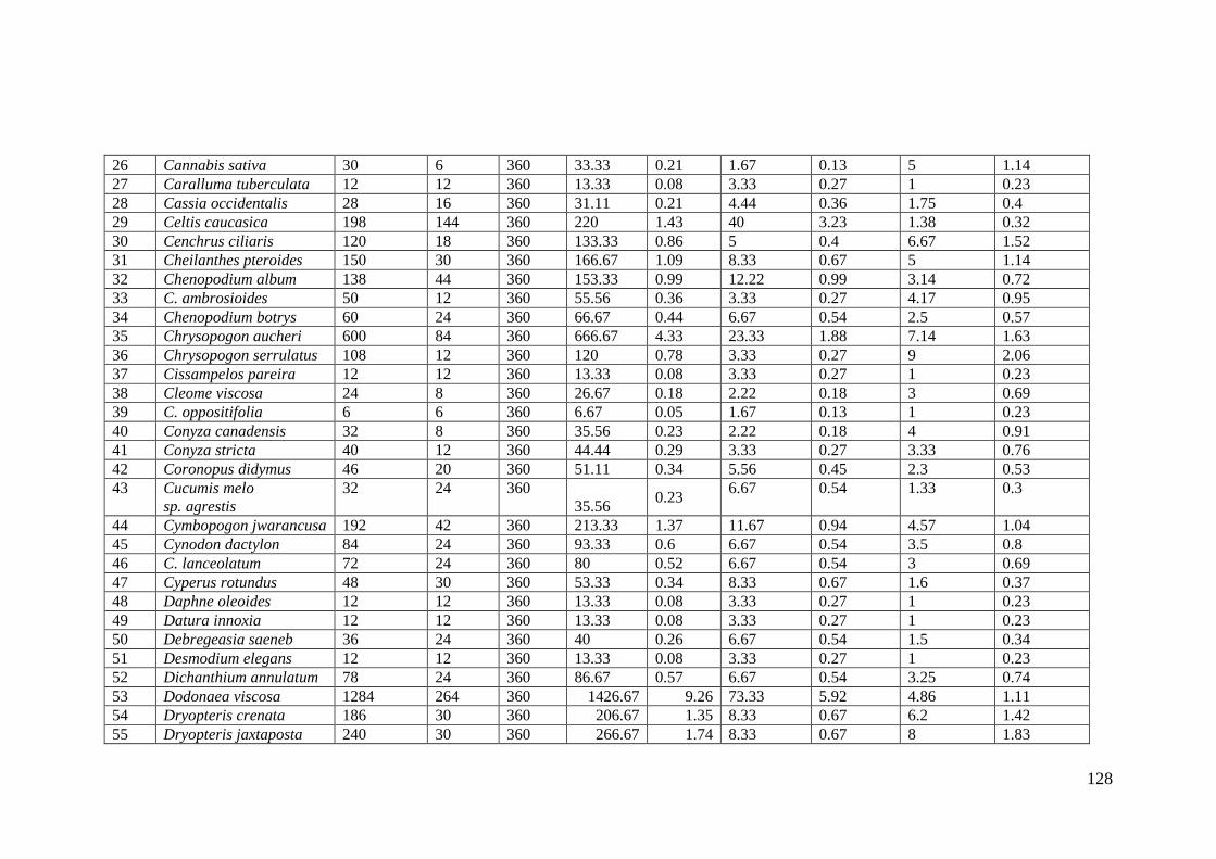
128
26 Cannabis sativa 30 6 360 33.33 0.21 1.67 0.13 5 1.14
27 Caralluma tuberculata 12 12 360 13.33 0.08 3.33 0.27 1 0.23
28 Cassia occidentalis 28 16 360 31.11 0.21 4.44 0.36 1.75 0.4
29 Celtis caucasica 198 144 360 220 1.43 40 3.23 1.38 0.32
30 Cenchrus ciliaris 120 18 360 133.33 0.86 5 0.4 6.67 1.52
31 Cheilanthes pteroides 150 30 360 166.67 1.09 8.33 0.67 5 1.14
32 Chenopodium album 138 44 360 153.33 0.99 12.22 0.99 3.14 0.72
33 C. ambrosioides 50 12 360 55.56 0.36 3.33 0.27 4.17 0.95
34 Chenopodium botrys 60 24 360 66.67 0.44 6.67 0.54 2.5 0.57
35 Chrysopogon aucheri 600 84 360 666.67 4.33 23.33 1.88 7.14 1.63
36 Chrysopogon serrulatus 108 12 360 120 0.78 3.33 0.27 9 2.06
37 Cissampelos pareira 12 12 360 13.33 0.08 3.33 0.27 1 0.23
38 Cleome viscosa 24 8 360 26.67 0.18 2.22 0.18 3 0.69
39 C. oppositifolia 6 6 360 6.67 0.05 1.67 0.13 1 0.23
40 Conyza canadensis 32 8 360 35.56 0.23 2.22 0.18 4 0.91
41 Conyza stricta 40 12 360 44.44 0.29 3.33 0.27 3.33 0.76
42 Coronopus didymus 46 20 360 51.11 0.34 5.56 0.45 2.3 0.53
43 Cucumis melo
sp. agrestis
32 24 360
35.56 0.23
6.67 0.54 1.33 0.3
44 Cymbopogon jwarancusa 192 42 360 213.33 1.37 11.67 0.94 4.57 1.04
45 Cynodon dactylon 84 24 360 93.33 0.6 6.67 0.54 3.5 0.8
46 C. lanceolatum 72 24 360 80 0.52 6.67 0.54 3 0.69
47 Cyperus rotundus 48 30 360 53.33 0.34 8.33 0.67 1.6 0.37
48 Daphne oleoides 12 12 360 13.33 0.08 3.33 0.27 1 0.23
49 Datura innoxia 12 12 360 13.33 0.08 3.33 0.27 1 0.23
50 Debregeasia saeneb 36 24 360 40 0.26 6.67 0.54 1.5 0.34
51 Desmodium elegans 12 12 360 13.33 0.08 3.33 0.27 1 0.23
52 Dichanthium annulatum 78 24 360 86.67 0.57 6.67 0.54 3.25 0.74
53 Dodonaea viscosa 1284 264 360 1426.67 9.26 73.33 5.92 4.86 1.11
54 Dryopteris crenata 186 30 360 206.67 1.35 8.33 0.67 6.2 1.42
55 Dryopteris jaxtaposta 240 30 360 266.67 1.74 8.33 0.67 8 1.83

129
56 Duchesnea indica 36 12 360 40 0.26 3.33 0.27 3 0.69
57 Ehretia obtusifolia 6 6 360 6.67 0.05 1.67 0.13 1 0.23
58 Euphorbia granulata 68 16 360 75.56 0.49 4.44 0.36 4.25 0.97
59 Euphorbia hirta 36 16 360 40 0.26 4.44 0.36 2.25 0.51
60 Euphorbia indica 48 12 360 53.33 0.34 3.33 0.27 4 0.91
61 Erioscirpus comosus 144 36 360 160 1.04 10 0.81 4 0.91
62 E. biebersteinianum 12 6 360 13.33 0.08 1.67 0.13 2 0.46
63 Ficus palmata 258 150 360 286.67 1.87 41.67 3.37 1.72 0.39
64 Ficus racemose 74 42 360 82.22 0.54 11.67 0.94 1.76 0.4
65 Fumaria indica 42 16 360 46.67 0.31 4.44 0.36 2.63 0.6
66 Geranium rotundifolium 144 24 360 160 1.04 6.67 0.54 6 1.37
67 Grewia optiva 160 102 360 177.78 1.14 28.33 2.29 1.57 0.36
68 Heliotropium strigosum 82 32 360 91.11 0.6 8.89 0.72 2.56 0.59
69 Herniaria hirsuta 56 12 360 62.22 0.41 3.33 0.27 4.67 1.07
70 Heteropogon contortus 114 24 360 126.67 0.83 6.67 0.54 4.75 1.09
71 Hyoscyamus niger 12 6 360 13.33 0.08 1.67 0.13 2 0.46
72 Imperata cylindrica 48 6 360 53.33 0.34 1.67 0.13 8 1.83
73 Indigofera heterantha 96 24 360 106.67 0.7 6.67 0.54 4 0.91
74 Isodon rugosus 12 6 360 13.33 0.08 1.67 0.13 2 0.46
75 Justicia adhatoda 210 84 360 233.33 1.5 23.33 1.88 2.5 0.57
76 Kickxia ramosissima 120 48 360 133.33 0.86 13.33 1.08 2.5 0.57
77 Lamarckia aurea 94 24 360 104.44 0.67 6.67 0.54 3.92 0.9
78 Launaea procumbens 272 60 360 302.22 1.97 16.67 1.35 4.53 1.04
79 Lotus corniculatus 12 12 360 13.33 0.08 3.33 0.27 1 0.23
80 Mallotus philippensis 234 72 360 260 1.69 20 1.62 3.25 0.74
81 Martynia annua 12 4 360 13.33 0.08 1.11 0.09 3 0.69
82 Maytenus royaleana 48 48 360 53.33 0.34 13.33 1.08 1 0.23
83 Medicago minima 12 4 360 13.33 0.08 1.11 0.09 3 0.69
84 Melia azedarach 62 42 360 68.89 0.44 11.67 0.94 1.48 0.34
85 Melothria heterophylla 6 6 360 6.67 0.05 1.67 0.13 1 0.23
86 Mentha longifolia 6 6 360 6.67 0.05 1.67 0.13 1 0.23

130
87 Micromeria biflora 72 30 360 80 0.52 8.33 0.67 2.4 0.55
88 Mimosa himalayana 24 12 360 26.67 0.18 3.33 0.27 2 0.46
89 Monotheca buxifolia 6 6 360 6.67 0.05 1.67 0.13 1 0.23
90 Morus nigra 90 72 360 100 0.65 20 1.62 1.25 0.29
91 Myrsine africana 6 6 360 6.67 0.05 1.67 0.13 1 0.23
92 Nannorrhops ritchiana 30 30 360 33.33 0.21 8.33 0.67 1 0.23
93 Nepeta griffithii 30 12 360 33.33 0.21 3.33 0.27 2.5 0.57
94 Nerium odorum 12 6 360 13.33 0.08 1.67 0.13 2 0.46
95 Olea ferruginea 576 282 360 640 4.15 78.33 6.33 2.04 0.47
96 Onosma hispida 84 36 360 93.33 0.6 10 0.81 2.33 0.53
97 Origanum vulgare 66 30 360 73.33 0.47 8.33 0.67 2.2 0.5
98 Otostegia limbata 198 60 360 220 1.43 16.67 1.35 3.3 0.75
99 Oxalis corniculata 12 4 360 13.33 0.08 1.11 0.09 3 0.69
100 Papaver pavoninum 12 8 360 13.33 0.08 2.22 0.18 1.5 0.34
101 Parthenium hysterphorus 78 24 360 86.67 0.57 6.67 0.54 3.25 0.74
102 Peganum harmala 12 4 360 13.33 0.08 1.11 0.09 3 0.69
103 Pentanema vestitum 96 16 360 106.67 0.7 4.44 0.36 6 1.37
104 Pennisetum flaccidum 48 18 360 53.33 0.34 5 0.4 2.67 0.61
105 Periploca aphylla 6 6 360 6.67 0.05 1.67 0.13 1 0.23
106 Phyllanthus niruri 24 12 360 26.67 0.18 3.33 0.27 2 0.46
107 Physalis divaricata 38 12 360 42.22 0.29 3.33 0.27 3.17 0.72
108 Pinus roxburghii 884 162 360 982.22 6.38 45 3.64 5.46 1.25
109 Piptatherum aequiglume 54 24 360 60 0.39 6.67 0.54 2.25 0.51
110 Pistacia chinensis 54 18 360 60 0.39 5 0.4 3 0.69
111 Plantago lanceolata 42 12 360 46.67 0.31 3.33 0.27 3.5 0.8
112 Plantago major 12 4 360 13.33 0.08 1.11 0.09 3 0.69
113 Poa annua 102 16 360 113.33 0.73 4.44 0.36 6.38 1.46
114 Polygala erioptera 24 6 360 26.67 0.18 1.67 0.13 4 0.91
115 Polygonum barbatum 48 12 360 53.33 0.34 3.33 0.27 4 0.91
116 Punica granatum 12 12 360 13.33 0.08 3.33 0.27 1 0.23
117 Pupalia lappacea 42 18 360 46.67 0.31 5 0.4 2.33 0.53

131
118 Quercus incana 6 6 360 6.67 0.05 1.67 0.13 1 0.23
119 Rhazya stricta 12 6 360 13.33 0.08 1.67 0.13 2 0.46
120 Rhynchosia minima 30 12 360 33.33 0.21 3.33 0.27 2.5 0.57
121 Ricinus communis 18 12 360 20 0.13 3.33 0.27 1.5 0.34
122 Rubus fruticosus 72 42 360 80 0.52 11.67 0.94 1.71 0.39
123 Rumex hastatus 42 16 360 46.67 0.31 4.44 0.36 2.63 0.6
124 Saccharum filifolium 234 36 360 260 1.69 10 0.81 6.5 1.49
125 Saccharum griffthii 126 24 360 140 0.91 6.67 0.54 5.25 1.2
126 Sageretia thea 18 18 360 20 0.13 5 0.4 1 0.23
128 Salvia lanata 30 12 360 33.33 0.21 3.33 0.27 2.5 0.57
129 Salvia moorcroftiana 96 42 360 106.67 0.7 11.67 0.94 2.29 0.52
130 Salvia plebia 24 8 360 26.67 0.18 2.22 0.18 3 0.69
131 Setaria pumila 92 16 360 102.22 0.67 4.44 0.36 5.75 1.31
132 Sida cordata 78 42 360 86.67 0.57 11.67 0.94 1.86 0.43
133 Solanum surattense 6 6 360 6.67 0.05 1.67 0.13 1 0.23
134 Stipagrostis hirtigluma 40 6 360 44.44 0.29 1.67 0.13 6.67 1.52
135 Taraxacum officinale 30 8 360 33.33 0.21 2.22 0.18 3.75 0.86
136 Tecomella undulata 6 6 360 6.67 0.05 1.67 0.13 1 0.23
137 Teucrium stocksianum 6 6 360 6.67 0.05 1.67 0.13 1 0.23
138 Tithonia sp. 48 12 360 53.33 0.34 3.33 0.27 4 0.91
139 Tribulus terestris 32 12 360 35.56 0.23 3.33 0.27 2.67 0.61
140 Trichodesma indica 48 12 360 53.33 0.34 3.33 0.27 4 0.91
141 Urtica dioica 24 12 360 26.67 0.18 3.33 0.27 2 0.46
142 Vitex negundo 16 6 360 17.78 0.1 1.67 0.13 2.67 0.61
143 Verbascum thapsus 72 36 360 80 0.52 10 0.81 2 0.46
144 Vitis jacquemontii 72 24 360 80 0.52 6.67 0.54 3 0.69
145 Withania coagulans 26 24 360 28.89 0.18 6.67 0.54 1.08 0.25
146 Woodfordia fruiticosa 60 36 360 66.67 0.44 10 0.81 1.67 0.38
147 Ziziphus mauritiana 84 42 360 93.33 0.6 11.67 0.94 2 0.46
148 Ziziphus nummularia 8 6 360 8.89 0.05 1.67 0.13 1.33 0.3
149 Zizipus oxyphyla 84 54 360 93.33 0.6 15 1.21 1.56 0.36

132
13880 4456 15422.22 100 1237.78 100 437.57 100

133
Appendix-3. Total no. of individuals, Density, Relative density, frequency, relative frequency, abundance, relative abundance considering all
undergrowth species in exotic plots.
S.no. Species name Total no. of
individuals
Quadrat
found
Total
quadrat
Density/
hac
Relative
Density
(%)
Frequency
(%)
Relative
Frequency
(%)
Abundance Relative
Abundance
(%)
1 Acacia modesta 238 72 360 264.44 1.92 20 2.07 3.31 0.94
2 Adiantum caudatum 222 42 360 246.67 1.8 11.67 1.21 5.29 1.5
3 Aerva javanica 126 36 360 140 1.02 10 1.04 3.5 0.99
4 Aerva sanguinolenta 204 30 360 226.67 1.66 8.33 0.86 6.8 1.92
5 Ailanthus altissima 78 30 360 86.67 0.64 8.33 0.86 2.6 0.74
6 Ajuga bracteosa 144 60 360 160 1.16 16.67 1.73 2.4 0.68
7 Ajuga parviflora 30 12 360 33.33 0.23 3.33 0.35 2.5 0.71
8 Alternanthera pungens 150 24 360 166.67 1.22 6.67 0.69 6.25 1.77
9 Ammi visnaga 12 4 360 13.33 0.09 1.11 0.12 3 0.85
10 Apluda mutica 120 24 360 133.33 0.96 6.67 0.69 5 1.41
11 Aristida cyanantha 174 30 360 193.33 1.4 8.33 0.86 5.8 1.64
12 Artemisia scoparia 78 24 360 86.67 0.64 6.67 0.69 3.25 0.92
13 Avena fatua 84 8 360 93.33 0.67 2.22 0.23 10.5 2.97
14 Barleria cristata 6 6 360 6.67 0.06 1.67 0.17 1 0.28
15 Bidens pilosa 96 24 360 106.67 0.79 6.67 0.69 4 1.13
16 Boerhavia procumbens 36 12 360 40 0.29 3.33 0.35 3 0.85
17 Broussonetia papyrifera 182 30 360 202.22 1.48 8.33 0.86 6.07 1.72
18 Calistemin lanceolatus 6 6 360 6.67 0.06 1.67 0.17 1 0.28
19 Commelina paludosa 110 12 360 122.22 0.9 3.33 0.35 9.17 2.6
20 Cannabis sativa 336 72 360 373.33 2.71 20 2.07 4.67 1.32
21 Caralluma tuberculata 6 6 360 6.67 0.06 1.67 0.17 1 0.28
22 Carthamus lanatus 194 44 360 215.56 1.57 12.22 1.27 4.41 1.25
23 Carthamus oxycantha 88 24 360 97.78 0.7 6.67 0.69 3.67 1.04
24 Cassia occidentalis 30 12 360 33.33 0.23 3.33 0.35 2.5 0.71
25 Celtis caucasica 52 36 360 57.78 0.41 10 1.04 1.44 0.41

134
26 Chenopodium album 216 52 360 240 1.75 14.44 1.5 4.15 1.17
27 C. ambrosioides 72 16 360 80 0.58 4.44 0.46 4.5 1.27
28 Chenopodium botrys 138 36 360 153.33 1.11 10 1.04 3.83 1.08
29 Chrysopogon aucheri 492 78 360 546.67 3.99 21.67 2.25 6.31 1.79
30 C. oppositifolia 6 6 360 6.67 0.06 1.67 0.17 1 0.28
31 Convolvulus arvense 18 4 360 20 0.15 1.11 0.12 4.5 1.27
32 Conyza Canadensis 104 16 360 115.56 0.84 4.44 0.46 6.5 1.84
33 Cucumis melo
subsp. Agrestis 12 8
360 13.33 0.09 2.22 0.23 1.5 0.42
34 Cymbopogon jwarancusa 168 42 360 186.67 1.37 11.67 1.21 4 1.13
35 Cynodon dactylon 120 18 360 133.33 0.96 5 0.52 6.67 1.89
36 C. lanceolatum 102 42 360 113.33 0.82 11.67 1.21 2.43 0.69
37 Cyperus rotundus 126 48 360 140 1.02 13.33 1.38 2.63 0.74
38 Dalbergia sissoo 12 12 360 13.33 0.09 3.33 0.35 1 0.28
39 Daphne oleoides 6 6 360 6.67 0.06 1.67 0.17 1 0.28
40 Datura innoxia 12 12 360 13.33 0.09 3.33 0.35 1 0.28
41 Debregeasia saeneb 40 30 360 44.44 0.32 8.33 0.86 1.33 0.38
42 Desmostachya bipinnata 18 12 360 20 0.15 3.33 0.35 1.5 0.42
43 Dichanthium annulatum 48 18 360 53.33 0.38 5 0.52 2.67 0.76
44 Dodonaea viscosa 1290 288 360 1433.33 10.42 80 8.3 4.48 1.27
45 Dryopteris crenata 222 30 360 246.67 1.8 8.33 0.86 7.4 2.09
46 Dryopteris jaxtaposta 96 18 360 106.67 0.79 5 0.52 5.33 1.51
47 Duchesnea indica 12 12 360 13.33 0.09 3.33 0.35 1 0.28
48 Euphorbia granulata 88 24 360 97.78 0.7 6.67 0.69 3.67 1.04
49 Euphorbia hirta 248 60 360 275.56 2.01 16.67 1.73 4.13 1.17
50 Euphorbia indica 128 32 360 142.22 1.05 8.89 0.92 4 1.13
51 Eucalyptus camaldulensis 842 180 360 935.56 6.81 50 5.19 4.68 1.32
52 Ficus palmata 156 90 360 173.33 1.25 25 2.59 1.73 0.49
53 Grewia optiva 60 30 360 66.67 0.49 8.33 0.86 2 0.57
54 Heliotropium strigosum 20 4 360 22.22 0.17 1.11 0.12 5 1.41
55 Heteropogon contortus 168 24 360 186.67 1.37 6.67 0.69 7 1.98

135
56 Isodon rugosus 6 6 360 6.67 0.06 1.67 0.17 1 0.28
57 Justicia adhatoda 126 36 360 140 1.02 10 1.04 3.5 0.99
58 Kickxia ramosissima 24 12 360 26.67 0.2 3.33 0.35 2 0.57
59 Lathyrus cicero 26 4 360 28.89 0.2 1.11 0.12 6.5 1.84
60 Launaea procumbens 108 48 360 120 0.87 13.33 1.38 2.25 0.64
61 Lotus corniculatus 66 12 360 73.33 0.52 3.33 0.35 5.5 1.56
62 Mallotus philippensis 222 78 360 246.67 1.8 21.67 2.25 2.85 0.81
63 Malva neglecta 12 4 360 13.33 0.09 1.11 0.12 3 0.85
64 Maytenus royaleana 12 12 360 13.33 0.09 3.33 0.35 1 0.28
65 Medicago minima 14 4 360 15.56 0.12 1.11 0.12 3.5 0.99
66 Melothria heterophylla 6 6 360 6.67 0.06 1.67 0.17 1 0.28
67 Mentha longifolia 6 6 360 6.67 0.06 1.67 0.17 1 0.28
68 Micromeria biflora 18 12 360 20 0.15 3.33 0.35 1.5 0.42
69 Morus alba 54 24 360 60 0.44 6.67 0.69 2.25 0.64
70 Morus nigra 88 36 360 97.78 0.7 10 1.04 2.44 0.69
71 Nannorrhops ritchiana 12 12 360 13.33 0.09 3.33 0.35 1 0.28
72 Olea ferruginea 476 192 360 528.89 3.84 53.33 5.53 2.48 0.7
73 Onosma hispida 36 18 360 40 0.29 5 0.52 2 0.57
74 Opuntia dilleni 48 24 360 53.33 0.38 6.67 0.69 2 0.57
75 Opuntia monacantha 12 12 360 13.33 0.09 3.33 0.35 1 0.28
76 Otostegia limbata 136 60 360 151.11 1.11 16.67 1.73 2.27 0.64
77 Papaver pavoninum 12 4 360 13.33 0.09 1.11 0.12 3 0.85
78 Parthenium
hysterophorus 240 36
360 266.67 1.95 10 1.04 6.67 1.89
79 Peganum harmala 6 4 360 6.67 0.06 1.11 0.12 1.5 0.42
80 Periploca aphylla 18 18 360 20 0.15 5 0.52 1 0.28
81 Phyllanthus niruri 24 12 360 26.67 0.2 3.33 0.35 2 0.57
82 Physalis divaricata 30 8 360 33.33 0.23 2.22 0.23 3.75 1.06
83 Pinus roxburghii 168 90 360 186.67 1.37 25 2.59 1.87 0.53
84 Plantago lanceolata 42 12 360 46.67 0.35 3.33 0.35 3.5 0.99
85 Plantago major 52 20 360 57.78 0.41 5.56 0.58 2.6 0.74

136
86 Polygala erioptera 72 30 360 80 0.58 8.33 0.86 2.4 0.68
87 Polygonum barbatum 114 52 360 126.67 0.93 14.44 1.5 2.19 0.62
88 Portulaca olearacea 24 8 360 26.67 0.2 2.22 0.23 3 0.85
89 Quercus incana 6 6 360 6.67 0.06 1.67 0.17 1 0.28
90 Rhazya stricta 6 6 360 6.67 0.06 1.67 0.17 1 0.28
91 Ricinus communis 30 18 360 33.33 0.23 5 0.52 1.67 0.47
92 Robinia pseudocacia 884 174 360 982.22 7.16 48.33 5.01 5.08 1.44
93 Rubus fruticosus 24 18 360 26.67 0.2 5 0.52 1.33 0.38
94 Rumex hastatus 82 42 360 91.11 0.67 11.67 1.21 1.95 0.55
95 Saccharum filifolium 276 42 360 306.67 2.24 11.67 1.21 6.57 1.86
96 Saccharum griffthii 78 54 360 86.67 0.64 15 1.56 1.44 0.41
97 Sageretia thea 18 18 360 20 0.15 5 0.52 1 0.28
98 Salix babylonica 6 6 360 6.67 0.06 1.67 0.17 1 0.28
99 Setaria pumila 76 16 360 84.44 0.61 4.44 0.46 4.75 1.34
100 Solanum nigram 16 12 360 17.78 0.12 3.33 0.35 1.33 0.38
101 Solanum surattense 60 24 360 66.67 0.49 6.67 0.69 2.5 0.71
102 Sonchus asper 60 30 360 66.67 0.49 8.33 0.86 2 0.57
103 S. graminifolium 326 36 360 362.22 2.65 10 1.04 9.06 2.56
104 Tribulus terestris 22 12 360 24.44 0.17 3.33 0.35 1.83 0.52
105 Trichodesma indica 12 4 360 13.33 0.09 1.11 0.12 3 0.85
106 Vicia sativa 36 12 360 40 0.29 3.33 0.35 3 0.85
107 Verbascum thapsus 54 12 360 60 0.44 3.33 0.35 4.5 1.27
108 Vitis jacquemontii 96 54 360 106.67 0.79 15 1.56 1.78 0.5
109 Withania coagulans 18 18 360 20 0.15 5 0.52 1 0.28
110 Xanthium sibiricum 10 4 360 11.11 0.09 1.11 0.12 2.5 0.71
111 Xanthium strumarium 18 12 360 20 0.15 3.33 0.35 1.5 0.42
12366 3470 13740 100 963.89 99.99 353.36 100

137
Appendix-4. Total no. of individuals, Density, Relative density, frequency, relative frequency, abundance, relative abundance considering only
tree undergrowth species in indigenous plots.
S.no. Species name Total no. of
individuals
Quadrat
found
Total
quadrat
Density/
hac
Relative
Density
(%)
Frequency
(%)
Relative
Frequency
(%)
Abundance Relative
Abundance
(%)
1 Acacia modesta 1128 246 360 1253.33 26.87 68.33 14.85 4.59 10.36
2 Acacia nilotica 84 66 360 93.33 1.97 18.33 3.98 1.27 2.87
3 Ailanthus altissima 64 60 360 71.11 1.55 16.67 3.62 1.07 2.42
4 Albizia lebbeck 12 12 360 13.33 0.26 3.33 0.72 1 2.26
5 Bauhinia variegata 58 24 360 64.44 1.37 6.67 1.45 2.42 5.46
6 Celtis caucasica 198 144 360 220 4.72 40 8.7 1.38 3.12
7 Debregeasia saeneb 36 24 360 40 0.86 6.67 1.45 1.5 3.39
8 Ficus palmata 258 150 360 286.67 6.18 41.67 9.06 1.72 3.88
9 Ficus racemose 74 42 360 82.22 1.8 11.67 2.54 1.76 3.97
10 Grewia optiva 160 102 360 177.78 3.78 28.33 6.16 1.57 3.54
11 Mallotus philippensis 234 72 360 260 5.58 20 4.35 3.25 7.34
12 Melia azedarach 62 42 360 68.89 1.46 11.67 2.54 1.48 3.34
13 Mimosa himalayana 24 12 360 26.67 0.6 3.33 0.72 2 4.51
14 Monotheca buxifolia 6 6 360 6.67 0.17 1.67 0.36 1 2.26
15 Morus nigra 90 72 360 100 2.15 20 4.35 1.25 2.82
16 Olea ferruginea 576 282 360 640 13.73 78.33 17.03 2.04 4.61
17 Pinus roxburghii 884 162 360 982.22 21.12 45 9.78 5.46 12.33
18 Pistacia chinensis 54 18 360 60 1.29 5 1.09 3 6.77
19 Punica granatum 12 12 360 13.33 0.26 3.33 0.72 1 2.26
20 Quercus incana 6 6 360 6.67 0.17 1.67 0.36 1 2.26
21 Tecomella undulata 6 6 360 6.67 0.17 1.67 0.36 1 2.26
22 Ziziphus mauritiana 84 42 360 93.33 1.97 11.67 2.54 2 4.51
23 Zizipus oxyphyla 84 54 360 93.33 1.97 15 3.26 1.56 3.52
4194 1656 4660 100 460 100 44.3 100
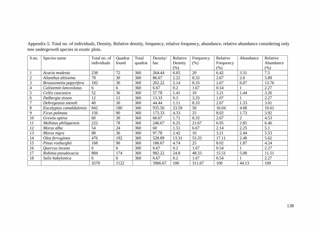
138
Appendix-5. Total no. of individuals, Density, Relative density, frequency, relative frequency, abundance, relative abundance considering only
tree undergrowth species in exotic plots.
S.no. Species name Total no. of
individuals
Quadrat
found
Total
quadrat
Density/
hac
Relative
Density
(%)
Frequency
(%)
Relative
Frequency
(%)
Abundance Relative
Abundance
(%)
1 Acacia modesta 238 72 360 264.44 6.65 20 6.42 3.31 7.5
2 Ailanthus altissima 78 30 360 86.67 2.22 8.33 2.67 2.6 5.89
3 Broussonetia papyrifera 182 30 360 202.22 5.14 8.33 2.67 6.07 13.76
4 Calistemin lanceolatus 6 6 360 6.67 0.2 1.67 0.54 1 2.27
5 Celtis caucasica 52 36 360 57.78 1.41 10 3.21 1.44 3.26
6 Dalbergia sissoo 12 12 360 13.33 0.3 3.33 1.07 1 2.27
7 Debregeasia saeneb 40 30 360 44.44 1.11 8.33 2.67 1.33 3.01
8 Eucalyptus camaldulensis 842 180 360 935.56 23.59 50 16.04 4.68 10.61
9 Ficus palmata 156 90 360 173.33 4.33 25 8.02 1.73 3.92
10 Grewia optiva 60 30 360 66.67 1.71 8.33 2.67 2 4.53
11 Mallotus philippensis 222 78 360 246.67 6.25 21.67 6.95 2.85 6.46
12 Morus alba 54 24 360 60 1.51 6.67 2.14 2.25 5.1
13 Morus nigra 88 36 360 97.78 2.42 10 3.21 2.44 5.53
14 Olea ferruginea 476 192 360 528.89 13.31 53.33 17.11 2.48 5.62
15 Pinus roxburghii 168 90 360 186.67 4.74 25 8.02 1.87 4.24
16 Quercus incana 6 6 360 6.67 0.2 1.67 0.54 1 2.27
17 Robinia pseudocacia 884 174 360 982.22 24.8 48.33 15.51 5.08 11.51
18 Salix babylonica 6 6 360 6.67 0.2 1.67 0.54 1 2.27
3570 1122 3966.67 100 311.67 100 44.13 100

139
Appendix-6.1. Shannon-Wiener diversity index (H) values considering all
undergrowth plant species recorded from Pinus roxburghii plots during spring season.
S. No Species name
Total
individuals Pi log Pi*log
Shannon-
Wiener
index
(H)
1 Acacia modesta
19 0.0 -4.1 -0.1 3.9
2 Achyranthes aspera 2 0.0 -6.3 0.0
3 Adiantum caudatum 19 0.0 -4.1 -0.1
4 Aerva sanguinolenta 19 0.0 -4.1 -0.1
5 Ajuga bracteosa 8 0.0 -4.9 0.0
6 Ajuga parviflora 4 0.0 -5.6 0.0
7 Ammi visnaga 3 0.0 -5.9 0.0
8 Anisomeles indica 5 0.0 -5.4 0.0
9 Aristida cyanantha 26 0.0 -3.8 -0.1
10 Asparagus adscendens 5 0.0 -5.4 0.0
11 Bauhinia variegata 9 0.0 -4.8 0.0
12 Barleria cristata 7 0.0 -5.1 0.0
13 Bidens pilosa 2 0.0 -6.3 0.0
14 Boerhavia procumbens 10 0.0 -4.7 0.0
15 Brachiaria ramosa 23 0.0 -3.9 -0.1
17 Cassia occidentalis 4 0.0 -5.6 0.0
18 Celtis caucasica 15 0.0 -4.3 -0.1
19 Chenopodium ambrosioides 11 0.0 -4.6 0.0
20 Cheilanthes pteroides 25 0.0 -3.8 -0.1
21 Chrysopogon aucheri 41 0.0 -3.3 -0.1
22 Cissampelos pareira 2 0.0 -6.3 0.0
23 Conyza stricta 7 0.0 -5.1 0.0
24 Conyza canadensis 6 0.0 -5.2 0.0
25 Cynodon dactylon 14 0.0 -4.4 -0.1
26 Cynoglossum lanceolatum 12 0.0 -4.5 0.0
27 Daphne oleoides 2 0.0 -6.3 0.0
28 Debregeasia saeneb 6 0.0 -5.2 0.0
29 Desmodium elegans 2 0.0 -6.3 0.0
30 Dichanthium annulatum 13 0.0 -4.5 -0.1
31 Dodonaea viscosa 85 0.1 -2.6 -0.2
32 Dryopteris crenata 31 0.0 -3.6 -0.1
33 Dryopteris jaxtaposta 40 0.0 -3.3 -0.1
34 Erioscirpus comosus 24 0.0 -3.8 -0.1
35 Euphorbia granulata 13 0.0 -4.5 -0.1
36 Euphorbia hirta 2 0.0 -6.3 0.0
37 Euphorbia indica 8 0.0 -4.9 0.0

140
38 Ficus palmata 19 0.0 -4.1 -0.1
39 Ficus racemosa 12 0.0 -4.5 0.0
40 Fumaria indica 7 0.0 -5.1 0.0
41 Geranium rotundifolium 24 0.0 -3.8 -0.1
42 Heteropogon contortus 19 0.0 -4.1 -0.1
43 Imperata cylindrica 8 0.0 -4.9 0.0
44 Indigofera heterantha 16 0.0 -4.2 -0.1
45 Kickxia ramosissima 7 0.0 -5.1 0.0
46 Launaea procumbens 14 0.0 -4.4 -0.1
47 Mallotus philippensis 35 0.0 -3.5 -0.1
48 Medicago minima 2 0.0 -6.3 0.0
49 Micromeria biflora 10 0.0 -4.7 0.0
50 Mimosa himalayana 4 0.0 -5.6 0.0
51 Morus nigra 7 0.0 -5.1 0.0
52 Nannorrhops ritchiana 3 0.0 -5.9 0.0
53 Nepeta griffithii 5 0.0 -5.4 0.0
54 Olea ferruginea 36 0.0 -3.4 -0.1
55 Origanum vulgare 11 0.0 -4.6 0.0
56 Otostegia limbata 11 0.0 -4.6 0.0
57 Oxalis corniculata L. 2 0.0 -6.3 0.0
58 Periploca aphylla 1 0.0 -7.0 0.0
59 Phyllanthus niruri 4 0.0 -5.6 0.0
60 Physalis divaricata 2 0.0 -6.3 0.0
61 Pinus roxburghii 143 0.1 -2.1 -0.3
62 Piptatherum aequiglume 9 0.0 -4.8 0.0
63 Pistacia chinensis 9 0.0 -4.8 0.0
64 Plantago lanceolata 7 0.0 -5.1 0.0
65 Polygala erioptera 4 0.0 -5.6 0.0
66 poa annua 19 0.0 -4.1 -0.1
67 Punica granatum 2 0.0 -6.3 0.0
68 Quercus incana 1 0.0 -7.0 0.0
69 Rhynchosia minima 5 0.0 -5.4 0.0
70 Rubus fruticosus 12 0.0 -4.5 0.0
71 Rumex hastatus 7 0.0 -5.1 0.0
72 launaea procumbens 28 0.0 -3.7 -0.1
73 Sageretia thea 3 0.0 -5.9 0.0
74 Setaria pumila 17 0.0 -4.2 -0.1
75 Sida cordata 7 0.0 -5.1 0.0
76 Stipagrostis hirtigluma 5 0.0 -5.4 0.0
77 Taraxacum officinale 5 0.0 -5.4 0.0
78 Tribulus terestris 4 0.0 -5.6 0.0
79 Urtica dioica 4 0.0 -5.6 0.0

141
80 Verbascum Thapsus 10 0.0 -4.7 0.0
81 Vitis jacquemontii 12 0.0 -4.5 0.0
82 Woodfordia fruiticosa 10 0.0 -4.7 0.0
83 Zizypus oxyphyla 14 0.0 -4.4 -0.1
Total 1120 -3.9

142
Appendix-6.2. Shannon-Wiener diversity index (H) values considering all undergrowth
plant species recorded from Pinus roxburghii plots during monsoon season.
S. No Species name
Total
individuals Pi log Pi*log
Shannon-
Wiener
index (H)
1 Acacia modesta 23 0.02 -4.03 -0.07 3.95
2 Achyranthes aspera 2 0.00 -6.48 -0.01
3 Adiantum caudatum 22 0.02 -4.08 -0.07
4 Aerva sanguinolenta 24 0.02 -3.99 -0.07
5 Ajuga bracteosa 13 0.01 -4.60 -0.05
6 Ajuga parviflora 12 0.01 -4.68 -0.04
7 Ammi visnaga 6 0.00 -5.38 -0.02
8 Anisomeles indica 8 0.01 -5.09 -0.03
9 Aristida cyanantha 26 0.02 -3.91 -0.08
10 Asparagus adscendens 6 0.00 -5.38 -0.02
11 Bauhinia variegata 11 0.01 -4.77 -0.04
12 Barleria cristata 7 0.01 -5.22 -0.03
13 Bidens pilosa 2 0.00 -6.48 -0.01
14 Boerhavia procumbens 10 0.01 -4.87 -0.04
15 Brachiaria ramosa 23 0.02 -4.03 -0.07
17 Cassia occidentalis 4 0.00 -5.78 -0.02
18 Celtis caucasica 18 0.01 -4.28 -0.06
19 Chenopodium ambrosioides 14 0.01 -4.53 -0.05
20 Cheilanthes pteroides 25 0.02 -3.95 -0.08
21 Chrysopogon aucheri 41 0.03 -3.46 -0.11
22 Cissampelos pareira 2 0.00 -6.48 -0.01
23 Conyza stricta 13 0.01 -4.60 -0.05
24 Conyza canadensis 10 0.01 -4.87 -0.04
25 Cynodon dactylon 14 0.01 -4.53 -0.05
26 Cynoglossum lanceolatum 12 0.01 -4.68 -0.04
27 Daphne oleoides 2 0.00 -6.48 -0.01
28 Debregeasia saeneb 6 0.00 -5.38 -0.02
29 Desmodium elegans 2 0.00 -6.48 -0.01
30 Dichanthium annulatum 13 0.01 -4.60 -0.05
31 Dodonaea viscosa 85 0.07 -2.73 -0.18
32 Dryopteris crenata 31 0.02 -3.74 -0.09
33 Dryopteris jaxtaposta 40 0.03 -3.48 -0.11
34 Erioscirpus comosus 24 0.02 -3.99 -0.07
35 Euphorbia granulata 21 0.02 -4.12 -0.07
36 Euphorbia hirta 4 0.00 -5.78 -0.02
37 Euphorbia indica 16 0.01 -4.40 -0.05

143
38 Ficus palmata 21 0.02 -4.12 -0.07
39 Ficus racemosa 13 0.01 -4.60 -0.05
40 Fumaria indica 14 0.01 -4.53 -0.05
41 Geranium rotundifolium 24 0.02 -3.99 -0.07
42 Heteropogon contortus 19 0.01 -4.22 -0.06
43 Imperata cylindrica 8 0.01 -5.09 -0.03
44 Indigofera heterantha 16 0.01 -4.40 -0.05
45 Kickxia ramosissima 7 0.01 -5.22 -0.03
46 Launaea procumbens 24 0.02 -3.99 -0.07
47 Mallotus philippensis 38 0.03 -3.53 -0.10
48 Medicago minima 4 0.00 -5.78 -0.02
49 Micromeria biflora 10 0.01 -4.87 -0.04
50 Mimosa himalayana 4 0.00 -5.78 -0.02
51 Morus nigra 8 0.01 -5.09 -0.03
52 Nannorrhops ritchiana 3 0.00 -6.07 -0.01
53 Nepeta griffithii 10 0.01 -4.87 -0.04
54 Olea ferruginea 40 0.03 -3.48 -0.11
55 Origanum vulgare 11 0.01 -4.77 -0.04
56 Otostegia limbata 11 0.01 -4.77 -0.04
57 Oxalis corniculata 4 0.00 -5.78 -0.02
58 Periploca aphylla 1 0.00 -7.17 -0.01
59 Phyllanthus niruri 4 0.00 -5.78 -0.02
60 Physalis divaricata 4 0.00 -5.78 -0.02
61 Pinus roxburghii 156 0.12 -2.12 -0.25
62 Piptatherum aequiglume 9 0.01 -4.97 -0.03
63 Pistacia chinensis 9 0.01 -4.97 -0.03
64 Plantago lanceolata 14 0.01 -4.53 -0.05
65 Polygala erioptera 4 0.00 -5.78 -0.02
66 poa annua 32 0.02 -3.70 -0.09
67 Punica granatum 2 0.00 -6.48 -0.01
68 Quercus incana 1 0.00 -7.17 -0.01
69 Rhynchosia minima 5 0.00 -5.56 -0.02
70 Rubus fruticosus 12 0.01 -4.68 -0.04
71 Rumex hastatus 14 0.01 -4.53 -0.05
72 launaea procumbens 28 0.02 -3.84 -0.08
73 Sageretia thea 3 0.00 -6.07 -0.01
74 Setaria pumila 29 0.02 -3.80 -0.08
75 Sida cordata 7 0.01 -5.22 -0.03
76 Stipagrostis hirtigluma 10 0.01 -4.87 -0.04
77 Taraxacum officinale 10 0.01 -4.87 -0.04
78 Tribulus terestris 8 0.01 -5.09 -0.03
79 Urtica dioica 4 0.00 -5.78 -0.02

144
80 Verbascum Thapsus 16 0.01 -4.40 -0.05
81 Vitis jacquemontii 12 0.01 -4.68 -0.04
82 Woodfordia fruiticosa 10 0.01 -4.87 -0.04
83 Zizypus oxyphyla 14 0.01 -4.53 -0.05
1299 -3.95

145
Appendix-6.3 Shannon-Wiener diversity index (H) values considering all undergrowth
plant species recorded from Pinus roxburghii plots during winter season.
S. No Species name
Total
individuals Pi log Pi*log
Shannon-
Wiener
index
(H)
1 Acacia modesta 19 0.0 -3.9 -0.1 3.6
2 Achyranthes aspera 2 0.0 -6.2 0.0
3 Adiantum caudatum 19 0.0 -3.9 -0.1
4 Aerva sanguinolenta 19 0.0 -3.9 -0.1
5 Ajuga bracteosa 8 0.0 -4.8 0.0
6 Ajuga parviflora 4 0.0 -5.5 0.0
7 Ammi visnaga 0 0.0 0.0 0.0
8 Anisomeles indica 5 0.0 -5.3 0.0
9 Aristida cyanantha 26 0.0 -3.6 -0.1
10 Asparagus adscendens 5 0.0 -5.3 0.0
11 Bauhinia variegata 9 0.0 -4.7 0.0
12 Barleria cristata 7 0.0 -4.9 0.0
13 Bidens pilosa 0 0.0 0.0 0.0
14 Boerhavia procumbens 10 0.0 -4.6 0.0
15 Brachiaria ramosa 0 0.0 0.0 0.0
17 Cassia occidentalis 0 0.0 0.0 0.0
18 Celtis caucasica 15 0.0 -4.2 -0.1
19 Chenopodium ambrosioides 0 0.0 0.0 0.0
20 Cheilanthes pteroides 25 0.0 -3.7 -0.1
21 Chrysopogon aucheri 41 0.0 -3.2 -0.1
22 Cissampelos pareira 2 0.0 -6.2 0.0
23 Conyza stricta 0 0.0 0.0 0.0
24 Conyza canadensis 0 0.0 0.0 0.0
25 Cynodon dactylon 14 0.0 -4.2 -0.1
26 Cynoglossum lanceolatum 12 0.0 -4.4 -0.1
27 Daphne oleoides 2 0.0 -6.2 0.0
28 Debregeasia saeneb 6 0.0 -5.1 0.0
29 Desmodium elegans 2 0.0 -6.2 0.0
30 Dichanthium annulatum 13 0.0 -4.3 -0.1
31 Dodonaea viscosa 85 0.1 -2.4 -0.2
32 Dryopteris crenata 31 0.0 -3.4 -0.1
33 Dryopteris jaxtaposta 40 0.0 -3.2 -0.1
34 Erioscirpus comosus 24 0.0 -3.7 -0.1
35 Euphorbia granulata 0 0.0 0.0 0.0
36 Euphorbia hirta 0 0.0 0.0 0.0

146
37 Euphorbia indica 0 0.0 0.0 0.0
38 Ficus palmata 19 0.0 -3.9 -0.1
39 Ficus racemosa 12 0.0 -4.4 -0.1
40 Fumaria indica 0 0.0 0.0 0.0
41 Geranium rotundifolium 24 0.0 -3.7 -0.1
42 Heteropogon contortus 19 0.0 -3.9 -0.1
43 Imperata cylindrica 8 0.0 -4.8 0.0
44 Indigofera heterantha 16 0.0 -4.1 -0.1
45 Kickxia ramosissima 7 0.0 -4.9 0.0
46 Launaea procumbens 14 0.0 -4.2 -0.1
47 Mallotus philippensis 35 0.0 -3.3 -0.1
48 Medicago minima 0 0.0 0.0 0.0
49 Micromeria biflora 10 0.0 -4.6 0.0
50 Mimosa himalayana 4 0.0 -5.5 0.0
51 Morus nigra 7 0.0 -4.9 0.0
52 Nannorrhops ritchiana 3 0.0 -5.8 0.0
53 Nepeta griffithii 0 0.0 0.0 0.0
54 Olea ferruginea 36 0.0 -3.3 -0.1
55 Origanum vulgare 11 0.0 -4.5 -0.1
56 Otostegia limbata 11 0.0 -4.5 -0.1
57 Oxalis corniculata 0 0.0 0.0 0.0
58 Periploca aphylla 1 0.0 -6.9 0.0
59 Phyllanthus niruri 4 0.0 -5.5 0.0
60 Physalis divaricata 0 0.0 0.0 0.0
61 Pinus roxburghii 143 0.1 -1.9 -0.3
62 Piptatherum aequiglume 9 0.0 -4.7 0.0
63 Pistacia chinensis 9 0.0 -4.7 0.0
64 Plantago lanceolata 0 0.0 0.0 0.0
65 Polygala erioptera 4 0.0 -5.5 0.0
66 poa annua 0 0.0 0.0 0.0
67 Punica granatum 2 0.0 -6.2 0.0
68 Quercus incana 1 0.0 -6.9 0.0
69 Rhynchosia minima 5 0.0 -5.3 0.0
70 Rubus fruticosus 12 0.0 -4.4 -0.1
71 Rumex hastatus 0 0.0 0.0 0.0
72 launaea procumbens 28 0.0 -3.5 -0.1
73 Sageretia thea 3 0.0 -5.8 0.0
74 Setaria pumila 0 0.0 0.0 0.0
75 Sida cordata 7 0.0 -4.9 0.0
76 Stipagrostis hirtigluma 5 0.0 -5.3 0.0
77 Taraxacum officinale 0 0.0 0.0 0.0
78 Tribulus terestris 4 0.0 -5.5 0.0

147
79 Urtica dioica 4 0.0 -5.5 0.0
80 Verbascum Thapsus 10 0.0 -4.6 0.0
81 Vitis jacquemontii 12 0.0 -4.4 -0.1
82 Woodfordia fruiticosa 10 0.0 -4.6 0.0
83 Zizypus oxyphyla 14 0.0 -4.2 -0.1
968 -3.6

148
Appendix-6.4 Shannon-Wiener diversity index (H) values considering undergrowth
tree species only recorded from Pinus roxburghii plots during summer season.
S. No Species name
Total
individuals Pi log Pi*log
Shannon-
Wiener
index
(H)
1 Acacia modesta 19 0.06 -2.86 -0.16 2.01
2 Bauhinia variegata 9 0.03 -3.60 -0.10
3 Celtis caucasica 15 0.05 -3.09 -0.14
4 Debregeasia saeneb 6 0.02 -4.01 -0.07
5 Ficus palmata 19 0.06 -2.86 -0.16
6 Ficus racemosa 12 0.04 -3.32 -0.12
7 Mallotus philippensis 35 0.11 -2.25 -0.24
8 Mimosa himalayana 4 0.01 -4.42 -0.05
9 Morus nigra 7 0.02 -3.86 -0.08
10 Olea ferruginea 36 0.11 -2.22 -0.24
11 Pinus roxburghii 143 0.43 -0.84 -0.36
12 Pistacia chinensis 9 0.03 -3.60 -0.10
13 Punica granatum 2 0.01 -5.11 -0.03
14 Quercus incana 1 0.00 -5.80 -0.02
15 Zizypus oxyphyla 14 0.04 -3.16 -0.13
331 -2.01

149
Appendix-6.5. Shannon-Wiener diversity index (H) values considering undergrowth
tree species only recorded from Pinus roxburghii plots during monsoon season.
S. No Species name
Total
individuals Pi Log Pi*log
Shannon-
Wiener
index
(H)
1 Acacia modesta 23 0.06 -2.76 -0.17 2.01
2 Bauhinia variegata 11 0.03 -3.50 -0.11
3 Celtis caucasica 18 0.05 -3.01 -0.15
4 Debregeasia saeneb 6 0.02 -4.11 -0.07
5 Ficus palmata 21 0.06 -2.85 -0.16
6 Ficus racemosa 13 0.04 -3.33 -0.12
7 Mallotus philippensis 38 0.10 -2.26 -0.24
8 Mimosa himalayana 4 0.01 -4.51 -0.05
9 Morus nigra 8 0.02 -3.82 -0.08
10 Olea ferruginea 40 0.11 -2.21 -0.24
11 Pinus roxburghii 156 0.43 -0.85 -0.36
12 Pistacia chinensis 9 0.02 -3.70 -0.09
13 Punica granatum 2 0.01 -5.20 -0.03
14 Quercus incana 1 0.00 -5.90 -0.02
15 Zizypus oxyphyla 14 0.04 -3.26 -0.13
364 -2.01

150
Appendix-6.6. Shannon-Wiener diversity index (H) values considering undergrowth
tree species only recorded from Pinus roxburghii plots during winter season.
S. No Species name
Total
individuals Pi log Pi*log
Shannon-
Wiener
index
(H)
1 Acacia modesta 19 0.06 -2.86 -0.16 2.01
2 Bauhinia variegata 9 0.03 -3.60 -0.10
3 Celtis caucasica 15 0.05 -3.09 -0.14
4 Debregeasia saeneb 6 0.02 -4.01 -0.07
5 Ficus palmata 19 0.06 -2.86 -0.16
6 Ficus racemosa 12 0.04 -3.32 -0.12
7 Mallotus philippensis 35 0.11 -2.25 -0.24
8 Mimosa himalayana 4 0.01 -4.42 -0.05
9 Morus nigra 7 0.02 -3.86 -0.08
10 Olea ferruginea 36 0.11 -2.22 -0.24
11 Pinus roxburghii 143 0.43 -0.84 -0.36
12 Pistacia chinensis 9 0.03 -3.60 -0.10
13 Punica granatum 2 0.01 -5.11 -0.03
14 Quercus incana 1 0.00 -5.80 -0.02
15 Zizypus oxyphyla 14 0.04 -3.16 -0.13
331 -2.01

151
Appendix-6.7. Shannon-Wiener diversity index (H) values considering all
undergrowth plant species recorded from E. camaldulensis plots during spring season.
S.no Species name Total
indivi.
Pi log
Pi*log
Shannon-
Wiener
index
(H)
1 Aerva javanica 21 0.0 -3.9 -0.1 1
2 Acacia modesta 39 0.0 -3.2 -0.1 2
3 Adiantum caudatum 37 0.0 -3.3 -0.1 3
4 Ajuga bracteosa 11 0.0 -4.5 0.0 4
5 Ajuga parviflora 5 0.0 -5.3 0.0 5
6 Aristida cyanantha 29 0.0 -3.5 -0.1 6
7 Barleria cristata 1 0.0 -6.9 0.0 7
8 Bidens pilosa 15 0.0 -4.2 -0.1 8
9 Boerhavia procumbens 6 0.0 -5.1 0.0 9
10 Cannabis sativa 16 0.0 -4.1 -0.1 10
11 Caralluma tuberculata 1 0.0 -6.9 0.0 11
12 Celtis caucasica 8 0.0 -4.8 0.0 12
13 Chenopodium album 20 0.0 -3.9 -0.1 13
14 Chenopodium botrys 23 0.0 -3.8 -0.1 14
15 Chrysopogon aucheri 31 0.0 -3.5 -0.1 15
16 Colebrookea oppositifolia 1 0.0 -6.9 0.0 16
17 Cymbopogon jwarancusa 28 0.0 -3.6 -0.1 17
18 Cynoglossum lanceolatum 11 0.0 -4.5 0.0 18
19 Cyperus rotundus 21 0.0 -3.9 -0.1 19
20 Daphne oleoides 1 0.0 -6.9 0.0 20
21 Datura innoxia 2 0.0 -6.2 0.0 21
22 Debregeasia saeneb 6 0.0 -5.1 0.0 22
23 Desmostachya bipinnata 3 0.0 -5.8 0.0 23
24 Dichanthium annulatum 8 0.0 -4.8 0.0 24
25 Dodonea viscosa 123 0.1 -2.1 -0.3 25
26 Dryopteris crenata 37 0.0 -3.3 -0.1 26
27 Dryopteris jaxtaposta 16 0.0 -4.1 -0.1 27
28 Duchesnea indica 2 0.0 -6.2 0.0 28
29 Eucalyptus camaldulensis 139 0.1 -2.0 -0.3 29
30 Euphorbia granulate 2 0.0 -6.2 0.0 30
31 Euphorbia hirta 14 0.0 -4.3 -0.1 31
32 Euphorbia indica 12 0.0 -4.4 -0.1 32
33 Ficus palmata 8 0.0 -4.8 0.0 33
34 Grevia optiva 10 0.0 -4.6 0.0 34
35 Heteropogan contortus 14 0.0 -4.3 -0.1 35
36 Justicia adhatoda 21 0.0 -3.9 -0.1 36
37 Kickxia ramosissima 2 0.0 -6.2 0.0 37
38 Launaea procumbens 5 0.0 -5.3 0.0 38
39 Mallotus philippensis 36 0.0 -3.3 -0.1 39
40 Maytenus royaleanus 2 0.0 -6.2 0.0 40
41 Mentha longifolia 1 0.0 -6.9 0.0 41

152
42 Micromeria biflora 3 0.0 -5.8 0.0 42
43 Nannorrhops ritchiana 2 0.0 -6.2 0.0 43
44 Olea ferruginea 35 0.0 -3.4 -0.1 44
45 Onosma hispida 6 0.0 -5.1 0.0 45
46 Opuntia dilleni 8 0.0 -4.8 0.0 46
47 Opuntia monacantha 2 0.0 -6.2 0.0 47
48 Otostegia limbata 18 0.0 -4.0 -0.1 48
49 Parthenium hysterophorus 12 0.0 -4.4 -0.1 49
50 Peganum harmala 1 0.0 -6.9 0.0 50
51 Periploca aphylla 3 0.0 -5.8 0.0 51
52 Phyllanthus niruri 2 0.0 -6.2 0.0 52
53 Pinus roxburghii 27 0.0 -3.6 -0.1 53
54 Plantago lanceolata 1 0.0 -6.9 0.0 54
55 Plantago major 1 0.0 -6.9 0.0 55
56 Isodon rugosus 1 0.0 -6.9 0.0 56
57 Polygonum barbatum 10 0.0 -4.6 0.0 57
58 Quercus incana 1 0.0 -6.9 0.0 58
59 Rhazya stricta 1 0.0 -6.9 0.0 59
60 Ricinus communis 2 0.0 -6.2 0.0 60
61 Rubus fruticosus 4 0.0 -5.5 0.0 61
62 Rumex hastatus 4 0.0 -5.5 0.0 62
63 Saccharum griffthii 13 0.0 -4.3 -0.1 63
64 Saccharum filifolium 16 0.0 -4.1 -0.1 64
65 Sageretia thea 3 0.0 -5.8 0.0 65
66 Solanum surattense 2 0.0 -6.2 0.0 66
67 Symphyotrichum graminifolium 18 0.0 -4.0 -0.1 67
68 Verbascum Thapsus 9 0.0 -4.7 0.0 68
69 Vitis jacquemontii 8 0.0 -4.8 0.0 69
70 Withania coagulans 3 0.0 -5.8 0.0 70
1004 -3.5

153
Appendix- 6.8. Shannon-Wiener diversity index (H) values considering all
undergrowth plant species recorded from E. camaldulensis plots during monsoon
season.
S. No Species name
Total
individuals Pi log Pi*log
Shannon-
Wiener
index
(H)
1 Aerva javanica 21 0.0 -4.0 -0.1 3.4
2 Acacia modesta 41 0.0 -3.3 -0.1
3 Adiantum caudatum 37 0.0 -3.4 -0.1
4 Ajuga bracteosa 11 0.0 -4.6 0.0
5 Ajuga parviflora 5 0.0 -5.4 0.0
6 Aristida cyanantha 29 0.0 -3.7 -0.1
7 Barleria cristata 1 0.0 -7.0 0.0
8 Bidens pilosa 19 0.0 -4.1 -0.1
9 Boerhavia procumbens 6 0.0 -5.2 0.0
10 Cannabis sativa 16 0.0 -4.3 -0.1
11 Caralluma tuberculata 1 0.0 -7.0 0.0
12 Celtis caucasica 10 0.0 -4.7 0.0
13 Chenopodium album 34 0.0 -3.5 -0.1
14 Chenopodium botrys 23 0.0 -3.9 -0.1
15 Chrysopogon aucheri 31 0.0 -3.6 -0.1
16 Colebrookea oppositifolia 1 0.0 -7.0 0.0
17 Cymbopogon jwarancusa 28 0.0 -3.7 -0.1
18 Cynoglossum lanceolatum 11 0.0 -4.6 0.0
19 Cyperus rotundus 21 0.0 -4.0 -0.1
20 Daphne oleoides 1 0.0 -7.0 0.0
21 Datura innoxia 2 0.0 -6.3 0.0
22 Debregeasia saeneb 8 0.0 -4.9 0.0
23 Desmostachya bipinnata 3 0.0 -5.9 0.0
24 Dichanthium annulatum 8 0.0 -4.9 0.0
25 Dodonea viscosa 123 0.1 -2.2 -0.2
26 Dryopteris crenata 37 0.0 -3.4 -0.1
27 Dryopteris jaxtaposta 16 0.0 -4.3 -0.1
28 Duchesnea indica 2 0.0 -6.3 0.0
29 Eucalyptus camaldulensis 143 0.1 -2.1 -0.3
30 Euphorbia granulate 4 0.0 -5.6 0.0
31 Euphorbia hirta 23 0.0 -3.9 -0.1
32 Euphorbia indica 24 0.0 -3.8 -0.1
33 Ficus palmata 10 0.0 -4.7 0.0
34 Grevia optiva 10 0.0 -4.7 0.0
35 Heteropogan contortus 14 0.0 -4.4 -0.1

154
36 Justicia adhatoda 21 0.0 -4.0 -0.1
37 Kickxia ramosissima 2 0.0 -6.3 0.0
38 Launaea procumbens 5 0.0 -5.4 0.0
39 Mallotus philippensis 39 0.0 -3.4 -0.1
40 Maytenus royaleanus 2 0.0 -6.3 0.0
41 Mentha longifolia 1 0.0 -7.0 0.0
42 Micromeria biflora 3 0.0 -5.9 0.0
43 Nannorrhops ritchiana 2 0.0 -6.3 0.0
44 Olea ferruginea 37 0.0 -3.4 -0.1
45 Onosma hispida 6 0.0 -5.2 0.0
46 Opuntia dilleni 8 0.0 -4.9 0.0
47 Opuntia monacantha 2 0.0 -6.3 0.0
48 Otostegia limbata 32 0.0 -3.6 -0.1
49 Parthenium hysterophorus 12 0.0 -4.5 0.0
50 Peganum harmala 2 0.0 -6.3 0.0
51 Periploca aphylla 3 0.0 -5.9 0.0
52 Phyllanthus niruri 2 0.0 -6.3 0.0
53 Pinus roxburghii 30 0.0 -3.6 -0.1
54 Plantago lanceolata 2 0.0 -6.3 0.0
55 Plantago major 2 0.0 -6.3 0.0
56 Isodon rugosus 1 0.0 -7.0 0.0
57 Polygonum barbatum 21 0.0 -4.0 -0.1
58 Quercus incana 1 0.0 -7.0 0.0
59 Rhazya stricta 1 0.0 -7.0 0.0
60 Ricinus communis 2 0.0 -6.3 0.0
61 Rubus fruticosus 4 0.0 -5.6 0.0
62 Rumex hastatus 8 0.0 -4.9 0.0
63 Saccharum griffthii 13 0.0 -4.5 -0.1
64 Saccharum filifolium 16 0.0 -4.3 -0.1
65 Sageretia thea 3 0.0 -5.9 0.0
66 Solanum surattense 2 0.0 -6.3 0.0
67 Symphyotrichum graminifolium 34 0.0 -3.5 -0.1
68 Verbascum Thapsus 18 0.0 -4.1 -0.1
69 Vitis jacquemontii 8 0.0 -4.9 0.0
70 Withania coagulans 3 0.0 -5.9 0.0
1122 -3.4

155
Appendix-6.9. Shannon-Wiener diversity index (H) values considering all undergrowth
plant species recorded from E. camaldulensis plots during winter season.
S. No Species name
Total
individuals Pi log Pi*log
Shannon-
Wiener
index (H)
1 Aerva javanica 21 0.0 -3.8 -0.1 3.3
2 Acacia modesta 39 0.0 -3.1 -0.1
3 Adiantum caudatum 37 0.0 -3.2 -0.1
4 Ajuga bracteosa 11 0.0 -4.4 -0.1
5 Ajuga parviflora 5 0.0 -5.2 0.0
6 Aristida cyanantha 29 0.0 -3.4 -0.1
7 Barleria cristata 1 0.0 -6.8 0.0
8 Bidens pilosa 0 0.0 0.0 0.0
9 Boerhavia procumbens 6 0.0 -5.0 0.0
10 Cannabis sativa 16 0.0 -4.0 -0.1
11 Caralluma tuberculata 1 0.0 -6.8 0.0
12 Celtis caucasica 8 0.0 -4.7 0.0
13 Chenopodium album 0 0.0 0.0 0.0
14 Chenopodium botrys 23 0.0 -3.7 -0.1
15 Chrysopogon aucheri 31 0.0 -3.4 -0.1
16 Colebrookea oppositifolia 1 0.0 -6.8 0.0
17 Cymbopogon jwarancusa 28 0.0 -3.5 -0.1
18 Cynoglossum lanceolatum 11 0.0 -4.4 -0.1
19 Cyperus rotundus 21 0.0 -3.8 -0.1
20 Daphne oleoides 1 0.0 -6.8 0.0
21 Datura innoxia 2 0.0 -6.1 0.0
22 Debregeasia saeneb 6 0.0 -5.0 0.0
23 Desmostachya bipinnata 3 0.0 -5.7 0.0
24 Dichanthium annulatum 8 0.0 -4.7 0.0
25 Dodonea viscosa 123 0.1 -2.0 -0.3
26 Dryopteris crenata 37 0.0 -3.2 -0.1
27 Dryopteris jaxtaposta 16 0.0 -4.0 -0.1
28 Duchesnea indica 2 0.0 -6.1 0.0
29 Eucalyptus camaldulensis 139 0.2 -1.9 -0.3
30 Euphorbia granulata 0 0.0 0.0 0.0
31 Euphorbia hirta 0 0.0 0.0 0.0
32 Euphorbia indica 0 0.0 0.0 0.0
33 Ficus palmata 8 0.0 -4.7 0.0
34 Grevia optiva 10 0.0 -4.5 -0.1
35 Heteropogan contortus 14 0.0 -4.2 -0.1
36 Justicia adhatoda 21 0.0 -3.8 -0.1

156
37 Kickxia ramosissima 2 0.0 -6.1 0.0
38 Launaea procumbens 5 0.0 -5.2 0.0
39 Mallotus philippensis 36 0.0 -3.2 -0.1
40 Maytenus royaleanus 2 0.0 -6.1 0.0
41 Mentha longifolia 1 0.0 -6.8 0.0
42 Micromeria biflora 3 0.0 -5.7 0.0
43 Nannorrhops ritchiana 2 0.0 -6.1 0.0
44 Olea ferruginea 35 0.0 -3.2 -0.1
45 Onosma hispida 6 0.0 -5.0 0.0
46 Opuntia dilleni 8 0.0 -4.7 0.0
47 Opuntia monacantha 2 0.0 -6.1 0.0
48 Otostegia limbata 18 0.0 -3.9 -0.1
49 Parthenium hysterophorus 12 0.0 -4.3 -0.1
50 Peganum harmala 0 0.0 0.0 0.0
51 Periploca aphylla 3 0.0 -5.7 0.0
52 Phyllanthus niruri 2 0.0 -6.1 0.0
53 Pinus roxburghii 27 0.0 -3.5 -0.1
54 Plantago lanceolata 0 0.0 0.0 0.0
55 Plantago major 0 0.0 0.0 0.0
56 Isodon rugosus 1 0.0 -6.8 0.0
57 Polygonum barbatum 0 0.0 0.0 0.0
58 Quercus incana 1 0.0 -6.8 0.0
59 Rhazya stricta 1 0.0 -6.8 0.0
60 Ricinus communis 2 0.0 -6.1 0.0
61 Rubus fruticosus 4 0.0 -5.4 0.0
62 Rumex hastatus 0 0.0 0.0 0.0
63 Saccharum griffthii 13 0.0 -4.2 -0.1
64 Saccharum filifolium 16 0.0 -4.0 -0.1
65 Sageretia thea 3 0.0 -5.7 0.0
66 Solanum surattense 2 0.0 -6.1 0.0
67 Symphyotrichum graminifolium 0 0.0 0.0 0.0
68 Verbascum Thapsus 0 0.0 0.0 0.0
69 Vitis jacquemontii 8 0.0 -4.7 0.0
70 Withania coagulans 3 0.0 -5.7 0.0
897 -3.3

157
Appendix-6.10. Shannon-Wiener diversity index (H) values considering undergrowth
tree species only recorded from E. camaldulensis plots during spring season.
S. No Species name
Total
individuals Pi log Pi*log
Shannon-
Wiener
index
(H)
1 Acacia modesta 39 0.13 -2.07 -0.26 1.72
2 Celtis caucasica 8 0.03 -3.65 -0.09
3 Debregeasia saeneb 6 0.02 -3.94 -0.08
4 Eucalyptus camaldulensis 139 0.45 -0.80 -0.36
5 Ficus palmata 8 0.03 -3.65 -0.09
6 Grevia optiva 10 0.03 -3.43 -0.11
7 Mallotus philippensis 36 0.12 -2.15 -0.25
8 Olea ferruginea 35 0.11 -2.18 -0.25
9 Pinus roxburghii 27 0.09 -2.44 -0.21
10 Quercus incana 1 0.00 -5.73 -0.02
309 -1.72

158
Appendix-6.11. Shannon-Wiener diversity index (H) values considering undergrowth
tree species only recorded from E. camaldulensis plots during monsoon season.
S. No Species name
Total
individuals Pi log Pi*log
Shannon-
Wiener
index (H)
1 Acacia modesta 41 0.1 -2.1 -0.3 1.76
2 Celtis caucasica 10 0.0 -3.5 -0.1
3 Debregeasia saeneb 8 0.0 -3.7 -0.1
4 Eucalyptus camaldulensis 143 0.4 -0.8 -0.4
5 Ficus palmata 10 0.0 -3.5 -0.1
6 Grevia optiva 10 0.0 -3.5 -0.1
7 Mallotus philippensis 39 0.1 -2.1 -0.3
8 Olea ferruginea 37 0.1 -2.2 -0.2
9 Pinus roxburghii 30 0.1 -2.4 -0.2
10 Quercus incana 1 0.0 -5.8 0.0
329 -1.76

159
Appendix-6.12. Shannon-Wiener diversity index (H) values considering undergrowth
tree species only recorded from E. camaldulensis plots during winter season.
S. No Species name
Total
individuals Pi Log Pi*log
Shannon-
Wiener
index
(H)
1 Acacia modesta 39 0.13 -2.07 -0.26 1.72
2 Celtis caucasica 8 0.03 -3.65 -0.09
3 Debregeasia saeneb 6 0.02 -3.94 -0.08
4 Eucalyptus camaldulensis 139 0.45 -0.80 -0.36
5 Ficus palmata 8 0.03 -3.65 -0.09
6 Grevia optiva 10 0.03 -3.43 -0.11
7 Mallotus philippensis 36 0.12 -2.15 -0.25
8 Olea ferruginea 35 0.11 -2.18 -0.25
9 Pinus roxburghii 27 0.09 -2.44 -0.21
10 Quercus incana 1 0.00 -5.73 -0.02
309 -1.72

160
Appendix-6.13. Shannon-Wiener diversity index (H) values considering all
undergrowth plant species recorded from Acacia modesta plots during spring season.
S. No Species name
Total
individuals Pi log Pi*log
Shannon-
Wiener
index
(H)
1 Aerva javanica 26 0.0 -3.8 -0.1 3.7
2 Acacia modesta 161 0.1 -2.0 -0.3
3 Acacia nilotica 13 0.0 -4.5 0.0
4 Achyranthes aspera 12 0.0 -4.6 0.0
5 Ailanthus altissima 10 0.0 -4.8 0.0
6 Ajuga bracteosa 15 0.0 -4.4 -0.1
7 Albizia lebbeck 2 0.0 -6.4 0.0
8 Allium griffithianum 20 0.0 -4.1 -0.1
9 Amaranthus spinosus 6 0.0 -5.3 0.0
10 Amaranthus viridis 11 0.0 -4.7 0.0
11 Apluda mutica 17 0.0 -4.2 -0.1
12 Aristida cyanantha 26 0.0 -3.8 -0.1
13 Berberis lycium 3 0.0 -6.0 0.0
14 Bidens pilosa 6 0.0 -5.3 0.0
15 Boerhavia procumbens 7 0.0 -5.1 0.0
17 Buddleja crispa 5 0.0 -5.5 0.0
18 Cannabis sativa 5 0.0 -5.5 0.0
19 Caralluma tuberculata 2 0.0 -6.4 0.0
20 Cassia occidentalis 2 0.0 -6.4 0.0
21 Celtis caucasica 15 0.0 -4.4 -0.1
22 Cenchrus ciliaris 20 0.0 -4.1 -0.1
23 Chenopodium album 25 0.0 -3.9 -0.1
24 Chenopodium botrys 10 0.0 -4.8 0.0
25 Chrysopogon aucheri 59 0.0 -3.0 -0.1
26 Chrysopogon serrulatus 18 0.0 -4.2 -0.1
27 Cleome viscosa 4 0.0 -5.7 0.0
28 Colebrookea oppositifolia 1 0.0 -7.1 0.0
29
Cucumis melo
subsp. agrestis 4
0.0 -5.7 0.0
30 Cymbopogon jwarancusa 32 0.0 -3.6 -0.1
31 Cyperus rotundus 8 0.0 -5.0 0.0
32 Datura innoxia 2 0.0 -6.4 0.0
33 Dodonea viscosa 129 0.1 -2.2 -0.2
34 Duchesnea indica 6 0.0 -5.3 0.0
35 Ehretia obtusifolia 1 0.0 -7.1 0.0
36 Eryngium biebersteinianum 2 0.0 -6.4 0.0

161
37 Euphorbia hirta 4 0.0 -5.7 0.0
38 Ficus palmata 22 0.0 -4.0 -0.1
39 Grevia optiva 26 0.0 -3.8 -0.1
40 Heliotropium strigosum 14 0.0 -4.4 -0.1
41 Herniaria hirsuta 11 0.0 -4.7 0.0
42 Hyoscyamus niger 2 0.0 -6.4 0.0
43 Justicia adhatoda 35 0.0 -3.5 -0.1
44 Kickxia ramosissima 13 0.0 -4.5 0.0
45 Lamarckia aurea 18 0.0 -4.2 -0.1
46 Coronopus didymus 9 0.0 -4.9 0.0
47 Lotus corniculatus 2 0.0 -6.4 0.0
48 Mallotus philippensis 3 0.0 -6.0 0.0
49 Martynia annua 2 0.0 -6.4 0.0
50 Maytenus royleana 8 0.0 -5.0 0.0
51 Melia azedarach 10 0.0 -4.8 0.0
52 Melothria heterophylla 1 0.0 -7.1 0.0
53 Mentha longifolia 1 0.0 -7.1 0.0
54 Micromeria biflora 2 0.0 -6.4 0.0
55 Monotheca buxifolia 1 0.0 -7.1 0.0
56 Morus nigra 7 0.0 -5.1 0.0
57 Myrsine africana 1 0.0 -7.1 0.0
58 Nannorrhops ritchiana 2 0.0 -6.4 0.0
59 Nerium odorum 2 0.0 -6.4 0.0
60 Olea ferruginea 57 0.0 -3.0 -0.1
61 Onosma hispida 14 0.0 -4.4 -0.1
62 Otostegia limbata 22 0.0 -4.0 -0.1
63 Papaver pavoninum 2 0.0 -6.4 0.0
64 Parthenium hysterophorus 13 0.0 -4.5 0.0
65 Peganum harmala 2 0.0 -6.4 0.0
66 Pennisetum flaccidum 8 0.0 -5.0 0.0
67 Pentanema vestitum 23 0.0 -3.9 -0.1
68 Physalis divaricata 5 0.0 -5.5 0.0
69 Plantago major 2 0.0 -6.4 0.0
70 Isodon rugosus 2 0.0 -6.4 0.0
71 Polygonum barbatum 10 0.0 -4.8 0.0
72 Pupalia lappaceae 7 0.0 -5.1 0.0
73 Rhazya stricta 2 0.0 -6.4 0.0
74 Ricinus communis 3 0.0 -6.0 0.0
75 Saccharum griffthii 21 0.0 -4.0 -0.1
76 Saccharum filifolium 39 0.0 -3.4 -0.1
77 Salvia lanata 5 0.0 -5.5 0.0
78 salvia moorcroftiana 16 0.0 -4.3 -0.1
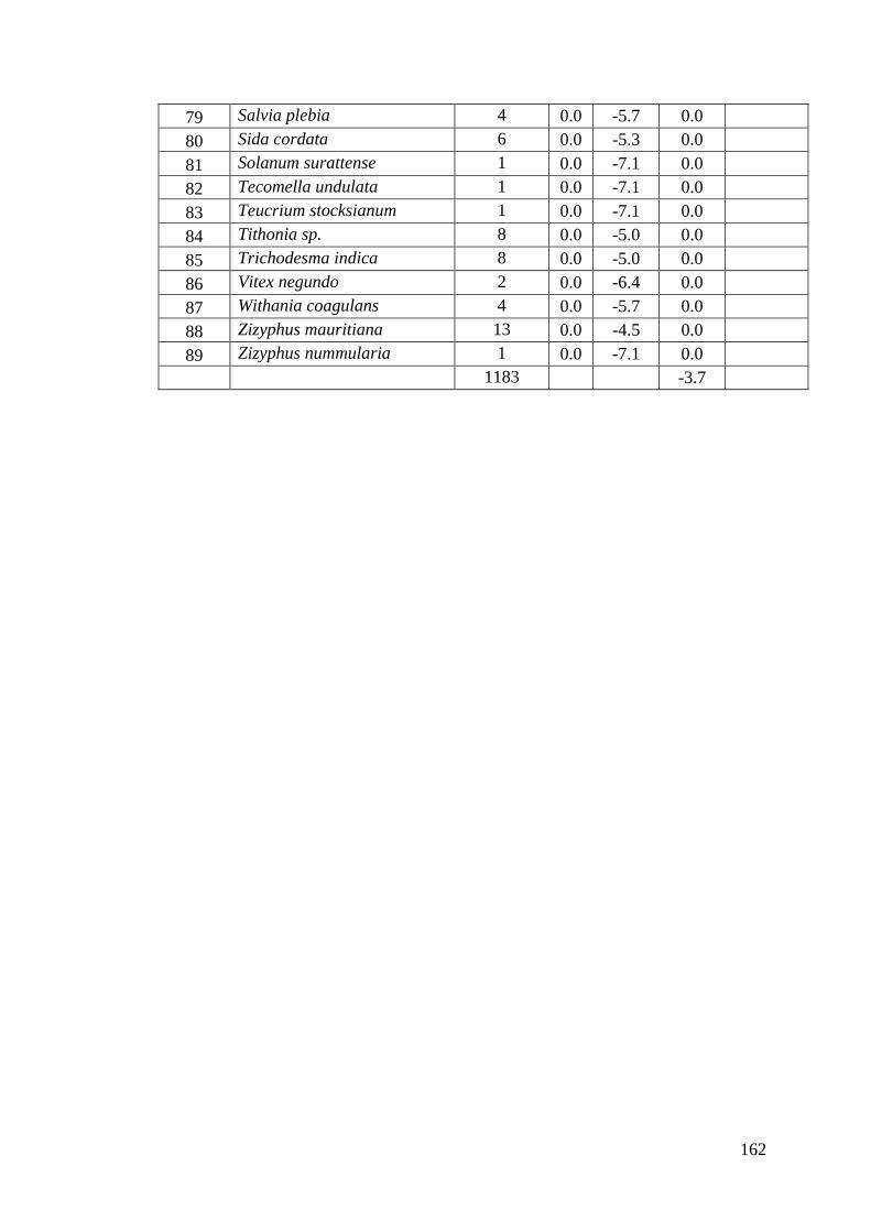
162
79 Salvia plebia 4 0.0 -5.7 0.0
80 Sida cordata 6 0.0 -5.3 0.0
81 Solanum surattense 1 0.0 -7.1 0.0
82 Tecomella undulata 1 0.0 -7.1 0.0
83 Teucrium stocksianum 1 0.0 -7.1 0.0
84 Tithonia sp. 8 0.0 -5.0 0.0
85 Trichodesma indica 8 0.0 -5.0 0.0
86 Vitex negundo 2 0.0 -6.4 0.0
87 Withania coagulans 4 0.0 -5.7 0.0
88 Zizyphus mauritiana 13 0.0 -4.5 0.0
89 Zizyphus nummularia 1 0.0 -7.1 0.0
1183 -3.7
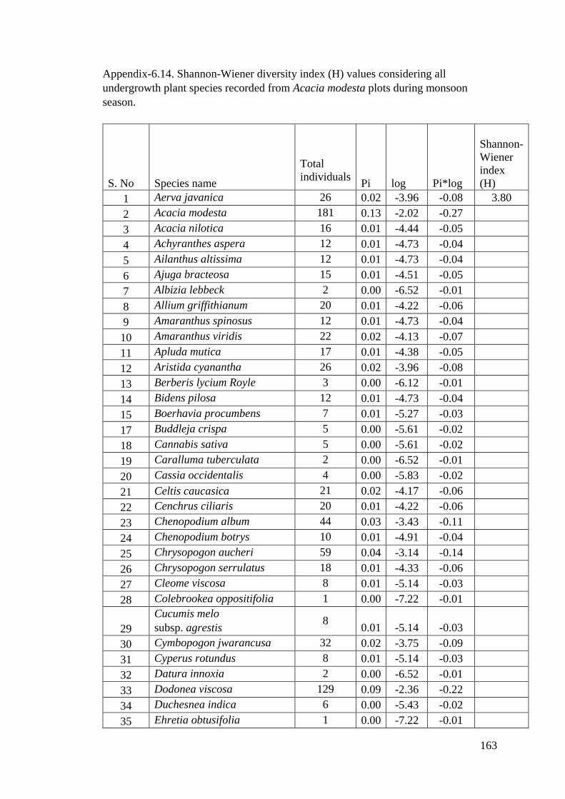
163
Appendix-6.14. Shannon-Wiener diversity index (H) values considering all
undergrowth plant species recorded from Acacia modesta plots during monsoon
season.
S. No Species name
Total
individuals Pi log Pi*log
Shannon-
Wiener
index
(H)
1 Aerva javanica 26 0.02 -3.96 -0.08 3.80
2 Acacia modesta 181 0.13 -2.02 -0.27
3 Acacia nilotica 16 0.01 -4.44 -0.05
4 Achyranthes aspera 12 0.01 -4.73 -0.04
5 Ailanthus altissima 12 0.01 -4.73 -0.04
6 Ajuga bracteosa 15 0.01 -4.51 -0.05
7 Albizia lebbeck 2 0.00 -6.52 -0.01
8 Allium griffithianum 20 0.01 -4.22 -0.06
9 Amaranthus spinosus 12 0.01 -4.73 -0.04
10 Amaranthus viridis 22 0.02 -4.13 -0.07
11 Apluda mutica 17 0.01 -4.38 -0.05
12 Aristida cyanantha 26 0.02 -3.96 -0.08
13 Berberis lycium Royle 3 0.00 -6.12 -0.01
14 Bidens pilosa 12 0.01 -4.73 -0.04
15 Boerhavia procumbens 7 0.01 -5.27 -0.03
17 Buddleja crispa 5 0.00 -5.61 -0.02
18 Cannabis sativa 5 0.00 -5.61 -0.02
19 Caralluma tuberculata 2 0.00 -6.52 -0.01
20 Cassia occidentalis 4 0.00 -5.83 -0.02
21 Celtis caucasica 21 0.02 -4.17 -0.06
22 Cenchrus ciliaris 20 0.01 -4.22 -0.06
23 Chenopodium album 44 0.03 -3.43 -0.11
24 Chenopodium botrys 10 0.01 -4.91 -0.04
25 Chrysopogon aucheri 59 0.04 -3.14 -0.14
26 Chrysopogon serrulatus 18 0.01 -4.33 -0.06
27 Cleome viscosa 8 0.01 -5.14 -0.03
28 Colebrookea oppositifolia 1 0.00 -7.22 -0.01
29
Cucumis melo
subsp. agrestis 8
0.01 -5.14 -0.03
30 Cymbopogon jwarancusa 32 0.02 -3.75 -0.09
31 Cyperus rotundus 8 0.01 -5.14 -0.03
32 Datura innoxia 2 0.00 -6.52 -0.01
33 Dodonea viscosa 129 0.09 -2.36 -0.22
34 Duchesnea indica 6 0.00 -5.43 -0.02
35 Ehretia obtusifolia 1 0.00 -7.22 -0.01

164
36 Eryngium biebersteinianum 2 0.00 -6.52 -0.01
37 Euphorbia hirta 8 0.01 -5.14 -0.03
38 Ficus palmata 26 0.02 -3.96 -0.08
39 Grevia optiva 28 0.02 -3.89 -0.08
40 Heliotropium strigosum 27 0.02 -3.92 -0.08
41 Herniaria hirsuta 17 0.01 -4.38 -0.05
42 Hyoscyamus niger 2 0.00 -6.52 -0.01
43 Justicia adhatoda 35 0.03 -3.66 -0.09
44 Kickxia ramosissima 13 0.01 -4.65 -0.04
45 Lamarckia aurea 29 0.02 -3.85 -0.08
46 Coronopus didymus 14 0.01 -4.58 -0.05
47 Lotus corniculatus 2 0.00 -6.52 -0.01
48 Mallotus philippensis 3 0.00 -6.12 -0.01
49 Martynia annua 4 0.00 -5.83 -0.02
50 Maytenus royleana 8 0.01 -5.14 -0.03
51 Melia azedarach 11 0.01 -4.82 -0.04
52 Melothria heterophylla 1 0.00 -7.22 -0.01
53 Mentha longifolia 1 0.00 -7.22 -0.01
54 Micromeria biflora 2 0.00 -6.52 -0.01
55 Monotheca buxifolia 1 0.00 -7.22 -0.01
56 Morus nigra 9 0.01 -5.02 -0.03
57 Myrsine africana 1 0.00 -7.22 -0.01
58 Nannorrhops ritchiana 2 0.00 -6.52 -0.01
59 Nerium odorum 2 0.00 -6.52 -0.01
60 Olea ferruginea 62 0.05 -3.09 -0.14
61 Onosma hispida 14 0.01 -4.58 -0.05
62 Otostegia limbata 22 0.02 -4.13 -0.07
63 Papaver pavoninum 4 0.00 -5.83 -0.02
64 Parthenium hysterophorus 13 0.01 -4.65 -0.04
65 Peganum harmala 4 0.00 -5.83 -0.02
66 Pennisetum flaccidum 8 0.01 -5.14 -0.03
67 Pentanema vestitum 25 0.02 -4.00 -0.07
68 Physalis divaricata 8 0.01 -5.14 -0.03
69 Plantago major 4 0.00 -5.83 -0.02
70 Isodon rugosus 2 0.00 -6.52 -0.01
71 Polygonum barbatum 14 0.01 -4.58 -0.05
72 Pupalia lappaceae 7 0.01 -5.27 -0.03
73 Rhazya stricta 2 0.00 -6.52 -0.01
74 Ricinus communis 3 0.00 -6.12 -0.01
75 Saccharum griffthii 21 0.02 -4.17 -0.06
76 Saccharum filifolium 39 0.03 -3.55 -0.10
77 Salvia lanata 5 0.00 -5.61 -0.02

165
78 salvia moorcroftiana 16 0.01 -4.44 -0.05
79 Salvia plebia 8 0.01 -5.14 -0.03
80 Sida cordata 6 0.00 -5.43 -0.02
81 Solanum surattense 1 0.00 -7.22 -0.01
82 Tecomella undulata 1 0.00 -7.22 -0.01
83 Teucrium stocksianum 1 0.00 -7.22 -0.01
84 Tithonia sp. 16 0.01 -4.44 -0.05
85 Trichodesma indica 16 0.01 -4.44 -0.05
86 Vitex negundo 4 0.00 -5.83 -0.02
87 Withania coagulans 5 0.00 -5.61 -0.02
88 Zizyphus mauritiana 16 0.01 -4.44 -0.05
89 Zizyphus nummularia 2 0.00 -6.52 -0.01
1363 -3.80

166
Appendix-6.15. Shannon-Wiener diversity index (H) values considering all
undergrowth plant species recorded from Acacia modesta plots during winter season.
S. No Species name
Total
individuals Pi log Pi*log
Shannon-
Wiener
index (H)
1 Aerva javanica 26 0.0 -3.7 -0.1 3.4
2 Acacia modesta 161 0.2 -1.8 -0.3
3 Acacia nilotica 13 0.0 -4.3 -0.1
4 Achyranthes aspera 12 0.0 -4.4 -0.1
5 Ailanthus altissima 10 0.0 -4.6 0.0
6 Ajuga bracteosa 15 0.0 -4.2 -0.1
7 Albizia lebbeck 2 0.0 -6.2 0.0
8 Allium griffithianum 20 0.0 -3.9 -0.1
9 Amaranthus spinosus 0 0.0 0.0 0.0
10 Amaranthus viridis 0 0.0 0.0 0.0
11 Apluda mutica 17 0.0 -4.1 -0.1
12 Aristida cyanantha 26 0.0 -3.7 -0.1
13 Berberis lycium 3 0.0 -5.8 0.0
14 Bidens pilosa 0 0.0 0.0 0.0
15 Boerhavia procumbens 7 0.0 -5.0 0.0
17 Buddleja crispa 5 0.0 -5.3 0.0
18 Cannabis sativa 5 0.0 -5.3 0.0
19 Caralluma tuberculata 2 0.0 -6.2 0.0
20 Cassia occidentalis 0 0.0 0.0 0.0
21 Celtis caucasica 15 0.0 -4.2 -0.1
22 Cenchrus ciliaris 20 0.0 -3.9 -0.1
23 Chenopodium album 0 0.0 0.0 0.0
24 Chenopodium botrys 10 0.0 -4.6 0.0
25 Chrysopogon aucheri 59 0.1 -2.8 -0.2
26 Chrysopogon serrulatus 18 0.0 -4.0 -0.1
27 Cleome viscosa 0 0.0 0.0 0.0
28 Colebrookea oppositifolia 1 0.0 -6.9 0.0
29
Cucumis melo
subsp. agrestis 4
0.0 -5.5 0.0
30 Cymbopogon jwarancusa 32 0.0 -3.4 -0.1
31 Cyperus rotundus 8 0.0 -4.8 0.0
32 Datura innoxia 2 0.0 -6.2 0.0
33 Dodonea viscosa 129 0.1 -2.1 -0.3
34 Duchesnea indica 6 0.0 -5.1 0.0
35 Ehretia obtusifolia 1 0.0 -6.9 0.0
36 Eryngium biebersteinianum 2 0.0 -6.2 0.0

167
37 Euphorbia hirta 0 0.0 0.0 0.0
38 Ficus palmata 22 0.0 -3.8 -0.1
39 Grevia optiva 26 0.0 -3.7 -0.1
40 Heliotropium strigosum 0 0.0 0.0 0.0
41 Herniaria hirsuta 0 0.0 0.0 0.0
42 Hyoscyamus niger 2 0.0 -6.2 0.0
43 Justicia adhatoda 35 0.0 -3.4 -0.1
44 Kickxia ramosissima 13 0.0 -4.3 -0.1
45 Lamarckia aurea 0 0.0 0.0 0.0
46 Coronopus didymus 0 0.0 0.0 0.0
47 Lotus corniculatus 2 0.0 -6.2 0.0
48 Mallotus philippensis 3 0.0 -5.8 0.0
49 Martynia annua 0 0.0 0.0 0.0
50 Maytenus royleana 8 0.0 -4.8 0.0
51 Melia azedarach 10 0.0 -4.6 0.0
52 Melothria heterophylla 1 0.0 -6.9 0.0
53 Mentha longifolia 1 0.0 -6.9 0.0
54 Micromeria biflora 2 0.0 -6.2 0.0
55 Monotheca buxifolia 1 0.0 -6.9 0.0
56 Morus nigra 7 0.0 -5.0 0.0
57 Myrsine africana 1 0.0 -6.9 0.0
58 Nannorrhops ritchiana 2 0.0 -6.2 0.0
59 Nerium odorum 2 0.0 -6.2 0.0
60 Olea ferruginea 57 0.1 -2.9 -0.2
61 Onosma hispida 14 0.0 -4.3 -0.1
62 Otostegia limbata 22 0.0 -3.8 -0.1
63 Papaver pavoninum 0 0.0 0.0 0.0
64 Parthenium hysterophorus 13 0.0 -4.3 -0.1
65 Peganum harmala 0 0.0 0.0 0.0
66 Pennisetum flaccidum 8 0.0 -4.8 0.0
67 Pentanema vestitum 0 0.0 0.0 0.0
68 Physalis divaricata 0 0.0 0.0 0.0
69 Plantago major 0 0.0 0.0 0.0
70 Isodon rugosus 2 0.0 -6.2 0.0
71 Polygonum barbatum 0 0.0 0.0 0.0
72 Pupalia lappaceae 7 0.0 -5.0 0.0
73 Rhazya stricta 2 0.0 -6.2 0.0
74 Ricinus communis 3 0.0 -5.8 0.0
75 Saccharum griffthii 21 0.0 -3.9 -0.1
76 Saccharum filifolium 39 0.0 -3.3 -0.1
77 Salvia lanata 5 0.0 -5.3 0.0
78 salvia moorcroftiana 16 0.0 -4.1 -0.1

168
79 Salvia plebia 0 0.0 0.0 0.0
80 Sida cordata 6 0.0 -5.1 0.0
81 Solanum surattense 1 0.0 -6.9 0.0
82 Tecomella undulata 1 0.0 -6.9 0.0
83 Teucrium stocksianum 1 0.0 -6.9 0.0
84 Tithonia sp. 0 0.0 0.0 0.0
85 Trichodesma indica 0 0.0 0.0 0.0
86 Vitex negundo 2 0.0 -6.2 0.0
87 Withania coagulans 4 0.0 -5.5 0.0
88 Zizyphus mauritiana 13 0.0 -4.3 -0.1
89 Zizyphus nummularia 1 0.0 -6.9 0.0
1007 -3.4

169
Appendix-6.16. Shannon-Wiener diversity index (H) values considering undergrowth
tree species only recorded from Acacia modesta plots during spring season.
S. No Species name
Total
individuals Pi log Pi*log
Shannon-
Wiener
index (H)
1 Acacia modesta 161 0.48 -0.74 -0.35 1.77
2 Acacia nilotica 13 0.04 -3.26 -0.13
3 Ailanthus altissima 10 0.03 -3.52 -0.10
4 Albizia lebbeck 2 0.01 -5.13 -0.03
5 Celtis caucasica 15 0.04 -3.11 -0.14
6 Ficus palmata 22 0.07 -2.73 -0.18
7 Grevia optiva 26 0.08 -2.56 -0.20
8 Melia azedarach 10 0.03 -3.52 -0.10
9 Monotheca buxifolia 1 0.00 -5.82 -0.02
10 Morus nigra 7 0.02 -3.88 -0.08
11 Olea ferruginea 57 0.17 -1.78 -0.30
12 Tecomella undulata 1 0.00 -5.82 -0.02
13 Zizyphus mauritiana 13 0.04 -3.26 -0.13
338 -1.77

170
Appendix-6.17. Shannon-Wiener diversity index (H) values considering undergrowth
tree species only recorded from Acacia modesta plots during monsoon season.
S. No Species name
Total
individuals Pi log Pi*log
Shannon-
Wiener
index
(H)
1 Acacia modesta 181 0.47 -0.76 -0.36 1.80
2 Acacia nilotica 16 0.04 -3.18 -0.13
3 Ailanthus altissima 12 0.03 -3.47 -0.11
4 Albizia lebbeck 2 0.01 -5.26 -0.03
5 Celtis caucasica 21 0.05 -2.91 -0.16
6 Ficus palmata 26 0.07 -2.70 -0.18
7 Grevia optiva 28 0.07 -2.62 -0.19
8 Melia azedarach 11 0.03 -3.56 -0.10
9 Monotheca buxifolia 1 0.00 -5.96 -0.02
10 Morus nigra 9 0.02 -3.76 -0.09
11 Olea ferruginea 62 0.16 -1.83 -0.29
12 Tecomella undulata 1 0.00 -5.96 -0.02
13 Zizyphus mauritiana 16 0.04 -3.18 -0.13
386 -1.80

171
Appendix-6.18. Shannon-Wiener diversity index (H) values considering undergrowth
tree species only recorded from Acacia modesta plots during winter season.
S. No Species name
Total
individuals Pi log Pi*log
Shannon-
Wiener
index (H)
1 Acacia modesta 161 0.48 -0.74 -0.35 1.77
2 Acacia nilotica 13 0.04 -3.26 -0.13
3 Ailanthus altissima 10 0.03 -3.52 -0.10
4 Albizia lebbeck 2 0.01 -5.13 -0.03
5 Celtis caucasica 15 0.04 -3.11 -0.14
6 Ficus palmata 22 0.07 -2.73 -0.18
7 Grevia optiva 26 0.08 -2.56 -0.20
8 Melia azedarach 10 0.03 -3.52 -0.10
9 Monotheca buxifolia 1 0.00 -5.82 -0.02
10 Morus nigra 7 0.02 -3.88 -0.08
11 Olea ferruginea 57 0.17 -1.78 -0.30
12 Tecomella undulata 1 0.00 -5.82 -0.02
13 Zizyphus mauritiana 13 0.04 -3.26 -0.13
338 -1.77

172
Appendix-6.19. Shannon-Wiener diversity index (H) value considering all
undergrowth plant species recorded from R. pseudoacacia plots during spring season.
S. No Species name
Total
individuals Pi log Pi*log
Shannon-
Wiener
index
(H)
1 Aerva sanguinolenta 34 0.0 -3.5 -0.1 3.6
2 Ailanthus altissima 12 0.0 -4.5 0.0
3 Ajuga bracteosa 13 0.0 -4.4 -0.1
4 Alternanthera pungens 25 0.0 -3.8 -0.1
5 Ammi visnaga 2 0.0 -6.3 0.0
6 Apluda mutica 20 0.0 -4.0 -0.1
7 Artemisia scoparia 13 0.0 -4.4 -0.1
8 Avena fatua 18 0.0 -4.1 -0.1
9 Bidens pilosa 5 0.0 -5.4 0.0
10 Broussonetia papyrifera 29 0.0 -3.6 -0.1
11 Calistemin lanceolatus 1 0.0 -7.0 0.0
12 Commelina paludosa 23 0.0 -3.9 -0.1
13 Cannabis sativa 40 0.0 -3.3 -0.1
14 Carthamus lanatus 40 0.0 -3.3 -0.1
15 Carthamus oxycantha 15 0.0 -4.3 -0.1
16 Cassia occidentalis 5 0.0 -5.4 0.0
17 Chenopodium album 18 0.0 -4.1 -0.1
18 Chenopodium ambrosioides 12 0.0 -4.5 0.0
19 Chrysopogon aucheri 51 0.0 -3.1 -0.1
20 Convolvulus arvense 3 0.0 -5.9 0.0
21 Conyza Canadensis 18 0.0 -4.1 -0.1
22 Cucumis melo subsp. agrestis 2 0.0 -6.3 0.0
23 Cynodon dactylon 20 0.0 -4.0 -0.1
24 Cynoglossum lanceolatum 6 0.0 -5.2 0.0
25 Dalbergia sissoo 2 0.0 -6.3 0.0
26 Dodonea viscosa 92 0.1 -2.5 -0.2
27 Euphorbia granulate 15 0.0 -4.3 -0.1
28 Euphorbia hirta 36 0.0 -3.4 -0.1
29 Euphorbia indica 14 0.0 -4.4 -0.1
30 Ficus palmata 16 0.0 -4.2 -0.1
31 Heliotropium strigosum 4 0.0 -5.6 0.0
32 Heteropogan contortus 14 0.0 -4.4 -0.1
33 Kickxia ramosissima 2 0.0 -6.3 0.0
34 Lathyrus cicera 5 0.0 -5.4 0.0
35 Launaea procumbens 13 0.0 -4.4 -0.1
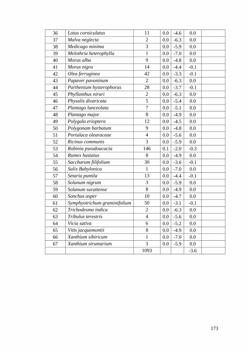
173
36 Lotus corniculatus 11 0.0 -4.6 0.0
37 Malva neglecta 2 0.0 -6.3 0.0
38 Medicago minima 3 0.0 -5.9 0.0
39 Melothria heterophylla 1 0.0 -7.0 0.0
40 Morus alba 9 0.0 -4.8 0.0
41 Morus nigra 14 0.0 -4.4 -0.1
42 Olea ferruginea 42 0.0 -3.3 -0.1
43 Papaver pavoninum 2 0.0 -6.3 0.0
44 Parthenium hysterophorus 28 0.0 -3.7 -0.1
45 Phyllanthus niruri 2 0.0 -6.3 0.0
46 Physalis divaricata 5 0.0 -5.4 0.0
47 Plantago lanceolata 7 0.0 -5.1 0.0
48 Plantago major 8 0.0 -4.9 0.0
49 Polygala erioptera 12 0.0 -4.5 0.0
50 Polygonam barbatum 9 0.0 -4.8 0.0
51 Portulaca olearaceae 4 0.0 -5.6 0.0
52 Ricinus communis 3 0.0 -5.9 0.0
53 Robinia pseudoacacia 146 0.1 -2.0 -0.3
54 Rumex hastatus 8 0.0 -4.9 0.0
55 Saccharum filifolium 30 0.0 -3.6 -0.1
56 Salix Babylonica 1 0.0 -7.0 0.0
57 Setaria pumila 13 0.0 -4.4 -0.1
58 Solanum nigrum 3 0.0 -5.9 0.0
59 Solanum surattense 8 0.0 -4.9 0.0
60 Sonchus asper 10 0.0 -4.7 0.0
61 Symphyotrichum graminifolium 50 0.0 -3.1 -0.1
62 Trichodesma indica 2 0.0 -6.3 0.0
63 Tribulus terestris 4 0.0 -5.6 0.0
64 Vicia sativa 6 0.0 -5.2 0.0
65 Vitis jacquemontii 8 0.0 -4.9 0.0
66 Xanthium sibiricum 1 0.0 -7.0 0.0
67 Xanthium strumarium 3 0.0 -5.9 0.0
1093 -3.6

174
Appendix-6.20. Shannon-Wiener diversity index (H) value considering all undergrowth
plant species recorded from R. pseudoacacia plots during monsoon season.
S. No Species name
Total
individuals Pi Log Pi*log
Shannon-
Wiener
index (H)
1 Aerva sanguinolenta 34 0.0 -3.7 -0.1 3.7
2 Ailanthus altissima 15 0.0 -4.5 -0.1
3 Ajuga bracteosa 13 0.0 -4.6 0.0
4 Alternanthera pungens 25 0.0 -4.0 -0.1
5 Ammi visnaga 4 0.0 -5.8 0.0
6 Apluda mutica L. 20 0.0 -4.2 -0.1
7 Artemisia scoparia 13 0.0 -4.6 0.0
8 Avena fatua 24 0.0 -4.0 -0.1
9 Bidens pilosa 9 0.0 -5.0 0.0
10 Broussonetia papyrifera 33 0.0 -3.7 -0.1
11 Calistemin lanceolatus 1 0.0 -7.2 0.0
12 Commelina paludosa 32 0.0 -3.7 -0.1
13 Cannabis sativa 40 0.0 -3.5 -0.1
14 Carthamus lanatus 57 0.0 -3.2 -0.1
15 Carthamus oxycantha 29 0.0 -3.8 -0.1
16 Cassia occidentalis 10 0.0 -4.9 0.0
17 Chenopodium album 36 0.0 -3.6 -0.1
18 Chenopodium ambrosioides 24 0.0 -4.0 -0.1
19 Chrysopogon aucheri 51 0.0 -3.3 -0.1
20 Convolvulus arvense 6 0.0 -5.4 0.0
21 Conyza Canadensis 34 0.0 -3.7 -0.1
22 Cucumis melo subsp. agrestis 4 0.0 -5.8 0.0
23 Cynodon dactylon 20 0.0 -4.2 -0.1
24 Cynoglossum lanceolatum 6 0.0 -5.4 0.0
25 Dalbergia sissoo 2 0.0 -6.5 0.0
26 Dodonea viscosa 92 0.1 -2.7 -0.2
27 Euphorbia granulate 23 0.0 -4.1 -0.1
28 Euphorbia hirta 51 0.0 -3.3 -0.1
29 Euphorbia indica 14 0.0 -4.6 0.0
30 Ficus palmata 20 0.0 -4.2 -0.1
31 Heliotropium strigosum 6 0.0 -5.4 0.0
32 Heteropogan contortus 14 0.0 -4.6 0.0
33 Kickxia ramosissima 2 0.0 -6.5 0.0
34 Lathyrus cicera 8 0.0 -5.1 0.0
35 Launaea procumbens 13 0.0 -4.6 0.0
36 Lotus corniculatus 11 0.0 -4.8 0.0

175
37 Malva neglecta 4 0.0 -5.8 0.0
38 Medicago minima 4 0.0 -5.8 0.0
39 Melothria heterophylla 1 0.0 -7.2 0.0
40 Morus alba 9 0.0 -5.0 0.0
41 Morus nigra 16 0.0 -4.4 -0.1
42 Olea ferruginea 47 0.0 -3.3 -0.1
43 Papaver pavoninum 4 0.0 -5.8 0.0
44 Parthenium hysterophorus 28 0.0 -3.9 -0.1
45 Phyllanthus niruri 2 0.0 -6.5 0.0
46 Physalis divaricata 10 0.0 -4.9 0.0
47 Plantago lanceolata 11 0.0 -4.8 0.0
48 Plantago major 15 0.0 -4.5 -0.1
49 Polygala erioptera 12 0.0 -4.7 0.0
50 Polygonam barbatum 17 0.0 -4.4 -0.1
51 Portulaca olearaceae 8 0.0 -5.1 0.0
52 Ricinus communis 3 0.0 -6.1 0.0
53 Robinia pseudoacacia 150 0.1 -2.2 -0.2
54 Rumex hastatus 13 0.0 -4.6 0.0
55 Saccharum filifolium 30 0.0 -3.8 -0.1
56 Salix Babylonica 1 0.0 -7.2 0.0
57 Setaria pumila 25 0.0 -4.0 -0.1
58 Solanum nigrum 5 0.0 -5.6 0.0
59 Solanum surattense 8 0.0 -5.1 0.0
60 Sonchus asper 10 0.0 -4.9 0.0
61 Symphyotrichum graminifolium 61 0.0 -3.1 -0.1
62 Trichodesma indica 4 0.0 -5.8 0.0
63 Tribulus terestris 7 0.0 -5.2 0.0
64 Vicia sativa 12 0.0 -4.7 0.0
65 Vitis jacquemontii 8 0.0 -5.1 0.0
66 Xanthium sibiricum 4 0.0 -5.8 0.0
67 Xanthium strumarium 6 0.0 -5.4 0.0
1331 -3.7

176
Appendix-6.21. Shannon-Wiener diversity index (H) value considering all
undergrowth plant species recorded from R. pseudoacacia plots during winter season.
S. No Species name
Total
individuals Pi log Pi*log
Shannon-
Wiener
index (H)
1 Aerva sanguinolenta 34 0.0 -3.1 -0.1 3.0
2 Ailanthus altissima 12 0.0 -4.1 -0.1
3 Ajuga bracteosa 13 0.0 -4.0 -0.1
4 Alternanthera pungens 25 0.0 -3.4 -0.1
5 Ammi visnaga 0 0.0 0.0 0.0
6 Apluda mutica 20 0.0 -3.6 -0.1
7 Artemisia scoparia 13 0.0 -4.0 -0.1
8 Avena fatua 0 0.0 0.0 0.0
9 Bidens pilosa 0 0.0 0.0 0.0
10 Broussonetia papyrifera 29 0.0 -3.2 -0.1
11 Calistemin lanceolatus 1 0.0 -6.6 0.0
12 Commelina paludosa 0 0.0 0.0 0.0
13 Cannabis sativa 40 0.1 -2.9 -0.2
14 Carthamus lanatus 0 0.0 0.0 0.0
15 Carthamus oxycantha 0 0.0 0.0 0.0
16 Cassia occidentalis 0 0.0 0.0 0.0
17 Chenopodium album 0 0.0 0.0 0.0
18 Chenopodium ambrosioides 0 0.0 0.0 0.0
19 Chrysopogon aucheri 51 0.1 -2.7 -0.2
20 Convolvulus arvense 0 0.0 0.0 0.0
21 Conyza Canadensis 0 0.0 0.0 0.0
22 Cucumis melo subsp. agrestis 0 0.0 0.0 0.0
23 Cynodon dactylon 20 0.0 -3.6 -0.1
24 Cynoglossum lanceolatum 6 0.0 -4.8 0.0
25 Dalbergia sissoo 2 0.0 -5.9 0.0
26 Dodonea viscosa 92 0.1 -2.1 -0.3
27 Euphorbia granulata 0 0.0 0.0 0.0
28 Euphorbia hirta 0 0.0 0.0 0.0
29 Euphorbia indica 0 0.0 0.0 0.0
30 Ficus palmata 16 0.0 -3.8 -0.1
31 Heliotropium strigosum 0 0.0 0.0 0.0
32 Heteropogan contortus 14 0.0 -4.0 -0.1
33 Kickxia ramosissima 2 0.0 -5.9 0.0
34 Lathyrus cicera 0 0.0 0.0 0.0
35 Launaea procumbens 13 0.0 -4.0 -0.1
36 Lotus corniculatus 11 0.0 -4.2 -0.1

177
37 Malva neglecta 0 0.0 0.0 0.0
38 Medicago minima 0 0.0 0.0 0.0
39 Melothria heterophylla 1 0.0 -6.6 0.0
40 Morus alba 9 0.0 -4.4 -0.1
41 Morus nigra 14 0.0 -4.0 -0.1
42 Olea ferruginea 42 0.1 -2.9 -0.2
43 Papaver pavoninum 0 0.0 0.0 0.0
44 Parthenium hysterophorus 28 0.0 -3.3 -0.1
45 Phyllanthus niruri 2 0.0 -5.9 0.0
46 Physalis divaricata 0 0.0 0.0 0.0
47 Plantago lanceolata 0 0.0 0.0 0.0
48 Plantago major 0 0.0 0.0 0.0
49 Polygala erioptera 12 0.0 -4.1 -0.1
50 Polygonam barbatum 0 0.0 0.0 0.0
51 Portulaca olearaceae 0 0.0 0.0 0.0
52 Ricinus communis 3 0.0 -5.5 0.0
53 Robinia pseudoacacia 146 0.2 -1.6 -0.3
54 Rumex hastatus 8 0.0 -4.5 0.0
55 Saccharum filifolium 30 0.0 -3.2 -0.1
56 Salix Babylonica 1 0.0 -6.6 0.0
57 Setaria pumila 0 0.0 0.0 0.0
58 Solanum nigrum 0 0.0 0.0 0.0
59 Solanum surattense 8 0.0 -4.5 0.0
60 Sonchus asper 10 0.0 -4.3 -0.1
61 Symphyotrichum graminifolium 0 0.0 0.0 0.0
62 Trichodesma indica 0 0.0 0.0 0.0
63 Tribulus terestris 0 0.0 0.0 0.0
64 Vicia sativa 0 0.0 0.0 0.0
65 Vitis jacquemontii 8 0.0 -4.5 0.0
66 Xanthium sibiricum 0 0.0 0.0 0.0
67 Xanthium strumarium 0 0.0 0.0 0.0
736 -3.0

178
Appendix-6.22. Shannon-Wiener diversity index (H) values considering undergrowth
tree species only recorded from R. pseudoacacia plots during spring season.
S. No Species name
Total
individuals Pi log Pi*log
Shannon-
Wiener
index (H)
1 Ailanthus altissima 12 0.0 -3.1 -0.1 1.5
2 Broussonetia papyrifera 29 0.1 -2.2 -0.2
3 Calistemin lanceolatus 1 0.0 -5.6 0.0
4 Dalbergia sissoo 2 0.0 -4.9 0.0
5 Ficus palmata 16 0.1 -2.8 -0.2
6 Morus alba 9 0.0 -3.4 -0.1
7 Morus nigra 14 0.1 -3.0 -0.2
8 Olea ferruginea 42 0.2 -1.9 -0.3
9 Robinia pseudoacacia 146 0.5 -0.6 -0.3
10 Salix Babylonica 1 0.0 -5.6 0.0
272 -1.5

179
Appendix- 6.23. Shannon-Wiener diversity index (H) values considering undergrowth
tree species only recorded from R. pseudoacacia plots during monsoon season.
S. No Species name
Total
individuals Pi log Pi*log
Shannon-
Wiener
index (H)
1 Ailanthus altissima 15 0.05 -2.98 -0.15 1.55
2 Broussonetia papyrifera 33 0.11 -2.19 -0.25
3 Calistemin lanceolatus 1 0.00 -5.68 -0.02
4 Dalbergia sissoo 2 0.01 -4.99 -0.03
5 Ficus palmata 20 0.07 -2.69 -0.18
6 Morus alba 9 0.03 -3.49 -0.11
7 Morus nigra 16 0.05 -2.91 -0.16
8 Olea ferruginea 47 0.16 -1.83 -0.29
9 Robinia pseudoacacia 150 0.51 -0.67 -0.34
10 Salix Babylonica 1 0.00 -5.68 -0.02
294 -1.55

180
Appendix-6.24. Shannon-Wiener diversity index (H) values considering undergrowth
tree species only recorded from R. pseudoacacia plots during winter season.
S. No Species name
Total
individuals Pi log Pi*log
Shannon-
Wiener
index
(H)
1 Ailanthus altissima 12 0.0 -3.1 -0.1 1.5
2 Broussonetia papyrifera 29 0.1 -2.2 -0.2
3 Calistemin lanceolatus 1 0.0 -5.6 0.0
4 Dalbergia sissoo 2 0.0 -4.9 0.0
5 Ficus palmata 16 0.1 -2.8 -0.2
6 Morus alba 9 0.0 -3.4 -0.1
7 Morus nigra 14 0.1 -3.0 -0.2
8 Olea ferruginea 42 0.2 -1.9 -0.3
9 Robinia pseudoacacia 146 0.5 -0.6 -0.3
10 Salix Babylonica 1 0.0 -5.6 0.0
272 -1.5

181
Appendix-6.25 Anova results for comparison of SWDI (H) values of all research plots
considering all undergrowth.
Statistix 8.1
Analysis of Variance Table for Data
Source DF SS MS F P
Plants 3 0.36250 0.12083 7.25 0.0202
Season 2 0.38000 0.19000 11.40 0.0090
Error 6 0.10000 0.01667
Total 11 0.84250
Grand Mean 3.5750 CV 3.61
Tukey's 1 Degree of Freedom Test for Nonadditivity
Source DF SS MS F P
Nonadditivity 1 0.00009 0.00009 0.00 0.9499
Remainder 5 0.09991 0.01998
Statistix 8.1
LSD All-Pairwise Comparisons Test of Data for Plants
Plants Mean Homogeneous Groups
1 3.8333 A
2 3.6333 AB
4 3.4333 B
3 3.4000 B
Alpha 0.05 Standard Error for Comparison 0.1054
Critical T Value 2.447 Critical Value for Comparison 0.2579
Error term used: Plants*Season, 6 DF
There are 2 groups (A and B) in which the means
are not significantly different from one another.
LSD All-Pairwise Comparisons Test of Data for Season
Season Mean Homogeneous Groups
2 3.7250 A
1 3.6750 A
3 3.3250 B
Alpha 0.05 Standard Error for Comparison 0.0913
Critical T Value 2.447 Critical Value for Comparison 0.2234
Error term used: Plants*Season, 6 DF
There are 2 groups (A and B) in which the means
are not significantly different from one another.

182
Appendix-6.26 Anova results for comparison of SWDI (H) values of all research plots
considering only trees species as undergrowth.
Statistix 8.1
Analysis of Variance Table for Data
Source DF SS MS F P
Plants 3 0.37792 0.12597 848.74 0.0000
Season 2 0.00241 0.00121 8.13 0.0196
Error 6 0.00089 0.00015
Total 11 0.38123
Grand Mean 1.7617 CV 0.69
Tukey's 1 Degree of Freedom Test for Nonadditivity
Source DF SS MS F P
Nonadditivity 1 8.341E-04 8.341E-04 73.92 0.0004
Remainder 5 5.642E-05 1.128E-05
Statistix 8.1 SWDI Considering Tree species
LSD All-Pairwise Comparisons Test of Data for Plants
Plants Mean Homogeneous Groups
1 2.0162 A
2 1.7805 B
3 1.7333 C
4 1.5167 D
Alpha 0.05 Standard Error for Comparison 9.947E-03
Critical T Value 2.447 Critical Value for Comparison 0.0243
Error term used: Plants*Season, 6 DF
All 4 means are significantly different from one another.
LSD All-Pairwise Comparisons Test of Data for Season
Season Mean Homogeneous Groups
2 1.7817 A
1 1.7517 B
3 1.7517 B
Alpha 0.05 Standard Error for Comparison 8.615E-03
Critical T Value 2.447 Critical Value for Comparison 0.0211
Error term used: Plants*Season, 6 DF
There are 2 groups (A and B) in which the means
are not significantly different from one another.

183
Appendix-6.27 Anova results for comparison of SWDI (H) values B/w exotic and
indigenous research plots considering all undergrowth.
Statistix 8.1
Analysis of Variance Table for Data
Source DF SS MS F P
Plants 1 0.15042 0.15042 90.25 0.0109
Season 2 0.19000 0.09500 57.00 0.0172
Error 2 0.00333 0.00167
Total 5 0.34375
Grand Mean 3.5750 CV 1.14
Tukey's 1 Degree of Freedom Test for Nonadditivity
Source DF SS MS F P
Nonadditivity 1 0.00053 0.00053 0.19 0.7399
Remainder 1 0.00281 0.00281
Statistix 8.1 , 31/12/2018, 21:56:58
LSD All-Pairwise Comparisons Test of Data for Plants
Plants Mean Homogeneous Groups
Indigenous 3.7333 A
Exotic 3.4167 B
Alpha 0.05 Standard Error for Comparison 0.0333
Critical T Value 4.303 Critical Value for Comparison 0.1434
Error term used: Plants*Season, 2 DF
All 2 means are significantly different from one another.
LSD All-Pairwise Comparisons Test of Data for Season
Season Mean Homogeneous Groups
Monsoon 3.7250 A
Spring 3.6750 A
Winter 3.3250 B
Alpha 0.05 Standard Error for Comparison 0.0408
Critical T Value 4.303 Critical Value for Comparison 0.1757
Error term used: Plants*Season, 2 DF
There are 2 groups (A and B) in which the means
are not significantly different from one another.

184
Appendix 6.28 Anova results for comparison of SWDI (H) values B/w exotic and
indigenous research plots considering only tree species as undergrowth.
Statistix 8.1
Analysis of Variance Table for Data
Source DF SS MS F P
Plants 1 0.11207 0.11207 517.23 0.0019
Season 2 0.00070 0.00035 1.62 0.3824
Error 2 0.00043 0.00022
Total 5 0.11320
Grand Mean 1.7600 CV 0.84
Tukey's 1 Degree of Freedom Test for Nonadditivity
Source DF SS MS F P
Nonadditivity 1 3.571E-04 3.571E-04 4.69 0.2755
Remainder 1 7.619E-05 7.619E-05
Statistix 8.1 SWDI for only trees species
LSD All-Pairwise Comparisons Test of Data for Plants
Plants Mean Homogeneous Groups
Indigenous plots 1.8967 A
Exotic Plots 1.6233 B
Alpha 0.05 Standard Error for Comparison 0.0120
Critical T Value 4.303 Critical Value for Comparison 0.0517
Error term used: Plants*Season, 2 DF
All 2 means are significantly different from one another.
LSD All-Pairwise Comparisons Test of Data for Season
Season Mean Homogeneous Groups
Monsoon 1.7750 A
Spring 1.7550 B
Winter 1.7500 A
Alpha 0.05 Standard Error for Comparison 0.0147
Critical T Value 4.303 Critical Value for Comparison 0.0633
Error term used: Plants*Season, 2 DF
There are no significant pairwise differences among the means.

185
Appendix-7.1 Different soil parameters recorded from exotic and indigenous tree plots during winter season 2017.
Plot Type Location Replication Organic
matter (%)
pH EC
dS/m
Organic
Carbon
(%)
Total
Nitrogen
(%)
Phosphorus
(ppm)
Potassium
(ppm)
CaCO3
(mmole/meter)
R. pseudoacacia 1 1 1.18 7.1 0.2 0.68 0.07 6.84 82.06 5.4
R. pseudoacacia 1 2 1.19 7.05 0.2 0.69 0.07 6.9 82.75 4.9
R. pseudoacacia 1 3 1.19 7.03 0.9 0.69 0.07 6.88 82.55 5.4
R. pseudoacacia 2 1 1.28 6.95 0.2 0.74 0.07 7.44 89.23 4.5
R. pseudoacacia 2 2 1.27 6.97 0.2 0.74 0.07 7.36 88.32 4.2
R. pseudoacacia 2 3 1.28 6.94 0.2 0.74 0.07 7.42 89.02 3.9
R. pseudoacacia 3 1 1.37 6.9 0.2 0.79 0.08 7.94 95.28 3.6
R. pseudoacacia 3 2 1.39 6.87 0.2 0.81 0.08 8.06 96.67 3.8
R. pseudoacacia 3 3 1.37 6.86 0.2 0.8 0.08 7.96 95.49 3.5
E. camaldulensis 1 1 1.16 7.2 0.2 0.67 0.07 6.73 80.74 6.1
E. camaldulensis 1 2 1.17 7.19 0.2 0.68 0.07 6.8 81.57 6.2
E. camaldulensis 1 3 1.15 7.1 0.2 0.67 0.07 6.68 80.18 6.1
E. camaldulensis 2 1 1.19 7.03 0.2 0.69 0.07 6.88 82.55 5.7
E. camaldulensis 2 2 1.19 7.05 0.1 0.69 0.07 6.9 82.82 5.7
E. camaldulensis 2 3 1.27 7.01 0.1 0.74 0.07 7.36 88.32 5.8
E. camaldulensis 3 1 1.29 6.99 0.1 0.75 0.07 7.48 89.71 3.8
E. camaldulensis 3 2 1.28 6.98 0.1 0.74 0.07 7.44 89.23 3.6
E. camaldulensis 3 3 1.29 6.96 0.1 0.75 0.07 7.48 89.71 3.6
Acacia modesta 1 1 1.17 6.99 0.2 0.68 0.07 6.8 81.57 5.9
Acacia modesta 1 2 1.19 6.96 0.1 0.69 0.07 6.88 82.55 5.9
Acacia modesta 1 3 1.2 6.97 0.2 0.69 0.07 6.94 83.33 5.7
Acacia modesta 2 1 1.38 6.94 0.1 0.8 0.08 8.02 96.19 4.7

186
Acacia modesta 2 2 1.39 6.94 0.1 0.81 0.08 8.05 96.6 5.1
Acacia modesta 2 3 1.38 6.92 0.1 0.8 0.08 8 95.98 5.1
Acacia modesta 3 1 1.47 6.87 0.1 0.85 0.09 8.54 102.45 3.1
Acacia modesta 3 2 1.49 6.89 0.1 0.86 0.09 8.64 103.63 3.3
Acacia modesta 3 3 1.48 6.85 0.1 0.86 0.09 8.58 102.94 3.3
Pinus roxburghii 1 1 1.75 6.87 0.1 1.02 0.1 10.15 121.8 3.4
Pinus roxburghii 1 2 1.79 6.83 0.1 1.04 0.1 10.37 124.44 3.7
Pinus roxburghii 1 3 1.78 6.8 0.1 1.03 0.1 10.34 124.03 3.4
Pinus roxburghii 2 1 1.79 6.78 0.1 1.04 0.1 10.38 124.58 2.8
Pinus roxburghii 2 2 1.82 6.8 0.1 1.06 0.11 10.56 126.67 2.9
Pinus roxburghii 2 3 1.82 6.76 0.1 1.06 0.11 10.56 126.67 2.9
Pinus roxburghii 3 1 1.98 6.73 0.1 1.15 0.11 11.46 137.46 2.3
Pinus roxburghii 3 2 1.97 6.73 0.1 1.14 0.11 11.44 137.25 2.2
Pinus roxburghii 3 3 1.98 6.7 0.1 1.15 0.12 11.5 137.95 2.5
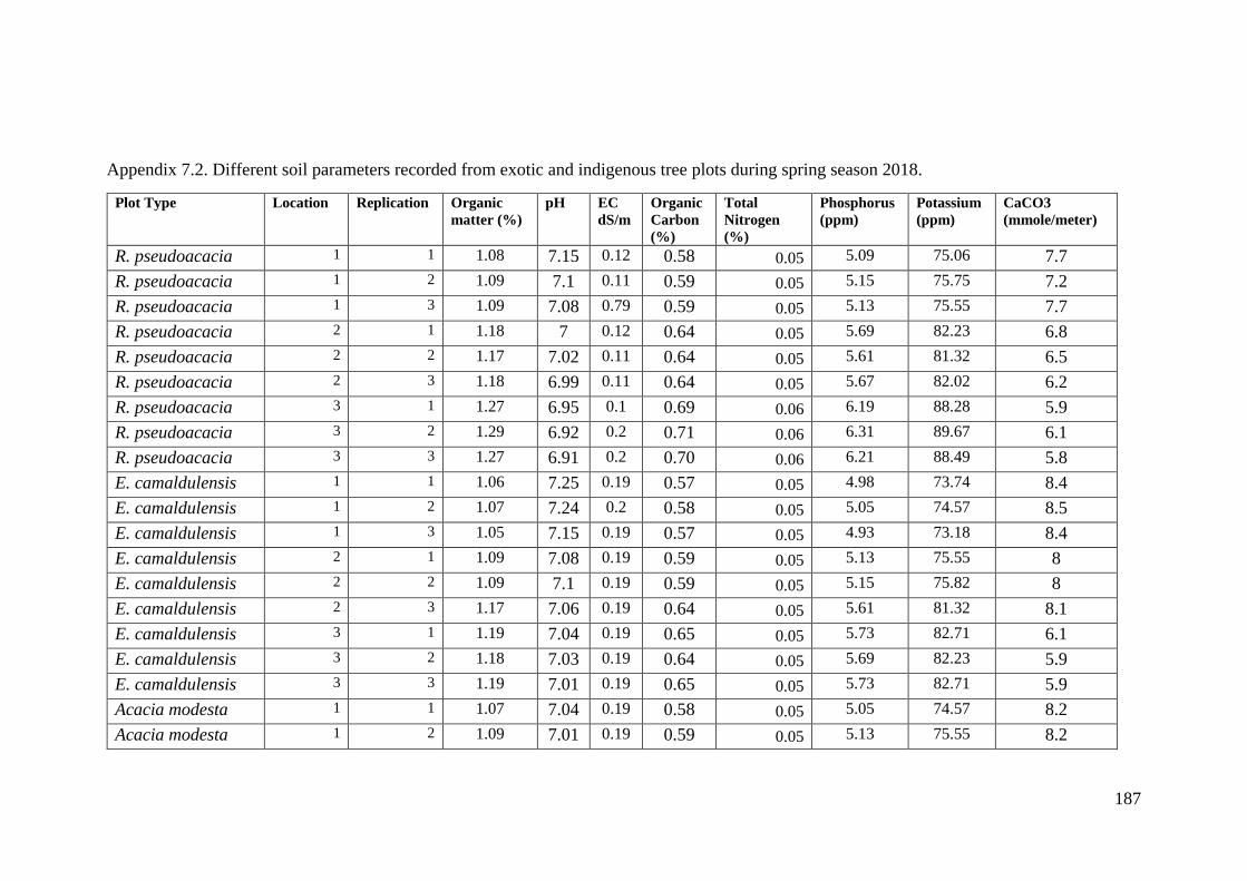
187
Appendix 7.2. Different soil parameters recorded from exotic and indigenous tree plots during spring season 2018.
Plot Type Location Replication Organic
matter (%)
pH EC
dS/m
Organic
Carbon
(%)
Total
Nitrogen
(%)
Phosphorus
(ppm)
Potassium
(ppm)
CaCO3
(mmole/meter)
R. pseudoacacia 1 1 1.08 7.15 0.12 0.58 0.05 5.09 75.06 7.7
R. pseudoacacia 1 2 1.09 7.1 0.11 0.59 0.05 5.15 75.75 7.2
R. pseudoacacia 1 3 1.09 7.08 0.79 0.59 0.05 5.13 75.55 7.7
R. pseudoacacia 2 1 1.18 7 0.12 0.64 0.05 5.69 82.23 6.8
R. pseudoacacia 2 2 1.17 7.02 0.11 0.64 0.05 5.61 81.32 6.5
R. pseudoacacia 2 3 1.18 6.99 0.11 0.64 0.05 5.67 82.02 6.2
R. pseudoacacia 3 1 1.27 6.95 0.1 0.69 0.06 6.19 88.28 5.9
R. pseudoacacia 3 2 1.29 6.92 0.2 0.71 0.06 6.31 89.67 6.1
R. pseudoacacia 3 3 1.27 6.91 0.2 0.70 0.06 6.21 88.49 5.8
E. camaldulensis 1 1 1.06 7.25 0.19 0.57 0.05 4.98 73.74 8.4
E. camaldulensis 1 2 1.07 7.24 0.2 0.58 0.05 5.05 74.57 8.5
E. camaldulensis 1 3 1.05 7.15 0.19 0.57 0.05 4.93 73.18 8.4
E. camaldulensis 2 1 1.09 7.08 0.19 0.59 0.05 5.13 75.55 8
E. camaldulensis 2 2 1.09 7.1 0.19 0.59 0.05 5.15 75.82 8
E. camaldulensis 2 3 1.17 7.06 0.19 0.64 0.05 5.61 81.32 8.1
E. camaldulensis 3 1 1.19 7.04 0.19 0.65 0.05 5.73 82.71 6.1
E. camaldulensis 3 2 1.18 7.03 0.19 0.64 0.05 5.69 82.23 5.9
E. camaldulensis 3 3 1.19 7.01 0.19 0.65 0.05 5.73 82.71 5.9
Acacia modesta 1 1 1.07 7.04 0.19 0.58 0.05 5.05 74.57 8.2
Acacia modesta 1 2 1.09 7.01 0.19 0.59 0.05 5.13 75.55 8.2

188
Acacia modesta 1 3 1.1 7.02 0.19 0.59 0.05 5.19 76.33 8
Acacia modesta 2 1 1.28 6.99 0.19 0.70 0.06 6.27 89.19 7
Acacia modesta 2 2 1.29 6.99 0.19 0.71 0.06 6.3 89.6 7.4
Acacia modesta 2 3 1.28 6.97 0.19 0.70 0.06 6.25 88.98 7.4
Acacia modesta 3 1 1.37 6.92 0.18 0.75 0.07 6.79 95.45 5.4
Acacia modesta 3 2 1.39 6.94 0.19 0.76 0.07 6.89 96.63 5.6
Acacia modesta 3 3 1.38 6.9 0.18 0.76 0.07 6.83 95.94 5.6
Pinus roxburghii 1 1 1.65 6.92 0.18 0.92 0.08 8.4 114.8 5.7
Pinus roxburghii 1 2 1.69 6.88 0.19 0.94 0.08 8.62 117.44 6
Pinus roxburghii 1 3 1.68 6.85 0.18 0.93 0.08 8.59 117.03 5.7
Pinus roxburghii 2 1 1.69 6.83 0.18 0.94 0.08 8.63 117.58 5.1
Pinus roxburghii 2 2 1.72 6.85 0.18 0.96 0.09 8.81 119.67 5.2
Pinus roxburghii 2 3 1.72 6.81 0.18 0.96 0.09 8.81 119.67 5.2
Pinus roxburghii 3 1 1.88 6.78 0.17 1.05 0.09 9.71 130.46 4.6
Pinus roxburghii 3 2 1.87 6.78 0.17 1.04 0.09 9.69 130.25 4.5
Pinus roxburghii 3 3 1.88 6.75 0.17 1.05 0.1 9.75 130.95 4.8

189
Appendix 7.3. Different soil parameters recorded from exotic and indigenous tree plots during monsoon season 2018.
Plot Type Location Replication Organic
matter (%)
pH EC
dS/m
Organic
Carbon
(%)
Total
Nitrogen
(%)
Phosphorus
(ppm)
Potassium
(ppm)
CaCO3
(mmole/meter)
R. pseudoacacia 1 1 1.48 7.07 0.16 0.76 0.1 8.79 93.06 4.7 R. pseudoacacia 1 2 1.49 7.02 0.15 0.77 0.1 8.85 93.75 4.2 R. pseudoacacia 1 3 1.49 7 0.83 0.77 0.1 8.83 93.55 4.7 R. pseudoacacia 2 1 1.58 6.92 0.16 0.82 0.1 9.39 100.23 3.8 R. pseudoacacia 2 2 1.57 6.94 0.15 0.82 0.1 9.31 99.32 3.5 R. pseudoacacia 2 3 1.58 6.91 0.15 0.82 0.1 9.37 100.02 3.2 R. pseudoacacia 3 1 1.67 6.87 0.14 0.87 0.11 9.89 106.28 2.9 R. pseudoacacia 3 2 1.69 6.84 0.14 0.89 0.11 10.01 107.67 3.1 R. pseudoacacia 3 3 1.67 6.83 0.14 0.88 0.11 9.91 106.49 2.8 E. camaldulensis 1 1 1.46 7.17 0.13 0.75 0.1 8.68 91.74 5.4 E. camaldulensis 1 2 1.47 7.16 0.14 0.76 0.1 8.75 92.57 5.5 E. camaldulensis 1 3 1.45 7.07 0.13 0.76 0.1 8.63 91.18 5.4 E. camaldulensis 2 1 1.49 7 0.13 0.77 0.1 8.83 93.55 5 E. camaldulensis 2 2 1.49 7.02 0.13 0.77 0.1 8.85 93.82 5 E. camaldulensis 2 3 1.47 6.98 0.13 0.82 0.1 9.31 99.32 5.1 E. camaldulensis 3 1 1.59 6.96 0.13 0.83 0.1 9.43 100.71 3.1 E. camaldulensis 3 2 1.58 6.95 0.13 0.82 0.1 9.39 100.23 2.9 E. camaldulensis 3 3 1.59 6.93 0.13 0.83 0.1 9.43 100.71 2.9 Acacia modesta 1 1 1.47 6.96 0.13 0.76 0.1 8.75 92.57 5.2 Acacia modesta 1 2 1.49 6.93 0.13 0.77 0.1 8.83 93.55 5.2 Acacia modesta 1 3 1.5 6.94 0.13 0.77 0.1 8.89 94.33 5 Acacia modesta 2 1 1.68 6.91 0.13 0.88 0.11 9.97 107.19 4

190
Acacia modesta 2 2 1.69 6.91 0.13 0.89 0.11 10 107.6 4.4 Acacia modesta 2 3 1.68 6.89 0.13 0.88 0.11 9.95 106.98 4.4 Acacia modesta 3 1 1.77 6.84 0.12 0.93 0.12 10.49 113.45 2.4 Acacia modesta 3 2 1.79 6.86 0.13 0.94 0.12 10.59 114.63 2.6 Acacia modesta 3 3 1.78 6.82 0.12 0.94 0.12 10.53 113.94 2.6 Pinus roxburghii 1 1 2.05 6.84 0.12 1.1 0.13 12.1 132.8 2.7 Pinus roxburghii 1 2 2.09 6.8 0.13 1.12 0.13 12.32 135.44 3 Pinus roxburghii 1 3 2.08 6.77 0.12 1.11 0.13 12.29 135.03 2.7 Pinus roxburghii 2 1 2.09 6.75 0.12 1.12 0.13 12.33 135.58 2.1 Pinus roxburghii 2 2 2.12 6.77 0.12 1.14 0.14 12.51 137.67 2.2 Pinus roxburghii 2 3 2.12 6.73 0.12 1.14 0.14 12.51 137.67 2.2 Pinus roxburghii 3 1 2.28 6.7 0.11 1.23 0.14 13.41 148.46 1.6 Pinus roxburghii 3 2 2.27 6.7 0.11 1.22 0.14 13.39 148.25 1.5 Pinus roxburghii 3 3 2.28 6.67 0.11 1.23 0.14 13.45 148.95 1.8

191
Appendix-8.
Statistix 8.1 Soil pH Analysis of Variance Table for Data
Source DF SS MS F P
Plants 3 1.08929 0.36310 522.86 0.0000
Location 2 0.38960 0.19480 280.51 0.0000
Season 2 0.11760 0.05880 84.67 0.0000
Plants*Location 6 0.03613 0.00602 8.67 0.0000
Plants*Season 6 9.324E-31 1.554E-31 0.00 1.0000
Location*Season 4 1.919E-30 4.798E-31 0.00 1.0000
Plants*Location*Season 12 2.465E-30 2.054E-31 0.00 1.0000
Error 72 0.05000 6.944E-04
Total 107 1.68263
Grand Mean 6.9375 CV 0.38
Statistix 8.1 Soil pH
LSD All-Pairwise Comparisons Test of Data for Plants
Plants Mean Homogeneous Groups
2 7.0633 A
1 6.9700 B
3 6.9322 C
4 6.7844 D
Alpha 0.05 Standard Error for Comparison 7.172E-03
Critical T Value 1.993 Critical Value for Comparison 0.0143
Error term used: Error, 72 DF
All 4 means are significantly different from one another.
LSD All-Pairwise Comparisons Test of Data for Location
Location Mean Homogeneous Groups
1 7.0142 A
2 6.9308 B
3 6.8675 C
Alpha 0.05 Standard Error for Comparison 6.211E-03
Critical T Value 1.993 Critical Value for Comparison 0.0124
Error term used: Error, 72 DF
All 3 means are significantly different from one another.
LSD All-Pairwise Comparisons Test of Data for Season
Season Mean Homogeneous Groups
2 6.9808 A
1 6.9308 B
3 6.9008 C
Alpha 0.05 Standard Error for Comparison 6.211E-03
Critical T Value 1.993 Critical Value for Comparison 0.0124
Error term used: Error, 72 DF
All 3 means are significantly different from one another.
LSD All-Pairwise Comparisons Test of Data for Plants*Location
Plants Location Mean Homogeneous Groups
2 1 7.1700 A
1 1 7.0667 B
2 2 7.0367 C
2 3 6.9833 D
3 1 6.9800 D
1 2 6.9600 DE
3 2 6.9400 E

192
1 3 6.8833 F
3 3 6.8767 F
4 1 6.8400 G
4 2 6.7867 H
4 3 6.7267 I
Alpha 0.05 Standard Error for Comparison 0.0124
Critical T Value 1.993 Critical Value for Comparison 0.0248
Error term used: Error, 72 DF
There are 9 groups (A, B, etc.) in which the means
are not significantly different from one another.
LSD All-Pairwise Comparisons Test of Data for Plants*Season
Plants Season Mean Homogeneous Groups
2 2 7.1067 A
2 1 7.0567 B
2 3 7.0267 C
1 2 7.0133 C
3 2 6.9756 D
1 1 6.9633 D
1 3 6.9333 E
3 1 6.9256 E
3 3 6.8956 F
4 2 6.8278 G
4 1 6.7778 H
4 3 6.7478 I
Alpha 0.05 Standard Error for Comparison 0.0124
Critical T Value 1.993 Critical Value for Comparison 0.0248
Error term used: Error, 72 DF
There are 9 groups (A, B, etc.) in which the means
are not significantly different from one another.
LSD All-Pairwise Comparisons Test of Data for Location*Season
Location Season Mean Homogeneous Groups
1 2 7.0575 A
1 1 7.0075 B
1 3 6.9775 C
2 2 6.9742 C
2 1 6.9242 D
3 2 6.9108 DE
2 3 6.8942 E
3 1 6.8608 F
3 3 6.8308 G
Alpha 0.05 Standard Error for Comparison 0.0108
Critical T Value 1.993 Critical Value for Comparison 0.0214
Error term used: Error, 72 DF
There are 7 groups (A, B, etc.) in which the means
are not significantly different from one another.
LSD All-Pairwise Comparisons Test of Data for Plants*Location*Season
Plants Location Season Mean Homogeneous Groups
2 1 2 7.2133 A
2 1 1 7.1633 B
2 1 3 7.1333 BC
1 1 2 7.1100 CD
2 2 2 7.0800 DE
1 1 1 7.0600 EF
1 1 3 7.0300 FG
2 2 1 7.0300 FG
2 3 2 7.0267 FG
3 1 2 7.0233 FGH
1 2 2 7.0033 GHI
2 2 3 7.0000 GHI

193
3 2 2 6.9833 HIJ
2 3 1 6.9767 IJ
3 1 1 6.9733 IJK
1 2 1 6.9533 JKL
2 3 3 6.9467 JKL
3 1 3 6.9433 JKLM
3 2 1 6.9333 KLM
1 3 2 6.9267 LM
1 2 3 6.9233 LMN
3 3 2 6.9200 LMN
3 2 3 6.9033 MNO
4 1 2 6.8833 NOP
1 3 1 6.8767 OPQ
3 3 1 6.8700 OPQR
1 3 3 6.8467 PQR
3 3 3 6.8400 QRS
4 1 1 6.8333 RS
4 2 2 6.8300 RS
4 1 3 6.8033 ST
4 2 1 6.7800 TU
4 3 2 6.7700 TU
4 2 3 6.7500 UV
4 3 1 6.7200 VW
4 3 3 6.6900 W
Alpha 0.05 Standard Error for Comparison 0.0215
Critical T Value 1.993 Critical Value for Comparison 0.0429
Error term used: Error, 72 DF
There are 23 groups (A, B, etc.) in which the means
are not significantly different from one another.

194
Appendix-9.
Statistix 8.1 Organic Matter
Analysis of Variance Table for Data
Source DF SS MS F P
Plants 3 6.8441 2.28138 9733.80 0.0000
Location 2 0.7504 0.37518 1600.75 0.0000
Season 2 3.0742 1.53709 6558.20 0.0000
Plants*Location 6 0.1063 0.01772 75.62 0.0000
Plants*Season 6 0.0005 0.00009 0.39 0.8849
Location*Season 4 0.0004 0.00009 0.40 0.8086
Plants*Location*Season 12 0.0011 0.00009 0.40 0.9595
Error 72 0.0169 0.00023
Total 107 10.7939
Grand Mean 1.4915 CV 1.03
Statistix 8.1 Organic Matter
LSD All-Pairwise Comparisons Test of Data for Plants
Plants Mean Homogeneous Groups
4 1.9199 A
3 1.4160 B
1 1.3460 C
2 1.2839 D
Alpha 0.05 Standard Error for Comparison 4.167E-03
Critical T Value 1.993 Critical Value for Comparison 8.306E-03
Error term used: Error, 72 DF
All 4 means are significantly different from one another.
LSD All-Pairwise Comparisons Test of Data for Location
Location Mean Homogeneous Groups
3 1.5966 A
2 1.4851 B
1 1.3927 C
Alpha 0.05 Standard Error for Comparison 3.608E-03
Critical T Value 1.993 Critical Value for Comparison 7.193E-03
Error term used: Error, 72 DF
All 3 means are significantly different from one another.
LSD All-Pairwise Comparisons Test of Data for Season
Season Mean Homogeneous Groups
3 1.7230 A
1 1.4257 B
2 1.3257 C
Alpha 0.05 Standard Error for Comparison 3.608E-03
Critical T Value 1.993 Critical Value for Comparison 7.193E-03
Error term used: Error, 72 DF
All 3 means are significantly different from one another.
LSD All-Pairwise Comparisons Test of Data for Plants*Location
Plants Location Mean Homogeneous Groups
4 3 2.0430 A
4 2 1.8767 B
4 1 1.8400 C
3 3 1.5467 D
3 2 1.4497 E
1 3 1.4433 E
2 3 1.3533 F

195
1 2 1.3433 F
2 2 1.2706 G
3 1 1.2517 H
1 1 1.2513 H
2 1 1.2278 I
Alpha 0.05 Standard Error for Comparison 7.217E-03
Critical T Value 1.993 Critical Value for Comparison 0.0144
Error term used: Error, 72 DF
There are 9 groups (A, B, etc.) in which the means
are not significantly different from one another.
LSD All-Pairwise Comparisons Test of Data for Plants*Season
Plants Season Mean Homogeneous Groups
4 3 2.1532 A
4 1 1.8532 B
4 2 1.7532 C
3 3 1.6494 D
1 3 1.5793 E
2 3 1.5099 F
3 1 1.3494 G
1 1 1.2793 H
3 2 1.2494 I
2 1 1.2210 J
1 2 1.1793 K
2 2 1.1208 L
Alpha 0.05 Standard Error for Comparison 7.217E-03
Critical T Value 1.993 Critical Value for Comparison 0.0144
Error term used: Error, 72 DF
All 12 means are significantly different from one another.
LSD All-Pairwise Comparisons Test of Data for Location*Season
Location Season Mean Homogeneous Groups
3 3 1.8299 A
2 3 1.7128 B
1 3 1.6261 C
3 1 1.5299 D
3 2 1.4299 E
2 1 1.4212 E
1 1 1.3261 F
2 2 1.3212 F
1 2 1.2259 G
Alpha 0.05 Standard Error for Comparison 6.250E-03
Critical T Value 1.993 Critical Value for Comparison 0.0125
Error term used: Error, 72 DF
There are 7 groups (A, B, etc.) in which the means
are not significantly different from one another.
LSD All-Pairwise Comparisons Test of Data for Plants*Location*Season
Plants Location Season Mean Homogeneous Groups
4 3 3 2.2763 A
4 2 3 2.1100 B
4 1 3 2.0733 C
4 3 1 1.9763 D
4 3 2 1.8763 E
4 2 1 1.8100 F
3 3 3 1.7800 G
4 1 1 1.7733 G
4 2 2 1.7100 H
3 2 3 1.6830 I
1 3 3 1.6767 I
4 1 2 1.6733 I
2 3 3 1.5867 J

196
1 2 3 1.5767 J
3 1 3 1.4851 K
1 1 3 1.4847 K
2 2 3 1.4817 K
3 3 1 1.4800 K
2 1 3 1.4613 K
3 2 1 1.3830 L
3 3 2 1.3800 L
1 3 1 1.3767 L
2 3 1 1.2867 M
3 2 2 1.2830 M
1 2 1 1.2767 M
1 3 2 1.2767 M
2 2 1 1.2150 N
2 3 2 1.1867 O
3 1 1 1.1851 OP
1 1 1 1.1847 OP
1 2 2 1.1767 OP
2 1 1 1.1613 P
2 2 2 1.1150 Q
3 1 2 1.0851 R
1 1 2 1.0847 R
2 1 2 1.0607 R
Alpha 0.05 Standard Error for Comparison 0.0125
Critical T Value 1.993 Critical Value for Comparison 0.0249
Error term used: Error, 72 DF
There are 18 groups (A, B, etc.) in which the means
are not significantly different from one another.

197
Appendix-10
Statistix 8.1 Organic carbon
Analysis of Variance Table for Data
Source DF SS MS F P
Plants 3 2.29942 0.76647 6979.06 0.0000
Location 2 0.25118 0.12559 1143.57 0.0000
Season 2 0.58336 0.29168 2655.86 0.0000
Plants*Location 6 0.03526 0.00588 53.51 0.0000
Plants*Season 6 0.00002 2.946E-06 0.03 0.9999
Location*Season 4 0.00002 4.893E-06 0.04 0.9962
Plants*Location*Season 12 0.00003 2.404E-06 0.02 1.0000
Error 72 0.00791 1.098E-04
Total 107 3.17719
Grand Mean 0.8207 CV 1.28
Statistix 8.1 Organic carbon
LSD All-Pairwise Comparisons Test of Data for Plants
Plants Mean Homogeneous Groups
4 1.0694 A
3 0.7757 B
1 0.7355 C
2 0.7023 D
Alpha 0.05 Standard Error for Comparison 2.852E-03
Critical T Value 1.993 Critical Value for Comparison 5.686E-03
Error term used: Error, 72 DF
All 4 means are significantly different from one another.
LSD All-Pairwise Comparisons Test of Data for Location
Location Mean Homogeneous Groups
3 0.8808 A
2 0.8186 B
1 0.7627 C
Alpha 0.05 Standard Error for Comparison 2.470E-03
Critical T Value 1.993 Critical Value for Comparison 4.924E-03
Error term used: Error, 72 DF
All 3 means are significantly different from one another.
LSD All-Pairwise Comparisons Test of Data for Season
Season Mean Homogeneous Groups
3 0.9071 A
1 0.8275 B
2 0.7275 C
Alpha 0.05 Standard Error for Comparison 2.470E-03
Critical T Value 1.993 Critical Value for Comparison 4.924E-03
Error term used: Error, 72 DF
All 3 means are significantly different from one another.
LSD All-Pairwise Comparisons Test of Data for Plants*Location
Plants Location Mean Homogeneous Groups
4 3 1.1399 A
4 2 1.0455 B
4 1 1.0228 C
3 3 0.8506 D
3 2 0.7963 E
1 3 0.7928 E
2 3 0.7399 F
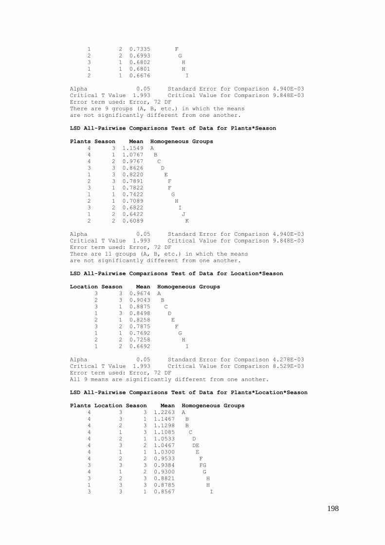
198
1 2 0.7335 F
2 2 0.6993 G
3 1 0.6802 H
1 1 0.6801 H
2 1 0.6676 I
Alpha 0.05 Standard Error for Comparison 4.940E-03
Critical T Value 1.993 Critical Value for Comparison 9.848E-03
Error term used: Error, 72 DF
There are 9 groups (A, B, etc.) in which the means
are not significantly different from one another.
LSD All-Pairwise Comparisons Test of Data for Plants*Season
Plants Season Mean Homogeneous Groups
4 3 1.1549 A
4 1 1.0767 B
4 2 0.9767 C
3 3 0.8626 D
1 3 0.8220 E
2 3 0.7891 F
3 1 0.7822 F
1 1 0.7422 G
2 1 0.7089 H
3 2 0.6822 I
1 2 0.6422 J
2 2 0.6089 K
Alpha 0.05 Standard Error for Comparison 4.940E-03
Critical T Value 1.993 Critical Value for Comparison 9.848E-03
Error term used: Error, 72 DF
There are 11 groups (A, B, etc.) in which the means
are not significantly different from one another.
LSD All-Pairwise Comparisons Test of Data for Location*Season
Location Season Mean Homogeneous Groups
3 3 0.9674 A
2 3 0.9043 B
3 1 0.8875 C
1 3 0.8498 D
2 1 0.8258 E
3 2 0.7875 F
1 1 0.7692 G
2 2 0.7258 H
1 2 0.6692 I
Alpha 0.05 Standard Error for Comparison 4.278E-03
Critical T Value 1.993 Critical Value for Comparison 8.529E-03
Error term used: Error, 72 DF
All 9 means are significantly different from one another.
LSD All-Pairwise Comparisons Test of Data for Plants*Location*Season
Plants Location Season Mean Homogeneous Groups
4 3 3 1.2263 A
4 3 1 1.1467 B
4 2 3 1.1298 B
4 1 3 1.1085 C
4 2 1 1.0533 D
4 3 2 1.0467 DE
4 1 1 1.0300 E
4 2 2 0.9533 F
3 3 3 0.9384 FG
4 1 2 0.9300 G
3 2 3 0.8821 H
1 3 3 0.8785 H
3 3 1 0.8567 I

199
2 3 3 0.8263 J
1 2 3 0.8205 J
3 2 1 0.8033 K
1 3 1 0.8000 KL
2 2 3 0.7847 L
3 1 3 0.7673 M
1 1 3 0.7671 M
3 3 2 0.7567 MN
2 1 3 0.7562 MN
2 3 1 0.7467 N
1 2 1 0.7400 N
2 2 1 0.7067 O
3 2 2 0.7033 OP
1 3 2 0.7000 OP
1 1 1 0.6867 PQ
3 1 1 0.6867 PQ
2 1 1 0.6733 Q
2 3 2 0.6467 R
1 2 2 0.6400 R
2 2 2 0.6067 S
1 1 2 0.5867 T
3 1 2 0.5867 T
2 1 2 0.5733 T
Alpha 0.05 Standard Error for Comparison 8.557E-03
Critical T Value 1.993 Critical Value for Comparison 0.0171
Error term used: Error, 72 DF
There are 20 groups (A, B, etc.) in which the means
are not significantly different from one another.

200
Appendix-11
Statistix 8.1 Electric conductivity
Analysis of Variance Table for Data
Source DF SS MS F P
Plants 3 0.10803 0.03601 2.82 0.0447
Location 2 0.09022 0.04511 3.54 0.0342
Season 2 0.02961 0.01480 1.16 0.3189
Plants*Location 6 0.21527 0.03588 2.81 0.0162
Plants*Season 6 0.02722 0.00454 0.36 0.9042
Location*Season 4 0.00148 0.00037 0.03 0.9983
Plants*Location*Season 12 0.00444 0.00037 0.03 1.0000
Error 72 0.91793 0.01275
Total 107 1.39421
Grand Mean 0.1692 CV 66.73
Statistix 8.1 Electric conductivity
LSD All-Pairwise Comparisons Test of Data for Plants
Plants Mean Homogeneous Groups
1 0.2233 A
2 0.1569 B
3 0.1534 B
4 0.1432 B
Alpha 0.05 Standard Error for Comparison 0.0307
Critical T Value 1.993 Critical Value for Comparison 0.0613
Error term used: Error, 72 DF
There are 2 groups (A and B) in which the means
are not significantly different from one another.
LSD All-Pairwise Comparisons Test of Data for Location
Location Mean Homogeneous Groups
1 0.2101 A
2 0.1493 B
3 0.1483 B
Alpha 0.05 Standard Error for Comparison 0.0266
Critical T Value 1.993 Critical Value for Comparison 0.0531
Error term used: Error, 72 DF
There are 2 groups (A and B) in which the means
are not significantly different from one another.
LSD All-Pairwise Comparisons Test of Data for Season
Season Mean Homogeneous Groups
2 0.1896 A
1 0.1690 A
3 0.1490 A
Alpha 0.05 Standard Error for Comparison 0.0266
Critical T Value 1.993 Critical Value for Comparison 0.0531
Error term used: Error, 72 DF
There are no significant pairwise differences among the means.
LSD All-Pairwise Comparisons Test of Data for Plants*Location
Plants Location Mean Homogeneous Groups
1 1 0.3733 A
2 1 0.1613 B
3 1 0.1567 B
2 2 0.1563 B

201
3 2 0.1543 B
1 3 0.1532 B
2 3 0.1530 B
3 3 0.1493 B
4 1 0.1490 B
1 2 0.1433 B
4 2 0.1430 B
4 3 0.1377 B
Alpha 0.05 Standard Error for Comparison 0.0532
Critical T Value 1.993 Critical Value for Comparison 0.1061
Error term used: Error, 72 DF
There are 2 groups (A and B) in which the means
are not significantly different from one another.
LSD All-Pairwise Comparisons Test of Data for Plants*Season
Plants Season Mean Homogeneous Groups
1 1 0.2426 A
1 3 0.2226 AB
1 2 0.2048 AB
2 2 0.1902 AB
3 2 0.1868 AB
4 2 0.1766 AB
2 1 0.1502 AB
3 1 0.1468 AB
4 1 0.1366 AB
2 3 0.1302 B
3 3 0.1268 B
4 3 0.1166 B
Alpha 0.05 Standard Error for Comparison 0.0532
Critical T Value 1.993 Critical Value for Comparison 0.1061
Error term used: Error, 72 DF
There are 2 groups (A and B) in which the means
are not significantly different from one another.
LSD All-Pairwise Comparisons Test of Data for Location*Season
Location Season Mean Homogeneous Groups
1 2 0.2268 A
1 1 0.2117 AB
1 3 0.1918 AB
3 2 0.1761 AB
2 2 0.1659 AB
2 1 0.1509 AB
3 1 0.1444 AB
2 3 0.1309 B
3 3 0.1244 B
Alpha 0.05 Standard Error for Comparison 0.0461
Critical T Value 1.993 Critical Value for Comparison 0.0919
Error term used: Error, 72 DF
There are 2 groups (A and B) in which the means
are not significantly different from one another.
LSD All-Pairwise Comparisons Test of Data for Plants*Location*Season
Plants Location Season Mean Homogeneous Groups
1 1 1 0.4000 A
1 1 3 0.3800 A
1 1 2 0.3400 AB
2 1 2 0.1947 BC
3 1 2 0.1900 BC
2 2 2 0.1897 BC
3 2 2 0.1877 BC
2 3 2 0.1863 BC
3 3 2 0.1827 BC

202
4 1 2 0.1823 BC
4 2 2 0.1763 BC
4 3 2 0.1710 BC
1 2 1 0.1700 BC
1 3 2 0.1643 BC
1 3 1 0.1577 BC
2 1 1 0.1547 C
1 2 3 0.1500 C
3 1 1 0.1500 C
2 2 1 0.1497 C
3 2 1 0.1477 C
2 3 1 0.1463 C
3 3 1 0.1427 C
4 1 1 0.1423 C
1 3 3 0.1377 C
4 2 1 0.1363 C
2 1 3 0.1347 C
4 3 1 0.1310 C
3 1 3 0.1300 C
2 2 3 0.1297 C
3 2 3 0.1277 C
2 3 3 0.1263 C
3 3 3 0.1227 C
4 1 3 0.1223 C
4 2 3 0.1163 C
4 3 3 0.1110 C
1 2 2 0.1100 C
Alpha 0.05 Standard Error for Comparison 0.0922
Critical T Value 1.993 Critical Value for Comparison 0.1838
Error term used: Error, 72 DF
There are 3 groups (A, B, etc.) in which the means
are not significantly different from one another.

203
Appendix-12
Statistix 8.1 Total Nitrogen
Analysis of Variance Table for Data
Source DF SS MS F P
Plants 3 0.02289 0.00763 7733.07 0.0000
Location 2 0.00253 0.00126 1279.73 0.0000
Season 2 0.04556 0.02278 23090.3 0.0000
Plants*Location 6 3.558E-04 5.930E-05 60.10 0.0000
Plants*Season 6 2.923E-10 4.871E-11 0.00 1.0000
Location*Season 4 1.782E-09 4.454E-10 0.00 1.0000
Plants*Location*Season 12 1.645E-09 1.371E-10 0.00 1.0000
Error 72 7.104E-05 9.866E-07
Total 107 0.07140
Grand Mean 0.0860 CV 1.15
Statistix 8.1 Total Nitrogen
LSD All-Pairwise Comparisons Test of Data for Plants
Plants Mean Homogeneous Groups
4 0.1108 A
3 0.0816 B
1 0.0775 C
2 0.0742 D
Alpha 0.05 Standard Error for Comparison 2.703E-04
Critical T Value 1.993 Critical Value for Comparison 5.389E-04
Error term used: Error, 72 DF
All 4 means are significantly different from one another.
LSD All-Pairwise Comparisons Test of Data for Location
Location Mean Homogeneous Groups
3 0.0921 A
2 0.0858 B
1 0.0803 C
Alpha 0.05 Standard Error for Comparison 2.341E-04
Critical T Value 1.993 Critical Value for Comparison 4.667E-04
Error term used: Error, 72 DF
All 3 means are significantly different from one another.
LSD All-Pairwise Comparisons Test of Data for Season
Season Mean Homogeneous Groups
3 0.1127 A
1 0.0827 B
2 0.0627 C
Alpha 0.05 Standard Error for Comparison 2.341E-04
Critical T Value 1.993 Critical Value for Comparison 4.667E-04
Error term used: Error, 72 DF
All 3 means are significantly different from one another.
LSD All-Pairwise Comparisons Test of Data for Plants*Location
Plants Location Mean Homogeneous Groups
4 3 0.1180 A
4 2 0.1083 B
4 1 0.1062 C
3 3 0.0892 D
3 2 0.0836 E
1 3 0.0832 E

204
2 3 0.0780 F
1 2 0.0774 F
2 2 0.0738 G
3 1 0.0721 H
1 1 0.0721 H
2 1 0.0707 I
Alpha 0.05 Standard Error for Comparison 4.682E-04
Critical T Value 1.993 Critical Value for Comparison 9.334E-04
Error term used: Error, 72 DF
There are 9 groups (A, B, etc.) in which the means
are not significantly different from one another.
LSD All-Pairwise Comparisons Test of Data for Plants*Season
Plants Season Mean Homogeneous Groups
4 3 0.1375 A
3 3 0.1083 B
4 1 0.1075 B
1 3 0.1042 C
2 3 0.1008 D
4 2 0.0875 E
3 1 0.0783 F
1 1 0.0742 G
2 1 0.0708 H
3 2 0.0583 I
1 2 0.0542 J
2 2 0.0508 K
Alpha 0.05 Standard Error for Comparison 4.682E-04
Critical T Value 1.993 Critical Value for Comparison 9.334E-04
Error term used: Error, 72 DF
There are 11 groups (A, B, etc.) in which the means
are not significantly different from one another.
LSD All-Pairwise Comparisons Test of Data for Location*Season
Location Season Mean Homogeneous Groups
3 3 0.1187 A
2 3 0.1124 B
1 3 0.1069 C
3 1 0.0888 D
2 1 0.0824 E
1 1 0.0769 F
3 2 0.0688 G
2 2 0.0624 H
1 2 0.0569 I
Alpha 0.05 Standard Error for Comparison 4.055E-04
Critical T Value 1.993 Critical Value for Comparison 8.084E-04
Error term used: Error, 72 DF
All 9 means are significantly different from one another.
LSD All-Pairwise Comparisons Test of Data for Plants*Location*Season
Plants Location Season Mean Homogeneous Groups
4 3 3 0.1446 A
4 2 3 0.1350 B
4 1 3 0.1329 C
3 3 3 0.1158 D
4 3 1 0.1147 D
3 2 3 0.1102 E
1 3 3 0.1098 E
4 2 1 0.1050 F
2 3 3 0.1046 F
1 2 3 0.1040 FG
4 1 1 0.1029 G
2 2 3 0.1005 H

205
3 1 3 0.0987 I
1 1 3 0.0987 I
2 1 3 0.0974 I
4 3 2 0.0947 J
3 3 1 0.0859 K
4 2 2 0.0850 K
4 1 2 0.0829 L
3 2 1 0.0802 M
1 3 1 0.0799 M
2 3 1 0.0747 N
1 2 1 0.0741 N
2 2 1 0.0705 O
1 1 1 0.0687 P
3 1 1 0.0687 P
2 1 1 0.0674 PQ
3 3 2 0.0659 Q
3 2 2 0.0602 R
1 3 2 0.0599 R
2 3 2 0.0547 S
1 2 2 0.0541 S
2 2 2 0.0505 T
1 1 2 0.0487 U
3 1 2 0.0487 U
2 1 2 0.0474 U
Alpha 0.05 Standard Error for Comparison 8.110E-04
Critical T Value 1.993 Critical Value for Comparison 1.617E-03
Error term used: Error, 72 DF
There are 21 groups (A, B, etc.) in which the means
are not significantly different from one another.

206
Appendix-13
Statistix 8.1 Phosphorus
Analysis of Variance Table for Data
Source DF SS MS F P
Plants 3 228.822 76.2740 7785.50 0.0000
Location 2 25.1918 12.5959 1285.70 0.0000
Season 2 246.660 123.330 12588.6 0.0000
Plants*Location 6 3.55473 0.59246 60.47 0.0000
Plants*Season 6 1.020E-30 1.701E-31 0.00 1.0000
Location*Season 4 3.325E-30 8.313E-31 0.00 1.0000
Plants*Location*Season 12 3.744E-30 3.120E-31 0.00 1.0000
Error 72 0.70538 0.00980
Total 107 504.934
Grand Mean 8.3359 CV 1.19
Statistix 8.1 Phosphorus
LSD All-Pairwise Comparisons Test of Data for Plants
Plants Mean Homogeneous Groups
4 10.815 A
3 7.893 B
1 7.487 C
2 7.148 D
Alpha 0.05 Standard Error for Comparison 0.0269
Critical T Value 1.993 Critical Value for Comparison 0.0537
Error term used: Error, 72 DF
All 4 means are significantly different from one another.
LSD All-Pairwise Comparisons Test of Data for Location
Location Mean Homogeneous Groups
3 8.9402 A
2 8.3094 B
1 7.7580 C
Alpha 0.05 Standard Error for Comparison 0.0233
Critical T Value 1.993 Critical Value for Comparison 0.0465
Error term used: Error, 72 DF
All 3 means are significantly different from one another.
LSD All-Pairwise Comparisons Test of Data for Season
Season Mean Homogeneous Groups
3 10.219 A
1 8.269 B
2 6.519 C
Alpha 0.05 Standard Error for Comparison 0.0233
Critical T Value 1.993 Critical Value for Comparison 0.0465
Error term used: Error, 72 DF
All 3 means are significantly different from one another.
LSD All-Pairwise Comparisons Test of Data for Plants*Location
Plants Location Mean Homogeneous Groups
4 3 11.529 A
4 2 10.565 B
4 1 10.352 C
3 3 8.651 D
3 2 8.088 E
1 3 8.051 E

207
2 3 7.529 F
1 2 7.471 F
2 2 7.114 G
3 1 6.940 H
1 1 6.938 H
2 1 6.802 I
Alpha 0.05 Standard Error for Comparison 0.0467
Critical T Value 1.993 Critical Value for Comparison 0.0930
Error term used: Error, 72 DF
There are 9 groups (A, B, etc.) in which the means
are not significantly different from one another.
LSD All-Pairwise Comparisons Test of Data for Plants*Season
Plants Season Mean Homogeneous Groups
4 3 12.699 A
4 1 10.749 B
3 3 9.776 C
1 3 9.370 D
2 3 9.032 E
4 2 8.999 E
3 1 7.826 F
1 1 7.420 G
2 1 7.082 H
3 2 6.076 I
1 2 5.670 J
2 2 5.332 K
Alpha 0.05 Standard Error for Comparison 0.0467
Critical T Value 1.993 Critical Value for Comparison 0.0930
Error term used: Error, 72 DF
There are 11 groups (A, B, etc.) in which the means
are not significantly different from one another.
LSD All-Pairwise Comparisons Test of Data for Location*Season
Location Season Mean Homogeneous Groups
3 3 10.824 A
2 3 10.193 B
1 3 9.641 C
3 1 8.874 D
2 1 8.243 E
1 1 7.691 F
3 2 7.124 G
2 2 6.493 H
1 2 5.941 I
Alpha 0.05 Standard Error for Comparison 0.0404
Critical T Value 1.993 Critical Value for Comparison 0.0806
Error term used: Error, 72 DF
All 9 means are significantly different from one another.
LSD All-Pairwise Comparisons Test of Data for Plants*Location*Season
Plants Location Season Mean Homogeneous Groups
4 3 3 13.413 A
4 2 3 12.448 B
4 1 3 12.235 C
4 3 1 11.463 D
3 3 3 10.534 E
4 2 1 10.498 E
4 1 1 10.285 F
3 2 3 9.971 G
1 3 3 9.935 G
4 3 2 9.713 H
2 3 3 9.413 I
1 2 3 9.355 I

208
2 2 3 8.997 J
3 1 3 8.823 K
1 1 3 8.821 K
4 2 2 8.748 K
2 1 3 8.686 KL
3 3 1 8.584 L
4 1 2 8.535 L
3 2 1 8.021 M
1 3 1 7.985 M
2 3 1 7.463 N
1 2 1 7.405 N
2 2 1 7.047 O
3 1 1 6.873 P
1 1 1 6.871 P
3 3 2 6.834 P
2 1 1 6.736 P
3 2 2 6.271 Q
1 3 2 6.235 Q
2 3 2 5.713 R
1 2 2 5.655 R
2 2 2 5.297 S
3 1 2 5.123 T
1 1 2 5.121 T
2 1 2 4.986 T
Alpha 0.05 Standard Error for Comparison 0.0808
Critical T Value 1.993 Critical Value for Comparison 0.1611
Error term used: Error, 72 DF
There are 20 groups (A, B, etc.) in which the means
are not significantly different from one another.

209
Appendix-14
Statistix 8.1 Potassium
Analysis of Variance Table for Data
Source DF SS MS F P
Plants 3 32950.4 10983.5 7785.48 0.0000
Location 2 3627.63 1813.81 1285.70 0.0000
Season 2 5928.00 2964.00 2100.99 0.0000
Plants*Location 6 511.881 85.3135 60.47 0.0000
Plants*Season 6 2.222E-09 3.704E-10 0.00 1.0000
Location*Season 4 1.481E-09 3.704E-10 0.00 1.0000
Plants*Location*Season 12 4.444E-09 3.704E-10 0.00 1.0000
Error 72 101.575 1.41076
Total 107 43119.5
Grand Mean 100.56 CV 1.18
Statistix 8.1 Potassium
LSD All-Pairwise Comparisons Test of Data for Plants
Plants Mean Homogeneous Groups
4 130.32 A
3 95.25 B
1 90.37 C
2 86.31 D
Alpha 0.05 Standard Error for Comparison 0.3233
Critical T Value 1.993 Critical Value for Comparison 0.6444
Error term used: Error, 72 DF
All 4 means are significantly different from one another.
LSD All-Pairwise Comparisons Test of Data for Location
Location Mean Homogeneous Groups
3 107.82 A
2 100.25 B
1 93.63 C
Alpha 0.05 Standard Error for Comparison 0.2800
Critical T Value 1.993 Critical Value for Comparison 0.5581
Error term used: Error, 72 DF
All 3 means are significantly different from one another.
LSD All-Pairwise Comparisons Test of Data for Season
Season Mean Homogeneous Groups
3 110.23 A
1 99.23 B
2 92.23 C
Alpha 0.05 Standard Error for Comparison 0.2800
Critical T Value 1.993 Critical Value for Comparison 0.5581
Error term used: Error, 72 DF
All 3 means are significantly different from one another.
LSD All-Pairwise Comparisons Test of Data for Plants*Location
Plants Location Mean Homogeneous Groups
4 3 138.89 A
4 2 127.31 B
4 1 124.76 C
3 3 104.34 D
3 2 97.59 E
1 3 97.15 E

210
2 3 90.89 F
1 2 90.19 F
2 2 85.90 G
3 1 83.81 H
1 1 83.79 H
2 1 82.16 I
Alpha 0.05 Standard Error for Comparison 0.5599
Critical T Value 1.993 Critical Value for Comparison 1.1162
Error term used: Error, 72 DF
There are 9 groups (A, B, etc.) in which the means
are not significantly different from one another.
LSD All-Pairwise Comparisons Test of Data for Plants*Season
Plants Season Mean Homogeneous Groups
4 3 139.98 A
4 1 128.98 B
4 2 121.98 C
3 3 104.92 D
1 3 100.04 E
2 3 95.98 F
3 1 93.92 G
1 1 89.04 H
3 2 86.92 I
2 1 84.98 J
1 2 82.04 K
2 2 77.98 L
Alpha 0.05 Standard Error for Comparison 0.5599
Critical T Value 1.993 Critical Value for Comparison 1.1162
Error term used: Error, 72 DF
All 12 means are significantly different from one another.
LSD All-Pairwise Comparisons Test of Data for Location*Season
Location Season Mean Homogeneous Groups
3 3 117.48 A
2 3 109.91 B
3 1 106.48 C
1 3 103.30 D
3 2 99.48 E
2 1 98.91 E
1 1 92.30 F
2 2 91.91 F
1 2 85.30 G
Alpha 0.05 Standard Error for Comparison 0.4849
Critical T Value 1.993 Critical Value for Comparison 0.9666
Error term used: Error, 72 DF
There are 7 groups (A, B, etc.) in which the means
are not significantly different from one another.
LSD All-Pairwise Comparisons Test of Data for Plants*Location*Season
Plants Location Season Mean Homogeneous Groups
4 3 3 148.55 A
4 3 1 137.55 B
4 2 3 136.98 B
4 1 3 134.42 C
4 3 2 130.55 D
4 2 1 125.98 E
4 1 1 123.42 F
4 2 2 118.98 G
4 1 2 116.42 H
3 3 3 114.01 I
3 2 3 107.26 J
1 3 3 106.82 J

211
3 3 1 103.01 K
2 3 3 100.55 L
1 2 3 99.86 L
3 2 1 96.26 M
3 3 2 96.01 M
1 3 1 95.82 M
2 2 3 95.56 M
3 1 3 93.48 N
1 1 3 93.45 N
2 1 3 91.83 N
2 3 1 89.55 O
3 2 2 89.26 O
1 2 1 88.86 O
1 3 2 88.82 O
2 2 1 84.56 P
2 3 2 82.55 Q
3 1 1 82.48 Q
1 1 1 82.45 Q
1 2 2 81.86 Q
2 1 1 80.83 Q
2 2 2 77.56 R
3 1 2 75.48 S
1 1 2 75.45 S
2 1 2 73.83 S
Alpha 0.05 Standard Error for Comparison 0.9698
Critical T Value 1.993 Critical Value for Comparison 1.9333
Error term used: Error, 72 DF
There are 19 groups (A, B, etc.) in which the means
are not significantly different from one another.

212
Appendix-15
Statistix 8.1 Calcium carbonate (CaCO3)
Analysis of Variance Table for Data
Source DF SS MS F P
Plants 3 77.6067 25.8689 878.57 0.0000
Location 2 70.4817 35.2408 1196.86 0.0000
Season 2 177.360 88.6800 3011.77 0.0000
Plants*Location 6 10.5983 1.76639 59.99 0.0000
Plants*Season 6 3.845E-30 6.408E-31 0.00 1.0000
Location*Season 4 1.262E-30 3.156E-31 0.00 1.0000
Plants*Location*Season 12 4.111E-30 3.426E-31 0.00 1.0000
Error 72 2.12000 0.02944
Total 107 338.167
Grand Mean 4.8111 CV 3.57
Statistix 8.1 Calcium carbonate (CaCO3)
LSD All-Pairwise Comparisons Test of Data for Plants
Plants Mean Homogeneous Groups
2 5.7111 A
3 5.2111 B
1 4.8889 C
4 3.4333 D
Alpha 0.05 Standard Error for Comparison 0.0467
Critical T Value 1.993 Critical Value for Comparison 0.0931
Error term used: Error, 72 DF
All 4 means are significantly different from one another.
LSD All-Pairwise Comparisons Test of Data for Location
Location Mean Homogeneous Groups
1 5.7083 A
2 4.9750 B
3 3.7500 C
Alpha 0.05 Standard Error for Comparison 0.0404
Critical T Value 1.993 Critical Value for Comparison 0.0806
Error term used: Error, 72 DF
All 3 means are significantly different from one another.
LSD All-Pairwise Comparisons Test of Data for Season
Season Mean Homogeneous Groups
2 6.5778 A
1 4.2778 B
3 3.5778 C
Alpha 0.05 Standard Error for Comparison 0.0404
Critical T Value 1.993 Critical Value for Comparison 0.0806
Error term used: Error, 72 DF
All 3 means are significantly different from one another.
LSD All-Pairwise Comparisons Test of Data for Plants*Location
Plants Location Mean Homogeneous Groups
2 1 6.6667 A
3 1 6.3667 B
2 2 6.2667 B
1 1 5.7667 C
3 2 5.5000 D
1 2 4.7333 E

213
2 3 4.2000 F
1 3 4.1667 FG
4 1 4.0333 G
3 3 3.7667 H
4 2 3.4000 I
4 3 2.8667 J
Alpha 0.05 Standard Error for Comparison 0.0809
Critical T Value 1.993 Critical Value for Comparison 0.1613
Error term used: Error, 72 DF
There are 10 groups (A, B, etc.) in which the means
are not significantly different from one another.
LSD All-Pairwise Comparisons Test of Data for Plants*Season
Plants Season Mean Homogeneous Groups
2 2 7.4778 A
3 2 6.9778 B
1 2 6.6556 C
4 2 5.2000 D
2 1 5.1778 D
3 1 4.6778 E
2 3 4.4778 F
1 1 4.3556 F
3 3 3.9778 G
1 3 3.6556 H
4 1 2.9000 I
4 3 2.2000 J
Alpha 0.05 Standard Error for Comparison 0.0809
Critical T Value 1.993 Critical Value for Comparison 0.1613
Error term used: Error, 72 DF
There are 10 groups (A, B, etc.) in which the means
are not significantly different from one another.
LSD All-Pairwise Comparisons Test of Data for Location*Season
Location Season Mean Homogeneous Groups
1 2 7.4750 A
2 2 6.7417 B
3 2 5.5167 C
1 1 5.1750 D
1 3 4.4750 E
2 1 4.4417 E
2 3 3.7417 F
3 1 3.2167 G
3 3 2.5167 H
Alpha 0.05 Standard Error for Comparison 0.0701
Critical T Value 1.993 Critical Value for Comparison 0.1396
Error term used: Error, 72 DF
There are 8 groups (A, B, etc.) in which the means
are not significantly different from one another.
LSD All-Pairwise Comparisons Test of Data for Plants*Location*Season
Plants Location Season Mean Homogeneous Groups
2 1 2 8.4333 A
3 1 2 8.1333 B
2 2 2 8.0333 B
1 1 2 7.5333 C
3 2 2 7.2667 C
1 2 2 6.5000 D
2 1 1 6.1333 E
2 3 2 5.9667 EF
1 3 2 5.9333 EF
3 1 1 5.8333 F
4 1 2 5.8000 FG

214
2 2 1 5.7333 FG
3 3 2 5.5333 GH
2 1 3 5.4333 HI
1 1 1 5.2333 IJ
4 2 2 5.1667 IJ
3 1 3 5.1333 J
2 2 3 5.0333 J
3 2 1 4.9667 J
4 3 2 4.6333 K
1 1 3 4.5333 KL
3 2 3 4.2667 LM
1 2 1 4.2000 M
2 3 1 3.6667 N
1 3 1 3.6333 N
1 2 3 3.5000 NO
4 1 1 3.5000 NO
3 3 1 3.2333 OP
2 3 3 2.9667 PQ
1 3 3 2.9333 Q
4 2 1 2.8667 Q
4 1 3 2.8000 QR
3 3 3 2.5333 RS
4 3 1 2.3333 ST
4 2 3 2.1667 T
4 3 3 1.6333 U
Alpha 0.05 Standard Error for Comparison 0.1401
Critical T Value 1.993 Critical Value for Comparison 0.2793
Error term used: Error, 72 DF
There are 21 groups (A, B, etc.) in which the means
are not significantly different from one another.

215
Appendix 16. Calculation of Internal Rate of Return (IRR)
Discount rate for capital loan in Pakistan @10%
Year Total Annual cost
(C)
Discounted cost Total Annual benefit (B) Discounted benefits
C*(1+r)^(-t) B*(1+r)^(-t)
1 158299 138459 0 0
2 133695 102282 0 0
3 109236 73096 0 0
4 90583 53017 9519 5571
5 86000 44026 3336 1708
6 90965 40731 32726 14654
7 87273 34180 0 0
8 87592 30006 5837 2000
9 87719 26283 6671 1999
10 87782 23005 2057261 539155
1019144 565086 2115350 565086
Sum= Total Discounted Cost
(TDC)
Sum = Total Discounted Benefit
(TDB)
NPV = TDB – TDC IRR 14.33%
BCR = TDB/TDC NPV 0
IRR = r when NPV =0, that is, TDB =
TDC
BCR 1
C = Cost
B = Benefit
t = time (year)
Net Present Value (NPV), Benefit Cost Ratio (BCR), Internal Rate of Return (IRR)

216
Appendix 17. Calculation of Net present value (NPV) and Benefit cost Ratio (BCR)
Year Total cost Discounted cost C*(1+r)^(-t) Total benefit Discounted benefit B*(1+r)^(-t)
1 158299 143908 0 0
2 133695 110492 0 0
3 109236 82071 0 0
4 90583 61869 9519 6502
5 86000 53399 3336 2071
6 90965 51347 32726 18473
7 87273 44785 0 0
8 87592 40862 5837 2723
9 87719 37201 6671 2829
10 87782 33844 2057261 793163
1019144 659779
Sum = Total Discounted Cost (TDC)
2115350 825761
Sum = Total Discounted Benefit (TDB)
NPV = TDB – TDC NPV 165982
BCR = TDB/TDC BCR 1.25
IRR = r when NPV =0, that is, TDB = TDC Interest rate (base
case)
10%
C = Cost
B = Benefit
t = time (year)

217
Appendix-18 Average benefit cost analysis for one-hectare woodlot plantations in District Malakand
Investment and maintenance cost (Rs.) Benefit (Rs.)
Year Seedling
purchase
Transport
carrying
Labour/watch
and ward
Fencing Stacking Watering Thinning Pruning Opportunity
cost
Total cost Thinning Pruning Tree sale Total
benefit
1 8933 4157 44329 4297 4138 6445 86000 158299 0
2 778 617 36448 2960 1592 5300 86000 133695 0
3 17731 2291 636 2578 86000 109236 0
4 4583 86000 90583 9519 9519
5 86000 86000 3336 3336
6 4965 86000 90965 28557 4169 32726
7 1273 86000 87273 0
8 1592 86000 87592 5837 5837
9 1719 86000 87719 6671 6671
10 1782 86000 87782 7783 2049478 2057261
Total 9711 4774 98508 9548 6366 14323 9548 6366 86000 1019144 38076 27796 2049478 2115350
*Opportunity Cost: It was discussed with the tree growers of the research area. The average wheat production (yield) rate was 1655 kg per
hectare in 2017-18 and the average sale price was Rs. 52 per kg, so the wheat price for one year was approximately Rs. 86000 per hectare.

218
Appendix- 19 Questionnaire
1. Name of respondent: ___________________________
Age: ______________ Education ___________________
2. Occupation of the Respondent/Stake Holder
a) Farmer b) Business person c) Researcher d) Govt. Policy Maker
e) Common Person
3. Category of farmer: Small / Medium / Large
4. Specification of farmer’s land:
5. Income sources other than tree plantation/ year (Rs):
a) Business b) Job c) others
6. Willingness for plantation (Exotic/Indiginous)
a) Yes b) No
7. Purpose of plantation?
8. Type of block / woodlot plantation: exotic / indigenous
Name of species:
9. Size of block/woodlot and (Hectare):
10. Block/woodlot plantation spacing (ft.):
11. Previous land use pattern:
12. Description of timber tree species of block / woodlot plantation (Over storey
trees):
13. List of tree species newly introduced in the woodlot/block plantation:
14. Preferred size and age of exotic and indigenous tree seedlings for plantation in the
block / woodlot plantation:
15. Causes of damage of planted seedlings/saplings/poles/trees for raising tree
Plantation in the block / woodlot plantation:
16. Expenditure for raising woodlot/block plantation: (exotic / indigenous)
17. Valuation of woodlot/block plantation: (exotic / indigenous)
Name
of Tree
Species
No. of
trees
Average
height
(ft)
Average
diameter
(ft)
Present valuation/
Price
Future
rotation
valuation/
Price
Remarks
18. Economic return (net profit) from woodlot/block plantation considering time
frame:
Net Profit (Rs.) = Total Sale/Uses (Rs.) – Expenditure of plantation raising (Rs.)
19. Social and environmental benefits/losses from the monoculture woodlot/block
plantation of timber trees.
20. Economic, social and environmental benefits/losses from the undergrowths of the
woodlot/block plantation:

219
21. Is there any dispute about plantation between different tribe/institution in the
village?
If yes, what is the reason of the dispute?
a) Income distribution b) Boundary not marked c) Any other
22. Has exotic plantation effect on underground water table?
a) Yes b) No
23. Is exotic plantation increasing underground water table?
a) Yes b) No
24. Is exotic plantation decreasing underground water table?
a) Yes b) No
24. What was the depth of water table before plantation?
25. What is the depth of water table after plantation?
26. How many springs were there in the village before plantation?
27. How many springs are there in the village now?
28. What impact has plantation on stream discharge rate?
29. List of wild fauna found in woodlot/block plantations: (exotic / indigenous)
30. Potential timber tree species for monoculture/commercial block (woodlot)
plantations:
31. Comments on monoculture woodlot/block tree plantation: (exotic / indigenous)
Considering socio-economic aspect:
Considering environmental aspect:
32. Which sources of energy are used for fulfilling domestic/ commercial needs of
people in the area?
a) Fuel wood b) LPG c) Animal dungs d) others
33. Which species are used as fuel wood in the area?
a) Dodonea viscosa b) Eucalyptus c) Morus alba d) Populus e) other
34. What are the rates /mound in the nearby market of the village?
a) Dodonea viscosa b) Eucalyptus c) Morus alba d) Populus e) other
35. How many mound/ month of these species are sold in the market?
a) Dodonea viscosa b) Eucalyptus c) Morus alba d) Populus e) other
36. Present marketing condition of trees:
A. Market demand for timber: (High / Medium / Low)
B. Name of demanded timber species.
C. Market demand for fuel wood: (High / Medium / Low)
D. Name of demanded fuel wood species:
E. Timber/fuel wood sold by:
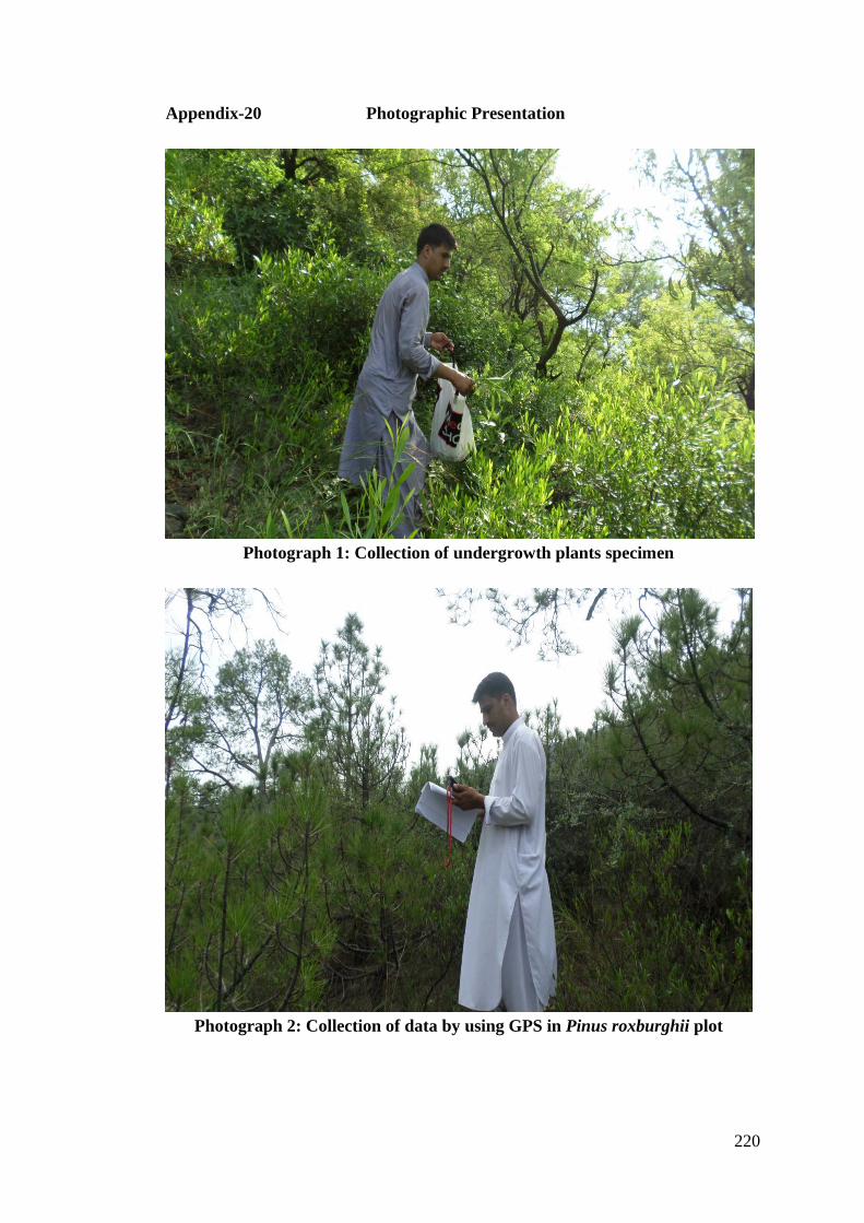
220
Appendix-20 Photographic Presentation
Photograph 1: Collection of undergrowth plants specimen
Photograph 2: Collection of data by using GPS in Pinus roxburghii plot

221
Photograph 3: Informal interview with local people during questionnaire survey
Photograph 4: Collecting informations from the local people through questionnaire
222
Photograph 5: Extraction of soil through supporters from the research plots
Photograph 6: Drying of soil sample in shade

223
Photograph 7: Woodlot plantations of Eucalyptus camaldulensis.
Photograph 8: Eucalyptus camaldulensis research plot

224
Photograph 9: Measurement of discharge rate of spring in the research area
Photograph 10: Acacia modesta research plot
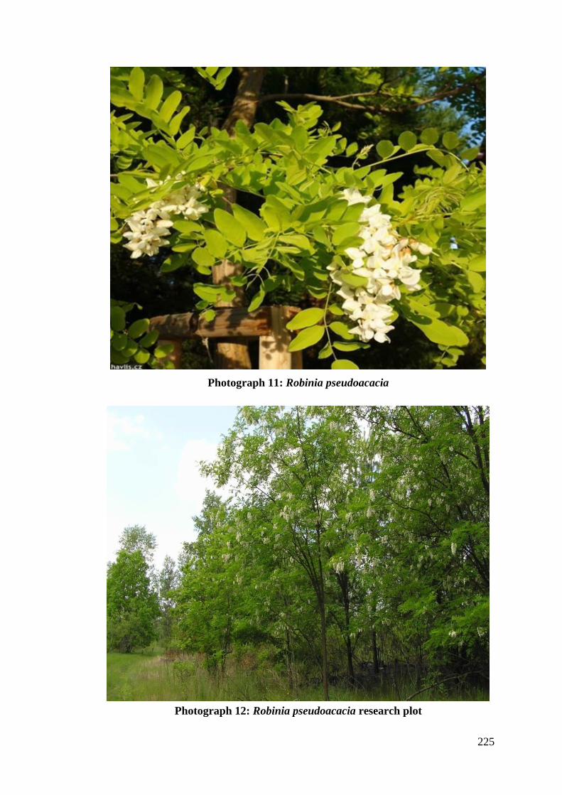
225
Photograph 11: Robinia pseudoacacia
Photograph 12: Robinia pseudoacacia research plot

226

227