phd thesis - atrium - university of guelph
TRANSCRIPT

Dissipation of Thermal Enrichment of Stormwater Management Ponds
by
Farshid Sabouri
A Thesis
presented to
The University of Guelph
In partial fulfillment of requirements
for the degree of
Doctor of Philosophy
in
Engineering
Guelph, Ontario, Canada
© Farshid Sabouri, December, 2013

ABSTRACT
DISSIPATION OF THERMAL ENRICHMENT OF STROMWATER MANAGEMENT
PONDS
Farshid Sabouri Advisor:
University of Guelph, 2013 Professor B. Gharabaghi
The intent of this research was to gain a better understanding of the effects of the design
parameters on the thermal impact of stormwater management wet ponds. The effect of
upland areas on inlet water temperatures of the ponds, thermal design modeling of the
ponds, and cooling trenches effects to mitigate stormwater ponds are investigated using
data collected from six stormwater ponds in the cities of Guelph and Kitchener, Ontario,
Canada.
The sensitivity analyses of the developed predictive artificial neural network (ANN)
model showed that the rainfall event mean temperatures significantly influenced
stormwater temperatures at the inlet of the ponds. The longest pipe length and pipe
network density are the two parameters that control the cooling effect of the underground
storm sewer system, as opposed to the impervious percentage of the catchment.
Concerning the key design parameters of stormwater ponds, larger permanent pool
volumes tend to release the warmer water resident in the ponds. Increasing travel path
ratio using baffles can lead to less mixing of the water that is resident in the pond with the
cooler fresh event runoff and therefore an increase in event mean temperature of outlet.

Increasing pond volume from 2000 to 4000 m³ - while keeping all other parameters
constant - results in an average increase of 5 °C in event mean temperature at the pond
outlet (EMTO); increasing travel path ratio from 0.6 to 1.2 leads to an average increase of
6 °C in EMTO.
Regarding the design parameters for stormwater ponds' cooling trench/ rock crib, the
results obtained from the sensitivity analyses of the ANN model revealed that the effect
of a cooling trench is significantly influenced by the initial temperature of the water and
rock in the cooling trench and influent temperature of the water. Reducing the hydraulic
depth from 0.8 to 0.3 m in the model shows a 2 °C improvement in the stormwater runoff
cooling efficiency of the trench. Increasing the length of the trench from 50 to 100 m in
the model confirms a 3 °C improvement in the stormwater runoff cooling efficiency of
the trench.

iv
Dedication
I would like to dedicate this Doctoral dissertation to my family. There is no doubt in my
mind that without continued kindness, support and encourage of my beloved and patient
wife and daughter, Bita, and Negar, I could not have completed this process, and I cannot
forget the sacrifices they made during last four years. I am greatly indebted to their
endless love and patience, which contributed significantly for the success of this research.

v
Acknowledgements
This research would not have been a success without the help and assistance from many
individuals. First, I would like to express my gratitude to my advisor Dr. Bahram
Gharabaghi for his continuous guidance throughout this research. I would like to give
special thanks to Professor Ed McBean for his support and all good markups and
feedbacks. I greatly appreciate the advisory committee members, Dr. Ed McBean, Dr.
Nicole Weber, Dr. Hermann Eberl for their support and time and very useful comments.
In addition, Dr. Ali Mahboubi put so much time, and I appreciate his help. I highly
appreciate Dr. Nandana Perrera for his help on fieldwork, data analysis and his insight
during the course of the study. Mr. John Palmer from GRCA was a great help for
technical review of cooling trenches. Insight from Dr. William Herb at the University of
Minnesota on his thermal model is also appreciated.
The research was possible due to the funding from the City of Guelph, the City of
Kitchener, GRCA, and AECOM. Mr. John Palmer and Gus Rungis form GRCA, Rachel
Burows and Don Kudo from the City of Guelph, Diana Lupsa and Grant Muphy from the
City of Kitchener, and Ray Tufgar from AECOM are particularly acknowledged for their
support and feedbacks. The design reports of stormwater management ponds were
provided by the cities of Guelph and Kitchener. The climatology data were obtained from
The Guelph Turfgrass Institute (GTI) and the Grand River Conservation Authority
(GRCA) monitoring stations in Guelph and Kitchener.

vi
Several people at University of Guelph including John Whiteside, Ken Graham, Bill
Trenuth, and Mani Seradj are also acknowledged for their help and support.
Undergraduates’ students Jacob Chol, Tamirat Tsigie, Mohammad Eftekhar, Richard
Chen, Mary Mikhail, Abbas Saeedy, and Patrik Cieslar were a great help in fieldwork
and organizing the data.

vii
Table of Contents
Dedication .......................................................................................................................... iv
Acknowledgements ............................................................................................................. v
Chapter 1 ............................................................................................................................. 1
Introduction ......................................................................................................................... 1 1.1 General Background ................................................................................................. 1 1.2 Research Needs ......................................................................................................... 5
1.3 Research Objectives .................................................................................................. 6
1.4 Thesis Organization .................................................................................................. 7
Chapter 2 ........................................................................................................................... 10
Literature review ............................................................................................................... 10 2.1 Ecological impacts of temperature increases .......................................................... 10 2.2 Stormwater ponds ................................................................................................... 11
2.3 SWM Ponds regulation ........................................................................................... 16 2.4 Temperature impact ................................................................................................ 19
2.4.1 Upland .............................................................................................................. 19 2.4.2 Pond ................................................................................................................. 20 2.4.3 Mitigation measures ......................................................................................... 22
2.5 General temperature modeling review .................................................................... 23
2.6 Artificial neural network modeling ......................................................................... 25
Chapter 3 ........................................................................................................................... 27
Evaluation of the Thermal Impact of Stormwater Management Ponds ............................ 27
3.1 Introduction ............................................................................................................. 28 3.2 Study description .................................................................................................... 28
3.2.1 Monitoring and data collection ........................................................................ 33 3.3 PCSWMM Modeling .............................................................................................. 34
3.4 Results and Discussions .......................................................................................... 35 3.4.1 Land Use Effect on Runoff Temperature ......................................................... 35 3.4.2 Thermal Enrichment in Ponds ......................................................................... 37
3.4.3 Bottom-Draw Outlet Effectiveness .................................................................. 37 3.4.4 Effectiveness of Cooling Trenches .................................................................. 39
3.5 Conclusions ............................................................................................................. 41 3.6 References ............................................................................................................... 42
3.7 Appendix to original paper ..................................................................................... 44 3.7.1 Location of sensors .......................................................................................... 44 3.7.2 PCSWMM model............................................................................................. 47

viii
Chapter 4 ........................................................................................................................... 49
Impervious surfaces and sewer pipe effects on stormwater runoff
temperature ....................................................................................................................... 49 4.1 Introduction ............................................................................................................. 51
4.2. Material and methods ............................................................................................. 53 4.2.1 Site selection .................................................................................................... 53 4.2.2 Planning Phase ................................................................................................. 54 4.2.3 Sensor installation and field procedures .......................................................... 55 4.2.4 Event mean temperature calculation ................................................................ 56
4.2.5 Overview of ANNs .......................................................................................... 58 4.2.6 Design of ANN ................................................................................................ 59 4.2.7 Feed-Forward Neural Networks ...................................................................... 59
4.3 Results and Discussion ........................................................................................... 61 4.3.1 ANN model development ................................................................................ 61 4.3.2 Calibration and Validation ............................................................................... 62
4.3.3 Sensitivity Analysis of the parameters ............................................................. 68 4.4 Conclusion .............................................................................................................. 71
4.8 References ............................................................................................................... 73
Chapter 5 ........................................................................................................................... 78
Thermal Design Modeling of Stormwater Management Wet Ponds ................................ 78
5.1. Introduction ............................................................................................................ 80 5.2 Material and methods .............................................................................................. 82
5.2.1 Site description................................................................................................. 82
5.2.1.1 Monitoring equipment and data collection ................................................... 83
5.3 Results and discussion ............................................................................................ 86 5.3.1 Thermal Enrichment in Ponds ......................................................................... 87
5.3.2 Ponds outlet temperature prediction using Artificial Neural Network (ANN) 90 5.3.3 Training and Evaluation of the ANN Model ................................................... 96 5.3.4 Sensitivity analysis of the parameters .............................................................. 98
5.4 Conclusion .............................................................................................................. 99 5.5 References ............................................................................................................. 101
Chapter 6 ......................................................................................................................... 108
Cooling effect of rock cribs on mitigating stormwater pond thermal
impacts ............................................................................................................................ 108
6.1 Introduction ........................................................................................................... 110
6.2 Material and methods ............................................................................................ 112 6.2.1 Cooling trenches ............................................................................................ 112 6.2.2 Overview of Artificial Neural Networks (ANN) ........................................... 114 6.2.3 Monitored cooling trenches and data collection ............................................ 115 6.2.4 Cooling trench models ................................................................................... 119 6.2.5 Unsteady (transient) state: .............................................................................. 119

ix
6.2.6 Development of an artificial neural network (ANN) model .......................... 122
6.3 Result and Discussion ........................................................................................... 125 6.3.1 Validation of the ANN model ........................................................................ 127 6.3.2 Sensitivity analysis of the variables of ANN model ...................................... 130
6.4 Conclusions ........................................................................................................... 135 6.5 References ............................................................................................................. 137
Chapter 7 ......................................................................................................................... 141
Conclusions and Recommendations for Future Research .............................................. 141 7.1 Research Summary ............................................................................................... 142
7.2 Conclusions ........................................................................................................... 145 7.3 Recommendations for Future Research ................................................................ 149
References ....................................................................................................................... 152
Appendix A- Detailed literature review .......................................................................... 164
Appendix B - Sample charts of collected data ................................................................ 168
Appendix C – Additional Tables .................................................................................... 174
Appendix D – Copyrights Release .................................................................................. 178

x
List of Tables
Table 3. 1 Ponds location .................................................................................................. 28
Table 3. 2 Ponds information ............................................................................................ 30
Table 3. 3 Pond 74 sensor locations and period of record ................................................ 33
Table 3. 4 Comparison of the inlet water temperatures .................................................... 36
Table 3. 5 Ponds 33 and 53 calculated events mean temperatures. .................................. 37
Table 3. 6 Pond 74 and church calculated event mean temperatures. .............................. 37
Table 3. 7 Pond 74 calculated EMTs for bottom draw and cooling trench ...................... 39
Table 4.1 Ponds related parameters .................................................................................. 55
Table 4.2 Collected data and calculated EMTs ................................................................ 57
Table 4.3 Input parameters for developed ANN models to predict EMTI ....................... 62
Table 4.4 Coefficient and different statistical measures for model evaluation and their
range of variability ............................................................................................................ 65
Table 4.5 Statistical performances of Train and Test value.............................................. 65
Table 4.6 Statistical performance of EMTI models .......................................................... 67
Table 4.1 Sensitivity analysis calculations ....................................................................... 69
Table 4.8 Relative importance of the variables ................................................................ 70
Table 5.1 Design parameters for the selected ponds ......................................................... 83
Table 5.2 Ponds 33 and 53 calculated events mean temperatures .................................... 88
Table 5.3 Pond 74 and Church calculated event mean temperatures ............................... 89
Table 5.4 Relative importance of the variables ................................................................ 92

xi
Table 5.5 Input parameters for developed ANN models to predict EMTO ...................... 94
Table 5.6 Statistical measures for model evaluation and their range of variability .......... 97
Table 5.7 Statistical performances of train and test value ................................................ 98
Table 6.1 Cooling trench key parameters ....................................................................... 115
Table 6.2 Collected data and calculated EMTs .............................................................. 118
Table 6.3 Heat transfer calculation for observed events ................................................. 124
Table 6.4 Input parameters to develop ANN models to predict “COOLING” ............... 126
Table 6.5 Coefficient and different statistical measures for model evaluation and their
range of variability .......................................................................................................... 129
Table 6.6 Statistical performances of “COOLING” model for Train and Test values ... 130
(CASE 1: 5 input parameters and Case 2: 2 input parameters as shown in Table 6.3) .. 130
Table 6.7 Sensitivity analysis results ............................................................................. 131
xii
List of Figures
Figure 1.1 Thesis flowchart ................................................................................................ 7
Figure 3. 1 Location of Guelph ponds .............................................................................. 29
Figure 3. 2 Location of Kitchener ponds .......................................................................... 29
Figure 3. 3 Pond 53 drainage area .................................................................................... 32
Figure 3.4 Pond 33 drainage area ..................................................................................... 32
Figure 3.5 Pond 81 drainage area ..................................................................................... 32
Figure 3.6 Pond 74 data 11 July 2011 rain event .............................................................. 34
Figure 3.7 PCSWMM result vs. observed values for pond 53 ......................................... 35
Figure 3.8 Water temperature at different depths of pond 74 .......................................... 36
Figure 3.9 location of sensors ........................................................................................... 45
Figure 3.10 Pond 33 collected data (summer 2011) ......................................................... 46
Figure 3.11 Pond 53 collected data (summer 2011) ......................................................... 46
Figure 4.1 Location of Guelph and Kitchener ponds . ...................................................... 53
Figure 4.2 Pond 33 watershed in Guelph .......................................................................... 55
Figure 4.3 An ANN with its inputs, hidden layers, bias and output ................................. 60
Figure 4.4 Artificial Neural Network Predictions of EMTI versus Observed EMTI ....... 67
Figure 4.5 The sensitivity analysis results of the ANN model for EMTI, IMP, LPL, and
PND................................................................................................................................... 71
Figure 5.1. Ponds 33 (left) and 53 (right) and location of sensors.................................... 85
Figure 5.2 Schematic of ponds 74 (left) and Church (right) and location of sensors ....... 86

xiii
Figure 5.3 PCSWMM model simulation for pond 53....................................................... 87
Figure 5.4 Pond water temperature profiles during dry weather ...................................... 90
Figure 5.5 The ANN Model consist of input layer ,hidden layers, and output layer ........ 93
Figure 5.6 Comparison of observed EMTO and predicted EMTO for two cases ............ 95
Figure 5.7 ANN model sensitivity analysis of EMTO to pond key design parameters ... 98
Figure 6.1 (a) Pond 33 and (b) Pond 53, 74 and Church cooling trenches ..................... 116
Figure 6.2 PCSWMM model for pond water level time series versus observed pond water
level during an event start (Pond 53) .............................................................................. 117
Figure 6.3 The ANN with its inputs, hidden layers, bias and output .............................. 125
Figure 6.4 ANN model predictions of COOLING versus Observed COOLING. .......... 127
Figure 6.5 The sensitivity analysis results of the ANN model ....................................... 132
Figure 6.6 A comparison between the Cooling calculated by ANN versus unsteady
model............................................................................................................................... 134
Figure 6.7 The difference between EMTO and CTinit Versus COOLING .................... 135
Figure 7.1 The flow of the thesis ................................................................................... 143

xiv
Notations Abbreviation Unit Definition
ANNs - Artificial Neural Networks
AspT °C Asphalt Temperature
BMPs - Best Management Practices
BOD Biological Oxygen Demand
COOLING °C Cooling Effect of a Cooling Trench
CRM - Coefficient of Residual Mass
CTinit °C Rock and Water Temperature in Cooling Trench Prior to Rainfall
d m Pond Depth
D hr Duration of Rainfall
DA ha Drainage Area
DO - Dissolved Oxygen
E - Coefficient of efficiency (Nash-Sutcliffe)
EMT °C Event Mean Temperature
EMTI °C Event Mean Temperature of Inlet
EMTR °C Event Mean Temperature of Rain
EMTO °C Event Mean Temperature of Pond's Outlet to Cooling Trench
GRCA - Grand River Conservation Authority
GTI - Guelph Turf grass Institute
HYD m Hydraulic Depth
ID - Index of Agreement
IMP - Impervious Percentage
L m Length of Trench
LPL m Longest pipe length
MA - Mean Absolute Error
MAE - Mean Absolute Error
Max - Max Absolute Error
MAPE - Mean Absolute Percentage Error
MI mm/hr Maximum Intensity of Rain
MLP - Multi-layer Perceptron
MINUHET - Minnesota Urban Heat Export Tool
MREST hr Minimum Residence Time
PF m³/s Peak Flow
PRB - Population Reference Bureau
PND m/ha Pipe network density
Q m3/s Runoff Flow Rate
R mm Rainfall
R2 - Coefficient of Determination

xv
SE - Root Mean Square Error
Sc - Sensitivity Coefficient
SCS - Soil Conservation Service
Sn - Normalized Sensitivity Coefficient
SMRE - Square of the Mean Root Error
SWM ponds - Stormwater Mangement Ponds
TES - Thermal Enrichment of Strom-water
TPR - Travel Path Ratio
TURM - Thermal Urban Runoff Model
Vct - Volume of the trench
Vrunoff - Volume of runoff
Vrunoff/Vct - Runoff Volume/Cooling Trench Volume
VOL m3 Pond Volume
WEP - Water and Energy Transfer Processes

1
Chapter 1
Introduction
1.1 General Background
Urbanization negatively affects stream hydrology since increasing imperviousness
changes the hydrologic balance in a watershed and, as a result, the frequency of flooding
and peak flow volumes, sediment loadings, and stream temperature increases in
urbanized areas (Booth, 2009). Stormwater runoff, long considered a nuisance in urban
areas, is now recognized as a threat to aquatic and riparian systems when dealt with
improperly. The main cause of the long term increase in average annual of stream
temperatures could be the result of the influence of humans on nature; the more
construction completed in a catchment the larger the increase in stream temperature
observed (Kinouchi et al. 2007). Cox and Bolte (2006) declare that thermal pollution
arises from human activities, changes to the landscape, and high temperatures flows
associated with stormwater runoff are causing changes in the temperature of a natural
body of water, such as a lake, rivers, or streams. Regression analysis by Kinouchi et al.
(2007) has shown that stream temperature in winter and early spring increased at the rate

2
of 0.11- 0.21 °C/year in segments that had a considerable increase in wastewater heat
input over the same period as a result of human activities.
During the summer months, stormwater runoff from impervious and paved surfaces can
reach temperatures above those seen in the natural environment. Thermally impacted
runoff may arise due to paved surfaces, which absorb and capture incoming solar
radiation and store this energy as heat. During a rainfall event, heat is transferred from
the pavement surface to stormwater runoff and then into creeks or ponds and, as a result,
temperature of creeks or ponds water rise.
Increasing the temperature of a creek or pond can disrupt the aquatic ecosystem and it
will be harmful for fish like trout (Herb et al., 2009). Fish like trout, as well as many
other aquatic organisms, have strict temperature requirements. In addition, trout and other
cold-blooded organisms lack the ability to control their own body temperature, leading
their behavior, metabolism, and other bodily functions to be regulated by the temperature
of the water around them. When water temperatures are elevated, trout populations may
diminish due to several factors such as, excessive metabolic rate, impaired juvenile
development, increased vulnerability to disease, altered migration patterns, and
competition with other fish (Jones, 2008). As an example, the brook trout is no longer
found in the lower reaches of the Hanlon Creek Watershed because of high summer water
temperature (MMM and LGL, 1993). Moreover, thermal shocks to receiving streams
from stormwater management ponds can be a source of chronic stress (Coutant, 1970).
Furthermore, there is no doubt that water temperature has direct and indirect effects on
nearly all aspects of stream ecology. For instance, the amount of oxygen that can be
dissolved in water is partly governed by temperature. As cold water can hold more

3
oxygen than warm water, certain species of aquatic invertebrates and fish with high
oxygen needs (including popular sport fish such as some trout and salmon) are found
only in cold waters. Metabolic rates of most stream organisms are controlled by
temperature (Dodds, 2002). Metabolic rate is the speed at which cells conduct the
chemical processes of life. As most aquatic animals are cold-blooded, their metabolic rate
is faster in warm water. Therefore, they need more food and oxygen in warm water and
release more wastes. Of course, this increase in metabolic rate occurs only up to a point
before the upper temperature tolerance is exceeded and the organism dies (Bulton, 2008).
Thermal pollution from urban runoff is a significant contributor to the degradation of
cold-water ecosystems (Boulton, 2008; Herb et al., 2008; and Jones, 2008). In addition,
water temperature is one of the most important factors influencing the distribution of
aquatic organisms (Cairns et al., 1971; Poole et al., 2009).
Temperature also influences the rate of photosynthesis by algae and aquatic plants. As
water temperature rises, the rate of photosynthesis increases provided there are adequate
amounts of nutrients (Dodds, 2002).
Thermal enrichment due to urbanization arises from three sources: 1- surface area of
open water, such as ponds and streams 2- Artificial impervious surfaces in urban areas 3-
Industrial discharges. Water temperature is an important water quality index in an aquatic
environment since it influences at least three principal facts, which are 1- the aquatic
ecosystem 2- biological and chemical reactions and 3- physical properties of water, such
as density. Compared with industrial thermal discharges, thermal enrichment of receiving
water bodies due to urban stormwater as a source of thermal pollution has been

4
neglected; however, thermal enrichment is being recognized as a potential threat to the
aquatic environment (Li and James, 2004).
The other causes of increased stream temperature fluctuations could be loss of riparian
vegetation, changes in channel morphology, and/or reduction in groundwater flow to
streams (Arrington, 2009). However, the extent of impervious surfaces in urban areas is a
major source of thermal pollution in cold climates and threatens the health of cold-water
ecosystems (Thompson et al., 2008).
Some popular management practices to limit elevated runoff temperatures are shading,
using lighter reflective colors for paving and construction material, promotion of
infiltration using permeable pavement, and use of stormwater pipe materials with a
higher convective heat transfer coefficient to dissipate heat into the ground and cooling
trenches (Arrington, 2009; Coutant, 1970).
Stormwater management ponds are the popular option for mitigating the flooding effects
of stormwater runoff on streams (Scheueler and Galli, 1995). In addition, it is widely
accepted that stormwater management ponds (SWM ponds) can be effective at removing
or reducing the concentration of total suspended solids (TSS) and associated
contaminants from urban and industrial surface runoff during storm events (Anderson,
2002). However, ponds have the potential of negative thermal effects on aquatic habitat;
one aspect of negative thermal effects could be the disruption of the aquatic ecosystem
due to thermal shocks to receiving streams (Poole et al. 2009). Conservation authorities
and other related stormwater management parties have been proactively trying to find
solutions to address the thermal effects of SWM ponds; but lack of sufficient data and
information hinder obtaining satisfactory results. The purpose of this research includes:

5
(1) the study of thermal changes to traditional stormwater management ponds from
upland areas; (2) assessment of and formulation of upland area effects on inlet water
temperature of stormwater management ponds; (3) thermal design modeling of
stormwater management wet pond; and (4) rock cribs’ cooling effect on stormwater
management pond thermal mitigation.
1.2 Research Needs
Very few studies and data are available for Ontario on the thermal effects of stormwater
management ponds and temperature monitoring of existing ponds as well as performance
of mitigation techniques such as cooling trenches. The research has been developed in
response to recognition of the lack of sufficient information and data in Ontario with
respect to potential adverse thermal enrichment of stormwater management ponds on
sensitive aquatic habitats.
Considerable attention has been given to thermal enrichment of stormwater runoff by
paved surfaces using computer models. Over the last several years, Artificial Neural
Network (ANN) modeling has been used in a variety of complex hydrological and
hydraulic processes. However, there is a lack of information regarding the use of an
artificial neural network in modeling urban runoff temperature and stormwater
management ponds. This study was an attempt to fill the knowledge gap that currently
exists in determining:
i) The impact of urbanization on stormwater management ponds’ inlet water
temperature during a rainfall event using artificial neural networks,

6
ii) Thermal impact of stormwater management ponds with respect to design
parameters, and
iii) Cooling trench effectiveness as part of stormwater management ponds outlet
structure to reduce the water temperature from pond to receiving systems.
Furthermore, the intent of this research was to achieve a better understanding of the
effects of stormwater management ponds on the summer thermal regime. Six stormwater
management ponds were investigated by analyzing monitoring data collected in Guelph
and Kitchener. Based on the monitoring of the sensitive locations (such as inlet and
outlet ) of the monitored ponds, the intent was to identify and quantify the sources and
heat transfer in urban watersheds and to develop predictive models for water temperature
for different parts of the system such as ponds’ inlet, ponds' outlet and cooling
trench/rock crib. The need for design capability for cooling trenches to mitigate
potential adverse effects of SWM ponds and, the effectiveness of those cooling trenches
if constructed, are the other motivators to develop this study since very few studies and
data are available on temperature monitoring of existing cooling trenches and their
effectiveness is of interest.
1.3 Research Objectives
The main objectives of the study are to: (1) quantify the effect of upland/drainage area
landuse on stormwater runoff temperature; (2) evaluate the effect of key stormwater pond
designs on runoff temperature; and (3) examine the effectiveness of cooling trenches in
mitigation of runoff temperature.

7
1.4 Thesis Organization
This thesis follows a manuscript format with published and un-published papers. Chapter
three to six contain separate papers, each discussing different aspects of the research. All
the papers include an introduction and separate sections on the methodology, results and
discussion, and conclusion. Although the concept of thermal effects is common between
the chapters, each chapter is independent of the others.
This dissertation is organized into seven chapters as shown in Figure 1.1.
Figure 1.1 Thesis flowchart
The background, research needs, and objectives are discussed in Chapter 1.
A literature review on stormwater ponds is provided in Chapter 2.

8
Chapter 3 discusses the thermal impacts of stormwater management ponds. This chapter
presents temperature-monitoring data from six monitored stormwater ponds; three were
located in the City of Guelph and three in the City of Kitchener. The chapter primarily
focuses on the investigation and evaluation of the thermal effects of traditional
stormwater management ponds (SWM ponds). The evaluation includes examination of
the effects of upland area on thermal enrichment and effectiveness of current thermal
mitigation methods. The preliminary results of the monitoring program are presented in
this chapter. In addition, it is a published paper in CHI monograph 2012.
Chapter 4 extends the results of Chapter 3, to assess and formulate the upland area effects
on inlet water temperature of stormwater management wet ponds, and provides a
predictive artificial neural network to predict the inlet water temperature of the ponds.
This chapter has been published in the Journal of Hydrology
Chapter 5 proposes a thermal design model of stormwater wet ponds. Upland area effects
on inlet water temperatures of stormwater management pond and a predictive artificial
neural network have been presented in previous chapter. The current chapter investigates
thermal enhancement within the studied ponds. An ANN model was trained which
provides a good level of accuracy to predict the event mean temperatures at the pond
outlet. The model then was used to find the sensitivity of model variables on the event
mean temperatures of the pond outlet. This chapter was submitted to Journal of
Hydrology on May 2013.
In Chapter 6, the cooling effect of cooling trenches/rock cribs for thermal mitigation of
stormwater pond is discussed. Flow from ponds' outlet (discussed in Chapter 5) goes to
the cooling trench and then to the receiving system. Therefore, there is a need to evaluate
9
the performance of the cooling trench in order to consider warming and cooling effects in
different part of the system from upland to receiving water body. Thus, monitoring
results along with developed artificial neural network model are employed to advance the
knowledge of key design parameters influencing performance of the rock crib or cooling
trench.
Chapter 7 concludes this study and gives recommendations on thermal effects from
upland area up to the receiving systems.
Detailed literature review of some heat transfer (between runoff and paved surfaces)
models, sample charts of collected data and additional tables are presented in appendices.

10
Chapter 2
Literature review
2.1 Ecological impacts of temperature increases
Brett (1952), Coutant (1970), and Fry (1967) are some of the Canadian researchers who
began studying the effects of water temperature on salmon species. The unfavorable
effects of quick changes in water temperature on fish and other freshwater biota have
long been recognized (Agersborg, 1930). Multiple anthropogenic stressors have affected
streams over the past decades. Some of these stressors include increased watershed
imperviousness, destruction of riparian vegetation and change in climate. Water
temperature, ecological processes, and stream biota change due to these stressors (Nelson
and Palmer, 2007). It is recognized that aquatic biota slowly adapt to elevated water
temperatures and can tolerate a higher maximum temperature up to certain point.
However, rainfall events may cause hourly increases in the temperature of water being
discharged from stormwater ponds by up to 6.6 °C in an urban area (Lieb and Carline,
2000).
Freshwater fish and most other aquatic biota are poikilotherms and have little or no heat
production or insulation from the environment meaning their body temperatures are
regulated by their surroundings. Thus, their metabolism and physiological processes are

11
directly related to their surrounding water temperature. Rapid changes in water
temperature have detrimental effects to fish and other freshwater biota (Agersborg,
1930). Fish, especially trout and salmon, possess some of the most inflexible temperature
requirements. Most trout and salmon prefer water temperatures between 4 to 21 °C, with
increased temperatures leading to injury or death (Jones and Hunt, 2007). The main
ecological effects and changes to fish and aquatic biota due to higher water temperature,
as have been reviewed by other researchers, are:
(1) Rates of egg hatching and changes in growth rates,
(2) Diversity and change in community structure,
(3) Dissolved oxygen depletion,
(4) Organic matter decomposition rates,
(5) Increases in diseases,
(6) Composition of primary producers,
(7) Digestion rate and food requirement,
(8) Swimming behavior,
(9) Avoidance of predation or capturing of prey, and;
(10) Mortality (Marsalek et al., 2002).
2.2 Stormwater ponds
Discharges of urban stormwater may cause numerous adverse effects on receiving waters,
including flooding, erosion, sedimentation, temperature rise, dissolved oxygen depletion,
reduced biodiversity, and the associated impacts on beneficial water uses (Marsalek et al.,
2002). Over the past decade, stormwater ponds have been identified as an effective
structural best management practices (BMPs) for stormwater quantity and quality control

12
by numerous authors, and have been widely applied across Ontario, Canada, the United
States, Australia and some European countries (Anderson, 2002).
Dry and wet ponds are end-of- pipe facilities, which are usually required for flood and
erosion control. Although lot-level and conveyance controls can reduce the size of the
required end-of-pipe facilities, stormwater ponds remain a practical option for mitigating
the impact of uncontrolled stormwater runoff on streams (MOE Manual, 2003). Both dry
and wet ponds are detention basins designed to store collected stormwater runoff and
release it at a controlled rate. A wet pond maintains a permanent pool of water between
storm events, which is the main difference between wet and dry ponds. The most
common end-of-pipe stormwater facilities used in Ontario are wet ponds. Inlet
mechanisms of the wet pond allow stormwater supplied by stormwater pipes and
conveyance system to go into the pond. A small basin (a sediment forebay) is located
before the main pool. The water, which flows into the forebay, slows down and drops
most of its sediment load prior to entering the permanent pool. This mechanism prevents
erosion and re-suspension of the settled sediment in the main pool. Stormwater flows into
a wet pond are diluted by the main pool, and usually there is sufficient time between
events for sediment trapped in the permanent pool to settle. Wet ponds have an active
storage volume. The active storage volume is needed to store the runoff from large
storms which otherwise contributes to erosion and flooding of the receiving stream.
Sediment removal and flooding concerns are resolved by an outlet structure, which
allows the pond to detain water long enough for sediment to settle, and reduce flow rates
significantly (MOE guidelines, 2003).

13
The stormwater management planning and design manual from MOE (2003) provides
design guidelines for SWM ponds. For instance, topography, soil type, depth to bedrock,
depth to seasonally high water table, and drainage area need to be considered in order to
evaluate SWM ponds. Some other guidelines are listed as: (1) locate the SWM ponds
outside of the floodplain, (2) assess the effects on corridor requirements, (3) functional
valley land values, and the fluvial processes in the floodplain, and (4) the outlet invert
elevation and the overflow elevation must be above the 2 and 25 year flood lines
respectively. Also, the Center for Watershed Protection (CWP, 1997) provides a number
of recommendations with respect to design modifications for cold climate, such as: (1)
increased storage volume to resolve volume reduction owing to ice, (2) sizing and
location of inlets and outlets to prevent ice clogging, (3) prevention of early spring
drawdown to avoid discharge of water with low oxygen or high chloride levels. In regard
to modification of inlet and outlet design, the CWP design supplement recommendations
are listed as follows: (1) inlet and outlet pipes' slopes to be greater than 1%, (2) minimum
pipe diameters of 450 mm, (3) no partially submerged or submerged inlets are
recommended, and (4) submerged outlet to be 150 mm below the expected maximum ice
depth.
Anderson et al. (2002) investigated an on-line pond in Ontario, which was constructed in
1982. They report three main concerns within the categories of initial design, which are
operation and maintenance, performance, and adaptive design. Initial design may include
the use of on-line versus off-line ponds, which could be effective in observing pond
performance, accessibility for maintenance, retrofit activities, pond physical dimensions,
landscaping, and the public’s perception. Some other concerns related to performance of

14
the pond are listed as; seasonal effects, uncertainty in performance introduced by
uncontrollable perturbations in the environment, and changes in performance due to new
issues such as habitat creation (Anderson et al., 2002).
In a research study conducted by Persson (2000) with regard to design aspects of
stormwater management ponds, it has been found that length-to-width ratio, location of
inlets and outlets, subsurface berm, and an island in front of the inlet, have large
influence on the hydraulic performance of a pond. The other important factors are named
as vegetation, hydrologic regime, and organic loading. Hydraulic aspects of ponds can be
defined as hydraulic efficiency and hydraulic performance. Hydraulic efficiency is
described as how well the incoming water is distributed within the pond; low amounts of
mixing and dead zone are two characteristics that reduce the hydraulic efficiency of
ponds. Hydraulic performance is a wide concept that covers more aspects of the flow
conditions, and it is less value-oriented; for instance, short-circuiting and lag time are
measures of performance. Hydraulic performance is mainly related to shape including
baffles, topography, vegetation, flow, location of inlets and outlets, wind, and
temperature (Persson, 2000). The hydraulic conditions can be analyzed through the
concepts of effective volume ratio and dispersion (the degree of mixing). In ponds, the
effective volume ratio is primarily determined by the length-to-width ratio, while
dispersion determined by the length-to-width ratio, and depth and flow velocity, to lesser
degrees (Persson and Wittgren, 2003).
To summarize, hydraulic design of ponds is the key control of the performance and
efficiency of ponds. All mitigation techniques concerning thermal enrichment of the
ponds (provided in guidelines, e.g., MOE, 2003) are implicated within hydraulic design.
15
As a result, if ponds are designed and located with no regard for the immediate
environment, they can have negative impacts in sensitive stream systems (Schueler and
Galli, 1994). The positive and negative impacts of ponds on local, upstream, and
downstream conditions have been investigated by Schueler and Galli. They investigated a
series of seven pond configurations and different pond designs, and they reviewed
environmental impacts associated with stormwater ponds. In more explicit term, channel
protection, pollutant removal and flood attenuation, wetland creation, waterfowl habitat,
retention of open space and warm water fishery are listed as positive impacts of ponds on
downstream ecosystems. Some negative impacts named were forest habitat loss, fish
barrier, stream warming, dry weather water quality, and interruption of drift and bed load.
Moreover, Schueler and Galli claim, “once a critical threshold of watershed development
has been exceeded, watershed Delta-T overwhelms any effort to reduce thermal
enrichment, where Delta-T is the change in urban summer stream temperatures from an
undeveloped reference stream baseline, and it is a direct function of watershed
imperviousness. The magnitude of a wet pond Delta-T appears to be a direct function of
the size of the permanent pool in relation to the contributing watershed. Masalek et al.
(2002) assessed the effectiveness of SWM ponds concerning pollution control, such as
heavy metals and polycyclic aromatic hydrocarbons, as well as sediment control. The
authors claim that the pond was affected by the cumulative impacts associated with
polluted sediments rather than by acute impacts of stormwater. In addition, the pond
accumulates sediments and toxicants. The main observation was that taxa richness and
total counts of benthic organisms did not vary much when moving from upstream to
downstream of the pond (Marsalek, 2002).

16
2.3 SWM Ponds regulation
SWM ponds must meet the requirement assigned by regulators; at the federal, provincial
and municipal level including Conservation Authorities' regulations and policies. Design
specification and requirements manuals and legislations are the main existing sources to
follow by third parties in regard to stormwater management (SWM) ponds. Regulations
which affect on SWM ponds and their thermal impacts can be found in the Fisheries Act
(Fisheries and Oceans Canada/DFO, 2003), Clean Water Act (Ministry of Environment/
MOE, 2006), Ontario Water Resources Act (MOE, 1990), and The Endangered Species
Act (Ministry of Natural Resources/MNR, 2007). The provincial Clean Water Act (MOE,
2006) has no specified condition aimed at stormwater ponds, however, if they are
considered a potential transport pathway, they may require reassessment of the hazard
conditions associated with a wellhead protection area (WHPA) (CVC thermal study
report, 2012). A wellhead protection area is the area around a well where land use
activities have the potential to affect the quality and quantity of water that flows into the
well. Since stormwater ponds can interact with both ground water and surface water, they
may be a threat to increase groundwater or surface vulnerability in WHPA analysis.
In general, SWM ponds purposes are: 1- To implement a stormwater management
system with respect to the ecosystem and watershed, as dynamic and living systems
which needs to incorporate with the urbanized human community, in order to manage
flooding and quality of the stormwater flows, 2- To ensure fulfillment with the entire
applicable municipal requirements and provincial legislation, and; 3- To advance the
development of safety-oriented and naturalized SWM ponds that extant a visually

17
pleasing feature to the community (Design specification and requirements manual
London, Ontario, 2010).
In the US Environmental Protection Agency (US EPA) handbook (2003), temperature is
indicated in a list of top ten impairments in the United States. However, the percentage of
published stormwater management related reports that refer to temperature is just 4.5% of
total published reports. (US EPA Handbook, 2003). Water temperature is an important
factor in terms of habitat and oxygen depletion because water temperature has a direct
effect on aquatic habitat (especially cold-water habitat) and soluble oxygen. Oxygen
depletion and habitant alternation are in list of top ten of impairment according to US
EPA Handbook (2003).
Most methods to address water quality objectives are more concerned with pollutant
removal than water temperature.
As mentioned, the construction and operation of SWM ponds must conform to a number
of provincial regulations administrated by the local Conservation Authorities (CAs),
Ministry of Natural Resources (MNR), and Ministry of Environment (MOE). The
Conservation Act allows Conservation Authorities to make local regulations that are
directly related to stormwater ponds. Grand River Conservation Authority (GRCA) has a
watershed management plan that identifies cold-water streams which has been updated as
of February 2013. Also, recognition of thermal enrichment of stormwater management
ponds by GRCA is one of the key motivators to much of the current research and studies
situated in the GRCA jurisdiction (Guelph and Kitchener). In 2002, the credit Valley
Conservation (CVC) also developed a Fisheries Management Plan, in which the thermal
impact of SWMP on the discharge water is identified.

18
The Ontario Ministry of the Environment (MOE) design guidelines generally describe
strategies aimed at reducing the level of total dissolved solids (TSS) and associated
pollutant loads to receiving streams. In 1991, MOE released a report entitled “Stormwater
Quality and Best Management Practices”, which outline, structural and non-structural
Stormwater Management Practices (MOE, 1991). The main purpose of the report was to
develop and implement best management practices in urban development and
redevelopment plans. In 1994 another manual entitled “Stormwater Management
Practices Planning and Design Manual” was published which was focused on techniques
to improve water quality discharged from stormwater ponds. The most recent version of
the guidelines (MOE, 2003) was extended to incorporate erosion considerations and
water balance. Section 3.3.4 of the MOE manual (2003) identifies temperature as a major
concern to fish habitat, especially where the receiving surface waters are cold-water
streams. The manual refers to a number of reports, which show that facilities such as
stormwater ponds increase the temperature of water before discharging to the receiving
stream mainly due to absorbing solar energy. There are some design considerations
required to remove TSS from surface runoff in SWM ponds, such as increased water
storage and retention time, which can also result in warming of the stored surface water.
In turn, the discharge of warmer water may have a detrimental effect on the aquatic
habitat in the nearby receiving stream. Sensitivity of the receiving waters to thermal
impacts must be addressed when considering or designing stormwater management
ponds.

19
The use and construction of SWM ponds is increasing in the rapidly developing areas of
southwestern Ontario. Several municipalities have hundreds of SWM ponds within a
single watershed. Therefore, the potential for individual, combined, and cumulative
impacts within a watershed is significant.
Since SWM ponds can act as both a sink and a source for pollutants, they may be best
considered as transport pathways. Without proper design and maintenance, the
concentration of substances in the discharge from these ponds may exceed provincial
water quality guidelines. In addition, elevated water temperatures may be considered a
"Deleterious Substance" or a HADD (Harmful Alteration Disruption or Destruction)
under the federal Fisheries Act (CVC Thermal study report, 2011). Furthermore,
according to MOE guidelines (2003), Low Impact Development (LID) is a type of
stormwater management practice, which can be applied in small-scale hydrologic
controls (subdivision scale) to more closely mimic pre-development hydrology. The idea
is to minimize the impervious surfaces and have the same amount of runoff in post
development condition. Since runoff temperature can increase as a result of increased
impervious areas. Impervious surfaces absorb solar radiation and transfer stored heat to
runoff (US EPA Guideline, 2009).
2.4 Temperature impact
2.4.1 Upland
The thermal regime of urban streams tends to be warmer than for undisturbed systems
(Pluttowski, 1970; Schueler and Galli, 1994). The cumulative impact of land cover
changes as a result of development has some major consequences, which are:

20
(1) Increased volume of runoff as a result of less infiltration and evapotranspiration,
(2) Increased peak flow of runoff as a result of increased consequence efficiency with
impervious surfaces,
(3) Increased duration of discharge as a result of greater flow rates and volumes which
can undermine the stability of the stream channel, also bank cutting, and erosion may
occur,
(4) Increased pollutant loadings – pollutant can transport from impervious areas to
receiving systems since impervious areas are a collection site for pollutants, and;
(5) Increased temperature of runoff as mentioned impervious surfaces absorb solar
radiation transfer heat to stormwater runoff during a rainfall event. High runoff
temperatures may have harmful effect on receiving systems (US EPA Guideline, 2009).
Urbanization can adversely affect stream hydrology as impervious surfaces may increase
the frequency of flood and peak flow rates, sediment loads and stream temperature
(Booth and Bledsoe 2009; Kieser 2004; Nelson and Palmer 2007; LeBlanc 1997; Brown
and Fitzgibbon 1996). Thermal pollution from urban runoff is a significant contributor to
the degradation of cold-water ecosystems (Boulton 2008; Herb et al. 2008). Galli (1990)
reported that the increase in summer stream temperatures in an urban watershed was
related to the degree of imperviousness of the contributing area by a factor of 0.09 °C for
every 1% increase in impervious area.
2.4.2 Pond
In a joint study conducted by Ham et al. (2006) at Temple University and the
Philadelphia Water Department using data from temperature loggers installed in ponds; it
was found that water temperature at outlet of the pond was up to 4 °C warmer than the
21
Pennypack Creek from which inlet water is received, at the beginning of the summer. The
water temperature was 6 °C higher by the end of summer for the studied pond (Ham et
al., 2006). In addition, Herb et al. (2009) in their study regarding simulation of
temperature mitigation by a stormwater management pond claim that on average, pond
outflow temperature was 1.2 °C higher than inflow temperature (Herb et al., 2009). In
addition, graphs presented in Appendix- B from the collected temperature data during
course of the current study confirm that pond outlet’s water temperatures were higher
than inlet water temperatures.
Under the assumption of completely mixed condition, the average of temperature of the
pond is a function of thermal energy stored in the pond, the specific heat, and pond
volume. However, in the case that stormwater management pond does not operate under
completely mixed conditions, the temperature measurement at one location may not
represent the average temperature of the pond. Determination of the temperature variation
within the pond would be of interest due to significant temperature differences in the
pond. Furthermore, recorded data from Kingston pond in Ontario showed surface water
was 3.6 °C warmer than the average temperature recorded at the bottom of the pond with
average depth of one meter (Burn et al., 2000).
Solar radiation, air temperature, and ground temperature are the four basic contributors to
direct heating of stormwater ponds. The surface area of a pond is one aspect, which has
influence on the degree to which pond water warms. The shape and orientation of the
pond, bottom draw outlet, shading (vegetated floating islands or artificial shade systems),
and nighttime release have influence on the outlet water temperature of a pond (CVC
Thermal study report, 2011).

22
2.4.3 Mitigation measures
If ponds are designed and located with no regard for the immediate environment, they
can have negative impacts in sensitive stream systems (Schueler and Galli, 1994). The
2003 MOE manual includes a brief section of mitigation procedures to deal with water
temperature increases in stormwater ponds. Techniques, which were identified to mitigate
thermal effect of ponds, as mentioned, are riparian planting, bottom-draw outlet,
subsurface trench outlet, nighttime release, outlet channel design, use of shading and
construct cooling/infiltration or rock cribs. Furthermore, there are some design practices,
which can be employed to reduce the magnitude of a pond’s thermal enrichment such as:
(1) Shading the channel and outfall,
(2) Minimum use of concrete in the low flow path,
(3) Reducing the volume of permanent pools,
(4) A north –south direction pools alignment (when pond has proper shading since
provided shading would be more efficient due to angle of the sun), and;
(5) Deep water releases (Schueler and Galli, 1994).
To mitigate thermal impacts of stormwater management ponds, CVC suggested
researching, designing and promoting the use of cooling trenches, bottom-draw outlets
and other similar techniques.
Concerning cooling trenches, the effectiveness of cooling trenches is one of the important
issues in design and performance of stormwater management ponds. Research conducted
at University of Wisconsin (Thompson et al. 2008) revealed that:
(1) Higher flow rate decreased the time for effluent water temperature to reach the
influent water temperature.

23
(2) Higher influent water temperature decreased the time for a specific temperature to be
realized in the rock crib/cooling trench.
(3) Size of the crib had an influence to decrease influent temperature, and the larger cribs
were more effective at reducing water temperature for constant flow rate and influent
temperature.
(4) Cribs that were initially full of water prior to events pronounced more cooling effects
as opposed to when cribs were initially empty.
(5) The ability of rock cribs to reduce runoff temperature is confirmed and rock cribs
could be used as a practicable management practice when applicable.
However, there is a need to optimize the cooling trench design related to pond outflow, as
to reduce cost and increase efficiency. For instance, questions such as;
- Which size of crib would be the best according the pond effluent, and;
- Which size would be the best fit to cool down the water coming from the pond
into the cooling trench during large events, must be considered.
2.5 General temperature modeling review
Considerable attention has been given to thermal enrichment of stormwater runoff by
paved surfaces using computer models (Galli 1990; Xie and James 1993; James and
Verspagen 1996; Picksley and Deletic 1999; Van Buren et al. 2000; Ul Haq and James
2002; Jia et al. 2002; Roa-Espinosa et al. 2003; Herb et al. 2006; Thompson, et al. 2008;
Janke et al. 2008). James and Verspagen (1997) developed the “decade method” to
estimate the temperature of surface runoff from paved surfaces. They reported mean
runoff temperature as a linear function of initial pavement temperature before wetting.
Picksley and Deletic (1999) performed a statistical analysis using graphical observations

24
of thermal trends, analysis of the event mean temperature (EMT), and analysis of thermal
exponential decay theory. The WEP model (water and energy transfer processes model)
developed by Jia et al. (2002) predicts changes in water and energy budgets associated
with land use changes in urbanized and partially- urbanized watersheds. The TES model
(Thermal Enrichment of Stormwater) developed by Haq and James (2002) is a direct
application of James and Verspagen’s work. The TES model is characterized for a big
difference made in the calculation of the Reynolds Number. Herb et al. (2006) developed
the MINnesota Urban Heat Export Tool (MINUHET), which is an analytical model
capable of simulating the flow of stormwater surface runoff and its associated heat
content for small watersheds. The TURM model developed by Roa-Espinosa et al. (2003)
and advanced by Thompson et al. (2008) is a useful tool for determining runoff
temperature for typical urban areas, although the model is event based, its major
limitation is the rainfall events are treated with uniform intensity as a consequence of
using the SCS curve number method for prediction of runoff hydrographs.
Several models were reviewed with respect to ponds’ water temperature. The most
important three models are listed here. The first model is a numerical simulation of the
hydraulic and heat transfer in ponds, which was proposed by Herb et al. (2006). The
mentioned model is used for developing MINUHET. The second model is PHATR,
which is introduced by Lamoureux et al. (2006). PHATR is a mathematical model based
on heat energy balance to predict pond temperatures. Moreover, the third model, MAPT,
uses a heat balance to estimate average monthly pond temperature; this model was
developed by Klemeston and Rogers (1985).

25
Cooling trench-reviewed models are the Thermal mixing model by Thompson et al.
(2008), Rock crib model as part of MINUHET model and Steady-state heat transfer
approach. Appendix A provides a literature review on thermal models and appendix C
presents a summary of the models as tables.
2.6 Artificial neural network modeling
Artificial neural networks (ANNs) are data processing tools that simulate the structure
and function of the human brain. A neural network integrates an interconnected data
processing method. The neural network can learn data with a learning algorithm using a
set of data. In general, neural networks are trained to perform a task by learning from a
set of training instances. Parallel-interconnected data processing can lead to much greater
computational power. This enables ANNs to model complex data even if data are
imprecise and noisy. Training an ANN is crucial to achieving the proper network
topology and training algorithm. Feed-forward neural networks have been the
most commonly used models. The feed-forward processing involves an input layer in
which each input value is multiplied by a corresponding weight. These weighted values
are then passed into the hidden layer where the model sums the weighted inputs and bias.
Finally, the model passes the sum of all previously weighted inputs and bias by a transfer
function to provide the result to the output layer.
Over the last several years, ANN modeling has been used in a variety of hydrological and
hydraulic phenomena (Chua et al. 2011; He et al. 2011; Dolling and Varas 2002;
Cigizoglu 2003; Riad et al. 2004; Hu et al. 2005; Sarangi and Bhattacharya 2005; Tayfur
et al. 2005; Giustolisi and Simeone 2006).. ANNs have shown a great ability in modeling

26
complex environmental systems with both linear and nonlinear relations. The current
study provides the application of ANN modeling on thermal enrichment of runoff and
stormwater management ponds. In addition, the ANN models provided in chapters 4 to 6
were developed for the first time with the purpose of thermal assessment using Tiberius
software.

27
Chapter 3
Evaluation of the Thermal Impact of Stormwater Management
Ponds
This chapter investigates the thermal effects of traditional stormwater management ponds
(SWM ponds) to evaluate the thermal impact of these SWM ponds. The evaluation
includes examining the effects of upland area characteristics on thermal enrichment and
effectiveness of current thermal mitigation methods, such as bottom draw outlets and
constructed cooling trenches.
This chapter is directly from the following published conference paper:
Sabouri, F., Gharabaghi, B., Perera, N.,McBean, E. (2012). “Evaluation of the Thermal
Impact of Stormwater Management Ponds.” CHI- Monograph 2012.

28
3.1 Introduction
Urbanization causes temperature increases in stormwater runoff. Asphalt and other
impervious surfaces absorb the heat energy and during the rainfall events, the stored heat
is transferred to the runoff, which eventually discharges to a water body (Thompson et
al., 2008). Water temperature is a critical environmental factor for cold-water fisheries
because most aquatic organisms have a specific temperature range that they can tolerate
(Booth and Bledsoe, 2009). Thermal pollution can also affect ecological functions of
aquatic species such as spawning and growth (Selong et al., 2001; Armour, 1991).
Stormwater management ponds remain a popular option to control runoff, total
suspended solids (TSS) and pollution, among other practices. However, SWM ponds can
have a thermal impact. This study has been developed in response to recognition of the
lack of sufficient information and data in Ontario with respect to potential adverse
thermal enrichment of SWM ponds on sensitive aquatic habitats.
3.2 Study description
In this study, six SWM ponds have been monitored during three summers (2009 to 2011).
The locations of the ponds is given in Table 3.1, and shown in Figures 3.1 and 3.2.
Table 3. 1 Ponds location
Pond City Location or Major intersection
53 Guelph York Road and Watson Road
33 Guelph Edinburgh Rd S and Southcreek Trail, next to Preservation Park
81 Guelph Edinburgh Rd S and Gordon St, East of Carrington Dr
74 Kitchener The northwest corner of Bleams Road and Fischer–Hallman Road
83 Kitchener Robert Ferrie SWM (Topper Swamp–West pond), Robert Ferrie Dr
Church Kitchener 1880 Strasburg Rd (private facility)

29
Figure 3. 1 Location of Guelph ponds
Figure 3. 2 Location of Kitchener ponds

30
The Guelph ponds have catchment areas of 79 ha, 19.4 ha and 5 ha for pond 53, pond 33
and pond 81 respectively. The Kitchener ponds are pond 74, pond 83, and Church with
drainage areas of 35.8 ha, 10.8 ha, and 5.1 ha respectively. Surface areas and volumes of
the ponds are given in Table 3.2. The receiving system for ponds 33 and 81 in Guelph is
the Hanlon Creek and for pond 53 is Clythe Creek. Water from pond 74 in Kitchener
discharges to the wetland next to it and the receiving systems for pond 83 and Church are
Doon South Creek and Strasburg Creek respectively. Furthermore, ponds 53, 81, 74 and
Church have constructed cooling trenches, which are monitored during the course of the
study.
Table 3. 2 Ponds information
Pond Catchment area (ha)
Volume (m³)
Surface area (m²)
Surface area/Catchment area
53 79 6440 8400 0.011 33 19.4 4000 6800 0.035 81 4.9 406 330 0.007 74 35.8 5376 4000 0.011 83 10.8 1300 1387 0.013 Church 5.1 950 2165 0.042
The collected data from sensitive zones (inlet, inside the pond close to outlet, outlet, and
inside the cooling trenches) are used to evaluate the performance of the ponds. A
PCSWMM model was developed to mimic the existing hydrologic conditions of each of
the catchment areas in Guelph and Kitchener, Ontario. The land use within the
catchments and the drainage areas vary from pond to pond. The model was developed
from the photogrammetric data and maps representing the studied areas with the use of
GIS tools. The pond water level data which have been monitored in the course of study
were used to calibrate the PCSWMM model for existing conditions and the inflow and

31
outflow time series generated by PCSWMM was used to calculate Event Mean
Temperatures (EMTs) through the system using equation (3.1) (Picksley and
Delectic,1999). To calibrate the models, the ponds water level time series created by
PCSWMM was compared with the measured data to get the best fit as shown in Figure
3.7. The Guelph Turfgrass Institute (GTI) and the Grand River Conservation Authority
(GRCA) monitoring stations provided the required climatic data. The Guelph ponds
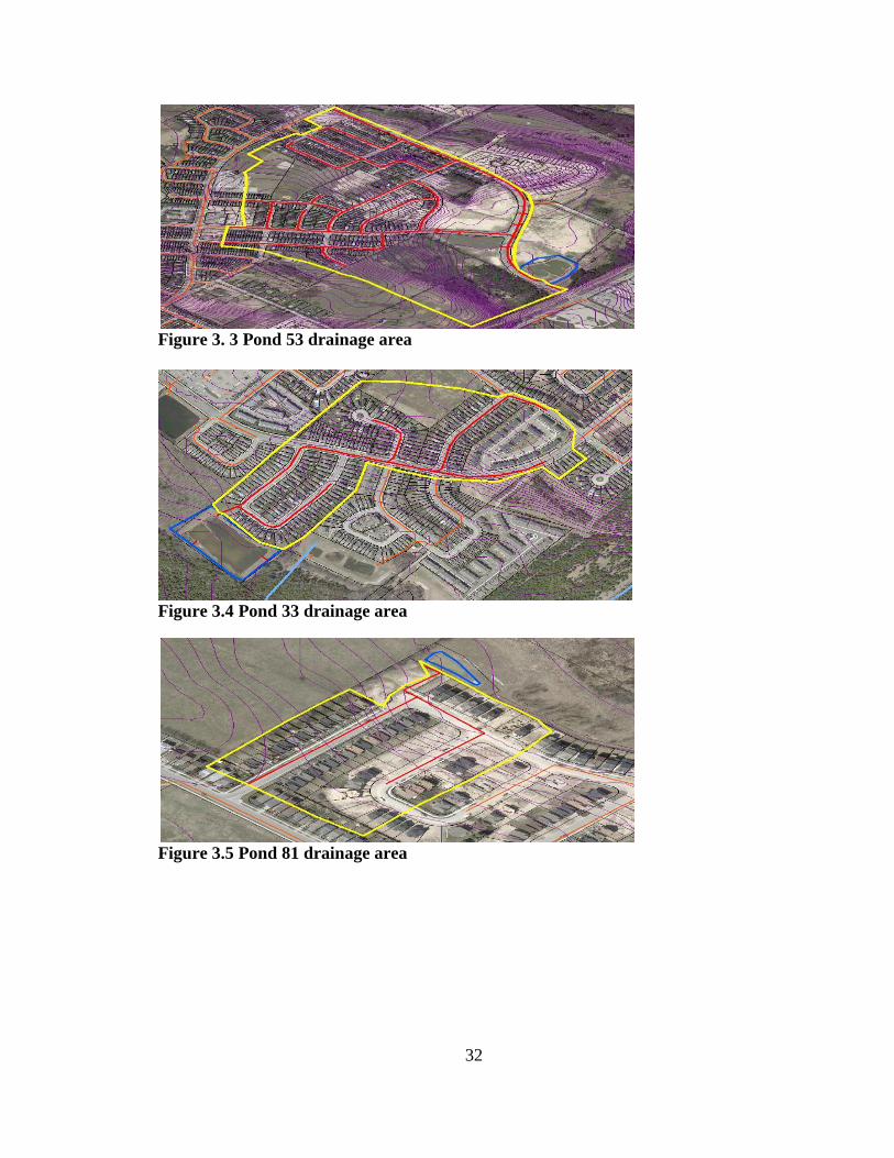
drainage areas are shown in Figures 3.3 through 3.5.
(3.1)
Q = the runoff discharge (m³/s)
Temp = the runoff temperature (°C)
dt = the time increment of 10 minutes
n = the event duration (min)
32
Figure 3. 3 Pond 53 drainage area
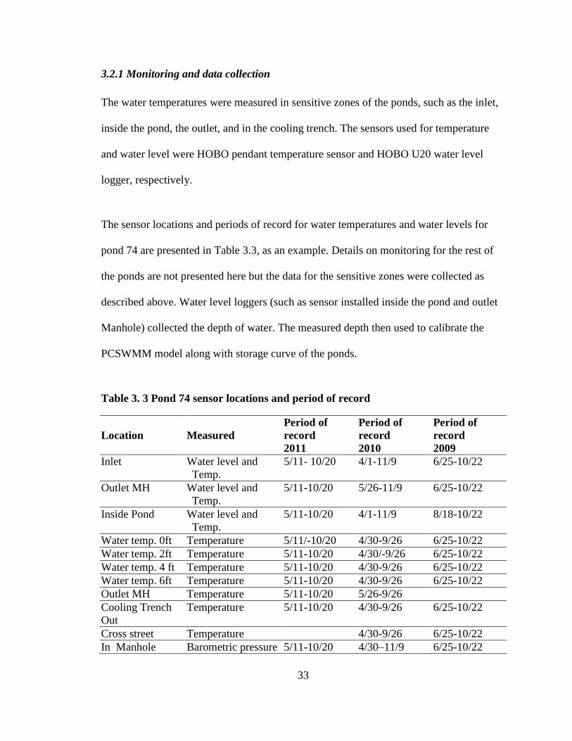
Figure 3.4 Pond 33 drainage area
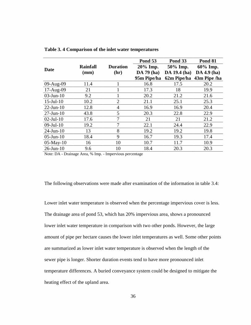
Figure 3.5 Pond 81 drainage area
33
3.2.1 Monitoring and data collection
The water temperatures were measured in sensitive zones of the ponds, such as the inlet,
inside the pond, the outlet, and in the cooling trench. The sensors used for temperature
and water level were HOBO pendant temperature sensor and HOBO U20 water level
logger, respectively.
The sensor locations and periods of record for water temperatures and water levels for
pond 74 are presented in Table 3.3, as an example. Details on monitoring for the rest of
the ponds are not presented here but the data for the sensitive zones were collected as
described above. Water level loggers (such as sensor installed inside the pond and outlet
Manhole) collected the depth of water. The measured depth then used to calibrate the
PCSWMM model along with storage curve of the ponds.
Table 3. 3 Pond 74 sensor locations and period of record
Location Measured
Period of
record
2011
Period of
record
2010
Period of
record
2009
Inlet Water level and
Temp.
5/11- 10/20 4/1-11/9 6/25-10/22
Outlet MH Water level and
Temp.
5/11-10/20 5/26-11/9 6/25-10/22
Inside Pond Water level and
Temp.
5/11-10/20 4/1-11/9 8/18-10/22
Water temp. 0ft Temperature 5/11/-10/20 4/30-9/26 6/25-10/22
Water temp. 2ft Temperature 5/11-10/20 4/30/-9/26 6/25-10/22
Water temp. 4 ft Temperature 5/11-10/20 4/30-9/26 6/25-10/22
Water temp. 6ft Temperature 5/11-10/20 4/30-9/26 6/25-10/22
Outlet MH Temperature 5/11-10/20 5/26-9/26
Cooling Trench
Out
Temperature 5/11-10/20 4/30-9/26 6/25-10/22
Cross street Temperature 4/30-9/26 6/25-10/22
In Manhole Barometric pressure 5/11-10/20 4/30–11/9 6/25-10/22

34
Figure 3.6 shows a typical day’s data for pond 74.
Figure 3.6 Pond 74 data 11 July 2011 rain event
3.3 PCSWMM Modeling
The collected data were used to establish a PCSWMM model to represent the existing
hydrologic conditions of each of the catchments in the Guelph and Kitchener areas. The
land uses within the catchments are varied from pond to pond (residential, parking lot,
combination of residential, and grassland). The drainage areas also vary in size, being
between five and 79 ha. The model was developed from the photogrammetric data and
AutoCAD maps representing the studied areas with the use of GIS tools.
The pond water level data were used to calibrate the PCSWMM model for existing
conditions and the inflow and outflow extracted from PCSWMM was used to calculate
the event mean temperature in different zones of the system, which is inlet, pond water

35
temperature close to outlet, outlet, and cooling trench. Figure 3.7 displays the PCSWMM
results for two events versus the observed values for pond water level.
Figure 3.7 PCSWMM result vs. observed values for pond 53
3.4 Results and Discussions
Section 3.4.1 presents results from a comparison of the inlet water temperatures for the
Guelph ponds. Some discussion about bottom-draw outlet and cooling trenches
performance and effectiveness are presented in section 3.4.2 and 3.4.3.
3.4.1 Land Use Effect on Runoff Temperature
Table 3.4 illustrates twelve rainfall events with different durations.
36
Table 3. 4 Comparison of the inlet water temperatures
Date Rainfall
(mm)
Duration
(hr)
Pond 53 Pond 33 Pond 81
20% Imp.
DA 79 (ha)
95m Pipe/ha
50% Imp.
DA 19.4 (ha)
62m Pipe/ha
60% Imp.
DA 4.9 (ha)
43m Pipe /ha
09-Aug-09 11.4 1 16.8 17.5 20.2
17-Aug-09 21 1 17.3 18 19.9
03-Jun-10 9.2 1 20.2 21.2 21.6
15-Jul-10 10.2 2 21.1 25.1 25.3
22-Jun-10 12.8 4 16.9 16.9 20.4
27-Jun-10 43.8 5 20.3 22.8 22.9
02-Jul-10 17.6 7 21 21 21.2
09-Jul-10 19.2 7 22.1 24.4 22.9
24-Jun-10 13 8 19.2 19.2 19.8
05-Jun-10 18.4 9 16.7 19.3 17.4
05-May-10 16 10 10.7 11.7 10.9
26-Jun-10 9.6 10 18.4 20.3 20.3 Note: DA - Drainage Area, % Imp. - Impervious percentage
The following observations were made after examination of the information in table 3.4:
Lower inlet water temperature is observed when the percentage impervious cover is less.
The drainage area of pond 53, which has 20% impervious area, shows a pronounced
lower inlet water temperature in comparison with two other ponds. However, the large
amount of pipe per hectare causes the lower inlet temperatures as well. Some other points
are summarized as lower inlet water temperature is observed when the length of the
sewer pipe is longer. Shorter duration events tend to have more pronounced inlet
temperature differences. A buried conveyance system could be designed to mitigate the
heating effect of the upland area.

37
3.4.2 Thermal Enrichment in Ponds
Thermal enrichment of all studied ponds is observed in the positive difference of outlet
temperature from inlet temperature as is shown in Tables 3.5 and 3.6, for four ponds. The
outlet Event Mean Temperatures (EMTs) differences from inlet EMTs varied between
1.1 °C to 7.0 °C, which confirms the negative thermal impact of SWM Ponds.
Table 3. 5 Ponds 33 and 53 calculated events mean temperatures.
Date Rainfall
(mm)
EMT
rain
(°C)
Pond 33 EMTs (°C) Pond 53 EMTs (°C)
Inlet Outlet Difference Inlet Outlet Difference
6/08/2010 18.8 12.7 21.4 25.2 3.8 14.6 17.7 3.1
6/16/2010 11.4 13.8 15.1 22.2 7.0 16.0 20.2 4.2
6/27/2010 44.0 22.1 18.0 22.5 4.5 18.5 21.5 3.0
7/23/2010 33.5 25.4 19.5 25.4 5.9 18.4 23.6 5.2
Table 3. 6 Pond 74 and church calculated event mean temperatures.
Date Rainfall
(mm)
EMT
rain
(°C)
Pond 74 EMTs (°C) Pond Church EMTs (°C)
Inlet Outlet Difference Inlet Outlet Difference
7/09/2010 12.8 21.0 22.0 26.4 4.4 20.8 25.1 4.3
7/23/2010 36.2 22.4 20.8 24.7 3.9 19.2 23.8 4.6
8/21/2010 19.2 19.2 21.8 22.9 1.1 20.4 22.9 2.4
9/16/2010 25.8 11.4 14.5 16.7 2.2 15.0 16.2 1.2
3.4.3 Bottom-Draw Outlet Effectiveness
Notable points from observed data and calculated event mean temperature (EMT) for
some events, which are presented in Figure 3.5 and Table 3.7, are as follows:

38
Observed data confirm the cooling effect of the bottom draw outlet for pond 74 in
Kitchener where all ponds have bottom draw outlets.
A significant difference in water temperature was observed between the surface water
temperature and that recorded at 90 cm (3 ft) to 120 cm (4 ft), which can determine the
minimum depth for bottom-draw outlet design.
Figure 3.8 Water temperature at different depths of pond 74
Air temperature went down after event which may cause the graphs to converge. Also,
there was no difference in water temperature at depth for several days which may have
been due to groundwater influence to the bottom of the pond which was not measured for
this study.
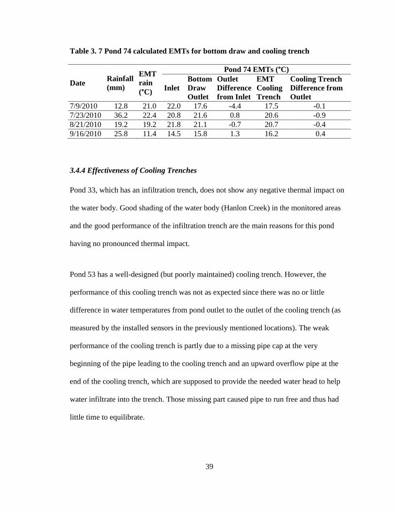
39
Table 3. 7 Pond 74 calculated EMTs for bottom draw and cooling trench
Date Rainfall
(mm)
EMT
rain
(°C)
Pond 74 EMTs (°C)
Inlet
Bottom
Draw
Outlet
Outlet
Difference
from Inlet
EMT
Cooling
Trench
Cooling Trench
Difference from
Outlet
7/9/2010 12.8 21.0 22.0 17.6 -4.4 17.5 -0.1
7/23/2010 36.2 22.4 20.8 21.6 0.8 20.6 -0.9
8/21/2010 19.2 19.2 21.8 21.1 -0.7 20.7 -0.4
9/16/2010 25.8 11.4 14.5 15.8 1.3 16.2 0.4
3.4.4 Effectiveness of Cooling Trenches
Pond 33, which has an infiltration trench, does not show any negative thermal impact on
the water body. Good shading of the water body (Hanlon Creek) in the monitored areas
and the good performance of the infiltration trench are the main reasons for this pond
having no pronounced thermal impact.
Pond 53 has a well-designed (but poorly maintained) cooling trench. However, the
performance of this cooling trench was not as expected since there was no or little
difference in water temperatures from pond outlet to the outlet of the cooling trench (as
measured by the installed sensors in the previously mentioned locations). The weak
performance of the cooling trench is partly due to a missing pipe cap at the very
beginning of the pipe leading to the cooling trench and an upward overflow pipe at the
end of the cooling trench, which are supposed to provide the needed water head to help
water infiltrate into the trench. Those missing part caused pipe to run free and thus had
little time to equilibrate.

40
Pond 81 has an infiltration trench, which shows a cooling effect in dry periods, or
between events, which confirms the effectiveness of contact time between water and
rocks inside the trench. However, no cooling effect was observed during the events. The
main reasons for no cooling effect during the rainfall events were: і) no shading and top
soil cover for the trench; іі) the small volume of the trench which could not hold water to
provide enough contact time for transferring heat from water to rocks and the
surrounding soil; and ііі) the high temperature of the rocks and the initial water in the
cooling trench, both of which are exposed.
Pond 74 has a well performing bottom-draw outlet structure. It was found that the
effectiveness of the bottom draw outlet in driving cooler water to the receiving system is
much greater than the effectiveness of the cooling trench during rainfall events.
Furthermore, the combination of a bottom draw outlet, the cooling trench, and the
interaction with the groundwater may help to give greater performance for this pond, with
no thermal impact on the receiving system during the warm weather of summer.
Pond Church has a very big cooling trench (90 m long) which interacts with ground
water, and is well shaded. As a result, no negative thermal impact was observed during
the course of the study from this cooling trench to the water body.
There are several factors, which influence the effectiveness of cooling trenches, such as
groundwater interaction and the dimensions of the trench. For instance, the ponds 74 and
Church cooling trenches have groundwater interactions. Therefore, the relatively high
efficiency of these cooling trenches may partly result from this interaction. Design

41
aspects of cooling trenches are another important factor on cooling trench performance.
For example, the dimensions of cooling trench of the pond Church are 90 m in the length,
and more than 2 m in the depth, resulting in the best performance of all cooling trenches
studied. Although pond 74 has a big cooling tunnel (60 m long and 2 m deep), less
ground water interaction may result in less cooling effects.
3.5 Conclusions
This study confirms the influence of impervious percentage cover on inlet water
temperature of stormwater management ponds as well as the cooling effect of sewer pipe
systems on inlet water temperature; lower inlet water temperature is observed when the
length of the sewer pipe is greater. Therefore, the presence of a buried conveyance
system partially can mitigate the warming effect of the drainage area.
Thermal enrichment of ponds is confirmed (refer to tables 3.5 and 3.6).
Investigation of the effect of event duration confirms that shorter duration events tend to
have more pronounced inlet temperature changes.
Observed data confirm the cooling effect of the bottom draw outlet; especially when the
depth of bottom draw is 90 cm (3 ft) to 120 cm (4 ft). This can determine the minimum
depth for bottom-draw outlet design.
There are several factors, which influence the effectiveness of cooling trenches, such as
groundwater interaction and the dimensions of the trench. For instance, ponds 74 and
42
Church cooling trenches have groundwater interactions. Therefore, the relatively high
efficiency of these cooling trenches may partly be a result of this interaction. The design
aspects of cooling trenches are another important factor on cooling trench performance.
For example, the pond Church cooling trench dimensions are 90 m long and more than 2
m deep, resulting in the best performance of all cooling trenches studied. Although pond
74 has a big cooling tunnel, 60 m long and 2 m deep, less ground water interactions may
cause less cooling effects from this cooling tunnel. Another important factor in order to
get the best result out of designed and constructed facilities is the maintenance of the
facilities to make sure they are working properly.
In summary, the cooling trench performance is highly dependent on the following
variables:
· Flow rate into the cooling trench;
· Runoff and cooling trench volumes;
· Influent temperature;
· Volume of water in the cooling trench before runoff; and
· Groundwater interaction
3.6 References
Anderson, B., W. Watt, and J. Marsalek. 2002. Critical issues for stormwater ponds:
Learning from a decade of research. Diffuse/Non-point Pollution and Waterhsed
Management, 45(9), 277-283

43
Armour, C. L., 1991. Guidance for evaluating and recommending temperature regimes to
protect fish.
Booth, D. B. and B. P. Bledsoe. 2009. Streams and urbanization. Chapter 6, 93-123.
Herb, W.R., Mohseni, O., Stefan, H.G., 2009. Simulation of temperature mitigation by a
stormwater detention pond. J.Am.Water Resour.Assoc. 45, 1164-1178.
Lieb, D.A., Carline, R.F., 2000. Effects of urban runoff from a detention pond on water
quality, temperature and caged Gammarus minus (Say)(Amphipoda) in a headwater
stream. Hydrobiologia. 441, 107-116.
Marsalek, J., Q. Rochfort, L. Grapentine, and B. Brownlee. 2002. Assessment of
stormwater impacts on an urban stream with a detention pond. Water Science and
Technology, 45(3), 255-264
Picksley, J., and A. Deletic. 1999. Chapter 7: The Thermal Enrichment of Storm Runoff
from Paved Areas-a Statistical Analysis. New Applications in Modeling Urban Water
Systems.
Schueler, T. R., and J. Galli. 1994. Environmental impacts of stormwater ponds.
Watershed Restoration Techniques.
Selong, J. H., T. E. McMahon, A. V. Zale, and F. T. Barrows. 2001. Effect of
temperature on growth and survival of bull trout, with application of an improved method
for determining thermal tolerance in fishes. Transactions of the American Fisheries
Society, 130, 1026-1037
Thompson, A., T. Wilson, J. Norman, A. Gemechu, and A. Roa-Espinosa. 2008.
Modeling the Effect of Summertime Heating on Urban Runoff Temperature1. Journal of
the American Water Resources Association, 44(6), 1548-1563

44
3.7 Appendix to original paper
The original paper to CHI did not include details and the location of sensors nor the
PCSWMM model. For the sense of competence of the thesis information on location of
sensors and PCSWMM model are appended here.
3.7.1 Location of sensors
The locations of the installed sensors in the ponds are illustrated in Figure 3.9. Figure
3.10 and 3.11 are the collected data; water temperature in different parts of the system
including inlet and outlet for summer 2011. There were sensors installed in the ponds to
measure water temperatures at different depths (these are shown in Figure 3.8).

45
Figure 3.9 location of sensors (Triangles are Level loggers and Circles are Pendant
temperature sensors)

46
Figure 3.10 Pond 33 collected data (summer 2011)
Figure 3.11 Pond 53 collected data (summer 2011)

47
The time interval of 10 minutes was used to collect water temperatures data as well as
pond water level. The latter was used to calibrate the PCSWMM model in order to
obtain inlet and outlet flows as discussed in the following. Given the cost and complexity
of flow gauging in storm sewers, this is a reasonable approach.
3.7.2 PCSWMM model
PCSWMM is an urban runoff model and its application is widely acceptable due to the
flexibility of the model. However, some challenges are typically encountered when
modeling the hydrologic response of a catchment (Subhashini et al., 2011). For instance,
groundwater modeling with unknown aquifer properties, modeling subsurface flow using
the simple Groundwater module in PCSWMM, and choosing the appropriate parameters
for model calibration are some well-known challenges when using PCSWMM.
In this study, pond design characteristics were obtained from reports provided by
research partners. In addition, pond sub-catchment characteristics were found using GIS
tools. PCSWMM modeling requires climatologic and catchment topographic data.
Rainfall depths were used as the climatologic inputs in the PCSWMM model.
Climatologic data were collected in Guelph Turfgrass Institute (GTI), and Grand River
Conservation Authority (GRCA) for Guelph and Kitchener, respectively.
An event based modeling approach was used to obtain rainfall-runoff hydrographs from
the PCSWMM model based on the assigned catchment parameters (e.g., drainage area,
average slope, impervious percentage, depression storage). The availability of GIS data

48
for the catchments made the acquisition of data efficient and more efficient. Calibrations
of the model were performed using the collected pond water level data. Manual
calibration was used to get acceptable results with regard to matching the predicted and
measured pond water levels.

49
Chapter 4
Impervious surfaces and sewer pipe effects on stormwater
runoff temperature
This chapter assessed the effect of upland areas on inlet water temperatures of stormwater
management ponds. This chapter is directly from the following published paper:
Impervious surfaces and sewer pipe effects on stormwater runoff temperature
Sabouri, F., Gharabaghi, B., Mahboubi, A., McBean, E. (2013). “Impervious surfaces
and sewer pipe effects on stormwater runoff temperature” Journal of Hydrology 502
(2013) 10-17.

50
Notations
Abbreviation Unit Definition
ANNs - Artificial Neural Networks
AspT °C Asphalt Temperature
CRM - Coefficient of Residual Mass
D hr Duration of Rainfall
DA ha Drainage Area
E - Coefficient of efficiency (Nash-Sutcliffe)
EMT °C Event Mean Temperature
EMTR °C Event Mean Temperature of Rain
EMTI °C Event Mean Temperature of Inlet
GRCA - Grand River Conservation Authority
GTI - Guelph Turf grass Institute
ID - Index of agreement
IMP - Impervious Percentage
MA - Mean Absolute Error
Max - Max Absolute Error
MAPE - Mean Absolute Percentage Error
MI mm/hr Maximum Intensity of Rain
LPL m Longest pipe length
PND m/ha Pipe network density
R mm Rainfall
RMSE - Root Mean Square Error
SCS - Soil Conservation Service
Sn - Normalized Sensitivity Coefficient
SMRE - Square of the Mean Root Error
SWM ponds - Stormwater Mangement Ponds
WEP - Water and Energy Transfer Processes
TES - Thermal Enrichment of Strom-water
TURM - Thermal Urban Runoff Model
MINUHET - Minnesota Urban Heat Export Tool

51
4.1 Introduction
Thermal pollution from urban runoff is a significant contributor to the degradation of
cold-water ecosystems (Boulton 2008; Herb et al. 2008). In addition, water temperature is
one of the most important factors influencing the distribution of aquatic organisms.
Increased temperature and thermal enrichment of a creek or pond can disrupt the aquatic
ecosystem due to thermal shocks harmful to fish such as trout (LeBlance et al. 1997; Lieb
and Carline, 2000). Urbanization can adversely affect stream hydrology as impervious
surfaces may increase the frequency of flood and peak flow rates, sediment loads and
stream temperature (Booth and Bledsoe 2009; Kieser et al. 2003; Nelson and Palmer
2007; LeBlanc 1997; Mohseni et al., 1998, Mohseni and Stefan, 1999).
Galli (1990) reported that the increase in summer stream temperatures in an urban
watershed was related to the degree of imperviousness of the contributing area by a factor
of 0.09oC for every 1% increase in impervious area. Schueler and Galli (1992) reported
stormwater management ponds (SWM ponds) remain the most popular option to control
flooding and to remove suspended solids and contaminants from urban runoff. In
addition, they concluded ponds could produce a diverse array of potential negative
thermal effects on aquatic habitat. Janke et al. (2008) found that heat discharged from
urbanized areas to streams is more sensitive to rain intensity, rainfall duration, and
antecedent pavement temperature. Physical parameters such as slope, roughness, and
length of the paved surface were found to be less influential. Thompson et al. (2008)
52
reported that average asphalt runoff temperature is strongly dependent on initial asphalt
temperature at the start of the rain.
Considerable attention has been given to thermal enrichment of stormwater runoff by
paved surfaces using computer models (Galli 1991; Herb et al. 2009; James and
Verspagen 1996; Janke et al. 2009; Jia et al. 2001; Picksley and Deletic 1999; Thompson,
et al. 2008; Roa-Espinosa et al. 2003; Ul Haq and James 2002; Van Buren et al. 2000;
Xie and James 1993). James and Verspagen (1997) developed the “decade method” to
estimate the temperature of surface runoff from paved surfaces. They reported mean
runoff temperature as a linear function of initial pavement temperature before wetting.
Picksley and Deletic (1999) developed a statistical analysis using graphical observations
of thermal trends, analysis of the event mean temperature (EMT), and analysis of thermal
exponential decay theory. The WEP model (water and energy transfer processes model)
developed by Jia et al. (2002) predicts changes in water and energy budgets associated
with land use changes in urbanized and partially- urbanized watersheds. The TES model
(Thermal Enrichment of Stormwater) developed by Haq and James (2002) is a direct
application of James and Verspagen’s work. The TES model is characterized for a big
difference made in calculation of the Reynolds Number. Herb et al. (2006) developed the
MINnesota Urban Heat Export Tool (MINUHET), which is an analytical model capable
of simulating the flow of stormwater surface runoff and its associated heat content for
small watersheds. The TURM model developed by Roa-Espinosa et al. (2003) is a useful
tool for determining runoff temperature for typical urban areas, although the model is
event based, its major limitation is the rainfall events are treated with uniform intensity as

53
a consequence of using the SCS curve number method for prediction of runoff
hydrographs.
The use and construction of SWM ponds is increasing in the rapidly developing areas of
Ontario and several municipalities have hundreds of SWM ponds. Therefore, the
potential for SWM ponds impacts on receiving streams is significant. This study has been
developed in response to the lack of information regarding the impact of stormwater
management ponds on water temperature; however, it is vital to get a better
understanding of runoff temperature prior to studying the pond’s thermal enrichment. The
main objectives of this paper are to investigate the effect of upland area on runoff
temperature at the inlet of the ponds and to compute a model to predict the runoff
temperature at the inlet of stormwater detention ponds. In this study, the interactions
between rainfall magnitude, rainfall temperature, rainfall intensity, rainfall duration,
drainage area imperviousness, asphalt temperature, and sewer pipe systems are used in
modeling runoff temperature at a SWM pond's inlet. An artificial neural network is
developed as a tool to estimate runoff temperature at the inlet of the stormwater
management ponds during summer times.
4.2. Material and methods
4.2.1 Site selection
Four sub-watersheds with end of pipe control systems or stormwater management ponds
were selected for study. The sites were selected based on accessibility and availability of
design reports. Four sites were chosen: two in the city of Guelph and two in Kitchener as
shown in Figure 4.1.

54
Figure 4.1 Location of Guelph ponds 33 and 53 (left) and Kitchener ponds 74 and
Church (right).
4.2.2 Planning Phase
Five zones were selected for data collection to characterize the thermal enrichment
through all zones, which are: (1) upland area, (2) inlet structure of the pond, (3)
stormwater pond, (4) outlet structure, and (5) receiving water body. The listed locations
of monitor water temperature are recognized as sensitive points since the change of the
water path through the system lead to cooling or warming effect on stormwater runoff.
However, of interest is the effect of upland area on inlet water temperature to the ponds.
Figure 4.2 shows pond 33 catchment areas in Guelph. The drainage area’s boundary
delineation is based on the installed stormwater sewer pipes and catch basins that collect
and divert runoff to the stormwater pond.
Pond catchments vary in size and shape as listed in Table 4.1. Parameters relating to the
studied ponds were collected using GIS, pond reports, and available ponds bathymetry.

55
Table 4.1 Ponds related parameters
Pond Catchment
area (ha) %
Impervious
Impervious
area (ha)
Land use Longest pipe
length(m)
53 79.0 20 15.8 Residential and
empty land 1379
33 19.4 50 9.7 Residential 938
74 35.8 55 19.7 Residential 420
Church 5.1 45 2.3 Parking lot 345
Figure 4.2 Pond 33 watershed in Guelph
4.2.3 Sensor installation and field procedures
Tidbit temperature sensors were used to collect the water temperature during rain events
at ten-minute time intervals. Pond water temperatures and water levels were collected
using HOBO U20 water level loggers at the same time intervals. HOBO software was
used to compensate data and import data to Excel sheets for further analysis when

56
necessary. Meteorological data such as air temperature and precipitation was obtained
from the Guelph Turf grass Institute (GTI) Research Station and the GRCA weather
innovation website.
4.2.4 Event mean temperature calculation
A PCSWMM model was developed to mimic the existing hydrologic conditions of the
catchment areas. The model was developed using AutoCAD maps and GIS tools for
drainage areas. The pond water level data, which was monitored in the course of the
study, were used to calibrate the PCSWMM model for existing conditions. The inflow
time series extracted from PCSWMM and the inlet water temperatures were then used to
calculate the event mean temperature of the inlet (EMTI) using (4.1). Inlet water
temperatures of stormwater ponds were monitored continuously during three summers
(2009, 2010, and 2011) which are used to calculate the EMT of pond's inlet. The Guelph
Turfgrass Institute (GTI) and the Grand River Conservation Authority (GRCA)
monitoring stations provided the required climatic data.
(4.1)
Where Q is the runoff discharge (m³/s), temp is the runoff temperature (°C), dt is the time
increment of 10 minutes, and n is the event duration (min).
The same method was used to calculate the event mean temperature of the rainfall. A
summary of collected data and calculated event mean temperatures are listed in Table
4.2.

57
Table 4.2 Collected data and calculated EMTs

58
Table 4.2 Continue
4.2.5 Overview of ANNs
Artificial neural networks (ANNs) are data processing tools that simulate the structure
and functioning of the human brain. A neural network integrates an interconnected data
processing. Parallel-interconnected data processing can lead to much greater
computational power. This enables ANNs to model complex data even if data are
imprecise and noisy. Over the last several years, ANN modeling has been used in a

59
variety of hydrological and hydraulic phenomena (Chen and Chang, 2009; Kumar, 2012;
Rafiq et al., 2001; Sahoo et al., 2009; Shigidi and Garcia, 2003; Tayfur and Singh, 2005;
Wu and Chau, 2011; Zaghloul and Kiefa, 2001). ANNs have shown great ability in
modeling complex environmental systems with both linear and nonlinear relations.
4.2.6 Design of ANN
In this study an ANN was developed using Tiberius software. In general, neural networks
are trained to perform a task by learning from a set of training instances. After training
and obtaining the new model, there is a need to test the created model to find how
accurate the model is. In this paper, a set of 70 rainfall events captured during three
summers (2009 - 2011) which are used to develop the models.
4.2.7 Feed-Forward Neural Networks
In an ANN with feed-forward topology, information flows only in the direction of inputs
to outputs with no back-loops (Figure 4.3). This task leads ANN to reach the output
accordance to input signals.

60
Figure 4.3 An ANN with its inputs, hidden layers, bias, and output
Training an ANN is crucial to achieving the proper network topology and training
algorithm. Feed-forward neural networks have been the most commonly
used statistical models. The feed-forward processing involves an input layer in which
each input value is multiplied by a corresponding weight. Then, passes the values into the
hidden layer where the model sums the weighted inputs and bias. Finally, the model
passes the sum of all previously weighted inputs and bias by a transfer function to
provide the result to the output layer.
Designing the topology of an ANN entails determining the number of layers and nodes in
each layer. When the topology is built, random weights are given to each link in different
layers, and the training process starts. Once training is done, the network weights are
61
"frozen" and can be used to compute output values for new input samples. The topology
of the network should be modified and the training process restarted.
Back-propagation is a form of supervised training for multi-layer nets, in which the error
data at the output layer is "back-propagated" to update the weights associated to this
layer. Back-propagation algorithms have been widely used as training algorithms in feed-
forward multilayer neural networks (Zaghloul and Kiefa, 2001). In this study, the neural
network topology is designed as a seven-layer training network including an input layer,
hidden layers, and an output layer.
4.3 Results and Discussion
4.3.1 ANN model development
Variables provided by a combination of monitoring, calculation, and use of hydrological
software (PCSWMM) be listed as follows. The depth of rainfall (R, mm), rainfall
duration (D, hr), rain maximum intensity (MI, mm/hr), initial asphalt temperature prior to
rain (AspT, °C), event mean temperature for rain (EMTR, °C), longest pipe length (LPL,
m), impervious percentage (IMP, %), pipe network density (PND, m/ha), and event mean
temperature for inlet (EMTI, °C). EMTI and EMTR both are calculated using (4.1). All
mentioned variables were used to develop an artificial neural network in which EMTR
and LPL found to have greatest relevant importance in the developed model for
predicting the EMTI (case 1). Furthermore, other cases were developed by eliminating
parameters which had either smaller relative importance or not easy to measure. Table
4.3 shows the input parameters for developed artificial neural network models to predict

62
EMTI. There are four developed ANN models named as cases 1 through 4. The
importance of the input variables examined bellow to find the significant influence of
different variables on EMTI. The ANN software, Tiberius, was used to train the data. The
ANN model was first developed with eight inputs as it shown in case 1 of Table 4.3. The
desired output was event mean temperature of the pond's inlet.
Table 4.3 Input parameters for developed ANN models to predict EMTI
Case 1 Case 2 Case 3 Case 4
EMTR EMTR EMTR EMTR
LPL LPL LPL
IMP IMP IMP
PND PND
MI MI
AspT AspT
R
D
4.3.2 Calibration and Validation
The ANN model consisted of eight inputs and seven hidden nodes. In the first approach,
all of data were used to create the predictive model for EMTI to get the overall trend of
the trained network. Then, 70% of the data were randomly selected for training the
network and the rest stood to test the model. According to Legates and McCabe (1999), a
model should include at least one absolute error measure (e.g. RMSE) as a necessary
supplement to a relative error measure. The following measures were used to verify the
model performance. The coefficient of efficiency (CE) (Nash and Sutcliffe, 1970) is
recognized as a good alternative to R². It is a relative error measure, which is sensitive to
differences in the observed and predicted means and variances (Wu and Chau, 2011). The

63
measures of root mean square error (RMSE), the square of the mean root error (SMRE),
maximum absolute error (Max), mean absolute error (MA), mean absolute percentage
error (MAPE), R square, coefficient of efficiency (E), and index of agreement (ID) were
calculated for each data set to describe the predictive capability of the model. RMSE is
frequently used to measure the differences between values predicted by a model or an
estimator and the values actually observed; this measure compares only to the different
forecasting errors within a dataset and not between different ones, as it is scale-
dependent. These individual differences are also called residuals while RMSE serves to
aggregate them into a single measure of predictive power. Two techniques for measuring
error were used in this study named the absolute error and the relative error. The first
indicates how large the error is; the second points to how large the error is relative to the
correct value. The mean absolute percentage error (MAPE), also known as mean absolute
percentage deviation, is a measure of accuracy of a method for constructing fitted time
series values in statistics, specifically in trend estimation. It usually expresses accuracy as
a percentage. Table 4 illustrates the coefficient and different statistical measures for
model evaluation and their range of variability.
Statistical performances are summarized in Table 5, showing the ANN performance for
case 1 to train and test the predictive EMTI. The three ANN models presented in Table 5,
included (1) the overall model using all 106 events for training; (2) The 70 % ANN
model that only used 74 randomly selected events data for training the model; and (3)
used the remaining 30% data (32 events) to test the 70% ANN model. The overtraining of
the ANN model was avoided by using cross validation and early-stopping methods to

64
indicate when further training would not result in better generalization (Tetko et al.,
1995). The cross-validation coefficient was 0.82, which is acceptable. The R² for the 70%
training model was 0.95 and only dropped to 0.90 for the 30% validation test dataset. The
Maximum Absolute Error (MAX) increased slightly from 2.45 for the 70% training
model to 2.61 for the 30% validation test model.
Table 4.6 illustrates a summary of correlation factors either retrieved by ANN software
(Tiberius) or calculated using statistics equations for developed ANN models.
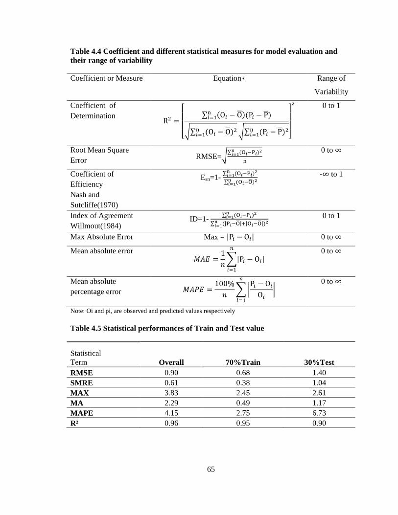
65
Table 4.4 Coefficient and different statistical measures for model evaluation and
their range of variability
Coefficient or Measure Equation∗ Range of
Variability
Coefficient of
Determination
0 to 1
Root Mean Square
Error RMSE=
0 to ∞
Coefficient of
Efficiency
Nash and
Sutcliffe(1970)
Esn=1-
-∞ to 1
Index of Agreement
Willmout(1984) ID=1-
0 to 1
Max Absolute Error Max = 0 to ∞
Mean absolute error
0 to ∞
Mean absolute
percentage error
0 to ∞
Note: Oi and pi, are observed and predicted values respectively
Table 4.5 Statistical performances of Train and Test value
Statistical
Term
Overall
70%Train 30%Test
RMSE 0.90 0.68 1.40
SMRE 0.61 0.38 1.04
MAX 3.83 2.45 2.61
MA 2.29 0.49 1.17
MAPE 4.15 2.75 6.73
R² 0.96 0.95 0.90

66
A comparison of predicted EMTI versus observed EMTI values are illustrated in Figure
4.6.
When comparing the results of all trained ANNs with the calibration set, all the networks
were extremely accurate in their predictions of event mean temperature of the ponds'
inlet. As shown in Figure 4.4, the results of the ANN in prediction of EMTI are presented
for different numbers of input parameters. In the first case, there are eight input
parameters, which are EMTR, LPL, R, D, MI, AspT, and PND. Statistical analyses show
the acceptable range for statistical measures; the importance level of parameters is
discussed in the next section. In the second case, the EMTR was retained as a
representative of rainfall characteristic and magnitude and duration of rainfall were
omitted since. The high level of accuracy (R²=0.94) demonstrates the developed model is
reliable to predict the EMTI. The third case was developed using three inputs (EMTR,
IMP, and LPL); in this case impervious percentage as a known contributor to thermal
enrichment of runoff was retained as well as LPL, which is the representative of the
cooling effect of the buried sewer pipes. R² value related to case three is 0.75, which
shows that the newly developed model has an acceptable predictive availability. The
privilege of the third case is using three parameters, which are easily measurable to
predict the EMTI. In last case, the model developed by using EMTR as the only input
which gives the acceptable statistical measures with R² = 0.70 and ID = 0.97 confirming
predictive capability of this model.

67
Figure 4.4 Artificial Neural Network Predictions of EMTI versus Observed EMTI
Table 4.6 Statistical performance of EMTI models
Case RMSE Max MAE MAPE R² E ID
1 0.90 2.04 0.72 4.15 0.96 0.94 0.99
2 0.88 3.22 0.63 3.38 0.94 0.44 0.82
3 1.14 3.73 0.91 5.30 0.75 0.83 0.95
4 1.59 4.83 1.27 7.28 0.70 0.90 0.97 If all predicted and observed values were the same, then the statistics would yield: Max=0.0, MA=0.0,
MAPE=0.0, RMSE=0.0, R²=1, E=1, and ID=1

68
Trained networks in cases 1 and 2 have the highest measure of R² = 0.96 and 0.94
respectively; case 1 shows a better measure for the index of agreement (ID) and max
absolute error (Max), however, case 2 has the best measure for the root mean square error
(RMSE) among all cases. Model created using Case 4 input variable would be able to
predict the EMTI, when the only available variable is the event mean temperature of
rainfall.
4.3.3 Sensitivity Analysis of the parameters
In order to determine which variable has more influence on EMTI, a sensitivity analysis
was employed. Therefore, the value of each parameter in the developed network of case 1
was perturbed by adding 10%. Table 4.6 illustrates the effect of changing input
parameters on EMTI. The marginal sensitivity coefficient was then determined by the
following equation:
(4.2)
Where Sc is the marginal sensitivity coefficient of the equation, is the change in the
calculated objective function, and is the change in the parameter. Normalizing the
parameters indicates the percent change in the objective function for a 1% change in each
individual parameter. The marginal sensitivity coefficients were normalized to establish
a basis of comparison using the following equation:
∗
(4.3)

69
Where is the normalized sensitivity coefficient, is the expected value of the
perturbed parameter, and is the expected solution. Table 6 shows the sensitivity of the
input parameters in the EMTI for the developed ANN model.
Table 4.1 Sensitivity analysis calculations
Perturbed
Variable EMTR LPL IMP PND
D
AspT
R
MI EMTI Sc Sn
Base 15.5 862.1 37.5 78 18.2 20.4 26.2 16.5 16.8
EMTR 17.7
20.1 1.445 1.275
LPL
850.8
16.7 0.012 0.631
IMP
43.0
17.1 0.193 0.167
PND
84.9 16.4 0.013 0.051
D
20.1 16.9 0.066 0.060
AspT
22.5 16.4 -0.230 -0.217
R
28.8 16.7 -0.057 -0.053
MI
18.1 17.2 0.200 0.180
From these results, the model is determined as most sensitive to change in event mean
temperature of rain; the next levels of importance belonged to longest pipe length,
maximum intensity, and impervious percentage of drainage area, rainfall magnitude,
initial asphalt temperature, pipe network density, and rainfall duration. Table 4.7
illustrates the relative importance of the variables.
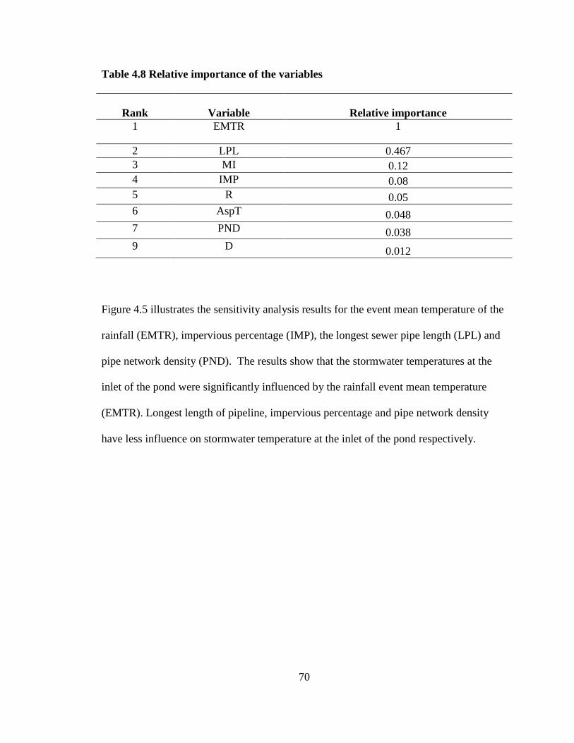
70
Table 4.8 Relative importance of the variables
Rank Variable Relative importance
1 EMTR 1
2 LPL 0.467
3 MI 0.12
4 IMP 0.08
5 R 0.05
6 AspT 0.048
7 PND 0.038
9 D 0.012
Figure 4.5 illustrates the sensitivity analysis results for the event mean temperature of the
rainfall (EMTR), impervious percentage (IMP), the longest sewer pipe length (LPL) and
pipe network density (PND). The results show that the stormwater temperatures at the
inlet of the pond were significantly influenced by the rainfall event mean temperature
(EMTR). Longest length of pipeline, impervious percentage and pipe network density
have less influence on stormwater temperature at the inlet of the pond respectively.
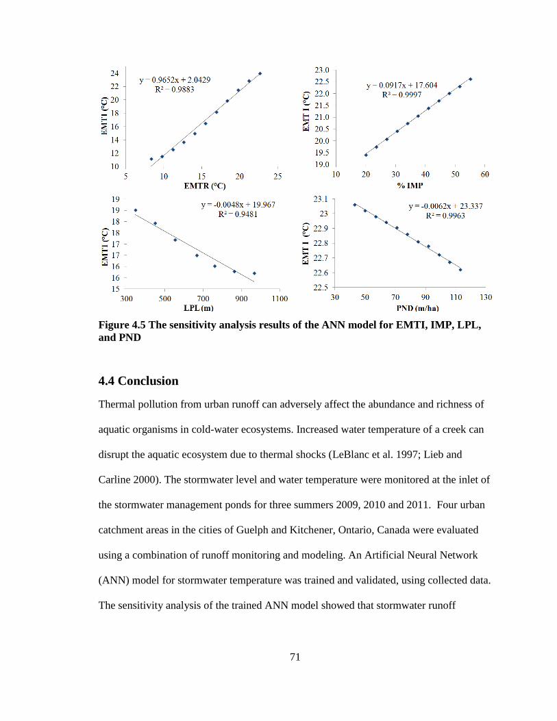
71
Figure 4.5 The sensitivity analysis results of the ANN model for EMTI, IMP, LPL,
and PND
4.4 Conclusion
Thermal pollution from urban runoff can adversely affect the abundance and richness of
aquatic organisms in cold-water ecosystems. Increased water temperature of a creek can
disrupt the aquatic ecosystem due to thermal shocks (LeBlanc et al. 1997; Lieb and
Carline 2000). The stormwater level and water temperature were monitored at the inlet of
the stormwater management ponds for three summers 2009, 2010 and 2011. Four urban
catchment areas in the cities of Guelph and Kitchener, Ontario, Canada were evaluated
using a combination of runoff monitoring and modeling. An Artificial Neural Network
(ANN) model for stormwater temperature was trained and validated, using collected data.
The sensitivity analysis of the trained ANN model showed that stormwater runoff

72
temperatures were most influenced by the following parameters ranked from highest to
lowest sensitivity: EMTR > LPL > MI > IMP > R > AspT > PND > and D, respectively.
Over the last several years, ANN modeling has been used in a variety of complex
hydrological and hydraulic processes. However, there is a lack of information regarding
the use of artificial neural network in modeling urban runoff temperatures. ANNs have
shown great ability in modeling complex environmental systems with both linear and
nonlinear relationships. However, this is the first time that the cooling effect of
underground storm sewer pipes has been investigated and the longest pipe length (LPL)
and sewer pipe network density (PND) are introduced as key input variables to develop a
predictive model for runoff temperature.
The following key points can be concluded from this study:
1- Percent impervious cover of the catchment area (IMP) is the key parameter that
indicates the warming effect of the asphalt and concrete paved surfaces;
sensitivity analyses using the calibrated ANN model demonstrates when IMP was
increased from 20 to 50%, the stormwater temperature increased by 3 °C;
2- Storm sewer pipe’s network density (PND) and longest storm sewer pipe length
(LPL) are the two parameters that control the cooling effect of the underground
storm sewer system. Sensitivity analysis using the calibrated ANN model shows
that when PND increased from 40 to 110, runoff temperature dropped by 0.5 °C,
and when LPL increased from 350 to 970 m, runoff temperature at the outlet
dropped by 2.5 °C. These results show that the storm sewer pipe network can be
designed as a cooling system to compensate for the warming effect of the asphalt
and concrete paved surfaces of the catchment area.

73
3- The forensic sensitivity analysis for the calibrated (trained) ANN model provided
an interesting novel insight on the relative importance of the key engineering
design parameters that influence the discharge temperature to the pond. This
information can lead to improved engineering design guidelines for urban
stormwater management systems discharging to temperature sensitive receiving
systems.
4.8 References
Booth, D.B., Bledsoe, B.P., 2009. Streams and urbanization, the water environment of
cities. USA, Springer, pp. 93-123.
Brierley, P., 2007. Neural Network Software (Tiberius v5.5.0).
http://www.philbrierley.com/phil.html
Chen, Y., Chang, F.J., 2009. Evolutionary artificial neural networks for hydrological
systems forecasting. Journal of Hydrology. 367, 125-137.
Galli, J., 1991. Thermal impacts associated with urbanization and stormwater
management best management practices. Metropolitan Washington Council of
Governments, Maryland Department of Environment, Washington, DC.
Haq, R., James, W., 2002. Thermal enrichment of stream temperature by urban storm
waters. Advances in modeling the management of stromwater impacts. CHI, Guelph,
Canada 5,139- 157.

74
Herb, W., Mohseni, O., Stefan, H., 2007. Heat Export and Runoff Temperature Analysis
for rainfall runoff selection. St. Anthony Falls Laboratory University of Minnesota
Project Report No.483.
Herb, W.R., Janke, B., Mohseni, O., Stefan, H.G., St Paul, M., 2007. Estimation of
Runoff Temperatures and Heat Export from Different Land and Water Surfaces. St.
Anthony Falls Laboratory University of Minnesota Project Report No.488.
Herb, W.R., Janke, B., Mohseni, O., Stefan, H.G., 2008. Thermal pollution of streams by
runoff from paved surfaces. Hydrological Processes. 22, 987-999.
Herb, W.R., Mohseni, O., Stefan, H.G., 2009. Simulation of temperature mitigation by a
stormwater detention pond. Journal of the American Water Resources Associate. 45,
1164-1178.
James, W., Verspagen, B., 1997. Thermal enrichment of stormwater by urban pavement.
Advances in Modeling the Management of Stormwater Impacts CHI, Guelph, Canada. 5,
155-177.
Janke, B.D., Herb, W.R., Mohseni, O., Stefan, H.G., 2009. Simulation of heat export by
rainfall-runoff from a paved surface. Journal of Hydrology. 365, 195-212.
Jia, Y., Ni, G., Kawahara, Y., Suetsugi, T., 2001. Development of WEP model and its
application to an urban watershed. Hydrological Processes 15, 2175- 2194.
Jia Y., NI, G., Yoshitani, J., Kawahara, Y., Kinouchi, T., 2002. Coupling simulation of
water and energy budgets and analysis of urban development impact. Journal of
Hydrologic Eng., ASCE 7 (4), 302- 311.
Kieser, M.S., Fang, A.F., Spoelstra, J.A., 2003. Role of urban stormwater best
management practices in temperature TMDLs. Proceedings of the Water Environment
Federation. 2003, 1716-1739.
75
Kumar, B., 2012. Neural network prediction of bed material load transport. Hydrological
Sciences Journal. 57, 956-966.
LeBlanc, R.T., Brown, R.D., FitzGibbon, J.E., 1997. Modeling the effects of land use
change on the water temperature in unregulated urban streams. Journal of Environmental
Management. 49, 445-469.
Legates, D. R., McCabe, G.,I., 1999. Evaluating the use o f "goodness of fit" measures in
hydrologic and hydroclimatiic model validation. Water Resources Research 35 (1), 223-
241.
Lieb, D.A., Carline, R.F., 2000. Effects of urban runoff from a detention pond on water
quality, temperature and caged Gammarus minus (Say)(Amphipoda) in a headwater
stream. Hydrobiologia. 441, 107-116.
Mohseni, O., Stefan, H.G., 1999. Stream temperature/air temperature relationship: a
physical interpretation. Journal of Hydrology. 218, 128-141.
Mohseni, O., Stefan, H.G., Erickson, T.R., 1998. A nonlinear regression model for
weekly stream temperatures. Water Resources Research. 34, 2685-2692.
Nash, J.E., Sutcliffe,J.V., 1970. river flow forecasting through conceptual models Part I -
A discussion of principles. Journal of Hydrology 10, 282- 290.
Picksley, J.W., Deletic, A., 1999. Thermal enrichment of storm runoff from paved areas-
a statistical analysis. New Applications in Modeling Urban Water Systems. CHI, Guelph,
Canada. 7, 127-138.
Rafiq, M., Bugmann, G., Easterbrook, D., 2001. Neural network design for engineering
applications. Computer and Structures. 79, 1541-1552.
Roa-Espinosa, A., Wilson, T., Norman, J., Johnson, K., 2003. Predicting the impact of
urban development on stream temperature using a Thermal Urban Runoff Model
76
(TURM).Modeling the effect of the natural environment and urban runoff on stream
temperature, 369-389
Sahoo, G., Schladow, S., Reuter, J., 2009. Forecasting stream water temperature using
regression analysis, artificial neural network, and chaotic non-linear dynamic models.
Journal of Hydrology. 378, 325-342.
Schueler, T.R., Galli, J., 1994. Environmental impacts of stormwater ponds. Watershed
Protection Techniques 1(3) 100-111.
Shigidi, A., Garcia, L.A., 2003. Parameter estimation in groundwater hydrology using
artificial neural networks. Journal of Computing in Civil Engineering. 17, 281-289.
Tayfur, G., Singh, V.P., 2005. Predicting longitudinal dispersion coefficient in natural
streams by artificial neural network. Journal of Hydraulic Engineering. 131, 991-1000.
Thompson, A., Wilson, T., Norman, J., Gemechu, A., Roa-Espinosa, A., 2008. Modeling
the effect of summertime heating on urban runoff temperature1. Journal of the American
Water Resources Association. 44, 1548-1563.
Tetko, I.V., Livingstone, D., J., Luik, A.I., 1995. Neural network studies. 1. Comparison
of Overfitting and Overtraining. J. Chem. Inf. Comput.Sci. 35, 826- 833.
Van Buren, M., Watt, W.E., Marsalek, J., Anderson, B., 2000. Thermal enhancement of
stormwater runoff by paved surfaces. Water Research. 34, 1359-1371.
Van Buren, M., Watt, W., Marsalek, J., Anderson, B., 2000. Thermal balance of on-
stream stormwater management pond. Journal of Environmental Engineering. 126, 509-
517.
Willmot, C.J., 1982. Some comments on evaluation of model performance. Bulletin
American Meteorological Society 63 (11), 1309- 1313.

77
Wu, C., Chau, K., 2011. Rainfall–runoff modeling using artificial neural network coupled
with singular spectrum analysis. Journal of Hydrology. 399, 394-409.
Zaghloul, N., Kiefa, A., 2001. Neural network solution of inverse parameters used in the
sensitivity-calibration analyses of the SWMM model simulations. Advances in
Engineering Software. 32, 587-595.

78
Chapter 5
Thermal Design Modeling of Stormwater Management Wet
Ponds
This chapter assessed the effect of design parameters on outlet temperatures of
stormwater management ponds. This chapter is directly from the following submitted
paper to the Journal of Hydrology:
Thermal Design Modeling of Stormwater Management Wet Ponds
Sabouri, F., Gharabaghi, B., Mahboubi, A., McBean, E. (2013). “Thermal Design
Modeling of Stormwater Management Wet Ponds”. Submitted to Journal of
Hydrology.

79
Notations
Abbreviation Unit Definition
ANNs - Artificial Neural Networks
AspT °C Asphalt Temperature
BMPs - Best Management Practices
d m Pond Depth
E - Coefficient of efficiency (Nash-Sutcliffe)
EMT °C Event Mean Temperature
EMTR °C Event Mean Temperature of Rain
EMTI °C Event Mean Temperature of Inlet
EMTO °C Event Mean Temperature of outlet
GRCA - Grand River Conservation Authority
GTI - Guelph Turfgrass Institute
ID - Index of Agreement
MA - Mean Absolute Error
Max - Max Absolute Error
MAPE - Mean Absolute Percentage Error
MI mm/hr Maximum Intensity of Rain
MLP - Multi-layer Perceptron
Q m3/s Runoff Flow Rate
R mm Rainfall Magnitude
RMSE - Root Mean Square Error
SCS - Soil Conservation Service
Sn - Normalized Sensitivity Coefficient
SMRE - Square of the Mean Root Error
SWM ponds - Stormwater Management Ponds
TES - Thermal Enrichment of Strom-water
TPR - Travel Path Ratio
TURM - Thermal Urban Runoff Model
MINUHET - Minnesota Urban Heat Export Tool
VOL m3 Pond Volume
WEP - Water and Energy Transfer Processes

80
5.1 Introduction
Urbanization negatively affects stream hydrology and ecology since increasing
imperviousness through urbanization changes the hydrologic balance in a watershed and
increases frequency of flooding, peak flow of runoff, runoff volume, sediment loadings,
and stream temperatures (Marsalek, 2002; Thompson et al. 2008; Booth, 2009).
Stormwater ponds have been identified as an effective structural best management
practice (BMP) for stormwater quantity and quality control over the past decades, and
have been widely applied across many developed nations (Anderson, 2002). In urbanized
areas, stormwater management ponds are the most adaptable, effective and widely
applied urban best management practices (BMPs) (Schueler and Galli, 1994). Ponds are
probably the most common type of detention used in stormwater management as opposed
to other methods such as wetlands (Starzec et al. 2005). A primary purpose of
stormwater management ponds (SWM ponds ) is to reduce total suspended solids (TSS)
(Persson, 2000) and associated contaminants from urban and industrial surface runoff
during storm events (Anderson, 2002; Marsalek et al., 2002). Ponds also may be used to
mitigate the flooding effects of uncontrolled stormwater runoff on streams; however, they
may also produce a diverse array of negative thermal effects on aquatic habitat (Herb et
al. 2009). Numerous authors (Schueler and Galli, 1994; Marsalek et al. 2002; Ham, et al.
2006; Herb, et al., 2009; Van Buren et al. 2000) have evaluated the environmental effects
of SWM ponds. Schueler and Galli (1994) investigated a series of seven pond design
configurations. They found that the thermal regimes of urban streams tend to be warmer
than for undisturbed catchments. Marsalek et al. (2002) assessed pollution such as heavy

81
metal and polycyclic aromatic hydrocarbons and sediment controls by stormwater
management ponds. They reported that taxa richness and total counts of benthic
organisms did not change much when moving from upstream to downstream of the pond.
Herb, et al. (2009) observed that on average, pond outflow temperature was 1.2 °C higher
than inflow temperature and, indicated that heat energy was added to the runoff from an
asphalt parking lot. They also reported that the rate of heat outflow from the pond is
reduced in response to reductions in ratio of the volumetric outflow rate to inflow rate; as
a result, although the duration of impacts increased, temperature impacts to a receiving
system were reduced.
According to Van Buren et al. (2000), assuming a completely mixed condition, the
average pond water temperatures are a function of thermal energy stored in the pond. To
reduce the thermal effect of stormwater management ponds on receiving waterbodies,
techniques such as, night-time release, use of shading, cooling or infiltration trenches,
and bottom draw outlets may assist. Recorded data from a pond in Kingston, Ontario
showed surface water was 3.6 °C warmer than the average temperature recorded at the
bottom of the pond at 0.9 m. (Van Buren et al. 2000).
This study has developed in response to a lack of sufficient information and data in
Ontario with respect to potential adverse thermal enrichment effects of SWM ponds on
sensitive aquatic habitat. Both monitoring and modeling methods are employed to
evaluate the effect of alternative SWM pond designs on stormwater pond released
temperatures and to estimate the water temperature at the outlet of stormwater

82
management ponds. The main objective is to estimate thermal enrichment of the
stormwater management pond corresponding to the rain events. This is accomplished by
a comparative analysis of observed water temperature in different parts of the system and
development of a model to predict pond’s outlet water temperature as a function of pond
design parameters and precipitation characteristics, such as pond’s inlet water
temperature, pond volume, pond depth, travel path ratio, magnitude of rainfall, and
rainfall event mean temperature.
5.2 Material and methods
5.2.1 Site description
Four urban sub-watersheds with stormwater management ponds were selected for study.
The sites were selected based on accessibility and availability of design reports to collect
a broad range of data for different design components. Two ponds were studied in each of
the cities of Guelph and Kitchener and monitored during three summers (2009- 2011) to
calculate event mean temperature of the pond inlets (EMTI) and outlets (EMTO). Design
parameters for the ponds are listed in Table 1. It is worth noting that Ponds 33 and
Church were very shallow with average depths less than 0.5 m and very large relative
surface area (Ratio of Pond Surface Area to Catchment Area) of 4%, while the other two
ponds 53 and 74 were deeper ponds with smaller relative surface area of only 1% as
shown in Table 5.1.

83
Table 5.1 Design parameters for the selected ponds
Pond Catchment
area (ha)
Volume
(m³)
Surface
Area
(m²)
Average
Depth (m)
Ratio of Pond
Surface Area to
Catchment
Area
Travel Path
Ratio (-)
33 19.4 4000 6800 0.48 0.035 0.7
53 79.0 6440 8400 0.95 0.011 1.1
74 35.8 5376 4000 1.34 0.011 1.4
Church 05.1 950 2165 0.44 0.042 1.6
Travel path ratio (TPR) is defined as the ratio of the most likely travel path of runoff
through the pond (from inlet to outlet) to the longest path that water can take from inlet to
outlet; the longest distance is considered as the summation of the two main pond
dimensions. TPR first was developed by Orozco and Cleveland, 2007 as a measure of
Short-Circuiting potential in stormwater basins. TPR is employed as many ponds were
designed based on adherence of desired length-to-width ratio according to guidelines.
The effect of inlet location related to outlet was based on TPR criterion to account for the
relative position of inlet and outlet as well as baffles (Orozco and Cleveland, 2007).
5.2.1.1 Monitoring equipment and data collection
The monitoring program included instrumentation designs and installation tools to
measure and record water level and water temperature at the inlet and outlet of the ponds.
Water temperature sensors were installed at incremental depths. Onset and Hobo U20
level loggers as well as pendant and Tidbit temperature probes were used to measure
water levels and water temperatures, respectively. Hobo software was used to
compensate water level data and import to Excel when collected data transferred from
sensors to HOBO waterproof shuttle. Hydrometeorological data such as air temperature,

84
and relative humidity were obtained from Elora Research Station and Grand River
Conservation Authority (GRCA) for the cities of Guelph and Cambridge.
Pond 33
This pond with a contributing area of 19.4 ha is located in the City of Guelph, South
Creek Trail, next to Preservation Park (Latitude 43.50953, longitude -80.21835). A pond
inlet forebay had been constructed to retain the larger sediment particles. The forebay
was designed with 2:1 length/width ratio, 1.2 m maximum depth and 7:1 side slopes. The
total forebay volume and permanent pool are 1500 and 4000 m3 respectively. All flows
up to the five-year rainfall event discharge through the quality control outlet structure.
According to the report provided by the City of Guelph Works Department, the pond
quality outlet is designed to detain the “first flush” 25 mm rainfall event for a minimum
of 24 hours. The flow rates from the quality outlet structure are controlled by a 200 mm
diameter outlet pipe. Both the quality and quantity outlets from the pond discharge to
riprap dispersion structures prior to discharging to a receiving system (City of Guelph
Works Department, 1996).
Pond 53 Pond 53 is located in the City of Guelph at the intersection of York and Watson streets
(Latitude 43.56326, longitude -80.21019) with a contributing area of 79 ha draining to
Clythe Creek. Clythe Creek is located south of the site and eventually discharges into the
Eramosa River downstream of York Road. The facility outlet structure consists of a fully
perforated riser with an orifice plate set at different levels to release the water over a
minimum of 24 hours. The water quality extended detention discharge from the orifice is
released to a cooling trench before entering Clythe Creek.

85
Figure 5.1. Ponds 33 (left) and 53 (right) and location of sensors
Note: The circles represent; Pendant or Tidbit temperature probes and the triangles
represent the location of U- 20 Hobo water level data loggers.
Pond 74
Pond 74 is located at the northwest corner of the intersection of Bleams Road and
Fischer – Hallman Road, Kitchener (Latitude 43.38921, longitude -80.46751). The
drainage area of the pond is 35.8 ha; water quality and erosion control provided through a
forebay. The outlet structure discharges directly to an extension of the existing culvert.
The outlet structure contains orifices intended to control the discharge from different
sizes of storms. A bottom-draw outlet structure allows cooler water to discharge from the
bottom of the pond (MTE, 2004).
"Church" pond
The so-called Church pond is located west of Strasburg Road and southeast of Huron
Road in the City of Kitchener (Latitude 43.38921, longitude -80.46751). The drainage
area for this pond is 5.14 ha. The forebay is separated from the main pond area by a
berm/weir, isolating the more turbulent inlet zone from the fine-particle settling and
outlet zone. The water quality extended detention discharge from the orifice is released to
a cooling trench.
Outlet
Inlet Outlet
Inlet
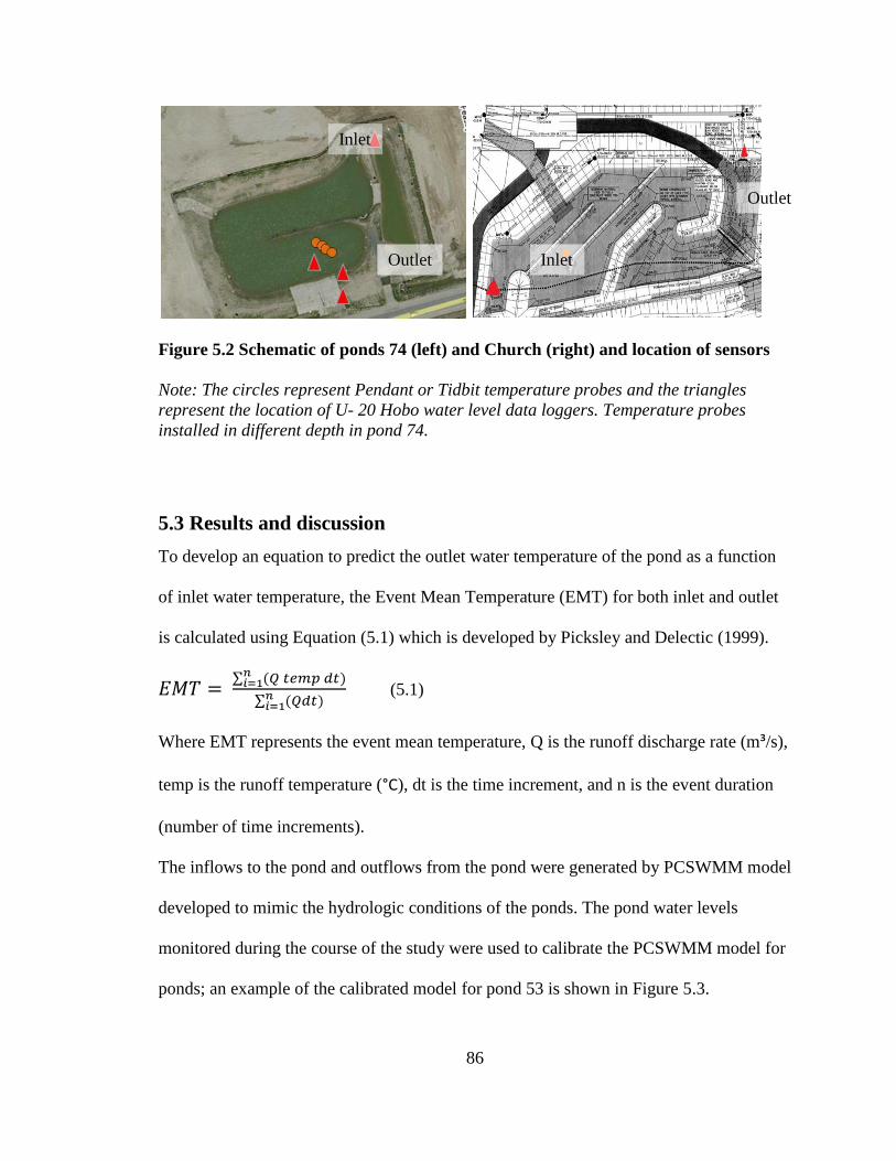
86
Figure 5.2 Schematic of ponds 74 (left) and Church (right) and location of sensors
Note: The circles represent Pendant or Tidbit temperature probes and the triangles
represent the location of U- 20 Hobo water level data loggers. Temperature probes
installed in different depth in pond 74.
5.3 Results and discussion
To develop an equation to predict the outlet water temperature of the pond as a function
of inlet water temperature, the Event Mean Temperature (EMT) for both inlet and outlet
is calculated using Equation (5.1) which is developed by Picksley and Delectic (1999).
(5.1)
Where EMT represents the event mean temperature, Q is the runoff discharge rate (m³/s),
temp is the runoff temperature (°C), dt is the time increment, and n is the event duration
(number of time increments).
The inflows to the pond and outflows from the pond were generated by PCSWMM model
developed to mimic the hydrologic conditions of the ponds. The pond water levels
monitored during the course of the study were used to calibrate the PCSWMM model for
ponds; an example of the calibrated model for pond 53 is shown in Figure 5.3.
Inlet
Outlet Inlet
Outlet

87
Figure 5.3 PCSWMM model simulations for pond 53
Predicted water level time series (red line) versus observed pond water level (green line)
during the June 19th to July 5th, 2010 events.
5.3.1 Thermal Enrichment in Ponds
Thermal enrichments for the monitored ponds are listed in Table 5.2 and Table 5.3. The
EMTO’s differ from EMTI by 3 °C to 10.6 °C in Table 5.3, and confirm the thermal
effects of Ponds 33 and 53.

88
Table 5.2 Ponds 33 and 53 calculated events mean temperatures
Date Rainfall
(mm)
Pond 33 EMTs (°C) Pond 53 EMTs (°C)
Inlet Outlet Difference Inlet Outlet Difference
7/11/2009 13.4 19.6 23.4 3.8 18.9 23.4 4.5
7/20/2009 46.8 18.6 22.3 3.7 17.3 21.4 4.1
8/8/2009 27.0 20.4 24.6 4.2 19.4 22.5 3.1
6/9/2010 18.8 15.4 25.2 9.8 14.6 17.7 3.1
6/16/2010 11.4 15.2 22.2 7.0 16.0 20.2 4.2
6/27/2010 37.8 18.0 22.5 4.5 18.5 21.6 3.0
7/9/2010 19.6 18.3 25.9 7.6 18.2 25.0 6.8
7/23/2010 46.5 19.5 25.3 5.8 18.4 23.6 5.2
6/3/2011 24.6 11.7 21.1 9.5 11.3 18.8 7.5
6/6/2011 37.6 16.1 25.0 8.9 13.9 20.3 6.4
6/21/2011 30.8 13.0 21.8 8.8 14.7 21.8 7.2
7/2/2011 16.2 13.7 24.3 10.6 13.9 23.3 9.4
8/13/2011 16.4 16.1 26.0 9.9 18.8 24.1 5.3
Average - 16.6 23.8 7.2 16.5 21.8 5.4
Note: 48 hours drawdown time considered and event separated accordingly. Difference
are calculated as outlet EMTs minus inlet EMTs.
Pond 33 discharges water to a cooling trench from a shallow bottom draw and pond 53
discharges water to the receiving system through a perforated pipe as opposed to pond
74, which has a bottom, draw outlet to direct the stormwater to an outlet manhole from
the bottom of the pond at a depth of 4 m. As seen from the calculated values in Table 5.3,
the average thermal effect of pond 74 for all events was 0.9 °C, which confirms the
importance of bottom-draw outlet to mitigate the thermal effects of stormwater
management ponds. However, there may be other factors, which could have contributed
to the minimal thermal effect of pond 74, as compare to other ponds studied here. One
identified factor is the influence of groundwater. This was suggested by the overall lower
temperature of pond 74, as would be expected from groundwater fed pond. This is also

89
supported by observations by MTE report (2004). The average increase in temperature
(i.e. the thermal impact) of ponds Church, 33 and 53 were 3.7 °C, 7.2 °C, and 5.4 °C,
respectively. Table 5.3 indicates that without the bottom draw, the thermal impacts to the
receiving systems are much greater as opposed to when there is a bottom draw outlet.
Table 5.3 Pond 74 and Church calculated event mean temperatures
Date Rainfall
(mm)
Pond 74 EMTs (°C) Pond Church EMTs (°C)
Inlet Outlet Difference Inlet Outlet Difference
6/11/2009 12.8 18.5 18.8 0.3 19.24 21.3 2.1
8/4/2009 36.4 20.8 20.0 -0.7 20.7 25.4 4.8
8/8/2009 30.2 20.2 19.7 -0.5 21.2 24.1 2.9
8/20/2009 59.6 21.1 18.5 -2.6 20.0 24.4 4.4
6/9/2010 32.2 22.0 26.4 4.4 20.8 25.8 5.0
6/22/2010 36.2 20.8 24.7 3.9 18.2 25.6 6.4
8/8/2010 08.4 21.6 23.5 1.9 19.9 23.6 3.8
8/21/2010 23.8 21.8 22.9 1.1 20.4 22.2 1.8
9/2/2010 27.2 19.8 22.7 2.9 17.1 22.0 4.9
9/16/2010 25.8 14.5 16.7 2.2 15.0 15.5 0.5
6/4/2011 18.6 14.5 15.9 1.4 15.3 21.3 6.0
6/22/2011 33.4 17.9 17.7 -0.2 17.5 22.0 4.5
8/14/2011 15.6 19.1 19.1 0.0 19.9 22.7 2.8
8/24/2011 21.6 20.8 19.7 -1.1 20.7 22.8 2.0 Average 19.5 20.5 0.9 19.0 22.8 3.7
Note: 48 hours drawdown time considered and event separated accordingly.
The minimum depth for a bottom-draw outlet to be effective and compensate the
warming effect of a pond (the warming effect of a SWM ponds estimate to be 5 °C
according to MOE guideline 2003) is reported as 90 to 120 cm (Sabouri et al. 2012). The
significant difference (about 5 °C) in water temperatures observed between the surface
water temperature and that of depths between 90 and 120 cm. Figure 5.4 presents water
temperature profiles during the Aug. 2nd
to 5th
, 2010 dry weather highlighting the effects
of depth on water temperature. The largest decreases in water temperature occur when

90
depth increases from zero to 1.2 m, therefore ponds deeper that 1.2 m would benefit the
most from discharging cooler water. The peak for water temperatures estimate to be
happen at 3:00 p.m. according to the observed collected water temperatures data,
therefore, water temperatures at 3:00 p.m. are used to create the graph.
Figure 5.4 Pond water temperature profiles during the Aug. 2nd
to 5th
, 2010 dry
weather
5.3.2 Ponds outlet temperature prediction using Artificial Neural Network (ANN)
Artificial Neural Network (ANN) has been successfully used in the discipline of
hydrology and water resources to model relations such as rainfall runoff processes,
prediction of daily stream flows, and forecasting water quality parameters (e.g. Chen and
Chang 2009, Kumar et al. 2012). This study makes use of the ability of ANN for
mapping complex nonlinear relations to approximate the pond’s outlet water temperature

91
for rainfall events. Several types of ANN exist, of which the most popular is the feed-
forward multi-layer perceptron (MLP) which is used in this research.
In order to choose the input variables to develop the ANN model, key storm events and
pond design parameters are considered and named case 1 as shown in Table 5.4 and 5.5.
Key storm event variables include depth of rainfall (R, mm), event mean temperature for
rainfall (EMTR, °C), event mean temperature for runoff at pond inlet (EMTI, °C); and
pond design parameters consist of travel path ratio (TPR), pond volume (VOL, m³), and
average pond depth (d, m). Surface area of the pond is not included since it can be
calculated using two other parameters (volume, average depth) and surface area of the
pond is not an independent variable in the model. All mentioned variables were used to
develop an ANN in which EMTI and TPR were found to have greatest relative
importance in the developed model for predicting the EMTO (case 1). Furthermore, other
cases of ANN were developed by eliminating parameters, which had smaller relative
importance according to statistical analyses. Table 5.4 illustrates the level of importance
of variables used to develop ANN models. In all cases the model is most sensitive to
EMTI; the next levels of importance belonged to TPR, EMTR, VOL, R and d,
respectively. Table 5.5 shows all the input parameters for developed ANN models to
predict EMTO.
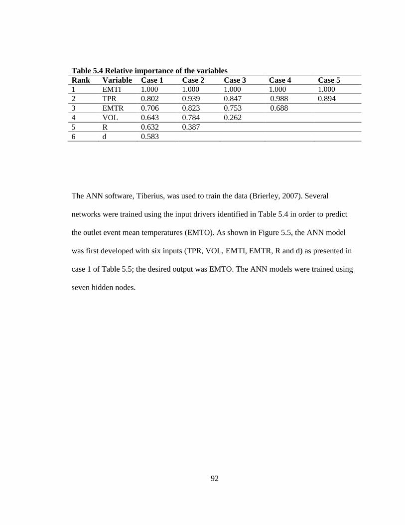
92
Table 5.4 Relative importance of the variables
Rank Variable Case 1 Case 2 Case 3 Case 4 Case 5
1 EMTI 1.000 1.000 1.000 1.000 1.000
2 TPR 0.802 0.939 0.847 0.988 0.894
3 EMTR 0.706 0.823 0.753 0.688
4 VOL 0.643 0.784 0.262
5 R 0.632 0.387
6 d 0.583
The ANN software, Tiberius, was used to train the data (Brierley, 2007). Several
networks were trained using the input drivers identified in Table 5.4 in order to predict
the outlet event mean temperatures (EMTO). As shown in Figure 5.5, the ANN model
was first developed with six inputs (TPR, VOL, EMTI, EMTR, R and d) as presented in
case 1 of Table 5.5; the desired output was EMTO. The ANN models were trained using
seven hidden nodes.

93
Figure 5.5 The ANN Model consist of input layer, hidden layers, and output layer
Five cases were identified to develop ANN models to predict the EMTO. Case 1 input
variables included EMTR, TPR, EMTR VOL, R, and d. Variables showing the lowest
level of importance in each case were omitted (according to statistical analyses) and
other cases (2 through 5) were created and used to develop the ANN models. An
exception though goes to case 4, since design parameters (TPR, VOL and d) are excluded
to determine the effect of these parameters.

94
Table 5.5 Input parameters for developed ANN models to predict EMTO
Case 1 Case 2 Case 3 Case 4 Case 5
EMTI EMTI EMTI EMTI EMTI
TPR TPR TPR R TPR
EMTR EMTR EMTR EMTR
VOL VOL VOL
R R
d
A comparison of predicted EMTO versus observed EMTO values between case 1 and
case 4 is illustrated in Figure 5.6. When comparing the results of all trained ANNs with
the calibration set, R² varied from 0.99 to 0.62, which demonstrates a good level of
accuracy of prediction.

95
Figure 5.6 Comparison of observed EMTO and predicted EMTO for two cases
(a) Full model with six input parameters (TPR, VOL, d, EMTI, R, and EMTR) versus
(b) Model with only three input parameters (EMTI, R, and EMTR).
Shown in Figure 5.6 are the results of ANN prediction of EMTO presented for case 1 and
case 4 which have different numbers of input parameters. In the first case, there are six
input parameters: EMTI, TPR, EMTR, VOL, R (rain), and d. Moreover, the developed
model has a R² of 0.99. In the second case, the depth of pond omitted and developed
model shows the R² of 0.85. The third case was developed using four variables, which
were EMTI, TPR, EMTR, and VOL with R² of 0.65. In case 4, an ANN model was
developed using only three input variables (EMTI, R and EMTR) which are not design

96
parameters, a R² of 0.77 is obtained for this model; and the fifth case was developed
using two inputs (EMTI and TPR) with R² of 0.62.
The 6-parameter model was able to explain 99% of the variability in the observed mean
event temperatures at the pond outlet; however, the 3-parameter model could only
account for 77% of the variability. However, it shows that TPR, d, and VOL which are
design parameters account for 22% of the variability. Design parameters (TPR, d, VOL)
control by the design’s engineer, therefore, they could govern and improve the
constructive strategy of the facility.
5.3.3 Training and Evaluation of the ANN Model
The ANN model (Case 1) consisted of six inputs and seven hidden nodes. About 70% of
data were randomly selected for training of the network and the remainder were used for
testing the accuracy of the model. Table 5.6 illustrates the coefficients and different
statistical measures for the ANN model evaluation and their range of variability.

97
Table 5.6 Statistical measures for model evaluation and their range of variability
Coefficient or Measure Equation∗ Range of
Variability
Coefficient of
Determination
0 to 1
Root Mean Square
Error RMSE=
0 to ∞
Coefficient of
Efficiency
Nash and
Sutcliffe(1970)
Esn=1-
-∞ to 1
Index of Agreement
Willmout(1984) ID=1-
0 to 1
Max Absolute Error Max = 0 to ∞
Mean absolute error
0 to ∞
Mean absolute
percentage error
0 to ∞
Note: Oi and pi, are observed and predicted values respectively

98
Table 5.7 Statistical performances of train and test value
Statistical
Term
Overall
Performance
70% Dataset
Used for Training
30% Dataset
Used for Testing
R² 0.99 0.94 0.99
RMSE 0.12 0.08 1.56
Esn 0.92 0.89 0.93
ID 0.97 0.94 0.95
MAX 0.47 0.24 4.30
MAE 0.09 0.04 1.06
MAPE 0.42 0.98 4.47
Statistical performance of the ANN model (Case 1 – with 6 input parameters) for both the
training as well as for testing data sets are summarized in Table 5.7, showing the ANN
performance for case 1 to train and test the prediction of EMTO.
5.3.4 Sensitivity analysis of the parameters
Figure 5.7 presents the sensitivity analyses of the trained ANN model; this analysis
revealed that increasing pond volumes from 2000 to 4000 m3 resulted in an average
increase of 0.5°C in the EMTO – assuming all other factors remain constant. The rate of
solar radiation absorbed by the pond is related to pond surface area. Since pond volume
and pond surface area are highly related,it is highly likelythat increasing the volume of
the pond will result in an increased EMTO. Also, increasing the travel path ratio from
0.6 to 1.2 resulted in an average increase of 6 °C in EMTO. Both larger volume ponds
and ponds with elongated travel paths tend to discharge more of the warmer water that
has been sitting in the pond, rather than the cooler runoff water from a fresh event.
However, increasing average pond depth from 0.6 to 1.0 m, in the model results in a

99
decrease of up to 9 °C in EMTO, which is in agreement with the observed data.
Comparison of surface water temperature with water temperature at depth of 1m is shown
in Figure 5.4.
Figure 5.7 ANN model sensitivity analysis of EMTO to pond key design parameters
5.4 Conclusion
An Artificial Neural Network (ANN) model trained using monitoring data explain 99%
of the variability in the event mean temperatures at the pond outflow (EMTO). The input
variables to develop the ANNs was chosen based on two categories that consist of key
storm event parameters (EMTI, EMTR, R) and design parameters (TPR, VOL, d).

100
In the late spring and summer months, water that is sitting in the typically shallow wet
ponds is generally warmer than fresh event runoff temperature entering the pond. The
average event mean temperatures at the pond outflow (EMTO) was 5.4 °C warmer than
the average event mean temperatures at the pond inlet (EMTI) for the monitored storms.
Concerning key design parameters of stormwater ponds, larger permanent pool volumes
tend to release the warmer water resident in the ponds. Increasing travel path ratio using
baffles can lead to less mixing of the water that is resident in the pond with the cooler
fresh event runoff and therefore an increase in event mean temperature of outlet (EMTO).
Increasing pond volume from 2000 to 4000 m³ - while keeping all other parameters
constant - results in an average increase of 5 °C in EMTO; increasing travel path ratio
from 0.6 to 1.2 leads to an average increase of 6 °C in EMTO. Hence, larger volume
ponds and ponds with elongated travel path tend to discharge more of the warmer water
that is sitting in the pond rather than the cooler, fresh event runoff. However, the
increasing average pond depth from 0.6 to 1.0 m, in the model, results in an average
decrease of 9 °C in EMTO; therefore, design of ponds with average depths greater than
1.2 m can result in significant decreases in EMTO using bottom-draw structures.

101
5.5 References
Ackerman, D., Stein, E., 2008. Evaluating the Effectiveness of Best Management
Practices Using Dynamic Modeling. Journal of Environmet Engineering. 134, 628-639.
Anderson, B., Watt, W., Marsalek, J., 2002. Critical issues for stormwater ponds:
Learning from a decade of research. Diffuse/Non-point Pollution and Watersheds
Management. 45, 277-283.
Armour, C.L., 1991. Guidance for evaluating and recommending temperature regimes to
protect fish, US Dept. of the Interior, Fish and Wildlife Service.
Backstrom, M., Viklander, M., 2000. Integrated stormwater management in cold
climates. Journal of Environtal Science Health-Toxic Hazardous Substances and
Environmental Engineering. no.8., 1237.
Bogan, T., Mohseni, O., Stefan, H.G., 2003. Stream temperature-equilibrium temperature
relationship. Water Resources Research. 39, 7.1-7.12.
Bogan, T., Stefan, H.G., Mohseni, O., 2004. Imprints of secondary heat sources on the
stream temperature/equilibrium temperature relationship. Water Resources Research. 40,
W12510.
Booth, D.B., Bledsoe, B.P., 2009. Streams and urbanization, the water environment of
cities. USA, Springer, pp. 93-123.
Booth, D.B., 1991. Urbanization and the natural drainage system—impacts, solutions,
and prognoses. The institute for environmental studies. 7.
Booth, D.B., Jackson, C.R., 1997. Urbanization of aquatic systems: degradation
thresholds, stormwater detection, and the limits of mitigation. Journal of American Water
Resources Association. 33, 1077-1090.

102
Brierley, P., 2007. Neural Network Software (Tiberius v5.5.0).
http://www.philbrierley.com/phil.html
Brun, S., Band, L., 2000. Simulating runoff behavior in an urbanizing watershed.
Computer, Environment and Urban Systems.. 24, 5-22.
Cathcart, T.P., Wheaton, F.W., 1987. Modeling temperature distribution in freshwater
ponds. Aquaculture Engineering. 6, 237-257.
Cherry, D., Dickson, K.L.J., Stauffer, J., 1977. Preferred, avoided, and lethal
temperatures of fish during rising temperature conditions. Journal of the Fisheries
Research Board of Canada. 34, 239-246.
Chen, Y., Chang, F.J., 2009. Evolutionary artificial neural networks for hydrological
systems forecasting. Journal of Hydrology. 367, 125-137.
Cox, M., Bolte, J., 2007. A spatially explicit network-based model for estimating stream
temperature distribution. Environmental Modelling and Software. 22, 502-514.
Creaser, C.W., 1930. Relative importance of hydrogen-ion concentration, temperature,
dissolved oxygen, and carbon-dioxide tension, on habitat selection by brook-trout.
Ecology., 246-262.
Davidson, B., Bradshaw, R., 1967. Thermal pollution of water systems. Environmental
Science Technology. 1, 618-630.
Dingman, S.L., 1972. Equilibrium temperatures of water surfaces as related to air
temperature and solar radiation. Water Resources Research. 8, 42-49.
Eaton, J., McCormick, J., Goodno, B., O'brien, D., Stefany, H., Hondzo, M., et al., 1995.
A field information-based system for estimating fish temperature tolerances. Fisheries.
20, 10-18.

103
Fang, X., Stefan, H.G., 1996. Dynamics of heat exchange between sediment and water.
Water Resources Research. 32, 1719-1727.
Farr, D., 2008. Sustainable urbanism : urban design with nature, Hoboken, N.J., Wiley.
Fennessey, L.A.J., Hamlett, J.M., Aron, G., LaSota, D., 2001. Changes in runoff due to
stormwater management pond regulations. Journal of Hydrologic Engineering. 6, 317.
Ford, D.E., Stefan, H.G., 1980. Thermal prediction using integral energy model. Journal
of Hydraulics Division., 39-55.
Galli, J., 1991. Thermal impacts associated with urbanization and stormwater
management best management practices. Metropolitan washington council of
governments, maryland department of environment, washington, DC.
Gao, J., Merrick, N.P., 1996. Simulation of temperature and salinity in a fully mixed
pond. Environment Software. 11, 173-178.
Ham, J., Toran, L., 2006. Effect of upstream ponds on stream temperature. Journal of
Environmental Geology. 50, 55-61.
Hedberg, T., 1999. Attitudes to traditional and alternative sustainable sanitary systems.
Water Science and Technology. 39, 9-16.
Herb, W.R., Mohseni, O., Stefan, H.G., 2009. Simulation of temperature mitigation by a
stormwater detention pond. Journal of the American Water Resources Association. 45,
1164-1178.
Hossain, M., Alam, M., Yonge, D.R., Dutta, P., 2005. Efficiency and flow regime of a
highway stormwater detention Pond in washington, USA. Water, Air, Soil Pollution. 164,
79-89.
Janke, B.D., Herb, W.R., Mohseni, O., Stefan, H.G., 2009. Simulation of heat export by
rainfall-runoff from a paved surface. Journal of Hydrology. 365, 195-212.

104
Kehl, O., Wichern, M., Lübken, M., Horn, H., 2009. Analysis of design approaches for
stabilization ponds under different boundary conditions—A comparison. Ecological
Engineering. 35, 1117-1128.
Kieser, M.S., Fang, A.F., Spoelstra, J.A., 2003. Role of urban stormwater best
management practices in temperature TMDLs. Proceedings of the water environment
federation. 2003, 1716-1739.
Kinouchi, T., Yagi, H., Miyamoto, M., 2007. Increase in stream temperature related to
anthropogenic heat input from urban wastewater. Journal of Hydrology. 335, 78-88.
Klemetson, S.L., Rogers, G.L., 1985. Aquaculture pond temperature modeling.
Aquaculture Engineering. 4, 191-208.
Kumar, B., 2012. Neural network prediction of bed material load transport. Hydrological
Sciences Journal. 57, 956-966.
Larm, T., 2000. Stormwater quantity and quality in a multiple pond-wetland system:
Flemingsbergsviken case study. Ecological Engineering. 15, 57-75.
Legates, D. R., McCabe, G.J., 1999. Evaluating the use of "goodness of fit" measures in
hydrologic and hydroclimatic model validation. Water Resources Research. 35(1), 223-
241.
Lieb, D.A., Carline, R.F., 2000. Effects of urban runoff from a detention pond on water
quality, temperature and caged gammarus minus (Say)(Amphipoda) in a headwater
stream. Hydrobiologia. 441, 107-116.
Losordo, T.M., Piedrahita, R.H., 1991. Modelling temperature variation and thermal
stratification in shallow aquaculture ponds. Ecology Modeling. 54, 189-226.

105
Marsalek, J., Rochfort, Q., Grapentine, L., Brownlee, B., 2002. Assessment of
stormwater impacts on an urban stream with a detention pond. Water Science and
Technology. 45, 255-264.
Marsalek, J., Watt, E., Anderson, B., 2004. The Kingston Pond: a case study of
stormwater pond upgrading. Enhancing Urban Environment by Environmental
Upgrading and restoration, NATO Science Series IV. 43, 23-32.
Mohseni, O., Stefan, H.G., 1999. Stream temperature/air temperature relationship: a
physical interpretation. Journal of Hydrology. 218, 128-141.
Mohseni, O., Stefan, H.G., Erickson, T.R., 1998. A nonlinear regression model for
weekly stream temperatures. Water Resources Research. 34, 2685-2692.
Nash, J. E. and J. V. Sutcliffe (1970), River flow forecasting through conceptual models
part I — A discussion of principle, Journal of Hydrology. 10 (3), 282–290.
Nelson, K.C., Palmer, M.A., 2007. Stream temperature surges under urbanization and
climate change: Data, models, and responses1. Journal of the American Water Resources
Association. 43, 440-452.
Orozco, S., Cleveland, T., 2007. Evaluation of travel path ratio as a measure of short-
circuiting potential in stormwater quality basins using ideal flow modeling. World
Environmental and Water Resources congress 2007 ASCE.
Persson, J., 2000. The hydraulic performance of ponds of various layouts. Urban Water.
2, 243-250.
Persson, J., Somes, N., Wong, T., 1999. Hydraulics efficiency of constructed wetlands
and ponds. Water Science and Technology. 40, 291-300.
Persson, J., Wittgren, H.B., 2003. How hydrological and hydraulic conditions affect
performance of ponds. Ecological Engineering. 21, 259-269.

106
Pettersson, T.J., 1998. Water quality improvement in a small stormwater detention pond.
Water Science and Technology. 38, 115.
Sabouri, F., Gharabaghi, B., Perera, N., McBean, E., 2012. Evaluation of the thermal
impact of stormwater management ponds. CHI monograph, Guelph, Canada. 14, 221-
233.
Scholz, M., 2004. Case study: design, operation, maintenance and water quality
management of sustainable storm water ponds for roof runoff. Bioresources Technology.
95, 269-279.
Schueler, T.R., Galli, J., 1994. Environmental impacts of stormwater ponds. Watershed
Restoration Source Book.
Selong, J.H., McMahon, T.E., Zale, A.V., Barrows, F.T., 2001. Effect of temperature on
growth and survival of bull trout, with application of an improved method for
determining thermal tolerance in fishes. Transaction of the American Fisheries Society.
130, 1026-1037.
Shaw, J., Watt, W., Marsalek, J., Anderson, B., Crowder, A., 1997. Flow pattern
characterization in an urban stormwater detention pond and implications for water
quality. Water Quality Research Journal Canada. 32, 53-71.
Shilton, A., 2006. Pond treatment technology. Water intelligence online Vol.5. 5.
Starzec, P., Lind, B.B.(., Lanngren, A., Lindgren, Å.,2), Svenson, T., 2005. Technical and
Environmental Functioning of Detention Ponds for the Treatment of Highway and Road
Runoff. Water. 163, 153-167.
Thompson, A., Wilson, T., Norman, J., Gemechu, A., Roa‐Espinosa, A., 2008.
Modeling the effect of summertime heating on urban runoff temperature1. Journal of the
American Water Resources Association. 44, 1548-1563.

107
Van Buren, M., Watt, W., Marsalek, J., Anderson, B., 2000. Thermal balance of on-
stream stormwater management pond. Journal of Environmental Engineering. 126, 509-
517.
Walker, D., 1998. Modelling residence time in stormwater ponds. Ecology Engineering.
10, 247-262.
Wang, L., Lyons, J., Kanehl, P., Bannerman, R., 2001. Impacts of urbanization on stream
habitat and fish across multiple spatial scales. Environmental Management. 28, 255-266.
Wang, G., Chen, S., Barber, M., Yonge, D., 2004. Modeling flow and pollutant removal
of wet detention Pond treating stormwater runoff. Journal of Environmental Engineering.
130, 1315-1321.
Willmott C., 1984. On the evaluation of model performance in physical geography. In
Spatial Statistical and Models, Boston; 443-460.
Wu, C., Chau, K., 2011. Rainfall–runoff modeling using artificial neural network coupled
with singular spectrum analysis. Journal of Hydrology. 399, 394-409.
Wehrly, K.E., Wang, L., Mitro, M., 2007. Field-based estimates of thermal tolerance
limits for trout: incorporating exposure time and temperature fluctuation. Transaction of
the American Fisheries Society. 136, 365-374.
Zheng, J., Nanbakhsh, H., Scholz, M., 2006. Case study: Design and operation of
sustainable urban infiltration ponds treating storm runoff. Journal of .Urban Planning
Division. 132, 36-41.

108
Chapter 6
Cooling effect of rock cribs on mitigating stormwater pond
thermal impacts
To be submitted to the Journal of Hydraulic Engineering

109
Notations
Abbreviation Unit Definition
ANNs - Artificial Neural Networks
BOD Biological Oxygen Demand
COOLING °C Cooling Effect of Cooling Trench
CTinit °C Rock and Water Temperature in Cooling Trench Prior to Rainfall
D hr Duration of Rainfall
DA ha Drainage Area
DO - Dissolved Oxygen
E - Coefficient of Efficiency (Nash-Sutcliffe)
EMT °C Event Mean Temperature
EMTC °C Event Mean Temperature of Cooling Trench
EMTO °C Event Mean Temperature of Pond's Outlet to Cooling Trench
GRCA - Grand River Conservation Authority
GTI - Guelph Turfgrass Institute
HYD m Hydraulic Depth
ID - Index of Agreement
L m Length of Trench
MAE - Mean Absolute Error
MAX - Max Absolute Error
MAPE - Mean Absolute Percentage Error
MI mm/hr Maximum Intensity of Rain
MINUHET - Minnesota Urban Heat Export Tool
MREST hr Minimum Residence Time
PRB - Population Reference Bureau
PF m³/s Peak Flow
R mm Rainfall
R2 - Coefficient of Determination
RMSE - Root Mean Square Error
Sc - Sensitivity Coefficient
SMRE - Square of the Mean Root Error
Sn - Normalized Sensitivity Coefficient
SMRE - Square of the Mean Root Error
SWM ponds - Stormwater Management Ponds
TURM - Thermal Urban Runoff Model
Vct - Volume of the trench
Vrunoff - Volume of runoff
Vrunoff/Vct - Runoff Volume/Cooling Trench Volume

110
6.1 Introduction
The percentage of the population living in urban areas in Canada is approximately 80%
and for the world, the percentage is 51% (Population Reference Bureau (PRB), 2012).
Recent studies conclude that urbanization can adversely affect stream hydrology, as
impervious surfaces change the water balance in a watershed and increase the frequency
of flood peak flow rates, sediment loads, and stream temperature (Booth, 2009; Kieser,
2003; Nelson, 2007). Changes in the hydrologic cycle because of rapid changes in land
use arising from conversion of rural pervious areas into urban impervious areas have
become an issue. As a result of urbanization, the impervious-pervious ratio has changed,
causing significant changes in both the quality and quantity of the stormwater runoff,
leading to degraded watershed systems (Brabec et al., 2002). The potential for higher
peak flow rates, velocity of runoff, thermal energy, sediment, and chemical pollution to
receiving systems increases with the expansion of impervious areas (Herb et al., 2009;
Thompson et al., 2008; Brabec, 2002). The extent of impervious surfaces has been
recognized as an indicator of the urban environment (Brabec et al., 2002). Shaver et al.
(1995) have noted that an urban area with impervious surfaces as small as 10% will
negatively affect receiving waters. Connected impervious surfaces (e.g., roads, sidewalks,
parking lots, rooftops) decrease infiltration; impervious surface area is an excellent
integrative measure of the extent and intensity of urbanization (Schueler, 1994; Wang et
al., 2001). Brun and Band (2000) declared that the cumulative effects of increased flow
rate and volumes, and the associated pollutant and sediment loads resulting from
urbanized areas have harshly degraded receiving water systems.

111
Impervious surfaces absorb and store considerable heat energy from solar radiation.
Urban runoff coming from warm asphalt pavements has the potential to increase stream
temperatures by 5 °C and even up to 10-12 °C in extreme conditions (James and
Verspagen, 1997). For example, James and Verspagen (1997) reported that an asphalt
surface emits an additional 150 W/m² in infrared radiation compared to bare soil. Heated
paved surfaces and rooftops transfer heat energy to runoff and to the receiving waters
unless cooled (Roa-Espinosa et al., 2003; Schueler and Galli, 1994; Thompson et al.,
2008). James and Verspagen (1997) measured asphalt surface temperatures at the
University of Guelph and recorded a maximum temperature of 40 °C. Stream temperature
is a vital factor for cold-water fisheries. Increased temperatures of a creek or pond may
disrupt the aquatic ecosystem due to thermal shocks harmful to fish such as trout (Eaton,
1995; Cairns, 1971; Poole, 2009). Geographic distributions, migration patterns, egg
maturation, incubation success, inter- and intra- specific competitive ability and
resistance to parasites, diseases, and pollutants are influenced by water temperature
(Armour, 1991). Changes in the behavior of fish and macro invertebrates (aquatic insects)
have been seen due to increases in stream temperatures. Some species such as
stenothermal fish are very sensitive to temperature changes and temperatures above 26 ºC
are lethal. A temperature of less than 20 º C is needed for most cold-water fisheries. For
instance, brown trout have an optimum temperature range of 7 to 17 º C and will stress at
temperatures above 19 º C. Furthermore, the primary food sources for trout such as
Stoneflies and Caddis flies can withstand a maximum temperature of 17 º C. They are
important because they are the primary food source for trout, as well as indicators of the
overall health of the ecosystem. As a result, cold-water streams are apparently the most

112
ecologically sound at temperatures between 7 and 17 ºC (Lyons et al., 1996). The rates of
in-stream chemical reactions, the self-purification capacity of streams, aesthetic and
sanitary qualities are other qualities, which are influenced by the temperature regime.
Temperature is also a key factor of water quality. Lower dissolved oxygen (DO)
concentrations and increased rates of exertion of biological oxygen demand (BOD) may
be observed because of higher stream temperatures.
Cooling trenches (rock cribs) have been used to reduce the runoff temperature mainly
coming from stormwater management ponds prior to their discharge to receiving
waterbodies. This paper considers the cooling effect of cooling trenches as a potential
means to reduce thermal enrichment of stormwater management ponds by 1) developing
an artificial neural network (ANN) model to predict the cooling effect of cooling trenches
which is the difference between event mean temperature of the pond outlet and event
mean temperature of cooling trench as a function of residence time, cooling trench initial
temperature, length of cooling trench, and hydraulic depth of the trench; and 2) validating
the model using measured data.
6.2 Material and methods
6.2.1 Cooling trenches
Cooling trenches (rock cribs) are mitigation facilities, which usually are constructed to
convey discharge from stormwater management pond; and mitigate its thermal effect
prior to discharge to receiving water-bodies. As runoff flows through the crib, and mixes
with any stored groundwater in the crib, which has a lower temperature, heat transfer into
the cooler stone and stored water, occurs. The goal of current designs is to maximize the

113
contact time of water, which is going through the trench, to maximize heat transfer from
the pond discharge water to the surrounding materials. This cooling happens due to heat
exchange between hotter water and cooler rock (Roa-Espinosa et al., 2003) and possible
existing cooler water in the trench.
According to stormwater management landscaping design criteria and implementation
guidelines, (e.g. Town of Richmond Hill, Ontario, Canada), the required dimensions of a
cooling trench are determined by pond dimensions, discharge rates, temperature of water
discharged from the pond,; downstream temperature thresholds, and distance from the
receiving watercourse.
The effectiveness of cooling trenches is one of the important issues in design and
performance of stormwater management ponds. The effectiveness of cooling trenches is
reported as dependent on the ratio of the volume of runoff to the volume of the cooling
trenches (Roa-Espinosa et al., 2003). Higher influent water temperatures tend to have
shorter time delays for a constant flow rate. The time delay represents the amount of time
between the start of water inflow into the crib and the increase in effluent temperature
higher than the rock and stored water temperature in the crib; the time delay is a function
of both flow rate and crib water volume (Thompson et al., 2008). The volume of the
water in a cooling trench prior to runoff also influences the effectiveness of cooling
trenches (Roa-Espinosa et al., 2003). Cooling trenches are only effective until the initial
volume of water in the trench is displaced by runoff; beyond that point, no additional
cooling benefits were realized. The higher the flow rate (velocity) through the cooling
trench, the more quickly the effluent temperature approaches the influent temperature.
Higher groundwater infiltration rates also produce decreased temperatures of water

114
entering the receiving stream (Arrington, 2009; Thompson et al., 2008). Rock size
influences water temperature. According to the Wisconsin Dane County Stormwater
Manual, a larger diameter stone will increase the rate of heat exchange between the rocks
and the water, resulting in lower discharge temperatures (Arrington, 2009).
6.2.2 Overview of Artificial Neural Networks (ANN)
ANNs were first developed in the 1940s. Considerable interest has occurred in recent decades
to use ANN due to lower difficulties experienced while working with ANN. ANNs are
suggested for use when applied to complex systems that may be inadequately described or
understood. The foremost function of all ANN models is to map a set of inputs to a set of
outputs (Tokar et al., 1999). ANNs have demonstrated great ability in modelling complex
environmental systems with both linear and nonlinear relations (Chen and Chang, 2009;
Kumar et al., 2012; Rafiq et al., 2001; Sahoo et al., 2009; Shidigi and Garcia, 2003; Tayfur et
al., 2005). Training an ANN is vital to accomplish the proper network topology and training
algorithm. Feed-forward neural networks have been the most commonly
used statistical models. The feed-forward processing involves an input layer in which each
input value is multiplied by a corresponding weight. This information is then passed to
hidden layers where the model sums the weighted inputs and bias. Finally, the model passes
the sum of all previously weighted inputs and bias by a transfer function to provide the result
to the output layer (Zaghloul and Kiefa, 2001). In this study, the neural network topology is
designed as a seven-layer training network including an input layer, hidden layers and an
output layer.
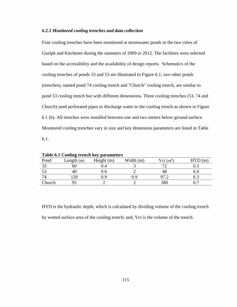
115
6.2.3 Monitored cooling trenches and data collection
Four cooling trenches have been monitored at stormwater ponds in the two cities of
Guelph and Kitchener during the summers of 2009 to 2012. The facilities were selected
based on the accessibility and the availability of design reports. Schematics of the
cooling trenches of ponds 33 and 53 are illustrated in Figure 6.1; two other ponds
(trenches), named pond 74 cooling trench and "Church" cooling trench, are similar to
pond 53 cooling trench but with different dimensions. Three cooling trenches (53, 74 and
Church) used perforated pipes to discharge water to the cooling trench as shown in Figure
6.1 (b). All trenches were installed between one and two meters below ground surface.
Monitored cooling trenches vary in size and key dimension parameters are listed in Table
6.1.
Table 6.1 Cooling trench key parameters
Pond Length (m) Height (m) Width (m) Vct (m³) HYD (m)
33 60 0.4 3 72 0.3
53 40 0.6 2 48 0.4
74 120 0.9 0.9 97.2 0.3
Church 95 2 2 380 0.7
HYD is the hydraulic depth, which is calculated by dividing volume of the cooling trench
by wetted surface area of the cooling trench; and, Vct is the volume of the trench.

116
Figure 6.1 (a) Pond 33 and (b) Pond 53, 74 and Church cooling trenches
schematics
Data were collected during summers, when the thermal warming of the stormwater
management ponds is highest. Tidbit temperature sensors were used to collect the water
temperature in cooling trenches (close to the cooling trench outlet) at ten-minute time
intervals. Pond water temperatures and water levels were collected using HOBO U20
water level loggers at the same time intervals. HOBO software was used to compensate
data and import data to Excel sheets for further analysis when necessary. Meteorological
data such as air temperature and precipitation were obtained from the Guelph Turf grass
Institute (GTI) Research Station and the GRCA weather innovation website.

117
The flows to the cooling trench are the pond outflows, which were generated using the
PCSWMM model to mimic the hydraulic conditions within the ponds. The pond water
level data, which were monitored during the course of the study, and used to calibrate the
PCSWMM model for ponds are shown as an example in Figure 6.2 for an event in pond
53.
Figure 6.2 PCSWMM model for pond water level time series versus observed pond
water level during an event start (Pond 53)
Event mean temperatures (EMT) for pond outlets and cooling trenches outlets were
calculated using equation (6.1), and named EMTO and EMTC respectively.
(6.1)
Q = the flow (m³/s)
Temp = the flow temperature (°C)

118
dt = the time increment of 10 minutes
n = the event duration (min)
A summary of collected and calculated data are listed in Table 6.2. The data were used to
develop an ANN model for prediction of the cooling effect of cooling trenches. The
cooling effect (Cooling) is the difference between the outlet event mean temperature and
cooling trench event mean temperature (EMTO – EMTC).
Table 6.2 Collected data and calculated EMTs
Note: MREST is the minimum residence time; it is calculated using volume of the cooling
trench and peak flow rate (Volume/Peak flow), also Cooling is the difference between
outlet event mean temperature (EMTO) and event mean temperature of cooling trench
(EMTC), PF stands for peak flow and CTinit is the initial temperature of water and rock
in cooling trench prior to rainfall. Vrunoff is the volume of runoff.
119
6.2.4 Cooling trench models
Current designs of studied cooling trenches in this research are based on steady-state
equations. The steady-state equations treat the cooling trench as a black box and calculate
the available heat transfer versus required heat transfer from between stored water and
rocks in the cooling trench followed by identification of the size of the cooling trench that
provides the necessary heat transfer to within the target temperature. In words, calculated
available heat transfer (for assumed cooling trench dimensions) will compare with
required heat transfer to get to the target temperature (e.g., how much heat should transfer
from pond water temperature of 32 ºC to the ground to get water temperature of 24 ºC at
the outlet of the cooling trench). If assumed size of the cooling trench is not provide the
required heat transfer then cooling trench will be resized to get to the required heat
transfer.
There are some transient equations and finite element equations which help to predict
water temperature in a cooling trench; however, all cooling trenches in this study,
designed by consultants, used steady-state methods to size the cooling trenches. One
objective of the current study is to compare the result of unsteady-state model or transient
model to calculate the cooling effect with the newly developed ANN model.
6.2.5 Unsteady (transient) state:
In an unsteady-state model of heat transfer, the rate of heat transfer varies with time due
to change in the internal energy of the system, and the temperature varies with time as
well as location. Most actual heat transfer processes, including heat transfer in cooling
trenches, are unsteady in nature. In unsteady-state cooling trench analysis, finite

120
difference equations can be used to calculate water and rock temperatures at differnt
locations and times. Two approaches of unsteady-state considered in this paper are:
1) In the approach of Herb et al. (2009), water and rock temperatures are calculated by
equations based on underground tanks. The water and rock temperature are calculated
for each time step based on the inflow and out flow rate:
(6.2)
is the volume of water in the crib
Heat transfer calculations are based on (i) the temperature of the water in the tank (Tw),
(ii) the average rock temperature in the tank (Tr) and (iii) the temperature of the
surrounding soil (Ts):
A finite difference equation for water temperature is:
(6.3)
Where:
is the surface area of rock in contact with water; is the contact area between the
rock and the crib wall; is the wetted area; is the heat transfer coefficient
for heat transfer to the rock; are the rock thermal conductivity and the rock

121
diameter respectively; is the heat transfer coefficient for heat
transfer to the soil; is the soil thermal conductivity; is the soil thermal diffusivity;
is the time scale for the thermal conduction in the soil; is the Rock volume.
The new rock temperature (Herb et al. 2009):
(6.4)
The cooling trenches are assumed to have no standing water between rainfall events.
Vw, Tw are volume and temperature of water; Ts, Tr, are temperature of soil and rock; Qin
and Tin are inflow rate and temperature.
2) Another approach (Thompson et al. 2008) based on laboratory experimental data,
calculates heat transfer between moving water in the crib and the cooler rocks influenced
by two factors: i) the convective transfer coefficient between water and the rocks and ii)
the thermal conductivity of the rocks.
Thompson et al. (2008) indicate that the convective transfer coefficient of turbulent water
flow through a typical rock crib could transfer heat at a rate approximately 20 times faster
than heat conduction into the rock. Therefore, the model assumes the heat transfer from
the water in the crib to the rock is limited by thermal conductivity of the rocks. Equations
(6.5) and (6.6) yield the water and rock temperature in the cooling trench as:

122
(6.5)
(6.6)
6.2.6 Development of an artificial neural network (ANN) model
Variables provided by a combination of monitoring, calculation, design maps and use of
hydrologic software (PCSWMM) as listed in Tables 6.1 and 6.2 are used to develop the
ANN model. List of input variables are:
1- Event mean temperature of pond’s outlet (EMTO, °C): EMTO is the event base
influent temperature to the cooling trench. This variable was necessarily to pick since the
main purpose of cooling trench is to reduce pond’s outlet temperature as much as
possible using design techniques; and, cooling efficiency of the cooling trench can
measure from water temperature difference between EMTO and EMTC.
2- Initial cooling trench temperature (CTinit, °C) which is the temperature of rock and
water in the trench prior to the rainfall events. From data analysis, it is observed that
larger differences between CTinit and EMTO provides more cooling effect and hence
utilization of CTinit as an essential variable.
3- Hydraulic depth of cooling trench (HYD, m): HYD is an important variable since it is
representative of contact area of water inside the trench with the trench's walls and the
heat will transfer from the walls to surround material.
4- Length of cooling trench (L, m): Length of cooling trench also influences the contact
time of influent water with water and rock inside cooling trench.

123
5- Minimum residence time (MREST): It is an important variable since the minimum
time for water to remain in trench will control by volume of water into trench and peak
flow (division of cooling trench volume by peak flow).
The mentioned variables were used as input parameters to develop the ANN model. The
desired output was the "COOLING" effect of the cooling trench. The ANN models then
were developed to predict the cooling effect of the rock cribs, the difference between
EMTO and EMTC. Figure 6.3 illustrates the developed network, which includes input
parameters, hidden layers, bias, and output of the model.
Size of rocks in a cooling trench is not likely an important parameter to use in cooling
trench modeling. Heat transfer calculations of the influence of the rock and water
revealed that less than 20% of the heat is absorbed by the rock in the rock cribs and the
bulk of the heat was dissipated from the bottom and sides of the rock crib to the soil and
water surrounding the crib as shown in Table 6.3. Therefore, rock diameter was not used
in the provided ANN model.

124
Table 6.3 Heat transfer calculation for observed events
Note: Constant values used in the calculation are: Porosity = 50%, Density (ρ) of water
and rock are assumed to be 998 and 2240 (kg/m³) respectively. Also, heat capacity (Cp)
for water and rock are 4180 and 200 (J/kg. ºK).

125
Figure 6.3 The ANN with its inputs, hidden layers, bias, and output
6.3 Result and Discussion
Two different cases were developed to analyze the cooling trench effectiveness. Case 1
inputs include design parameters as shown in Figure 6.3. The minimum residence time
(MREST), hydraulic depth (HYD), Length of trench (L) can be controlled by design
engineers, however, the other two parameters (cooling trench initial temperature of rock
and stored water temperature in the trench prior to event (CTinit) and event mean
temperature of the pond outlet (EMTO)) are beyond of the control of designers.
Conversely, in case 2 design parameters were excluded from input variables in order to
assess and identify the influence of design parameters on cooling effect as well as
variables’ contribution to the model. A list of inputs for both cases 1 and 2 and their level
of importance calculated by artificial neural network software (Tiberius) are shown in

126
Table 6.4. Once a model has been built, it is essential to determine which inputs are the
important ones. The model output was the cooling effect of the cooling trench
(COOLING) for both cases.
Table 6.4 Input parameters to develop ANN models to predict “COOLING”
Case 1
Variable Level of importance
Case 2
Variable Level of importance
EMTO 1.00 EMTO 1.0
CTinit 0.61 CTinit 0.6
HYD 0.23
L 0.03
MREST 0.03
Figure 6.4 illustrates the “COOLING” calculated by model versus observed “COOLING”
for both cases. R² for cases 1 and 2 are 0.92 and 0.82 respectively as shown in Figure 6.4.
As mentioned above, case 1 includes five parameters and case 2 excludes design
parameters (L, HYD, and MREST). Contribution of design parameters to increase R² is
therefore 10% and 82% of the variability of the predicted “COOLING” could explain by
remainder parameters (EMTO and CTinit).
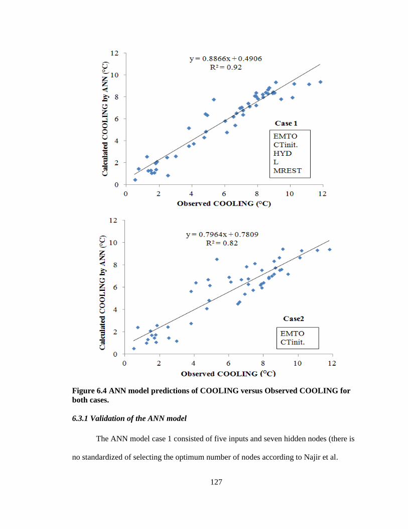
127
Figure 6.4 ANN model predictions of COOLING versus Observed COOLING for
both cases.
6.3.1 Validation of the ANN model
The ANN model case 1 consisted of five inputs and seven hidden nodes (there is
no standardized of selecting the optimum number of nodes according to Najir et al.

128
(1997). However, Caudill (1981), Fletcher and Goss (1993) claim that they obtained their
best results when to set an upper limit of hidden layer nodes between the number of
inputs and two times of the inputs number). In the current model, adding more hidden
layers did not improve the accuracy of the model so the seven hidden layer nodes were
kept. In order to find the overall trend, all data (53 data points for 4 cooling trenches)
were trained to create the predictive model for “COOLING.” In the second approach,
70% of data were randomly selected for training the network and the remainder was
chosen to test the model. The measures used to verify the model performance are listed
as: 1) R square; 2) the root- mean-square error (RMSE), which is frequently used to
measure the differences between values predicted by a model or an estimator and the
values actually observed. This measure compares only the different forecasting errors
within a dataset and not between different data sets, as it is scale-dependent. These
individual differences are also called residuals while RMSE serves to aggregate them into
a single measure of predictive power; 3) the coefficient of efficiency (CE) which is
recognized as a good alternative to R² (Nash and Sutcliffe, 1970) representing error
measure created by the differences in the observed and predicted means and variances; 4)
index of agreement (ID); 5) maximum absolute error (Max); 6) mean absolute error
(MAE); 7) mean absolute percentage error (MAPE).The measure of MAPE also known
as mean absolute percentage deviation. It is a measure of accuracy of a method for
constructing fitted time series values in statistics, specifically in trend estimation. It
usually expresses accuracy as a percentage, and. The above-mentioned measures were
calculated for each data set to describe the predictive capability of the model. Table 6.5

129
illustrates the coefficient and different statistical measures for model evaluation and their
range of variability.
Table 6.5 Coefficient and different statistical measures for model evaluation and
their range of variability
Coefficient or Measure Equation∗ Range of
Variability
Coefficient of
Determination
0 to 1
Root Mean Square Error RMSE=
0 to ∞
Coefficient of Efficiency
Nash and Sutcliffe(1970) Esn=1-
-∞ to 1
Index of Agreement
Willmout(1984) ID=1-
0 to 1
Max Absolute Error Max = 0 to ∞
Mean absolute error
0 to ∞
Mean absolute percentage
error
0 to ∞
Note: Oi and pi, are observed and predicted values respectively
Statistical performances are summarized in Table 6.6, for the trained and tested newly
developed predictive "Cooling" model. Statistical performances of both cases show the
acceptable accuracy for newly developed models.

130
Table 6.6 Statistical performances of “COOLING” model for Train and Test values
(CASE 1: 5 input parameters and Case 2: 2 input parameters as shown in Table 6.3)
Statistical
Term†
Overall
Case 1 Case2
70%Train
Case 1 Case2
30%Test
Case 1 Case2
RMSE 1.01 1.42 0.77 1.27 1.14 1.61
SMRE 0.50 0.93 0.36 0.91 0.92 1.01
MAX 3.44 3.93 2.50 3.49 3.45 4.07
MAE 0.68 1.14 0.49 1.05 1.01 1.23
MAPE 16.87 25.13 12.77 23.38 19.34 27.71
E 0.92 0.83 0.94 0.89 0.91 0.80
ID 0.95 0.86 0.98 0.90 0.96 0.84
R² 0.92 0.82 0.93 0.81 0.89 0.83 If all predicted and observed values were the same, then the statistics would yield: MAX=0.0, MAE=0.0,
MAPE=0.0, RMSE=0.0, R²=1, E=1, and ID=1. RMSE is root mean square error, SMRE square of the
mean root error, MAX is maximum absolute error, MAE maximum absolute error, MAPE mean absolute
percentage error and E coefficient of efficiency, ID index of agreement, and R² coefficient of
determination.
6.3.2 Sensitivity analysis of the variables of ANN model
A sensitivity analysis was employed in order to identify which variable has more
influence on "COOLING". Therefore, the variables in the developed ANN model (case 1)
were perturbed by adding 10%. The marginal sensitivity coefficient was determined by
Equation (6.8):
(6.8)
Where Sc is the marginal sensitivity coefficient of the equation, is the change in the
calculated objective function, and is the change in the parameter. Normalizing the
parameters indicates the percent change in the objective function for a 1% change in each

131
individual parameter. The marginal sensitivity coefficients were normalized to establish
a basis of comparison using Equation (6.9):
∗
(6.9)
Where is the normalized sensitivity coefficient, is the expected value of the
perturbed parameter, and is the expected solution. Table 6.7 illustrates the sensitivity
and effect of the input parameters on the "Cooling" for the developed ANN model.
Table 6.7 Sensitivity analysis results
Perturbed †
Variable L EMTO HYD CTinit
MREST COOLING Sc Sn
Base 80 20.85 0.49 14.13 5.69 6.32
L 88
6.74 0.05 0.68
EMTO
22.94
9.18 1.37 3.43
HYD
0.54
6.74 8.40 0.67
CTinit
15.54 5.51 -.057 -1.62
MREST
6.26 7.07 1.32 1.17
† :Note: L length of trench, EMTO event mean temperature of outlet, HYD hydraulic depth, CTinit initial
temperature of cooling trench, MREST minimum resident time, COOLING is cooling effect of cooling
trench (EMTO - EMTC), Sc sensitivity coefficient, Sn normalized sensitivity coefficient.
From these results, the model is determined as most sensitive to change in event mean
temperature of ponds’ outlet (EMTO) or influent temperature to the cooling trench due to
the absolute value of Sn belong to EMTO is the greatest. The next levels of importance
belong to initial temperature of rock and water in the cooling trench, minimum residence
time, length of cooling trench, and hydraulic depth of trench respectively.

132
Figure 6.5 The sensitivity analysis results of the ANN model
for CTinit, EMTO, L, HYD, and MREST
Figure 6.5 presents the sensitivity analyses of the trained ANN model; these analyses
reveal that:
1- Reducing the hydraulic depth in the model from 0.8 to 0.3 m results in a 2 ºC
improvement in the stormwater runoff cooling trench efficiency of the trench.

133
This better cooling efficiency indicated by the model, can be explained physically
since reducing the hydraulic depth for a constant volume will lead to a longer
and/or wider trench providing more surface area for heat transfer to the
surrounding, cooler, environment.
2- Increasing the length of the cooling trench from 50 to 100 m, in the model, results
in more than 3 °C improvement in the stormwater runoff cooling efficiency of the
trench as indicated by the model. As above, this is physically possible since
increasing the length can provide more contact area for heat transfer.
3- Increasing minimum residence time from 1 to 6 hours in the model resulted in a
2 °C improvement in the stormwater runoff cooling effect. Physically, this is
explained by the longer the time for heat transfer the greater the cooling effect.
4- Increasing the EMTO in the model (which results in larger difference between
CTinit and EMTO since CTinit is kept constant in the sensitivity analyses) results
in an improved cooling effect in a 1 to 1 correspondence. This is consistent with
the observed data in Figure 6.7, which shows a 0.9 °C improvement in cooling for
every 1 °C increase in EMTO.
5- The cooling trench initial temperature analysis shows that reducing CTinit by
1 °C results in an almost 1 °C improvement in the cooling effect of the trench.
The predictive capability of the ANN model as opposed to existing physical base
unsteady-state model (introduced in section 6.2.5) is illustrated in Figure 6.6.

134
Figure 6.6 A comparison between the Cooling calculated by ANN versus unsteady
model.
The ANN model shows a good predictive ability to determine the cooling effect of the
cooling trench. The ANN model explains 92% of variability of the cooling effect; as
opposed to cooling effect predicted by unsteady-state model that explains 47% of
variability of the cooling effect for the current data set as shown in Figure 6.6. It is
noticeable that no water assumed to be stored between events in cooling trench in the
present unsteady-state model, which could be the main reason for smaller correlation.
A regression model using observed data revealed that there is a good correlation between
differences of EMTO and CTinit (EMTO – CTinit) and observed COOLING, as shown
in Figure 6.7. This confirms the cooling effect most likely to happen when the difference
between EMTO and CTinit is larger. In words, more cooling occurs when the difference
between temperature of water entering into the cooling trench and temperature of rock

135
and water in the trench prior to the event is larger. The regression model was able to
explain 80% of variability in the COOLING.
Figure 6.7 The difference between EMTO and CTinit Versus COOLING
6.4 Conclusions
The ANN model, trained using three summers of cooling trench data, was able to explain
92% of the variability in the cooling effect of four studied cooling trenches in the Cities
of Guelph and Kitchener. The results show that the cooling effects of the cooling trenches
were significantly influenced by influent water temperature (or event mean temperature
of the pond’s outlet to the cooling trench) and the initial temperature of stored water and
rock in the cooling trench. The difference between EMTO and initial rock and water
temperature in a cooling trench has a large influence on cooling effect and their

136
correlation estimate to be of R² = 0.80; this confirms the importance of the differences
between EMTO and CTinit on cooling trench performance.
Heat transfer calculations of the influence of the rock and water revealed that less than
20% of the heat is absorbed by the rock in the rock cribs and the bulk of the heat was
dissipated from the bottom and sides of the rock crib to the soil and water surrounding the
crib.
Sensitivity analyses of the developed ANN model revealed that length (L) and hydraulic
depth of trench (HYD) are the key design parameters that influence the cooling efficiency
of a trench. Reducing the hydraulic depth from 0.8 to 0.3 m resulted in a 2 °C
improvement in the stormwater runoff cooling efficiency of the trench as indicated by the
model. Increasing length of the trench from 50 to 100 m in the model results in a 3 °C
improvement in the stormwater runoff cooling efficiency of the trench; and increasing
minimum residence time from 1 to 6 hours in the model results in a 2 °C improvement in
the stormwater runoff cooling efficiency of the trench. Therefore, it is important to
promote optimum design of cooling trenches with shallower HYD, longer length, and
longer residence time.

137
6.5 References
Armour, C.L., 1991. Guidance for evaluating and recommending temperature regimes to
protect fish, US Dept. of the Interior, Fish and Wildlife Service.
Arrington, K., 2009. Mapping infiltration rates in Dane County, Wisconsin, 132.
Booth, D.B., Bledsoe, B.P., 2009. Streams and urbanization, the water environment of
cities. USA, Springer, pp. 93-123.
Brabec, E., 2002. Impervious surfaces and water quality: a review of current literature
and its implications for watershed planning. Journal of Planning Literature, 16(4), 499-
514
Brierley, P., 2007. Neural Network Software (Tiberius v5.5.0).
http://www.philbrierley.com/phil.html
Brun, S. and L. Band. 2000. Simulating runoff behavior in an urbanizing watershed.
Computers, Environment and Urban Systems, 24(1), 5-22
Cairns, J., 1971. Thermal pollution: a cause for concern. Journal of Water Pollution
Control Federation. 43(1), 55-66.
Chen, Y., Chang, F.J., 2009. Evolutionary artificial neural networks for hydrological
systems forecasting. Journal of Hydrology. 367, 125-137.
Eaton, J., J. McCormick, B. Goodno, D. O'brien, H. Stefany, M. Hondzo, et al. 1995. A
field information-based system for estimating fish temperature tolerances. Fisheries,
20(4), 10-18
Herb, W.R., Mohseni, O., Stefan, H.G., 2009. Simulation of temperature mitigation by a
stormwater detention pond. Journal of the American Water Resources Associate. 45,
1164-1178.

138
James, W., Verspagen, B., 1997. Thermal enrichment of stormwater by urban pavement.
Advances in Modeling the Management of Stormwater Impacts CHI, Guelph, Canada. 5,
155-177.
Kieser, M.S., Fang, A.F., Spoelstra, J.A., 2003. Role of urban stormwater best
management practices in temperature TMDLs. Proceedings of the Water Environment
Federation. 2003, 1716-1739.
Kumar, B., 2012. Neural network prediction of bed material load transport. Hydrological
Sciences Journal. 57, 956-966.
Lyons, J., L. Wang, and T. D. Simonson. 1996. Development and validation of an index
of biotic integrity for coldwater streams in Wisconsin. North American Journal of
Fisheries Management, 16(2), 241-256.
Nash, J. E. and J. V. Sutcliffe (1970), River flow forecasting through conceptual models
part I — A discussion of principle, Journal of Hydrology. 10 (3), 282–290.
Nelson, K. C. and M. A. Palmer. 2007. Stream temperature surges under urbanization and
climate change: data, models, and responses. Journal of the American Water Resources
Association, 43(2), 440-452.
Poole, K., 2009. Investigation of storm water management professionals' perceptions of
permeable interlocking concrete pavers as a stormwater management option, 136.
Rafiq, M., Bugmann, G., Easterbrook, D., 2001. Neural network design for engineering
applications. Computer and Structures. 79, 1541-1552.
Roa-Espinosa, A., Wilson, T., Norman, J., Johnson, K., 2003. Predicting the impact of
urban development on stream temperature using a Thermal Urban Runoff Model
(TURM).Modeling the effect of the natural environment and urban runoff on stream
temperature, 369-389

139
Sahoo, G., Schladow, S., Reuter, J., 2009. Forecasting stream water temperature using
regression analysis, artificial neural network, and chaotic non-linear dynamic models.
Journal of Hydrology. 378, 325-342.
Schueler, T.R., Galli, J., 1994. Environmental impacts of stormwater ponds. Watershed
Protection Techniques 1(3) 100-111.
Shaver, E., J. Maxted, G. Curtis, and D. Carter. 1995. Watershed protection using an
integrated approach., 435-459.
Shigidi, A., Garcia, L.A., 2003. Parameter estimation in groundwater hydrology using
artificial neural networks. Journal of Computing in Civil Engineering. 17, 281-289.
Tayfur, G., Singh, V.P., 2005. Predicting longitudinal dispersion coefficient in natural
streams by artificial neural network. Journal of Hydraulic Engineering. 131, 991-1000.
Thompson, A.M., Wilson, T., Norman, J., Gemechu, A., Roa‐Espinosa, A., 2008.
Modeling the effect of summertime heating on urban runoff temperature1. Journal of the
American Water Resources Association. 44, 1548-1563.
Thompson, A. M., Vandermuss, A. J., Norman, J. M., Roa-Espinosa, A., 2008. Modeling
the effect of a rock crib on reducing stromwater runoff temperature. Journal of the
American Society of Agriculture and Biological Engineers. 51(3), 947- 960.
Tokar, A.S., Johnson, P.A., 1999. Rainfall-runoff modeling using artificial neural
networks. Journal of Hydrology. 4, 232-239.
Walker, D., 1998. Modelling residence time in stormwater ponds. Ecological
Engineering. 10, 247-262.
Wang, G., Chen, S., Barber, M., Yonge, D., 2004. Modeling flow and pollutant removal
of wet Detention Pond Treating Stormwater Runoff. Journal of Environmental
Engineering. 130, 1315-1321.

140
Willmott C., 1984. On the evaluation of model performance in physical geography. In
Spatial Statistical and Models, Boston; 443-460.
Wu, C., Chau, K., 2011. Rainfall–runoff modeling using artificial neural network coupled
with singular spectrum analysis. Journal of Hydrology. 399, 394-409.
Zaghloul, N., Kiefa, A., 2001. Neural network solution of inverse parameters used in the
sensitivity-calibration analyses of the SWMM model simulations. Advances in
Engineering Software. 32, 587-595.

141
Chapter 7
Conclusions and Recommendations for Future Research

142
7.1 Research Summary
The use of stormwater ponds to control runoff and peak flow in urbanized areas has
significantly increased in recent decades due to changes in legislation (e.g., Conservation
Authorities and Ministry of Environment guidelines). They are a popular design approach
and can be effective at reducing peak flows, reducing the concentration of total
suspended solids (TSS) and associated contaminants from urban and industrial surface
runoff during storm events. However, ponds can have negative thermal effects on aquatic
habitat. Thermal pollution from urban runoff is a significant contributor to the
degradation of cold-water ecosystems, as water temperature is one of the most important
factors influencing the distribution of aquatic organisms. Increasing the water
temperature or thermal enrichment of a creek or pond can disrupt the aquatic ecosystem
due to thermal shocks to receiving streams, and could be lethal for fish such as trout. In
order to develop better management practices to protect aquatic habitats, there is a great
need for improved understanding of thermal enrichment of urban stormwater
management ponds.
This study reduced the knowledge gap that currently exists concerning thermal
enrichment of stormwater management ponds. The following objectives were defined to
achieve a better understanding of the effects of stormwater management ponds on aquatic
ecosystem temperature in summer conditions:
i) Determine the thermal impact of urbanization on stormwater management ponds
inlet water temperature during rainfall events,
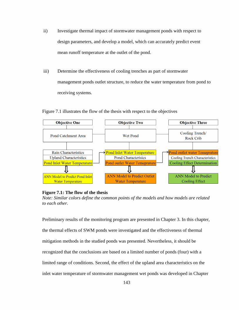
143
ii) Investigate thermal impact of stormwater management ponds with respect to
design parameters, and develop a model, which can accurately predict event
mean runoff temperature at the outlet of the pond.
iii) Determine the effectiveness of cooling trenches as part of stormwater
management ponds outlet structure, to reduce the water temperature from pond to
receiving systems.
Figure 7.1 illustrates the flow of the thesis with respect to the objectives
Figure 7.1: The flow of the thesis
Note: Similar colors define the common points of the models and how models are related
to each other.
Preliminary results of the monitoring program are presented in Chapter 3. In this chapter,
the thermal effects of SWM ponds were investigated and the effectiveness of thermal
mitigation methods in the studied ponds was presented. Nevertheless, it should be
recognized that the conclusions are based on a limited number of ponds (four) with a
limited range of conditions. Second, the effect of the upland area characteristics on the
inlet water temperature of stormwater management wet ponds was developed in Chapter

144
4. The provided Artificial Neural Network (ANN) model is applicable for practitioners to
predict the runoff temperature at the inlet of the stormwater ponds, making use of the
same variables used to build the predictive ANN model. The model is event based and
provides the event mean temperature of the runoff for any event of interest. However, the
conclusions based on the presented ANN model is limited by the number of catchments
studied (four). This chapter has been published in the Journal of Hydrology.
Third, an artificial neural network has been trained to predict event mean temperatures at
the pond outlet. The model was then used to find the sensitivity of variables in the model
on water temperature at the pond outlet. The ANN model provides a good level of
accuracy in predicting the event mean temperatures at the pond outlet. The provided
model has potential for practical use, and the combination of the two developed models
(predict event mean temperatures at the inlet and outlet), can predict thermal enrichment
of a stormwater pond. However, limitations related to the models include the limited
range of parameters used such as pond volume, and average depth of the ponds. In
addition, ponds were constructed according to the Ontario guidelines, which may not be
consistent with design approaches in other jurisdictions and this may affect the
applicability of the models to alternative design approaches. This chapter has been
submitted to the Journal of Hydrology.
In Chapter 6, an evaluation of the performance of the cooling trench/rock crib after the
stormwater management ponds is presented. To accomplish this, the monitoring results,
along with the developed artificial neural network model, were used to advance the
understanding of key design parameters, which influence the performance of rock cribs

145
or cooling trenches. A potential practical use of the developed ANN model is to predict
and estimate the cooling effect of a cooling trench prior to construction.
7.2 Conclusions
This research will contribute for evaluation of thermal contribution of stormwater
management ponds, aiding in minimizing the negative environmental effects of ponds by
providing means and design variables in a modeling outlook. This chapter summarizes
the conclusions from each of the previous chapters to provide a set of cohesive
conclusions. This information can lead to improve engineering design guidelines for
urban stormwater management systems discharging to temperature sensitive receiving
streams.
Objective one
Artificial neural networks have shown a great ability in modeling complex
environmental systems with both linear and nonlinear relations. However, the novelty of
the current study is using ANN models to investigate thermal enrichment of urbanized
areas from upland to receiving water bodies. The research begins with upland area or
pond watershed characteristics and their influence on runoff temperature. The most
significant variable was found to be the event mean temperature of rainfall, which
explains about 70% in the variability of event mean temperatures of runoff to stormwater
ponds. A uniqueness of the study is using two key input variables which are sewer pipe
length and storm sewer pipe network density in developed model for runoff temperature
at the pond inlet. Both variables have been found to have a pronounced effect on the

146
cooling of runoff; thus, they should be considered in the design of stormwater
management systems when temperature effects are important. For example, the
sensitivity analyses using the ANN model shows that when longest sewer pipe length is
increased from 370 to 970 m, runoff temperature at the catchment outlet dropped by 2.5
°C. Therefore, the cooling effect of the sewer pipe system can compensate for the
warming effect of the asphalt and concrete paved surfaces of the catchment area. This
result suggests that it would be more beneficial to promote the design of a network of
smaller distributed stormwater management facilities that directly discharge to the outlet
with underground pipes - rather than the more popular preference of municipalities to use
few but large facilities located near the receiving watercourse.
Furthermore, the next levels of importance belong to impervious percentage, asphalt
temperature and rainfall characteristics such as maximum rainfall intensity, rainfall
duration and magnitude. A remarkable point with respect to imperviousness of upland
area is that every 10% increase in impervious percentage increased the runoff
temperature to the pond by 1 °C. The sensitivity analyses of the developed model confirm
that limiting the percent impervious cover or maximizing green areas in the catchment
area when possible is a preferable practice.
Objective two
The effect of pond design parameters on stormwater runoff temperature and mitigation
features, such as bottom-draw outlet, were investigated. Measurements from stormwater
management ponds demonstrate that avoiding the design of very shallow ponds (less than

147
0.5 m), and keeping average depth greater than 1.2 m, can result in significant decrease in
outlet event mean temperature. It is likely that deeper bottom- draw outlet structures
provide more cooling effects at the outlet of the system. However, limited additional
cooling was observed below a depth of 1.2 m, as most temperature decreases happened
between the top and 1.2 m below the surface.
An artificial neural network model was trained to predict the event mean temperature at
the pond outlet (EMTO) using collected monitoring data. The provided model explains
99% of the variability in event mean temperatures at the pond outlet. Sensitivity analyses
show that increasing permanent pond volume from 2000 to 4000 m³ - while keeping all
other parameters constant - results in an average increase of 5 °C in EMTO. Therefore,
ponds with larger permanent pool volumes will tend to release the warmer water sitting in
the ponds. As a result, less thermal interaction with the fresh event runoff at the pond
inlet was observed. It can physically be explained since larger ponds (for a constant
depth) have greater surface areas and thus absorbed more solar energy than smaller ponds
with similar depths.
Similarly , sensitivty analysis using ANN model for travel path ratio reveals that
increasing travel path ratio using baffles results in increasing event mean temperature at
the pond outlet. For instance, increasing travel path ratio from 0.6 to 1.2 m leads to an
average increase of 6 °C in event mean temperature at the pond outlet. A possible reason
is that the larger travel path ratio can lead to less mixing of the water that is sitting in the
pond with the cooler fresh event runoff.

148
Hence, larger volume ponds and ponds with elongated travel path tend to discharge more
of the warmer water that is sitting in the pond than the cooler, fresh event runoff.
However, the increasing average pond depth from 0.6 to 1.0 m, in the model, results in,
up to 9 °C decreases in EMTO; therefore, design of ponds with average depths greater
than 1.2 m can result in significant decreases in EMTO.
The results can lead to the promotion of the design of deeper ponds with bottom-draw
outlet and smaller travel path ratio (TPR). However, the implications of this approach on
other performance criteria besides effluent temperature should be evaluated.
Objective three
Monitoring results along with developed artificial neural network model were employed
to advance the understanding of key design parameters that influence the cooling effect
of rock cribs after the ponds. The sensitivity analyses of the developed model revealed
that the cooling effects of the trenches were influenced mostly by the initial temperature
of water and rock in the cooling trench. The influent temperature or event mean
temperature of the pond’s outlet to the trench also influenced the cooling effect, but to a
lesser degree. Heat transfer calculations of the influence of the rock and water revealed
that less than 20% of the heat is absorbed by the rock in the rock cribs and the bulk of the
heat was dissipated from the bottom and sides of the rock crib to the soil and water
surrounding the crib.
Sensitivity analyses of the developed ANN model revealed that the length (L) and
hydraulic depth of trench (HYD) are the key design parameters that influence the cooling
efficiency of the trench. Reducing the hydraulic depth from 0.8 to 0.3 m, in the model,

149
results in a 2 °C improvement in the stormwater runoff cooling efficiency of the trench.
Increasing the length of the trench from 50 to 100 m, in the model, results in a 3 °C
improvement in the stormwater runoff cooling efficiency of the trench. Finally,
increasing the minimum residence time from 1 to 6 hours results in a 2 °C improvement
in the stormwater runoff cooling efficiency of the trench. Therefore, it is important to
promote cooling trenches with shallower hydraulic depths, longer lengths, and longer
residence times to maximize their performance.
7.3 Recommendations for Future Research
Research on urban hydrology and water quality, especially related to thermal enrichment
of the receiving systems deserves more attention from researchers to improve the current
dearth of literature. With the observation made during this research, the following
recommendations are made for future research:
i) An important subject for future research could be an investigation of thermal
contribution of stormwater management ponds on thermal enhancement of
streams. It is necessary to study thermal load into streams by constructed ponds.
One example question is how much thermal load a stream can tolerate for the sake
of fisheries with respect to ponds and development.
ii) Including variables such as base temperature, time series input of runoff
temperature in the US EPA SWMM would greatly develop its capabilities to
simulate thermal aspect of urban water quality and runoff temperatures discharge
to receiving systems. Once the thermal aspects of US EPA SWMM model have

150
been enhanced, different drainage areas can be modeled to simulate various
scenarios related to thermal impact of end of pipe control. Also, the model can be
used to evaluate existing and novel best management practices including
stormwater management ponds.
iii) Continuous monitoring of different zones including upland area, pond, outlet and
receiving systems or streams should be undertaken to collect more data on runoff
water temperature to the catchment and water temperature into sewer pipes, pond
and their outlet, and finally to water bodies. This will provide the opportunity to
develop a comprehensive model on thermal impact of urbanization.
iv) Concerning cooling trench of stormwater management ponds, continuous
monitoring of water temperature discharge to and out of the cooling trench and
some extra points inside the cooling trench would be a great help to create
accurate predictive models. It is highly recommended that both pond water level
and cooling trench water level be monitored to investigate the initial conditions
prior to storm events. Furthermore, an installed rain gauge to collect the rainfall
data in site will provide the opportunity to improve the accuracy of the modeling.
v) In addition, there is potential in studying the influence of pond orientation and
shape on the thermal enrichment. An example question is how is the thermal
effect of elongated and narrower pond shape as oppose to wider pond.

151
vi) Finally, future study in the thermal impact of stormwater ponds on groundwater
quality (negative/positive) is necessary.
152
References
Ackerman, D., Stein, E., 2008. Evaluating the Effectiveness of Best Management
Practices Using Dynamic Modeling. Journal of Environment Engineering. 134, 628-639.
Agersborg, H., 1930. The influence of temperature on fish. Ecology. 11, 136-144.
Arrington, K., 2009. Mapping infiltration rates in Dane County, Wisconsin., 132.
Anderson, B., Watt, W., Marsalek, J., 2002. Critical issues for stormwater ponds:
Learning from a decade of research. Diffuse/Non-point Pollution and Watersheds
Management. 45, 277-283.
Asaeda, T., Ca, V.T., Wake, A., 1996. Heat storage of pavement and its effect on the
lower atmosphere. Atmos.Environ. 30, 413-427.
Billstein, M., Svensson, U., Johansson, N., 1999. Development and Validation of a
Numerical Model of Flow Through Embankment Dams–Comparisons with Experimental
Data and Analytical Solutions. Transp.Porous Media. 35, 395-406.
Bogan, T., Mohseni, O., Stefan, H.G., 2003. Stream temperature-equilibrium temperature
relationship. Water Resources Research. 39, 7.1-7.12.
Bogan, T., Stefan, H.G., Mohseni, O., 2004. Imprints of secondary heat sources on the
stream temperature/equilibrium temperature relationship. Water Resources Research. 40,
W12510.
Boulton , 2008. Stream ecology. Online water encyclopedia:
http://www.waterencyclopedia.com/Re-St/Stream-Ecology-Temperature-Impacts-on.html
Booth, D.B., Bledsoe, B.P., 2009. Streams and urbanization, the water environment of
cities. USA, Springer, pp. 93-123.

153
Bowden, G.J., Dandy, G.C., Maier, H.R., 2005. Input determination for neural network
models in water resources applications. Part 1—background and methodology. Journal of
Hydrology. 301, 75-92.
Brabec, E., 2002. Impervious surfaces and water quality: a review of current literature
and its implications for watershed planning. Journal of Planning Literature. 16, 499-514.
Bravo, H.R., Feng, J., Hunt, R.J., 2002. Using groundwater temperature data to constrain
parameter estimation in a groundwater flow model of a wetland system. Water Resources
Research 38, 1153.
Brett, J., 1956. Some principles in the thermal requirements of fishes. The Quarterly
Review of Biology. 31, 75-87.
Brun, S., Band, L., 2000. Simulating runoff behavior in an urbanizing watershed.
Computing , EnvironmentalUrban Systems. 24, 5-22.
Cairns, J., 1971. Thermal pollution: a cause for concern. Journal of Water Pollution
Control Federation. 43(1), 55-66.
Carleton, J.N., Grizzard, T.J., Godrej, A.N., Post, H.E., 2001. Factors affecting the
performance of stormwater treatment wetlands. Water Resources Research. 35, 1552-
1562.
Cathcart, T.P., Wheaton, F.W., 1987. Modeling temperature distribution in freshwater
ponds. Aquaculture Engineering. 6, 237-257.
Chen, Y., Chang, F.J., 2009. Evolutionary artificial neural networks for hydrological
systems forecasting. Journal of Hydrology. 367, 125-137.
Cherry, D., Dickson, K.L.J., Stauffer, J., 1977. Preferred, avoided, and lethal
temperatures of fish during rising temperature conditions. Journal of the Fisheries
Research Board of Canada. 34, 239-246.

154
Creaser, C.W., 1930. Relative importance of hydrogen-ion concentration, temperature,
dissolved oxygen, and carbon-dioxide tension, on habitat selection by brook-trout.
Ecology., 246-262.
Coutant, C.C., 1970. Compilation of temperature preference data. Journal of Fish
Research Canada. 34, 740 - 745.
Credit Valley Conservation. 1996. Stormwater Management Guidelines.
Credit Valley Conservation. 2012. Thermal impact of urbanization.
Davidson, B., Bradshaw, R., 1967. Thermal pollution of water systems. Environmental
Science Technology. 1, 618-630.
Design spesification and requirements mannual, London, Ontario 2010.
Dingman, S.L., 1972. Equilibrium temperatures of water surfaces as related to air
temperature and solar radiation. Water Resources Research 8, 42-49.
Dodds, W.K., 2002. Freshwater ecology concepts and environmental application. San
Diego, CA: Academic Press.
Eaton, J., McCormick, J., Goodno, B., O'brien, D., Stefany, H., Hondzo, M., et al., 1995.
A field information-based system for estimating fish temperature tolerances. Fisheries.
20, 10-18.
Fang, X., Stefan, H.G., 1996. Dynamics of heat exchange between sediment and water.
Water Resources Research .32, 1719-1727.
Fennessey, L.A.J., Hamlett, J.M., Aron, G., LaSota, D., 2001. Changes in Runoff Due to
Stormwater Management Pond Regulations. J.Hydrol.Eng. 6, 317.
Frank, R., Davey, N., Hunt, S., 2001. Time series prediction and neural networks. Journal
of Intelligent and Robotic Systems. 31, 91-103.

155
Fry, F.E.J. 1967. Responses of vertebrate poikilotherms to temperature. Academic Press,
New York.
Galli, J., 1991. Thermal impacts associated with urbanization and stormwater
management best management practices. Metropolitan Washington Council of
Governments, Maryland Department of Environment, Washington, DC.
Galli, J., Maryland. Sediment and Stormwater Administration, Metropolitan Washington
Council of Governments. Department of Environmental Programs, 1990. Thermal
impacts associated with urbanization and stormwater management best management
practices, Department of Environmental Programs, Metropolitan Washington Council of
Governments.
Gao, J., Merrick, N.P., 1996. Simulation of temperature and salinity in a fully mixed
pond. Environ.Software. 11, 173-178.
Ghosh-Choudhury, T., Mandal, C.C., Woodruff, K., St Clair, P., Fernandes, G.,
Choudhury, G.G., et al., 2009. Fish oil targets PTEN to regulate NFκB for
downregulation of anti-apoptotic genes in breast tumor growth. Breast Cancer Res.Treat.
118, 213-228.
Ham, J., Toran, L., Cruz, J., 2006. Effect of upstream ponds on stream temperature.
Environment Geology. 50, 55-61.
Herb, W.R., Janke, B., Mohseni, O., Stefan, H.G., St Paul, M., 2007. Estimation of
Runoff Temperatures and Heat Export from Different Land and Water Surfaces.
Herb, W.R., Janke, B., Mohseni, O., Stefan, H.G.., 2008. Thermal pollution of streams by
runoff from paved surfaces. Hydrology Processes. 22, 987-999.
Herb, W.R., Mohseni, O., Stefan, H.G., 2009. Simulation of temperature mitigation by a
stormwater detention pond. Journal of American Water Resources Associate. 45, 1164-
1178.
156
Hossain, M., Alam, M., Yonge, D.R., Dutta, P., 2005. Efficiency and Flow Regime of a
Highway Stormwater Detention Pond in Washington, USA. Water, Air, Soil Pollution.
164, 79-89.
Jain, S., Das, A., Srivastava, D., 1999. Application of ANN for reservoir inflow
prediction and operation. Journal of Water Resources Planning and Management. 125,
263-271.
James, W., Verspagen, B., 1997. Thermal enrichment of stormwater by urban pavement.
Advances in Modeling the Management of Stormwater Impacts. 5, 155-177.
Janke, B.D., Herb, W.R., Mohseni, O., Stefan, H.G., 2009. Simulation of heat export by
rainfall-runoff from a paved surface. Journal of Hydrology. 365, 195-212.
Jha, G.K., 2007. Artificial neural networks and its applications.
http://www.iasri.res.in/ebook/EBADAT/5
Jia, Y., Ni, G., Kawahara, Y., Suetsugi, T., 2001. Development of WEP model and its
application to an urban watershed. Hydrology Processes. 15, 2175-2194.
Jones, M.P. 2008. Effect of urban stormwater BMPs on runoff temperature in trout
sensitive regions. Ph.D. Dissertation. North Carolina State University.
Jones, M.P., and Hunt, W.F., 2007. Stormwater BMPs for trout waters. North Carolina
Cooperative Extension Service. Online: www.bae.ncsu.edu/stormwater/PulicationFiles.
Kehl, O., Wichern, M., Lübken, M., Horn, H., 2009. Analysis of design approaches for
stabilization ponds under different boundary conditions—A comparison. Ecology
Engineering. 35, 1117-1128.
Kieser, M.S., Fang, A.F., Spoelstra, J.A., 2003. Role of urban stormwater best
management practices in temperature TMDLs. Proceedings of the Water Environment
Federation. 2003, 1716-1739.

157
Kinouchi, T., Yagi, H., Miyamoto, M., 2007. Increase in stream temperature related to
anthropogenic heat input from urban wastewater. Journal of Hydrology. 335, 78-88.
Klemetson, S.L., Rogers, G.L., 1985. Aquaculture pond temperature modeling.
Aquaculture Engineering. 4, 191-208.
Kumar, B., 2012. Neural network prediction of bed material load transport. Hydrological
Sciences Journal. 57, 956-966.
Lamourex, J., Tiersch, T.R., Hall, S.G., 2006. Sensitivity analysis of the pond heating and
temperature regulation (PHTAR) model. Aquaculture Engineering. 34(2), 117-130.
Larm, T., 2000. Stormwater quantity and quality in a multiple pond-wetland system:
Flemingsbergsviken case study. Ecology Engineering. 15, 57-75.
LeBlanc, R.T., Brown, R.D., FitzGibbon, J.E., 1997. Modeling the effects of land use
change on the water temperature in unregulated urban streams. Journal of Environmnet
Management. 49, 445-469.
Li, Y., and James, W. 2004. Thermal enrichment by stormwater. CHI monograph 12.
651-664.
Lieb, D.A., Carline, R.F., 2000. Effects of urban runoff from a detention pond on water
quality, temperature and caged Gammarus minus (Say)(Amphipoda) in a headwater
stream. Hydrobiologia. 441, 107-116.
Lieb, D., Carline, R., 2000. BIOLOGY: The Effects of Urban Runoff from a Detention
Pond on the Macroinvertebrate Community of a Headwater Stream in Central
Pennsylvania. Journal of Pennsylvania Academy of Science. 73, 99-105.
Losordo, T.M., Piedrahita, R.H., 1991. Modelling temperature variation and thermal
stratification in shallow aquaculture ponds. Ecology Modeling. 54, 189-226.

158
Lyons, J., Wang, L., Simonson, T.D., 1996. Development and validation of an index of
biotic integrity for coldwater streams in Wisconsin. N.Am.J.Fish.Manage. 16, 241-256.
Marsalek, J., Rochfort, Q., Grapentine, L., Brownlee, B., 2002. Assessment of
stormwater impacts on an urban stream with a detention pond. Water Science and
Technology. 45, 255-264.
Marshall Macklin Monaghan (MMM) Limited and LGL Limited. 1993. Hanlon Creek
Watershed Plan Draft Final Report. April 1993.
Ministry of the Environment (MOE). 2003. Stormwater Management and Design
Manual. March 2003.
Ministry of the Environment (MOE). 1994. Stormwater Management and Design
Manual.
Mohseni, O., Stefan, H.G., 1999. Stream temperature/air temperature relationship: a
physical interpretation. Journal of Hydrology. 218, 128-141.
Mohseni, O., Stefan, H.G., Erickson, T.R., 1998. A nonlinear regression model for
weekly stream temperatures. Water Resour.Res. 34, 2685-2692.
Moritz, A.R., Henriques Jr, F., 1947. Studies of Thermal Injury: II. The Relative
Importance of Time and Surface Temperature in the Causation of Cutaneous Burns*. The
American Journal of Pathology. 23, 695.
Natarajan, P., Davis, A.P., 2010. Thermal reduction by an underground stormwater
detention system. J.Environ.Eng. 136, 520.
Nelson, K.C., Palmer, M.A., 2007. Stream Temperature Surges Under Urbanization and
Climate Change: Data, Models, and Responses1. Journal of the American Water
Resources Association. 43, 440-452.
159
Papa, F., Adams, B., Guo, Y., 1999. Detention time selection for stormwater quality
control ponds. Can.J.Civ.Eng./Rev.Can.Genie Civ. 26, 72-82.
Patry, G.G., Marino, M.A., 1983. Time-variant nonlinear functional runoff model for
real-time forecasting. Journal of Hydrology. 66, 227-244.
Persson, J., 2000. The hydraulic performance of ponds of various layouts. Urban Water.
2, 243-250.
Persson, J., Somes, N., Wong, T., 1999. Hydraulics efficiency of constructed wetlands
and ponds. Water Science & Technology. 40, 291-300.
Persson, J., Wittgren, H.B., 2003. How hydrological and hydraulic conditions affect
performance of ponds. Ecology Engineering. 21, 259-269.
Pettersson, T.J., 1998. Water Quality Improvement in a Small Stormwater Detention
Pond. Water Science and Technology. 38, 115.
Picksley, J., Deletic, A., 1999. Chapter 7: The Thermal Enrichment of Storm Runoff from
Paved Areas-a Statistical Analysis. New Applications in Modeling Urban Water Systems.
Pluttowski, E.J., 1970. Urbanization and its effects on the temperature of the streams on
Long Island, New York. Washington, DC; US Government Printing Office, 1970, 110
p.Ilus, tablas (Geological Survey professional paper, 627-D).
Poole, K., 2009. Investigation of storm water management professionals' perceptions of
permeable interlocking concrete pavers as a stormwater management option, 136.
Rafiq, M., Bugmann, G., Easterbrook, D., 2001. Neural network design for engineering
applications. Computer Structure. 79, 1541-1552.
Roa-Espinosa, A., Wilson, T., Norman, J., Johnson, K., 2003. Predicting the impact of
urban development on stream temperature using a Thermal Urban Runoff Model
160
(TURM).Modeling the effect of the natural environment and urban runoff on stream
temperature, 369-389
Sahoo, G., Schladow, S., Reuter, J., 2009. Forecasting stream water temperature using
regression analysis, artificial neural network, and chaotic non-linear dynamic models.
Journal of Hydrology. 378, 325-342.
Sasal, M., Kashyap, S., Rennie, C.D., Nistor, I., 2009. Artificial neural network for
bedload estimation in alluvial rivers. Journal of Hydraulic Research. 47, 223-232.
Scholz, M., 2004. Case study: design, operation, maintenance and water quality
management of sustainable storm water ponds for roof runoff. BioresourcesTechnology.
95, 269-279.
Schueler, T.R., Galli, J., 1994. Environmental impacts of stormwater ponds. Watershed
Protection Techniques 100-111.
Selong, J.H., McMahon, T.E., Zale, A.V., Barrows, F.T., 2001. Effect of temperature on
growth and survival of bull trout, with application of an improved method for
determining thermal tolerance in fishes. Trans.Am.Fish.Soc. 130, 1026-1037.
Shahin, M.A., Jaksa, M.B., Maier, H.R., 2001. Artificial neural network applications in
geotechnical engineering. Australian Geomechanics. 36, 49-62.
Shaw, J., Watt, W., Marsalek, J., Anderson, B., Crowder, A., 1997. Flow pattern
characterization in an urban stormwater detention pond and implications for water
quality. Water Quality Research. 32, 53-71.
Shilton, A., 2006. Pond Treatment Technology. Water Intelligence Online [Water
Intelligence Online].Vol.5. 5.

161
Starzec, P., Lind, B.B., Lanngren, A., Lindgren, Å., Svenson, T., 2005. Technical and
Environmental Functioning of Detention Ponds for the Treatment of Highway and Road
Runoff. Journal of Water. 163, 153-167.
Susana, J., Juan, P., Pablo, C., Jorge, C., Bernal, G., 2008. Water quality and zooplankton
composition in a receiving pond of the stormwater runoff from an urban catchment.
Journal of Environmental Biology. 29, 693-700.
Tayfur, G., Singh, V.P., 2005. Predicting longitudinal dispersion coefficient in natural
streams by artificial neural network. Journal of Hydraulic Engineering. 131, 991-1000.
Thompson, A., Wilson, T., Norman, J., Gemechu, A., Roa‐Espinosa, A., 2008. Modeling
the Effect of Summertime Heating on Urban Runoff Temperature1. Journal of the
American Water Resources Association. 44, 1548-1563.
Tokar, A.S., Johnson, P.A., 1999. Rainfall-runoff modeling using artificial neural
networks. Journal of Hydrology Engineering. 4, 232-239.
Tomasallo, C., Anderson, H., Haughwout, M., Imm, P., Knobeloch, L., 2010. Mortality
among frequent consumers of Great Lakes sport fish. Environ.Research. 110, 62-69.
Ul Haq, R., James, W., 2004. Thermal enrichment of stream temperature by urban storm
waters. Advances in modeling the management of stormwater impacts. CHI, Guelph,
Canada. 5, 139-157.
U.S. EPA. 2007. Reducing stromwater costs through low impact development (LID)
strategies and practices. United States Environmental Protection Agency, December
2007.
U.S. EPA. 1985. Water Quality Assessment. United States Environmental Protection
Agency, December 2007

162
Van Buren, M., Watt, W.E., Marsalek, J., Anderson, B., 2000. Thermal enhancement of
stormwater runoff by paved surfaces. Journal of Water Research. 34, 1359-1371.
Van Buren, M., Watt, W., Marsalek, J., Anderson, B., 2000. Thermal balance of on-
stream stormwater management pond. Journal of Environment Engineering. 126, 509-
517.
Viol, I., Mocq, J., Julliard, R., Kerbiriou, C., 2009. The contribution of motorway
stormwater retention ponds to the biodiversity of aquatic macroinvertebrates.
Biol.Conserv. 142, 3163-3171.
Wahl, T., 1998. Wahl's Pond. Land Water. 42, 37.
Walker, D., 1998. Modelling residence time in stormwater ponds. Ecol.Eng. 10, 247-262.
Wang, L., Lyons, J., Kanehl, P., Bannerman, R., 2001. Impacts of urbanization on stream
habitat and fish across multiple spatial scales. Environ.Manage. 28, 255-266.
Wang, G., Chen, S., Barber, M., Yonge, D., 2004. Modeling Flow and Pollutant Removal
of Wet Detention Pond Treating Stormwater Runoff. Journal of Environment
Engineering. 130, 1315-1321.
Watt, E., Marsalek, J., Anderson, B., 2004. The Kingston Pond: a case study of
stormwater pond upgrading. Enhancing Urban Environment by Environmental
Upgrading and Restoration, NATO Science Series IV. 43, 23-32.
Wehrly, K.E., Wang, L., Mitro, M., 2007. Field-based estimates of thermal tolerance
limits for trout: incorporating exposure time and temperature fluctuation.
Trans.Am.Fish.Soc. 136, 365-374.
Wu, C., Chau, K., 2011. Rainfall–runoff modeling using artificial neural network coupled
with singular spectrum analysis. Journal of hydrology. 399, 394-409.

163
Xie, D.M., and James, W.,1994. Modeling solar thermal enrichment of urban runoff,
Chapter 13 in Current Practices in Modeling the Management of Stormwater Impacts,
Procedure of the Stormwater and Water Quality Modeling Conference. Toronto, Ontario.
205-220.
Yu, C., Northcott, W., McIsaac, G., 2004. Development of an artificial neural network
for hydrologic and water quality modeling of agricultural watersheds. Trans.ASAE. 47,
285-290.
Zaghloul, N., Kiefa, A., 2001. Neural network solution of inverse parameters used in the
sensitivity-calibration analyses of the SWMM model simulations. Advanced in
Engineering Software. 32, 587-595.
Zheng, J., Nanbakhsh, H., Scholz, M., 2006. Case Study: Design and Operation of
Sustainable Urban Infiltration Ponds Treating Storm Runoff. Journal of Urban Planning
Devision. 132, 36-41.
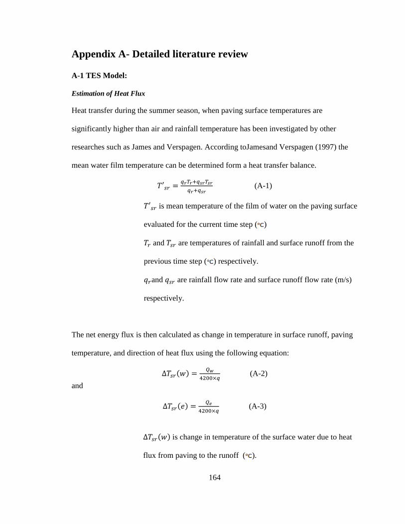
164
Appendix A- Detailed literature review
A-1 TES Model:
Estimation of Heat Flux
Heat transfer during the summer season, when paving surface temperatures are
significantly higher than air and rainfall temperature has been investigated by other
researches such as James and Verspagen. According toJamesand Verspagen (1997) the
mean water film temperature can be determined form a heat transfer balance.
(A-1)
is mean temperature of the film of water on the paving surface
evaluated for the current time step ( )
and are temperatures of rainfall and surface runoff from the
previous time step ( ) respectively.
and are rainfall flow rate and surface runoff flow rate (m/s)
respectively.
The net energy flux is then calculated as change in temperature in surface runoff, paving
temperature, and direction of heat flux using the following equation:
(A-2)
and
(A-3)
is change in temperature of the surface water due to heat
flux from paving to the runoff ( ).

165
is change in temperature of the surface water due to
evaporation ( ),
q is flow rater of water (kg/s),
4200 is a heat capacity (W-s/kg/ ) of water between 10-80 , and
is total energy transferred from paving to the overflowing
water (W).
is negative, total energy transferred from paving to the
atmosphere (W).
Change in pavement temperature can be estimated based on its heat capacity using the following
equation
(A-4)
Where:
= average change in pavement temperature ( ) within 10 cm depth
= time step size (sec)
= heat capacity of asphalt ( / )
d = depth of pavement (m)
area = area of pavement ( )
It is assumed that the pavement temperature change is linear within 10 cm pavement
between the surface and the bottom, and it can estimate the average change in pavement
surface temperature:
(A-5)

166
Where: is a change in pavement surface temperature ( )
Heat Exchange between Paving and Film of Water
The heat transfer
( ) from a flat surface to a liquid surface under turbulent conditions can
be calculated using the following relationship:
(A-6)
Where:
and are temperature of the paving and overlaying water
respectively
is average heat transfer coefficient ( / )
can be calculated using the Nusselt number ( ) using the
following equation:
(A-7)
Where: k is thermal conductivity of the overlying fluid (W/m/ )
L is length of water flow over the paving surface
The Nusselt Number is a function of both the Prandtl Number and Reynolds Number and
accordingly the equation for the Nusselt Number varies. For constant heat transfer where Pr is
between 0.6 - 50, as in case of water flow, the Nusselt Number ( ) is
(A-8)

167
A-2 WEP Model:
WEP is a water and heat energy transfer processes model to simulate spatially variable
water and energy processes in watersheds with complex land covers. Model variables are:
Depression storage, soil moisture content, land surface temperature, groundwater tables,
and water stage in rivers. Hydrological and energy processes are expressed in details and
all processes are formulated. Hydrological processes which are formulated include:
Evapotranspiration, infiltration, surface runoff, subsurface runoff, groundwater flow and
groundwater outflow, and river flow. Energy processes consist of: Energy balance and
land surface, short-wave radiation, long-wave radiation, antropogenic energy
consumption, latent heat flux, sensible heat flux, and heat conduction into soil.
A-3 Statistical approach:
An investigation of stormwater thermal enrichment conducted in the Speed River at
Guelph by Xie and James (1993), and a linear relationship between computed mean
stream temperature from May to September (Ts) and percentage imperviousness (I) is
introduced: Ts= 17.0+0.01 I. Other similar equation by Galli (1990) for a headwater
Piedmont stream (Maryland) is: Ts=15.8+0.076 I. Xie derives an empirical equation to
calculate the expected mean temperature of surface runoff over paving:
Tr=3.26+0.828Tpw where Tr is expected mean temperature of surface runoff and Tpw is
temperature of the wet pavement.

168
Appendix B - Sample charts of collected data
Figure B-1 Pond 33 Guelph summer 2011

169
Figure B-2 Pond 53 Guelph summer 2011
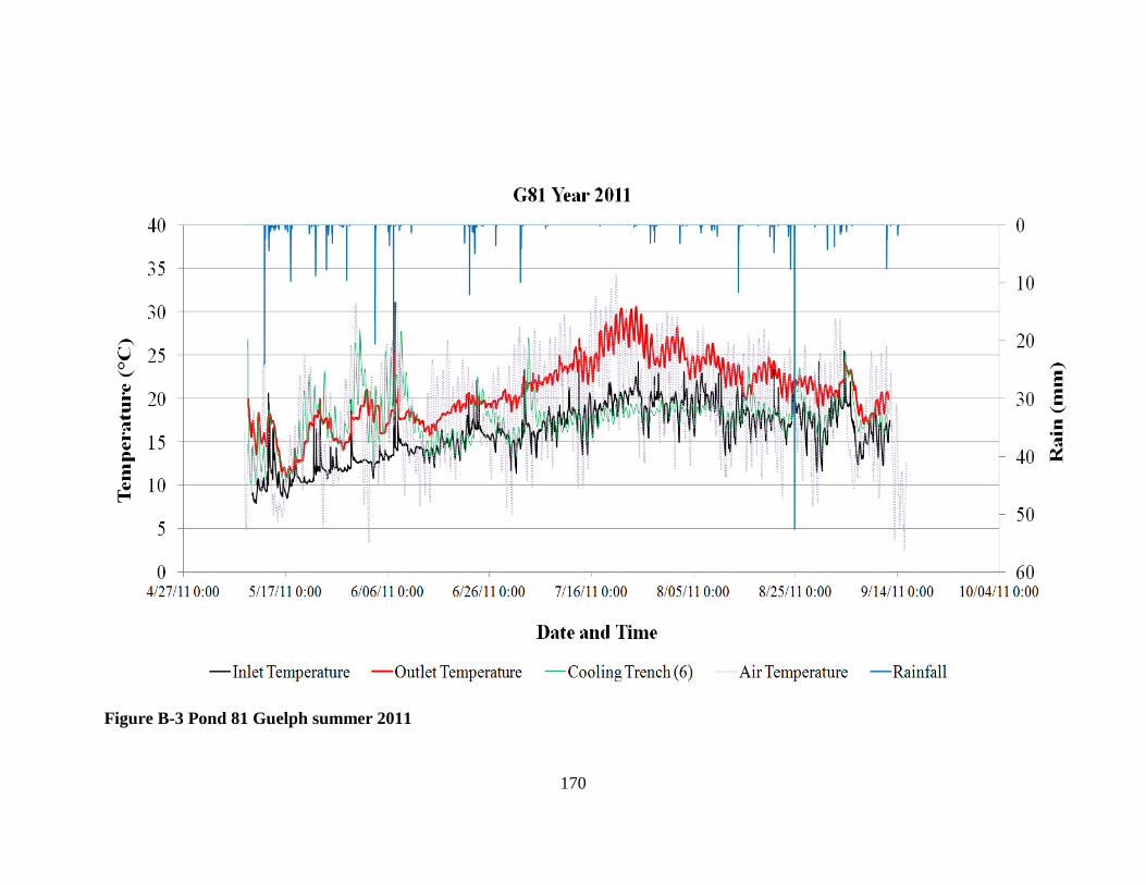
170
Figure B-3 Pond 81 Guelph summer 2011
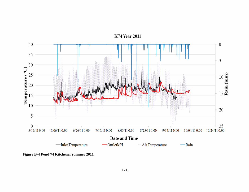
171
Figure B-4 Pond 74 Kitchener summer 2011
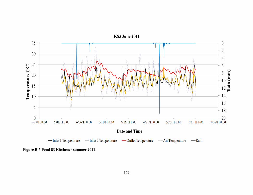
172
Figure B-5 Pond 83 Kitchener summer 2011

173
Figure B-6 Pond Church Kitchener summer 2011

174
Appendix C – Additional Tables Table C-1 Period of Record of data

175
Table C-1 Continue

176
Table C-2 Rainfall-runoff models
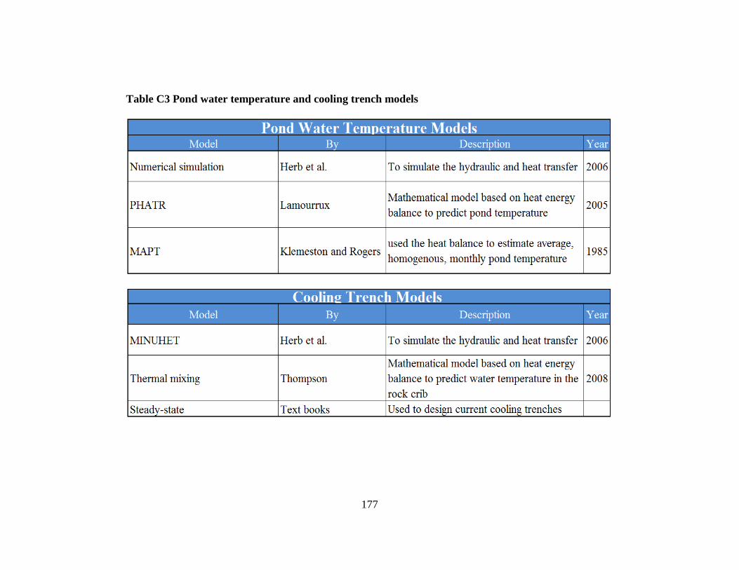
177
Table C3 Pond water temperature and cooling trench models

178
Appendix D – Copyrights Release

179