phase portraits, lyapunov functions, and projective geometry

MATHEMATIK IN DER LEHRE

https://doi.org/10.1007/s00591-020-00288-yMath Semesterber (2021) 68:143–161

Phase portraits, Lyapunov functions, and projectivegeometryLessons learned from a differential equations class and itsaftermath

Lilija Naiwert · Karlheinz Spindler

Received: 16 December 2019 / Accepted: 13 September 2020 / Published online: 19 October 2020© The Author(s) 2020

Abstract We discuss two problems which grew out of an introductory differentialequations class but were solved only later, each after having been put into a differentcontext. First, how do you find a rather complicated Lyapunov function with yourbare hands, without using a fully developed theory (while reconstructing the stepsleading up to such a theory)? Second, how can you obtain a global picture ofthe phase-portrait of a dynamical system (thereby invoking ideas from projectivegeometry)? Since classroom experiences played an important part in the making ofthis paper, didactical aspects will also be discussed.

Keywords Ordinary differential equations · Lyapunov functions · Projectivephase-portraits · Mathematics education

2010 Mathematical Subject Classification: 34A26 · 34D20 · 37C75 · 51N15 ·97D40 · 97E50

1 Introduction

In this paper we reap some late fruit from seeds sown about three years ago, in a classon “Ordinary Differential Equations and Dynamical Systems” which was taught bythe second author and attended by the first author as a third-semester student. Thisclass had an extent of 10 blocks per week of 45 minutes each (usually 6 for lecturesand 4 for lab sessions) and covered the following topics: elementary types of scalar

L. Naiwert · K. Spindler (�)Hochschule RheinMain, Wiesbaden, GermanyE-Mail: [email protected]

L. NaiwertE-Mail: [email protected]

K

https://doi.org/10.1007/s00591-020-00288-y

http://crossmark.crossref.org/dialog/?doi=10.1007/s00591-020-00288-y&domain=pdf

144 L. Naiwert, K. Spindler

differential equations, general formulation of systems of ordinary differential equa-tions, existence and uniqueness theorems, maximal solution intervals, dependenceof solutions on initial data and parameters, variational equations, systems of lineardifferential equations, state transition operator, qualitative theory: phase portraits,equilibria, isoclines, elementary stability theory, Lyapunov functions. (Essentially,chapters 117–124 and 134 from [21] were covered.) There were three written testsduring the semester, focusing on solution techniques and computational skills, andan oral exam at the end of the semester, focusing on conceptual understanding. In theclass, which was attended by about 25 students, a rather exciting and communicativeatmosphere developed, with lots of questions, comments and ideas being broughtup by the students. The two questions discussed in this paper came up in this class,but were settled only later, each after having been put into a different context. Toconvey a flavor of the way the class was taught, we present the topics in the styleof the course, using an example-oriented approach, favoring explicit calculationsbefore introducing more abstract points of view and using pictures and visualiza-tions whenever possible. At the end of the paper, we comment on the classroomexperiences made with this approach and the didactical lessons learned.

2 The search for a Lyapunov function

Consider the system

P� D �2� C 2�;

P� D �2 � �4:(1)

As a routine step to understand the qualitative behavior of this system, we firstdetermine the nullclines and the equilibrium points. The �-nullcline is the line � D � ,the �-nullcline is the union of the two parabolas � D ˙�2, and the equilibria of thesystem, i.e., the points of intersection of these nullclines, are the points .�1; �1/,.0,0/ and .1,1/. Next, again as a routine step, we try to determine the characterof each of these equilibria by linearizing the system about the point in question.Denoting the right-hand side of (1) by f .�; �/, we calculate the derivatives

.Df /.�; �/ D� �2 2�4�3 2�

�; .Df /.�1; �1/ D

��2 24 �2

�;

.Df /.0,0/ D��2 2

0 0

�; .Df /.1,1/ D

��2 2�4 2

�:

(2)

Since .Df /.�1; �1/ has a positive and a negative eigenvalue, we conclude that theequilibrium point .�1; �1/ is unstable for both the linearized and the original system.On the other hand, Df .0,0/ has the eigenvalues –2 and 0, whereas Df .1,1/ has thetwo purely imaginary eigenvalues ˙2i , so that the linearizations of f around .0,0/

and .1,1/ do not help us to determine the character of these equilibrium points.However, completely elementary observations show that both .0,0/ and .1,1/ areunstable.

K

Phase portraits, Lyapunov functions, and projective geometry 145

Fig. 1 Nullclines and qualita-tive sketch of the phase-portraitof the system given by theequations P� D �2� C 2� andP� D �2 � �4

- 2 - 1 1 2

- 1.5

- 1.0

- 0.5

0.5

1.0

1.5

� The green area in Fig. 1 is forward-invariant. A trajectory t 7! ��.t/; �.t/

�starting

in this area satisfies P�.t/ > 0 and P�.t/ > 0 at all times t , so that the functions t 7!�.t/ and t 7! �.t/ are both strictly increasing and, due to invariance, bounded fromabove by zero. This implies that limt!1

��.t/; �.t/

�exists and, being a limit of

a trajectory, must be an equilibrium point, which can only be .0,0/. This shows thateach trajectory starting in the green area tends to .0,0/ as t ! 1. In particular, wecan conclude that .�1; �1/ is unstable without having to invoke the linearizationof the system around this point.

� The blue area in Fig. 1 is also forward-invariant. Arguing in a similar way asbefore, we conclude that if t 7! �

�.t/; �.t/�is a trajectory starting in this area, we

have �.t/ ! �1 and �.t/ ! �1 as t ! 1.� All trajectories originating in the gray triangle in Fig. 1 move upward and to the

right and must either leave this triangle through the top or tend to .1,1/ as t ! 1.Since this holds in particular for trajectories originating arbitrarily close to .0,0/,we conclude that this equilibrium point is unstable.

We can also conclude that there must be a trajectory t 7! ��.t/; �.t/

�converging

to .�1; �1/ as t ! 1. Let us take a quick look at the kind of geometrical andtopological reasoning necessary to establish this claim, as this kind of reasoning wasgreatly appreciated by the students as a contrast to analytically solving differentialequations and as a first experience in deriving qualitative rather than quantitativeinformation. (However, we emphasize that, in general, such elementary argumentsdo not suffice to obtain a full picture of the phase-portrait, but more sophisticatedtools such as the Hartman-Grobman theorem, center manifold theory, the LaSalleinvariance principle or Poincaré-Bendixson theory are required. From a didacticalpoint of view, seeing the limitations of an elementary approach in concrete examplesprovides motivation to study more sophisticated methods.)

K


Fig. 2 Topological argument toprove the existence of a trajec-tory approaching the equilibriumpoint .�1; �1/

P1

P2

C1

C2

Q1Q2

S

A

- 2 - 1 1 2

- 1.5

- 1.0

- 0.5

0.5

1.0

Write A WD .�1; �1/, pick any two points P1 on C1 WD f.�; �/ j � < �1g and P2

on C2 WD f.�; ��2/ j �1 < � < 0g, consider the backward trajectories originatingfrom P1 and P2, choose a line segment S D Q1Q2 connecting these trajectoriesand consider the open region � (shown yellow in Fig. 2) bounded by the segmentS , the trajectories Q1P1 and Q2P2, the segment AP1 on C1 and the arc AP2 onC2. A trajectory starting in � can leave this region neither across S (because ofthe direction of the flow) nor across Q1P1 or Q2P2 (because trajectories cannotintersect), hence must either remain in � for all times or leave � across AP1 orAP2. For p D .�0; �0/ 2 S , denote by 'p.t/ D �

�.t/; �.t/�the trajectory starting

at the point p at time t D 0. For i 2 f1,2g, due to the continuous dependenceof the solutions on the initial values, the set of all p 2 S for which 'p leaves� across APi is open in S , and since S , being connected, cannot be written asa disjoint union of two open sets, there must be at least one point p0 2 S suchthat 'p0 remains in � for all times. Write 'p0.t/ D �

�.t/; �.t/�. Then P�.t/ > 0

and P�.t/ < 0 for all times t , so that the functions t 7! �.t/ and t 7! �.t/ are bothmonotonic and bounded, hence must converge to a limit as t ! 1. As before,the point limt!1

��.t/; �.t/

�must be an equilibrium point, and the only one in

question is A D .�1; �1/. This argument shows that there is a system trajectorytending towards .�1; �1/ from above. Similarly, there must be at least one systemtrajectory tending towards .�1; �1/ from below.

This leaves us with the equilibrium point .1,1/. The sketch of the phase-portraitin Fig. 1 suggests that this might be a stable focus into which nearby trajectoriesspiral as t ! 1. This is confirmed by numerically plotting some trajectories (seeFig. 3), but numerical calculations cannot substitute for a formal proof. Thus thisis the main question to be answered in this section: How can we formally provethat .1,1/ is a stable (even locally asymptotically stable) equilibrium? The canonicalway is to construct a suitable Lyapunov function, and general arguments (see [8],Chapter VI, Theorem 51.2) show that such a Lyapunov function must indeed exist.(See [13] for a proof of the relevant theorem and [9] for historical remarks anda reference list concerning converse Lyapunov theorems.) However, these generalarguments are non-constructive and give no hint as to how such a Lyapunov functioncan practically be obtained. So what do we do?

K


Fig. 3 Phase portrait of thesystem given by P� D �2� C 2�and P� D �2 � �4

- 1.5 - 1.0 - 0.5 0.5 1.0 1.5 2.0

- 1

1

2

Since the right-hand side of the differential equation (1) is a polynomial function,it is plausible (but not always successful; see [1]) to try to find a Lyapunov functionwhich is also polynomial (or at least analytic in a vicinity of the equilibrium point).For simplicity’s sake, we change our coordinate system as to make this equilibriumpoint the origin of the new coordinates. Substituting � D 1 C x and � D 1 C y, thesystem (1) becomes

Px D �2x C 2y DW F.x; y/;

Py D �4x C 2y � 6x2 C y2 � 4x3 � x4 DW G.x; y/:(3)

We seek a Lyapunov function V for the equilibrium point .0,0/ of the system (3),which means that V satisfies V.0,0/ D 0 and has a strict local minimum at .0,0/

whereas W WD Vx � F C Vy � G (where subscripts denote partial derivatives) hasa local maximum at .0,0/ (which we prefer to be strict so that we can show localasymptotic stability rather than just stability). Moreover, V should be analytic ina neighborhood of .0,0/. Let V .k/ be the homogeneous part of V of order k; then

K


necessarily V .0/ D 0 and V .1/ D 0 so that V D Pk�2V

.k/. Then W is automaticallyalso analytic, and we have W D P

k�2W.k/ where

W .2/ D V .2/x F .1/ C V .2/

y G.1/;

W .3/ D V .3/x F .1/ C V .3/

y G.1/ C V .2/y G.2/;

W .4/ D V .4/x F .1/ C V .4/

y G.1/ C V .3/y G.2/ C V .2/

y G.3/;

W .5/ D V .5/x F .1/ C V .5/

y G.1/ C V .4/y G.2/ C V .3/

y G.3/ C V .2/y G.4/;

W .6/ D V .6/x F .1/ C V .6/

y G.1/ C V .5/y G.2/ C V .4/

y G.3/ C V .3/y G.4/;

(4)

and so on; the general formula for m � 5 reads

W .m/ D V .m/x F .1/ C V .m/

y G.1/ C V .m�1/y G.2/ C V .m�2/

y G.3/ C V .m�3/y G.4/: (5)

(We note in passing that, for a general system Pz D Az C higher-order terms inRn with the origin as an equilibrium, the symmetric matrices P; Q 2 Rn�n withV .2/.z/ D zT P z and W .2/.z/ D �zT Qz are related by the Lyapunov equationAT P C PA C Q D 0.) In our situation, the quadratic term V .2/ takes the form

V .2/.x; y/ D Ax2 C 2Bxy C Dy2 D Œxy�

�A B

B D

� �x

y

�(6)

where the coefficient matrix is necessarily positive semidefinite, because V hasa local minimum at .0,0/. This means that A � 0, D � 0 and AD � B2. Plugging(6) into the expression for W .2/ given by (4), multiplying out and sorting termsresults in

W .2/.x; y/ D 4 � � � .AC2B/x2 C .A�2D/xy C .B CD/y2�: (7)

Now since W is supposed to have a local maximum at .0,0/, the function W .2/ mustbe negative semidefinite, which requires that A C 2B � 0, B C D � 0 and

0 � �det��2.AC2B/ A�2D

A�2D 2.B CD/

�

D A2 C 4AB C 8B2 C 8BD C 4D2

D .A C 2B/2 C 4.B C D/2:

(8)

This inequality can only be satisfied (and only as an equality, never as a strictinequality) if B D �D and A D �2B D 2D. Plugging these conditions into theformula (6), we find that V .2/.x; y/ D D � .2x2 �2xy Cy2/. Since we want to reuseA; B; C; D as variable names, we write � instead of D and then have the following

K


result: If there is a polynomial (or analytical) Lyapunov function V at all, then itsquadratic component is necessarily of the form

V .2/.x; y/ D � � .2x2 � 2xy C y2/ where � � 0; (9)

and in this case we have W .2/ D 0. But then for W to be negative semidefinite,we must necessarily have W .3/ D 0, because otherwise W .3/ would be indefinite,implying that W cannot have a local maximum at .0,0/. Now the condition W .3/ D 0determines V .3/. In fact, V .3/ has the general form

V .3/.x; y/ D Ax3 C Bx2y C Cxy2 C Dy3 (10)

where, of course, A; B; C; D differ from the variables with the same names usedbefore. Plugging (10) into the expression for W .3/ in (4), multiplying out and sortingterms, we find that

.1=2/ � W .3/.x; y/ D.�3A � 2B C 6�/x3 C .3A � B � 4C � 6�/x2y

C .2B C C � 6D � �/xy2 C .C C 3D C �/y3;(11)

and W .3/ D 0 if and only if the four coefficients on the right-hand side of (11) allvanish, which means that A; B; C; D are solutions of the system

26643 2 0 03 �1 �4 00 2 1 �60 0 1 3

3775

2664

A

B

C

D

3775 D �

2664

661

�1

3775 : (12)

Upon inversion, we find that2664

A

B

C

D

3775 D �

3

2664

�5 6 8 169 �9 �12 �24

�6 6 9 182 �2 �3 �5

3775

2664

661

�1

3775 D �

3

2664

�212�92

3775 : (13)

To avoid fractions, we write � D 3� and obtain the conditions

V .2/.x; y/ D � � .6x2 � 6xy C 3y2/;

V .3/.x; y/ D � � .�2x3 C 12x2y � 9xy2 C 2y3/;(14)

which guarantee that W .2/ D 0 and W .3/ D 0. Now V .4/ has the general form

V .4/.x; y/ D Ax4 C Bx3y C C x2y2 C Dxy3 C Ey4: (15)

(If � > 0 the function V will always have a strict minimum at .0,0/, no matter howV .4/ is chosen, whereas if � D 0 we must in addition require that V .4/ be positive

K


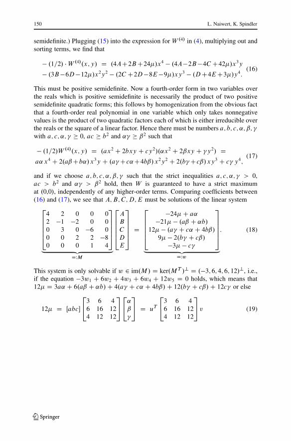
semidefinite.) Plugging (15) into the expression for W .4/ in (4), multiplying out andsorting terms, we find that

� .1=2/ � W .4/.x; y/ D .4AC2B C24�/x4 � .4A�2B �4C C42�/x3y

� .3B �6D �12�/x2y2 � .2C C2D �8E �9�/xy3 � .D C4E C3�/y4:(16)

This must be positive semidefinite. Now a fourth-order form in two variables overthe reals which is positive semidefinite is necessarily the product of two positivesemidefinite quadratic forms; this follows by homogenization from the obvious factthat a fourth-order real polynomial in one variable which only takes nonnegativevalues is the product of two quadratic factors each of which is either irreducible overthe reals or the square of a linear factor. Hence there must be numbers a; b; c; ˛; ˇ; �

with a; c; ˛; � � 0, ac � b2 and ˛� � ˇ2 such that

� .1=2/W .4/.x; y/ D .ax2 C 2bxy C cy2/.˛x2 C 2ˇxy C �y2/ Da˛ x4 C 2.aˇCb˛/x3y C .a� Cc˛C4bˇ/x2y2 C 2.b� Ccˇ/xy3 C c� y4;

(17)

and if we choose a; b; c; ˛; ˇ; � such that the strict inequalities a; c; ˛; � > 0,ac > b2 and ˛� > ˇ2 hold, then W is guaranteed to have a strict maximumat .0,0/, independently of any higher-order terms. Comparing coefficients between(16) and (17), we see that A; B; C; D; E must be solutions of the linear system

266664

4 2 0 0 02 �1 �2 0 00 3 0 �6 00 0 2 2 �80 0 0 1 4

377775

„ ƒ‚ …DWM

266664

A

B

C

D

E

377775 D

266664

�24� C a˛

�21� � .aˇ C ˛b/

12� � .a� C c˛ C 4bˇ/

9� � 2.b� C cˇ/

�3� � c�

377775

„ ƒ‚ …DWw

: (18)

This system is only solvable if w 2 im.M / D ker.M T /? D .�3; 6; 4; 6; 12/?, i.e.,if the equation �3w1 C 6w2 C 4w3 C 6w4 C 12w5 D 0 holds, which means that12� D 3a˛ C 6.aˇ C ˛b/ C 4.a� C c˛ C 4bˇ/ C 12.b� C cˇ/ C 12c� or else

12� D Œabc�

243 6 46 16 124 12 12

35

24˛

ˇ

�

35 D uT

243 6 46 16 124 12 12

35 v (19)

K


where u WD .a; b; c/T and v WD .˛; ˇ; �/T . A straightforward Gaussian eliminationthen yields A; B; C; D; E in terms of �, u and v. In summary, we arrive at theequations

� D 1

12uT

243 6 46 16 124 12 12

35v;

A D 4E � 4� � 1

6uT

240 3 13 4 61 6 0

35v D 4E � 1

2uT

242 5 35 12 103 10 8

35v;

B D �8E � 4� C 1

6uT

243 6 26 8 122 12 0

35v D �8E � 1

2uT

241 2 22 8 42 4 8

35v;

C D 8E C 17

2� � 1

12uT

243 6 46 16 244 24 0

35v D 8E C 1

8uT

2415 30 2030 80 5220 52 68

35v;

D D �4E � 4� C 1

12uT

243 6 46 16 124 12 0

35v D �4E � 1

4uT

243 6 46 16 124 12 16

35v

(20)

in which E can be arbitrarily chosen, reflecting the fact that M has the one-dimen-sional kernel ker.M / D R .4; �8; 8; �4,1/T . Now it is obvious that the number �

defined by (19) is automatically nonnegative if a; b; c; ˛; ˇ; � � 0. Moreover, sincethe matrix occurring in (19) is positive definite (with eigenvalues 0 < �1 < �2 < �3

given by �1 � 0.492, �2 � 2.304 and �3 � 28.204), we conclude that � is nec-essarily positive if .˛; ˇ; �/ D .a; b; c/ ¤ .0; 0; 0/ even if ˇ D b < 0. However,something much more general is true: Whenever the conditions a; c; ˛; � � 0,ac � b2 and ˛� � ˇ2 are satisfied, then the number � defined by (19) is au-tomatically nonnegative, and it is strictly positive unless .a; b; c/ D .0; 0; 0/ or.˛; ˇ; �/ D .0; 0; 0/. (This can be established by denoting the right-hand side of(19) by f .a; b; c; ˛; ˇ; �/ and then determining the minimum of f under the con-straints a; b; ˛; � � 0, ac � b2 and ˛� � ˇ2, distinguishing various cases as towhich of the constraints are active.) Thus we arrive at the following result (which,as we emphasize, is of a purely local character).

Proposition If V is an analytic Lyapunov function for the equilibrium point .0,0/ ofEq. (3), then there are numbers a, b, c, ˛, ˇ, � satisfying the inequalities a; c; ˛; � �0, ac � b2 and ˛� � ˇ2 and a real number E such that

V .2/.x; y/ D � � .6x2 � 6xy C 3y2/;

V .3/.x; y/ D � � .�2x3 C 12x2y � 9xy2 C 2y3/;

V .4/.x; y/ D Ax4 C Bx3y C C x2y2 C Dxy3 C Ey4

(21)

K


where �; A; B; C; D are determined from (20). Conversely, if a, b, c, ˛, ˇ, � are anynumbers satisfying the strict inequalities a; c; ˛; � > 0, ac > b2 and ˛� > ˇ2, if E

is an arbitrary real number and if �; A; B; C; D are determined from (20), then anyanalytic function V D P

k�2V.k/ satisfying (21) is a strict Lyapunov function.

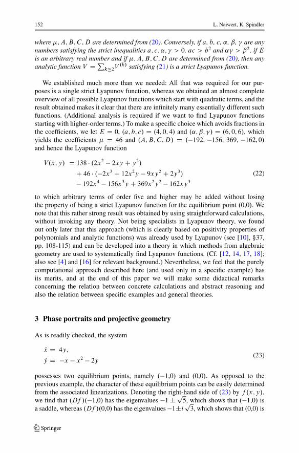
We established much more than we needed: All that was required for our pur-poses is a single strict Lyapunov function, whereas we obtained an almost completeoverview of all possible Lyapunov functions which start with quadratic terms, and theresult obtained makes it clear that there are infinitely many essentially different suchfunctions. (Additional analysis is required if we want to find Lyapunov functionsstarting with higher-order terms.) To make a specific choice which avoids fractions inthe coefficients, we let E D 0, .a; b; c/ D .4; 0; 4/ and .˛; ˇ; �/ D .6; 0; 6/, whichyields the coefficients � D 46 and .A; B; C; D/ D .�192; �156; 369; �162, 0/

and hence the Lyapunov function

V.x; y/ D 138 � .2x2 � 2xy C y2/

C 46 � .�2x3 C 12x2y � 9xy2 C 2y3/

� 192x4 � 156x3y C 369x2y2 � 162xy3

(22)

to which arbitrary terms of order five and higher may be added without losingthe property of being a strict Lyapunov function for the equilibrium point .0,0/. Wenote that this rather strong result was obtained by using straightforward calculations,without invoking any theory. Not being specialists in Lyapunov theory, we foundout only later that this approach (which is clearly based on positivity properties ofpolynomials and analytic functions) was already used by Lyapunov (see [10], §37,pp. 108-115) and can be developed into a theory in which methods from algebraicgeometry are used to systematically find Lyapunov functions. (Cf. [12, 14, 17, 18];also see [4] and [16] for relevant background.) Nevertheless, we feel that the purelycomputational approach described here (and used only in a specific example) hasits merits, and at the end of this paper we will make some didactical remarksconcerning the relation between concrete calculations and abstract reasoning andalso the relation between specific examples and general theories.

3 Phase portraits and projective geometry

As is readily checked, the system

Px D 4y;

Py D �x � x2 � 2y(23)

possesses two equilibrium points, namely .�1,0/ and .0,0/. As opposed to theprevious example, the character of these equilibrium points can be easily determinedfrom the associated linearizations. Denoting the right-hand side of (23) by f .x; y/,we find that .Df /.�1,0/ has the eigenvalues �1 ˙ p

5, which shows that .�1,0/ isa saddle, whereas .Df /.0,0/ has the eigenvalues�1˙i

p3, which shows that .0,0/ is

K


- 1.5 - 1.0 - 0.5 0.5 1.0

- 1.5

- 1.0

- 0.5

0.5

- 2 - 1 1 2 3

- 1.5

- 1.0

- 0.5

0.5

1.0

1.5

2.0

- 4 - 3 - 2 - 1 1 2 3

- 2

- 1

1

2

3

4

- 6 - 4 - 2 2 4

- 2

2

4

6

Fig. 4 Phase-portrait of the system Px D 4y, Py D x � x2 � 2y at different scales

a stable focus. Thus there is no problem in drawing the phase-portrait, and this wasdone by students in the lab sessions of the above-mentioned class, using both handdrawings and computer plots. However, the phase-portraits obtained looked ratherdifferent, depending on the chosen scale. For example, the domain of attraction ofthe equilibrium point .0,0/ looks rather big in the image section shown in the upperleft corner of Fig. 4, but relatively small in the image section shown in the lowerright corner of this figure. Thus the natural question arose how one could be surethat a phase-portrait obtained does not qualitatively change by simply zooming out.In short: How does one get the “big picture”?

The answer to this question, formulated sloppily, is the following: You see moreif you look infinitely far. Thus one complements the phase plane by points at infinityand extends the system to this extended plane. There are different ways of doing so(see [5]); we choose here the Poincaré compactification of the plane, also knownas the oriented projective plane (see [22]), which gives us a chance to bring someattention to projective geometry, one of the most beautiful creations of 19th centurymathematics which, unfortunately, has virtually disappeared from the list of coretopics of most mathematics lines of study. The connection between phase-portraitanalysis and projective geometry is not covered in most textbooks; the only excep-tions we are aware of are the graduate-level text [7], the monograph [8] and the two

K


American textbooks [11] and [15]. Thus it may be no waste of time to discuss thistopic here. Let us consider a system of differential equations

Px D P.x; y/

Py D Q.x; y/(24)

with polynomials P and Q. We identify the xy-plane with the plane f.x; y; 1/ 2R3 j x; y 2 Rg. Given .x; y/, the line joining .0; 0; 0/ and .x; y; 1/ intersects thesphere X2 C Y 2 C Z2 D 1 in two antipodal points; the one of these two pointssatisfying Z > 0 is

24X

Y

Z

35 D 1p

1 C x2 C y2

24x

y

1

35 ; (25)

and the equations

x D X

Z; y D Y

Z(26)

show how conversely .x; y/ can be reconstructed from .X; Y; Z/. The further away.x; y/ is from .0,0/, the closer .X; Y; Z/ is to the equator, and thus we interpret pointson the equator as points at infinity. Now just like one forms the projective closureof an algebraic curve in algebraic geometry, one can ask which points at infinitylie on a solution curve of a system of differential equations. If t 7! �

x.t/; y.t/�

is a trajectory of (24), then the corresponding image curve t 7! �X.t/; Y.t/; Z.t/

�satisfies the following system of differential equations:

PX D Px.1Cy2/ � xy Py.1Cx2Cy2/3=2

D Z3 ��P

�X

Z;

Y

Z

�� Z2CY 2

Z2� XY

Z2� Q

�X

Z;

Y

Z

��

D Z ��.Y 2CZ2/ � P

�X

Z;

Y

Z

�� XY � Q

�X

Z;

Y

Z

��;

PY D Py.1Cx2/ � xy Px.1Cx2Cy2/3=2

D Z3 ��Q

�X

Z;

Y

Z

�� Z2CX2

Z2� XY

Z2� P

�X

Z;

Y

Z

��

D Z ��.X2CZ2/ � Q

�X

Z;

Y

Z

�� XY � P

�X

Z;

Y

Z

��;

PZ D �x Px � y Py.1Cx2Cy2/3=2

D �Z3 ��P

�X

Z;

Y

Z

�� X

ZC Q

�X

Z;

Y

Z

�� Y

Z

�

D �Z2 ��X � P

�X

Z;

Y

Z

�C Y � Q

�X

Z;

Y

Z

��:

(27)

This can be easily seen by first taking derivatives in (25), then plugging in thesystem equations (24) and finally expressing x; y in terms of X; Y; Z using (26).Now let m be the highest degree of any of the monomials constituting P and Q.

K


Concretely: Combining in the expressions for P and Q terms of equal order, weobtain representations

P.x; y/ D P0.x; y/ C P1.x; y/ C � � � C Pm�1.x; y/ C Pm.x; y/;

Q.x; y/ D Q0.x; y/ C Q1.x; y/ C � � � C Qm�1.x; y/ C Qm.x; y/;(28)

where at least one of the polynomials Pm and Qm is different from zero. If we nowdefine

P ?.X; Y; Z/ WD Zm � P

�X

Z;

Y

Z

�and

Q?.X; Y; Z/ WD Zm � Q

�X

Z;

Y

Z

�;

(29)

the equations (27) take the form

PX D .Y 2 C Z2/ � P ?.X; Y; Z/ � XY � Q?.X; Y; Z/

Zm�1;

PY D .X2 C Z2/ � Q?.X; Y; Z/ � XY � P ?.X; Y; Z/

Zm�1;

PZ D �X � P ?.X; Y; Z/ C Y � Q?.X; Y; Z/

Zm�2:

(30)

We see that the factor 1=Zm�1 occurs in all three expressions on the right-hand sideof (30). To eliminate this factor, we carry out a substitution WD .t/ such that

d

dtD 1

Z.t/m�1(31)

and treat as a new time variable. Intuitively this means that we change the speedwith which the curves (30) are traversed: The smaller Z is (i.e., the further theoriginal curve tends to infinity), the bigger are the time steps, i.e., the slower webecome. Denoting derivatives with respect to by primes (whereas derivatives withrespect to t are denoted by dots) and applying the chain rule, we find that

PX D dX

dtD dX

d� d

dtD X 0 � 1

Zm�1;

PY D dY

dtD dY

d� d

dtD Y 0 � 1

Zm�1;

PZ D dZ

dtD dZ

d� d

dtD Z 0 � 1

Zm�1:

(32)

K


Thus the equations (30) become

X 0 D .Y 2 C Z2/ � P ?.X; Y; Z/ � XY � Q?.X; Y; Z/;

Y 0 D .X2 C Z2/ � Q?.X; Y; Z/ � XY � P ?.X; Y; Z/;

Z 0 D �Z � �X � P ?.X; Y; Z/ C Y � Q?.X; Y; Z/

�:

(33)

For this new system (33) the equator Z D 0 (or equivalently X2 C Y 2 D 1) is nolonger a singular set, but simply an invariant set on which the system dynamics areseen to be given by

X 0 D Y 2 � P ?.X; Y; 0/ � XY � Q?.X; Y; 0/

Y 0 D X2 � Q?.X; Y; 0/ � XY � P ?.X; Y; 0/(34)

by plugging in Z � 0 into (33). Now (28) implies

P

�X

Z;

Y

Z

�D P0.X; Y / C P1.X; Y /

ZC � � � C Pm�1.X; Y /

Zm�1C Pm.X; Y /

Zm(35)

and hence

P ?.X; Y; Z/ DZmP

�X

Z;

Y

Z

�D ZmP0.X; Y / C Zm�1P1.X; Y /

C Zm�2P2.X; Y / C � � � C Z Pm�1.X; Y / C Pm.X; Y /I(36)

in particular we see that P ?.X; Y; 0/ D Pm.X; Y /. A completely analogous resultholds for Q?. Thus (34) becomes

X 0 D Y 2 � Pm.X; Y / � XY � Qm.X; Y /

Y 0 D X2 � Qm.X; Y / � XY � Pm.X; Y /(37)

which means that�X 0Y 0

�D �

XQm.X; Y / � Y Pm.X; Y /� ��Y

X

�: (38)

Because of the equation X2CY 2 D 1 it is not possible that X and Y simultaneouslytake the value zero. Hence the only equilibria of (38) are the solutions .X; Y / of theequation

XQm.X; Y / � Y Pm.X; Y / D 0. (39)

Thus this equation yields the equilibria at infinity. What has been done here canbe summarized as follows. To every polynomial system on R2 one can associatea system on S2C (i.e., the open upper hemisphere Z > 0) such that there is a one-to-one correspondence between the trajectories of both systems (via the standard pull-back/push-forward of the corresponding vector fields). The resulting system on S2C

K


can then be extended (possibly after rescaling the time variable) to the closure S2C(i.e., to the closed upper hemisphere Z � 0). The flow on the equator Z D 0, givenby (39), is then invariant for the extended system and characterizes the flow of theoriginal system “at infinity”; cf. Theorem 1 in [15], Sect. 3.10. We note that thereare other ways to analyze the flow of the original system “at infinity”, for exampleBendixson’s approach of using the standard one-point compactification ofR2. Usingthe Poincaré sphere can be regarded as a way of “blowing up” the singularity at “1”which would be obtained by Bendixson’s approach, which has the disadvantage thatthe complete behavior of the original flow “at infinity” is concentrated in one singlepoint (around which the induced flow can be very complicated) rather than beingspread out along the equator. (See the remarks on p. 268 in [15].)

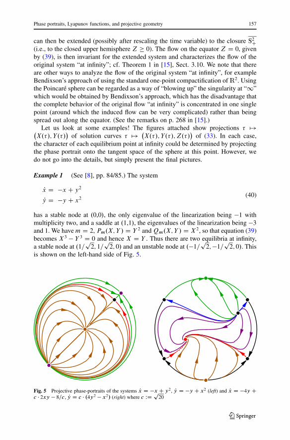
Let us look at some examples! The figures attached show projections 7!�X./; Y./

�of solution curves 7! �

X./; Y./; Z./�of (33). In each case,

the character of each equilibrium point at infinity could be determined by projectingthe phase portrait onto the tangent space of the sphere at this point. However, wedo not go into the details, but simply present the final pictures.

Example 1 (See [8], pp. 84/85.) The system

Px D �x C y2

Py D �y C x2(40)

has a stable node at .0,0/, the only eigenvalue of the linearization being �1 withmultiplicity two, and a saddle at .1,1/, the eigenvalues of the linearization being �3and 1. We have m D 2, Pm.X; Y / D Y 2 and Qm.X; Y / D X2, so that equation (39)becomes X3 � Y 3 D 0 and hence X D Y . Thus there are two equilibria at infinity,a stable node at .1=

p2; 1=

p2; 0/ and an unstable node at .�1=

p2; �1=

p2; 0/. This

is shown on the left-hand side of Fig. 5.

Fig. 5 Projective phase-portraits of the systems Px D �x C y2, Py D �y C x2 (left) and Px D �4y Cc � 2xy � 8=c, Py D c � .4y2 � x2/ (right) where c WD p

20

K


Fig. 6 Projective phase-portraitof the system Px D 4y, Py D�x � cx2 � 2y where c WD 3

Example 2 (See [11], pp. 236-238.) The system

Px D �4y C 2xy � 8

Py D 4y2 � x2 (41)

has an unstable node at .4,2/, the eigenvalues of the linearization being 8 and 12,and a stable focus at .�2; �1/, the eigenvalues of the linearization being �5˙i

p23.

We have m D 2, Pm.X; Y / D 0 and Qm.X; Y / D 4Y 2 � X2, so that equation (39)becomes Y.2Y �X/.2Y CX/ D 0 with the three solutions Y D 0 and Y D ˙X=2.Consequently, there are six equilibria at infinity, namely nodes at .0; ˙1,0/ andsaddles at .˙p

2=3; ˙p1=3; 0/. This is shown on the right-hand side in Fig. 5. To

obtain a visually appealing presentation, we used the scaling .x; y/ 7! .x=c; y=c/

with the factor c WD p20.

Example 3 This is the system (23) with which we started our discussion. Wehave m D 2, Pm.X; Y / D 0 and Qm.X; Y / D X2, so that equation (39) reduces toX3 D 0 and hence X D 0. Thus there are two equilibria at infinity, namely a stablenode at .0; �1,0/ and an unstable node at .0; 1; 0/. This is shown in Fig. 6, whichcan be considered as the limiting case of the diagrams in Fig. 4 as the image sectionconsidered gets infinitely large. Again, we used a scaling .x; y/ 7! .x=c; y=c/, thistime with the factor c D 3, to improve the graphical output.

We emphasize that passing from the real plane to its Poincaré compactificationis merely a way of seeing the phase-portrait of a planar system on a global scale,but does not eliminate the need for other methods to reveal the details of this phase-portrait.

K


4 Didactical issues and classroom experiences

Let us discuss some of the didactical issues which played a role in both the genesisof this paper and the differential equations class from which it emerged.

Subject matter: Didactical issues in mathematics education cannot be separatedfrom the subject at hand, and the study of differential equations and dynamicalsystems is a particularly attractive and rewarding topic, combining mathematicalmethods with interesting applications in mechanics, optics, biology, medicine, eco-nomics and other disciplines, blending computational and conceptual aspects anddrawing on prerequisites from various different other disciplines (analysis, linearalgebra, mathematical structures, point mechanics). The students appreciated beingable to apply and consolidate what they had learned in previous semesters and seeingconnections between hitherto separated topics, a prominent example being the useof the exponential function for matrices. The ample time available for the courseallowed for the inclusion of all of these different facets.

Example-oriented approach: In our experience, students find it encouraging totry their hands on specific examples before being exposed to the development ofa general theory. (In fact, it seems to be a common mistake in teaching mathematicsto provide answers to questions the students have not even thought to ask.) Well-chosen examples can provide motivation and a hands-on feeling for the subjectmatter, and they can stimulate the wish to replace ad hoc arguments and lengthycalculations by general arguments. A mathematical theory, however elegant it maybe, is not understood without having relevant examples in mind.

Numerical calculations: Students usually like doing concrete calculations, andthey are not in bad company in this regard: Great mathematicians like Newton,Euler, Gauß or Jacobi did not shy away from extremely tedious calculations. (Ina famous instance Newton, after determining the first 16 decimal places of , some-what sheepishly wrote: “I am ashamed to tell you to how many figures I carriedthese computations, having no other business at the time.” See [23], p. 133, quotedfrom [20], p. 219.) While – arguably – it may ultimately be the goal of mathematicsto replace explicit computations by conceptual arguments, such computations havetheir place in mathematics education, providing a hands-on feeling, a sense for thenumerical difficulties inherent in a given problem and, especially if tedious andcumbersome, a strong motivation for the development of a general theory.

Visualization: From our experience, the usefulness of visualizing mathematicalcircumstances can hardly be overestimated. For example, in the differential equa-tions class which gave rise to this paper, both sketching phase-portraits of dynamicalsystems by hand and using mathematical software to produce more accurate com-puter plots formed an essential part of the course, with positive effects not only ongeometrical thinking and programming skills, but also on a deeper understandingof dynamical systems, since creating good plots requires not only computer skills,but also mathematical considerations. Besides that, the positive impact of the mereaesthetical effect of a nicely drawn diagram should not be underestimated.

Perseverance: The problems discussed in this paper came up in a third-semesterdifferential equations class, but they were not solved in this class, but left unsettleduntil later. The problem of finding a suitable Lyapunov function for the equilibrium

K


point in question was taken up by the first author when studying the article [19]and realizing the applicability of optimality criteria for polynomials to this problem;see [2, 3 and 6] for relevant background. Similarly, the possibility of applying ideasfrom projective geometry to better understand phase-portraits of dynamical systemsoccurred to the second author only later, while preparing a geometry class. Thusin both cases the solution ideas sprang to mind due to being placed in a differentcontext and suddenly seeing a connection hidden before: When new topics andmethods were studied, the mind was prepared to apply these new methods to the oldproblems. (As Louis Pasteur observed, chance favors the prepared mind.) Seeingconnections between formerly unrelated fields – differential equations, algebraicgeometry, projective geometry – induced in us excitement and a feeling for thegeneral unity of mathematics.

Funding Open Access funding enabled and organized by Projekt DEAL.

Open Access This article is licensed under a Creative Commons Attribution 4.0 International License,which permits use, sharing, adaptation, distribution and reproduction in any medium or format, as long asyou give appropriate credit to the original author(s) and the source, provide a link to the Creative Com-mons licence, and indicate if changes were made. The images or other third party material in this articleare included in the article’s Creative Commons licence, unless indicated otherwise in a credit line to thematerial. If material is not included in the article’s Creative Commons licence and your intended use is notpermitted by statutory regulation or exceeds the permitted use, you will need to obtain permission directlyfrom the copyright holder. To view a copy of this licence, visit http://creativecommons.org/licenses/by/4.0/.

References

1. Ahmadi, A.A., El Khadir, B.: A globally asymptotically stable polynomial vector field with rationalcoefficients and no local polynomial Lyapunov function. Syst. Control Lett. 121, 50–53 (2018)

2. Barone-Netto, A.: Jet-Detectable Extrema. Proc. Am. Math. Soc. 92(4), 604–608 (1984)3. Barone-Netto, A., Gorni, G., Zampieri, G.: Local extrema of analytic funtions. Nonlinear Differ. Equa-

tions Appl. 3, 287–303 (1996)4. Basu, S., Pollack, R., Roy, M.-F.: Algorithms in real algebraic geometry. Springer, Berlin, Heidelberg

(2010)5. Behnke, H.: Über die verschiedenen Möglichkeiten, in der ebenen Geometrie unendlich ferne Punkte

einzuführen. Math Semesterber 63, 171–185 (2016)6. Bierstone, E., Milman, P.D.: Semianalytic and subanalytic sets. Publ. Mathem. l’I.H.É.S 67, 5–42

(1988)7. Dumortier, F., Llibre, J., Artés, J.C.: Qualitative theory of planar differential systems. Springer, Berlin

Heidelberg (2006)8. Hahn, W.: Stability of motion. Springer, New York (1967)9. Christopher, M.: Classical converse theorems in Lyapunov’s second method. Discrete Continuous Dyn.

Syst. Ser. B. 20(8), 2333–2360 (2015)10. Malkin, J.G.: Theorie der Stabilität einer Bewegung. Akademie-Verlag, Berlin (1959)11. Meiss, J.D.: Differential Dynamical Systems. Society for Industrial and Applied Mathematics,

Philadelphia (2007)12. Malisoff, M., Mazenc, F.: Constructions of strict Lyapunov functions. Springer, London (2009)13. Massera, J.L.: On Liapounoff’s conditions of stability. Ann. Math. 50(3), 705–721 (1949)14. Parrilo, P.A.: Semidefinite programming relaxations for semialgebraic problems. Math. Program. Ser. B

96, 293–320 (2003)15. Perko, L.: Differential equations and dynamical systems, 3rd edn. Springer, New York, Berlin, Heidel-

berg (2001)16. Prestel, A., Delzell, C.: Positive polynomials. Springer, Berlin, Heidelberg (2001)17. Ravanbakhsh, H., Sankaranarayanan, S.: Learning control Lyapunov functions from counterexamples

and demonstrations. Auton. Robots 43, 275–307 (2019)

K

http://creativecommons.org/licenses/by/4.0/

http://creativecommons.org/licenses/by/4.0/


18. Sassi, M.A.B., Sankaranarayanan, S., Chen, X., Ábrahám, E.: Linear relaxations of polynomial posi-tivity for polynomial Lyapunov function synthesis. IMA J. Math. Control Inf. 33(3), 723–756 (2016)

19. Scheeffer, L.: Theorie der Maxima und Minima einer Function von zwei Variabeln. Math. Ann. 25(4),541–576 (1890)

20. Sonar, T.P.M., et al.: The history of the priority dispute between Newton and Leibniz: Mathematics inhistory and culture. Birkhäuser, Cham, Switzerland (2018)

21. Spindler, K.: Höhere Mathematik: Ein Begleiter durch das Studium. Harri Deutsch, Frankfurt (2010)22. Stolfi, J.: Oriented projective geometry – A framework for geometric computations. Academic Press,

San Diego (2014)23. Turnbull, H.W. (ed.): The correspondence of Isaac Newton vol. 2, pp 1676–1687. Cambridge University

Press, Cambridge (1960)

K

phase portraits, lyapunov functions, and projective geometry

Documents