phase-out and disposal issues of obsolete inventory items … · 2018-02-17 · phase-out and...
TRANSCRIPT

PHASE-OUT AND DISPOSAL ISSUES OF OBSOLETE INVENTORY ITEMS IN RETAIL STORES
A Dissertation Presented by
Nizar Zafer Zaarour
to The Department of Mechanical and Industrial Engineering
In partial fulfillment of the requirements for the degree of
Doctor of Philosophy
In the field of Industrial Engineering
Northeastern University Boston, Massachusetts
June 2011

© Copyright 2011 by Nizar Zaarour All Rights Reserved

Page i
Preface and Acknowledgments
At the end of this journey, one might think that this is the time of reflection and
remembering all the long nights, the hardship, the people that doubted and questioned my ability
of making it through. But everything has an end, and when it comes, it is only the beginning of
something else.
Life is a function of time, and this is the time to be thankful to all the people that have
impacted this journey in a positive way and to look forward to the next adventure. I want to
dedicate this to the person that has been my most important supporter as well as being my most
influential inspiration, my mom. She has been the only constant among all the variables of life.
I would like to thank the usual suspects, my dad, my sister, the rest of the family and
friends, and my committee members for their support and help in the last few years. Starting
with my advisor, professor Melachrinoudis for encouraging me to get into the PhD program and
for putting up with me for all these years, to professor Solomon, for being a major positive
impact not only on my academic advancement, but on my professional one as well, and to
professor kamarthi, for agreeing to join the committee and supporting the push towards the finish
line. I also want to send special thanks to Allan Barr for supplying the field data, and to
Alexandra for volunteering to edit all the grammatical errors without realizing what she was
getting herself into. I also want to send a special shut-out to all the ex-huskies that have
accompanied me along the way, to the undergrad gang: Bill, Rick, Todd, Mike, Ed, Chad, Matt,
and Mark; and to my grad crew: Victor, Sameer, Chris, and Gilan.
“No man can reveal to you aught but that which already lies half asleep in the dawning of
our knowledge. The teacher who walks in the shadow of the temple, among his followers, gives

Page ii
not of his wisdom but rather of his faith and his lovingness. If he is indeed wise he does not bid
you enter the house of wisdom, but rather leads you to the threshold of your own mind.
The astronomer may speak to you of his understanding of space, but he cannot give you his
understanding. The musician may sing to you of the rhythm which is in all space, but he cannot
give you the ear which arrests the rhythm nor the voice that echoes it. And he who is versed in
the science of numbers can tell of the regions of weight and measure, but he cannot conduct you
thither. For the vision of one man lends not its wings to another man. And even as each one of
you stands alone in God's knowledge, so must each one of you be alone in his knowledge of God
and in his understanding of the earth” (Gibran, 1923).
Education, in other words, is a way of life and not a personal goal. It is not a discrete
variable that gets measured by getting degrees, but a continuous variable that lasts for the
duration of one’s life.
Z.A.F.

Page iii
Abstract
Logistics is the management of the flow of goods, information and other resources
between the point of production and the point of consumption in order to meet the requirements
of consumers. Logistics involves mainly the integration of information, transportation, and
inventory.
This dissertation addresses two important issues of the multifaceted area of logistics. The
first pertains to inventory management and focuses on the problems of when and by how much
to discount products that are being phased-out due to non-sales or the manufacturer’s /
distributor’s decision. The second issue tackled is the transportation aspect of the reverse
logistics problem which will aim to handle the remaining products returned by the consumer to
the distributor or the manufacturer.
Often times, items in retail stores are phased-out due to the introduction of replacement
items from the distributor. In order to sell out these items within a certain time horizon, retail
stores need to develop markdown strategies. In the first phase of this dissertation, an optimal
markdown strategy is developed as a primary step using a multi-period nonlinear programming
model. Based on price elasticity of demand, the model maximizes revenue from the
discontinued items. The mathematical properties of the model are established and a closed form
optimal solution of the model is found. Furthermore, this model is tested with real data provided
by a retailer. In the second step of this phase, a linear model is developed to address the issues of
when and for how long to apply pre-determined markdown strategies during the phase-out
period.

Page iv
The second phase of the dissertation deals with the remaining inventory, in the case that
not all items are sold during the phase-out period. A mixed integer nonlinear programming
model that aims to manage product returns from individual retail stores (customers) under
capacity constraints and service requirements is developed. Given the complexity of this model,
a linear transformation of the non-linear objective function is presented. Through computational
experiments, it is shown that the linearization produces better quality solutions and enables the
handling of larger-sized data problems. Closed form solutions are obtained for special structures
of the problem.
Key words: product returns, closed-loop supply chains, linear transformation, phase-out,
elasticity of demand, nonlinear, markdown strategies.

Page v
Contents Preface and Acknowledgments ......................................................................................... i
Abstract ........................................................................................................................... iii
List of Figures ................................................................................................................ vii
List of Tables ................................................................................................................ viii
1 Introduction ...............................................................................................................1
1.1 Overview ..........................................................................................................1
1.2 Motivation ........................................................................................................7
1.3 Research Scope and Contributions .................................................................10
1.4 Dissertation Organization ...............................................................................11
2 Literature Review ...................................................................................................13
2.1 Demand and Pricing Strategies ......................................................................13
2.2 End of Life Products and Clustering Analysis ...............................................18
2.3 Reverse Logistics and Product Returns ..........................................................22
3 Proposed Research ..................................................................................................25
3.1 Deliverables to the Phase-out Models ............................................................25
3.2 Deliverables to the Return Products Model ...................................................30
3.3 Research Objectives .......................................................................................33
4 Solution Methodology .............................................................................................34
4.1 Proposed Solution to the Phase-out Models ...................................................34
4.2 Proposed Solution to the Return Products Model ..........................................45
4.2.1 Linearization of the Model ............................................................................49
5 Special Problem Structures....................................................................................52
5.1 Markdown Strategies Analysis .......................................................................52
5.2 Determining the Optimal Collection Period in the Reverse Logistics Model 58
5.2.1 Special Structures of the Optimal Collection Period Problem ......................60
6 Computational Results ...........................................................................................66
Page vi
6.1 Clustering Procedures and Regression Analysis ............................................66
6.2 Inventory Depletion and Markdown Strategies within a Phase-out Period ...71
6.3 Computational Results of the Reverse Logistics Model ................................77
6.4 Sensitivity Analysis ........................................................................................80
7 Summary and Recommendations for Future Research ......................................84
7.1 Recommendations for Future Research .........................................................85
Appendix A: Reverse Logistics Lingo Model ................................................................87
Appendix B: Clustering Algorithm Lingo Model .........................................................89
Appendix C: Price Elasticity Lingo Model ....................................................................90
Appendix D: Initial Data Set for the Reverse Logistics Model ....................................91
Appendix E: Solution Summary for the Reverse Logistics Model ..............................93
Appendix F: Initial Data Set for the 6 Cosmetics SKUs ..............................................94
Appendix G: Reverse Logistics Mock-Up ....................................................................106
Appendix H: Normality Test for all 6 SKUs ...............................................................107
Index ................................................................................................................................114
List of Abbreviated Terms ............................................................................................115
References .......................................................................................................................116
Additional Book References ..........................................................................................121
Page vii
List of Figures
Figure 1: Elasticity of demand ................................................................................... 2
Figure 2: Elastic demand vs. price ............................................................................. 2
Figure 3: Perfect elastic demand ................................................................................ 3
Figure 4: Inelastic demand vs. price ........................................................................... 3
Figure 5: Perfect inelastic demand ............................................................................. 3
Figure 6: Phase-out process ........................................................................................ 4
Figure 7: Different scaling to the same type of data ................................................ 21
Figure 8: Effect of different values for the price elasticity of demand .................... 27
Figure 9: Unit transportation cost function .............................................................. 48
Figure 10: Transportation cost function ..................................................................... 51
Figure 11: Rate of change of revenue with respect to change in volume ................... 57
Figure 12: Simplified unit transportation cost function ............................................. 59
Figure 13: Unit price vs. total sales volume for a particular SKU ............................. 68
Figure 14: Cluster means (unit price) vs. total sales volume for a particular SKU .... 69
Figure 15: Comparison of the power functions of the different SKUs ...................... 70
Figure 16: Optimal periods in discrete vs. continuous T ............................................ 83

Page viii
List of Tables
Table 1: The impact of product returns on the industry-wide revenue ..................... 6
Table 2: Interpretation of the price elasticity coefficient (β) .................................. 27
Table 3: Final selection of SKUs to be analyzed .................................................... 67
Table 4: K-means algorithm results ........................................................................ 69
Table 5: As Unit price decreases, volume increases ............................................... 70
Table 6: Optimal prices / maximum revenue at the end of the phase-out period ... 72
Table 7: Lowest values of salvage price C .............................................................. 73
Table 8: Pre-determined markdown prices ............................................................. 74
Table 9: Determining when and for how long to use the markdown prices ........... 75
Table 10: Model results using I/T and C ................................................................... 75
Table 11: Input parameters to the reverse logistics model ........................................ 78
Table 12: Remaining inventory of the SKU in question broken down by store ....... 79
Table 13: Cost breakdown and comparison of model results ................................... 80
Table 14: Behavior of T as the number of customers increases ............................... 82

Page 1
Chapter 1
Introduction
This chapter provides an introduction to the dissertation. Section 1.1 presents an
overview of the main topics to be discussed, and the important logistic problems that this
dissertation aims to resolve. Section 1.2 presents a description into the motivation behind the
work and the research performed in this field. Section 1.3 provides a general scope of the
problem and the contribution that this dissertation aims to make. Lastly, Section 1.4 outlines the
research and breaks down the main objectives.
1.1 Overview
“The higher the price, the less you will buy” is one of the most famous concepts in
economics. To predict consumer behavior, economists use well-defined techniques, evaluating
consumers’ sensitivity to changes in price; the most commonly used measure is the “price
elasticity of demand.” Elasticity of demand is the ratio of the percentage of the change in
demand with respect to the percentage of the change in price as shown in Figure 1: Ed = (%
change in quantity demanded / % change in price) = PP
/
/

D
price for
demand f
a product
G
large dec
flatter (a
or service
Demand for a
the product
for the produ
t is sold and
Generally spe
crease in the
s shown bel
e in question
F
a product ca
. Inelastic d
uct; elastic d
will not buy
eaking, the d
e quantity de
low in Figur
n is elastic.
Fi
Figure 1: E
an be said to
demand allow
demand exist
y if the price
demand curv
emanded wit
re 3), or mor
igure 2: Ela
lasticity of d
o be very ine
ws a produc
ts when cons
e rises by wh
ve has a neg
th a small in
re horizonta
stic demand
demand
elastic if con
cer to raise p
sumers are s
hat they cons
gative slope
ncrease in pr
al. This flatte
d vs. price
nsumers wil
prices withou
sensitive to t
sider excessi
e (Figure 2),
rice, the dem
er curve mea
P
ll pay almos
ut much affe
the price at w
ive.
and if there
mand curve
ans that the
age 2
st any
ecting
which
e is a
looks
good

M
and 5) as
Meanwhile, i
s quantity ch
F
inelastic dem
hanges little w
Fig
Fi
Figure 3: Pe
mand is repr
with a large
gure 4: Inela
gure 5: Per
rfect elastic
resented wit
movement i
astic deman
fect inelasti
c demand
th a much m
in price.
nd vs. price
ic demand
more upright
P
t curve (Fig
age 3
ure 4

Page 4
In the first stage of this dissertation, changes in demand for items that are being phased-
out will be addressed. Once a retailer learns that an item is being discontinued, the question
becomes: What are the best prices during the different phase-out periods in order to deplete the
given initial inventory on time? The problem of “when” and “by how much” to markdown is
always present. Making wrong decisions could result in unsatisfactory consequences for
retailers, for example a surplus of unnecessary inventory or worse, a loss in profits. In addition,
the problems of the phase-out process will be looked at from a different perspective, where the
markdown prices will be fixed and the questions of “when” and for “how long” to discount at
each pre-determined price will be resolved. Figure 6 below depicts the phase-out process, with
an initial inventory to be depleted at the beginning of the phase-out period, and either no
inventory or a remaining inventory at the end of the fixed phase-out period.
Figure 6: Phase-out process
T represents that phase-out period, I0 is the initial inventory and r is the final remaining
inventory.
Real data from a retailer is used as primary information for this research. In order to
address the key problem at hand, consideration is given to the life of a particular product over a
period of 54 weeks and its behavior through price changes. Subsequently, the product life period
r = 0
r > 0
Beginning of phase-out T is finite
I0
End of phase-out

Page 5
is narrowed down by using a clustering analysis method. The clustered data are fit into a
nonlinear regression model. As a result, this model type is the same used to illustrate the price
elasticity of demand. Based on that model, the behavior of an obsolete inventory item over a
certain phase-out period can be predicted. Given an initial inventory to be depleted, the best
price for each period can be determined in order to maximize revenue. In the case that the whole
initial inventory is unable to be entirely depleted, and the option, to sell the remaining inventory
to a third party retailer with a particular salvage price is present, the model is modified to
determine that remaining amount of inventory, and to determine the new optimal prices for each
period in order to maximum revenue. The last approach deals with the problem of when and for
how long to discount if the markdown prices are pre-determined. A new model is developed to
address at what stage in the phase out period a particular discount should be applied and do all
the different values of discounts get used when trying to obtain the objective function of
maximizing our profit.
The second phase of the dissertation focuses on the management of the remaining
products that have neither been sold during the phase-out period nor have been sold to a third
party. This is an area of reverse logistics. Returned products come in all different sizes, shapes,
and conditions and they are more difficult and costly to handle than original products. In fact, the
logistics of handling returned products accounts for nearly 1% of the total U.S. gross domestic
product (Gecker, 2007). To elaborate further, a study conducted by the Reverse Logistics
Executive Council reported that U.S. companies spent more than $35 billion annually on the
handling, transportation, and processing of returned products (Meyer, 1999). This estimate does
not even include disposition management, administration time, and the cost of converting
impaired materials into productive assets. In some industries such as e-tailing, apparel, and book

Page 6
sales where return rates are usually high, the company’s capability to manage its returned
products may dictate its competitiveness. Though less dramatic, other industries in which return
rates are nominal can suffer significantly from poor return management (see Table 1). For
example, in the industrial equipment sector where return rates typically run 4-8%, its total
revenue can be adversely affected with a potential loss of $52 – 104 billion annually, in just the
U.S. alone (Norman and Sumner, 2006). In the computers and network equipment industry,
where the average return rate is 8-20%, the potential revenue loss due to poor return management
is estimated to be astounding $39 – 97 billion of the total revenue of $486 billion per year
(Norman and Sumner, 2006). Hewlett-Packard discovered that the total costs of consumer
product returns for North America exceeded 2% of total outbound revenue (Ferguson et al.,
2006).
Table 1: The impact of product returns on the industry-wide revenue
Industry Sector % of products
returned w/in 1st warranty period
% of revenues spent on reverse logistics
costs
% of initial value recaptured from
returned products Best-in-class 5.7% 9% 64% Consumer Goods 11% 10% 31% High-Tech. 6% 8% 28% Telecom / Utilities 8% 8% 28% Aerospace & Defense 5% 11% 10% Medical Device Mfg. 11% 15% 22% Industrial Mfg. 12% 13% 22% Sources: Gecker, R. 2007, “Industry best practices in reverse logistics,” Unpublished White Paper, Aberdeen Group.

Page 7
1.2 Motivation
There were various sources of motivation behind this research. Mainly, it was the result
of a project work, involving manufacturer Y and pharmacy X, which had the objective of
addressing issues regarding inventory management.
There are over 6,000 pharmacy X’s stores in the U.S. This research’s focus was on
cosmetic products, which are presenting the most difficult inventory issues. There are two
annual reviews conducted by P&G, where products are selected to be phased-out. The “phase-
out” decision can either be a soft phase-out, where there is only a change in the packaging, or a
hard phase-out. This decision taken by P&G could either be based on product sales and profit, or
it could be a decision based on product life cycle, as part of a product update, introduction of a
successor product, or a totally new replacement product.
Many reasons can contribute to excess inventory. Some of these issues can be related to
maintaining a minimum fixture presentation, seeking different goals by different groups,
disorganization and promotional disconnects. Initial recommendations included having fewer
items in the fixtures, and / or to follow the “Net Requirement System” (i.e. if the forecasted
demand is one hundred items in a certain week and the store only has eighty items, order twenty
items). Thus, investigation began regarding the interplay between demand and space, the fixed
allocated space, and the discounts (promotions) policies.
After the initial observation, together with the retailers, an action plan was developed,
which involved an intensive analysis of the collected inventory data, formulation of a model
describing the behavior of the inventory system, and the identification of an optimal inventory

Page 8
policy to deplete that initial inventory. The reports showed that there was around $10 million of
surplus inventory total in all pharmacy X stores.
Pharmacy X owns its inventory and needs to sell it to recover its cost. P&G does not
have any system in place to purchase anything back, since their products are targeted as
markdown / sell through. Therefore the assumption is that they must sell through and there is not
a reverse return / storage policy. P&G uses GMROI (Gross Margin Return on Inventory) as its
performance index. GMROI is a financial metric that includes gross margin (profit) and
inventory (investment). It measures the profit return as it relates to inventory investment. It is a
measure of inventory productivity that expresses the relationship between the total sales, the
gross profit margin earned on those sales, and the number of dollars invested in inventory.
GMROI is expressed as a percentage or a dollar multiple, indicating how many times the original
inventory investment was returned during one year. Furthermore, cost of sales and overhead are
also important factors in determining profitability, as are subjective factors such as personal
preferences and knowledge of your customers.
Gross margin and inventory are considered in order to contextualize the gross margin
levers, opportunities and recommendations. Gross margin lever examples include, price equals
impact of markdowns, sales price and regular price, cost equals fixed and variable cost, and
volume equals rate of sales per event, per item, or per store. On the other hand, inventory lever
examples include phase-out, promotional execution, SKU management, forecast accuracy, order
and inventory policy, and supply chain network and inventory policy. Thus the focus will be on
depleting the initial inventory at the beginning of the phase-out period and a buy back policy to
deplete the remaining inventory, which could be a combination of selling the inventory to a third
party with a salvage price, and / or returning whatever is left to the manufacturer / distributor.

Page 9
The solution to the inventory problem could have the following potential path: to
improve forecasting, based on previous demand and sales data; to inspect and change the
physical properties of the fixtures in the retail stores; to examine and modify the phase-out
process and policies; and to consider and run the reverse logistics model to verify if a return
policy is beneficial.
Motivation for this research also derived from a personal interest in addressing issues in
the ever-growing field of product returns and reverse logistics. Despite increasing attempts to
reduce return rates, product returns have become a necessary evil. For instance, nearly 60
percent of Americans receive unwanted gifts during the holidays. During the holiday season of
2006, an estimated $13.2 billion in holiday gifts were returned to retailers – more than a third of
the $36 billion reverse logistics market in the U.S. Especially the emergence of online sales
poses many reverse logistics challenges for e-retailers (McCullough et al., 1999). As a matter of
fact, return rates for online sales are substantially higher than traditional “bricks-and-mortar”
retail sales, reaching 20 to 30% in certain categories of items (ReturnBuy, 2000). In general,
product returns stemmed from two phenomena: (1) consumer returns of products to the retailer
due to defects, damages, and inaccurate order fulfillments; (2) vendor returns of overstocked or
unsold items to the manufacturer as part of the “buyback” policy.
Product returns are daily routines for many companies as evidenced by annual spending
of $100 billion for managing product returns in the United States. Though easily overlooked,
product returns often adversely affect the company’s bottom line and then divert the company’s
primary focus of selling and distributing its products. In addition, poor management of returned
products can increase customer angst and thus hurt customer services. Considering the
seriousness of return management to business success, a growing number of companies have

Page 10
attempted to streamline the process of collecting, handling, storing, and transporting returned
products. One of those attempts include: (1) the determination of the optimal number and
location of centralized return centers where returned products from customers are collected,
sorted, and consolidated into a large shipment destined for manufacturer’s repair facilities; (2)
the estimation of the optimal holding time at the initial collection points that yields the best
tradeoff between inventory carrying costs and shipping costs.
1.3 Research Scope and Contribution
The scope of this research covers issues that deal with inventory management, end of life
cycle products, pricing strategies, data analysis for predicting price elasticity of demand, product
returns, and transportation management and distribution issues.
In terms of the contribution provided by this dissertation, research determined the optimal
prices during a phase-out time period to deplete an initial inventory, given a particular price –
demand relationship. Research also concluded the optimal prices for each time period when
remaining inventory at the end of the phase-out period is sold at a certain salvage price.
Furthermore, studying the behavioral pattern by comparing different SKUs, allowed the
identification of the best regression models in order to describe the demand as a function of the
changing price. In addition, research was successful in concluding when to apply particular
markdown strategies and for how long to achieve maximum revenue. These contributions will
serve as a recommendation not only to the firm that supplied the real data, but to any retail chain
with similar phase-out inventory problems.

Page 11
Furthermore, the developed mixed integer linear programming model that has capacity
restrictions and service requirements will serve as a tool to solve large-sized reverse logistics
network design problems for product returns. The objective function explicitly considers
different types of costs, including facility establishment/maintenance costs, inventory carrying
costs, handling costs, and shipping costs with potential distance and shipping quantity discount
opportunities. An additional contribution is the linearization of the model which eased
computational complexity and thus enabled to find the optimal solution for larger customer
bases, broader geographical service areas and varying shipping volumes between different
collection points, while also predicting where and when the optimal solution is going to occur.
The research also leads to the determination of a functional relationship between the daily return
rate and the optimal collection period. Furthermore, analysis was performed as to when the
optimal solution will be found by examining closed form solutions obtained from special
structures designed for both discrete and continuous collection periods.
1.4 Dissertation Organization
This dissertation is organized as follows: in chapter 2, a breakdown of the literature
review that covers the demand and pricing strategies, the end of life products and clustering
analysis, and the reverse logistics and products returns. In chapter 3, proposed research is
presented that includes the deliverables of the phase-out models and the return product models.
It also includes the research objectives. Chapter 4 provides the proposed solutions to all the
models described in chapter 3, whereas chapter 5 deals with the special problem structures: the
markdown strategies analysis and the impact of the collection period in the reverse logistics

Page 12
model. Chapter 6 provides detailed computational results analysis and chapter 7 discusses the
proposed future research and includes some concluding remarks. The following is an outline of
the proposed research. To begin, the outline details the type of products that are used in
research, and addresses the issue of end-of-cycle products. To follow, this author will present
and address the problems and the proven solutions in order to derive a strategy to deplete an
inventory of this product type, within a particular phase-out period. This will involve a complete
analysis of the work performed to break down the data and find the best strategies to achieve the
optimal results of maximizing revenue.
In the next major phase of this research, this dissertation will examine the concerns and
complexities as a result of incorporating a reverse logistics model to handle the remaining
products and the costs and benefits of returning them to the distributor or the manufacturer. All
the different costs associated with this process will be considered and also, what is needed to
minimize them to better achieve the desired maximum revenue.
The research of this dissertation aims to achieve a smooth transition throughout all the
different phases of the project through careful consideration of all the major and minor issues
that arise from such challenges. Throughout the process, alternative scenarios with different
models, along with their closed form solutions, theorems, corollaries, and all the necessary
computational results are presented.

Page 13
Chapter 2
Literature Review
In this chapter, the review of relevant literature is broken down into 3 categories. The
first category pertains to inventory management, the different types of demand functions and
consumer behavior, excess inventory problems and the dynamic pricing strategies that attempt to
address these problems. The second category attends to the pricing strategies for end of life
products, the elasticity of demand approach and the different clustering procedures. The third
category reflects on the issues behind the reverse logistics choices, the difficulties of
implementing these choices, and ultimately their benefits to the bottom line of the firms and
companies.
2.1 Demand and Pricing Strategies
There has been an increasing adoption of dynamic pricing strategies and their further
development in retail and other industries (Coy, 2000). Three factors contributed to this
phenomenon:
- An increased availability of demand data
- An ease of changing prices due to new technologies, and
- An availability of decision-support tools for analyzing demand data and for dynamic
pricing.
Companies must be aware of their own operating costs and availability of supply, and
they must have a good understanding of the customer’s reservation price as well as the projection

Page 14
of future demand. Past research tried to address inventory problems such as Whitin (1955) who
was one of the first to highlight the fundamental connection between price theory and inventory
control, Scarf (1960) who addressed optimal policies for multi-echelon inventory, and Porteus
(1971) who examined a standard inventory model with a concave increasing ordering cost
function.
However, today, new technologies allow retailers to collect information not only about
the sales, but also about demographic data and customer preferences (Elmaghraby, Keskinocak
2003). Despite significant improvements in reducing supply chain costs via improved inventory
management, a large portion of retailers still lose millions annually as a result of lost sales and
excess inventory.
According to Elmaghraby and Keskinocak, there are three main characteristics of a
market environment that influence the type of dynamic pricing problem a retailer faces:
1- Replenishment vs. no replenishment of inventory (R / NR): inventory decisions are
affected by whether inventory replenishment is possible during the price planning
horizon.
2- Dependent vs. independent demand over time (D / I): demand is dependent over time for
durable goods, and independent for most nondurable goods.
3- Myopic vs. strategic customers (M / S): a myopic customer is one who makes a purchase
if the price is below his/her reservation price without taking into consideration future
prices.
There are many other factors, of course, that influence dynamic pricing policies.
Based on different combinations of the 3 above mentioned characteristics, different categories
can be formed. The first category focuses on market environments where there is no

Page 15
replenishment and demand is independent over time (NR-I). The NR-I markets reflect a short
cycle horizon or when products are at the end of their life cycles. The second category is a
market environment where the seller replenishes inventory, demand is independent over time,
and customers behave myopically (R-I-M).
Analytical models by Lazear (1986), Zhao and Zheng (2000), and Smith and Achabal
(1998) that study how pricing decisions should be made in NR-I markets have the following
common assumptions:
- The firm operates in a market with imperfect competition
- The selling horizon T is finite
- The firm has a finite stock of n items and no replenishment option
- Investment made in inventory is sunk cost
- Demand decreases in price P
- Unsold items have a salvage value
Pricing decisions in such markets are mainly influenced by demand, and how it changes
when prices change along with other factors (Elasticity of demand). In particular, pricing
decisions need to look at the arrival process of customers and the changes in the customer’s
willingness to pay over time.
When demand is deterministic, the optimal price can be computed and the direct
correlation between the reservation prices and the optimal prices is shown. In this dissertation,
the demand is deterministic which allows to compute the optimal price; however, the reservation
prices are not taken into consideration. If demand is stochastic, only bounds on the optimal price
can be obtained, and therefore on the optimal revenue.

Page 16
According to most of the initial research literature written in this area of pricing-
inventory, when demand is modeled directly, it typically belongs to the following class of
functions:
)()()( pppD tttt , where:
tD is the random demand at time t
(.)t and (.)t are non-increasing functions of price p
t is a random variable
Lazear introduced a model where N customers arrive in each period with a reservation
price V, where N is known to the seller, and V is unknown but drawn from a known distribution.
Gallego and Van Ryzin (1994), and Feng and Gallego (1995) introduced models where the
demand is a homogeneous (time-invariant) Poisson process with intensity λ(p), where λ(p) is
non-increasing in p. In the three above mentioned papers, the reservation prices or their
distribution remain constant over time. Feng and Chen (2003) considered a joint pricing and
inventory control problem with setup costs and uncertain demand. Specifically, they developed
an infinite horizon model that integrated pricing and inventory replenishment in a distribution
environment, where they allowed for dynamically varying prices in response to changes in
inventory levels by taking advantage of price-sensitive demand.
In contrast, Bitran et al. (1998), Bitran and Mondschein (1997), and Zhao and Zheng
(2000) modeled the demand as a non-homogenous Poisson process with rate λt and allowed the
probability distribution of the reservation price (Ft(p)) to change over time. That means that the
probability that the customer will buy the item offered at price p is given by the function:
)(1),( pFtpu t and the demand rate at t is: ).,( tput

Page 17
Smith and Achabal (1998) incorporated the impact of the inventory level on demand in
addition to the impact of price and time. They used a deterministic continuous demand model
where demand at time t is given by: peIytKtIpx )()(),,( , where K(t) is the seasonal
demand at time t, y(I) is the inventory effect when inventory level is I, and pe
is the sensitivity
of demand to price p. Smith and Achabal also found that the optimal price at a given time t
should compensate any reduction in sales and that the retailer should set the terminal price to
clear the entire inventory. Polatoglu and Sahin (2000) studied a periodic-review inventory model
where, in addition to the procurement quantity, price is also a decision variable. They developed
a model where demand in each period is a random variable having a price and, possibly, period-
dependent probability distribution, with the expected demand decreasing in price.
Since this dissertation focuses on short life cycle items, it is worth mentioning that there
are usually two types of markdowns: temporary and permanent. However, all the research
mentioned above does not properly address the following topics: multiple products and stores,
salvage value, competitor’s pricing strategies, initial inventory, and strategic customers. This
dissertation focuses on these topics with the exception of looking into the effects on one product
onto the other in terms of demand, and the case of strategic customers, which will be an interest
of future research.
When dealing with inventory replenishment, an eye must be kept on the effects of setting
the price too low or too high. If it is too low, it could risk stock-outs and lost sales while waiting
for replenishment. And if set too high, it could lead to excess inventory and high holding costs.
Other literature takes into consideration that the price is a decision variable and could
vary from period to period. Some of these papers include Federgruen and Heching (1999),
Thowsen (1975), and Zabel (1970) who consider uncertain demand, convex production, holding

Page 18
and ordering costs, and unlimited production capacity. Thomas (1970), Chen and Simchi-levi
(2002 - 2004), and Chan et al. (2001, 2002) extend the previous research to include a fixed
ordering cost and limited production capacity. Biller et al. (2002) and Rajan et al. (1992) focus
on models where the seller faces a deterministic demand. The goal of production has been
usually considered as cost minimization, and its functions try to optimize its own goal without
full consideration of other functions, leading to conflicts.
Eliashberg and Steinberg (1993) addressed the conflicts between production and other
functions and the effects on the overall performance at the corporate level. Moreover, Kimes
(1989) presented tools for capacity-constrained service firms who use the yield management
approach and focused on the need to simulate practical and theoretical research in this area.
Yield management allows service firms, such as airlines, to handle their fixed capacity in the
most profitable manner possible by providing different prices to different customers.
Technology and the use of software plays a big role in implementing all the recent
research in this field especially when it comes to changing product’s prices and interpreting large
amounts of sales data.
2.2 End of Life Products and Clustering Analysis
Proceeding on to the clearance phase of the price planning horizon, the clearance period
is defined as the period bounded by the first markdown and the “outdate” when all remaining
inventory is salvaged and new items arrive to replace the old ones on the store shelves (Zhao and
Zheng, 2000). In the case where the rate of sale is sensitive to the inventory level, edging
towards the end of the selling season, markdowns become deeper. According to Smith and

Page 19
Achabal (1998), when it comes to clearance pricing, they observe some differences that are
worth mentioning: clearance markdowns are permanent; demand tends to decrease at the end of
the clearance period due to incomplete assortments and reduced merchandise selection, and
clearance period is usually short enough that there is little time to correct pricing errors due to
improvement in sales. In their model described before, Smith and Achabal presented two parts
of the mathematical formulation for their optimization problem; one that allows inventory
transfers and another that does not.
Gupta et al (2004) proposed discrete-time models to deal with the problem of setting
prices for clearing retail inventories of fashion goods. They discussed the difficulties that are
exacerbated by the fact that markdowns enacted near the end of the selling season have a smaller
impact on demand. They showed that optimal prices decline when reservation prices decrease in
the case of deterministic demand. On the other hand, when demand is stochastic and arbitrarily
correlated across planning periods, they obtained bounds on the optimal expected revenue and on
optimal prices. Petruzzi and Dada (1999) examined an extension of the newsvendor problem in
which stocking quantity and selling price are set simultaneously. They provided a comprehensive
review that synthesizes existing results for the single period problem and developed additional
results to enrich the existing knowledge base.
Whenever the demand function being related to price is discussed, and in this case, to
markdown prices, the factors of both the flow of customers coming into a store and their
reservation to pay for a product, must be taken into consideration. However, markdowns near
the end of the selling period have less of an impact on the demand. The main focus as time is
increasing and moving closer towards the end of the selling season, is twofold: (1) timing the

Page 20
markdown, in other words, when to apply the different markdown strategies, and (2) by how
much to discount at every decision period.
In the case the products do not sell well, retailers tend to use aggressive markdowns to try
to salvage and maximize on the return of whatever is left in the inventory. That is why, most of
the research performed considers a single store and independent products, because the problem
becomes far more complicated for retail chains especially if they need to coordinate their
inventories and prices. In addition, the geographical dispersion of the stores adds another
element of difficulty. There are different methods of inventory management for retail chains.
Sethi and Cheng (1997) presented a Markovian demand model in the case when unsatisfied
demands are lost.
The method, on which this research was conducted, can be characterized by a central
warehouse distribution to the stores on a periodic basis. Moreover, retail chains usually manage
their prices centrally.
It’s important to reflect on the simplicity of the methods behind clustering analysis, but
also to highlight the effectiveness of such procedures. Many clustering methods employed are
based on data mining methods used to preprocess data. In addition, clustering aims to identify a
structure in a collection of unlabeled data. In this research, clustering methods are used in two
different occasions: (1) to cluster the different prices into more structured price ranges in order to
be able to obtain a better elasticity of demand model, and (2) to cluster all the collection centers
when applying the reverse logistics model for the product returns. The similarity criterion is
usually distance; whether it is a geometrical distance, or a value distance. Another kind of
clustering is called conceptual clustering, where two or more objects belong to the same cluster,
if it defines a concept common to all the objects. Clustering algorithms can be applied in many

fields, su
libraries,
T
with diff
of input
used clus
An impo
If the co
possible
instances
measurem
an inform
scaling c
uch as mark
insurance, c
The main req
ferent types o
records, hig
stering algor
ortant compo
omponents o
that the simp
s. Figure 7
ments of an
med decision
an lead to di
keting, biolo
city-planning
quirements th
of attributes
gh dimensio
rithm is the K
onent of a cl
of the data
ple Euclidea
7, shown be
object. Desp
n has to be
ifferent clust
Figure 7: D
ogy, classifi
g, etc.
hat a cluster
, discovering
nality, and
K-means alg
lustering alg
instance ve
an distance m
low, illustra
pite both me
made as to
tering.
Different sc
ication of p
ring algorith
g clusters w
interpretabil
gorithm, whic
gorithm is th
ctors are al
metric is suf
ates this wit
easurements
the relative
aling to the
plants and a
hm should sa
with arbitrary
lity and usab
ch is an excl
he distance m
l in the sam
fficient to su
th an examp
s being taken
e scaling. A
same type
animals give
atisfy are: sc
y shape; inse
bility. The
lusive cluste
measure betw
me physical
uccessfully g
ple of the w
n in the sam
s the figure
of data
Pag
en their feat
calability, de
ensitivity to
most comm
ering algorith
ween data po
units, then
group similar
width and h
me physical u
shows, diff
ge 21
tures,
ealing
order
monly
hm.
oints.
n it is
r data
height
units,
ferent

Page 22
Notice however that this is not only a graphic issue: the problem arises from the
mathematical formula used to combine the distances between the single components of the data
feature vectors into a unique distance measure that can be used for clustering purposes.
For higher dimensional data, a popular measure is the Minkowski metric:
d
K
ppkjkijip xxxxd
1
/1,, )||(),(
Where d is the dimensionality of the data. The Euclidean distance is a special case where p = 2.
However, there are no general theoretical guidelines for selecting a measure for any given
application.
2.3 Reverse Logistics and Product Returns
Reverse logistics is concerned with the distribution activities involving product returns,
warehousing, source reduction/conservation, recycling, substitution, reuse, disposal,
refurbishment, repair and remanufacturing (e.g., Shear et al., 2003; Stock, 1992; Guide et al.,
2003; Van Wassenhove and Guide, 2003; Min et al. 2006a). There exists plentiful literature
dealing with reverse logistics. For a thorough and detailed review of reverse logistics models,
the interested reader should refer to Fleischmann et al. (2000) and Fleischmann (2003). Whereas
the majority of the existing reverse logistics literature (e.g., Melachrinoudis et al., 1995; Barrros
et al., 1998; Krikke et al., 1999; Jayaraman et al., 1999; Schultmann et al., 2003; Schultmann et
al., 2005) focused on the environmental (“green”) logistics aspect (e.g., recycling,
remanufacturing, waste treatment) of the closed-loop supply chain, studies dealing with the
reverse logistics network design involving product returns are still rare. Some of these earlier

Page 23
studies on product returns worth noting include Min (1989) and Del Castillo and Cochran
(1996).
To elaborate, Min (1989) developed a multiple objective mixed integer program that was
designed to select the most desirable shipping options (direct versus consolidated) and
transportation modes for product recall. Although he considered a tradeoff between
transportation time and cost associated with reverse logistics, his problem scenario did not factor
in-transit inventory carrying cost and consolidation holding time into his model. Del Castillo
and Cochran (1996) presented a pair of linear programs (one aggregated and another
disaggregated) and a simulation model to optimally configure the reverse logistics network
involving the return of reusable containers so that the number of reusable containers was
maximized. However, they did not take into account freight consolidation and transshipment
issues related to reverse logistics.
More recently, Min et al. (2006a, b) presented a nonlinear integer program for solving the
multi-echelon reverse logistics problem involving product returns. To overcome inherent
computational complexity involved in the non-linear program structure, they utilized genetic
algorithm (GA). Their contributions include the consideration of freight consolidation
possibilities across geographical areas and time. Especially, they explored a possibility that
customers will return their products to Initial Collection Points (ICPs) and then after a few days
of waiting for an accumulation of sufficient volume those returned products will be transshipped
from the ICPs to Centralized Return Centers (CRCs) for consolidation, asset recovery,
remanufacturing or disposal. Their models determined the locations of ICPs and CRCs from sets
of candidate locations, the collection period at the ICPs, and the shipping volumes from the ICPs
to the CRCs. However, their proposed models and GA-based solution procedures were limited

Page 24
to smaller-sized problems. Srivastava (2007) further conceptualized a product return process
within the reverse logistics network that consists of collection centers and two types of rework
facilities set up by original equipment manufacturers (OEMs) or their consortia for a few
categories of product returns under various strategic, operational and customer service
constraints. McCullough et al (1997) discussed the availability of good logistic service
providers that have knowledge of handling and sorting, and broke down the weekly orders to
small, medium and large, in order to decide whether to keep the transportation operation in house
or outsource to a third party.
Despite merits, none of these prior studies is intended to solve large reverse logistics
problems involving product returns and is designed to handle the full dynamics of tradeoffs
among inventory, transportation, and consolidation costs. More importantly, none of them
examined the dynamic interplay between shipping volume (i.e., return rates) and the reverse
logistics decision regarding the collection period. To overcome these shortcomings of the prior
studies, our research proposes the linearization of the nonlinear-mixed integer model developed
by Min et al. (2006), while increasing the geographical service areas and shipping volumes
between the initial collection points (ICPs) and the centralized return centers (CRCs). This
research also performs extensive sensitivity analyses by varying return rates and assessing their
impacts on optimal collection periods and total reverse logistics costs. For the special structure
consisting of a single ICP and a single CRC, the optimal tradeoff between inventory and
shipping costs is determined and a closed form solution is developed.

Page 25
Chapter 3
Proposed Research
This chapter presents an overview of all the different aspects of the proposed research,
including the complete breakdown of the deliverables, a review of the problems, explanation of
all the models used, and finally, detailing the full scope of the research objectives.
3.1 Deliverables to the Phase-out models
In the first phase of the research, a large number of SKUs was analyzed from the obsolete
inventory items category in a wide number of retail stores (customers) for a combined 54 week
period. Assumptions of independence between the sales of the individual SKUs were made.
The information collected is based on “Total Sales Amount (TSA) in $ and Total Sales Volume
(TSV) in units.” Unit price is then calculated by dividing the TSA by the TSV. Moreover, a
clustering procedure was adopted to simplify the problem from the original data set of 54 weeks
to a more manageable data set, which could vary between different SKUs.
The clustering analysis can be done visually (k-means algorithm) and with basic calculation of
averages. The k-means algorithm assigns each point to the cluster whose center (also called
centroid) is nearest.
It was required that multiple types of regression were performed in order to determine
which concluded in the best results. For all the SKUs under study, the power regression was a

Page 26
much better fit than the simple linear regression model. The next step was to standardize the
SKUs mentioned above to further study their behavior as the price decreased. This led to the
following two different approaches: (1) the first involved an increase in total sales volume,
which had an initial price to start, calculation of the TSV based on the regression equation,
increase of the TSV by a particular percentage, and then after backtracking, the calculation of the
corresponding unit price; (2) the second approach was based on a decrease in the unit price that
also had an initial price, calculation the TSV based on the regression equation, decrease of the
unit price by a certain percentage, and then after backtracking, the calculation of the
corresponding TSV. Various relationships between total volume (V), given unit price (P), were
formulated to fit the clustered data. A linear relationship did not provide a good fit. The
nonlinear mathematical model PpV )( yielded the best fit. Accordingly, β is called price
elasticity of demand constant and given by
,
ln)(ln
lnln))(ln(ln
2
11
2
1 11
n
jj
n
jj
n
j
n
jj
n
jjjj
VPn
VPVPn
and α is a positive constant, given by:
,
)(ln)(ln
)ln( 1 1
n
PVn
j
n
jjj
where n is the number of data points ),( jj VP found by cluster analysis.
In this mathematical model, V0 (perfectly inelastic), and if PV 1
(standardized power function).

Page 27
The following table provides an interpretation of the values of the price elasticity
coefficient (β).
Table 2: Interpretation of the price elasticity coefficient (β)
Value Descriptive Terms
β = 0 Perfectly inelastic demand
- 1 < β < 0 Inelastic or relatively inelastic demand
β = - 1 Unit elastic, unit elasticity, unitary elasticity, or unitarily elastic demand
- ∞ < β < - 1 Elastic or relatively elastic demand
β = - ∞ Perfectly elastic demand
Price elasticity of demand coefficient “β” yields a negative value, due to the inverse nature of the
relationship between price and quantity demanded. This behavior is evidently depicted in the
below graph, where the effects of β are clearly shown, when all the other factors stay unchanged.
Figure 8: Effect of different values for the price elasticity of demand
The revenue (R) is determined by multiplying the unit price by the demand function, or
1* PPVR . The major optimization problem that is proposed here is to determine the
β = 0
β = ‐0.5
β = ‐1
β = ‐1.5β = ‐2
0
10000
20000
30000
40000
50000
60000
70000
80000
0.00 1.00 2.00 3.00 4.00 5.00 6.00 7.00 8.00 9.00 10.00

Page 28
unit price tiP , to charge each SKU (i) in each period t, so that the resulting total revenue is
maximized:
Maximize
i ttii
iP 1,
Subject to: it
tii IP i ,
1,, titi PP Tti ,...,2,
Where iI = Initial inventory to be depleted and T is the total number of periods (i = 1, …, T).
Since the SKUs are independent and there are no bundle constraints and no restrictions of one
SKU on to another, the case of one SKU (say SKU 1) – and multiple periods (general form) was
considered:
Maximize
T
ttP
1
1,11
1
Subject to: 11
,111 IP
T
tt
1,1,1 tt PP , Tt ,...,2
In case the initial inventory is greater than the total units sold at the end of T periods,
other options might be considered to handle the remaining inventory (r). One option is to try to
sell the remaining inventory to a third party wholesaler. Let ri be the remaining inventory of
SKU (i) and its salvage price Ci. The salvage price associated with handling this remainder is
Page 29
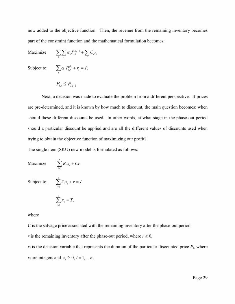
now added to the objective function. Then, the revenue from the remaining inventory becomes
part of the constraint function and the mathematical formulation becomes:
Maximize
i t iiitii rCP i 1
,
Subject to: it
itii IrP i ,
1,, titi PP
Next, a decision was made to evaluate the problem from a different perspective. If prices
are pre-determined, and it is known by how much to discount, the main question becomes: when
should these different discounts be used. In other words, at what stage in the phase-out period
should a particular discount be applied and are all the different values of discounts used when
trying to obtain the objective function of maximizing our profit?
The single item (SKU) new model is formulated as follows:
Maximize
n
iii CrxR
1
Subject to: IrxVn
iii
1
,1
Txn
ii
where
C is the salvage price associated with the remaining inventory after the phase-out period,
r is the remaining inventory after the phase-out period, where r ≥ 0,
xi is the decision variable that represents the duration of the particular discounted price Pi, where
xi are integers and ,0ix ni ,...,1 ,

Page 30
Pi is discounted price throughout the different phase-out periods (using the policy of the firm
under study, Pi is decreasing throughout the phase-out period in a constant pre-determined
manner, where: CPPP n ...21 ).
ii PV is the volume associated price Pi in a period, where nVVV ...21 due to α > 0 and β
< -1, and
1 ii PR is the revenue associated price Pi in a period, where nRRR ...21 .
3.2 Deliverables to the Return Products model
As of 2000, product returns averaged approximately 6% of sales (Stock, 2001). The rate
of product returns is usually higher for books, magazines, apparel, greeting cards, CD-ROMs and
electronics. In particular, mail catalogue or on-line sales are more vulnerable to product returns.
Typical reasons for product returns may include: defects, in transit damage, trade-ins, product
upgrades, and exchanges for other products, refunds, repair, recalls, and order errors. In this
dissertation, the focus is on the products that are getting returned due to the phase-out process by
the distributor. Regardless of the reasons for the returns, firms either absorb the cost of return
shipment or offer a money back guarantee for returned products, making product returns a major
cost center. To control the cost of handling returns, a growing number of firms and their third
party logistics providers have begun to examine ways to improve the efficiency of product
returns. Examples of such ways are: (1) the reduction of return shipping costs by taking
advantage of economies of scale. A number of separate consolidation points such as centralized
return centers can be established to aggregate small shipments into a large shipment, (2) the
enhancement of customer convenience for product returns. A number of initial collection points

Page 31
near to the customer population center can help customers reduce their travel time to the
collection points for returns, and (3) the reduction in transit inventory carrying costs associated
with product returns. Since in transit inventory carrying costs are proportionately related to
transit time of transportation modes that are used for return shipment, one should consider the
fastest mode of transportation while weighing its freight rate.
Although many customers prefer to return computers directly to original equipment
manufacturers (OEMs), direct shipment is far more costly than indirect shipment due to frequent,
small volume shipment that often requires a premium mode of transportation. In addition, many
customers do not want to deal with the hassle of making shipping arrangements for returns
through regional postal services. Even though these collection points will not incur fixed costs
such as land purchase, lease, and property tax, they will however incur variable costs associated
with renting limited space designated for the non selling returned products. Given the limited
storage space of the initial collection points, returned products at the collection points should be
quickly transshipped to centralized return centers where returned products are inspected for
quality failure, sorted for potential repair or refurbishment, stored long enough to create volume
for freight consolidation, and shipped to original manufacturers. From centralized return centers,
some returned products, which are found to be defect or damage free, may be re-distributed to
customers after repackaging or re-labeling. Centralized return centers are dedicated to return
handling and processing. On the other hand, centralized return centers may play a critical role in
linking the initial collection points to manufacturing or repair facilities within the reverse
logistics network. One can bypass the centralized return center for returning products to
manufacturers, if the initial collection points are closer to the location of given manufacturers
than that of centralized return centers since consolidation at the centralized return center

Page 32
considerably delays the return process. With the above situations in mind, the main issues to be
addressed are:
1. Location of initial collection points (ICP) in such ways that travel time (or distance)
from existing and potential customers to the collection points is minimized.
2. Location of centralized return centers (CRC) in such a way that costs of
transshipment between the initial collection points and the centralized return centers
are minimized, while freight consolidation opportunities are maximized.
3. How to build the reverse logistics network in such a way that the collection period is
minimized.
4. How many initial collection points and centralized return centers are needed to
minimize the customer hassles associated with product returns while minimizing the
costs of handling returns?
Prior to developing a model that built upon the nonlinear-mixed integer model developed
by Min et al. (2006a) described above and transforming it to a linear form, the following
assumptions and simplifications are stated: (1) the possibility of direct shipment from customers
to a centralized return center is ruled out due to insufficient volume; (2) given a small volume of
individual returns from customers, an initial collection point has sufficient capacity to hold
returned products during the collection period; (3) the transportation costs between customers
and their nearest collection points are negligible given short distances between the two parties;
(4) the location/allocation plan covers a planning horizon in which no substantial changes are
incurred in customer demands and in the transportation infrastructure, and (5) all customer
locations are known and fixed a priori.

Page 33
The model is used for the return of the remaining inventory to the manufacturer or
distributor by going through initial collection points. The ultimate goal was to minimize the total
reverse logistics costs associated with this process, which are comprised of five annual cost
components: the cost of renting the initial collection points, the handling costs at those points,
the cost of establishing and maintaining the centralized return centers, the inventory carrying
cost, and most importantly, the transportation cost.
After the linearization of the problem, closed form solutions are offered for specific cases
where a relationship between the collection period and the transportation cost is found.
3.3 Research Objectives
The following is a brief description of all the objectives to be accomplished from the
mentioned above models. Considering a particular product that is being discontinued in a retail
store, design models are developed to (1) deplete the initial inventory; (2) determine the prices
for the different time periods throughout the phase-out period; (3) determine when and for how
long to implement the markdown prices; (4) determine the optimal collection period for the
remaining inventory; and (5) maximize the total revenue of the whole process.

Page 34
Chapter 4
Solution Methodology
This chapter presents the solution methodology which includes the models, the
assumptions, and the results, for all the different models proposed in the previous chapter,
pertaining to the phase-out case, as well as to the reverse logistics aspect of the dissertation.
During this process, the key issues are addressed and the necessary suitable steps are undertaken.
4.1 Solution to the Phase-out models
This section will focus on the phase-out problem, including its multi-faceted dimensions.
The problem involves a particular product at the end of its life, after a decision has been made to
phase it out within a fixed time period. Starting with an initial inventory, the model designed to
determine the best prices to use during the different periods to maximize revenue. The data for
the total units sold and the total volume were provided by a U.S. retailer for a 54 week period.
To obtain better results, a clustering analysis of the data has been adopted to facilitate a better
understanding of the behavior of demand with respect to changes in price. The most effective
clustering method was based on calculating averages of prices and narrowing down the set of
data from a 54 point set to an approximate 9 point set, where each average of price represents the
cluster of prices around that particular price. That method is also known as the k-means
algorithm where the steps include, choosing the number of clusters, k, then randomly generate

Page 35
those k clusters and determine the cluster centers, or directly generate k random points as cluster
centers. The next step is to assign each point to the nearest cluster center, where "nearest" is
defined with respect to one of the distance measures discussed in the previous chapter, re-
compute the new cluster centers, and repeat the two previous steps until a convergence criterion
is met.
The next major step is to find which of the regression models provides the best fit to
relate the demand to the changes in price. Simple linear regression analysis was the initial type
of regression to be considered: y = a + bx, where y is the total sales volume dependent variable,
and x is the unit price independent variable. The coefficients ),( ba can be calculated by solving
the following normal equations for polynomial regression:
xbkay
2xbxaxy
The power regression approach was analyzed next to see if a better fit to the data can be
obtained:
baxy , where
2
11
2
1 11
ln)(ln
lnln))(ln(ln
n
ii
n
ii
n
i
n
ii
n
iiii
yxn
yxyxnb ,
n
xbye
n
i
n
iii
a
1 1
)(ln)(ln
The same procedure was implemented for all multiple items of the same product and it was
found that the power regression formula was similar to the price elasticity of demand equation.
After implementing the clustering procedure, the newly obtained reduced number of data sets
was used as the phase-out period, where every point represents a period. The following is the

Page 36
model developed with aim to maximize the revenue based on determining what would be the
best prices for each period during the entire phase-out process:
Maximize
T
ttP
1
1,11
1 (4.1)
Subject to: ,11
,111 IP
T
tt
(4.2)
where (t = 1, 2 …, T) are the different time periods and I1 is the initial inventory to be depleted.
Lagrangean multipliers were used to obtain a solution to the model. Let λ1 ≥ 0 be the
Lagrangean multiplier to the single constraint above. Then, the Lagrangean function is
)),...,,((),...,,(),,...,,( 1,12,11,11,12,11,1,12,11,1 IPPPgPPPfPPPL TTT
)....(... 1,112,111,1111
,111
2,111
1,11111111 IPPPPPP TT
By setting 0
tP
L, t = 1, 2 …, T and 0
L
, the following is obtained
0)1( 1,1111,111
,1
11 ttt
PPdP
dL
(4.3)
for t = 1, …, T
and .0... 1,112,111,111
111 IPPPd
dLT
(4.4)
The solution of the system of the above two equations (4.3) and (4.4), is:
1...
1
11,12,11,1
TPPP . (4.5)
Replacing this result in equation (4.4), the following results are obtained:
1/1
1
1,12,11,1 ...
T
IPPP T (4.6)

Page 37
and
1
1
1
/11
1
1
)(
)(
T
IRMax
. (4.7)
For a particular SKU (n) and a particular number of periods / prices (T): n
n
nTn T
IP
/1
,
,
where ni ,...,1 and Tt ,...,1
T
t
n
i ii
iMax
i
i
i
t
IR
1 1/1
1
)(
)(
(4.8)
To ensure that the stationary solutions attained above would result in the maximum revenue,
further analysis of the model was conducted, by using the Lagrangean method.
The Lagrangean function for the nonlinear optimization problem {max f(X) | g(X) = 0} is
defined as )()(),( XgXfXL
The equations, 0X
Land 0
L
, yield the necessary conditions, given above, and hence the
Lagrangean function can be used directly to generate the necessary conditions.
Define )()(
|
|0
nmnmT
B
QP
PH
where
nmm Xg
Xg
P
)(
)(1
andnnji xx
XLQ
),(2 , for all i and j.
In this case, there is only one constraint g(X).
Simplifying the model to two periods:
12
11
2
1
1
PPPt
t
Subject to the constraint:

Page 38
IPt
t
2
1
.
As shown above, 21 1PP
and
/1
21 2
IPP ,
/1
2
1
I
The matrix HB is identified as the bordered Hessian matrix. Given the stationary point ),( 00 X
for the Lagrangean function and the bordered Hessian matrix evaluated at that point, then X0 is a
maximum point if, starting with the principal major determinant of order (2m + 1), and the last
(n – m) principal minor determinants of HB form an alternating sign pattern starting at 1)1( m .
])2/)(1([)1(0)(
0])2/)(1([)1()(
)()(0
/12
22
12
/11
21
11
12
11
IPPP
IPPP
PP
H B
The principal minor determinant is of order (2m + 1) = 3, since m = 1. The last (n – m) principal
determinant is equal to 1 since n = 2, which forms an alternating sign pattern starting at (-1) m+1 =
1. In order for these prices to yield the maximum revenue, the last T - 1 principal minor
determinants of the Bordered Hessian matrix must have an alternating sign pattern starting at (+)
with the principal minor determinant of order 3. The principal minor determinant of order k + 2,
k = 1, 2 …, T - 1, is
1
1
1
11
1
222 )1(
k
tt
k
tt
kkk PPM
, and it has an alternating pattern starting at (+)
with 3M because β < -1.
To prove that IPP 21 defines a convex set, it suffices to prove that
21212121 )1()1())1(())1(( yyxxyyxx

Page 39
for any 0 ≤ λ≤ 1. (x1, y1) and (x2, y2) are two points in the convex set, i.e., the coordinates of
each point are associated with P1 and P2.
The right hand side of the inequality is less than I/α (Initial volume to be depleted / coefficient of
the power function of the Volume as a function of price):
I
yyxx 2121 )1()1( .
This is proven by using the constraints to the objective function for two random points in the
convex set: Iyx 11 and ,22 Iyx and then adding the two equations together after
multiplying the first constraint by λ and the second by (1-λ), respectively.
Assuming that 1 and 1,,, 2121 yyxx ,
121 ))1(( xxx and/or 221 )1())1(( xxx
121 ))1(( xxx and/or 221 )1())1(( xxx
2121 )1())1(( xxxx .
By the same deduction, .)1())1(( 2121 yyyy
Adding the above two inequalities results in,
.)1()1())1(())1(( 21212121 yyxxyyxx
Therefore, for ,10
.)1()1())1(())1(( 11112121 yyxxyyxx
This signifies that every point (price) on the line segment defined by the two analyzed above
points is also within the set.
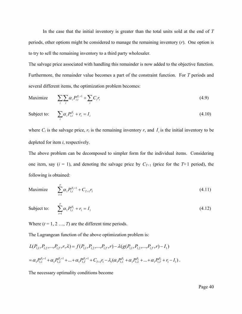
Page 40
In the case that the initial inventory is greater than the total units sold at the end of T
periods, other options might be considered to manage the remaining inventory (r). One option is
to try to sell the remaining inventory to a third party wholesaler.
The salvage price associated with handling this remainder is now added to the objective function.
Furthermore, the remainder value becomes a part of the constraint function. For T periods and
several different items, the optimization problem becomes:
Maximize
i t iiitii rCP i 1
, (4.9)
Subject to: it
itii IrP i , (4.10)
where Ci is the salvage price, ri is the remaining inventory r, and iI is the initial inventory to be
depleted for item i, respectively.
The above problem can be decomposed to simpler form for the individual items. Considering
one item, say (i = 1), and denoting the salvage price by CT+1 (price for the T+1 period), the
following is obtained:
Maximize
T
tTt rCP
111
1,11
1 (4.11)
Subject to: 111
,111 IrP
T
tt
(4.12)
Where (t = 1, 2 …, T) are the different time periods.
The Lagrangean function of the above optimization problem is:
)),,...,,((),,...,,(),,,...,,( 1,12,11,1,12,11,1,12,11,1 IrPPPgrPPPfrPPPL TTT
)...(... 11,112,111,111111
,111
2,111
1,11111111 IrPPPrCPPP TTT
.
The necessary optimality conditions become

Page 41
,0)1( 1,1111,111
,1
11 ttt
PPdP
dL
(4.13)
for t = 1, …, T
0111
TCdr
dL, (4.14)
and 0... 11,112,111,111
111 IrPPPd
dLT
. (4.15)
Solving equation (4.14), the following result is obtained: .11 TC
Furthermore, solving system of equations (4.13) simultaneously yields
11...
1
11
1
11,12,11,1
T
T
CPPP and .
1
1
1
11111
TCTIr
Since r1 needs to be non-negative, imposing r1 ≥ 0 above implies that
1
11
1111
TCTI .
11/1
1
1
1
11
T
ICT
This is a remarkable result because it provides the minimum salvage price above of which it is
better for the company to leave inventory at the end of the phase-out period. Thus, it would be
more beneficial not to lower the prices further but instead selling the remaining inventory (r1) to
a third party wholesaler.
The above mentioned results were verified using Lingo. How much to sell, how much
remains, and the price by which to sell the item during the phase-out period, can all be
determined if the following factors are known: (1) the duration of the phase-out period; (2) the
“alpha” and “beta” from the cluster analysis power regression model; and (3) the initial volume
to be depleted.

Page 42
There are many different types of nonlinear programming problems, depending on the
characteristics of the objective function f(x) and the constraint functions gi(x). Different
algorithms are used for the different types. The general constrained problem uses the Karush-
Kuhn-Tucker (KKT) conditions for optimality. Assume that f(x), g1(x), g2(x), …, gm(x) are
differentiable functions, then ),...,,( 21 nxxxx can be an optimal solution for the nonlinear
programming problem only if there exist m numbers m ,...,, 21 such that all the following KKT
conditions are satisfied:
1. 01
m
i j
ii
j x
g
x
f
2. 01
m
i j
ii
jj x
g
x
fx At x = x*, for j = 1, 2… n.
3. 0)( ii bxg
4. 0))(( iii bxg For i = 1, 2…m.
5. 0jx For j = 1, 2…n.
6. 0i For i = 1, 2…m.
Applying these conditions to our model, the following is considered:
Maximize CrPT
tt
1
1
Subject to: IrPT
tt
1
And 0r , 0tP where: t = 1 … T
An equivalent form with all constraints being “≤ 0” is:

Page 43
Maximize CrPT
tt
1
1 (4.16)
Subject to: IrPT
tt
1
(4.17)
0 tP , t = 1 … T (4.18)
0 r (4.19)
Let u, vt (t = 1 … T) and w be the Lagrangean multipliers associated with constraints (4.17),
(4.18) and (4.19), respectively. The KKT necessary conditions for optimality at
),,...,,...,( 1 rPPP Tt are:
0)1( 1 ttt vPuP , t = 1 … T (4.20)
C – u + w = 0, u ≥ 0, w ≥ 0, vt ≥ 0, t = 1 … T (4.21)
01
IrPuT
tt (4.22)
0tt vP (4.23)
0rw (4.24)
IrPT
tt
1
(4.25)
0tP , t = 1 … T (4.26)
0r (4.27)
Constraints (4.20) and (4.21) are the optimality conditions, constraints (4.22) – (4.24) are the
complementary slackness conditions, and constraints (4.25) – (4.27) are the feasibility
conditions.

Page 44
It is assumed that u = 0. Then (4.20) and (4.26) imply that 0)1( tt Pv for t = 1 … T,
since β < -1. This contradicts (4.21). Furthermore, for 0tP , t = 1 … T, the
tP
Pt 0
lim , and
constraint (4.25) is violated. Therefore u > 0 and (4.22) implies:
IrPT
tt
1
(4.28)
In addition, 0tP , t = 1 … T, which implies from (4.23) that vt = 0, t = 1 … T and (4.20) yields
uPt
1
, t = 1 … T.
Finally, r can be positive or zero. If r > 0, then w = 0, and (4.21) implies that u = C. Therefore,
CPt
1
, t = 1 … T and (4.28) yields
T
t
CIr1 1
.
If r = 0, (4.28) yields
/1
T
IPt , t = 1 … T and u becomes:
/1
11
T
IPu t
In addition, since r = 0, (4.24) implies that w ≥ 0, and combining that with (4.21), w = u – C ≥ 0
is obtained. Substituting u from above, results in the following inequality for C:
/1
1
T
IC .
The following theorem and corollary follow the above KKT conditions derivation.
Theorem 1. The optimal solution of the maximizing revenue problem with an initial inventory to
be depleted over a finite time horizon, where the demand is a nonlinear function of price is

Page 45
solved by finding the optimal price for every period t, CPt
1
, t = 1 … T and the
remaining inventory,
T
t
CIr1 1
.
Corollary 1. If the salvage price is lower than a certain threshold,
/1
1
T
IC then
items should not be left at the end of the time horizon T.
The single period process was used for a dynamic pricing policy, where the model ran for
the first period, and the remaining inventory was used at the end of that period as the new initial
inventory for the new period. The same process was repeated until the end of the phase-out
period. By updating the inventory at the beginning of every period, it was found that the prices
remain the same throughout the phase-out periods. In addition, the resulting values are exactly
the same as the prices obtained, when the model ran for the entire phase-out period as a whole.
4.2 Solution to the Return Products model
Moving forward from the results of the previous section, if it was decided to consider
returning the remaining inventory to the manufacturer or the distributor, there is a need to
implement a reverse logistics model to help minimize all the costs associated with this operation,
such as the renting and handling costs at the initial collection points, establishing and
maintaining the centralized return centers, inventory carrying costs, and transportation costs.
Some of the decisions to be made are which initial collection points and centralized return
centers to be established, which customer is allocated to which initial collection point, and the
volume of products to be returned from an initial collection point to a centralized return center.

Page 46
In addition, freight discount rates based on quantity and distance should be explicitly considered.
The complete mathematical model is presented next with symbol definitions and mathematical
formulation.
Indices:
i = index for customers; Ii
j = index for initial collection points; Jj
k = index for centralized return centers; Kk
Decision Variables:
jkX = volume of products returned from initial collection point j to centralized return center k
if customer i is allocated to initial collection point j otherwise if an initial collection point is established at site j otherwise
T = length of a collection period (in days) at each initial collection point
if a centralized return center is established at site k )( Kk otherwise
Model Parameters:
aj = annual cost of renting initial collection point j
b = daily inventory carrying cost per unit
w = annual working days
ri = volume of products returned by customer i per day
hj = handling cost of unit product at initial collection point j
,0
,1ijY
,0
,1jZ
,0
,1kG

Page 47
ck = annual cost of establishing and maintaining centralized return center k
mk = maximum processing capacity of centralized return center k in new returns per day
dij = distance from customer i to initial collection point j
djk = distance from collection point j to centralized return center k
l = maximum allowable distance from a given customer to an initial collection point
T = maximum length of a collection period (in days) at an ICP. This upper bound on the length
of collection days is necessary to assure that return lead time is not too long for the customers
Ci = }|{ ldj ij set of initial collection points that are within distance l from customer i
Dj = }|{ ldi ij set of customers that are within distance l from initial collection point j
jkjkjkjk EdXf ),( unit transportation cost between collection point j and return center k
where E is the standard freight rate ($/unit), jk is the freight discount rate according to the
volume of shipment between initial collection point j and centralized return center k, and jk is
the penalty rate applied for the distance between initial collection point j and centralized return
center k.
22
211
11
PXfor
PXPfor
PXfor
jk
jk
jk
jk
22
211
11
Qdfor
QdQfor
Qdfor
jk
jk
jk
jk
Figure 9 shows the benefits from the economies of scale (i.e., freight discounts) and/or penalties
due to distance for a certain shipment jkX between ICP j and CRC k that are jkd distance away.
Although only two breakpoints are specified for volume shipment (P1 and P2) and distance (Q1

Page 48
and Q2), any number of points can be accommodated by the proposed model which can mimic
class rates in practice.
Mathematical Formulation:
Minimize
Kk
jkjkJj
jkKk
kkIi Cj
ijjiIi
iJj
jj dXfXT
wGcYhrwr
TbwZa
i
),(2
1 (4.29)
Subject to
1 iCj
ijY Ii (4.30)
jDi
jij ZMY Jj (4.31)
k
jkDi
iji XYrTj
Jj (4.32)
kkj
jk GTmX Kk (4.33)
djk
Xjk
E
Eα1 Eα2
Eα1β1
Eα2β1 Eβ1
Eα1β2
Eß2 Eα2β2
Q1
Q2
P1
P2
Figure 9: Unit transportation cost function

Page 49
,0jkX Jj Kk (4.34)
}1,0{ijY Ii Jj (4.35)
}1,0{jZ Jj (4.36)
}1,0{kG Kk (4.37)
The objective function (4.29) minimizes the total reverse logistics costs, which are
comprised of five annual cost components: the cost of renting the ICPs, the cost of establishing
and maintaining the CRCs, the handling costs at the ICPs, the inventory carrying cost, and the
transportation cost.
Constraint (4.30) assures that a customer is assigned to a single initial collection point.
Constraint (4.31) prevents any return flows from customers to be collected at a closed ICP (M is
an arbitrarily set big number). Constraint (4.32) makes the incoming flow equal to the outgoing
flow at each initial collection point. Constraint (4.33) ensures that the total volume of products
shipped from initial collection points to a centralized return center does not exceed the maximum
capacity of the centralized return center. Constraint (4.34) preserves the non-negativity of
decision variables jkX . Constraint sets (4.35) – (4.37) declare decision variables ijY , jZ and kG
as binary.
4.2.1 Linearization of the Model
The first contribution is to linearize the model. The non-linearity of the last term of the
objective function
Kkjkjk
Jjjk dXfX
T
w),( can be transformed to a linear term ),( jkjkjk dXfX
as follows:

Page 50
For any given (j,k) pair, jk can be easily determined by the known value of jkd . Parameter jk ,
however, depends on the value of decision variable jkX and therefore cannot be determined in
advance. The following transformation is used to linearize the term ),( jkjkjk dXfX . Let 1jkU ,
2jkU and 3
jkU be continuous variables associated with ranges ],0[ 1P , ],( 21 PP and ),( 2 P ,
respectively, such that
321jkjkjkjk UUUX (4.38)
and
101
11
12
22
3
P
UW
PP
UW
M
U jkjk
jkjk
jk , (4.39)
where 1jkW and 2
jkW are binary variables and M is a big number. Accordingly, when 1jkW = 2
jkW =
0, then 11 PUX jkjk
is in the first range; when 1
jkW = 1 and 2jkW = 0, then 1
1 PU jk ,
122 PPU jk , 3
jkU = 0 and jkX is in the second range. Finally, when both Wjk’s take the value
of 1, then jkX is in the third range (See Figure 10). The term ),( jkjkjk dXfX can now be
mathematically expressed as a linear function of Ujk’s and Wjk’s:
,)()(),( 22
323311
212211jkjkjkjkjkjkjkjkjkjkjkjkjkjkjk WPrrUrWPrrUrUrdXfX
where jkjk Er 1 , jkjk Er 12 and jkjk Er 2
3 are the slopes of function ),( jkjkjk dXfX , as
shown in Figure 10:
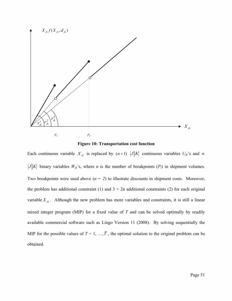
Page 51
),( jkjkjk dXfX
jkX
P1 P2
Figure 10: Transportation cost function
Each continuous variable jkX is replaced by )1( n KJ continuous variables Ujk’s and n
KJ binary variables Wjk’s, where n is the number of breakpoints (Pl) in shipment volumes.
Two breakpoints were used above (n = 2) to illustrate discounts in shipment costs. Moreover,
the problem has additional constraint (1) and 3 + 2n additional constraints (2) for each original
variable jkX . Although the new problem has more variables and constraints, it is still a linear
mixed integer program (MIP) for a fixed value of T and can be solved optimally by readily
available commercial software such as Lingo Version 11 (2008). By solving sequentially the
MIP for the possible values of T = 1, …,T , the optimal solution to the original problem can be
obtained.
1jkr
2jkr
3jkr

Page 52
Chapter 5
Special Problem Structures
This chapter presents the special structures of the models discussed earlier in Chapter 4,
and further dissects the solutions obtained in order to handle the specific cases where theorems
and corollaries are derived. This work aims to set the foundation for the next chapter where the
computational results are detailed and sensitivity analysis performed. During this process, the
following section will discuss the different issues that were encountered during research, along
with the steps taken to resolve them. In summary, this chapter will present the assumptions made
for the special structures and the closed form solutions.
5.1 Markdown Strategies Analysis
A special case arises in the phase-out problem, where the prices are pre-determined, i.e.,
it is known by how much to discount; therefore, the main question becomes: when these different
discounts should be applied and for how long? In addition, should all the different discounts be
used or not when trying maximize revenue?
The mathematical model for this case can be formulated as follows.
Maximize
n
iii CrxR
1
(5.1)
Subject to: IrxVn
iii
1
(5.2)

Page 53
n
ii Tx
1
(5.3)
where C is the salvage price associated with the remaining inventory after the phase-out period.
r is the remaining inventory after the phase-out period, where r ≥ 0
xi is the decision variable that represents the duration of the particular discounted price Pi, where
xi are integers and ,0ix ni ,...,1 .
Pi is the ith. Using the policy of the firm under study, Pi is decreasing throughout the phase-out
time horizon in a constant pre-determined manner, i.e., ....21 CPPP n
ii PV is the volume sold in one time period when discounted price Pi is applied. It follows
that nVVV ...21 due to α > 0 and β < -1.
1 ii PR is the revenue in one time period associated with discounted price Pi. It follows from
above that nRRR ...21 .
The problem defined above by equations (5.1) – (5.3), can be readily solved by MIP
software such as Lingo (2008). However, since the number of constraints is only two, the aim is
to find a closed form solution of the linear version of the problem, i.e., considering xi to be
continuous variables. The xi values can then be rounded to the closest integer to obtain an
appropriate solution. Given that there are only two constraints in the resulting linear
programming problem, there will be only two basic variables in the optimal solution. This will
result in two cases:

Page 54
Case 1: r and xj are the two basic variables
This set of equations can be denoted by bBxB where the vector of basic variables
r
xx j
B ,
the basis matrix
01
1jVB , and
T
Ib . Therefore, the desired solution for the basic variables
is 01
101
Tx
T
I
Vr
xbBx j
j
jB and
T
IVTVIr jj 0
Applying the optimality test on the reduced costs of the non-basic variables, the following is
obtained:
jjiiijjiii
jj CVRCVRRCVRCVR
V
VCR
0011
10][ .
The solution is guaranteed ifT
IV j , which means that if jV
T
I for all },...,1{ nj , an infeasible
solution results. This infeasibility is due to a lack of enough amount of inventory in this case.
Case 2: xj and xk are the two basic variables
Using the same notation for the set of equations, bBxB , the vector of basic variables now
becomes
k
jB x
xx , the basis matrix
11kj VV
B , and
T
Ib . Therefore, the solution for the
basic variables is
01
1
1
kj
kj
kj
j
kj
kj
k
kj
k
jB VV
TVIx
T
I
VV
V
VV
VV
V
VV
x
xbBx and 0
kj
jk VV
TVIx .
Without loss of generality, let it be assumed that kj VV .

Page 55
Then kk VT
ITVI 0 and
T
IVTVI jj 0 . Therefore, kj V
T
IV .
Again, consistent with the previous case, if there does not exist a j such thatT
IV j , there is no
feasible solution.
If kVT
I , for all },...,1{ nk , then this is the case of excessive inventory, and it would be
impossible to deplete all of it, by discounted prices; as a result, there will always be remaining
inventory at the end of the phase-out period.
Applying the optimality test on the reduced costs of the non-basic variables, the following is
obtained:
011
1
][
i
i
kj
j
kj
kj
k
kjkj R
V
VV
V
VV
VV
V
VVRR .
Again, without loss of generality, assuming that kj VV , implies
00
kj
kjjk
kj
ikiji
kj
kjjk
kj
ikij
VV
VRVR
VV
VRVRR
VV
VRVR
VV
VRVR
jk
jkkjikjjkikij RR
VRVRVVRVRVRVR
0
And j
kj
kj
kj
j
kj
kj
k
kjkj C
VV
RRC
VV
V
VV
VV
V
VVRR 00
0
1
1
1
][
kj
kj
VV
RRC

Page 56
Based on this optimality condition, the objective was to prove that jV and kV represent the
volume of two consecutive prices, respectively, and that any value iV will either fall below jV or
above kV . Consider any three consecutive prices, say 321 ,, PPP . It is sufficient to show that the
following lemma holds.
Lemma 1. For 321 PPP , where ii PV , 1 ii PR , i = 1, 2, 3, and 1 , the
incremental rate of return is decreasing with i , or .023
23
12
12
VV
RR
VV
RR
Proof. Let
1 . Since β < -1 01 and 0
1
Furthermore, .11
1
Therefore, for β < -1 , 0 < γ < 1.
Consider the transformation ii PY , i = 1, 2, 3. Since 321 PPP , 321 YYY .
Substituting γ for β and using the transformation, the inequality 023
23
12
12
VV
RR
VV
RRbecomes
023
23
12
12
YY
YY
YY
YY
, which holds because Y is a concave function of Y (γ is a constant).
The results from this optimality condition along with the model and its constraints (after being
converted to “≤”), fit into the well known linear multiple choice knapsack problem (LMCK).
This problem has been widely investigated (Lin, 1998) and (Kozanidis et al., 2002 & 2004).
However, what makes this a unique situation is the absence of dominated variables, i.e., all the
points (Vi, Ri), when connected, form a piecewise linear concave function and are part of the non-
dominated frontier illustrated in Figure 11. The data and results used to obtain this figure will be
shown in chapter 6.

Page 57
Figure 11: Rate of change of revenue with respect to change in volume
In addition to fit into the LMCK problem, the conversion of equality constraints (5.2) and
(5.3) to “≤” type, eliminates the earlier mentioned infeasibilities and generalizes the model for
any inventory value, even small enough that may be sold in a fraction of the phase-out period T.
In summary, knowing the initial inventory “I” to be depleted, the phase-out period “T” to
deplete it by, and the different discount prices, the following algorithm provides the discount
prices to use and for how long (xi) as well as the remaining inventory to sell at salvage price so
that revenue is maximized.
Algorithm 1.
Step 1. Computeii
iii VV
RRs
1
1 , i = 1, …, n-1 (rate of change of the revenue with respect to the
change in volume). Let kT
IVV ii
i }|{maxarg and jCss ii
i }|{maxarg .
Step 2. If k = 0, set ;1
1 V
Ix ,0ix 1,1 TVIri ,
10000
11000
12000
13000
14000
15000
16000
17000
1000 1500 2000 2500 3000 3500 4000 4500
Revenue (Ri)
Volume (Vi)
Volume to Revenue relationship

Page 58
else if kj 1 , set ;Tx j ,0ix jTVIrji , ,
else, set ;1 kk
kk VV
TVIx
;1
11
kk
kk VV
ITVx
,0ix 0;1, rkki .
End if
Experimental results in the next chapter were obtained through lingo and MS Excel that
verified the accuracy of the above algorithm.
5.2 Determining the Optimal Collection Period in the
Reverse Logistics model
The optimal collection period can be analytically determined by focusing on the two
major cost components of the model, which depend on the collection period T: inventory
carrying cost and transportation cost. To simplify the analysis, it is assumed that there is no
penalty imposed on the travel distance between the ICPs and the CRCs. Equivalently, the
penalty rate has already been included into the volume discount rate, αjk, for shipments between
ICP j and CRC k. The more general case can be considered when there are n breakpoints for
freight volume discounts, P1, P2, …, Pn (see Figure 11).

Page 59
The inventory carrying cost is a linear function of the number of collection days (T) at the
ICPs,
Iiir
Tbw
2
1. Therefore, as T increases, the inventory carrying cost difference (slope) is
kept constant at
Iiir
bw
2. The transportation cost, on the other hand, is a function of the
volume of products shipped from the ICPs to the CRCs, which in turn depends on the daily
volume returned from customers to the ICPs and the number of collection days, T. Moreover,
depending on the quantity returned from a particular ICP to a CRC, a discount rate may be
applied.
Substituting ),( jkjk dXf for jkE in the transportation cost component of the objective
function (1), multiplying by Ii
irT and dividing by its equal,),( kj
jkX , results in the following
expression that provides an intuitive interpretation of shipping costs:
IiiT
Iii
kjjk
kjjkjk
kjjkjk
kjjk
Iii
rwWArwX
XE
XET
w
X
rT)(
)(
)(
,
,
,,
In other words, the annual transportation cost can be expressed as the annual number of returned
products multiplied by the effective unit transportation cost, TWA)( , which is the weighted
djk
E
Eα1
Eα2
P1
P2
…… Eαn
Pn
P0 = 0
Figure 12: Simplified unit transportation cost function

Page 60
average of the unit transportation costs ( jkE ). The weights are the shipment volumes jkX . It is
worth noting that although T was cancelled above, TWA)( depends on T through jkX and
eventually jk . In particular, TWA)( is a non-increasing function of T, since larger shipments
jkX cannot increase the unit transportation cost but they may decrease it whenever jkX moves to
a new range of consecutive discount breakpoints.
For two consecutive integer values of T, the difference between the corresponding
transportation costs is )]()()[( 1
Ii
iTT rwWAWA . This indicates that in order to determine the
change in the combined cost, as the collection period increases by one day, it is sufficient to
compare the constant slope of the change in inventory cost noted earlier,
Iiir
bw
2, to the above
non- positive change in the weighted average of the transportation cost.
5.2.1 Special Structures of the Optimal Collection Period Problem
This section addresses specific scenarios in the reverse logistics model of the dissertation
by considering the following: multiple customers are returning products to multiple ICPs and
thereafter, products are shipped to multiple CRCs; however, customers are divided into groups
(clusters) where each cluster is within the geographical area of a single ICP. In addition, no
capacity is imposed on the CRCs and fixed costs at the ICPs and CRCs are considered
negligible.
Equivalently, it may be assumed that customers have already been assigned to ICPs and
ICPs have been assigned to CRCs. The only decision to be made is to determine the number of
collection days at each ICP. Under the above scenario, the problem can be decomposed into

Page 61
smaller sub-problems, each one involving an individual cluster of customers with one ICP and
one CRC. This special structure of a reverse logistics problem for product returns allows a
closed form solution for the optimal collection period T to be found. For notational simplicity,
the total daily volume of product returns from all customers assigned to an ICP ),(Ii
ir will be
denoted by R.
A Discrete Time Collection Period Model
If the total daily volume of product returns is greater than the largest shipping volume
breakpoint, nPR , then the slope of the transportation function is nE and the optimal collection
period is T = 1. If the total daily volume of product returns R falls between two shipping volume
breakpoints, i.e. ll PRP 1 for l = 1, …, n, then the transportation cost will always decrease
with an increase in the collection period that will move the shipping volume beyond Pl, realizing
more shipping economies of scale. If a change in the transportation cost in absolute value is
larger than the change in inventory carrying cost, then the total cost will decrease from time
period T to time period T+1. The weighted average of the unit transportation cost becomes less
effective as it moves from one quadrant to the other (Figure 11).
Without loss of generality, the total daily return rate R is less than the first shipping
volume breakpoint 10 PR . The following analysis for determining the optimal collection
period can be applied for any nPR . The minimum length of the collection period T is one. At
1T , the weighted average is equal to E, the transportation cost is EwR and the inventory
carrying cost isbwR . The first time the economies of scale are implemented is at ]/[ 1 RP , where
[.] is the ceiling function. For integer values of T such that ]/P[1 1 RT , the transportation cost

Page 62
remains unchanged at EwR while the inventory cost increases linearly with
2
1TbwR . Since
the total cost is an increasing functions of T, collection periods such that ]/P[1 1 RT are not
optimal. The next value of interest after T = 1 is ]/[ 1 RPT .
In general, the collection period at ]/[ RPT l is better than collection periods T, such that
]/[]/[ 1 RPTRP ll , l = 1, …, n – 1, and the collection period at ]/[ RPT n is better than the
ones for ]/[ RPT n because the total cost is an increasing function of T within each shipping
range, wRET
bwR l
2
1, l = 1, …, n – 1. Therefore, the following theorem holds:
Theorem 2. For the special structure of a single ICP and CRC, the optimal collection period
can be either at 1 or at ]/[ RPl , l = 1… n.
The above theorem suggests a straightforward procedure for finding the optimal collection
period by comparing the total cost at only n + 1 values of T. Experimental results indicate that
the optimal collection period often occurs in the two extreme candidate values of T, i.e., 1 and
]/[ RPn . The range of values of the daily collection amount R is found below.
Based on Theorem 1, the optimality condition for T = 1 is
wREwRRPb
RwbEwR ll )1]/([2
, l = 1, …, n. After simplification, the above inequality
reduces to 11
2]/[
b
ERP ll
, l = 1, …, n. Noting that ]/[ RPl
is positive integer,

Page 63
11
2]/[b
ERP ll
, l = 1, …, n and solving for R to obtain LRR , where
11
2
min,...,1
bE
PR
l
l
nlL
(5.4)
Similarly, the optimality conditions for ]/[ RPT n are
wREwRRPb
wRERwRPb
llnn )1]/([2
)1]/([2
, l = 1, …, n – 1,
and bwREwRwRERwRPb
nn )1]/([2
. These conditions reduce to URR , where UR is the
maximum value of R satisfying
11
2
]/[2]/[
bE
PR
RPb
ERP
n
n
lnl
n
(5.5)
The above analysis leads to the following corollary for locating the optimal collection period:
Corollary 2. For the special structure of a single ICP and a single CRC, the optimal collection
period is
1,...,1,]/[
,]/[
,1
nlRP
RPT
l
n
UL
U
L
RRRif
RRif
RRif
Where LR and UR are given by (12) and (13), respectively. It should be noted that if the collection
period has an upper boundT , as defined earlier, the above corollary can be adjusted by
replacing n with l , where R
PT
R
Pll 1 .

Page 64
The above corollary provides a straightforward method to check the following: (1) if the
shipping economies of scale are not applicable because the total daily volume of product returns
R is below the lower critical value ( LR ), (2) the advantage of full shipping economies of scale
can be taken because R is beyond the upper critical value ( UR ), (3) or when partial shipping
economies of scale can be used because R is between the lower and the upper critical values. A
noteworthy observation is that the two critical values depend on the breakpoints at which freight
rate discounts occur )( lP and on the ratio of the shipping savings rate over the unit inventory
carrying cost
bl1
and the analogous ratio of the relative shipping rate over the unit
inventory carrying cost
bnl
.
A Continuous Time Collection Period Model
The collection period T is now considered to be continuous in the interval [1,T ] and each
customer i returns products to a single ICP at a uniform rate ri. If Q is the shipment quantity,
then TRQ products are shipped to a single CRC during every collection period T. Let Q fall
within range of breakpoint shipment levels, say 1 ll PQP . Then T [1,T ] implies that
integer index l [ ll, ], where
R
PT
R
Pll
R
P
R
Pll
ll
ll
1
1
|
1| and 0P = 0. The total annual cost (including
inventory carrying cost and transportation cost only) is given byT
wQEbwQ l2
. After
substituting Q in terms of T, the total cost TC reduces to a piece-wise linear function of T with
constant slope, 2/bwR , and discontinuities (jumps) at :/ RPl

Page 65
wRETbwRTC l )2/( , RPTRP ll // 1 , lll
At 1T , the total cost is wREbwR l2/ . The lowest value of the total cost within each
shipping range is obtained at the leftmost point, RPT ll / , lll 1 , where ε is an
infinitesimal quantity, practically zero. Therefore, the following theorem holds:
Theorem 3. For the continuous collection period model with shipping economies of scale, the
optimal collection period occurs at either 1T , or at one of the critical collection periods lT ,
lll 1 .
As discussed earlier, the total daily volume of product returns R determines if no shipping
discounts are used (T = 1), full shipping discounts are used )(l
TT , or partial shipping
discounts are used )11,( lllTT l under the optimal policy. A similar analysis yields the
following:
Let
12
min1
bE
PR
ll
l
lllL
, and
12
,
2
maxmax11
bE
P
bE
PPR
ll
l
ll
ll
lllU
Then the following corollary holds:
Corollary 3. The optimal collection period is 1 for LRR and l
T for URR .
For UL RRR , the optimal collection period can be at lT , ,...,1 ll 1l .

Page 66
Chapter 6
Computational Results
This chapter thoroughly analyzes all the computational results attained using the
aforementioned models. A complete breakdown, along with an extensive sensitivity analysis
was conducted using multiple tools and software. These programs included Microsoft Excel,
Lingo 11, MATLAB, SPSS, Minitab, Mathematica, and AutoCAD. The results are divided into
four different sections as detailed below. This process starts by finding an optimal markdown
strategy to deplete an initial inventory and extends to the identification of the optimal collection
period of the remaining returned products.
6.1 Clustering Procedures and Regression Analysis
The first section of this chapter highlights the usefulness and the implementation of the
clustering procedure in the different levels of the process. Furthermore, regression analysis
methods were used to find the best fit of sales-price data to a demand-price function. A fitting
start is to first describe the source and the type of the data. The data are obsolete inventory items
in retail stores, such as cosmetic items in the pharmacy X, distributed by manufacturer Y. There
are over 650 SKUs in more than 6,000 stores. The total sales volume and the total sales amount
were provided for a period of 54 weeks. Therefore, there was a need to sieve through the data
and use scientific methods to break it down. The first step taken was to analyze the largest

Page 67
possible amount of SKUs and then to narrow down the selection to the ones where a “normal”
relationship between volume and demand is found. This can be accomplished by breaking down
the geographical areas based on the states where the pharmacy X stores are located, which are in
41 states. The next step was to connect the stores from the different states, which share the same
distribution centers. After careful analysis and calculation of all excess inventories within these
stores, the focus was then shifted to the individual SKUs. This process was thoroughly
conducted until the final selection of 6 SKUs. The following table shows the 6 SKUs selected
for the detailed analysis.
Table 3: Final selection of SKUs to be analyzed Pharmacy X SKU
Number ITEM DESCRIPTION
111111 LIP 555 111112 LIP 560 111113 LIP 587 111114 LIP 701 111115 LASH 830 111116 LASH 835
Next, the relationship between the total units sold and the total amount sold for 54 weeks
was analyzed for each SKU, by calculating the unit prices and drawing all different types of
comparisons between the unit prices and the units sold. Different types of regression were used,
and the power regression proved to be the best fit for all the SKUs analyzed. In addition, a
clustering algorithm was used to come up with the relevant unit prices to describe all sales. The
following is a breakdown of an example SKU and the steps involved in the process just
mentioned.

Page 68
For illustration, the last SKU in Table 3, number “111116”, is considered below. Figure
13displays a graph showing the relationship between the unit prices and the total sales volume
for the entire 54 week period.
Figure 13: Unit price vs. total sales volume for a particular SKU
As Figure 13 shows, there are very few data points for low unit prices. This was true for
other SKUs as well. It was evident therefore that there was a need to cluster the data to
determine a better understanding of the relationship between price and demand. Thus, a k-means
algorithm was used where the number of clusters k, had to be chosen first. The cluster centers in
this case are represented by the unit prices. Using k = 9, the clustered data are shown in Table 4
and Figure 14, respectively, around 9 different unit prices.
0
500
1,000
1,500
2,000
2,500
3,000
3,500
4,000
4.00 5.00 6.00 7.00 8.00 9.00 10.00
Total Sales Volume
Unit Price
SKU # 111116

Page 69
Table 4: K-means algorithm results
Cluster Means (Unit Price) Total Sales Volume 4.58 3,407 5.13 2,890 6.10 1,767 6.50 1,775 7.01 1,621 7.83 1,705 8.37 1,142 8.74 1,155 8.95 1,132
Figure 14: Cluster means (unit price) vs. total sales volume for a particular SKU
The same procedure was followed for all the SKUs under study. The next step was to try
to figure out what resulted in the best fit model. As mentioned before, the power regression
analysis showed a better fit. The power equation for SKU # 111116 is shown in Figure 14.
Demand as a function of price according to the equations obtained from the regression
analysis, fit into the family of elasticity of demand equations. Thus, the general form for the
demand function can be written asPpV )( , where P is the unit price and V is the total
sales volume. β is the price elasticity of demand constant and α is a positive constant.
y = 37625x‐1.605
R² = 0.9339
0
1,000
2,000
3,000
4,000
4.00 5.00 6.00 7.00 8.00 9.00 10.00
Total Sales Volume
Cluster Means (Unit Price)
SKU # 111116

Page 70
If 0 then V , this is the case of a perfectly inelastic condition. If 1 then PV , this
will represent the standardized form of the equation. Normalizing the equations, and using them
to see how the volume changes by systematically decreasing to 40 percent of its original price,
the behavior was observed and compared amongst all the different SKUs. Table 5 and Figure 15
below show the results.
Table 5: As Unit price decreases, volume increases SKU 111116 111115 111114 111113 111112 111111 UP ↘ TSV ↗ TSV ↗ TSV ↗ TSV ↗ TSV ↗ TSV ↗ 1.00 1.00 1.00 1.00 1.00 1.00 1.000.9 1.18 1.20 1.31 1.29 1.30 1.280.8 1.43 1.48 1.78 1.71 1.74 1.680.7 1.77 1.88 2.50 2.36 2.43 2.290.6 2.27 2.46 3.72 3.42 3.57 3.280.5 3.04 3.40 5.95 5.31 5.63 5.00
0.4 4.35 5.03 10.57 9.08 9.82 8.40
y = x^(-1.605) y = x^(-1.764) y = x^(-2.574) y = x^(-2.408) y = x^(-2.493) y = x^(-2.323)
Figure 15: Comparison of the power functions of the different SKUs
Clustering Procedures and Regressions Analysis served as the stepping stone to develop the
mathematical models and addresses the various inventory issues.
1.00
2.00
3.00
4.00
5.00
6.00
7.00
8.00
9.00
10.00
11.00
12.00
0.30 0.40 0.50 0.60 0.70 0.80 0.90 1.00
Incr
ease
by
nu
mb
er o
f ti
mes
in TSV
Decrease in Unit Price (Standardized)

Page 71
6.2 Inventory depletion and markdown strategies within a
phase-out period
This particular phase of the dissertation focuses on the results obtained from the
inventory and markdown strategy models presented in the previous chapters. The first
assumption made is that SKU # 111116 has been phased-out due to manufacturer’s decision or
due to lack of sales, and that the phase-out period is pre-determined. The second assumption is
that the phase-out period is 9 weeks. Starting with that initial inventory at the beginning of the
phase-out period, the first problem is to determine by how much to discount through every
period to completely deplete the entire initial inventory by the end of the nine weeks.
Maximizing the revenue based on the model
T
ttP
1
1 that is subject to: IPT
tt
1
Where t = 1, 2 …, T are the different time periods, “I” is the initial inventory to be depleted, and
alpha and beta are determined from the power regression analysis done in the previous section of
this chapter. For SKU # 111116, α = 37,625 and β = -1.605, and I = 20742 units.
Solving the model through Lingo, the optimal solution resulted in the same price for every time
period throughout the phase-out process. That optimal price is calculated by the following
equation: ,/1
T
IPt which will lead to maximum revenue of .
)(
)(/1
1
T
IRMax
For SKU # 111116, the price obtained for every time period is $5.70, which will result in total
revenue of $118,237. Table 6 shows a summary of the optimal prices and maximum revenues
for all 6 SKUs.

Page 72
Table 6: Optimal prices / maximum revenue at the end of the phase-out period SKU # α β Initial Inventory Optimal Price Max Revenue 111116 37625 -1.605 20,742 5.70 118,237 111115 69700 -1.764 28,726 5.75 165,043 111114 10325 -2.408 3,205 4.05 12,975 111113 16946 -2.574 3,930 4.14 16,284 111112 12941 -2.493 3,188 4.24 13,502 111111 11362 -2.323 4,058 4.01 16,279
These results are attained only in the case of a complete depletion of an initial inventory of a
particular SKU over a phase-out period given a price elasticity of demand type of function.
In the case that the initial inventory is greater than the total units sold at the end of T
periods, other options to handle the remaining inventory (r) can be considered. One option is to
attempt to sell the remaining inventory at some salvage price to a third party wholesaler. The
revenue from selling the remaining inventory is now added to the objective function.
Furthermore, the remaining inventory becomes part of the constraint function.
Objective function:
Maximize
tt CrP 1 (6.1)
Subject to: IrPt
t (6.2)
where C is the salvage price associated with the remaining inventory r for a particular SKU,
and I is the initial inventory to be depleted, and 1 tt PP , t = 2, …, n.
The solution now results in a new optimal price, which is still identical for every time period and
is calculated according to the following equation:1
C
Pt , t = 2, …, n.

Page 73
The solution demonstrates that selling the remaining inventory to a third party wholesaler is only
beneficial if the salvage price is greater than a certain value: .1
/1
T
IC
Table 7 presents the minimum values of the required salvage price for all 6 SKUs:
Table 7: Lowest values of salvage price C SKU # Minimum Salvage Price required 111116 2.15 111115 2.49 111114 2.37 111113 2.53 111112 2.54 111111 2.28
Finding the lowest value that the salvage price can take proves to be very crucial for the
retailer, since the salvage price at which the remaining inventory is sold can be determined. The
optimal price for every time period during the phase-out is a function of the salvage price, which
means that as C increases, so does P; naturally, this will also increase the maximum revenue.
However, it is not reasonable to have a salvage price higher than the actual price of the item
being sold during the phase-out period. Therefore, returning the products to the manufacturer /
distributor is the next option to evaluate in the next section of this chapter.
However, before tackling the reverse logistics model for the return products, a
mathematical model was developed, which addresses the inventory problem from a different
perspective. If the markdown prices are set in advance and they are fixed, the question becomes:
when to use them and for how many periods during the phase-out time horizon? With the initial
inventory remaining the same and the length of the phase-out period also unchanged, it was
important to resolve when to use the pre-determined markdown prices and for how long. By
revamping the model, and using the same power regression function, the following was obtained:

Page 74
Maximize
n
iii CrxR
1
(6.3)
Subject to: IrxVn
iii
1 (6.4)
Txn
ii
1
(6.5)
where, C is the salvage price associated with the remaining inventory after the phase-out period,
r is the remaining inventory after the phase-out period, where r ≥ 0,
xi is the decision variable that represents the duration of the particular discounted price Pi, where
xi are integers and ,0ix ni ,...,1 .
Pi is the discounted price throughout the different phase-out periods. Using the policy of the
firm under study, Pi is decreasing throughout the phase-out period in a constant pre-determined
manner, where: ....21 CPPP n
Considering the same SKU # 111116, Table 8 shows the pre-determined prices for the
markdown strategy:
Table 8: Pre-determined markdown prices P1 P2 P3 P4 P5 8 7 6 5 4
The two factors that determined where the solution was going to fall within the 9 week phase-out
period are the inventory / time period (I/T) ratio, and the salvage price (C), as explained in
Chapter 4.
Using the same initial inventory (I = 20742) with a total phase-out time period of 9
weeks, and with a salvage price that varies from 0 to $4, the following table shows the results of
where the solution falls, along with the maximum revenue.

Page 75
Table 9: Determining when and for how long to use the markdown prices
C x1 x2 x3 x4 x5 Remaining inventory
Maximum Revenue
4.00 9 0 0 0 0 8,712 131,087 3.00 9 0 0 0 0 8,712 122,375 2.50 0 9 0 0 0 5,837 118,928 2.00 0 0 6.71 2.29 0 0 117,937 1.50 0 0 6.71 2.29 0 0 117,937 1.00 0 0 6.71 2.29 0 0 117,937 0.50 0 0 6.71 2.29 0 0 117,937 0.00 0 0 6.71 2.29 0 0 117,937
This analysis was performed for different values of initial inventories, and for all 6 SKUs. The
optimal decision depends on the ratio I/T with regard to the total sales volume, and on the
salvage price (as shown in Chapter 4). The significance of the solution and its closed form is the
ability to predict in which periods the markdown strategy should be implemented, for how long,
and whether to keep any remaining inventory. In addition, it guarantees that the solution always
falls between two consecutive time periods. The following Table 10 depicts model results for
the above analyzed SKU # 393543, and selected initial inventory levels (I). The results were
obtained by algorithm 1 from chapter 5 and were verified by running the Lingo implementation
of the model given equations (5.1) – (5.3).
Table 10: Model results using I/T and C Phase-out Period
(T)
9
Price Volume
Initial Inventory
(I) I / TSet of Slopes
8 1,337 12,030 1,336.67 8.00
7 1,656 15,000 1,666.67 2.82
6 2,121 20,742 2,304.67 2.43
5 2,842 30,000 3,333.33 2.05
4 4,066 36,595 4,066.11 1.68

Page 76
Salvage Price x1 x2 x3 x4 x5 Remaining
Inv. Objective Function
4.0 9.00 0.00 0.00 0.00 0.00 0.17 96,239 3.0 9.00 0.00 0.00 0.00 0.00 0.17 96,239 2.0 9.00 0.00 0.00 0.00 0.00 0.00 96,239 1.0 9.00 0.00 0.00 0.00 0.00 0.00 96,239 0.0 9.00 0.00 0.00 0.00 0.00 0.00 96,239
4.0 9.00 0.00 0.00 0.00 0.00 2970.17 108,119 3.0 9.00 0.00 0.00 0.00 0.00 2970.17 105,149 2.0 0.00 8.80 0.20 0.00 0.00 0.00 104,567 1.0 0.00 8.80 0.20 0.00 0.00 0.00 104,567 0.0 0.00 8.80 0.20 0.00 0.00 0.00 104,567
4.0 9.00 0.00 0.00 0.00 0.00 8712.17 131,087 3.0 9.00 0.00 0.00 0.00 0.00 8712.17 122,375 2.0 0.00 0.00 6.71 2.29 0.00 0.00 117,937 1.0 0.00 0.00 6.71 2.29 0.00 0.00 117,937 0.0 0.00 0.00 6.71 2.29 0.00 0.00 117,937
4.0 9.00 0.00 0.00 0.00 0.00 17970.17 168,119 3.0 9.00 0.00 0.00 0.00 0.00 17970.17 150,149 2.0 0.00 0.00 0.00 9.00 0.00 4421.67 136,735 1.0 0.00 0.00 0.00 5.39 3.61 0.00 135,312 0.0 0.00 0.00 0.00 5.39 3.61 0.00 135,312 4.0 9.00 0.00 0.00 0.00 0.00 24565.17 194,499 3.0 9.00 0.00 0.00 0.00 0.00 24565.17 169,934 2.0 0.00 0.00 0.00 9.00 0.00 11016.67 149,925 1.0 0.00 0.00 0.00 0.00 9.00 0.76 146,378 0.0 0.00 0.00 0.00 0.00 9.00 0.76 146,377
It may be impossible to avoid a remaining inventory when using all the models discussed
in this section, thus the need to develop a return product strategy. The following section of this
Chapter addresses the issues that result from a reverse logistics model and the outcome attained
by solving the developed model.

Page 77
6.3 Computational Results of the Reverse Logistics Model
After examining the different inventory and markdown strategy models, this section will
now address the option of returning the remaining inventory back to the distributor or the
manufacturer. When faced with the possibility of being unable to deplete the entire initial
inventory of the items selected to be phased-out, the option of selling the remaining inventory to
a third party retailer with a salvage price was explored.
This section begins by first presenting the required assumptions and requirements to
develop a reverse logistics model. The data analyzed in the previous two sections of this chapter
was drawn from over 6,200 stores, from all over the U.S. Therefore, the first assumption was
that the model was handling a particular geographical area. Next, every pharmacy X store was
treated as a customer, and from there, the remaining inventory was collected and taken to a
warehouse (initial collection point). The items would then be returned to the manufacturer
(centralized return centers). The geographical location of the customers, initial collection points,
and centralized return centers were randomly selected within a particular geographical location.
Of course the exact location of the pharmacy X stores and P&G warehouses could have been
used, but it was more effective to make the problem more general and not limit it to those
specific locations.
The next step was to break down all the different costs associated with the objective
function. As it was shown in Chapter 4, the total reverse logistics costs comprised five annual
cost components: the cost of renting the initial collection points (ICPs), the cost of establishing
and maintaining the centralized return centers (CRCs), the handling costs at the ICPs, the
inventory carrying cost, and the transportation cost.

Page 78
The model also assures that a customer is assigned to a single initial collection point,
making the incoming flow equal to the outgoing flow at each initial collection point, and
ensuring that the total volume of products shipped from initial collection points to a centralized
return center does not exceed the maximum capacity of the centralized return center.
The computational results that are presented here are based on a sample of 30 customers
(pharmacy X stores), 10 ICPs, and 5 CRCs. The remainder of the input parameters is presented
in Table 11:
Table 11: Input parameters to the reverse logistics model Parameter Symbol value Unit
Annual Cost of renting an initial collection point aj 200 $ Daily Inventory carrying cost per unit b 0.1 $ / day-unitWorking days per year w 250 day Unit handling cost at the collection point hj 0.1 $ / day-unitAnualized cost of establishing & maintaining a CRC ck 3000 $ Capacity of a centralized return center / day m 1000 units / day Service Coverage lij 25 miles Unit standard transportation cost E 1 --
Discount rate with respect to shipping volume between ICPs and CRCs
α1 0.8 -- α2 0.6 --
Shipping Volumes between ICPs and CRCs P1 200 units P2 400 units
Penalty rate with respect to distance between ICPs and CRCs β1 1.1 -- β2 1.2 --
Lower and upper bounds of the distances between ICPs and CRCs
Q1 25 miles Q2 60 miles
Maximum number of collection days at each collection point T 7 days Minimum number of customers allocated to collection points Y 1 -- Minimum number of the established collection points Z 1 -- Minimum number of the established return centers G 1 -- Minimum Number of collection days at each collection point T 1 days
Based on the geographical location of the customers, the initial collection points, and the
centralized return centers, the distance was calculated and all the penalty rates were applied.
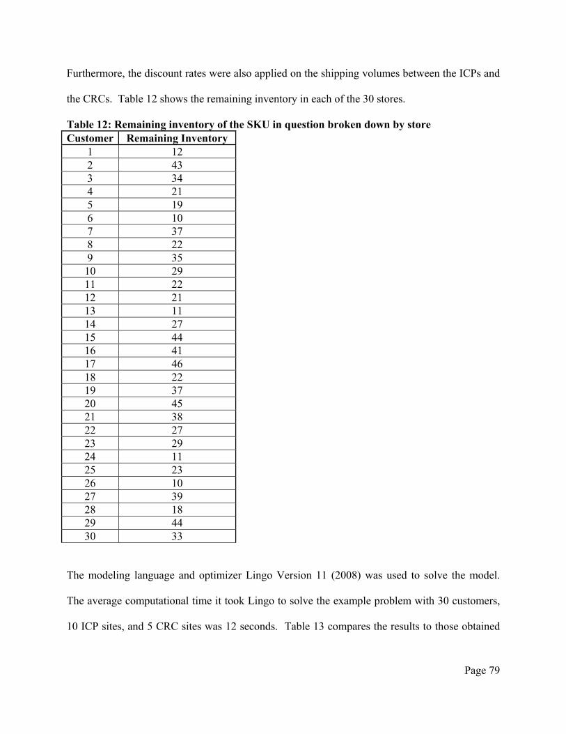
Page 79
Furthermore, the discount rates were also applied on the shipping volumes between the ICPs and
the CRCs. Table 12 shows the remaining inventory in each of the 30 stores.
Table 12: Remaining inventory of the SKU in question broken down by store Customer Remaining Inventory
1 12 2 43 3 34 4 21 5 19 6 10 7 37 8 22 9 35 10 29 11 22 12 21 13 11 14 27 15 44 16 41 17 46 18 22 19 37 20 45 21 38 22 27 23 29 24 11 25 23 26 10 27 39 28 18 29 44 30 33
The modeling language and optimizer Lingo Version 11 (2008) was used to solve the model.
The average computational time it took Lingo to solve the example problem with 30 customers,
10 ICP sites, and 5 CRC sites was 12 seconds. Table 13 compares the results to those obtained

Page 80
by the nonlinear MIP model developed by Min et al. (2006a) along with the results obtained by a
naïve greedy approach using AutoCAD (by assigning each customer to its closest ICP and each
ICP to the closest CRC site). The results show an improvement of almost 10 percent over the
nonlinear MIP model. At the additional $200 cost of opening one more ICP, the MIP model
yielded both inventory and transportation cost savings at the combined amount of $20,745 over
the nonlinear MIP model. This discrepancy can be explained by the fact that the MIP model is
solved for the exact optimal solution, while the nonlinear MIP model was solved by a genetic
algorithm for a local optimum.
Table 13: Cost breakdown and comparison of model results
Costs AutoCAD Nonlinear MIP model MIP model
Total annual cost of renting ICPs $1,800 $800 $1,000
Total cost of establishing CRCs $15,000 $6,000 $6,000
Total inventory costs $31,875 $35,350 $31,875
Total handling costs $21,250 $21,250 $21,250
Total transportation costs $169,200 $148,170 $130,900
Total Annual Reverse Logistics Costs $239,125 $211,570 $191,025
6.4 Sensitivity Analysis
Extensive sensitivity analysis was performed on all levels of the research. Different types
of clustering analysis methods were tested for the various inventory models in order to determine
which one best fit the data. As for the regression analysis, different types of regression for the
different SKUs were run, including but not limited to the simple linear regression. Furthermore,
the normality of the data for each one of the six SKUs was studied to see if there was a
predictable pattern to the mean and standard deviation (See Appendix H). Additionally, the

Page 81
application of preference discount factors to the different prices throughout the phase-out period
was considered in order to realize the effect of marking down prices in a predicted way.
In order to truly test the capability of the proposed linearized model in the reverse
logistics part of the dissertation, showing its capability to solve large-sized problems and to find
a relationship between the optimal collection period T and the parameters of the model, the scope
of the work was broadened by increasing the geographical service area to 100 by 100 miles. The
model was then tested on three problem sizes with 50, 100 and 150 customers. For each
customer size, 10 replications were run, where the geographical locations of the customers,
initial collection points and centralized return centers were randomly generated every time. The
daily return rates for the customers were randomly generated within the range [0, 20]. The
number of ICPs and CRCs remained unchanged at 10 and 5, respectively.
As the number of customers was increased, it resulted in the increase of both the daily
return rate and the volume of products returned from the ICPs to the CRCs, benefitting from the
full effect of the economies of scale from the beginning. On the other hand, computational
results showed that the optimal collection period is increasing as the daily return rate range
decreases and/or the breakpoints for shipping discounts increase (P1 and P2).
Starting with 50 customers, the results showed that in one of the replications, the optimal
collection period T obtained was 4 days, in 8 T was 3 days, and in 1 T was 2 days. Next, keeping
all data the same, another 50 randomly generated customers were added and the model was run
again for 10 replications. The above experiment was repeated by adding 50 more customers.
The results showed that by increasing the number of customers from 50, to 100, and then to 150,
the optimal collection period stays or moves to a lower value in a similar way (see columns of
Table 14).

Page 82
Table 14: Behavior of T as the number of customers increases
Number of Customers Optimal Collection Period T (days)
50 4 3 3 3 3 3 3 3 3 2
100 2 2 2 2 2 2 2 2 2 2
150 2 1 1 1 1 1 1 1 1 1
To illustrate both discrete and continuous analyses, an example was constructed using
parameter values from Table 10. The model was then run with a cluster of customers that had a
total daily return volume of R = 75. All customers returned the products to a single ICP and
subsequently the products were collected during a period T before they were shipped to a single
CRC. Figure 16 displays the total reverse logistics cost for both discrete and continuous values
of T. For the discrete case, the cost function points are depicted as square bullets for integer
values of T = 1…, 10. The function increases at constant rate, while it takes a dip at points
R
Pl .
The critical values of T were found to be 40LR and 86UR using equations (5.4) and (5.5),
respectively. Since UL RRR 75 , the optimal collection period occurs at one of the
intermediates
R
Pl , specifically in this case at T = 6 (confirmed by Theorem 1 and Corollary 1).
If the same data is used, but the continuous case of T is considered, the continuous line segments
have the same slope as the rate of increase in the discrete case. Herein, the exact breaking points
can be located and then highlighted with a vertical line that connects a dip in the total cost.
Where the breakpoints are exactly going to occur can also be indicated. If all the breakpoints are
examined, T = 1, T = R
P1 = 2.67, T = R
P2 = 5.33, and T = R
P3 = 8, the optimal solution occurs at

one of th
This is al
The spec
thereafter
clusters w
capacity
negligibl
compared
periods.
extended
return rat
he intermedi
lso confirme
F
cial structure
r products a
where each
is enforced
le. This spe
d to the shi
In addition
d to consider
tes.
iate breakpo
ed by the con
Figure 16: O
e was based
are transship
cluster is w
d on the CR
ecial structur
ipping break
to the aforem
r the random
oints, since R
ntinuous cas
Optimal peri
on multiple
pped to mul
within the g
RCs, while
re was also
kpoints duri
mentioned c
m, unpredicta
R falls betw
e theorem.
iods in discr
e customers
ltiple CRCs;
geographical
fixed costs
based on a
ng both the
contributions
able nature o
ween LR and
rete vs. cont
returning pr
; however, c
l area of a s
at the ICP
given avera
e discrete an
s of the prop
of customer
d UR , name
tinuous T
roducts to m
customers w
single ICP.
s and CRC
age daily ret
nd the conti
posed model
demands an
Pag
ely T = 5.33
multiple ICP
were divided
In addition
s are consid
turn rate and
inuous colle
, it can be fu
nd the subseq
ge 83
3 + ε.
s and
d into
n, no
dered
d was
ection
urther
quent

Page 84
Chapter 7
Summary and Recommendations for Future
Research
In this final chapter of the dissertation, a summary of the problems solved, models
developed, and their contributions will be presented, as well as a section recommending future
research.
The issues addressed throughout the dissertation dealt with two major aspects of logistics,
inventory and reverse logistics.
Using sales records from a retail chain, a model was developed that can determine the
best prices to set during a phase-out time horizon so that the total initial inventory is depleted and
revenue is maximized. Cluster analysis approach was applied to the data, and then a nonlinear
power regression model was used to determine the best-fit regression equation, based on the
price elasticity of demand. Furthermore, the different SKUs were compared to one another in
order to study the pattern of behavior. The case of the initial inventory being greater than the
total units sold at the end of the phase-out period was also addressed to handle the remaining
inventory. In addition, the problem was looked at from a different perspective, where the
discounted prices were pre-determined, and the question to be answered was related to what

Page 85
stage in the phase-out period should a particular discount be applied and are all the different
values of discounts used?
The second focus was on the products returned at the end of the phase-out period. A
model was used to address the issues of reverse logistics. The main contributions from that
model are: (1) the linearization of the model which eased computational complexity and thus
enabled the identification of the optimal solution for larger customer bases; (2) the handling of
the problem with a broader geographical service area and varying shipping volumes between the
ICP and the CRC, and the prediction of where and when the optimal solution is going to occur;
(3) the determination of a functional relationship between the daily return rate and the optimal
collection period; (4) the analysis as to when the optimal solution will be found by examining
closed form solutions obtained from special structures designed for both discrete and continuous
collection period T.
7.1 Recommendations for Future Research
The following topics can be considered for further research: (1) demand dependency of
SKUs on each other using bundled constraints, (2) customers’ reactions to fluctuation in prices,
(3) the case of stochastic demand, and (4) whether we can apply our models to different types of
relationships between price and demand. Furthermore, the model to determine the best prices
for each time period in the case of remaining inventory will be extended, given a salvage price.
Another future research aspect will be to look into the integer case of the markdown strategy
prices.

Page 86
With regards to an action plan to be presented to pharmacy X and manufacturer Y, the
reports show that there was around $10 million in surplus inventory. Pharmacy X owns
whatever remaining inventory after the phase-out period. The distributor, P&G, does not have
any system in place to purchase back their products, since they are targeted as markdown / sell
through; so the assumption is that they are considered and there is no reverse return / storage
policy. However, P&G will be graded on GMROI which has an inventory component.
Therefore, the following topics could be addressed as recommendations as well as potential
future work:
Minimum fixture presentation and the promotional items that add to the inventory. Thus,
one aspect of the problem is to develop and execute a better planogram.
The replenishment is by SKU and by Store. If one gets sold, it’s registered in the system,
and then one is ordered. The policy depends on demand for replenishment; but does not
depend on demand for the promotional items. There is a different Target Inventory Level
for different stores, which is based on the fixture minimum requirements.
Disorganization disconnect, promotional disconnect.
“Net Requirement System” (i.e.: Tide - if it’s forecasted that one hundred items will be
sold and the store has eighty items, only twenty items will be ordered).
Better forecasting based on previous demand and sales data.
Consequently for the reverse logistics model, future research will be focused on
expanding the geographical area, which will increase the number of customers, the number of
initial collection points, and the number of the centralized return centers. This expansion will
also lead to the increase of the remaining inventory to be handled and transported. Furthermore,

Page 87
a closer look will be given to the economies of scale policies in order to observe the effects of
implementing different approaches.

Page 88
Appendix A: Reverse Logistics Lingo Model
MODEL:
! This is a Mixed Integer Linear Programming Model to deal with the Reverse Logistics Network
for Product Returns;
SETS:
CUSTOMER/1 .. 75/: ri; ICP/1 .. 10/: a, h, Z; CRC/1 .. 5/: ck, m, G; CUSTOMER_ICP(CUSTOMER,ICP): dc_icp, Y; ICP_CRC(ICP,CRC): dicp_crc, X, U1, U2, U3, W1, W2, rjk1, rjk2, rjk3;
ENDSETS
[OBJFUN] MIN = ICP_RENT_COST + CRC_EST_COST + INV_COST + HAND_COST + TRANS_COST; ICP_RENT_COST = @SUM (ICP: a*Z); CRC_EST_COST = @SUM(CRC: ck*G); INV_COST = b*w*((T+1)/2)* @SUM(CUSTOMER: ri); HAND_COST = w*@SUM(CUSTOMER_ICP(i,j)|dc_icp(i,j) #LE# l:ri(i)*h(j)*Y(i,j)); TRANS_COST = (w/T)* @SUM(ICP_CRC:rjk1*U1 + rjk2*U2 -(rjk1-rjk2)*p1*W1+ rjk3*U3 -(rjk2-rjk3)*p2*W2); @FOR(ICP_CRC: [X_U1_U2_U3] X=U1+U2+U3; [U3_W2] U3<= M1*W2; [W2_U2] (p2-p1)*W2 <= U2; [U2_W1] U2 <= (p2-p1)*W1; [W1_U1] p1*W1 <= U1; [U1_1] U1 <= p1;); @FOR(CUSTOMER(i):[CUS_ASSIGN]@SUM(ICP(j)|dc_icp(i,j) #LE# l:Y(i,j)) = 1); @FOR(ICP(j):[OPEN_ICP]@SUM(CUSTOMER(i)|dc_icp(i,j) #LE# l:Y(i,j)) <= M1*Z(j)); @FOR(ICP(j):[FLOW_BALANCE] T*@SUM(CUSTOMER(i)|dc_icp(i,j) #LE#
l:ri(i)*Y(i,j)) = @SUM(CRC(k):X(j,k))); @FOR(CRC(k):@SUM(ICP(j):X(j,k)) <= T*m(k)*G(k)); @FOR(ICP_CRC: [BIN_W1]@BIN(W1); [BIN_W2]@BIN(W2)); @FOR(CUSTOMER_ICP(i,j)|dc_icp(i,j) #LE# l:[BIN_Y]@BIN(Y(i,j))); @FOR(ICP:[BIN_Z]@BIN(Z)); @FOR(CRC:[BIN_G]@BIN(G));

Page 89
DATA:
! Indices; i = 30 index for customers; j = 10 index for initial collection points; k = 5 index for centralized return centers; !Model Parameters; b = 0.1; w = 250; T = 7; a = @OLE(E:\Data.xls); ri = @OLE(E:\Data.xls); rjk1= @OLE(E:\Data.xls); rjk2= @OLE(E:\Data.xls); rjk3= @OLE(E:\Data.xls); h = @OLE(E:\Data.xls); ck = @OLE(E:\Data.xls); m = @OLE(E:\Data.xls); dc_icp = @OLE(E:\Data.xls); dicp_crc = @OLE(E:\Data.xls); l = 25; M1 = 1000; E = 1; alpha1 = 0.8; alpha2 = 0.6; p1 = 200; p2 = 400; beta1 = 1.1; beta2 = 1.2; q1 = 25; q2 = 60;
ENDDATA
END

Page 90
Appendix B: Cluster Algorithm Lingo Model
MODEL: ! This is a Linear Programming Model that deals with the Clustering Algorithm; SETS:
UP/1 .. 54/:P; CM/1 .. 9/:X; UP_CM(UP,CM):Y, Z;
ENDSETS [OBJFUN] MIN = @SUM (UP_CM(i,j): Z(i,j)); @FOR(UP_CM(i,j):M*(1-Y(i,j)) -(P(i)-X(j)) + Z(i,j) >= 0); @FOR(UP_CM(i,j):M*(1-Y(i,j)) -(-P(i)+X(j)) + Z(i,j) >= 0); @FOR(UP(i):@SUM(UP_CM(i,j):Y(i,j)) = 1); @FOR(UP_CM:[BIN_Y]@BIN(Y)); @FOR(CM(j):X(j) <= @MAX(UP(i):P(i))); @FOR(CM(j):X(j) >= @MIN(UP(i):P(i))); DATA: !Model Parameters; P = @OLE(C:\Data.xls); @OLE(C:\Data.xls) = X; M = 100; ENDDATA END

Page 91
Appendix C: Price Elasticity Lingo Model
MODEL: ! This is a Non-Linear Programming Model to deal with the Price Elasticity of Demand; [OBJFUN] MAX = alpha*(P_1^(beta+1)+ P_2^(beta+1)+ P_3^(beta+1) + P_4^(beta+1)+ P_5^(beta+1)+ P_6^(beta+1)+ P_7^(beta+1) + P_8^(beta+1)+ P_9^(beta+1)) + (S_C*R_1); alpha*(P_1^(beta)+ P_2^(beta)+ P_3^(beta) + P_4^(beta)+ P_5^(beta)+ P_6^(beta)+ P_7^(beta) + P_8^(beta)+ P_9^(beta)) + R_1 = vol_tb_depl; DATA: alpha = 37625; beta = -1.605; vol_tb_depl = 20742; S_C = 3.0; @OLE(C:\Documents and Settings\Daisy\Desktop\4.xls) = P_1; @OLE(C:\Documents and Settings\Daisy\Desktop\4.xls) = P_2; @OLE(C:\Documents and Settings\Daisy\Desktop\4.xls) = P_3; @OLE(C:\Documents and Settings\Daisy\Desktop\4.xls) = P_4; @OLE(C:\Documents and Settings\Daisy\Desktop\4.xls) = P_5; @OLE(C:\Documents and Settings\Daisy\Desktop\4.xls) = P_6; @OLE(C:\Documents and Settings\Daisy\Desktop\4.xls) = P_7; @OLE(C:\Documents and Settings\Daisy\Desktop\4.xls) = P_8; @OLE(C:\Documents and Settings\Daisy\Desktop\4.xls) = P_9; @OLE(C:\Documents and Settings\Daisy\Desktop\4.xls) = R_1; ENDDATA END

Page 92
Appendix D: Initial Data Set for the Reverse
Logistics Model
Potential Sites for Initial Collection Points Site Coordinate x y
icp1 29.79 9.00 icp2 53.30 30.96 icp3 58.21 22.61 icp4 52.93 50.01 icp5 54.90 14.92 icp6 9.49 44.46 icp7 38.92 38.55 icp8 42.53 35.52 icp9 23.61 30.13
icp10 26.36 55.96
Potential Sites for Centralized Return Centers Site Coordinate x y
crc1 18.62 15.70 crc2 56.50 26.14 crc3 17.27 10.00 crc4 38.70 20.52 crc5 0.87 56.15
Locations and Daily Demands of Customers Coordinates x y
1 34.13 41.77 2 51.69 56.33 3 10.79 31.54 4 3.50 25.25 5 14.47 31.31 6 9.84 37.85 7 13.72 37.42 8 42.82 44.66 9 28.61 12.91 10 39.86 20.79

Page 93
11 32.75 22.64 12 17.53 51.30 13 25.82 20.26 14 5.99 34.49 15 8.80 37.71 16 35.92 52.13 17 10.72 16.35 18 2.09 47.20 19 23.21 43.28 20 43.39 12.44 21 9.10 13.48 22 10.38 54.81 23 50.97 59.94 24 52.46 59.03 25 56.32 27.23 26 48.61 56.77 27 17.88 55.26 28 56.33 1.24 29 30.74 14.99 30 24.09 34.81

# fr# # TreTesTTTCTL
A
of collectionrequency of establishof establish
Total annual enting ICP
Total cost of stablishing C
Total inventoTotal handlinTotal TranspoCosts Total Annual Logistics Cos
Appen
n
hed CRC hed ICP cost of
CRC ory costs ng costs ortation
Reverse sts
dix E:
Reve
T = 1
1 5
$1,000
$3,000 $21,250 $21,250
$154,400
$200,900
: Solu
erse Lo
Soluti
T = 2
2 4
$800
$6,000 $31,875 $21,250
$129,300
$189,225
tion S
ogistic
ion Summar
T = 3
1 4
$800
$3,000 $42,500 $21,250
$129,510
$197,060
Summa
cs Mo
ry
T = 4
1 4
$800
$3,000 $53,125 $21,250
$129,000
$207,175
ary fo
del
T = 5
1 5
$1,000
$3,000 $63,750 $21,250
$128,820
$217,820
Pag
or the
T = 6
1 5
$1,000
$3,000 $74,375 $21,250
$128,820
$228,445
ge 94
T = 7
1 6
$1,200
$3,000 $85,000 $21,250
$128,820
$239,270
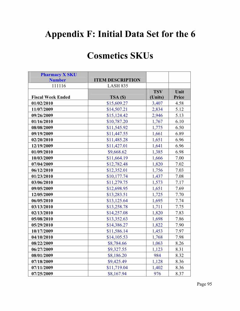
Page 95
Appendix F: Initial Data Set for the 6
Cosmetics SKUs
Pharmacy X SKU Number ITEM DESCRIPTION 111116 LASH 835
Fiscal Week Ended TSA ($) TSV
(Units) Unit
Price 01/02/2010 $15,609.27 3,407 4.58 11/07/2009 $14,507.21 2,834 5.12 09/26/2009 $15,124.42 2,946 5.13 01/16/2010 $10,787.20 1,767 6.10 08/08/2009 $11,545.92 1,775 6.50 09/19/2009 $11,447.55 1,661 6.89 02/20/2010 $11,485.28 1,651 6.96 12/19/2009 $11,427.01 1,641 6.96 01/09/2010 $9,668.62 1,385 6.98 10/03/2009 $11,664.19 1,666 7.00 07/04/2009 $12,782.48 1,820 7.02 06/12/2010 $12,352.01 1,756 7.03 01/23/2010 $10,177.74 1,437 7.08 03/06/2010 $11,279.75 1,573 7.17 09/05/2009 $12,698.95 1,651 7.69 12/05/2009 $13,283.51 1,725 7.70 06/05/2010 $13,125.64 1,695 7.74 03/13/2010 $13,258.78 1,711 7.75 02/13/2010 $14,257.08 1,820 7.83 05/08/2010 $13,352.63 1,698 7.86 05/29/2010 $14,386.27 1,822 7.90 10/17/2009 $11,586.14 1,453 7.97 04/10/2010 $14,105.53 1,768 7.98 08/22/2009 $8,784.66 1,063 8.26 06/27/2009 $9,327.55 1,123 8.31 08/01/2009 $8,186.20 984 8.32 07/18/2009 $9,425.49 1,128 8.36 07/11/2009 $11,719.04 1,402 8.36 07/25/2009 $8,167.94 976 8.37

Page 96
08/15/2009 $9,557.99 1,142 8.37 06/20/2009 $9,790.75 1,168 8.38 10/31/2009 $9,166.70 1,087 8.43 12/26/2009 $11,476.56 1,345 8.53 09/12/2009 $8,588.42 996 8.62 12/12/2009 $10,921.12 1,251 8.73 08/29/2009 $9,030.98 1,034 8.73 02/27/2010 $9,301.58 1,062 8.76 04/24/2010 $11,033.70 1,255 8.79 10/10/2009 $11,723.85 1,329 8.82 11/28/2009 $8,490.97 955 8.89 05/01/2010 $9,997.68 1,122 8.91 02/06/2010 $13,914.88 1,561 8.91 06/26/2010 $9,520.64 1,068 8.91 05/22/2010 $9,985.00 1,120 8.92 04/03/2010 $12,817.10 1,435 8.93 04/17/2010 $10,481.79 1,171 8.95 11/14/2009 $8,837.76 987 8.95 06/19/2010 $10,692.59 1,194 8.96 05/15/2010 $10,379.26 1,158 8.96 03/27/2010 $9,344.07 1,042 8.97 10/24/2009 $9,885.99 1,102 8.97 01/30/2010 $8,561.41 953 8.98 03/20/2010 $10,028.49 1,115 8.99 11/21/2009 $8,986.48 999 9.00 Grand Total $598,039.82 77,989

Page 97
Pharmacy X SKU Number ITEM DESCRIPTION 111115 LASH 830
Fiscal Week Ended TSA ($) TSV
(Units) Unit
Price 01/02/2010 $23,553.62 5,127 4.59 11/07/2009 $19,936.94 3,905 5.11 09/26/2009 $19,159.87 3,745 5.12 01/16/2010 $17,029.94 2,784 6.12 08/08/2009 $14,014.11 2,124 6.60 09/19/2009 $15,044.57 2,174 6.92 01/09/2010 $13,222.29 1,886 7.01 02/20/2010 $15,096.77 2,148 7.03 10/03/2009 $15,302.72 2,170 7.05 06/12/2010 $17,390.09 2,464 7.06 12/19/2009 $14,981.02 2,121 7.06 07/04/2009 $17,301.16 2,448 7.07 01/23/2010 $15,475.69 2,185 7.08 03/06/2010 $15,048.53 2,094 7.19 05/08/2010 $18,176.44 2,344 7.75 09/05/2009 $15,899.30 2,048 7.76 12/05/2009 $18,098.87 2,326 7.78 06/05/2010 $19,227.26 2,466 7.80 03/13/2010 $19,799.86 2,538 7.80 05/29/2010 $19,941.22 2,549 7.82 02/13/2010 $21,785.58 2,769 7.87 04/10/2010 $19,634.06 2,486 7.90 10/17/2009 $16,364.99 2,057 7.96 08/22/2009 $10,693.74 1,289 8.30 08/15/2009 $12,361.76 1,490 8.30 08/01/2009 $9,796.92 1,179 8.31 06/27/2009 $12,666.24 1,524 8.31 06/20/2009 $13,476.01 1,617 8.33 07/25/2009 $11,005.93 1,320 8.34 07/11/2009 $16,019.80 1,920 8.34 07/18/2009 $11,788.64 1,410 8.36 10/31/2009 $12,431.82 1,474 8.43 12/26/2009 $15,703.95 1,840 8.53 09/12/2009 $10,540.29 1,224 8.61 12/12/2009 $14,172.34 1,621 8.74 08/29/2009 $10,014.89 1,140 8.78

Page 98
02/27/2010 $12,995.10 1,479 8.79 10/10/2009 $14,357.35 1,634 8.79 04/24/2010 $14,138.98 1,604 8.81 06/26/2010 $13,657.12 1,536 8.89 05/01/2010 $12,780.13 1,437 8.89 04/03/2010 $16,381.40 1,840 8.90 11/28/2009 $10,990.18 1,234 8.91 05/22/2010 $14,746.58 1,653 8.92 11/14/2009 $11,706.51 1,311 8.93 02/06/2010 $20,331.77 2,274 8.94 05/15/2010 $14,174.59 1,581 8.97 01/30/2010 $12,823.28 1,430 8.97 03/20/2010 $12,397.06 1,381 8.98 06/19/2010 $14,982.50 1,669 8.98 04/17/2010 $13,798.72 1,537 8.98 03/27/2010 $13,317.15 1,483 8.98 10/24/2009 $12,861.54 1,431 8.99 11/21/2009 $12,529.01 1,392 9.00 Grand Total $811,126.20 105,912

Page 99
Pharmacy X SKU Number ITEM DESCRIPTION 111111 LIP 555
Fiscal Week Ended TSA ($) TSV
(Units) Unit
Price 05/15/2010 $3,077.96 985 3.12 07/18/2009 $1,489.20 361 4.13 11/28/2009 $1,206.08 283 4.26 05/08/2010 $2,107.45 456 4.62 03/13/2010 $1,889.09 408 4.63 12/05/2009 $1,389.50 297 4.68 06/05/2010 $1,797.82 377 4.77 07/04/2009 $1,339.77 278 4.82 02/13/2010 $1,708.31 354 4.83 08/08/2009 $1,434.70 295 4.86 10/17/2009 $1,243.47 253 4.91 01/02/2010 $1,035.55 210 4.93 09/26/2009 $1,374.91 274 5.02 10/03/2009 $952.61 164 5.81 08/22/2009 $995.25 171 5.82 04/24/2010 $1,409.81 242 5.83 12/19/2009 $1,171.45 201 5.83 02/20/2010 $1,474.84 253 5.83 06/26/2010 $1,361.66 233 5.84 02/06/2010 $963.46 164 5.87 05/01/2010 $1,272.00 216 5.89 08/29/2009 $1,042.36 177 5.89 07/11/2009 $1,319.80 224 5.89 06/27/2009 $997.61 169 5.90 08/01/2009 $1,098.92 186 5.91 05/29/2010 $1,400.34 237 5.91 09/19/2009 $1,004.63 170 5.91 09/05/2009 $975.19 165 5.91 01/16/2010 $1,111.34 188 5.91 03/06/2010 $1,040.74 176 5.91 05/22/2010 $1,516.07 256 5.92 01/30/2010 $1,078.90 182 5.93 12/12/2009 $889.29 150 5.93 12/26/2009 $1,045.04 176 5.94 04/17/2010 $1,533.23 258 5.94 01/09/2010 $933.05 157 5.94

Page 100
08/15/2009 $1,106.36 186 5.95 06/12/2010 $1,910.25 321 5.95 04/10/2010 $1,322.79 222 5.96 01/23/2010 $1,002.52 168 5.97 10/10/2009 $990.84 166 5.97 03/20/2010 $1,158.66 194 5.97 09/12/2009 $956.30 160 5.98 10/31/2009 $1,274.47 213 5.98 11/07/2009 $1,107.25 185 5.99 02/27/2010 $1,083.49 181 5.99 11/14/2009 $921.96 154 5.99 10/24/2009 $1,143.49 191 5.99 11/21/2009 $964.09 161 5.99 06/20/2009 $1,054.44 176 5.99 03/27/2010 $1,480.53 247 5.99 06/19/2010 $1,367.82 228 6.00 04/03/2010 $1,428.42 238 6.00 07/25/2009 $988.94 164 6.03 Grand Total $68,944.02 12,901

Page 101
Pharmacy X SKU Number ITEM DESCRIPTION 111112 LIP 560
Fiscal Week Ended TSA ($) TSV
(Units) Unit
Price 05/15/2010 $2,632.62 867 3.04 11/28/2009 $951.21 220 4.32 07/18/2009 $1,394.57 320 4.36 07/04/2009 $1,100.40 232 4.74 05/08/2010 $1,669.84 352 4.74 12/05/2009 $1,336.95 280 4.77 06/05/2010 $1,547.22 324 4.78 02/13/2010 $1,200.55 251 4.78 03/13/2010 $1,450.57 298 4.87 08/08/2009 $1,302.51 264 4.93 01/02/2010 $953.78 192 4.97 09/26/2009 $1,175.20 233 5.04 10/17/2009 $1,051.42 208 5.05 02/20/2010 $1,096.89 195 5.63 10/03/2009 $956.28 168 5.69 12/19/2009 $1,037.32 181 5.73 08/22/2009 $781.69 136 5.75 04/24/2010 $993.22 172 5.77 05/01/2010 $1,044.44 180 5.80 09/19/2009 $731.07 125 5.85 07/25/2009 $801.65 137 5.85 01/16/2010 $780.20 133 5.87 11/07/2009 $815.91 139 5.87 08/15/2009 $1,095.87 186 5.89 06/12/2010 $1,522.60 258 5.90 10/10/2009 $814.51 138 5.90 12/26/2009 $838.18 142 5.90 08/01/2009 $891.99 151 5.91 10/24/2009 $851.56 144 5.91 02/06/2010 $727.57 123 5.92 05/29/2010 $996.22 168 5.93 06/26/2010 $960.88 162 5.93 01/23/2010 $635.03 107 5.93 06/20/2009 $973.37 164 5.94 03/06/2010 $837.59 141 5.94 11/21/2009 $827.31 139 5.95

Page 102
07/11/2009 $1,113.65 187 5.96 02/27/2010 $833.80 140 5.96 09/12/2009 $709.31 119 5.96 06/19/2010 $1,102.76 185 5.96 08/29/2009 $780.89 131 5.96 05/22/2010 $1,169.45 196 5.97 04/10/2010 $1,074.11 180 5.97 09/05/2009 $739.96 124 5.97 06/27/2009 $812.04 136 5.97 01/09/2010 $765.02 128 5.98 11/14/2009 $765.42 128 5.98 04/17/2010 $999.63 167 5.99 04/03/2010 $957.80 160 5.99 01/30/2010 $754.54 126 5.99 10/31/2009 $1,199.80 200 6.00 03/20/2010 $1,002.13 167 6.00 03/27/2010 $1,086.00 180 6.03 12/12/2009 $779.61 129 6.04 Grand Total $55,424.11 10,413

Page 103
Pharmacy X SKU Number ITEM DESCRIPTION 111113 LIP 587
Fiscal Week Ended TSA ($) TSV
(Units) Unit
Price 05/15/2010 $3,223.91 988 3.26 07/18/2009 $1,272.48 327 3.89 11/28/2009 $1,117.23 282 3.96 05/08/2010 $1,971.91 429 4.60 03/13/2010 $1,725.76 373 4.63 12/05/2009 $1,699.49 363 4.68 02/13/2010 $1,692.38 358 4.73 08/08/2009 $1,307.54 273 4.79 06/05/2010 $1,657.19 341 4.86 01/02/2010 $1,221.64 251 4.87 07/04/2009 $1,207.92 248 4.87 10/17/2009 $1,450.29 292 4.97 09/26/2009 $2,055.62 409 5.03 10/03/2009 $1,191.22 211 5.65 02/20/2010 $1,060.77 187 5.67 08/01/2009 $906.57 158 5.74 06/26/2010 $878.17 153 5.74 05/29/2010 $1,161.71 202 5.75 08/22/2009 $721.06 125 5.77 12/19/2009 $1,561.26 270 5.78 05/22/2010 $1,125.73 194 5.80 03/06/2010 $1,178.88 203 5.81 06/27/2009 $630.13 108 5.83 08/29/2009 $940.92 161 5.84 09/19/2009 $872.79 149 5.86 07/11/2009 $1,240.03 211 5.88 01/30/2010 $607.09 103 5.89 08/15/2009 $1,031.57 175 5.89 01/09/2010 $737.11 125 5.90 09/12/2009 $772.79 131 5.90 09/05/2009 $957.59 162 5.91 06/20/2009 $786.79 133 5.92 03/27/2010 $1,113.22 188 5.92 04/24/2010 $918.35 155 5.92 12/26/2009 $1,134.49 191 5.94 04/17/2010 $1,035.36 174 5.95

Page 104
03/20/2010 $898.70 151 5.95 05/01/2010 $999.92 168 5.95 06/12/2010 $1,613.29 271 5.95 06/19/2010 $1,042.41 175 5.96 02/06/2010 $739.26 124 5.96 10/24/2009 $1,103.84 185 5.97 10/10/2009 $1,026.48 172 5.97 11/21/2009 $1,051.34 176 5.97 11/14/2009 $973.77 163 5.97 01/23/2010 $682.36 114 5.99 04/10/2010 $1,047.55 175 5.99 01/16/2010 $933.94 156 5.99 04/03/2010 $1,071.71 179 5.99 11/07/2009 $1,083.99 181 5.99 12/12/2009 $1,138.40 190 5.99 07/25/2009 $815.23 136 5.99 10/31/2009 $1,843.53 307 6.00 02/27/2010 $939.74 156 6.02 Grand Total $63,172.42 11,982
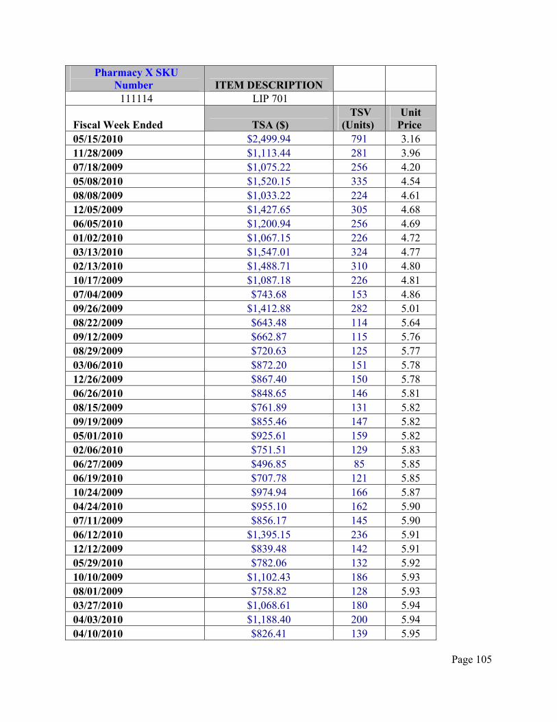
Page 105
Pharmacy X SKU Number ITEM DESCRIPTION 111114 LIP 701
Fiscal Week Ended TSA ($) TSV
(Units) Unit
Price 05/15/2010 $2,499.94 791 3.16 11/28/2009 $1,113.44 281 3.96 07/18/2009 $1,075.22 256 4.20 05/08/2010 $1,520.15 335 4.54 08/08/2009 $1,033.22 224 4.61 12/05/2009 $1,427.65 305 4.68 06/05/2010 $1,200.94 256 4.69 01/02/2010 $1,067.15 226 4.72 03/13/2010 $1,547.01 324 4.77 02/13/2010 $1,488.71 310 4.80 10/17/2009 $1,087.18 226 4.81 07/04/2009 $743.68 153 4.86 09/26/2009 $1,412.88 282 5.01 08/22/2009 $643.48 114 5.64 09/12/2009 $662.87 115 5.76 08/29/2009 $720.63 125 5.77 03/06/2010 $872.20 151 5.78 12/26/2009 $867.40 150 5.78 06/26/2010 $848.65 146 5.81 08/15/2009 $761.89 131 5.82 09/19/2009 $855.46 147 5.82 05/01/2010 $925.61 159 5.82 02/06/2010 $751.51 129 5.83 06/27/2009 $496.85 85 5.85 06/19/2010 $707.78 121 5.85 10/24/2009 $974.94 166 5.87 04/24/2010 $955.10 162 5.90 07/11/2009 $856.17 145 5.90 06/12/2010 $1,395.15 236 5.91 12/12/2009 $839.48 142 5.91 05/29/2010 $782.06 132 5.92 10/10/2009 $1,102.43 186 5.93 08/01/2009 $758.82 128 5.93 03/27/2010 $1,068.61 180 5.94 04/03/2010 $1,188.40 200 5.94 04/10/2010 $826.41 139 5.95

Page 106
05/22/2010 $922.15 155 5.95 01/09/2010 $804.66 135 5.96 12/19/2009 $971.61 163 5.96 10/03/2009 $882.76 148 5.96 02/20/2010 $794.33 133 5.97 04/17/2010 $944.42 158 5.98 09/05/2009 $664.09 111 5.98 10/31/2009 $1,202.69 201 5.98 11/21/2009 $903.69 151 5.98 02/27/2010 $855.87 143 5.99 11/07/2009 $921.76 154 5.99 01/30/2010 $832.11 139 5.99 01/23/2010 $808.25 135 5.99 03/20/2010 $880.15 147 5.99 06/20/2009 $562.96 94 5.99 11/14/2009 $952.36 159 5.99 01/16/2010 $889.12 148 6.01 07/25/2009 $593.41 98 6.06 Grand Total $52,465.46 9,930

Apppenddix G: Reverse Loogisticcs Moc
Page
ck-Up
e 107
p

Page 108
Appendix H: Normality Test for all 6 SKUs
1600150014001300120011001000
Median
Mean
1200115011001050
A nderson-Darling N ormality Test
V ariance 25643.0Skew ness 1.02872Kurtosis 0.72901N 22
M inimum 953.0
A -Squared
1st Q uartile 1025.3M edian 1117.53rd Q uartile 1252.0M aximum 1561.0
95% C onfidence Interv al for M ean
1076.9
0.56
1218.9
95% C onfidence Interv al for M edian
1041.8 1195.6
95% C onfidence Interv al for S tDev
123.2 228.8
P -V alue 0.128
M ean 1147.9S tDev 160.1
9 5 % C onfidence Inter vals
11116 - Summary for (8.50-9.24)
CV = 14%Do not Reject Normality
18001600140012001000
Median
Mean
1700160015001400130012001100
A nderson-Darling Normality Test
V ariance 106079.7Skewness 0.38973Kurtosis -1.68564N 15
Minimum 976.0
A -Squared
1st Q uartile 1087.0Median 1168.03rd Q uartile 1711.0Maximum 1822.0
95% C onfidence Interv al for Mean
1176.0
0.92
1536.7
95% C onfidence Interv al for Median
1100.4 1706.1
95% C onfidence Interv al for StDev
238.5 513.7
P-V alue 0.014
Mean 1356.3StDev 325.7
95% Confidence Intervals
111116 - Summary for (7.75-8.49)
CV = 24%Reject Normality

Page 109
1800170016001500
Median
Mean
17501700165016001550
A nderson-Darling Normality Test
V ariance 13921.4Skewness -0.93036Kurtosis 1.19538N 8
Minimum 1437.0
A -Squared
1st Q uartile 1592.5Median 1680.53rd Q uartile 1748.3Maximum 1820.0
95% C onfidence Interv al for Mean
1566.7
0.26
1764.0
95% C onfidence Interv al for Median
1564.2 1760.1
95% C onfidence Interv al for StDev
78.0 240.1
P-V alue 0.613
Mean 1665.4StDev 118.0
95% Confidence Intervals
111116 - Summary for (7.00-7.74)
CV = 7%Do not Reject Normality
220020001800160014001200
Median
Mean
165016001550150014501400
A nderson-Darling Normality Test
V ariance 60144.5Skewness 1.18182Kurtosis 2.90491N 22
Minimum 1140.0
A -Squared
1st Q uartile 1389.3Median 1509.53rd Q uartile 1638.8Maximum 2274.0
95% C onfidence Interv al for Mean
1424.5
0.49
1642.0
95% C onfidence Interv al for Median
1429.0 1621.4
95% C onfidence Interv al for StDev
188.7 350.5
P-V alue 0.201
Mean 1533.2StDev 245.2
95% Confidence Intervals
111115 - Summary for (8.50-9.24)_1
CV = 16%Do not Reject Normality

Page 110
28002400200016001200
Median
Mean
25002250200017501500
A nderson-Darling Normality Test
V ariance 276060.2Skewness 0.05995Kurtosis -1.60497N 18
Minimum 1179.0
A -Squared
1st Q uartile 1458.0Median 1984.03rd Q uartile 2471.0Maximum 2769.0
95% C onfidence Interv al for Mean
1672.4
0.65
2194.9
95% C onfidence Interv al for Median
1482.3 2402.8
95% C onfidence Interv al for StDev
394.3 787.7
P-V alue 0.073
Mean 1933.7StDev 525.4
95% Confidence Intervals
393495 - Summary for (7.75-8.49)_1
CV = 27%Do not Reject Normality
2500240023002200210020001900
Median
Mean
250024002300220021002000
A nderson-Darling Normality Test
V ariance 35745.7Skewness 0.246040Kurtosis 0.127344N 8
Minimum 1886.0
A -Squared
1st Q uartile 2100.8Median 2159.03rd Q uartile 2382.3Maximum 2464.0
95% C onfidence Interv al for Mean
2031.4
0.48
2347.6
95% C onfidence Interv al for Median
2080.6 2449.0
95% C onfidence Interv al for StDev
125.0 384.8
P-V alue 0.161
Mean 2189.5StDev 189.1
95% Confidence Intervals
111115 - Summary for (7.00-7.74)_1
CV = 9%Do not Reject Normality

Page 111
450400350300250200
Median
Mean
400375350325300275250
A nderson-Darling Normality Test
V ariance 5807.51Skewness 0.489274Kurtosis -0.537319N 10
Minimum 210.00
A -Squared
1st Q uartile 268.75Median 296.003rd Q uartile 384.75Maximum 456.00
95% C onfidence Interv al for Mean
265.68
0.27
374.72
95% C onfidence Interv al for Median
266.81 387.61
95% C onfidence Interv al for StDev
52.42 139.12
P-V alue 0.579
Mean 320.20StDev 76.21
95% Confidence Intervals
111111 - Summary for (4.50 - 5.24)
CV = 24%Do not Reject Normality
320280240200160
Median
Mean
210200190180170
A nderson-Darling Normality Test
V ariance 1440.50Skewness 1.28889Kurtosis 1.66430N 38
Minimum 150.00
A -Squared
1st Q uartile 167.50Median 183.503rd Q uartile 222.50Maximum 321.00
95% C onfidence Interv al for Mean
183.31
1.58
208.26
95% C onfidence Interv al for Median
173.90 196.94
95% C onfidence Interv al for StDev
30.94 49.10
P-V alue < 0.005
Mean 195.79StDev 37.95
95% Confidence Intervals
111111 - Summary for (5.25 - 5.99)
CV = 19%Reject Normality

Page 112
360320280240200
Median
Mean
300280260240220
A nderson-Darling Normality Test
V ariance 2580.71Skewness 0.390983Kurtosis -0.607510N 10
Minimum 192.00
A -Squared
1st Q uartile 226.00Median 257.503rd Q uartile 304.50Maximum 352.00
95% C onfidence Interv al for Mean
227.06
0.15
299.74
95% C onfidence Interv al for Median
223.78 306.90
95% C onfidence Interv al for StDev
34.94 92.74
P-V alue 0.939
Mean 263.40StDev 50.80
95% Confidence Intervals
111112 - Summary for (4.50 - 5.24)_1
CV = 19%Do not Reject Normality
240200160120
Median
Mean
170165160155150145140
A nderson-Darling Normality Test
V ariance 889.00Skewness 1.21876Kurtosis 2.52053N 37
Minimum 107.00
A -Squared
1st Q uartile 132.00Median 142.003rd Q uartile 176.00Maximum 258.00
95% C onfidence Interv al for Mean
144.00
0.95
163.89
95% C onfidence Interv al for Median
137.10 166.70
95% C onfidence Interv al for StDev
24.25 38.73
P-V alue 0.015
Mean 153.95StDev 29.82
95% Confidence Intervals
111112 - Summary for (5.25 - 5.99)_1
CV = 19%Reject Normality

Page 113
400350300250
Median
Mean
400375350325300275250
A nderson-Darling Normality Test
V ariance 4156.23Skewness -0.05086Kurtosis -1.36478N 10
Minimum 248.00
A -Squared
1st Q uartile 267.50Median 349.503rd Q uartile 382.00Maximum 429.00
95% C onfidence Interv al for Mean
287.58
0.30
379.82
95% C onfidence Interv al for Median
265.47 385.32
95% C onfidence Interv al for StDev
44.34 117.69
P-V alue 0.518
Mean 333.70StDev 64.47
95% Confidence Intervals
111113 - Summary for (4.50 - 5.24)_2
CV = 19%Do not Reject Normality
280240200160120
Median
Mean
180175170165160155
A nderson-Darling Normality Test
V ariance 1361.77Skewness 0.71201Kurtosis 1.43348N 39
Minimum 103.00
A -Squared
1st Q uartile 149.00Median 172.003rd Q uartile 188.00Maximum 271.00
95% C onfidence Interv al for Mean
156.88
0.53
180.81
95% C onfidence Interv al for Median
155.94 179.12
95% C onfidence Interv al for StDev
30.16 47.56
P-V alue 0.165
Mean 168.85StDev 36.90
95% Confidence Intervals
111113 - Summary for (5.25 - 5.99)_2
CV = 22%Do not Reject Normality

Page 114
300250200150
Median
Mean
320300280260240220
A nderson-Darling Normality Test
V ariance 3292.77Skewness -0.591564Kurtosis -0.219888N 10
Minimum 153.00
A -Squared
1st Q uartile 225.50Median 269.003rd Q uartile 313.50Maximum 335.00
95% C onfidence Interv al for Mean
223.05
0.33
305.15
95% C onfidence Interv al for Median
225.32 314.79
95% C onfidence Interv al for StDev
39.47 104.76
P-V alue 0.448
Mean 264.10StDev 57.38
95% Confidence Intervals
111114 - Summary for (4.50 - 5.24)_3
CV = 22%Do not Reject Normality
24020016012080
Median
Mean
155150145140135
A nderson-Darling Normality Test
V ariance 807.89Skewness 0.73786Kurtosis 2.02451N 39
Minimum 85.00
A -Squared
1st Q uartile 131.00Median 146.003rd Q uartile 159.00Maximum 236.00
95% C onfidence Interv al for Mean
137.32
0.70
155.75
95% C onfidence Interv al for Median
135.00 151.17
95% C onfidence Interv al for StDev
23.23 36.63
P-V alue 0.061
Mean 146.54StDev 28.42
95% Confidence Intervals
111114 - Summary for (5.25 - 5.99)_3
CV = 19%Do not Reject Normality

Page 115
Index
best fit, 34, 43, 74, 75, 77, 88
bordered Hessian matrix, 46
breakpoints, 55, 59, 66, 68, 69, 72, 89, 90, 91
centralized return centers, 18, 32, 38, 39, 40, 41, 53, 54, 85, 86, 89, 94, 96
centroid, 33
closed form, iii, 19, 20, 32, 41, 60, 61, 69, 83, 93
clustering analysis, 13, 19, 28, 42, 88
collection period, 19, 31, 32, 40, 41, 54, 55, 66, 68, 69, 70, 71, 72, 73, 74, 89, 90, 93
continuous, ii, vii, 19, 25, 58, 59, 61, 72, 73, 90, 91, 93
convex set, 46, 47
determinant, 46
deterministic, 23, 25, 26, 27, 127
dynamic pricing, 21, 22, 53, 124, 125, 128
economies of scale, 38, 55, 69, 72, 73, 89, 94
elastic, vii, 10, 11, 35
elasticity of demand, iii, iv, vii, 9, 13, 18, 21, 28, 34, 35, 43, 77, 80, 92
Euclidean, 29, 30
freight, 31, 39, 40, 54, 55, 66, 72
GMROI, 16, 94, 123
homogeneous, 24
inelastic, vii, 10, 11, 34, 35, 77
initial collection points, 18, 32, 38, 39, 40, 41, 53, 54, 55, 57, 85, 86, 89, 94, 96
Karush-Kuhn-Tucker, 50
K-means, viii, 29, 76
Lagrangean, 44, 45, 46, 48, 51
linear multiple choice knapsack, 64
linearization, iv, 19, 32, 41, 93
Logistics logistics, iii, v, vi, 13, 30, 66, 85, 88, 95,
99, 101, 114, 126, 127
markdown, iii, iv, viii, 12, 13, 16, 18, 19, 26, 27, 41, 74, 79, 81, 82, 83, 85, 93, 94, 124
Markovian, 28, 127
Minkowski metric, 30
mixed integer linear programming, 19
Myopic, 22, 123
Net Requirement System, 15, 94
nonlinear, iii, iv, 13, 31, 32, 34, 40, 45, 50, 52, 87, 92
optimality, 48, 50, 51, 62, 63, 64, 70, 71, 127
original equipment manufacturers, 32, 39
phase-out, iii, iv, viii, 12, 13, 15, 16, 17, 18, 19, 37, 38, 41, 42, 43, 49, 53, 60, 61, 63, 65, 79, 80, 81, 82, 89, 92, 93, 94
Poisson, 24
product returns, iv, viii, 14, 17, 18, 19, 28, 30, 31, 32, 38, 40, 69, 72, 73, 126
regression, 13, 18, 33, 43, 49, 74, 75, 77, 79, 81, 88, 92
reservation price, 21, 22, 24
reverse logistics, iii, viii, 13, 14, 17, 19, 20, 21, 28, 30, 31, 32, 39, 40, 41, 42, 53, 57, 68, 69, 81, 84, 85, 86, 89, 90, 92, 93, 94
salvage, viii, 13, 16, 18, 23, 25, 28, 36, 37, 48, 49, 53, 61, 65, 80, 81, 82, 83, 85, 93
SKU, vii, viii, 16, 36, 37, 45, 75, 76, 77, 78, 79, 80, 81, 82, 83, 87, 94, 102, 104, 106
stochastic, 23, 27, 93, 124, 125
Unit Price, 33, 34, 76, 102, 104, 106, 108, 110, 112, 123
weighted average, 68, 69

Page 116
List of Abbreviated Terms
CRC Centralized Return Center
D / I Dependent vs. Independent
GA Generic Algorithm
GMROI Gross Margin Return on Inventory
ICP Initial Collection Point
KKT Karush – Kuhn – Tucker
LMCK Linear Multiple Choice Knapsack
MIP Mixed Integer Program
M / S Myopic vs. Strategic
OEM Original Equipment Manufacturers
R / NR Replenishment vs. No Replenishment
SKU Stock Keeping Unit
TSA Total Sales Amount
TSV Total Sales Volume
UP Unit Price
WA Weighted Average

Page 117
References
1. Barros, A.I., Dekker, R., and Scholten, V., 1998. A two-level network for recycling sand: A case study. European Journal of Operational Research 110, 199-214.
2. Biller, S., Chan, L.M.A., Simchi-Levi, D., Swann, J.L., 2005. Dynamic pricing and the
direct-to-customer model in the automotive industry. Electronic Commerce Research 309-334.
3. Bitran, G. R., Mondschein, S., 1997. Periodic pricing of seasonal products in retailing. Management Science 43, 64-79.
4. Bitran, G. R., Caldentey, R., Mondschein, S., 1998. Coordinating clearance markdown sales
of seasonal products in retail chains. Operations Research 46 (5), 609–624. 5. Chan, L. M. A., Simchi-Levi, D., Swann, J., 2001. Effective dynamic pricing strategies with
stochastic demand. Massachusetts Institute of Technology, Cambridge, MA. 6. Chan, L.M.A., Muriel A., Shen Z. M., Simchi-Levi D., and Teo C., 2002. Effective zero
inventory ordering policies for the single warehouse multi-retailer problem with piecewise linear cost structures. Management Science 48 (11), 1446-1458.
7. Chen, X., Simchi-levi, D., 2002. Coordinating inventory control and pricing strategies with
random demand and fixed ordering cost. Massachusetts Institute of Technology, Cambridge, MA.
8. Chen, X., Simchi-Levi, D., 2003. A new approach for the stochastic cash balance problem
with fixed costs. Massachusetts Institute of Technology, Cambridge, MA. 9. Chen, X., Simchi-Levi, D., 2004. Coordinating inventory control and pricing strategies with
random demand and fixed ordering cost: The infinite horizon case. Math. Operations Research Forthcoming.
10. Coy, P., 2000. The power of smart pricing. Business Week (April 10). 11. Del Castillo, E., and Cochran, J.K., 1996. Optimal short horizon distribution operations in
reusable container systems. Journal of the Operational Research Society 47(1), 48-60. 12. Eliashberg, J. and Steinberg, R., 1993. Marketing-production joint decision-making.
Operations Research and Management Science, Vol. 5, Elsevier, Amsterdam 827–880. 13. Elmaghraby, W., Keskinocak, P., 2003. Dynamic pricing in the presence of inventory
considerations: research overview, current practices, and future directions. Management Science 49, 1287-1309.

Page 118
14. Federgruen, A., Heching, A., 1999. Combined pricing and inventory control under
uncertainty. Operations Research 47, 454-475.
15. Feng, Y., Chen, F., 2003. Joint pricing and inventory control with setup costs and demand uncertainty. Chinese University of Hong Kong, Hong Kong.
16. Feng, Y., Gallego, G., 1995. Optimal starting times for end-of-season sales and optimal
stopping-times for promotional fares. Management Science 41, 1371-1391. 17. Ferguson, M., Guide, V., Daniel, R., Jr., and Souza, G.C., 2006. Supply chain coordination
for false failure returns. Manufacturing & Service Operations Management 8(4), 376-393.
18. Fleischmann, M., Krikke, H.R., Dekker, R., and Flapper, D.P., 2000. A characterization of logistics networks for product recovery. Omega 28, 653-666.
19. Fleischmann, M., 2003. Reverse logistics network structures and design. In: L.N. Van
Wassenhove and V.D.R. Guide, Jr. (Ed.), Business Aspects of Closed-Loop Supply Chains: Exploring the Issues. The Carnegie Bosch Institute, pp. 117-148.
20. Gallego, G., Van Ryzin, G. J., 1994. Optimal dynamic pricing of inventories with stochastic
demand over finite horizon. Management Science 40, 999-1020. 21. Gecker, R., 2007. Industry best practices in reverse logistics, Unpublished White Paper,
Aberdeen Group.
22. Guide, V.D.R., Jr., Harrison, T.P., and Van Wassenhove, L.K., 2003. The challenges of closed-loop supply chains. Interfaces 33(6), 3-6.
23. Gupta, D., Hill, A., Bouzdine-Chameeva, T., 2004. A pricing model for clearing end-of-
season retail inventory. European Journal of Operational Research 170, 518-540. 24. Jayaraman, V., Guide, Jr., V.D.R., and Srivastava, R., 1999. A closed-loop logistics model
for remanufacturing. Journal of the Operational Research Society 50, 497-508.
25. Jayaraman, V., Patterson, R.A., and Rolland, E., 2003. The design of reverse distribution networks: Models and solution procedures. European Journal of Operational Research 150, 128-149.
26. Kimes, S. E., 1989. A tool for capacity-constrained service firms. Journal of Operations
Management 8(4), 348–363. 27. Kozanidis, G., Melachrinoudis, E., 2002. A mixed integer knapsack model for allocating
funds to highway safety improvements. Transportation Research 36, 789–803.

Page 119
28. Kozanidis, G., Melachrinoudis, E., 2004. A branch & bound algorithm for the 0-1 mixed integer knapsack problem with linear multiple choice constraints. Computers and Operations Research 31, 695–711.
29. Krikke, H.R., Kooi, E.J., and Schurr, P.C., 1999. Network design in reverse logistics: A
quantitative model. In: Stähly, P. (Ed.), new trends in distribution logistics. Springer Verlag, Berlin, 45-62.
30. Lazear, E. P., 1986. Retail pricing and clearance sales. American Economic Review 76, 14-
32. 31. Lin, E.Y.-H., 1998. A bibliographical survey on some well-known non-standard knapsack
problems. INFOR (36), 274-317. 32. Lingo Systems, Inc., 2008. Lingo: The Modeling Language and Optimizer, Chicago, IL. 33. McCullough, K., Dolberg, S., Leyne, L., Reinhard, A.A., Gatoff, J., 1999. Mastering
commerce logistics. Forrester Research Report, Cambridge, MA, August 1999.
34. Melachrinoudis, E., Min, H., and Wu, X., 1995. A multi-objective model for the dynamic location of landfills. Location Science 3(3), 143-166.
35. Meyer H., 1999. Many happy returns. The Journal of Business Strategy, 20(4), 27-31. 36. Min, H., 1989. A bi-criterion reverse distribution model for product recall. Omega, 17(5),
483-490. 37. Min, H., Ko, H.K., and Ko, C.S., 2006a. A genetic algorithm approach to developing the
multi-echelon reverse logistics network for product returns. Omega, 34(1), 56-59.
38. Min, H., Ko, C.S., and Ko, H.K., 2006b. The spatial and temporal consolidation of returned products in a closed-loop supply chain network. Computers and Industrial Engineering, 51(2), 309-320.
39. Norman, L. and Sumner, W., 2006. The sixth hidden costs of reverse logistics. Reverse
Logistics Magazine, www.RLmagazine.com.
40. Petruzzi, N. C., Dada, M., 1999. Pricing and the newsvendor model: A review with extensions. Operations Research 47, 183–194.
41. Polatoglu, H., Sahin, I., 2000. Optimal procurement policies underprice dependent demand.
International Journal Production Economics 65, 141–171.
42. Porteus, E., 1971. On the optimality of the generalized (s, S) policies. Management Sci. 17, 411–426.

Page 120
43. Rajan, A., Rakesh, R. Steinberg., 1992. Dynamic pricing and ordering decisions by a monopolist. Management Science 38, 240-262.
44. ReturnBuy, 2000. The new dynamics of returns: The profit, customer and business
intelligence opportunities in returns. White Paper, Ashburn, Virginia: ReturnBuy.com, December.
45. Scarf, H. 1960. The optimality of (s, S) policies for the dynamic inventory problem. Proc. 1st
Stanford Symposium on Mathematical Methods Social Sciences. Stanford University Press, Stanford, CA.
46. Schultmann, F., Engels, B., and Rentz, O., 2003. Closed-loop supply chains for spent
batteries. Interfaces, 33(6), 57-71. 47. Schultmann, F., Zumkeller, M., and Rentz, O., 2005. Modeling reverse logistic tasks within
closed-loop supply chains: an example from the automotive industry. European Journal of Operational Research, 171(3), 1033-1050.
48. Sethi, P. S., F. Cheng. 1997. Optimality of (s, S) policies in inventory models with
Markovian demand. Operations Research 45(6), 931–939. 49. Shear H., Speh, T.W., and Stock, J.R., 2003. The warehousing link of reverse logistics.
Presented at the 26th Annual Warehousing Education and Research Council Conference, San Francisco, CA.
50. Smith, S., Achabal, D., 1998. Clearance pricing and inventory policies for retail chains.
Management Science 44, 285-300. 51. Srivastava, R., 2007. Network design for reverse logistics. Omega 36(4), 535-548.
52. Stock, J.R., 1992. Reverse logistics, White Paper, Oak Brook, IL: Council of Logistics
Management.
53. Thomas, L., 1970. Price-production decisions with deterministic demand. Management Science 16, 747-750.
54. Thomas, L. J., 1974. Price and production decisions with random demand. Operations
Research 22, 513–518. 55. Whitin, T. M. 1955. Inventory control and price theory. Management Sci. 2, 61–80. 56. Thowsen, G. T., 1975. A dynamic nonstationary inventory problem for a price/quantity
setting firm. Naval research logistics quarterly 22, 461-476.
Page 121
57. Van Wassenhove, L. N., and Guide, V. D. R. Jr., 2003. End of life returns: Closed loop supply chains. In: L. N. Van Wassenhove & V. D. R. Guide, Jr. (Eds.), Business aspects of closed-loop supply chains. The Carnegie Bosch Institute, exploring the issues (pp. 9–14).
58. Zabel, E., 1970. Monopoly and uncertainty. Revenue of Economic Studies 47, 205-219. 59. Zhao, W., Zheng, Y. S., 2000. Optimal dynamic pricing for perishable assets with non-
homogenous demand. Management Science 46(3), 375-388.

Page 122
Additional Book References 1. Bertsekas, D., 1995. Dynamic Programming and Optimal Control, Vol. 1. Athena
Scientific, Belmont, MA.
2. Hillier, F. S., Lieberman, G. J., 2010. Introduction to Operations Research, ninth edition. McGraw-Hill Higher Education.
3. Taha, H., 2006. Operations Research: An Introduction, eighth edition. Prentice Hall, New Jersey.
4. Topkis, D. M., 1998. Supermodularity and Complementarity. Princeton University Press,
Princeton, NJ.